sustainability

Article

Is the High Interest Rate Combined with IntenseDeleveraging Campaign Desirable? A CollateralMechanism under Stringent Credit Constraints

Qiuyi Yang 1, Youze Lang 2,* and Changsheng Xu 1

1 School of Economics, Huazhong University of Science and Technology, 1037 Luoyu Road,Wuhan 430074, China; qiuyi_yang@hust.edu.cn (Q.Y.Y.); chshxu@hust.edu.cn (C.S.X.)

2 School of Economics, Shanghai University of Finance and Economics, 111 Wuchuan Road,Shanghai 200433, China

* Correspondence: falelang@163.sufe.edu.cn; Tel.: +86-185-2106-7192

Received: 17 November 2018; Accepted: 13 December 2018; Published: 16 December 2018 �����������������

Abstract: Recently, China has witnessed a continuously increasing Debt-to-GDP ratio and a vigorouslyexpanding shadow banking sector. Housing prices hovering at a high level seriously affect the livesof ordinary residents. Disappointingly, a variety of activities such as intense deleveraging campaignsand tight monetary controls produce little effect. Why do these seemingly rightful implementationshardly work? What should governments do to stop the incessant expansion of asset bubbles? Whatrole ought financial supervisors to play in regulating credit markets and facilitating a sustainableand inclusive economic growth? This paper sets off from the pledgeability of asset bubbles andconstructs a generalized overlapping generation (OLG) model incorporating financial frictions andcollateral constraints, in order to explore the bubble evolution under the alterations of marketinterest rates and credit conditions. The results show a unique bubble equilibrium, in which thesteady-state bubble size expands when interest rate increases. Numerical results further revealthat the bubble-inflation effect of a higher interest rate is reinforced by a more stringent collateralconstraint. Our research contributes to an explanation of the inefficacy of present policies andprovides the following policy implications: The combination of an interest rate elevation and astrong loan restriction is in fact undesirable for suppressing asset bubbles. Not merely does it strikeproductivity and capital formation, but it also fosters investors to hold more risky assets to solveliquidity shortage under constrained borrowing capacity.

Keywords: sustainable financial market; asset bubbles; overlapping generation (OLG) model; marketinterest rate; credit constraints; pledgeability; financial regulation and supervision

1. Introduction

After the 2008 global financial crisis, both the housing market and the stock market all over theworld showed drastic fluctuations in asset prices, in a general background of an imperfect creditenvironment. Should government strengthen policy control to manage inflated asset bubbles? Cana rise in interest rate hold down bubbles efficiently and can contractionary policy implementationsmitigate any economic downturn? This ostensibly reasonable belief has reached a general consensusin theory and practically guides the interventions and supervisions in financial markets for years.Nevertheless, there have been dozens of counterexamples of a “price puzzle” where stringent interestrate policy pushes up asset prices and inflates bubbles, which has drawn public attention.

At the same time, in China, in face of the soaring housing prices and the over-leveragedfinancial systems of recent years, the Chinese government and the People’s Bank of China have

Sustainability 2018, 10, 4803; doi:10.3390/su10124803 www.mdpi.com/journal/sustainability

Sustainability 2018, 10, 4803 2 of 22

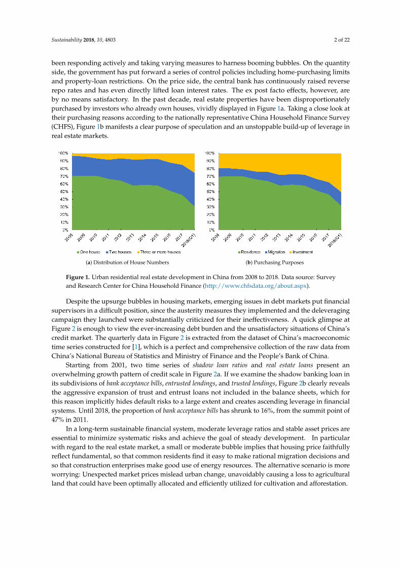
been responding actively and taking varying measures to harness booming bubbles. On the quantityside, the government has put forward a series of control policies including home-purchasing limitsand property-loan restrictions. On the price side, the central bank has continuously raised reverserepo rates and has even directly lifted loan interest rates. The ex post facto effects, however, areby no means satisfactory. In the past decade, real estate properties have been disproportionatelypurchased by investors who already own houses, vividly displayed in Figure 1a. Taking a close look attheir purchasing reasons according to the nationally representative China Household Finance Survey(CHFS), Figure 1b manifests a clear purpose of speculation and an unstoppable build-up of leverage inreal estate markets.

(a) Distribution of House Numbers (b) Purchasing Purposes

Figure 1. Urban residential real estate development in China from 2008 to 2018. Data source: Surveyand Research Center for China Household Finance (http://www.chfsdata.org/about.aspx).

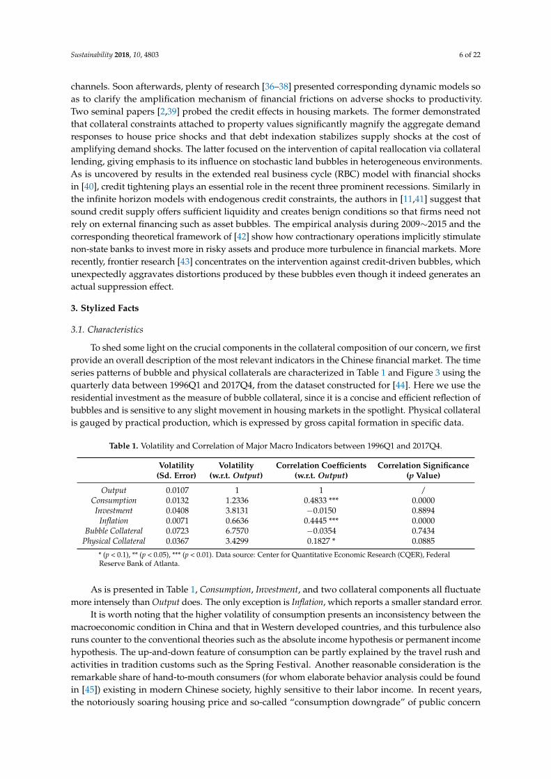
Despite the upsurge bubbles in housing markets, emerging issues in debt markets put financialsupervisors in a difficult position, since the austerity measures they implemented and the deleveragingcampaign they launched were substantially criticized for their ineffectiveness. A quick glimpse atFigure 2 is enough to view the ever-increasing debt burden and the unsatisfactory situations of China’scredit market. The quarterly data in Figure 2 is extracted from the dataset of China’s macroeconomictime series constructed for [1], which is a perfect and comprehensive collection of the raw data fromChina’s National Bureau of Statistics and Ministry of Finance and the People’s Bank of China.

Starting from 2001, two time series of shadow loan ratios and real estate loans present anoverwhelming growth pattern of credit scale in Figure 2a. If we examine the shadow banking loan inits subdivisions of bank acceptance bills, entrusted lendings, and trusted lendings, Figure 2b clearly revealsthe aggressive expansion of trust and entrust loans not included in the balance sheets, which forthis reason implicitly hides default risks to a large extent and creates ascending leverage in financialsystems. Until 2018, the proportion of bank acceptance bills has shrunk to 16%, from the summit point of47% in 2011.

In a long-term sustainable financial system, moderate leverage ratios and stable asset prices areessential to minimize systematic risks and achieve the goal of steady development. In particularwith regard to the real estate market, a small or moderate bubble implies that housing price faithfullyreflect fundamental, so that common residents find it easy to make rational migration decisions andso that construction enterprises make good use of energy resources. The alternative scenario is moreworrying: Unexpected market prices mislead urban change, unavoidably causing a loss to agriculturalland that could have been optimally allocated and efficiently utilized for cultivation and afforestation.

Sustainability 2018, 10, 4803 3 of 22

0

100

200

300

400

500

600

0%

5%

10%

15%

20%

25%

30%

RM

B b

illion

Shadow loan ratio Real estate loan

(a) Credit Growth (b) Decomposition of Shadow Banking Loans

Figure 2. Credit growth and evolution of shadow loan composition in China’s credit market between2001Q4 and 2018Q2 (quarterly). Shadow loan ratio is the “end-of-quarter total lending in the shadowbanking industry” divided by the “end-of-quarter total financial institution loans outstanding”.Real estate loans are “new loans to real estate” deflated by a CPI deflator. Data source: Center forQuantitative Economic Research (CQER), Federal Reserve Bank of Atlanta.

Despite the best of intentions and efforts, as a matter of fact, neither the present strict controlmeasures on real estate nor stringent market regulations on credit are of great advantage to thelong-term sustainability and robust growth in housing markets, at least based on the evidence inChina. Why does the contractionary monetary policy in a harsh credit environment fail to changethese problematic situations? What role should financial supervisors play in regulating asset bubblesin the emergence of sustainable finance? These are all pretty significant issues worth addressing.

The contribution of this paper is summarized as follows. First, most of the scholars who followhousing bubbles with interest concentrate on the U.S. market, as in [2–5], yet unfortunately have notdug into the Chinese economy with enormous potential. In addition, among all the abundant researchdevoted to harness housing bubbles, previous scholars have seldom conducted a systemic study on thecompound effect of a twofold austerity measure, featured by an upward interest rate and a rigid creditrestriction. Our work contributes to the existing literature and adds to the above research gaps byinvestigating thoroughly the unintended consequences of this twofold policy measure and providinga plausible explanation for the unsolved real estate bubbles. Starting from the counter-intuitivephenomenon of the swelling asset bubble and deteriorated debt conditions under tight monetarypolicies and strong deleveraging operations in China’s financial market, this paper attempts to addressthis issue by developing a generalized overlapping generation (OLG) model in a standard NewKeynesian framework, widely applied in the literature on asset markets and monetary policy.

Second, while the literature of monetary effects on asset prices is broad and sufficient, it lacks athorough inquiry into one essential function of bubble assets: mortgage financing. This paper placesparticular emphasis on the pledgeability of rational asset bubbles in investor collateral composition andexplores the effects of changes in market interest rates from the perspective of a collateral mechanismin monetary transmissions. As heated debates pay much attention to the growing risks posed by thebulky share of pledged real estates and accumulated liquidity pressures on borrowers, this work haspractical relevance to the future sustainability and development of the Chinese financial market, whichis closely bound up with the global economy at a higher level from the current situation.

Furthermore, we also make theoretical extensions on a few pioneering studies: We augment [6]by allowing entrepreneurs and general workers to hold bubbles. We also justify the crowd-outeffect of bubbles on capital accumulation in [7,8]. Infinite-horizon models, e.g., [9–11], focus on theeffects on investment and the allocation of stock price bubbles with positive dividends. Our workextends and modifies them by concentrating on the pure bubbles that serve as a store of value traded

Sustainability 2018, 10, 4803 4 of 22

by overlapping agents, aiming at better fitting the reality of housing markets and evaluating thecomprehensive influence in overlapping generations.

The line of reasoning in our logical framework processes is described below: Rational bubblesenter asset markets following [12] and serve as a portion of collaterals used for loan investment ofentrepreneurs (henceforth referred to as “bubble collateral”). These intrinsically valueless assetsproduce no real payoff, expand when market return increases, and further appreciate with pledgeablefeature. Meanwhile, on the production side, the correspondingly rising cost brought by increasedinterest rate hampers capital accumulation and production, depreciating the aggregate value ofordinary pledgeable assets (referred to as “physical collateral”). The composition of bubble andphysical collaterals is utilized by representative investors in our model to satisfy their liquiditydemand. In this situation, when investors bear stringent credit constraints and cannot borrow enoughmoney with the available physical collateral, they will have motivations to add holdings for bubblesto alleviate the liquidity shortage. Additionally, taking the collateral mechanism in credit constraintsinto consideration, an intuitive inference extended here is that the above expansion effect of the risinginterest rate on asset bubbles will be further reinforced if the borrowing restrictions become more rigid.

The rest of this paper is organized as follows: Section 2 summarizes related literature. Section 3displays the stylized facts regarding bubbles and credit in China and empirical evidence with respectto a standard interest rate shock. Section 4 sets up the complete theoretical model considering creditfrictions and bubble asset pledgeability. Section 5 discusses in detail the mathematical and numericalresults, including the steady-state analysis of bubbly equilibrium, the comparative statics of collateralcomposition evolutions and impulse responses under the change in interest rates and the degree ofcredit frictions. Section 6 concludes, puts forward policy implications, and discourses limitations andfuture research. Appendices A and B contain technical proofs.

2. Literature Review

In view of the special nature of a speculative bubble generating no endogenous productivity,it is appropriate to regard it as an inherently valueless premium above price fundamental, within thescope of a pure rational bubble attached to positive price. In real transactions, dealers acknowledgethat bubbles can burst in the unknown future. As is early illustrated in [13], the price of a speculativebubble is driven by the self-fulfilling mechanism of expectation. Bubbles expand as agents haveconfidence in sustained economic growth. With a rising risk premium and a rigid credit condition,continuous bubble inflation finally triggers a sudden collapse in investor sentiment and subsequentlyprovokes a slump in financial markets. To make it worse, when we look into the real estate assetmarket specifically, a housing asset bears expensive transaction costs and confined short selling as atypical class of illiquid asset. As a factual matter, the frenzied overbuilding may be largely ascribed toan endogenous housing supply, well explained in [14]. A more inelastic housing supply breeds bubblesmore easily, extends its duration, and exerts a profound impact on new construction and public welfare.In light of the grave consequences of bubble bursting, whether and how government and supervisorsshould react to asset bubbles have caused much controversy in academic and political circles.

Prior scholars who are in favor of tight policy have focused on the effects of the “reverse operation”on curbing the steep rise of asset prices, appeasing fluctuated financial markets and in this mannerbenefiting macro economic stability. The authors in [15] pointed out the ignorance of future pricevariations in the monetary policy regime of inflation targeting, and claimed that this weakness couldbe overcome by letting interest rates react to asset prices. Based on the theoretical framework of [16],the generation and evolution of bubbles have no influence on the future path of expected inflation,since rational agents perfectly anticipate that bubbles are destined to vanish in the future. Under thiscircumstance, the prevailing inflation targeting is invalid and could only apply “reverse operation”to asset prices so as to cool down the overheated economy. Soon after, the conference report of [17]speaks highly of the superiority of the “leaning against the wind” policy in regulating financialmarkets. Subsequent research in the Bank for International Settlements [18] and empirical evidence in

Sustainability 2018, 10, 4803 5 of 22

Singapore [19] both back up this argument. Using a Bayesian likelihood approach, the supplement roleof prompt policy adjustments to macro prudent policies has been well reflected in the estimated DSGEmodel in [20]. Similarly, the authors in [21] highlight the complementary effect of tight interest rateson banking supervision and regulation. Of recent years, in regard to some dissenting opinions of strictactions and market controls, the authors in [22] stress the far-reaching positive impacts on long-runsustained economic stability at the expense of sacrifice for the moment. Likewise, in a forthcomingtheoretical study, the authors in [23] arrive at the conventional conclusion that a tightening policycontrol is optimal for decreasing bubble fluctuation.

In practice, however, numerous unsuccessful cases arouse suspicion for the actual effect ofausterity campaigns. It is undeniable that a promotion of interest rate raises borrowing costs and harmsmaterial production. When the regulators do not have a clear knowledge of whether the climbing pricesand red-hot economy stem from positive technological advances or bloated financial bubbles, a blindintervention for the purpose of stabilizing financial markets is very likely to generate the oppositeoutcome. The famous discussion in [24,25] conservatively advocates a “benign neglect” strategy whenthe economy confronts multiple shocks. This argument is soon supported and underlined by theauthors in [26], who point out the possible scenario that one action aiming at quelling volatility in acertain market transfers pressure to other markets in the general equilibrium system and in the enddisturbs market order through the feedback loop among market traders. Indeed, improper interferenceand credit squeeze can give rise to bubble collapses and the closely following violent aftermath offinancial turmoil, discussed in detail by the authors in [27]. Fully aware of the great transformationwith the advent of Economic and Monetary Union (EMU), the authors in [28] showed that demographicfactors encourage housing bubbles to expand under relaxed financial constraints in Ireland and Spain.By virtue of the idiosyncrasy in housing markets across the Euro Area, the EMU monetary policy thattargets the region as a whole barely works to control bubbles. For the sake of promoting sustainableeconomic growth associated with a compatible throughput rate not exceeding the carrying capacity ofour finite planet, the authors in [29] call for the necessary restoration of money creation to supportsufficient investment in pivotal public goods, with the cardinal aim of realizing the transition to asteady-state economy based on harmony and well-being. More recently, the authors in [12] account forthe root reason why a rational asset bubble has a growth rate in accord with the market interest rate inpartial equilibrium, and then set up a succinct and elegant general equilibrium model demonstratingthat the design of an optimal monetary policy should judge and weigh the trade-off between bubblestabilization and inflation stabilization, and not only comply with the policy of “leaning against thewind.” Shortly after, this argument was further backed by empirical evidence in [30], which revealsan evolution pattern in the U.S. stock market that prices decrease when the economy is exposed to atightened monetary policy. From the historical dimension looking back on the well known bubbles inthe past 400 years, the authors in [31] summarize previous experiences and suggest that macro prudentmeasures, rather than strong interest rate tools, are more helpful to dampen bubble developments.In a comprehensive cost-and-benefit analysis, the authors in [32] arrive at the clear-cut conclusionthat the marginal cost is much higher than the benefit for reverse operation in response to high assetprices. Apart from that, the authors in [33] indicate that government and supervisors substantiallyunderestimate the extremely high costs produced by financial imbalances and policy misuse. Thus,the implementation of interest rate controls requires utmost caution.

In parallel with contractionary monetary policy, a very commonly used supplementary action iscredit restriction. During the intense process of deveraging compaign, China has proposed rigorousrules regulating the financial industry, including enforcing specific liquidity requirements, shuttingdown peer-to-peer platforms and toughening supervision over micro lending firms. As a vital channelin the monetary transmission mechanism, credit supply is a topic of specific concern in the relatedliterature. First explored in [34], the credit channel damages investment and production by diminishingproductive collateral value and debt capacity. The full and accurate research in [35] elucidates howimperfection in credit markets accelerates monetary effects through the balance sheet and bank lending

Sustainability 2018, 10, 4803 6 of 22

channels. Soon afterwards, plenty of research [36–38] presented corresponding dynamic models soas to clarify the amplification mechanism of financial frictions on adverse shocks to productivity.Two seminal papers [2,39] probed the credit effects in housing markets. The former demonstratedthat collateral constraints attached to property values significantly magnify the aggregate demandresponses to house price shocks and that debt indexation stabilizes supply shocks at the cost ofamplifying demand shocks. The latter focused on the intervention of capital reallocation via collaterallending, giving emphasis to its influence on stochastic land bubbles in heterogeneous environments.As is uncovered by results in the extended real business cycle (RBC) model with financial shocksin [40], credit tightening plays an essential role in the recent three prominent recessions. Similarly inthe infinite horizon models with endogenous credit constraints, the authors in [11,41] suggest thatsound credit supply offers sufficient liquidity and creates benign conditions so that firms need notrely on external financing such as asset bubbles. The empirical analysis during 2009∼2015 and thecorresponding theoretical framework of [42] show how contractionary operations implicitly stimulatenon-state banks to invest more in risky assets and produce more turbulence in financial markets. Morerecently, frontier research [43] concentrates on the intervention against credit-driven bubbles, whichunexpectedly aggravates distortions produced by these bubbles even though it indeed generates anactual suppression effect.

3. Stylized Facts

3.1. Characteristics

To shed some light on the crucial components in the collateral composition of our concern, we firstprovide an overall description of the most relevant indicators in the Chinese financial market. The timeseries patterns of bubble and physical collaterals are characterized in Table 1 and Figure 3 using thequarterly data between 1996Q1 and 2017Q4, from the dataset constructed for [44]. Here we use theresidential investment as the measure of bubble collateral, since it is a concise and efficient reflection ofbubbles and is sensitive to any slight movement in housing markets in the spotlight. Physical collateralis gauged by practical production, which is expressed by gross capital formation in specific data.

Table 1. Volatility and Correlation of Major Macro Indicators between 1996Q1 and 2017Q4.

Volatility(Sd. Error)

Volatility(w.r.t. Output)

Correlation Coefficients(w.r.t. Output)

Correlation Significance(p Value)

Output 0.0107 1 1 /Consumption 0.0132 1.2336 0.4833 *** 0.0000Investment 0.0408 3.8131 −0.0150 0.8894

Inflation 0.0071 0.6636 0.4445 *** 0.0000Bubble Collateral 0.0723 6.7570 −0.0354 0.7434

Physical Collateral 0.0367 3.4299 0.1827 * 0.0885

* (p < 0.1), ** (p < 0.05), *** (p < 0.01). Data source: Center for Quantitative Economic Research (CQER), FederalReserve Bank of Atlanta.

As is presented in Table 1, Consumption, Investment, and two collateral components all fluctuatemore intensely than Output does. The only exception is Inflation, which reports a smaller standard error.

It is worth noting that the higher volatility of consumption presents an inconsistency between themacroeconomic condition in China and that in Western developed countries, and this turbulence alsoruns counter to the conventional theories such as the absolute income hypothesis or permanent incomehypothesis. The up-and-down feature of consumption can be partly explained by the travel rush andactivities in tradition customs such as the Spring Festival. Another reasonable consideration is theremarkable share of hand-to-mouth consumers (for whom elaborate behavior analysis could be foundin [45]) existing in modern Chinese society, highly sensitive to their labor income. In recent years,the notoriously soaring housing price and so-called “consumption downgrade” of public concern

Sustainability 2018, 10, 4803 7 of 22

render more individuals to be invisibly poor and vulnerable to negative income shocks as well asbinding liquidity constraints.

The volatilities of investment and inflation are in line with universal economic laws, and the highvariances of collateral subdivisions are also rather sensible in high-frequency trading markets.

The third column in Table 1 displays intuitively the correlation between every indicator withrespect to economic productivity. Household consumption, inflation, and physical capital usedfor mortgage all present a positive and significant relationship to output, whereas investment andbubble for collateral tend to evolve in the opposite direction. The reverse movement in investment isinevitable if we consider the extraordinary amount of government expenditure on infrastructure (suchas high-speed rail, metro projects, and urban construction) as well as on the Belt-and-Road Initiative.The increased bubble collateral accompanied by decreased output backs up our claim that depressedproduction drives financially strapped investors to increase their holdings of bubble assets.

−0

.2−

0.1

0.0

0.1

0.2

1996q1 2001q3 2007q1 2012q3 2017q4

Output

Bubble collateral

Physical collateral

Figure 3. Time-series of collateral components and output (HP-filtered log quarterly values). “Output”is GDP by expenditure, “Bubble collateral” stands for residential investment, and “Physical Collateral”stands for gross capital formation. Data source: Center for Quantitative Economic Research (CQER),Federal Reserve Bank of Atlanta.

3.2. The Unit Root Test

Before building the Vector Auto-Regression (VAR) model, the time series must be checked toavoid pseudo regression. All sequences should be stationary, or a linear combination of this collectionshould be integrated of order zero. Here, we use the general method of the augmented Dickey–Fuller(ADF) to test the unit root. The results are displayed in Table 2.

According to the results from the ADF unit root test, all the variables in the VAR model are stableunder a significance level of 1%. To make it clear, these variables have been detrended by the methodof the HP-filter. Therefore, all these sequences are stationary times series.

Sustainability 2018, 10, 4803 8 of 22

Table 2. Augment Dickey-Fuller Unit Root Test.

Variable ADF Test Value Critical ValueSignificance 1%

Critical ValueSignificance 5% Conclusion

Interest Rate −4.653 −3.535 −2.904 StableInflation −4.267 −3.532 −2.903 Stable

Bubble Collateral −4.224 −3.539 −2.907 StablePhysical Collateral −5.072 −3.530 −2.901 Stable

Note: If the ADF test value is smaller than the critical value, we reject the unit root null hypothesis, whichmeans the sequence is stationary. Data source: Center for Quantitative Economic Research (CQER), FederalReserve Bank of Atlanta. Interest rate is the nominal 1-day Repo rate.

3.3. The Vector Auto-Regression (VAR) Model

Now we use an unrestricted VAR model to capture the impacts of tight monetary policy on thetwo collateral compositions of attention.

Yt = A0 + A1Yt−1 + A2Yt−2 + · · ·+ ApYt−p + εt (1)

where Y is a 4× 1 vector of observable variables consisting of interest rate, inflation, bubble collateral,and physical collateral. A0 is a 4× 1 vector of constant terms, A1, A2, . . . , Ap are 4× 4 matrices ofvector autoregressive parameters and εt denotes a vector white noise process. p is the lag order, whichcan be pinned down by the information criterion. Results are reported in Table 3.

Table 3. The optimal lag order for the VAR model.

Lag Order Log (Likelihood) LR FPE AIC HQIC SBIC

1 1641.11 467.31 7.4 × 10−25 -38.533 −38.041 * −37.309 *2 1691.46 100.70 5.3 × 10−25 * −38.879 * −37.965 −36.6053 1727.05 71.189 5.6 × 10−25 −38.869 −37.534 −35.5474 1760.02 65.942 * 6.4 × 10−25 −38.796 −37.040 −34.424

Note: * indicates lag order selected by the criterion.

We chose the optimal lag order at one, based on information criteria AIC and SBIC. Our groundis [46], which suggests that SBIC and HQIC present a consistent estimation of the lag order, whereasAIC and FPE may overestimate the real value of lag order.

The estimations of parameters are described in Table 4, where the last column represents thegoodness of fit, and each row represents the estimation of every single equation in our VAR model.As is shown in Figure 4, all roots of the VAR model are in the unit circle, indicating that the four-variableVAR model with a lag of order of one constitutes a stable system. Thus far, we can further analyze theimpacts of interest rate based on the VAR model.

Table 4. VAR Estimation Results.

Constant Interest Rate (−1) Inflation (−1) BubbleCollateral (−1)

PhysicalCollateral (−1) R2

Interest Rate −0.0022 ***(0.0008)

0.5358 ***(0.0921)

0.3359 ***(0.0948)

0.0086(0.0070)

0.0116(0.0175) 0.5843

Inflation 0.0024 **(0.0010)

0.1252(0.1183)

0.6261 ***(0.1217)

0.0031(0.0090)

0.0089(0.0225) 0.3863

BubbleCollateral

0.0024(0.0077)

0.2300(0.8693)

−0.3204(0.8949)

0.8886 ***(0.0659)

−0.1306(0.1654) 0.7831

PhysicalCollateral

−0.0128 **(0.0050)

−1.0448 *(0.5646)

1.7977 ***(0.5812)

0.1082 **(0.0428)

0.4292 ***(0.1074) 0.4854

* (p < 0.1), ** (p < 0.05), *** (p < 0.01). Standard errors are in parentheses. Data source: Center for QuantitativeEconomic Research (CQER), Federal Reserve Bank of Atlanta.

Sustainability 2018, 10, 4803 9 of 22

−1

.0−

0.5

0.0

0.5

1.0

Ima

gin

ary

−1.0 −0.5 0.0 0.5 1.0Real

Roots of the companion matrix

Figure 4. VAR stability test.

3.4. The Interest Rate Shock

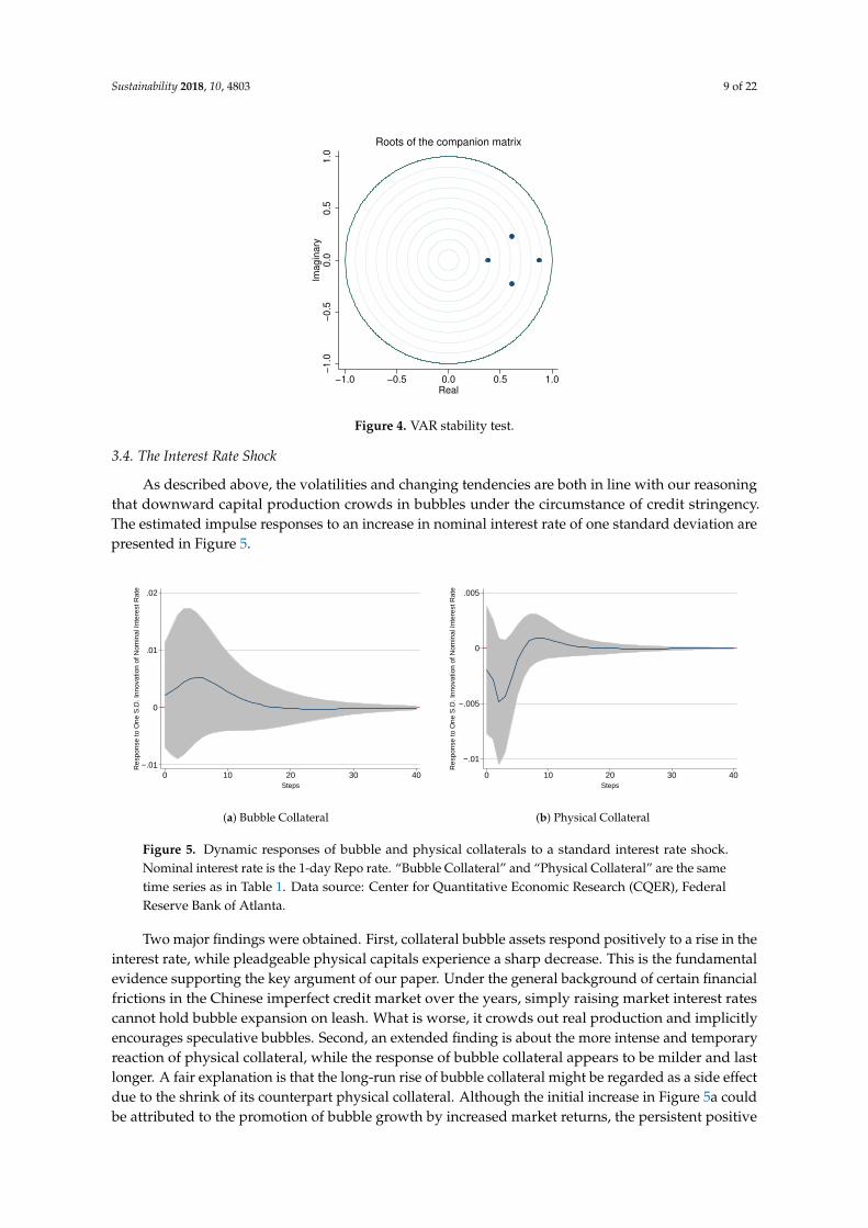
As described above, the volatilities and changing tendencies are both in line with our reasoningthat downward capital production crowds in bubbles under the circumstance of credit stringency.The estimated impulse responses to an increase in nominal interest rate of one standard deviation arepresented in Figure 5.

−.01

0

.01

.02

Res

pons

e to

One

S.D

. Inn

ovat

ion

of N

omin

al In

tere

st R

ate

0 10 20 30 40Steps

(a) Bubble Collateral

−.01

−.005

0

.005

Res

pons

e to

One

S.D

. Inn

ovat

ion

of N

omin

al In

tere

st R

ate

0 10 20 30 40Steps

(b) Physical Collateral

Figure 5. Dynamic responses of bubble and physical collaterals to a standard interest rate shock.Nominal interest rate is the 1-day Repo rate. “Bubble Collateral” and “Physical Collateral” are the sametime series as in Table 1. Data source: Center for Quantitative Economic Research (CQER), FederalReserve Bank of Atlanta.

Two major findings were obtained. First, collateral bubble assets respond positively to a rise in theinterest rate, while pleadgeable physical capitals experience a sharp decrease. This is the fundamentalevidence supporting the key argument of our paper. Under the general background of certain financialfrictions in the Chinese imperfect credit market over the years, simply raising market interest ratescannot hold bubble expansion on leash. What is worse, it crowds out real production and implicitlyencourages speculative bubbles. Second, an extended finding is about the more intense and temporaryreaction of physical collateral, while the response of bubble collateral appears to be milder and lastlonger. A fair explanation is that the long-run rise of bubble collateral might be regarded as a side effectdue to the shrink of its counterpart physical collateral. Although the initial increase in Figure 5a couldbe attributed to the promotion of bubble growth by increased market returns, the persistent positive

Sustainability 2018, 10, 4803 10 of 22

impact discloses an indirect consequence brought by other factors in the whole system. In addition,the narrow grey area of confidence intervals in Figure 5b from a different aspect indicates the directand significant response of physical collateral.

As a whole, the VAR model provides empirical evidence supporting our deduction of the effectthat an austerity measure depresses general production and restrains capital formation. When investorsfind that their physical assets are not enough to borrow under the stringent liquidity constraint inmortgage markets, they will naturally and inevitably turn to hold more bubbles, especially representedby the residential mortgage, which is more easily obtained with its sound guarantee.

4. Model

4.1. Bubble Formation

Consider a two-period overlapping generation (OLG) model with representative agents of workersand entrepreneurs. We construct rational bubbles in asset markets in the spirit of [12]. Intuitivelymanifested by the soaring housing prices, every young household born at time t is given by naturean intrinsically useless bubble with no endogenous payoff of quantity δ ∈ [0, 1) and price Qt|t ≥ 0.Hence, the aggregate value of the new-created bubbles at period t is defined as Ut = δQt|t.

After the new bubbles held by young agents enter transaction markets, they are all traded actively.The aggregate value of trading bubbles can be expressed as QB

t = ∑∞k=0 Qt|t−kZt|t−k, where Qt|t−k and

Zt|t−k separately denote the current price and quantity of the asset bubble introduced at period t− k,(k = 0, 1, 2, . . . ).

To guarantee that the fluctuations in trade markets are merely driven by the movement ofendogenous prices of bubbles in transaction, we keep the total volume of deals constant by letting thesame quantity δ of bubbles generated in every past period vanish and lose value.

The remaining part QBt −Ut, which is not destroyed by bubble bursting, is intuitively deemed

as the value of “bubble stock” Bt. That is to say, the aggregate value of trading bubbles consists oftwo components, which are newly created bubbles and pre-existing stock: QB

t = Ut + Bt.Apart from buying and selling bubbles in asset markets, every individual participates in the

production process either as a worker providing labor or as an entrepreneur conducting production.Labor is identically and inelastically supplied by young workers who earn real wages Wt. Except forreceiving speculative gains in asset markets, old workers obtain an investment yield, pay backloans borrowed in youth, and then use the remaining money to consume. On the supply side,old entrepreneurs produce wholesale goods and sell them in batch size to young entrepreneurs whooperate retail firms. Revenues of wholesale firms are shared in the whole group of old individualsin proportion to their previous investments made at a young age. Accordingly, retailers differentiatewholesale products and resell to gain excess profits. This design is enlightened by the authors in [47],who construct a growth model with heterogeneous productivity and credit access among firms toexplain stylized features during China’s economic transition.

4.2. Wholesale Firms

Wholesale goods are produced using labor and capital: Yt = Kαt N1−α

t , where α is the input shareof capital. Old entrepreneurs maximize profits:

maxNt

{Yt

X−WtNt

}where X > 1 is the relative price between wholesale and retail goods.

First order conditions give real wages of workers Wt and the value of the firm V(Kt), which isshared proportionally among old agents:

Sustainability 2018, 10, 4803 11 of 22

Wt =1− α

X

(Kt

Nt

)α

(2)

V(Kt) = αX−1α

(1− α

Wt

) 1α−1

Kt ≡ ρEtKt (3)

where ρEt > 0 denote the rate of return on capital. Physical capital is raised by the investment fromyoung generations and suffers no depreciation. At the end of the production process, old entrepreneurssell out Kt to offset consumption.

4.2.1. Collateral Constraints

In order to analyze the function of bubbles as extra financing assets, we consider financial frictionscharacterized by credit constraints consistent with that in [8]. Assume commercial banks purchaseloan contracts from borrowers with limited commitment. Here we simplify banking activities andexclude bankers from the scope of our overlapping generation agents. Young agents borrow Lt backedby collateral compositions of valueless housing bubbles plus tangible firm revenues, and pay backRtLt in old age with real interest rates Rt. At time t, banks earn Mt = Lt − Rt−1Lt−1 for operation andadministration. In the case of risks that are reneged on the contact, banks have legitimate rights toseize a fraction η ∈ (0, 1) of the collaterals at their expected market value if borrowers default on loans.Credit market imperfections bring about enforcement costs associated with the litigation process,creating credit constraints whereby borrowers cannot completely pledge their feasible collaterals:

Lt ≤η

RtEt

[(1− δ)

∞

∑k=0

Qt+1|t−kZt|t−k + ρEt+1Kt+1

](4)

where η measures the degree of financial frictions, which signifies perfect borrowing markets when itconverges to one.

4.3. Retail Firms

Young entrepreneurs (retailers) purchase wholesale goods Yt with price 1X , and differentiate and

sell them in a final composite YFt in monopolistically competitive markets, obtaining profits ψt. In the

presence of uncertainty and non-neutral monetary policy, we embed nominal rigidity in the way thatprices are determined before retailer i ∈ [0, 1] buys Yt(i). Therefore, each retailer chooses Pt(i) oneperiod ahead by

maxPt(i)

Et−1

{Λt−1,t

[(Pt(i)

Pt

)Yt(i)−

1X

Yt(i)]}

where Λt−1,t = β(

C2,tC1,t−1

)− 1θ is the stochastic discount factor between t− 1 and t. Retailers are subject

to demand function in the constant elasticity of substitution (CES) form: Yt(i) =(

Pt(i)Pt

)−εYF

t , where

ε is the price elasticity and 1X = ε−1

ε indicates markup. In equilibrium, the optimal price settingP∗t (i) satisfies

βEt−1

{(C2,t

C1,t−1

)− 1θ YF

tPt

(P∗t (i)

Pt

)−ε (P∗t (i)Pt− 1)}

= 0 (5)

4.4. Household

A representative agent born at period t maximizes his or her lifetime utility in the constant relativerisk aversion (CRRA) form.

Sustainability 2018, 10, 4803 12 of 22

maxC

1− 1θ

1,t − 1

1− 1θ

+ βEtC

1− 1θ

2,t+1 − 1

1− 1θ

where β is the discount factor, and 1/θ is the risk aversion coefficient. The budget constraints for theagent in the young and old age are, separately,

C1,t +∞

∑k=0

Qt|t−kZt|t−k + Kt+1 = ψt + WtNt + δQt|t + Lt (6)

C2,t+1 + RtLt = ρEt+1Kt+1 + Kt+1 + (1− δ)∞

∑k=0

Qt+1|t−kZt|t−k (7)

where Wt is the wage received, and Lt is the loan in period t. In the old period, the agent repays theloan and consumes all wealth, both the value of the capital and the bubble.

Optimal consumption decisions give expected growth rates of the bubble price and value:

(1− δ)EtQt+1|t−k

Qt|t−k=

EtBt+1

Qt=

1 + (1− η)EtρEt+1ηRt

+ (1− η). (8)

By virtue of our extension of collateralization, bubbles are expected to grow not only with themarket return, but also with the expected rate of return. Provided that EtρEt+1 evolves along with Rt,which is very sensible since higher interest rate restrains productivity and promotes capital return,the bubble growth will be further encouraged. In addition, Equation (8) implicitly reveals the assistantrole of financial frictions in motivating bubbles.

4.5. Monetary Authority

Monetary policy follows a Taylor rule, where interest rates respond to policy inertia with ϕr,output gap with ϕy, and aggregate bubbles with ϕq:

Rt

R∗=

(Rt−1

R∗

)ϕr ( YFt

YF∗

)(1−ϕr)ϕy ( QBt

QB∗

)(1−ϕr)ϕq

ξt (9)

where 0 < ϕr < 1, ϕy > 0 and the sign of ϕq reflects monetary bubble reactions. ξt denotes a monetarypolicy shock following an auto-regressive process with a lag order of one: ln ξt = ρξ ln ξt−1 + ε

ξt , where

0 < ρξ < 1 and εξt ∼ i.i.d.N(0, σ2

ξ ). Inflation is abstracted from the model, which implies real interestrates actually equal nominal interest rates.

4.6. Equilibrium

In equilibrium, goods market clears and labor is nominalized to one:

C1,t + C2,t + It = Mt + YFt (10)

Nt = 1 (11)

where It = Kt+1 − Kt. Bubble assets lasting for k periods are actively traded, which ensures allbubbles held by the young are bought out by their contemporary old generations. As illustrated before,total trade volume is constant: ∑∞

k=0 Zt|t−k = 1.

5. Results and Discussion

5.1. Bubble Steady State

In steady state, equilibrium output Y in a bubble economy is solved by the Euler equation:

Sustainability 2018, 10, 4803 13 of 22

(C1(Y)C2(Y)

)− 1θ

= β

1ρE(Y)

+ (1− η)

1ρE(Y)

− ηR

(12)

where

C1(Y) =[

1 +( η

R− 1)

α

(1− 1

ε

)]Y−Y

1α +

( η

R− 1)

B(Y) (13)

C2(Y) = (1− η)α

(1− 1

ε

)Y + Y

1α + (1− η)B(Y) (14)

ρE(Y) = α

(1− 1

ε

)Y1− 1

α . (15)

Steady-state values of bubble stock and other variables are given by

B(Y) =U [1 + (1− η)ρE(Y)]

η(

1R − 1

)− (1− η)ρE(Y)

(16)

L(Y) =η

R

[α

(1− 1

ε

)Y + B(Y)

](17)

K = Y1α (18)

YF = Y. (19)

Proposition 1. There exists a unique bubble steady state{

Y, C1, C2, ρE, B, L, K, YF} determined by (12)–(19),if the following condition holds:

R <1

1 +1η−1

α(1− 1ε )

. (20)

Proof. See Appendix A.

Proposition 2. Bubble size B(Y) increases with the interest rate R.

Proof. See Appendix B.

This proposition analytically verifies our key argument that asset bubbles will be boosted by theupregulation of nominal interest rates, in this generalized OLG model incorporating financial frictionsand collateral constraints. The expansionary effect of R on B(Y) is reinforced by collateral constraints,as displayed elaborately in numerical analyses later in Sections 5.3 and 5.4. When the centralbank observes a bubble featured by a high price surpassing the original land price plus reasonabletransaction cost, policy makers ought to chew the cud and carefully assess the timing and situation.The widely used “reverse operation” is no longer applicable if it happens that the financial market isundergoing an extensive deleveraging campaign, which means capital-raising bears a credit frictionand investors have limited borrowing capacity. Under this circumstance, a contractionary monetarypolicy of an elevating interest rate restrains production and decelerates capital formation, so economicagents find it more profitable to invest into bubble assets. What is more, since firms find it moredifficult to conduct fundraising activities, they will have a more urgent need to stay afloat by externalfinancing and hold more intangible bubbles as collateral. For this reason, provided the rise of Rshrinks output and the share of classic capital in the mortgage pool, bubbles are peculiarly stimulatedas a counterweight to efficiently supply liquidity.

Sustainability 2018, 10, 4803 14 of 22

5.2. Calibration

Calibrated values of the structural parameters are reported in Table 5, consistent with existingliterature. We fix the discount factor β at 0.991, the capital share parameter α at 0.33, and the coefficientof relative risk aversion 1/θ at 2. Price elasticity ε is set to be 11 so as to match a monopoly markuplevel of 20%. The benchmark parameter of collateral constraints is 0.7, which implies a moderate levelof financial frictions in credit markets. The newly introduced bubble value is nominalized to 1 on thebasis of the magnitude of this dynamic system. The steady-state real interest rate is set to be 0.2 forsatisfying the sufficient condition in Proposition 1. This calibrated value ensures that the condition inProposition 1 still holds when we later lower the financial friction coefficient η to 0.5 with a view todenote a bad credit environment. Monetary policy parameters for past inertia, output, and bubble arein turn calibrated at 0.8, 0.5, and 0.8. The persistence and volatility of the monetary policy shock arestandardized at 0.5 and 0.003, respectively.

Table 5. Calibrated parameters.

Parameter Description Value

β Discount factor 0.991α Capital share 0.33θ Inverse of risk aversion coefficient 0.5ε Elasticity of substitution 11η Collateral constraints parameter 0.7U Steady-state value of new bubbles 1R Steady-state value of real interest rates 0.2ϕr Taylor rule smoothing coefficient 0.8ϕy Taylor rule coefficient for output 0.5ϕq Taylor rule coefficient for bubble 0.8ρξ Auto-correlation coefficient of the monetary policy shock 0.5σξ Standard deviation of the monetary policy shock 0.003

5.3. Comparative Statics Analysis

Now that we obtain the whole calibrated model, this section derives comparative static resultsand makes further exploration for the developing patterns inside collateral composition. As is depictedby the two planes within the three-dimensional space in Figure 6, the evolutions of bubble stock andfirm value under the change of η and R echo the interactions between bubble and physical collateralsin the empirical evidence in Section 3.

Figure 6 reveals critical implications. In accordance with Proposition 2, bubble size expands asR increases. Furthermore, this expansion exacerbates in a frictional market (rising 0.60− 0.24 = 0.36when η = 0.5) compared with a frictionless credit environment (rising 0.28 − 0.12 = 0.16 whenη = 0.9), in line with the explanation of financial accelerator theory by the authors in [38]. When thecollateral constraint binds, bubble collateral expands and pledgeable firm value shrinks simultaneously.The substitution effect inside collateral composition suggests twofold implications: On the one hand,under a given steady-state real interest rate, a more constrained borrowing condition implicitlymotivates investors to purchase bubble assets to cushion themselves from a liquidity crisis. On theother hand, in a credit market with a certain borrowing condition, tight monetary policy crowds outclassical physical capital and crowds in pledgeable bubble correspondingly.

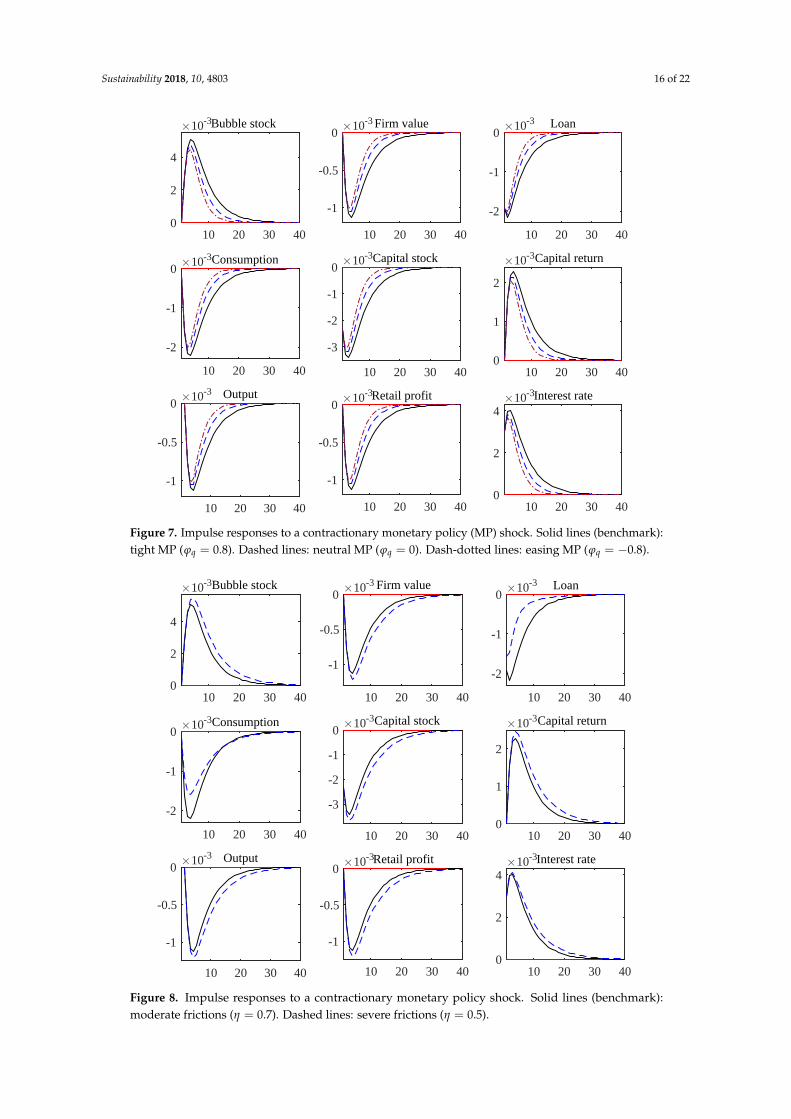
5.4. Impulse Response Analysis

To clarify the mechanisms behind the static results, this section reports the model dynamics,which both corroborate the theoretical application of our model compared with the empirical results inSection 3.4 and strengthen the argument that a tight control of interest rate with an imperfect financialenvironment cannot eliminate the false economic prosperity.

Sustainability 2018, 10, 4803 15 of 22

Figure 6. Comparative statics of collateral composition. “Physical Collateral” denotes a firm value inour model, and the “Bubble Collateral” is the value of bubble stock accordingly.

5.4.1. Benchmark Dynamics

As is depicted in Figures 7 and 8, the simulated model dynamics are highly consistent withthe stylized facts shown in Section 3. A temporary increase in interest rate lifts up borrowing costsand depresses credit and investment, followed by successive downturns in productivity and capitalaccumulation. Consumption and retail profit fall likewise. Bubble collateral (bubble stock) is inflatedrapidly, reflecting a short-term negative impact by the unexpected interest rate increase. Notice thatthe development of collateral bubbles in the meantime crowds out physical collateral (firm values) inthe investor mortgage portfolio.

5.4.2. Monetary Bubble Reactions

The effects of monetary policy design towards market exuberance are shown in Figure 7respectively by the black/blue/crimson lines representing tight/neutral/easing policy measures.A monetary austerity indeed evokes the most violent fluctuations and induces a heavy impact onbubbles to the utmost. Shocks on other core macroeconomic variables are intensified by the same token.

5.4.3. Financial Frictions

Moreover, intuitively demonstrated in Figure 8, the overall trend from η = 0.7 to η = 0.5 generallymanifests the mechanism of the financial accelerator. Just as we argued and showed in the comparativestatics analysis (Section 5.3) earlier, the aggravation of collateral constraints amplifies impacts onbubbles and related indicators. By contrast, two notable exceptions, traced by blue dashed linescounter to the uniform pattern of other indicators, are instead the smaller negative impacts on loan andconsumption. How do they escape from the influence of the financial accelerator and avoid additionalvolatility caused by an unanticipated interest rate increase? The linchpin of this counter-intuitionoriginates from the acceleration mechanism itself. Due to credit deterioration, the debt standing atthe forefront is directly suppressed. Whereas the drop of η transforms a tiny shock into a big turmoil,the rapidly slumped loan magnitude sufficiently mitigates its negative impact indirectly transmittedfrom depressed productivity. The same logic applies to the less dramatic response of short-termconsumption, which gives the collateral coefficient a rather high weight.

Sustainability 2018, 10, 4803 16 of 22

10 20 30 40

-2

-1

010-3Consumption

10 20 30 400

2

4

10-3Bubble stock

10 20 30 400

2

410-3Interest rate

10 20 30 40

-2

-1

010-3 Loan

10 20 30 40

-1

-0.5

010-3 Output

10 20 30 40

-3

-2

-1

010-3Capital stock

10 20 30 400

1

2

10-3Capital return

10 20 30 40

-1

-0.5

010-3Retail profit

10 20 30 40

-1

-0.5

010-3 Firm value

Figure 7. Impulse responses to a contractionary monetary policy (MP) shock. Solid lines (benchmark):tight MP (ϕq = 0.8). Dashed lines: neutral MP (ϕq = 0). Dash-dotted lines: easing MP (ϕq = −0.8).

10 20 30 40

-2

-1

010-3Consumption

10 20 30 400

2

4

10-3Bubble stock

10 20 30 400

2

410-3Interest rate

10 20 30 40

-2

-1

010-3 Loan

10 20 30 40

-1

-0.5

010-3 Output

10 20 30 40

-3

-2

-1

010-3Capital stock

10 20 30 400

1

2

10-3Capital return

10 20 30 40

-1

-0.5

010-3Retail profit

10 20 30 40

-1

-0.5

010-3 Firm value

Figure 8. Impulse responses to a contractionary monetary policy shock. Solid lines (benchmark):moderate frictions (η = 0.7). Dashed lines: severe frictions (η = 0.5).

Sustainability 2018, 10, 4803 17 of 22

6. Conclusions

In the past decade, China’s unsustainable over-borrowing and over-building have brought forthconflict-filled situations, such as mania in housing markets coexisted with a bulk of excess real estatestock, involuntary demographic migrations coexisted with sky-rocketing household debts, and exposedfinancial vulnerabilities coexisted with an incredible scale of local government debt.

This paper looks into the key challenges facing China’s financial market, investigates theunderlying reason of why tight monetary policy coupled with strict capital control is unable toresolve the worrying problems, and puts forward realistic policy implications guiding the steadyand sound development in financial markets, in China but even more so around the whole world,especially at a time with the ongoing downward pressure from escalating trade war.

In a first step, in order to provide a comprehensive overview of the contradiction betweenpersistently growing bubbles and elaborately designed regulatory methods, we collect the latestempirical evidence characterizing the salient features of collateral composition, which comprisesinherently valueless bubble and classic physical capital. Quarterly China’s time series over the pastyears distinctly describe the strikingly high volatility of collateral bubble as well as its negativerelationship with economic output. Apart from this, the VAR results show that, when the financialmarket is exposed to a standard interest rate shock, physical collateral suffers a direct and significantdecline that does not last long, whereas its counterpart (bubble collateral) receives a continuedmoderate promotion. These findings substantiate our argument that rigid interest rate control depressesproductivity and meanwhile encourages asset bubbles.

So as to explore the intrinsic mechanism of how these two collaterals evolve and interact witheach other under certain collocation of monetary control and market pressure, this paper goes a stepfurther to develop a generalized OLG model considering an imperfect market environment in thepresence of limited commitment and insufficient liquidity. Under the constraint that investors canonly receive a small amount of money from their pledged asset value, they have strong incentives toexpand investment by off-balance sheet financing. Even worse, when commercial banks are requiredhigher capital requirements or loan-to-deposit ratios (which are measured by the financial frictioncoefficient η in our model), borrowers are in a more difficult position and rely more on unsustainablespeculative bubbles to resolve the liquidity crisis.

In our specific model design, mathematical proofs justify the unique existence of a bubblyequilibrium, which implies that rational asset bubbles remain at a constant level under a reasonableinterest rate. Moreover, the steady-state bubble size expands when the interest rate increases. After wecalibrate the relevant parameters in accordance with existing literature and Chinese characteristics,we come up with numerical results further illustrating the collateral interactions and model dynamicsbehind the above manifestations. From the comparative static analysis in Section 5.3, either thetightening of monetary control on R or the aggravation of credit condition on η fosters bubble escalationand slows down economic growth at the same time. As the physical capital drops with contractionarymeasures, the pledgeable bubble asset instead rises up to cover the deficit in investor’s mortgageportfolio. Furthermore, from the impulse response analysis, the dynamic evolution in Section 5.4indicates that an unanticipated interest rate rise indeed brings about an inflation effect on the bubble.In addition, deteriorated borrowing friction plays a prominent role as financial accelerator, magnifyingthe aforementioned expansionary effect to a higher level.

6.1. Policy Implications

Finally, we summarize some policy implications on the grounds of our research above.First and foremost, the policy collocation of rigorous monetary control and drastic deleveraging

campaign is not desirable allowing for non-ignorable frictions in financial markets. From asecond thought, China has been fortunate enough to step in a continuous process of the crediblemarket-oriented reform backed by aggressive macroeconomic stimulus and guaranteed politicalstability, for which its housing bubbles have thus far not provoked overturning consequences. Sadly,

Sustainability 2018, 10, 4803 18 of 22

the situation is more grim. In particular, for those even less developed countries or economies withan imperfect capital market, in which asymmetric information and limited commitment give rise tothe problem of credit rationing, insufficient investment caused by funds shortage forces productiveenterprises to reduce production and even close down. In consequence, ordinary residents cannot butshift assets to a redundant housing market, finally leading to a tremendous amount of bubble anddisaster-ridden household debt.

Our second implication is conditional. If and when the collateral constraint in a credit market isalleviated (due to, for example, more transparent information or less default possibility), the centralbank is supposed to step up to fulfill its duty and apply an interest rate tool in a flexible way.This inference gives rise to a more profound conclusion: Given that the decision of financial regulatorsand supervisors on the tightness of credit constraint η always involves a trade-off between thestabilization in asset markets and that in production markets (shown by the impulse response analysisin Section 5.4.3), it is preferable (provided all other conditions are equal) to salvage the social productionat the first place, because at the very least, this decision leaves more policy space for monetaryauthorities to put their multiple instruments to good use.

In addition, a more conceptual element we should ponder over is the intrinsic attribute of realestate bubbles. In light of the inseparable relationship between market prices of land property and itsadditional values from future sale and original agriculture use, the broadly used income approachmethod might not be applicable for analyzing the real estate market, as is examined in detail by theauthors in [48]. The fundamental value derived from the present value formula is not often indicativeof the house property market, and the government need not overreact to the seemingly unexplainedprice premium within a controllable range. Other factors including transaction costs, the risk preferenceof home-buyers, and market expectations all form the real estate price with composite effects.

Last but not the least from the angle of credit transmission, the potential competence of monetarypolicy to surmount its major obstacle is expected to be restored if efficient macro prudential regulationsprevent the formation of a positive feedback loop between bubbles and credit supply. Given thediversification and flexibility of their extended tool set as well as the rear position they are standing at,regulatory institutions have the desirability and feasibility to rupture the unsustainable relationshipbetween bubble and credit, freeing the powerful effect of the interest rate policy.

6.2. Limitations and Future Research

With a view to maintaining the sound and durable real estate market, which is quite essentialto improve people’s life quality, enable common residents to settle down peacefully, and ultimatelyrealize a harmonious and stable society, a monetary policy that is too harsh is not recommended.A housing bubble associated with many derivative problems has become a troublesome issue in publicdebate since the subprime crisis, and this paper merely proceeds from the perspective of a collateralmechanism and provides fresh insight into the possibly appropriate policy measures. In a futurestudy, we are interested in subdividing the households who hold real estate bubbles into age-specificheterogeneous groups. A more intricate design for more responsive young home-buyers is beyond thelength of this article, but this could be a realistic and meaningful exploration for assessing the effectsof demographic developments as well as an ageing population. In addition, another valuable researchdirection is to evaluate the environmental side effects of the twofold austerity campaign on price andon credit. Inspiring research has recently carefully and rigorously considered environmental and socialcharacteristics: Using analytic hierarchy process (AHP) methodology on account of environmentalfactors such as urban clusters and rural grid cells, the authors in [49] propose a precise assessment ofthe sophisticated development trends in the Euro Area. They comprehensive studied the real estatemarket and made a convincing case of the potential necessity of a transition to modernized and newlyconstructed real estate portfolios. Similarly paying attention to the macroeconomic constraints on theoperation and evolution of farmland assets, the authors in [50] emphasize the social and ecologicalvalues that have been greatly underestimated in the potential values of farmland in China. Under this

Sustainability 2018, 10, 4803 19 of 22

circumstance, the deep relationships between house price, land reallocation, an ageing population,and residential structure are worth exploring. In the case of a dismal outlook on the housing marketand an even worse financing environment, a rational real estate agency is very likely to sell off, leavinga bulk of abandoned and unfinished buildings. Dozens of uncompleted residential flats are extremelyharmful to the sustainability of cultivated land and a balanced ecosystem and result in serious scarcityin nature and the environment.

Author Contributions: Q.Y.Y. developed the study concept, conducted the empirical and theoretical analyses,and wrote the paper. Y.Z.L. contributed the theoretical part, produced mathematical proofs, and revised the paper.C.S.X. contributed research methodology, polished the introduction, and revised the paper.

Funding: This work was financially supported by the National Social Science Fund of China (Major Program.Grant No. 08&ZD037).

Acknowledgments: We want to thank the reviewers for their helpful comments and suggestions, which improvedthe paper.

Conflicts of Interest: The authors declare no conflict of interest. The funders had no role in the design of thestudy; in the collection, analyses, or interpretation of data; in the writing of the manuscript; or in the decision topublish the results.

Appendix A. Proof of Proposition 1

For a well-defined bubble steady state{

Y, C1, C2, ρE, B, L, K, YF} determined by

Equations (12)–(19), we have B > 0, ρbE > 0 and C1 > 0, indicating that ρE <

{Rη ,

1R−11η−1

}and R < 1.

Rearranging Euler Equation, we obtain that

F(ρE) =C1(ρE)

C2(ρE)−(

β

1ρE

+ (1− η)

1ρE− η

R

)−θ

. (A1)

We only need to prove that F(ρE) = 0 has a unique solution in (0, ρ), where ρ is the upperbound of ρE. (In the strict sense, it should be a closed interval [0, ρ] in order to apply the property ofcontinuous function in a closed interval. However, we can pin down the values to keep the continuityat F(0) = limρE→0+ F(ρE) = 0 and F(ρ) = limρE→ρ− F(ρE).)

For R < η,Rη<

1R − 11η − 1

, (A2)

which implies ρE < R/η. Using the adjoint of Equations (13) and (14), it immediately follows thatlim

ρE→0+F(ρE) < 0 and lim

ρE→(R/η)−F(ρE) > 0. Next, we derive the sufficient condition to keep the

monotonicity of F(ρE). For the first term in the right-hand side of Equation (A1), differentiatingEquations (13) and (14) with respect to ρE yields

d ln (C1/C2)

d ln ρE

=

{[1 +

( ηR − 1

)A]

YC1

− Y1α

αC1− (1− η)AY

C2− Y

1α

αC2

}d ln Yd ln ρE

+

{( ηR − 1

)B

C1− (1− η)B

C2

}d ln Bd ln ρE

=G(Y)d ln Yd ln ρE

+

(ηR − 1

C1− 1− η

C2

)B

d ln Bd ln ρE

Sustainability 2018, 10, 4803 20 of 22

where G(Y) =[1+( η

R−1)α(1− 1ε )]Y−

1α Y

1α

C1− (1−η)α(1− 1

ε )Y+ 1α Y

1α

C2. From Equations (15) and (16) again,

we obtaind ln Yd ln ρE

=α

α− 1< 0

d ln Bd ln ρE

=(1− η)

[η(

1R − 1

)− (1− η)ρE

]+ (1− η) [1 + (1− η)ρE][

η(

1R − 1

)− (1− η)ρE

]2ρEB

> 0.

Let a = 1 +( η

R − 1)

A and b = (1− η)A. Rearranging G(Y), we obtain that

αC1C2G(Y) =α2C2Y−Y1α C2 − αbC1Y− C1Y

1α

=Y1α +1(αa− b + αb− a) +

[αa(1− η)− αb

( η

R− 1)]

YB−[(1− η) +

( η

R− 1)]

Y1α B

=(α− 1)(a + b)Y1α +1 + α

[a(1− η)− b

( η

R− 1)]

YB−( η

R− η

)Y

1α B

=(α− 1)(a + b)Y1α +1 + α(1− η)YB−

( η

R− η

)Y

1α B

where the fourth equality follows from a(1− η)− b(η/R− 1) = 1− η. Since a + b = 1+ η(1/R− 1)A,the equation above is reduced to

(α− 1)(a + b)Y1α +1 + α(1− η)YB−

( η

R− η

)Y

1α B

=(α− 1)[

1 + η

(1R− 1)

A]

Y1α +1 + α(1− η)YB− η

(1R− 1)

Y1α B

=(α− 1)[

1 + η

(1R− 1)

A]

Y1α +1 + YB

[α(1− η)− η

(1R− 1)

Y1α−1]

=(α− 1)[

1 + η

(1R− 1)

A]

Y1α +1 + YB

α(1− η)− η

(1R− 1) α

(1− 1

ε

)ρE

< 0

.

Hence, the condition of R < 1

1+1η −1

α(1− 1ε )

ensures G(Y) < 0 and( η

R − 1)− (1− η) > 0, which implies

∂ ln(C1/C2)∂ ln ρE

> 0. Therefore, F(ρE) is monotonously increasing in(

0, Rη

), and the bubble equilibrium is

uniquely determined.

Appendix B. Proof of Proposition 2

Differentiating (12) with respect to R yields that

G̃(Y)d ln Yd ln R

+

[( ηR − 1

)B

C1− (1− η)B

C2

]d ln Bd ln R

=ηR

1ρE− η

R(A3)

where

G̃(Y) = G(Y)− α

(1− 1

ε

)ηY− θ

1− α

α

ηR + (1− η)

ρE< 0( η

R − 1)

BC1

− (1− η)BC2

> 0.

Since B increases in ρE and Y decreases in ρE, it follows that d ln Y/ d ln B < 0 and immediatelyyields that d ln B/ d ln R > 0.

Sustainability 2018, 10, 4803 21 of 22

References

1. Chen, K.; Higgins, P.; Waggoner, D.F.; Zha, T. Impacts of Monetary Stimulus on Credit Allocation andMacroeconomy: Evidence from China; Working Paper 22650; National Bureau of Economic Research:Cambridge, USA, 2016; doi:10.3386/w22650.

2. Iacoviello, M. House prices, borrowing constraints, and monetary policy in the business cycle. Am. Econ. Rev.2005, 95, 739–764. [CrossRef]

3. Poterba, J.M.; Weil, D.N.; Shiller, R. House price dynamics: The role of tax policy and demography. Brook. Pap.Econ. Act. 1991, 1991, 143–203. [CrossRef]

4. Brunnermeier, M.K.; Julliard, C. Money illusion and housing frenzies. Rev. Financ. Stud. 2008, 21, 135–180.[CrossRef]

5. Genesove, D.; Han, L. Search and matching in the housing market. J. Urban Econ. 2012, 72, 31–45. [CrossRef]6. Farhi, E.; Tirole, J. Bubbly liquidity. Rev. Financ. Stud. 2011, 79, 678–706. [CrossRef]7. Martin, A.; Ventura, J. Economic growth with bubbles. Am. Econ. Rev. 2012, 102, 3033–3058. [CrossRef]8. Martin, A.; Ventura, J. Managing credit bubbles. J. Eur. Econ. Assoc. 2016, 14, 753–789. [CrossRef]9. Wang, P.; Wen, Y. Speculative bubbles and financial crises. Am. Econ. J. Macroecon. 2012, 4, 184–221.

[CrossRef]10. Miao, J.; Wang, P. Bubbles and Total Factor Productivity. Am. Econ. Rev. 2012, 102, 82–87. [CrossRef]11. Miao, J.; Wang, P. Asset bubbles and credit constraints. Am. Econ. Rev. 2018, 108, 2590–2628. [CrossRef]12. Galí, J. Monetary policy and rational asset price bubbles. Am. Econ. Rev. 2014, 104, 721–752. [CrossRef]13. Tirole, J. Asset bubbles and overlapping generations. Econometrica 1985, 53, 1499–1528. [CrossRef]14. Glaeser, E.L.; Gyourko, J.; Saiz, A. Housing Supply and Housing Bubbles; Working Paper 14193; National

Bureau of Economic Research: Cambridge, USA, 2008; doi:10.3386/w14193.15. Goodhart, C.A. Price stability and financial fragility. In Financial Stability in a Changing Environment; Palgrave

Macmillan: London, UK, 1995; pp. 439–509. doi:10.1007/978-1-349-13352-9_11.16. Kent, C.; Lowe, P. Asset-Price Bubbles and Monetary Policy; Reserve Bank of Australia: Sydney, Australia, 1997.17. Cecchetti, S.G.; Genberg, H.; Lipsky, J.; Wadhwani, S. Asset Prices and Central Bank Policy; Geneva Reports on

the World Economy; International Center for Monetary and Banking Studies: Geneva, Switzerland, 2000.18. Pesce, M.A. Transmission Mechanisms for Monetary Policy in Emerging Market Economies: What Is New? Technical

Report 35; Bank for International Settlements: Basel, Switzerland, 2008.19. Chow, H.K.; Choy, K.M. Monetary policy and asset prices in a small open economy: A factor-augmented

VAR analysis for Singapore. Ann. Financ. Econ. 2009, 5, 1–23. [CrossRef]20. Smets, F.; Wouters, R. Shocks and frictions in US business cycles: A Bayesian DSGE approach. Am. Econ. Rev.

2007, 97, 586–606. [CrossRef]21. Olsen, Ø. Integrating Financial Stability and Monetary Policy Analysis. Speech at the London School of

Economics, 27 April 2015. Available online: https://www.norges-bank.no/ (accessed on 16 December 2018).22. Gourio, F.; Kashyap, A.K.; Sim, J.W. The trade offs in Leaning Against the Wind. IMF Econ. Rev. 2018,

66, 70–115. [CrossRef]23. Miao, J.; Shen, Z.; Wang, P. Monetary policy and rational asset price bubbles: Comment. Am. Econ. Rev.

2018. forthcoming.24. Bernanke, B.S.; Gertler, M. Monetary Policy and Asset Price Volatility; Working Paper 7559; National Bureau of

Economic Research: Cambridge, USA, 2000; doi:10.3386/w7559.25. Bernanke, B.S.; Gertler, M. Should central banks respond to movements in asset prices? Am. Econ. Rev. 2001,

91, 253–257. [CrossRef]26. Reinhart, V. Planning to Protect Against Asset Bubbles; Hunter, K., Pomerleano, Eds.; Asset Price Bubble;

The MIT Press: Cambridge, MA, USA, 2003; pp. 553–560.27. Mishkin, F.S. How should we respond to asset price bubbles? Financ. Stabil. Rev. 2008, 12, 65–74.28. Conefrey, T.; Gerald, J.F. Managing housing bubbles in regional economies under EMU: Ireland and Spain.

Natl. Inst. Econ. Rev. 2010, 211, 91–108. [CrossRef]29. Farley, J.; Burke, M.; Flomenhoft, G.; Kelly, B.; Murray, D.F.; Posner, S.; Putnam, M.; Scanlan, A.; Witham, A.

Monetary and fiscal policies for a finite planet. Sustainability 2013, 5, 2802–2826. [CrossRef]30. Galí, J.; Gambetti, L. The effects of monetary policy on stock market bubbles: Some evidence. Am. Econ.

J. Macroecon. 2015, 7, 233–57. [CrossRef]

Sustainability 2018, 10, 4803 22 of 22

31. Brunnermeier, M.; Schnabel, I. Bubbles and central banks: Historical perspectives. In Central Banks ata Crossroads: What Can We Learn from History? Number 10528; Cambridge University Press: Cambridge,UK, 2015.

32. Svensson, L.E. Cost-benefit analysis of Leaning Against the Wind. J. Monet. Econ. 2017, 90, 193–213.[CrossRef]

33. Juselius, M.; Borio, C.E.; Disyatat, P.; Drehmann, M. Monetary policy, the financial cycle and ultra-lowinterest rates. Int. J. Cent. Bank. 2017, 13, 55–89.

34. Fisher, I. The debt-deflation theory of great depressions. Econometrica 1933, 1, 337–357. [CrossRef]35. Bernanke, B.S.; Gertler, M. Inside the black box: The credit channel of monetary policy transmission.

J. Econ. Perspect. 1995, 9, 27–48. [CrossRef]36. Kiyotaki, N.; Moore, J. Credit cycles. J. Polit. Econ. 1997, 105, 211–248. [CrossRef]37. Carlstrom, C.T.; Fuerst, T.S. Agency costs, net worth, and business fluctuations: A computable general

equilibrium analysis. Am. Econ. Rev. 1997, 87, 893–910. [CrossRef]38. Bernanke, B.S.; Gertler, M.; Gilchrist, S. The financial accelerator in a quantitative business cycle framework.

In Handbook of Macroeconomics; Elsevier: Amsterdam, The Netherlands, 1999; Volume 1, pp. 1341–1393.doi:10.1016/S1574-0048(99)10034-X.

39. Kocherlakota, N. Bursting bubbles: Consequences and cures. In Proceedings of the Macroeconomicand Policy Challenges Following Financial Meltdowns Conference, Washington, DC, USA, 3 April 2009.Available online: https://www.imf.org/external/np/seminars/eng/2009/macro/index.htm/ (accessed on10 December 2018).

40. Jermann, U.; Quadrini, V. Macroeconomic effects of financial shocks. Am. Econ. Rev. 2012, 102, 238–271.[CrossRef]

41. Miao, J.; Wang, P. Sectoral bubbles, misallocation, and endogenous growth. J. Math. Econ. 2014, 53, 153–163.[CrossRef]

42. Chen, K.; Ren, J.; Zha, T. The nexus of monetary policy and shadow banking in China. Am. Econ. Rev. 2018,in press. [CrossRef]

43. Allen, F.; Barlevy, G.; Gale, D. A Theoretical Model of Leaning against the Wind; Federal Reserve Bank ofChicago Working Paper; Federal Reserve Bank of Chicago: Chicago, IL, USA, 2017.

44. Chang, C.; Chen, K.; Waggoner, D.F.; Zha, T. Trends and cycles in China’s macroeconomy. NBER Macroecon.Annu. 2016, 30, 1–84. [CrossRef]

45. Kaplan, G.; Violante, G.L.; Weidner, J. The wealthy hand-to-mouth. Brook. Pap. Econ. Act. 2014, 77–153.[CrossRef]

46. Lútkepohl, H. New Introduction to Multiple Time Series Analysis; Springer Science & Business Media:Berlin/Heidelberg, Germany, 2005.

47. Song, Z.; Storesletten, K.; Zilibotti, F. Growing like China. Am. Econ. Rev. 2011, 101, 196–233. [CrossRef]48. Del Río, B.S.G.; Perez-Salas, J.; Cervello-Royo, R. Land value and returns on farmlands: An analysis by

Spanish autonomous regions. Span. J. Agric. Res. 2012, 10, 271–280. [CrossRef]49. Cervelló-Royo, R.; Guijarro, F.; Pfahler, T.; Preuss, M. An Analytic Hierarchy Process (AHP) framework for

property valuation to identify the ideal 2050 portfolio mixes in EU-27 countries with shrinking populations.Qual. Quant. 2016, 50, 2313–2329. [CrossRef]

50. Hu, R.; Qiu, D.C.; Xie, D.T.; Wang, X.Y.; Zhang, L. Assessing the real value of farmland in China. J. Mt. Sci.2014, 11, 1218–1230. [CrossRef]

c© 2018 by the authors. Licensee MDPI, Basel, Switzerland. This article is an open accessarticle distributed under the terms and conditions of the Creative Commons Attribution(CC BY) license (http://creativecommons.org/licenses/by/4.0/).