is spatial information in ict data reliable? - arxiv.org · is spatial information in ict data...
TRANSCRIPT

Is spatial information in ICT data reliable?
Maxime Lenormand,1, ∗ Thomas Louail,2, 3 Marc Barthelemy,4, 5 and Jose J. Ramasco2
1Irstea, UMR TETIS, 500 rue Francois Breton, FR-34093 Montpellier, France2Instituto de Fısica Interdisciplinar y Sistemas Complejos IFISC (CSIC-UIB),
Campus UIB, ES-07122 Palma de Mallorca, Spain3CNRS, UMR 8504 Geographie-Cites, 13 rue du four, FR-75006 Paris, France
4Institut de Physique Theorique, CEA-CNRS (URA 2306), FR-91191, Gif-sur-Yvette, France5CAMS, EHESS-CNRS (UMR 8557), 190-198 avenue de France, FR-75013 Paris, France
An increasing number of human activities are studied using data produced by individuals’ ICTdevices. In particular, when ICT data contain spatial information, they represent an invaluablesource for analyzing urban dynamics. However, there have been relatively few contributions inves-tigating the robustness of this type of results against fluctuations of data characteristics. Here, wepresent a stability analysis of higher-level information extracted from mobile phone data passivelyproduced during an entire year by 9 million individuals in Senegal. We focus on two information-retrieval tasks: (a) the identification of land use in the region of Dakar from the temporal rhythmsof the communication activity; (b) the identification of home and work locations of anonymizedindividuals, which enable to construct Origin-Destination (OD) matrices of commuting flows. Ouranalysis reveal that the uncertainty of results highly depends on the sample size, the scale and theperiod of the year at which the data were gathered. Nevertheless, the spatial distributions of landuse computed for different samples are remarkably robust: on average, we observe more than 75%of shared surface area between the different spatial partitions when considering activity of at least100,000 users whatever the scale. The OD matrix is less stable and depends on the scale with ashare of at least 75% of commuters in common when considering all types of flows constructed fromthe home-work locations of 100,000 users. For both tasks, better results can be obtained at largerlevels of aggregation or by considering more users. These results confirm that ICT data are veryuseful sources for the spatial analysis of urban systems, but that their reliability should in generalbe tested more thoroughly.
INTRODUCTION
Massive amounts of geolocalized data are passivelyand continuously produced by individuals when theyuse their mobile devices: smart phones, credit cards,GPSs, RFIDs or remote sensing devices. This del-uge of digital footprints is growing at an extremelyfast pace and represents an unprecedented opportu-nity for researchers, to address quantitatively chal-lenging questions, in the hope of unveiling new in-sights on the dynamics of human societies. Manyfields are concerned by the development of new tech-niques to handle these vast datasets, and range fromapplied mathematics, physics, to computer science,with plenty of applications to a variety of disciplinessuch as medicine, public health and social sciences forexample.
Although data resulting from the use of informa-tion and communications technologies (ICT) have theadvantage of large samples sizes (millions of observa-tions), and high spatio-temporal resolution, they alsoraise new challenging issues. Some are technical andrelated to the storage, management and processing ofthese data [1], while others are methodological, suchas the statistical validity of analysis performed on suchdata. For example, in the case of mobile phone data,researchers have often no control and limited informa-tion regarding the data collection process, which obvi-ously deserves other purposes than scientific research.
∗ Corresponding author: [email protected]
Various hidden biases can affect these data used tostudy the spatial behavior of anonymized individu-als, and consequently observing the world through thelenses of ICT data may therefore lead to possible dis-tortions and erroneous conclusions [2]. It is thus cru-cial to perform statistical tests and to develop meth-ods in order to assess the robustness of the results ob-tained with ICT data. In the research community thatstudies human mobility in urban contexts [3–6], effortsin this sense have been made in recent years, notablyby cross-checking results [7] obtained with ICT dataand with more traditional data sources [7–13]. Thesecomparisons cover different topics, such as the anal-ysis of daily mobility motifs [8], the distribution ofpopulation at different scales [7, 10], the estimation ofcommuting flows [7, 9, 11, 13], and the identificationof land uses [7, 12]. However, the robustness of resultsto sample selection, scale or sample size has, up to ourknowledge, never been studied so far.
In the following, we present two examples of suchuncertainty analysis on higher-level spatial informa-tion extracted from mobile phone metadata, whichwere produced in Senegal in 2013 [14]. We concen-trate on two information-retrieval tasks: first, we eval-uate the uncertainty when inferring land use from therhythms of human communication [15–19]; second, wequantify the uncertainty when identifying individuals’most visited locations [7, 12, 20, 21]. We concludeby mentioning possible future steps in order to assessmore clearly the relevance of various ICT data sourcesfor studying a variety of urban dynamics.
arX
iv:1
609.
0337
5v3
[ph
ysic
s.so
c-ph
] 2
3 N
ov 2
017
2
0.20
0.25
0.30
0.35
0.40
0.45
0.20
0.25
0.30
0.35
0.40
0.45
0.20
0.25
0.30
0.35
0.40
0.45 Residential
0.15
0.20
0.25
0.30
0.35
0.40
0.15
0.20
0.25
0.30
0.35
0.40
0.15
0.20
0.25
0.30
0.35
0.40
Fractionofmobilephoneuser
Business
0.30
0.35
0.40
0.45
0.50
0.55
0.30
0.35
0.40
0.45
0.50
0.55
0.30
0.35
0.40
0.45
0.50
0.55
6 12 18 0 6 12 18 0 6 12 18 0 6 12 18 0 6 12 18 0 6 12 18 0 6 12 18
Nightlife
Time of day
(a) (b)
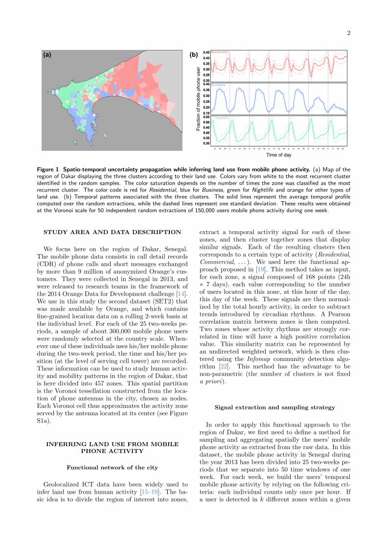
Figure 1. Spatio-temporal uncertainty propagation while inferring land use from mobile phone activity. (a) Map of theregion of Dakar displaying the three clusters according to their land use. Colors vary from white to the most recurrent clusteridentified in the random samples. The color saturation depends on the number of times the zone was classified as the mostrecurrent cluster. The color code is red for Residential, blue for Business, green for Nightlife and orange for other types ofland use. (b) Temporal patterns associated with the three clusters. The solid lines represent the average temporal profilecomputed over the random extractions, while the dashed lines represent one standard deviation. These results were obtainedat the Voronoi scale for 50 independent random extractions of 150,000 users mobile phone activity during one week.
STUDY AREA AND DATA DESCRIPTION
We focus here on the region of Dakar, Senegal.The mobile phone data consists in call detail records(CDR) of phone calls and short messages exchangedby more than 9 million of anonymized Orange’s cus-tomers. They were collected in Senegal in 2013, andwere released to research teams in the framework ofthe 2014 Orange Data for Development challenge [14].We use in this study the second dataset (SET2) thatwas made available by Orange, and which containsfine-grained location data on a rolling 2-week basis atthe individual level. For each of the 25 two-weeks pe-riods, a sample of about 300,000 mobile phone userswere randomly selected at the country scale. When-ever one of these individuals uses his/her mobile phoneduring the two-week period, the time and his/her po-sition (at the level of serving cell tower) are recorded.These information can be used to study human activ-ity and mobility patterns in the region of Dakar, thatis here divided into 457 zones. This spatial partitionis the Voronoi tessellation constructed from the loca-tion of phone antennas in the city, chosen as nodes.Each Voronoi cell thus approximates the activity zoneserved by the antenna located at its center (see FigureS1a).
INFERRING LAND USE FROM MOBILEPHONE ACTIVITY
Functional network of the city
Geolocalized ICT data have been widely used toinfer land use from human activity [15–19]. The ba-sic idea is to divide the region of interest into zones,
extract a temporal activity signal for each of thesezones, and then cluster together zones that displaysimilar signals. Each of the resulting clusters thencorresponds to a certain type of activity (Residential,Commercial, . . . ). We used here the functional ap-proach proposed in [19]. This method takes as input,for each zone, a signal composed of 168 points (24h× 7 days), each value corresponding to the numberof users located in this zone, at this hour of the day,this day of the week. These signals are then normal-ized by the total hourly activity, in order to subtracttrends introduced by circadian rhythms. A Pearsoncorrelation matrix between zones is then computed.Two zones whose activity rhythms are strongly cor-related in time will have a high positive correlationvalue. This similarity matrix can be represented byan undirected weighted network, which is then clus-tered using the Infomap community detection algo-rithm [22]. This method has the advantage to benon-parametric (the number of clusters is not fixeda priori).
Signal extraction and sampling strategy
In order to apply this functional approach to theregion of Dakar, we first need to define a method forsampling and aggregating spatially the users’ mobilephone activity as extracted from the raw data. In thisdataset, the mobile phone activity in Senegal duringthe year 2013 has been divided into 25 two-weeks pe-riods that we separate into 50 time windows of oneweek. For each week, we build the users’ temporalmobile phone activity by relying on the following cri-teria: each individual counts only once per hour. Ifa user is detected in k different zones within a given
3
0
10
20
30
40
50
60
Residential Business Nightlife Other
Per
cent
age
of to
tal s
urfa
ce
Land use type
(a)
60 70 80 90 1000.00
0.05
0.10
0.15
Shared surface area (%)
PD
F
(b)ResidentialBusinessNightlifeTotal
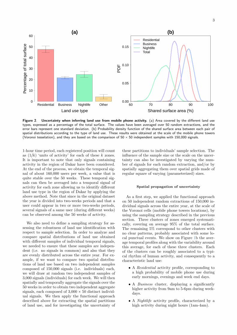
Figure 2. Uncertainty when inferring land use from mobile phone activity. (a) Area covered by the different land usetypes, expressed as a percentage of the total surface. The values have been averaged over 50 random extractions, and theerror bars represent one standard deviation. (b) Probability density function of the shared surface area between each pair ofspatial distributions according to the type of land use. These results were obtained at the scale of the mobile phone towers(Voronoi tesselation), and they are based on the comparison of 50 × 50 independent samples with 150,000 signals.
1-hour time period, each registered position will countas (1/k) ‘units of activity’ for each of these k zones.It is important to note that only signals containingactivity in the region of Dakar have been considered.At the end of the process, we obtain the temporal sig-nal of about 160,000 users per week, a value that isquite stable over the 50 weeks. These temporal sig-nals can then be averaged into a temporal signal ofactivity for each zone allowing us to identify differentland use type in the region of Dakar by applying theabove method. Note that since in the original datasetthe year is divided into two-weeks periods and that auser could appear in two or more two-weeks periods,several signals of a same user (during different weeks)can be observed among the 50 weeks of activity.
We also need to define a sampling strategy for as-sessing the robustness of land use identification withrespect to sample selection. In order to analyze andcompare spatial distributions of land use obtainedwith different samples of individual temporal signals,we needed to ensure that these samples are indepen-dent (i.e. no signals in common) and also that theyare evenly distributed across the entire year. For ex-ample, if we want to compare two spatial distribu-tions of land use based on two independent samplescomposed of 150,000 signals (i.e. individuals) each,we will draw at random two independent samples of3,000 signals (individuals) for each week. We will thenspatially and temporally aggregate the signals over the50 weeks in order to obtain two independent aggregatesignals, each composed of 3,000 × 50 distinct individ-ual signals. We then apply the functional approachdescribed above for extracting the spatial partitionsof land use, and for investigating the uncertainty of
these partitions to individuals’ sample selection. Theinfluence of the sample size or the scale on the uncer-tainty can also be investigated by varying the num-ber of signals for each random extraction, and/or byspatially aggregating them over spatial grids made ofregular square of varying (parameterized) sizes.
Spatial propagation of uncertainty
As a first step, we applied the functional approachon 50 independent random extractions of 150,000 in-dividual signals across the entire year, at the scale ofthe Voronoi cells (mobile phone towers locations), byusing the sampling strategy described in the previoussection. Three clusters of zones emerged systemati-cally, covering on average 95% of the total surface.The remaining 5% correspond to other clusters withno clear patterns, probably associated with some lo-cal punctual events. We show on Figure 1b the aver-age temporal profiles along with the variability aroundthis average, for each of these three clusters. Eachof the clusters can be roughly associated to a typi-cal rhythm of human activity, and consequently to acharacteristic land use:
• A Residential activity profile, corresponding toa high probability of mobile phone use duringearly mornings, evenings and week end days.
• A Business cluster, displaying a significantlyhigher activity from 9am to 5-6pm during week-days.
• A Nightlife activity profile, characterized by ahigh activity during night hours (1am-4am).
4
The Nightlife cluster (in green) covers the area ofthe international airport, and also the neighborhoodof ‘La Pointe des Almadies’, where mainly wealthypeople live and where are located most of the richnightclubs. The Business cluster covers Dakar’s cen-tral business district (‘Le Plateau’ ), where one findscompanies’ headquarters, and where the port is alsolocated. Finally, the Residential cluster covers therapidly growing parts of the Dakar peninsula, whichprofits from the highway construction. It is worthnoting that the different land use types identifiedin this study are consistent with the ones obtainedwith another mobile phone dataset in Spain [19], ex-cept that in the case of Dakar, the method is notable to distinguish between industrial (or logistic) andleisure/nightlife activities (see [19] for more details).
As can be observed in Figure 2a, the area covered bythe different types of land use is quite stable over the50 samples, with the Residential land use type rep-resenting on average about 50% of the total surface,while we observe about 20% and 25% for the Businessand Nightlife clusters, respectively. Nevertheless, thestability of the proportion does not imply that theyfollow the same spatial distribution from one sampleto another. In order to test the stability, we computedthe proportion of surface area shared by two spatialdistributions pl and p′l of a given type l, as obtainedwith two different samples. The expression for thisquantity is
S = 2Apl∩p′l
Apl+Ap′
l
, (1)
where Apldenotes the surface area of spatial distri-
bution pl. Note that in our case Apl≃ Ap′
l(Figure
2a). Similarly, we can define the total surface areashared by two spatial partitions p and p′ (with thesame number and type of land use) of the region ofinterest,
S∗ =∑lApl∩p′l
∑lApl
. (2)
The results are displayed in Figure 2b. The simi-larities between the 50 different spatial partitions isglobally high, with on average 80% of shared surfacearea. The agreement is larger for the Residential andBusiness clusters with an average shared surface areaaround 90%, against 75% for the Nightlife land usetype. This is probably due to the more episodic char-acter of the nightlife activity, implying a smaller sta-tistical reliability of the results. A map of the regionof Dakar displaying the uncertainty associated withthe land use identification is shown in Figure 1a. Thecolors represent the different land use types, and eachzone has been assigned its recurrent cluster type overthe 50 land use identifications. The color saturationis then related to the uncertainty, quantified by thenumber of times the zone was classified as a given re-current cluster: the color is darker if the uncertaintyis low, paler otherwise. Most of the zones have been
assigned to the same clusters more than 80% of thetime.
Influence of scale and sample size on theuncertainty
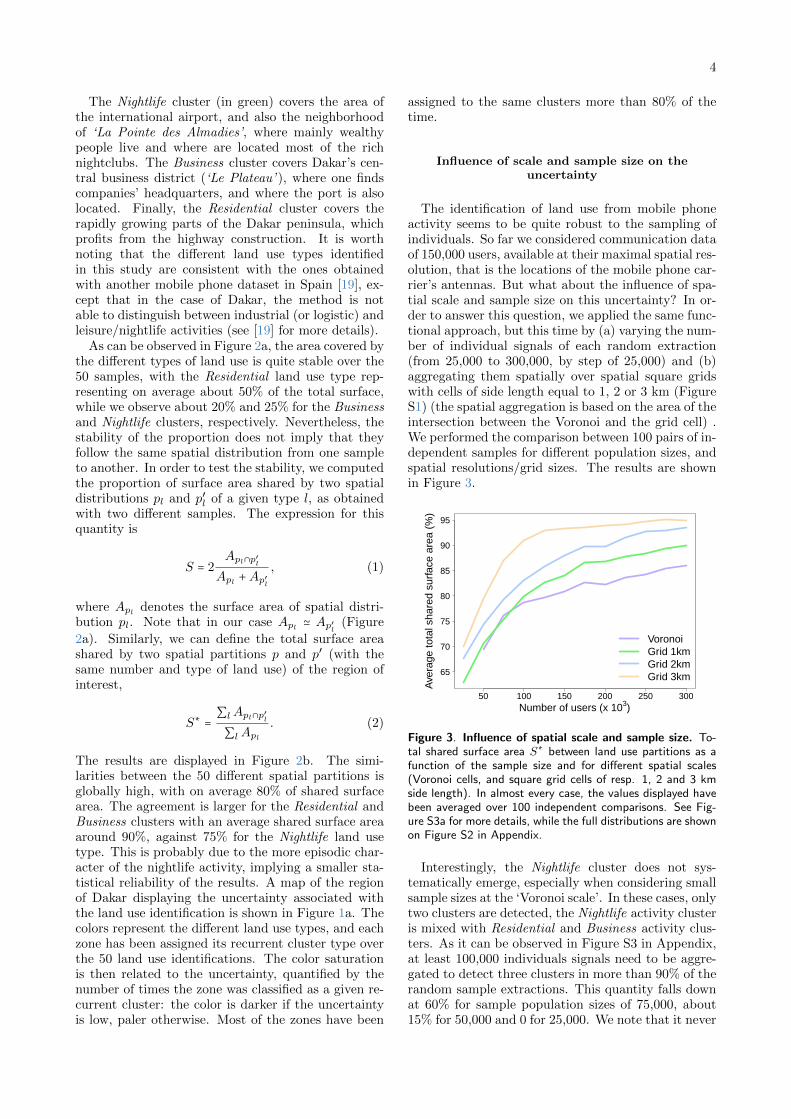
The identification of land use from mobile phoneactivity seems to be quite robust to the sampling ofindividuals. So far we considered communication dataof 150,000 users, available at their maximal spatial res-olution, that is the locations of the mobile phone car-rier’s antennas. But what about the influence of spa-tial scale and sample size on this uncertainty? In or-der to answer this question, we applied the same func-tional approach, but this time by (a) varying the num-ber of individual signals of each random extraction(from 25,000 to 300,000, by step of 25,000) and (b)aggregating them spatially over spatial square gridswith cells of side length equal to 1, 2 or 3 km (FigureS1) (the spatial aggregation is based on the area of theintersection between the Voronoi and the grid cell) .We performed the comparison between 100 pairs of in-dependent samples for different population sizes, andspatial resolutions/grid sizes. The results are shownin Figure 3.
50 100 150 200 250 300
65
70
75
80
85
90
95
Number of users (x 103)
Ave
rage
tota
l sha
red
surf
ace
area
(%
)
VoronoiGrid 1kmGrid 2kmGrid 3km
Figure 3. Influence of spatial scale and sample size. To-tal shared surface area S∗ between land use partitions as afunction of the sample size and for different spatial scales(Voronoi cells, and square grid cells of resp. 1, 2 and 3 kmside length). In almost every case, the values displayed havebeen averaged over 100 independent comparisons. See Fig-ure S3a for more details, while the full distributions are shownon Figure S2 in Appendix.
Interestingly, the Nightlife cluster does not sys-tematically emerge, especially when considering smallsample sizes at the ‘Voronoi scale’. In these cases, onlytwo clusters are detected, the Nightlife activity clusteris mixed with Residential and Business activity clus-ters. As it can be observed in Figure S3 in Appendix,at least 100,000 individuals signals need to be aggre-gated to detect three clusters in more than 90% of therandom sample extractions. This quantity falls downat 60% for sample population sizes of 75,000, about15% for 50,000 and 0 for 25,000. We note that it never
5
happened when the signals have been spatially aggre-gated. Considering only the partitions for which threeclusters were detected, we observe that the percent-age of share surface area increases when the data arespatially coarse-grained, and also with the number ofindividuals taken into account, revealing the existenceof a typical scale. The order of this scale seems to behere of the order 100,000, above which we obtain morethan 75% similarity between the land use spatial par-titions. Coarse-graining the spatial resolution by pro-jecting the data on grids of larger cells plays also animportant role, allowing us to reduce the uncertaintywhen small samples are considered. As expected, thevariability of the uncertainty tends to increase withthe grid cell side length (see Figure S2 in Appendix).
Temporal variations
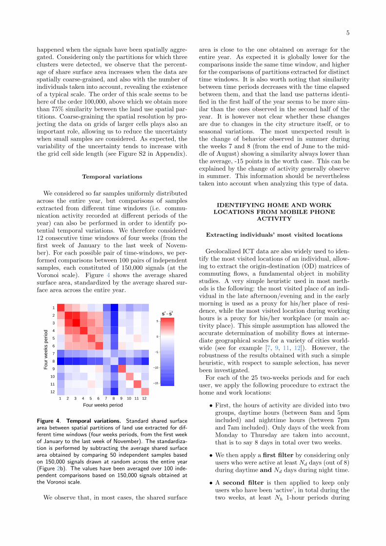
We considered so far samples uniformly distributedacross the entire year, but comparisons of samplesextracted from different time windows (i.e. commu-nication activity recorded at different periods of theyear) can also be performed in order to identify po-tential temporal variations. We therefore considered12 consecutive time windows of four weeks (from thefirst week of January to the last week of Novem-ber). For each possible pair of time-windows, we per-formed comparisons between 100 pairs of independentsamples, each constituted of 150,000 signals (at theVoronoi scale). Figure 4 shows the average sharedsurface area, standardized by the average shared sur-face area across the entire year.
1 2 3 4 5 6 7 8 9 10 11 12
12
11
10
9
8
7
6
5
4
3
2
1
Four weeks period
Fou
r w
eeks
per
iod
−15
−10
−5
0
5
S* − S*
Figure 4. Temporal variations. Standard shared surfacearea between spatial partitions of land use extracted for dif-ferent time windows (four weeks periods, from the first weekof January to the last week of November). The standardiza-tion is performed by subtracting the average shared surfacearea obtained by comparing 50 independent samples basedon 150,000 signals drawn at random across the entire year(Figure 2b). The values have been averaged over 100 inde-pendent comparisons based on 150,000 signals obtained atthe Voronoi scale.
We observe that, in most cases, the shared surface
area is close to the one obtained on average for theentire year. As expected it is globally lower for thecomparisons inside the same time window, and higherfor the comparisons of partitions extracted for distincttime windows. It is also worth noting that similaritybetween time periods decreases with the time elapsedbetween them, and that the land use patterns identi-fied in the first half of the year seems to be more sim-ilar than the ones observed in the second half of theyear. It is however not clear whether these changesare due to changes in the city structure itself, or toseasonal variations. The most unexpected result isthe change of behavior observed in summer duringthe weeks 7 and 8 (from the end of June to the mid-dle of August) showing a similarity always lower thanthe average, -15 points in the worth case. This can beexplained by the change of activity generally observein summer. This information should be neverthelesstaken into account when analyzing this type of data.
IDENTIFYING HOME AND WORKLOCATIONS FROM MOBILE PHONE
ACTIVITY
Extracting individuals’ most visited locations
Geolocalized ICT data are also widely used to iden-tify the most visited locations of an individual, allow-ing to extract the origin-destination (OD) matrices ofcommuting flows, a fundamental object in mobilitystudies. A very simple heuristic used in most meth-ods is the following: the most visited place of an indi-vidual in the late afternoon/evening and in the earlymorning is used as a proxy for his/her place of resi-dence, while the most visited location during workinghours is a proxy for his/her workplace (or main ac-tivity place). This simple assumption has allowed theaccurate determination of mobility flows at interme-diate geographical scales for a variety of cities world-wide (see for example [7, 9, 11, 12]). However, therobustness of the results obtained with such a simpleheuristic, with respect to sample selection, has neverbeen investigated.
For each of the 25 two-weeks periods and for eachuser, we apply the following procedure to extract thehome and work locations:
• First, the hours of activity are divided into twogroups, daytime hours (between 8am and 5pmincluded) and nighttime hours (between 7pmand 7am included). Only days of the week fromMonday to Thursday are taken into account,that is to say 8 days in total over two weeks.
• We then apply a first filter by considering onlyusers who were active at least Nd days (out of 8)during daytime and Nd days during night time.
• A second filter is then applied to keep onlyusers who have been ‘active’, in total during thetwo weeks, at least Nh 1-hour periods during
6
0.2 0.4 0.6 0.8
0
2
4
6
8
10
12
δh
Num
ber
of u
sers
(x
104 )
(a)
Nh ≥ 1Nh ≥ 5Nh ≥ 10Nh ≥ 15Nh ≥ 20
0.2 0.4 0.6 0.8
0.6
0.7
0.8
0.9
1.0
δh
Fra
ctio
n of
intr
a−zo
nal f
low
s
(b)
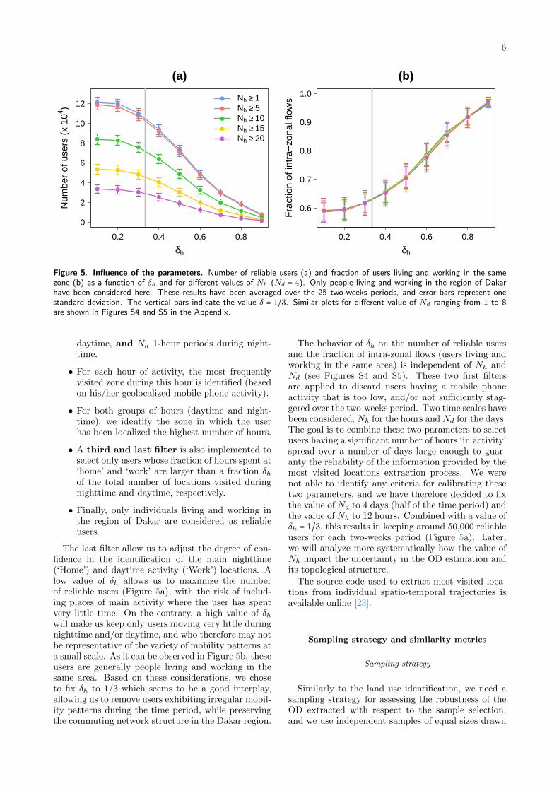
Figure 5. Influence of the parameters. Number of reliable users (a) and fraction of users living and working in the samezone (b) as a function of δh and for different values of Nh (Nd = 4). Only people living and working in the region of Dakarhave been considered here. These results have been averaged over the 25 two-weeks periods, and error bars represent onestandard deviation. The vertical bars indicate the value δ = 1/3. Similar plots for different value of Nd ranging from 1 to 8are shown in Figures S4 and S5 in the Appendix.
daytime, and Nh 1-hour periods during night-time.
• For each hour of activity, the most frequentlyvisited zone during this hour is identified (basedon his/her geolocalized mobile phone activity).
• For both groups of hours (daytime and night-time), we identify the zone in which the userhas been localized the highest number of hours.
• A third and last filter is also implemented toselect only users whose fraction of hours spent at‘home’ and ‘work’ are larger than a fraction δhof the total number of locations visited duringnighttime and daytime, respectively.
• Finally, only individuals living and working inthe region of Dakar are considered as reliableusers.
The last filter allow us to adjust the degree of con-fidence in the identification of the main nighttime(‘Home’) and daytime activity (‘Work’) locations. Alow value of δh allows us to maximize the numberof reliable users (Figure 5a), with the risk of includ-ing places of main activity where the user has spentvery little time. On the contrary, a high value of δhwill make us keep only users moving very little duringnighttime and/or daytime, and who therefore may notbe representative of the variety of mobility patterns ata small scale. As it can be observed in Figure 5b, theseusers are generally people living and working in thesame area. Based on these considerations, we choseto fix δh to 1/3 which seems to be a good interplay,allowing us to remove users exhibiting irregular mobil-ity patterns during the time period, while preservingthe commuting network structure in the Dakar region.
The behavior of δh on the number of reliable usersand the fraction of intra-zonal flows (users living andworking in the same area) is independent of Nh andNd (see Figures S4 and S5). These two first filtersare applied to discard users having a mobile phoneactivity that is too low, and/or not sufficiently stag-gered over the two-weeks period. Two time scales havebeen considered, Nh for the hours and Nd for the days.The goal is to combine these two parameters to selectusers having a significant number of hours ‘in activity’spread over a number of days large enough to guar-anty the reliability of the information provided by themost visited locations extraction process. We werenot able to identify any criteria for calibrating thesetwo parameters, and we have therefore decided to fixthe value of Nd to 4 days (half of the time period) andthe value of Nh to 12 hours. Combined with a value ofδh = 1/3, this results in keeping around 50,000 reliableusers for each two-weeks period (Figure 5a). Later,we will analyze more systematically how the value ofNh impact the uncertainty in the OD estimation andits topological structure.
The source code used to extract most visited loca-tions from individual spatio-temporal trajectories isavailable online [23].
Sampling strategy and similarity metrics
Sampling strategy
Similarly to the land use identification, we need asampling strategy for assessing the robustness of theOD extracted with respect to the sample selection,and we use independent samples of equal sizes drawn

7
0 5 10 15 20 250.786
0.788
0.790
0.792
0.794
0.796
0.798
Nh
λ c
(a)
0 5 10 15 20 25
0.500
0.505
0.510
0.515
0.520
Nh
λ c*
(b)
0 5 10 15 20 25
0.45
0.46
0.47
0.48
0.49
0.50
0.51
Nh
λ l
(c)
0 5 10 15 20 250.994
0.995
0.996
0.997
0.998
0.999
Nh
λ d
(d)
Figure 6. Uncertainty when inferring home-work locations from mobile phone activity. Boxplots of the comparisonsbetween 100 independent ODs according to Nh. (a) λc (all flows). (b) λ∗c (only inter-zonal flows). (c) λl. (d) λd. ODs havebeen extracted at the Voronoi scale from independent samples composed of 150,000 reliable users’ home-work locations (withNd = 4 and δh = 1/3). The whiskers correspond to the minimum and maximum of the distributions.
at random across the 25 two-weeks periods. For exam-ple, for comparing two ODs retrieved from two inde-pendent samples of 150,000 reliable users’ home-worklocations, we draw at random two independent sam-ples of size 6,000 for each of the two-weeks period.Here also, we evaluate the influence of the sample sizeand of the spatial resolution on the uncertainty, byvarying the number of signals extracted at each ran-dom extraction and/or by spatially aggregating thesignals over spatial grids of varying sizes.
Similarity metrics
The resulting commuting networks can be com-pared using several similarity metrics, such as the onedescribed in [24]. We consider two commuting net-works T and T ′, where Tij is the number of usersliving in zone i and working in zone j, and we will usethree different metrics, that encode different networkproperties. First, the common fraction of commuters,noted λc, varying from 0 (when there is no overlap)to 1 (when the two networks are identical) is given by
λc =2∑i,j min(Tij , T ′ij)∑i,j Tij +∑i,j T
′
ij
. (3)
With this first metric, the similarity is calculatedconsidering all flows, without distinction between the
intra-zonal flows and the inter-zonal flows. The firsttype of flows tends to gather a large part of the com-muters distributed over a limited number of linkswhereas the latter are usually less stable and moredifficult to estimate. To take into consideration thesedifferent types of flows we will also consider, as a sim-ilarity metric, the common fraction of commuters, λ∗c ,based only on the users living and working in two dif-ferent places (i ≠ j).
Second, we will consider the common fraction oflinks, λl, that measures similarity in the networks’topological structure, and is calculated as
λl =2∑i,j 1Tij>0 ⋅ 1T ′ij>0
∑i,j 1Tij>0 +∑i,j 1T ′ij>0
. (4)
Third, we measure the common share of commutersaccording to the distance, λd, assessing the similaritybetween commuting distance distributions and givenby
λd =∑k min(Nk,N
′
k)N
, (5)
where Nk stands for the number of users with a com-muting distance ranging between 2k − 2 and 2k kms(k ranging from 1 to ∞) and N for the total numberof users.
8
50 100 150 200 250 3000.65
0.70
0.75
0.80
0.85
0.90
0.95
Number of users (x 103)
λ c
(a)
50 100 150 200 250 300
0.4
0.6
0.8
Number of users (x 103)
λ c*
(b)
50 100 150 200 250 300
0.3
0.4
0.5
0.6
0.7
0.8
0.9
Number of users (x 103)
λ l
(c)
50 100 150 200 250 300
0.994
0.995
0.996
0.997
0.998
Number of users (x 103)
λ l
(d)
VoronoiGrid 1kmGrid 2kmGrid 3km
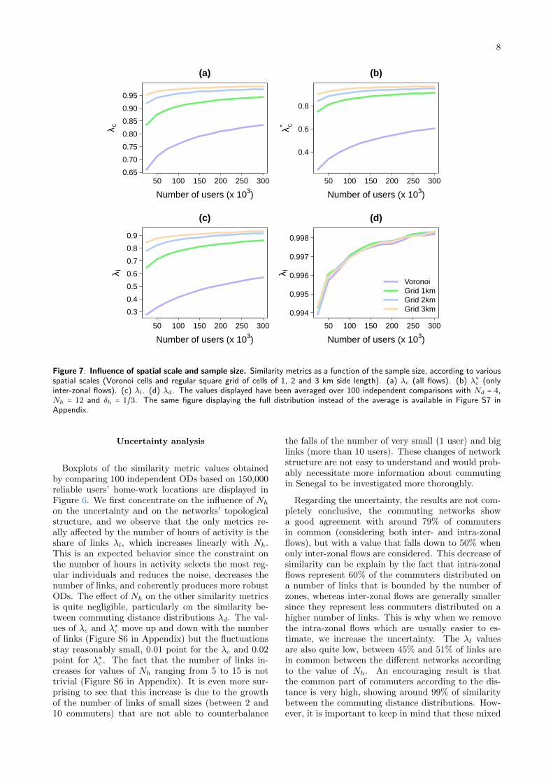
Figure 7. Influence of spatial scale and sample size. Similarity metrics as a function of the sample size, according to variousspatial scales (Voronoi cells and regular square grid of cells of 1, 2 and 3 km side length). (a) λc (all flows). (b) λ∗c (onlyinter-zonal flows). (c) λl. (d) λd. The values displayed have been averaged over 100 independent comparisons with Nd = 4,Nh = 12 and δh = 1/3. The same figure displaying the full distribution instead of the average is available in Figure S7 inAppendix.
Uncertainty analysis
Boxplots of the similarity metric values obtainedby comparing 100 independent ODs based on 150,000reliable users’ home-work locations are displayed inFigure 6. We first concentrate on the influence of Nh
on the uncertainty and on the networks’ topologicalstructure, and we observe that the only metrics re-ally affected by the number of hours of activity is theshare of links λl, which increases linearly with Nh.This is an expected behavior since the constraint onthe number of hours in activity selects the most reg-ular individuals and reduces the noise, decreases thenumber of links, and coherently produces more robustODs. The effect of Nh on the other similarity metricsis quite negligible, particularly on the similarity be-tween commuting distance distributions λd. The val-ues of λc and λ∗c move up and down with the numberof links (Figure S6 in Appendix) but the fluctuationsstay reasonably small, 0.01 point for the λc and 0.02point for λ∗c . The fact that the number of links in-creases for values of Nh ranging from 5 to 15 is nottrivial (Figure S6 in Appendix). It is even more sur-prising to see that this increase is due to the growthof the number of links of small sizes (between 2 and10 commuters) that are not able to counterbalance
the falls of the number of very small (1 user) and biglinks (more than 10 users). These changes of networkstructure are not easy to understand and would prob-ably necessitate more information about commutingin Senegal to be investigated more thoroughly.
Regarding the uncertainty, the results are not com-pletely conclusive, the commuting networks showa good agreement with around 79% of commutersin common (considering both inter- and intra-zonalflows), but with a value that falls down to 50% whenonly inter-zonal flows are considered. This decrease ofsimilarity can be explain by the fact that intra-zonalflows represent 60% of the commuters distributed ona number of links that is bounded by the number ofzones, whereas inter-zonal flows are generally smallersince they represent less commuters distributed on ahigher number of links. This is why when we removethe intra-zonal flows which are usually easier to es-timate, we increase the uncertainty. The λl valuesare also quite low, between 45% and 51% of links arein common between the different networks accordingto the value of Nh. An encouraging result is thatthe common part of commuters according to the dis-tance is very high, showing around 99% of similaritybetween the commuting distance distributions. How-ever, it is important to keep in mind that these mixed
9
results are obtained with a few thousand users for eachtwo-weeks commuting network, drawn at a high spa-tial resolution with an average surface area equal to0.5 km2.
Influence of scale and sample size
The effect of the spatial resolution and sample sizeson the similarity metrics can be investigated by vary-ing the number of reliable users’ home-work most vis-ited locations to build the ODs and/or by aggregatingthem spatially using grid cells of different sizes (see [7]for more details about the aggregation method basedon the area of the intersection between the Voronoiand the grid cells). As it can be observed in Figure7, increasing the sample size and/or the scale greatlyimprove the results. Here again, considering at least100,000 reliable users seems to be a good trade-offand ensure a common part of commuters larger than75%. The most significant improvement comes fromthe spatial aggregation, which at least double λ∗c andλl values and allow us to obtain λc values almost al-ways larger than 0.85. There is one exception, though,with λl that seems to be independent from the spatialaggregation scale used.
Temporal variations
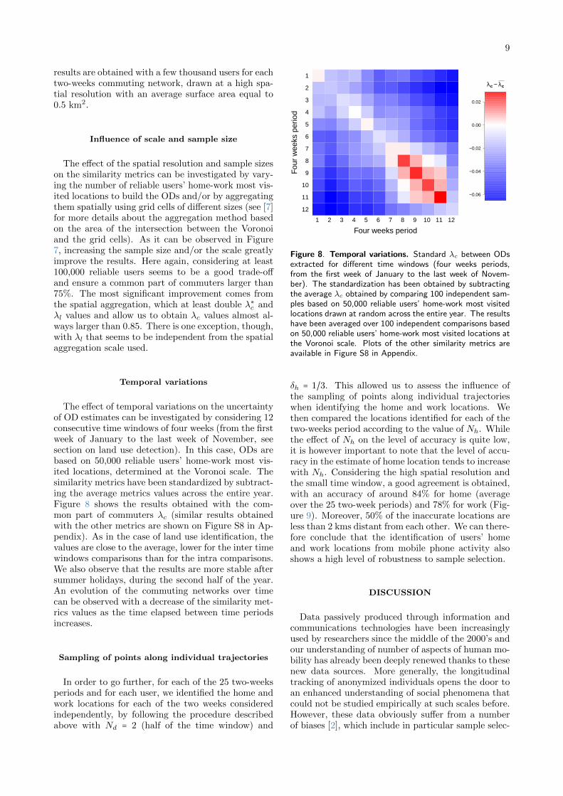
The effect of temporal variations on the uncertaintyof OD estimates can be investigated by considering 12consecutive time windows of four weeks (from the firstweek of January to the last week of November, seesection on land use detection). In this case, ODs arebased on 50,000 reliable users’ home-work most vis-ited locations, determined at the Voronoi scale. Thesimilarity metrics have been standardized by subtract-ing the average metrics values across the entire year.Figure 8 shows the results obtained with the com-mon part of commuters λc (similar results obtainedwith the other metrics are shown on Figure S8 in Ap-pendix). As in the case of land use identification, thevalues are close to the average, lower for the inter timewindows comparisons than for the intra comparisons.We also observe that the results are more stable aftersummer holidays, during the second half of the year.An evolution of the commuting networks over timecan be observed with a decrease of the similarity met-rics values as the time elapsed between time periodsincreases.
Sampling of points along individual trajectories
In order to go further, for each of the 25 two-weeksperiods and for each user, we identified the home andwork locations for each of the two weeks consideredindependently, by following the procedure describedabove with Nd = 2 (half of the time window) and
1 2 3 4 5 6 7 8 9 10 11 12
12
11
10
9
8
7
6
5
4
3
2
1
Four weeks period
Fou
r w
eeks
per
iod
−0.06
−0.04
−0.02
0.00
0.02
λc − λc
Figure 8. Temporal variations. Standard λc between ODsextracted for different time windows (four weeks periods,from the first week of January to the last week of Novem-ber). The standardization has been obtained by subtractingthe average λc obtained by comparing 100 independent sam-ples based on 50,000 reliable users’ home-work most visitedlocations drawn at random across the entire year. The resultshave been averaged over 100 independent comparisons basedon 50,000 reliable users’ home-work most visited locations atthe Voronoi scale. Plots of the other similarity metrics areavailable in Figure S8 in Appendix.
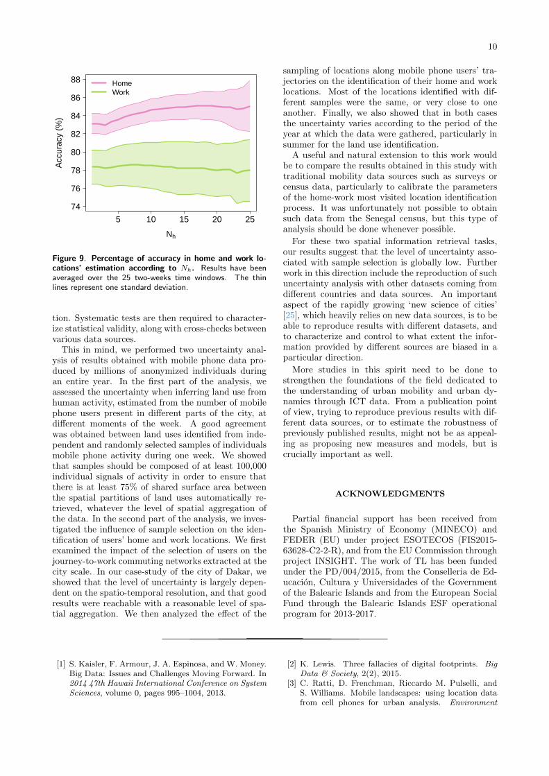
δh = 1/3. This allowed us to assess the influence ofthe sampling of points along individual trajectorieswhen identifying the home and work locations. Wethen compared the locations identified for each of thetwo-weeks period according to the value of Nh. Whilethe effect of Nh on the level of accuracy is quite low,it is however important to note that the level of accu-racy in the estimate of home location tends to increasewith Nh. Considering the high spatial resolution andthe small time window, a good agreement is obtained,with an accuracy of around 84% for home (averageover the 25 two-week periods) and 78% for work (Fig-ure 9). Moreover, 50% of the inaccurate locations areless than 2 kms distant from each other. We can there-fore conclude that the identification of users’ homeand work locations from mobile phone activity alsoshows a high level of robustness to sample selection.
DISCUSSION
Data passively produced through information andcommunications technologies have been increasinglyused by researchers since the middle of the 2000’s andour understanding of number of aspects of human mo-bility has already been deeply renewed thanks to thesenew data sources. More generally, the longitudinaltracking of anonymized individuals opens the door toan enhanced understanding of social phenomena thatcould not be studied empirically at such scales before.However, these data obviously suffer from a numberof biases [2], which include in particular sample selec-
10
5 10 15 20 25
74
76
78
80
82
84
86
88
Nh
Acc
urac
y (%
)
HomeWork
Figure 9. Percentage of accuracy in home and work lo-cations’ estimation according to Nh. Results have beenaveraged over the 25 two-weeks time windows. The thinlines represent one standard deviation.
tion. Systematic tests are then required to character-ize statistical validity, along with cross-checks betweenvarious data sources.
This in mind, we performed two uncertainty anal-ysis of results obtained with mobile phone data pro-duced by millions of anonymized individuals duringan entire year. In the first part of the analysis, weassessed the uncertainty when inferring land use fromhuman activity, estimated from the number of mobilephone users present in different parts of the city, atdifferent moments of the week. A good agreementwas obtained between land uses identified from inde-pendent and randomly selected samples of individualsmobile phone activity during one week. We showedthat samples should be composed of at least 100,000individual signals of activity in order to ensure thatthere is at least 75% of shared surface area betweenthe spatial partitions of land uses automatically re-trieved, whatever the level of spatial aggregation ofthe data. In the second part of the analysis, we inves-tigated the influence of sample selection on the iden-tification of users’ home and work locations. We firstexamined the impact of the selection of users on thejourney-to-work commuting networks extracted at thecity scale. In our case-study of the city of Dakar, weshowed that the level of uncertainty is largely depen-dent on the spatio-temporal resolution, and that goodresults were reachable with a reasonable level of spa-tial aggregation. We then analyzed the effect of the
sampling of locations along mobile phone users’ tra-jectories on the identification of their home and worklocations. Most of the locations identified with dif-ferent samples were the same, or very close to oneanother. Finally, we also showed that in both casesthe uncertainty varies according to the period of theyear at which the data were gathered, particularly insummer for the land use identification.
A useful and natural extension to this work wouldbe to compare the results obtained in this study withtraditional mobility data sources such as surveys orcensus data, particularly to calibrate the parametersof the home-work most visited location identificationprocess. It was unfortunately not possible to obtainsuch data from the Senegal census, but this type ofanalysis should be done whenever possible.
For these two spatial information retrieval tasks,our results suggest that the level of uncertainty asso-ciated with sample selection is globally low. Furtherwork in this direction include the reproduction of suchuncertainty analysis with other datasets coming fromdifferent countries and data sources. An importantaspect of the rapidly growing ‘new science of cities’[25], which heavily relies on new data sources, is to beable to reproduce results with different datasets, andto characterize and control to what extent the infor-mation provided by different sources are biased in aparticular direction.
More studies in this spirit need to be done tostrengthen the foundations of the field dedicated tothe understanding of urban mobility and urban dy-namics through ICT data. From a publication pointof view, trying to reproduce previous results with dif-ferent data sources, or to estimate the robustness ofpreviously published results, might not be as appeal-ing as proposing new measures and models, but iscrucially important as well.
ACKNOWLEDGMENTS
Partial financial support has been received fromthe Spanish Ministry of Economy (MINECO) andFEDER (EU) under project ESOTECOS (FIS2015-63628-C2-2-R), and from the EU Commission throughproject INSIGHT. The work of TL has been fundedunder the PD/004/2015, from the Conselleria de Ed-ucacion, Cultura y Universidades of the Governmentof the Balearic Islands and from the European SocialFund through the Balearic Islands ESF operationalprogram for 2013-2017.
[1] S. Kaisler, F. Armour, J. A. Espinosa, and W. Money.Big Data: Issues and Challenges Moving Forward. In2014 47th Hawaii International Conference on SystemSciences, volume 0, pages 995–1004, 2013.
[2] K. Lewis. Three fallacies of digital footprints. BigData & Society, 2(2), 2015.
[3] C. Ratti, D. Frenchman, Riccardo M. Pulselli, andS. Williams. Mobile landscapes: using location datafrom cell phones for urban analysis. Environment
11
and Planning B: Planning and Design, 33(5):727–748,2006.
[4] T. Louail, M. Lenormand, O. G. Cantu, M. Picor-nell, R. Herranz, E. Frıas-Martıne, J. J. Ramasco, andM. Barthelemy. From mobile phone data to the spa-tial structure of cities. Scientific reports, 4, 2014.
[5] F. Calabrese, L. Ferrari, and V. D Blondel. Urbansensing using mobile phone network data: a survey ofresearch. ACM Computing Surveys (CSUR), 47(2):25,2015.
[6] T. Louail, M. Lenormand, M. Picornell, O. G. Cantu,R. Herranz, E. Frıas-Martıne, J. J. Ramasco, andM. Barthelemy. Uncovering the spatial structure ofmobility networks. Nature Communications, 6, 2015.
[7] M. Lenormand, M. Picornell, O. G. Cantu-Ros,A. Tugores, T. Louail, R. Herranz, M. Barthelemy,E. Frıas-Martınez, and J. J. Ramasco. Cross-CheckingDifferent Sources of Mobility Information. PLoSONE, 9(8):e105184, 2014.
[8] C. M. Schneider, V. Belik, T. Couronne, Z. Smoreda,and M. C. Gonzalez. Unravelling daily human mo-bility motifs. Journal of The Royal Society Interface,10(84):20130246, 2013.
[9] M. Tizzoni, P. Bajardi, A. Decuyper, G. K. K. King,C. M. Schneider, V. Blondel, Z. Smoreda, M. C.Gonzalez, and V. Colizza. On the Use of Human Mo-bility Proxies for Modeling Epidemics. PLOS ComputBiol, 10(7):e1003716, 2014.
[10] P. Deville, C. Linard, S. Martin, M. Gilbert, F. R.Stevens, A. E. Gaughan, V. D. Blondel, and A. J.Tatem. Dynamic population mapping using mobilephone data. Proceedings of the National Academy ofSciences, 111(45):15888–15893, 2014.
[11] L. Alexander, S. Jiang, M. Murga, and M. C.Gonzalez. Origin–destination trips by purpose andtime of day inferred from mobile phone data. Trans-portation Research Part C: Emerging Technologies,58, Part B:240–250, 2015.
[12] J. L. Toole, S. Colak, B. Sturt, L. P. Alexander, A. Ev-sukoff, and M. C. Gonzalez. The path most traveled:Travel demand estimation using big data resources.Transportation Research Part C: Emerging Technolo-gies, 58, Part B:162–177, 2015.
[13] S. Jiang, Y. Yang, S. Gupta, D. Veneziano,S. Athavale, and M. C. Gonzalez. The TimeGeo mod-eling framework for urban motility without travel sur-veys. Proceedings of the National Academy of Sci-ences, page 201524261, 2016.
[14] Y.-A. de Montjoye, Z. Smoreda, R. Trinquart,C. Ziemlicki, and V. D. Blondel. D4D-Senegal: The
Second Mobile Phone Data for Development Chal-lenge. arXiv preprint, arXiv:1407.4885, 2014.
[15] V. Soto and E. Frıas-Martınez. Automated land useidentification using cell-phone records. In Proceedingsof the 3rd ACM international workshop on MobiArch,HotPlanet ’11, pages 17–22, New York, NY, USA,2011. ACM.
[16] V. Frıas-Martınez, V. Soto, H. Hohwald, and E. Frıas-Martınez. Characterizing urban landscapes using ge-olocated tweets. In SocialCom/PASSAT, pages 239–248. IEEE, 2012.
[17] J. L. Toole, M. Ulm, M. C. Gonzalez, and D. Bauer.Inferring Land Use from Mobile Phone Activity.In Proceedings of the ACM SIGKDD InternationalWorkshop on Urban Computing, UrbComp ’12, pages1–8, New York, NY, USA, 2012. ACM.
[18] T. Pei, S. Sobolevsky, C. Ratti, S. L. Shaw, andC. Zhou. A new insight into land use classificationbased on aggregated mobile phone data. Interna-tional Journal of Geographical Information Science,28:1988–2007, 2014.
[19] M. Lenormand, M. Picornell, O. Garcia Cantu, A. Tu-gores, T. Louail, R. Herranz, M. Barthelemy, E. Frıas-Martınez, and J. J. Ramasco. Comparing and mod-eling land use organization in cities. Royal SocietyOpen Science, 2:150459, 2015.
[20] R. Ahas, Olle Silm, S.and J., E. Saluveer, andM. Tiru. Using Mobile Positioning Data to Model Lo-cations Meaningful to Users of Mobile Phones. Jour-nal of Urban Technology, 17(1):3–27, 2010.
[21] S. Isaacman, R. Becker, R. Caceres, S. Kobourov, M.tMartonosi, J. Rowland, and A. Varshavsky. Identify-ing Important Places in People’s Lives from Cellu-lar Network Data. In Kent Lyons, Jeffrey Hightower,and Elaine M. Huang, editors, Pervasive Computing.Springer Berlin Heidelberg, 2011.
[22] M. Rosvall and C. T. Bergstrom. Maps of randomwalks on complex networks reveal community struc-ture. Proceedings of the National Academy of Sci-ences, 105(4):1118–1123, 2008.
[23] https://github.com/maximelenormand/Most-frequented-locations.
[24] M. Lenormand, A. Bassolas, and J. J. Ramasco. Sys-tematic comparison of trip distribution laws and mod-els. Journal of Transport Geography, 51:158–169,2016.
[25] M. Batty. The New Science of Cities. MIT Press,2013.
12
APPENDIX
Index
1(a) (b)
(d)(c)
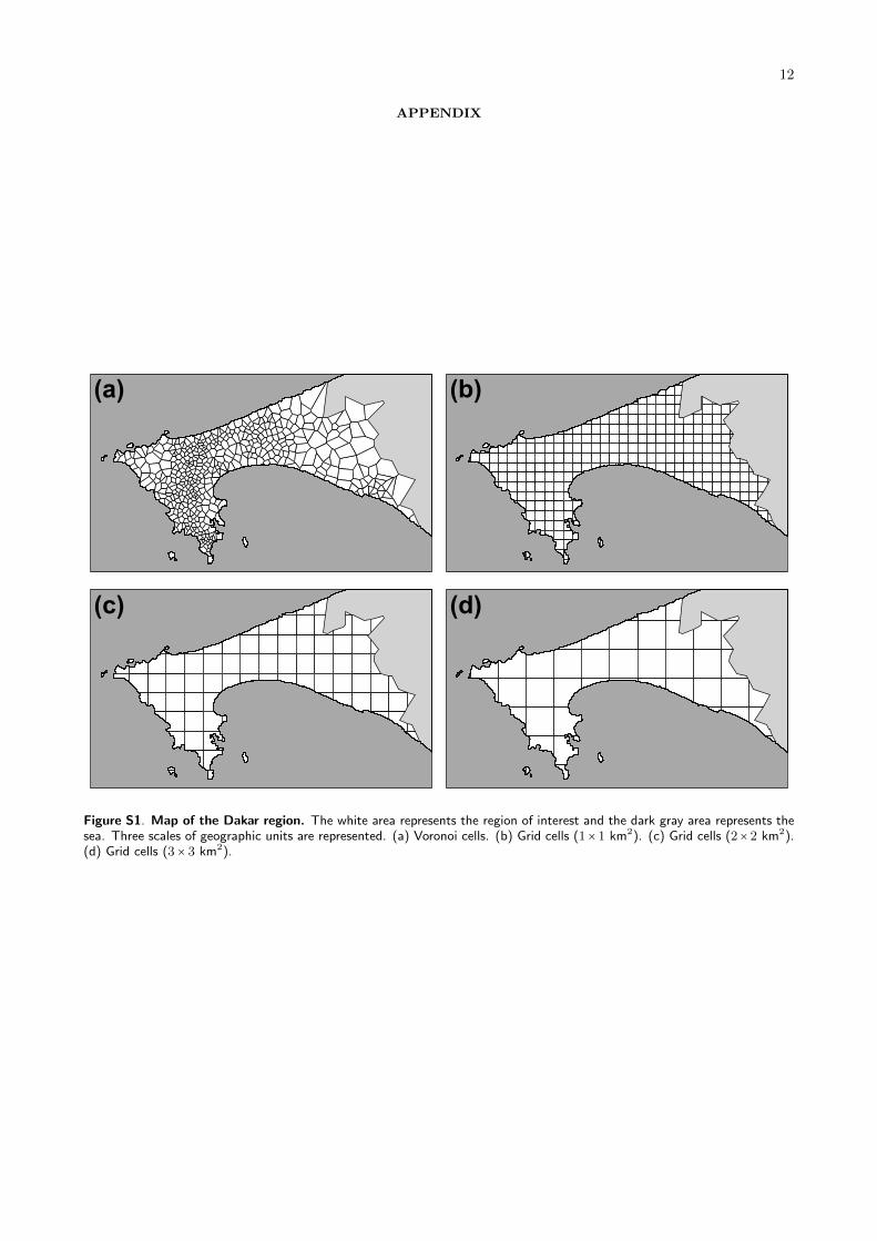
Figure S1. Map of the Dakar region. The white area represents the region of interest and the dark gray area represents thesea. Three scales of geographic units are represented. (a) Voronoi cells. (b) Grid cells (1× 1 km2). (c) Grid cells (2× 2 km2).(d) Grid cells (3 × 3 km2).
13
50 100 150 200 250 300
40
50
60
70
80
90
100
Number of users (x 103)
Tota
l sha
red
surf
ace
area
(%
)(a)
50 100 150 200 250 300
40
50
60
70
80
90
100
Number of users (x 103)
Tota
l sha
red
surf
ace
area
(%
)
(b)
50 100 150 200 250 300
40
50
60
70
80
90
100
Number of users (x 103)
Tota
l sha
red
surf
ace
area
(%
)
(c)
50 100 150 200 250 300
40
50
60
70
80
90
100
Number of users (x 103)
Tota
l sha
red
surf
ace
area
(%
)
(d)
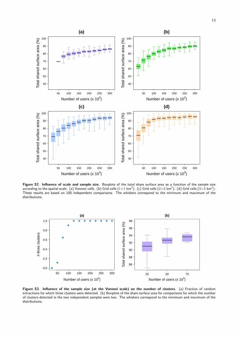
Figure S2. Influence of scale and sample size. Boxplots of the total share surface area as a function of the sample sizeaccording to the spatial scale. (a) Voronoi cells. (b) Grid cells (1×1 km2). (c) Grid cells (2×2 km2). (d) Grid cells (3×3 km2).These results are based on 100 independent comparisons. The whiskers correspond to the minimum and maximum of thedistributions.
50 100 150 200 250 300
0.0
0.2
0.4
0.6
0.8
1.0
Number of users (x 103)
# th
ree
clus
ters
(a)
25 50 75
86
88
90
92
94
96
98
Number of users (x 103)
Tota
l sha
red
surf
ace
area
(%
)
(b)
Figure S3. Influence of the sample size (at the Voronoi scale) on the number of clusters. (a) Fraction of randomextractions for which three clusters were detected. (b) Boxplots of the share surface area for comparisons for which the numberof clusters detected in the two independent samples were two. The whiskers correspond to the minimum and maximum of thedistributions.
14
0.2 0.4 0.6 0.8
0
5
10
15
δh
Num
ber
of u
sers
(x
104 )
Nd = 1
0.2 0.4 0.6 0.8
0
5
10
15
δh
Num
ber
of u
sers
(x
104 )
Nd = 2
Nh ≥ 1Nh ≥ 5Nh ≥ 10Nh ≥ 15Nh ≥ 20
0.2 0.4 0.6 0.8
0
5
10
15
δh
Num
ber
of u
sers
(x
104 )
Nd = 3
0.2 0.4 0.6 0.8
0
5
10
15
δh
Num
ber
of u
sers
(x
104 )
Nd = 4
0.2 0.4 0.6 0.8
0
5
10
15
δh
Num
ber
of u
sers
(x
104 )
Nd = 5
0.2 0.4 0.6 0.8
0
5
10
15
δh
Num
ber
of u
sers
(x
104 )
Nd = 6
0.2 0.4 0.6 0.8
0
5
10
15
δh
Num
ber
of u
sers
(x
104 )
Nd = 7
0.2 0.4 0.6 0.8
0
5
10
15
δh
Num
ber
of u
sers
(x
104 )
Nd = 8
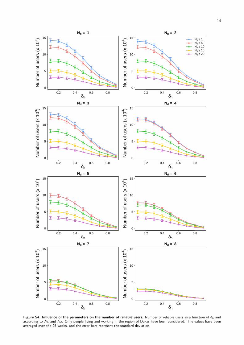
Figure S4. Influence of the parameters on the number of reliable users. Number of reliable users as a function of δh andaccording to Nh and Nd. Only people living and working in the region of Dakar have been considered. The values have beenaveraged over the 25 weeks, and the error bars represent the standard deviation.
15
0.2 0.4 0.6 0.8
0.6
0.7
0.8
0.9
1.0
δh
Fra
ctio
n of
intr
a−zo
nal f
low
s Nd = 1
Nh ≥ 1Nh ≥ 5Nh ≥ 10Nh ≥ 15Nh ≥ 20
0.2 0.4 0.6 0.8
0.6
0.7
0.8
0.9
1.0
δh
Fra
ctio
n of
intr
a−zo
nal f
low
s Nd = 2
0.2 0.4 0.6 0.8
0.6
0.7
0.8
0.9
1.0
δh
Fra
ctio
n of
intr
a−zo
nal f
low
s Nd = 3
0.2 0.4 0.6 0.8
0.6
0.7
0.8
0.9
1.0
δh
Fra
ctio
n of
intr
a−zo
nal f
low
s Nd = 4
0.2 0.4 0.6 0.8
0.6
0.7
0.8
0.9
1.0
δh
Fra
ctio
n of
intr
a−zo
nal f
low
s Nd = 5
0.2 0.4 0.6 0.8
0.6
0.7
0.8
0.9
1.0
δh
Fra
ctio
n of
intr
a−zo
nal f
low
s Nd = 6
0.2 0.4 0.6 0.8
0.6
0.7
0.8
0.9
1.0
δh
Fra
ctio
n of
intr
a−zo
nal f
low
s Nd = 7
0.2 0.4 0.6 0.8
0.6
0.7
0.8
0.9
1.0
δh
Fra
ctio
n of
intr
a−zo
nal f
low
s Nd = 8
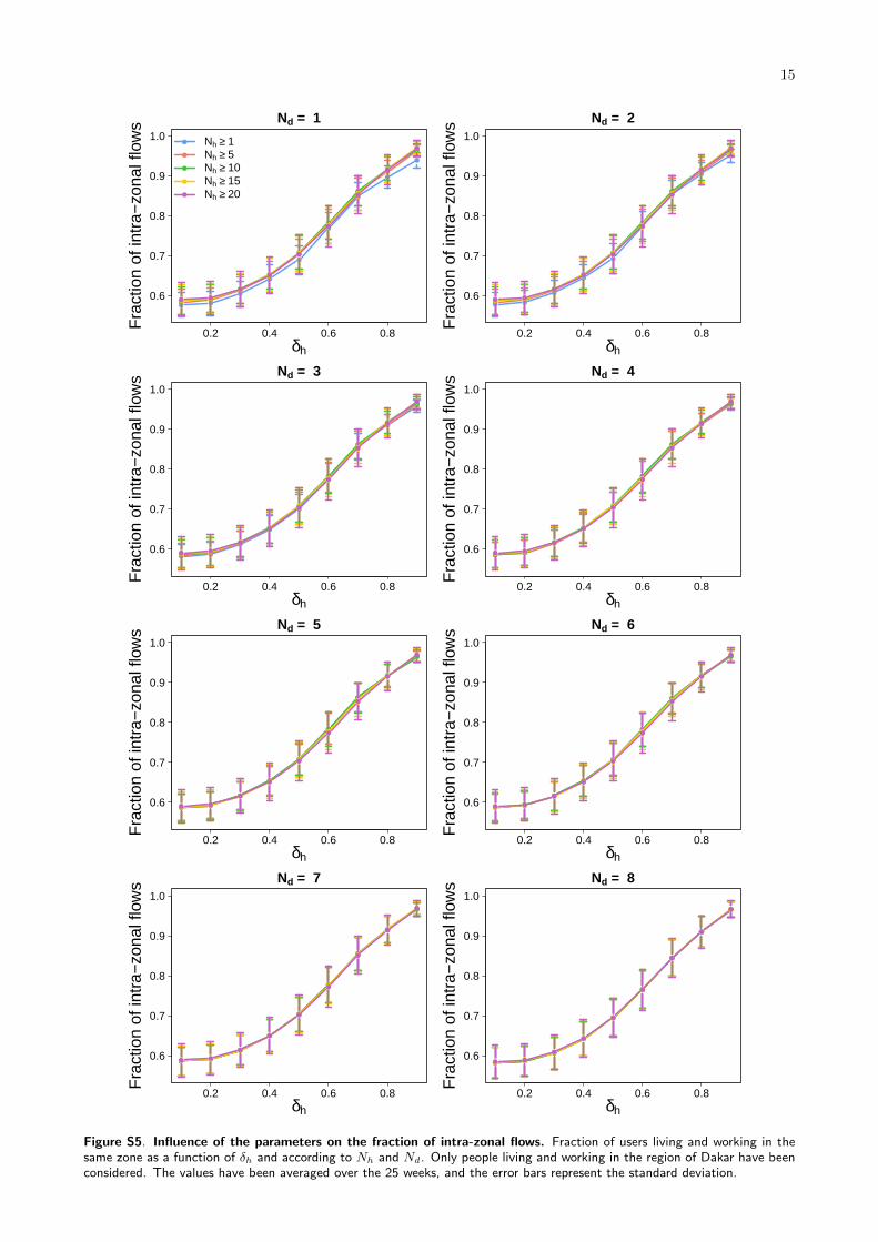
Figure S5. Influence of the parameters on the fraction of intra-zonal flows. Fraction of users living and working in thesame zone as a function of δh and according to Nh and Nd. Only people living and working in the region of Dakar have beenconsidered. The values have been averaged over the 25 weeks, and the error bars represent the standard deviation.

16
5 10 15 20 25
0.85
0.90
0.95
1.00
1.05
1.10
1.15
Nh
#links#links = 11 < #links < 10#links >= 10
Figure S6. Influence of Nh on the number of links. The value have been normalized by the value obtained with Nh = 1.
50 100 150 200 250 300
0.6
0.7
0.8
0.9
1.0
Number of users (x 103)
λ c
VoronoiGrid 1kmGrid 2kmGrid 3km
Figure S7. Influence of scale and sample size. Boxplots of λc as a function of the sample size according to the spatial scale(Voronoi cells and grid cells of 1, 2 and 3 km side length). The distributions are based on 100 independent comparisons withNd = 4, Nh = 12 and δh = 1/3. The whiskers correspond to the minimum and maximum of the distributions.
17
1 2 3 4 5 6 7 8 9 10 11 12
12
11
10
9
8
7
6
5
4
3
2
1
Four weeks period
Fou
r w
eeks
per
iod
(a)
1 2 3 4 5 6 7 8 9 10 11 12
12
11
10
9
8
7
6
5
4
3
2
1
Four weeks periodF
our
wee
ks p
erio
d
(b)
1 2 3 4 5 6 7 8 9 10 11 12
12
11
10
9
8
7
6
5
4
3
2
1
Four weeks period
Fou
r w
eeks
per
iod
(c)
−0.06
−0.04
−0.02
0.00
0.02
λx − λx
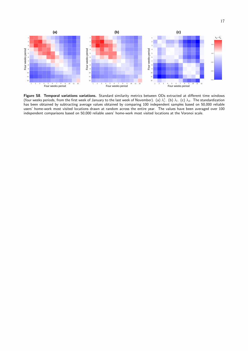
Figure S8. Temporal variations variations. Standard similarity metrics between ODs extracted at different time windows(four weeks periods, from the first week of January to the last week of November). (a) λ∗c . (b) λl. (c) λd. The standardizationhas been obtained by subtracting average values obtained by comparing 100 independent samples based on 50,000 reliableusers’ home-work most visited locations drawn at random across the entire year. The values have been averaged over 100independent comparisons based on 50,000 reliable users’ home-work most visited locations at the Voronoi scale.