ionogram height–time–intensity observations of descending

ARTICLE IN PRESS

1364-6826/$ - se

doi:10.1016/j.ja

�CorrespondE-mail addr

Journal of Atmospheric and Solar-Terrestrial Physics 68 (2006) 539–557

www.elsevier.com/locate/jastp

Ionogram height–time–intensity observations of descendingsporadic E layers at mid-latitude

C. Haldoupisa,�, C. Meekb, N. Christakisc, D. Panchevad, A. Bourdillone

aPhysics Department, University of Crete, Heraklion, 710 03 Crete, GreecebInstitute of Space and Atmospheric Studies, University of Saskatchewan, Canada

cDepartment of Applied Mathematics, University of Crete, GreecedDepartment of Electronics and Electrical Engineering, University of Bath, UK

eIETR/CNRS, Universite de Rennes 1, France

Available online 24 October 2005

Abstract

A new methodology of ionosonde height–time–intensity (HTI) analysis is introduced which allows the investigation of

sporadic E layer (Es) vertical motion and variability. This technique, which is useful in measuring descent rates and tidal

periodicities of Es, is applied on ionogram recordings made during a summer period from solstice to equinox on the island

of Milos (36.71N; 24.51E). On the average, the ionogram HTI analysis revealed a pronounced semidiurnal periodicity in

layer descent and occurrence. It is characterized by a daytime layer starting at 120 km near 06 h local time (LT) and moving

downward to altitudes below 100 km by about 18 h LT when a nighttime layer appears above at �125 km. The latter moves

also downward but at higher descent rates (1.6–2.2 km/h) than the daytime layer (0.8–1.5 km/h). The nighttime Es is

weaker in terms of critical sporadic E frequencies (foEs), has a shorter duration, and tends to occur less during times close

to solstice. Here, a diurnal periodicity in Es becomes dominant. The HTI plots often show the daytime and nighttime Es

connecting with weak traces in the upper E region which occur with a semidiurnal, and at times terdiurnal, periodicity.

These, which are identified as upper E region descending intermediate layers (DIL), play an important role in initiating and

reinforcing the sporadic E layers below 120–125 km. The observations are interpreted by considering the downward

propagation of wind shear convergent nodes that associate with the S2,3 semidiurnal tide in the upper E region and the S1,1

diurnal tide in the lower E region. The daytime sporadic E layer is attributed to the confluence of semidiurnal and diurnal

convergent nodes, which may explain the well-known pre-noon daily maximum observed in foEs. The nighttime layer is

not well understood, although most likely it is associated with the intrusion of the daytime DIL into the lower E region due

to vertical wind shear convergence nodes descending with the semidiurnal tide. It was also found that the descent rates of

sporadic E may not always represent the vertical phase velocities of the tides, especially in the nighttime layers. Finally, the

ionosonde HTI analysis is a promising new tool for exploring long-duration data sets from ionosondes around the globe to

obtain preliminary climatological studies of neutral wind dynamics at E region heights in the lower thermosphere.

r 2005 Elsevier Ltd. All rights reserved.

Keywords: Sporadic E layers; Ionogram HTI plots; Descending layers; Atmospheric tides

e front matter r 2005 Elsevier Ltd. All rights reserved.

stp.2005.03.020

ing author. Tel.: +302810 394222; fax: +30 2810 394201.

ess: [email protected] (C. Haldoupis).

www.elsevier.com/locate/jastp

ARTICLE IN PRESSC. Haldoupis et al. / Journal of Atmospheric and Solar-Terrestrial Physics 68 (2006) 539–557540

1. Introduction

The mid-latitude sporadic E layers (Es), which arethin layers of metallic ion plasma that form at E

region heights between 95 and 125 km, have beenstudied extensively over many years, e.g., seecomprehensive reviews by Whitehead (1989) andMathews (1998). The physics of Es formation isbased on the ‘‘wind shear’’ theory, in which verticalshears in the horizontal neutral wind can cause, bythe combined action of ion-neutral collisionalcoupling and geomagnetic Lorentz forcing, thelong-lived metallic ions to move vertically andconverge into thin and dense plasma layers. Theprocess is governed by ion dynamics, with themagnetized electrons only following the ions tomaintain charge neutrality. In its simplest form,when diffusion and electric field forces are ne-glected, the wind shear theory predicts for thevertical ion drift velocity w at steady state:

w ¼cos I sin I

1þ ðni=oiÞ2

U þðni=oiÞ cos I

1þ ðni=oiÞ2

V . (1)

Here, the notations of Mathews and Bekeny (1979)are used, in which U and V are the geomagneticsouthward and eastward components of the neutralwind (representing approximately the meridionaland zonal wind components, respectively), I is themagnetic dip angle, and ðni=oiÞ ¼ r is the ratio ofion-neutral collision frequency to ion gyrofre-quency. Since the vertical plasma drift becomescollision-dominated below about 125 km wherer2b1, the wind shear mechanism requires for theformation of a layer vertical shears of a properpolarity in the zonal and meridional wind, in accordwith Eq. (1).

Since most Es are situated below about 120 km,they are controlled by vertical zonal wind shearswhich are characterized (for the northern hemi-sphere) by a westward wind above and an eastward,or smaller westward, wind below. Also, Es areknown to descend regularly with time down below100 km where they eventually disappear, apparentlybecause the metallic ion recombination rates be-come increasingly effective. On the other hand, thevertical meridional wind shears, with a northwardwind above and a southward, or smaller northward,wind below, are effective in the upper E region,where they can generate, together with verticalshears in the zonal wind, the so called ‘‘descendingintermediate layers’’ (DILs). These are weak plasmalayers that initiate at the bottom of the F region and

move downward, often merging with the sporadic E

layers below. DILs are considered to be part of thesporadic E layer system because they appear toparticipate in a parenting-like process for Es bysteadily transporting metallic ions down to lower E

region heights (e.g., see Fujitaka and Tohmatsu,1973; Mathews, 1998).

Incoherent scatter radar (ISR) studies and iono-sonde observations show that mid-latitude sporadicE is not as ‘sporadic’ as its name implies but aregularly occurring phenomenon. The repeatabilityin Es layer occurrence and altitude descent areattributed to the global system of the diurnal andsemidiurnal tides in the lower thermosphere. Assummarized by Mathews (1998), the Arecibo ISRobservations revealed a fundamental role played bythe diurnal and semidiurnal tides in the formationand descent of sporadic E layers, which often arealso referred to as ‘‘tidal ion layers’’ (TILs). The 12and 24 h tidal effects on Es formation have beenrecognized also in ionosonde observations, e.g., seeMacDougall (1974), Wilkinson et al. (1992), andSzuszczewicz et al. (1995). The connection betweenEs and tides is not so surprising given that thedominant winds in the E region are the solar tides(Chapman and Lindzen, 1970).

Although there exists an understanding of thetidal variability of descending mid-latitude sporadicE layers, still there are unresolved complexities inthis process which require further study. Forexample, a point of uncertainty relates to the roleand importance of the semidiurnal tides on thedirect formation and descent of Es. Importantquestions also exist with respect to the confluenceof the various tidal modes and what do the descentrates signify. Moreover, there are questions aboutthe tidal effects on basic Es properties, such as thediurnal and seasonal variability of the layers, whichare still not well understood.

The purpose of the present work is to providemore insight into the topic of sporadic E tidalvariability and layer descent by means of using anovel method for the presentation of the ionosondedata. In this method, ionograms are used toconstruct height–time–intensity (HTI) plots forone or more ionosonde frequency bins. Thispresentation, which was developed for the analysisof Canadian advanced digital ionosonde (CADI)data, turned out to be quite suitable for studyingsporadic E layer dynamics and height variability.Also, and in relation to the powerful ISR technique,the HTI methodology can be supplementary

ARTICLE IN PRESSC. Haldoupis et al. / Journal of Atmospheric and Solar-Terrestrial Physics 68 (2006) 539–557 541

because an ionosonde has the advantage of makinglong-term measurements which are necessary forstudying tidal and planetary wave effects on iono-spheric plasma (e.g., see Haldoupis and Pancheva,2002; Pancheva et al., 2003; Haldoupis et al., 2004).

In the following we first introduce the ionosondeHTI method which is applied here on high-timeresolution ionograms. Next, the analysis focuses onfinding the average tidal variations and descent ratesof sporadic E layers during a 3-month periodextending from the summer solstice to equinox.The findings are first presented and then comparedto the Arecibo ISR observations. Then, the physicalpicture that emerges from the present and pastknowledge is presented, followed by a numericalsimulation based on the wind shear theory. Finally,the paper closes with a summary of the main resultsand a few concluding comments.

2. Ionogram height–time–intensity analysis

We introduce a new presentation of the iono-sonde observations which relies on the concept ofrange-time intensity (RTI) plots of a single fre-quency radar. Given that the ionogram represents a‘‘snapshot’’ of the reflected signal power as afunction of (virtual) height and radio frequency,one would select any frequency bin and usesequential ionograms to compute the reflectedpower as a function of height and time, and thusobtain a HTI display. The HTI plot has the meritsof the common RTI radar plot which can monitordynamic changes in the medium. In producing anHTI plot, the choice of the ionosonde frequency isimportant because it relates to the ionosphericelectron density at the reflection height, i.e.,f /

ffiffiffiffiffiffiNe

p. For example, in order to observe daytime

F region changes, a frequency must be selectedwhich is higher than the critical E region frequencyfoE. Also, in order to minimize the height un-certainties, the HTI frequency cannot be near the E

and F layer critical frequencies, otherwise themeasured virtual heights can differ from the realheights significantly.

The software developed for the analysis allowsfirst the selection of several, overlapping or not,ionosonde frequency bins of equal or differentextent, and then computes the corresponding HTIplots within a range of heights versus one 24-h dayby averaging over a given number of days. The 24-htime axis was chosen in order to demonstrate theexistence of tidal periodicities present in the data.

The intensity (power) of the reflected signal is color-(shade-) coded of the averaged power convertedto dB.

Fig. 1 introduces the ionosonde HTI displayswhich were computed from sequential ionograms.These were recorded with a CADI which operatedon the Aegean island of Milos during the summer of1996. Fig. 1 includes four 24-h HTI plots averagedover a period of 6 days, from July 31, 1996 toAugust 05, 1996. The four plots correspond todifferent radio frequency ranges, namely,1.5–3.0MHz (upper left), 3.0–4.0MHz (upper right),4.0–5.0MHz (lower left), and 5.0–7.0MHz (lowerright). As expected, the displays differ because eachdepicts ionospheric changes in electron density atdifferent reflection heights which depend on thesounding frequencies. As seen from the low-frequency (1.5–3.0MHz) HTI plot, the upper iono-sphere is masked during sunlit hours, from about06–18 h local time (LT), because of the build up andzenith angle control of the E region, whereas the riseand fall of the F region bottom-side is well markedduring nighttime. On the other hand, the higherfrequency HTI plots, e.g., see the bottom panels inFig. 1, show considerable temporal structure atupper heights during the entire day, most likelycaused by dynamic processes in the F region.

The most consistent signature in the HTI plots ofFig. 1 are the striations seen below about 130 km.These are attributed to the sporadic E layers. Apronounced semidiurnal periodicity is observed,marked by the two consecutive traces of reflectedpower, one occurring during daytime from about 06to 18 h LT followed by a nighttime trace from about18 to 05 h LT. Both traces start at about 125 km andthen move steadily downward. This downwardsloping of the Es traces portrays the well-knowndescending character of sporadic E. Further inspec-tion shows that the nighttime Es trace is strongerthan the daytime one, causing also images to appearin altitude due to multiple Es-ground reflections.This is at least partly and maybe completely due toreduced ionospheric absrorption at night. Anotherpoint implied from the HTI plots in Fig. 1 is thetransparency of Es, so that upper heights becomealso detectable, a fact which is compatible with thepatchy character of sporadic E (Whitehead, 1989).

Inspection of numerous HTI plots of thetype shown in Fig. 1 suggested that the HTI displayis particularly useful for studying sporadic E

layer dynamics and variability. An advantage deal-ing with sporadic E is that there is very little

ARTICLE IN PRESS

Fig. 1. Typical examples of CADI ionogram HTI plots computed for a 24 h day, averaged over six consecutive days. Each plot

corresponds to a different ionosonde frequency band, marked at the top right corner in each figure. The slopping striations between 100

and 130km are sporadic E layer traces.

C. Haldoupis et al. / Journal of Atmospheric and Solar-Terrestrial Physics 68 (2006) 539–557542

magnetoionic splitting because these are thin layersconfined in altitude in the lower ionosphere. Notealso that for frequencies significantly higher thanfoE there is little, if any, group retardation of theincident radio wave, that is, the echo delays give realheights.

3. Experimental results

The Milos CADI (geographic location 36.71N,24.51E, magnetic latitude 30.81, magnetic dip 52.51,magnetic declination 2.51) operated continuously

from June 23, 1996 to September 30, 1996. It wasprogrammed to perform a 54-s frequency sweep,consisting of 250 steps from 1.5 to 16.0MHz, every5min during daytime and every 2min during night-time from 1900 to 0500 hours universal time (UT)(LT ¼ UT+1.7h). The Milos site was nearly free ofman-made interference, and the measured ionogramswere of good quality. Inspection of the observationsshowed the presence of a fairly continuous and oftenintense Es activity from late June to early September,which makes the present data representative of mid-latitude Es at summertime.


The ionogram HTI analysis was applied for a 24-h daytime base starting at 06 h LT. Because of thevariable nature of Es, HTI plots averaged overseveral sequential days were found to be statisticallymore appropriate in defining long-term trends in thedata. This was shown in Fig. 1, which illustrates aprevailing semidiurnal pattern in occurrence andaltitude descent of sporadic E from July 31 toAugust 5. To appreciate the variability and inter-mittency of Es on a day to day basis, we provide inFig. 2 single day HTI plots from July 31 to August5, which are used to produce the average shown inFig. 1.

The HTI displays in Fig. 2 were computed at thefixed frequency band between 3 and 4MHz, foraltitudes between 90 and 250 km. As seen, thesemidiurnal character of layer formation and heightdescent prevails in nearly all days. Seen are twomain striations of Es reflected power, the daytimeone staring at about 120–125 km near sunrise (06 hLT) and the nighttime one starting at about thesame altitude near sunset (18 h LT). Both traces arenegatively tilted with time due to the downwardtransport of the layers. The reflected signal candisappear and reappear but, it is interesting to note,that this ‘‘on–off’’ sequence occurs mostly along thelayer’s descent trace, which is defined better inthe averaged HTI plots of Fig. 1. Also in most of theplots in Fig. 2, the start of the Es striations connectto upper E region through weak reflection traceswhich also descend with time but at much higherrates, estimated to be in the range of 5–8 km/h.These identify with the well-known intermediatelayers which, according to several Arecibo ISRstudies (e.g., see review of Mathews, 1998), have astrong semidiurnal character, forming two times aday at the bottom of the F region and movingdownward.

Although at times the intermediate layers can alsobe traced in the HTI plots, in most instances theyare not, because they are weak, having low criticalfrequencies below the lowest ionosonde frequencyof 1.5MHz. Also one has to be aware that at theselow-ionosonde frequencies propagation effects aremore significant. Therefore, the estimated heightscan be affected more by group retardation and thuscan be incorrect relative to the real heights. Despitethese limitations however, the present HTI plots canprovide some information on the descending inter-mediate layers as well, which agrees also withprevious ionosonde studies, e.g., see Wilkinsonet al. (1992).

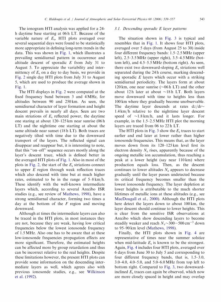
3.1. Descending sporadic E layer patterns

The situation shown in Fig. 3 is typical andresembles that in Fig. 1. It shows four HTI plots,averaged over 5 days (from August 25 to 30) insidefour different frequency bands: 1.5–2.5MHz (upperleft), 2.5–3.5MHz (upper right), 3.5–4.5MHz (bot-tom left), and 4.5–5.5MHz (bottom right). As seen,there exist two downward-sloping Es striations wellseparated during the 24 h course, marking descend-ing sporadic E layers which occur with a strikingsemidiurnal periodicity. The layers form at about120 km, one near sunrise (�06 h LT) and the otherabout 12 h later at about �18 h LT. Both layersmove downward with time to heights less than100 km where they gradually become unobservable.The daytime layer descends at rates dz=dt�

1:4 km=h relative to the nighttime layer descentspeed of �1.8 km/h, and it lasts longer. Forexample, in the 1.5–2.5MHz HTI plot the morninglayers are traced from 06 to 22 h LT.

The HTI plots in Fig. 3 show the Es traces to startearlier and end later at lower rather than higherionosonde frequencies. This means that, as the layermoves down from its 120–125 km level first itselectron density Ne rises, apparently because of theongoing metallic ion accumulation, thus reaching apeak at a lower height (say near 110 km) whereproduction equals loss. Then, as the descentcontinues to lower altitudes Ne appears to decreasegradually until the layer passes undetected becauseits critical frequency becomes smaller than thelowest ionosonde frequency. The layer depletion atlower heights is attributable to the much shorterlifetimes of metallic ions at these altitudes (e.g., seeMacDougall et al., 2000). Although the HTI plotshere detect the layers down to about 100 km, thelayer descent should continue to lower heights. Thisis clear from the sensitive ISR observations atArecibo which show descending layers to becomesteadily weaker and reach Ne�3002500 cm�3 downto 95–90 km level (Mathews, 1998).

Finally, the HTI plots shown in Fig. 4 arerepresentative of times near the summer solsticewhen mid-latitude Es is known to be the strongest.Again, Fig. 4 includes four HTI plots, averaged over6 days from June 30 to July 5 and corresponding tofour different frequency bands, that is, 1.5–3.0,3.0–4.0, 4.0–5.0, and 5.0–6.0MHz from top left tobottom right. Compared to Fig. 3, two downward-inclined Es traces can again be observed, which noware more closely spaced in height and may overlap

ARTICLE IN PRESS

Fig. 2. HTI plots for each of the 6 days used to compute the averaged HTI displays shown in Fig. 1. All plots are computed for the

ionosonde frequency band between 3 and 4MHz, and for altitudes between 100 and 250 km. The 24 h time axis is in LT starting at 06 h.

Despite the variability and intermittency from day to day, there is a regular pattern seen in sporadic E layer occurrence and altitude

descent which is dominated by a semidiurnal periodicity. Also seen is a close relation to the upper E region descending intermediate layers.


ARTICLE IN PRESS

Fig. 3. Milos CADI HTI plots averaged over 6 days from August 25–30, 1996. The descending sporadic E layers appear with a striking

semidiurnal periodicity. As seen, a daytime layer starts near 120 km at about 06 h LT, followed by a nighttime layer 12 h later. Both layers

move downward with descent rates near 1.4 and 1.8 km/h, respectively.

C. Haldoupis et al. / Journal of Atmospheric and Solar-Terrestrial Physics 68 (2006) 539–557 545

in time for many hours during the day. The firsttrace starts near 125 km at about 05 h LT, whereasthe second becomes detectable near 130 km at about10–11 h LT. Both these HTI striations are tilteddownward with time, having slopes ranging between0.8 and 1.1 km/h. Contrary to the cases presented inFigs. 1 and 3, the situation in Fig. 4 indicates amuch weaker semidiurnal effect.

3.2. Sporadic E layer descending trends during

summer

As mentioned, the CADI observations coveredthe interval from June 23 to September 20, 1996.Detailed HTI analysis suggested some systematicdifferences in the descent of sporadic E layers astime progresses from solstice to equinox. In this

ARTICLE IN PRESS

Fig. 4. Same as Fig. 3 but for a time interval near the summer solstice. See text for more details.


section we summarize the average trends in layerdescent which may be of significance for the diurnaland seasonal sporadic E variability. We recognize,however, that the general validity of these resultscannot be established from a single summer analysisand that ionogram data from more summers need tobe studied.

Fig. 5 shows three HTI plots covering theobservations from June 23 to the end of July,1996. All plots were computed for ionosondefrequencies between 4.0 and 7.0MHz which arehigher than the anticipated E region critical

frequencies foE. Thus, the measured (virtual) Es

heights are near to the real ones.The upper and middle panel in Fig. 5, which

correspond to the last week of June and the first 3weeks of July, respectively, show a dominantdiurnal periodicity in Es layer descent. A layer firstappears at about 115 km near 05 h LT and then isseen to move slowly down toward 100 km for morethan 12 h until it becomes undetectable. This trace,which is attributed to a convergence node of thediurnal tide, is followed by a second one thatappears during the day at about 120 km undergoing

ARTICLE IN PRESS

Fig. 5. Averaged HTI plots representing sporadic E layer descent and variability for times near summer solstice (from June 23 to July 31).



a slow downward motion through the entire nightand into the morning sector. This is consideredagain to be due to a subsequent convergence nodeof the diurnal tide. Note that the vertical (altitude)separation of the two layers is close to about 20 km,and represents here the vertical wavelength of thediurnal tide.

A weak semidiurnal effect is seen clearly in theupper panel of Fig. 5 (during June 23–30) but this isobscured in the middle panel, although it is alsopresent there as well at least for part of the timeinterval under consideration (e.g., see also the HTIplots in Fig. 3 which correspond to the interval fromJune 30 to July 5). Finally, the HTI plot at thebottom of Fig. 5 corresponds to the last week ofJuly. It shows the HTI plot to be dominated bythree sloping Es traces, distributed more or lessevenly during the 24-h day, which are attributed tothe effects of a terdiurnal tide. The presence of astrong terdiurnal periodicity in the same Milos dataduring the last days of July has been first recognizedand reported in a separate study by Haldoupis et al.(2004).

Estimates of descent rates in the interval fromJune 23 to July 31 take values between 0.8 and1.3 km/h, with an average near 1.0 km/h. If weassume that on average the layers descend with thephase velocity of the diurnal tide, then thiscorresponds to a vertical wavelength of about25 km, which is close to the theoretical wavelengthof 28 km of the S1,1 diurnal tidal mode (Forbes,1984).

Fig. 6 shows the situation prevailing for the restof the Milos CADI data, from August 1 toSeptember 20, when sporadic E is known to becomegradually weaker with time, past the summersolstice (Whitehead, 1989). The upper and middlepanel in Fig. 6 are HTI averages for the periodsfrom August 1 to 15 and from August 16 to 31,respectively, whereas the bottom panel refers to theentire month of September. As seen, there is asemidiurnal periodicity present in all HTI plotswhich is more pronounced in the lower two panels.On average, we observe two well separated andnegatively sloping traces which correspond to adaytime and a nighttime sporadic E that formaround 120 km at about 06 and 17 h LT, respec-tively, and descend to lower heights with time, asdiscussed also in Figs. 1 and 3. The descent rateswere found to be 1.470.2 and 1.970.3 km/h, forthe daytime and nighttime layers, respectively.These values are consistently larger than the descent

rates measured earlier in the summer during the firstweeks of July.

3.3. Periodicities in foEs

The HTI plots show a weak semidiurnal patternin Es layer descent during June–July which becomesstronger in the late summer during August–Septem-ber. This is also supported from the analysis of thecorresponding Es critical frequency, foEs, timeseries. Note that foEs is expressed in MHz andused widely to quantify the sporadic E layervariability. In a recent paper by Haldoupis et al.(2004), the Milos CADI foEs data were used tostudy the tidal and planetary wave periodicities insporadic E electron densities. It was shown that,besides the leading roles of the diurnal andsemidiurnal tides in Es formation and strength,there is often also a weaker but significantcontribution from the terdiurnal tide. This isconfirmed also here by the HTI analysis, as seenfor example at the bottom plot of Fig. 5. Note that,Haldoupis et al. (2004) have shown that both thesemidiurnal and terdiurnal spectral peaks are real 12and 8 h periodicities and not harmonics of adistorted diurnal oscillation.

Fig. 7 summarizes the Milos foEs measurementsfrom June 27 to July 21, when the diurnal tidalcontrol of Es layer descent is clearly present in theHTI plots. The foEs time sequence is made of 10-min samples and is plotted in the top panel whereasits amplitude spectrum is plotted below. As seen,both the foEs time series and spectrum aredominated by a strong peak at 24-h, whereas muchweaker peaks in the spectrum exist at 12 and 8 h,suggesting also a role for the semidiurnal andterdiurnal tides. Finally the bottom plot in Fig. 7shows the mean diurnal variation of foEs averagedover the June–July time interval under considera-tion. This is dominated by a main peak whichsuggests a dominant diurnal periodicity. This peakoccurs prior to local noon near 10 h LT, a fact thathas been well known for many years, although it isstill not well understood (Whitehead, 1989). Aweaker peak is also seen near 18 h LT, about 8 hapart from the strong peak near 10 h LT, causedmost likely by the action of the terdiurnal tide whichwas also present in the data. Note that in the lastplot there is no clear evidence for a semidiurnalperiodicity.

Finally, Fig. 8 is the same as Fig. 7, but it refers tothe August 01–31 period when there is a clear

ARTICLE IN PRESS

Fig. 6. Same as in Fig. 5, but for later in the summer, from August 1 to September 21. During these times the observed semidiurnal

periodicity intensifies and dominates the layer descent and diurnal variability.


semidiurnal control on the layer formation anddescent. This 12-h periodicity revealed by the HTIplots is also embedded in foEs as well, as shown inthe corresponding amplitude spectrum plotted in

the middle panel of Fig. 8. As seen, there is a 12-hpeak that is equally strong as the 24-h (diurnal)periodicity, in contrast with the situation in Fig. 7.Furthermore, the mean diurnal variation during

ARTICLE IN PRESS

Milos CADI 27 June - 21 July 1996

0 2 4 6 8 10 12 14 16 18 20 22 24Day Number (27June - 21July1996)

0

2

4

6

8

10

12

14

foE

s (M

Hz)

foEs (10-min data), Milos

6 8 10 12 14 16 18 20 22 24 26 28 30

LT

2

3

4

5

6

7

foE

s (M

Hz)

foEs, Milos24 June-21 July, 1996

hourly data

10-min data

4 8 12 16 20 24 28 32 36Period (hours)

0.0

0.2

0.4

0.6

0.8

1.0

1.2

Am

plit

ude

Spe

ctru

m (

MH

z)

95%

foEs, Milos27 June-21 July, 1996

Fig. 7. Critical sporadic E frequency (foEs) analysis for the period from June 27 to July 21, near summer solstice. The upper panel is the

hourly means time series, the middle panel is the corresponding amplitude spectrum, and the bottom plot shows the mean daily variation

starting at 06 h LT. The diurnal periodicity dominates.


August, which is presented in the bottom panel,shows a well-defined secondary peak in foEs around22 h LT, about 12 h away from the strongest peaknear 10 h LT. It is interesting to note that similarresults (not shown here) were also obtained byanalyzing Rome ionosonde data for the same timeintervals of 27 June–21 July and 01–31 August,1996.

4. Comparison with ISR observations

As summarized in the review paper by Mathews(1998), the regular occurrence as well as the verticalmotion and variability of mid-latitude sporadic E

are shaped by the semidiurnal and diurnal tidesin the lower thermosphere. The tides can pro-vide downward propagating wind shears of ion

ARTICLE IN PRESS

Milos CADI . August 01 - 31 1996

0 2 4 6 8 10 12 14 16 18 20 22 24 26 28 30Day Number (1 - 31August 1996)

2

4

6

8

10

12

14

foE

s (M

Hz)

foEs (10-min data), Milos

4 8 12 16 20 24 28 32 36

Period (hours)

0.0

0.2

0.4

0.6

0.8

1.0

1.2

Am

plit

ude

Spe

ctru

m (

MH

z)

95%

foEs, MilosAugust, 1996

6 8 10 12 14 16 18 20 22 24 26 28 30

LT

2

3

4

5

6

7

foE

s (M

Hz)

foEs, MilosAugust, 1996

hourly data

10-min data

Fig. 8. Same as Fig. 7, but for the month of August, showing the presence of a strong semidiurnal periodicity in foEs, in line also with the

HTI plots in Fig. 6.


convergent nodes, which can account for theformation and vertical transport of the layers, aswas shown theoretically by Axford (1963), numeri-cally by Chimonas and Axford (1968), and experi-mentally by Mathews and Bekeny (1979) usingArecibo ISR observations.

The Arecibo ISR studies revealed a regularsemidiurnal pattern for the descending intermediatelayers in the upper E region, a dominant diurnalperiodicity for the lower E region sporadic layers,

and a confluence zone between about 120 and100 km where both tidal modes can be active. Tonget al. (1988) presented continuous layer motionsobtained from Arecibo height–time layer trajec-tories observed during January 3–6, 1981 andNovember 8–10, 1985. Inspection of these plotsshow: (1) A once-per-day periodicity for the day-time sporadic E layers forming near 115 km atabout 0600 h LT and descending down to 90 kmwith a speed of about 1.1 km/h. (2) A twice-per-day


periodicity for the intermediate layers at upperheights that move fast down to 120 km with speedsranging between 5 and 8 km/h, while at times thesituation can be complicated by the additionalaction of a quarterdiurnal tide in the upper E

region. (3) Although not emphasized in the Tonget al. (1988) paper, the plots show also an once-per-day weaker Es trajectory caused by nighttimesporadic E layers forming near 120 km at about1600–1800 h LT and moving downward with speedsnear 2.0 km/h.

In comparing the ionosonde and ISR observa-tions, one should bear in mind that the ionosonde ismuch less sensitive because it needs electrondensities Ne larger than �5� 104 cm�3 in order forits signal to be totally reflected. This means thationosonde Es layer returns are biased to altitudesbetween about 100 and 120 km where the layers arestrongest. As for the intermediate layers above130 km usually these go unnoticed by the ionosondebecause they are not dense enough to cause totalreflections and/or because of blanketing effects fromthe strong layers below. On the other hand, theArecibo results are based on a few limited observa-tional periods mostly during winter, whereas theCADI HTI results cover the entire period from thesummer solstice to equinox.

Despite the sensitivity limitations, the presentionosonde results are in reasonable agreement withseveral of the ISR characteristics of sporadic E layerdescent and occurrence. Namely, the HTI plotsshow the presence of daytime and nighttime Es

layers that form near 120 km around 0600 and1800 h LT, respectively, which then descend steadilywith height at rates dz/dt that are comparable withISR estimates. Also, the faint HTI traces seen attimes well above 130 km occur mostly with asemidiurnal periodicity and have descent rates dz/

dt between 5 and 8 km/h, which again compare wellwith the Arecibo observations of intermediatelayers. On the other hand, there are also differencesbetween the ionosonde and ISR findings. Forexample, the ionogram HTI plots show, in line withprevious ionosonde studies (e.g., see MacDougall,1974; Wilkinson et al., 1992; Szuszczewicz et al.,1995), that the twice-per-day periodicity in Es layerdescent and occurrence is much more pronouncedthan the prevailing diurnal periodicity seen in theArecibo Es observations (Mathews, 1998). More-over, the current data suggest a terdiurnal periodi-city being often present during summer, a fact thathas not been identified so far with the Arecibo ISR.

These discrepancies however might be expectedbecause long-term Arecibo observations of sporadicE are limited and the existing ones may not berepresentative of the average summer conditionsdealt with in this ionosonde study.

5. The physical picture

As Mathews (1998) points out in his reviewpaper, the prevailing periodicities in mid-latitudesporadic E result from the confluence of the verticaltidal wind shears in the lower thermosphere,particularly in the altitude range between 100 and120 km. The observed diurnal, semidiurnal andterdiurnal periodicities, seen in the occurrence,altitude descent and strength (foEs) of sporadic E,show the decisive role played by the atmospherictides which provide the convergent wind shearsneeded for the layers to form and build up, whiletidal phase progression downward causes theiraltitude descent. Next, we rely on present and pastevidence to interpret our main results as follows.

We start with the pronounced semidiurnalperiodicity in Es, manifested in the ionosonde HTIplots by a daytime and a nighttime descending layer.This can be attributed to the semidiurnal characterof the DIL which act as suppliers of metallic ions forthe lower E region. DIL form in the upper E regioninside a convergent node in the vertical wind profileassociated with a downward propagating semidiur-nal tide. According to wind shear theory, a layerremains at the shear convergence null only if itforms fast compared with the time required for thenull to propagate downward a distance equal to thelayer’s width (e.g., see Chimonas and Axford, 1968).In the upper E region, the layers form rapidlybecause the ion–neutral collision frequency is small,therefore they tend to ‘‘stick’’ at the wind shearconvergence null as this moves down with the tidalvertical phase velocity.

At heights below about 125–120 km the situationchanges because ion–neutral collisions becomeincreasingly effective. There, the downward trans-port of intermediate layers slows down becausevertical ion convergence becomes slower, thus thelayers cannot form fast enough in order to remaininside the tidal convergence null as in the upper E

region. In effect, the layers lag steadily behind thetidal convergence null, thus descending at ratesincreasingly smaller than the vertical phase velocityof the tide. This slow descent continues until thefollowing divergent node catches up with the layer,


to impose small layer uplifts and some verticalplasma divergence that may disrupt and disperse thelayer. Finally, and depending upon the amplitudeand phase velocity of the semidiurnal tide, there is alower altitude at which the ion–neutral collisionfrequency is high enough, so that it does not allowthe 12-h tide to have any effect on the layer.

In line also with the Arecibo ISR observations(e.g., see Tong et al., 1988), the morning Es layer,which starts at about 120 km near 06 h LT andmoves steadily down to 100 km by the evening, isattributed mainly, but not fully, to the diurnal S1,1

tide which is known to dominate in the lower E

region, e.g., see Harper (1977). On the other hand,the semidiurnal tide must also contribute in themorning Es formation as well. This is supported bythe fact that often the morning sporadic E layer isborn out of a DIL reaching 125 km at about 06 hLT. By assuming the 12 and 24-h tidal convergencenodes to be approximately in phase, their actioncombines in the morning hours to reinforce Es. Thisprocess may lead to the well-known pre-noonmaximum in Es layer occurrence and strength near110 km at about 1000 h LT, as manifested by thelayer’s critical frequency Es daily peak (Whitehead,1989).

As time progresses, the semidiurnal tidal effect onthe daytime layer ceases because the 12-h conver-gence null moves fast downward at phase speedsbetween 5 and 8 km/h so it leaves the layer behind.On the other hand, the daytime layer can respond tothe 24-h tidal forcing and can be transported downwith the vertical phase velocity of the diurnal tidewhich is considerably smaller than that of thesemidiurnal tide. The observed mean descent speedsfor the morning layers range from 0.8 to 1.6 km/h,which compare well with the vertical phase velo-cities of the diurnal tides having wavelengthsbetween 20 and 40 km, respectively.

The nighttime sporadic E layer which appears atabout 1800 UT near 125 km, is weaker, has shorterduration, and descends faster relative to the daytimelayer. Since it cannot be associated with the diurnaltide, it is interpreted as being due to the intrusionand intensification of the daytime DIL into thelower E region under the action of a vertical windshear associated with the semidiurnal tidal windprofile. The observed descent rates between 1.7 and2.2 km/h for the nighttime Es can be explained asthe result of increased collisions which slow thelayer descent relative to the phase velocity of thetide. The faster descent rates for the evening layer

and its reduced layer strength and duration relativeto the daytime layer, are properties which favor thesemidiurnal tide as the main driver during nighttimehours.

The diminished semidiurnal periodicity seenduring several days of observations, especiallyduring periods near solstice, can be understood asthe result of weakening of the semidiurnal tidalactivity in the upper E region. In the same way, theterdiurnal periodicities seen occasionally can beinterpreted as being due to enhanced terdiurnal tidalaction in the upper E region and their mixture withthe diurnal and semidiurnal tides inside the sporadicE confluence zone between 100 and 130 km.

6. Numerical simulation

In order to substantiate the interpretation above,we performed a numerical simulation of intermedi-ate and sporadic E layer vertical trajectories byusing the methodology introduced first by Chimo-nas and Axford (1968). In modeling the layervertical motions, we solve numerically Eq. (1),which is a first-order ordinary differential equation,dz=dt ¼ wðz; tÞ, by using a varying time-step fourth-order Runge–Kutta algorithm with a maximumallowed time-step of 10 s. In solving Eq. (1) we usean oversimplified wind system that is dominated bya semidiurnal tide in the upper E region and adiurnal tide at lower E region, in line with existingArecibo observations (e.g., see Harper 1977) and theEs modeling methodology of Mathews and Bekeny(1979). For clarity, the numerical results wereobtained by using only a zonal horizontal windcomponent, thus meridional wind U was set to zeroin Eq. (1), while the zonal wind profile V was setequal to

V ¼ V0 expz� z0

2H

� �cos

2plz

ðz� z0Þ þ2pTðt� t0Þ

� �,

(2)

for both the 24- and 12-h tidal winds which wereadded to get the total wind system.

In the last equation, T and lz are the period andvertical wavelength of the tidal wind, H is arepresentative scale height for the lower thermo-sphere between 80 and 200 km, z0 is a lower altitudeboundary set equal to either 85 km for diurnal, or95 km for semidiurnal tides, and t0 is the phase ofthe tide at the representative scale height. Theion–neutral collision frequency profile between 80


and 200 km was based on a least-squares fit of the ni/oi altitude data used by Bishop and Earle (2003) asbeing more appropriate for metallic ion plasma inthe lower mesosphere. With respect to the tidalparameters, these were kept similar to the ones usedby Tong et al. (1988) for the diurnal (semidiurnal)tide: T ¼ 24 h (12 h), lz ¼ 25 km (90 km), V0 ¼

20m=s (3m/s), z0 ¼ 85 km (95 km), t0 ¼ 9 h (5 h),H ¼ 5:5 km (5.5 km). Based on the tidal wave-lengths, the downward phase velocities for thediurnal and semidiurnal tide were near 1.1 and7.5 km/h, respectively.

Typical numerical results for the tidal ion layertrajectories are grouped in Fig. 9. The solid anddashed lines correspond to altitude versus timetrajectories of metallic ion layers that form within aconvergent node of a vertical wind shear in thediurnal and semidiurnal sinusoidal wind profiles,respectively. The shear convergent nodes werelaunched at about 120 km for the diurnal and200 km for the semidiurnal tide, and this patternwas repeated every 24 and 12 h, respectively. Thetime axis in Fig. 9 starts at 06 h LT, in order forthese results to compare with the ionosonde HTIobservations presented earlier.

As expected by the wind shear theory, the netdownward layer transport follows the phase velocity

80

100

120

140

160

200

06:00 12:00 18:00 24:00 06

Local T

180

Alt

itu

de

(km

)

Fig. 9. Numerical simulation results based on basic wind shear theory p

S2,3 semidiurnal tide in the upper E region and a S1,1 diurnal tide in the l

metallic ion layer trajectories that form inside convergent nodes of vert

vertical phase velocities of the tides. The inclined bars represent the ant

purposes. See text for more details.

of the tidal convergent node at higher altitudeswhere slopes are straight lines. This applies down toa level where the enhanced ion–neutral collisions actto slow down the layer’s descent until this reaches astagnation altitude or ‘‘dumping level’’, a term firstintroduced by Chimonas and Axford (1968). There,and only in principle, the layer can oscillate slightlyin height with the tidal period under the forcing ofconsecutive convergent and divergent wind shearnodes as they move downward across the layer’sdumping level. Given that the shear horizontal windpolarity is fixed, the model shows that the layerstagnation level depends primarily on the verticaltidal wavelength, or its phase velocity, and secon-darily on the tidal wind amplitude.

For the adopted tidal parameters given earlier,Fig. 9 shows that the 1.04 km/h downward phasespeed of the 24-h tide is slow enough to bring an ionlayer along a convergent node down to about 95 kmwhere it starts slowing down and reaches stagnationat about 85 km. For the upper E region semidiurnaltide, which has a vertical wavelength of 90 km (nearto that of a S2,3 tide) and thus a downward-phasevelocity of 7.5 km/h, the downward-moving layertrajectory starts departing from a straight line atabout 135 km in order to reach gradually itsstagnation level at about 105 km.

:00 06:0012:00 18:00 24:00

ime (hrs)

redictions and a oversimplified tidal wind system dominated by a

ower E region. The curves shown (solid and dashed) correspond to

ical wind shears in the tidal wind which move downward with the

icipated traces of sporadic E, and they are sketched in for clarity


The shaded, downward tilted, bars in the lowerpart of Fig. 9, which are sketched in to be parallel tothe predicted ion trajectories, depict the alternatingdaytime and nighttime sporadic E layer traces whichare expected to form between 100 and 120 km. Asseen, for the descending daytime sporadic E layerthere is an interval of several hours, from about 06to 14 h LT, where there exists a confluence of the 24-and 12-h tides between about 120 and 105 km.There, the descending intermediate layer, which isbrought down from the upper E region by thesemidiurnal tide (dashed lines), is transferred fullyinto the slowly descending convergent node of thediurnal tide (solid lines). It is interesting to note thatthis is the time interval when the strongest E layersare observed, with critical frequencies foEs reachingtheir daily peak near 10 h LT.

As for the evening and night hours, when thenighttime Es layer forms, Fig. 9 shows no confluencebetween the 12- and 24-h tidal convergent nodesbecause they are well separated in height, thus theEs layer forming process is controlled only by thesemidiurnal tide. This tide transports the daytimeDIL down into the lower E region where its descentis slowed down considerably by collisions relative tothe phase velocity of the tidal convergent node.According to Fig. 9, the daytime intermediate layercan form the core of the nighttime sporadic E

which, as the observations show, is weaker, it hasshorter duration, and reaches bottom heights not aslow as the morning (or daytime) layer. These modelinferences are in good agreement with the ISRobservations of nighttime sporadic E shown in Tonget al. (1988).

It is also interesting to note that the shaded barsalong the layer trajectories, which act as sporadic E

tracers, have slopes near 1.1 km/h and 1.8 km/h forthe daytime and nighttime sectors respectively,which are in fair agreement with the measuredHTI descent rates. It is important to clarify furtherthat the nighttime layer descent rates can be muchsmaller than the phase velocity of the drivingsemidiurnal tide, thus one needs to be cautiouswhen using them to compute the vertical tidalwavelength. On the other hand, the descent rates ofthe morning layer estimated from the HTI iono-sonde plots are indeed close to the phase velocity ofthe diurnal tide.

In summary, the results of this simplified simula-tion are close to the main observational factsobtained with HTI analysis, e.g., compare thesimilarity between Figs. 9 and 4. We conclude, that

although the present modeling results rely on thevery basic wind shear theory and oversimplifiedassumptions about the wind system, they support atleast some aspects of the physical picture andunderstanding discussed in the previous section.

7. Summary and concluding comments

The main findings of the ionogram HTI analysisof the Milos CADI sporadic E measurements aresummarized as follows:

1.
The HTI ionogram analysis revealed a semidiur-nal periodicity in the formation and altitudedescent of sporadic E which dominates mostsummertime observations. A daytime layer formsat about 120 km near sunrise and descendssteadily downward below 100 km by 18 h LT.At about this time a nighttime layer appearsabove at �125 km which also moves downwardat a somewhat larger descent rate than thedaytime layer. From about 16–22 h LT it ispossible at times to observe both layers, that is,the daytime below and nighttime above, coexist-ing.
2.
For the summertime observations under consid-eration, there were time intervals close to solsticewhen the observed semidiurnal periodicity insporadic E layer descent and occurrence is weakand a diurnal periodicity becomes predominant.During those times the layers descend at a slowerrate near 1.0 km/h. On the other hand, thesemidiurnal periodicity prevails clearly afterabout the end of July as we move towardequinox when Es becomes gradually weaker.During these times the layers descend faster withrates dz/dt near 1.5 km/h for the daytime layerand 1.9 km/h for the nighttime one.
3.
As the sporadic E layers descend with altitudethey may disappear and reappear abruptly,sometimes in a periodic-like fashion, but on theaverage always tend to re-occur near and aboutthe mean slope of altitude descend. In theirdownward motion, the layers first strengthen interms of electron density down to about 110 kmand then weaken gradually till they becomeunobservable below about 100 km. This isparticularly true for the daytime layer.
4.
The HTI analysis reveals at times weak iono-sonde traces in the upper E region, that is, atheights above 125–130 km. These upper E regionlayers appear to occur with a strong semidiurnal,


and at times terdiurnal, periodicity while theydescend much faster at rates dz/dt ranging fromabout 5 to 8 km/h. Also, they appear to connectwith, and possibly initiate and/or reinforce, thesporadic E layers that form below 120–125 km.

The key findings of the HTI analysis wereinterpreted with the aid of using basic wind sheartheory and taking into account the forcing effects ofthe semidiurnal and diurnal tides in the lowerthermosphere by assuming an oversimplified windsystem. The role of tides is crucial because theyprovide downward propagating wind shears of ionconvergent nodes that form and transport the layersto lower heights. Our study shows that thesemidiurnal tide, which dominates over the diurnaltide in the upper E region, plays an important rolenot only in the formation and transport of thedescending intermediate layers but also on the lowerE region sporadic E layers, especially duringevening and nighttime hours.

We need to stress that the physical picturediscussed in this paper is certainly simplified becauseother factors, which may affect the sporadic E layerformation, were downplayed or ignored. Forexample, electric field and plasma diffusion effectswere not considered as this is a common practice indealing with mid-latitude sporadic E. Also verticalwind shears in the meridional tidal winds wereignored because at altitudes below 120 km they havea minimal effect; on the other hand, the verticalshears in the zonal wind can be quite effective notonly at lower heights but in the upper E region aswell. No mention was made of gravity wave effects,which can be important at times in reinforcing ordisrupting the tidal forcing of the layers. The mostserious omission however has to do with themechanisms of transport, production and loss ofmetallic ions, for which there is very little knowledgeavailable. Certainly, the metallic ion lifetimesshould be important for obtaining a more thoroughunderstanding of the ionosonde data. For example,the weakening of the layers as they move downbelow about 110 km should be affected seriously bythe anticipated decrease of metallic ion lifetimeswith decreasing altitude.

Finally, we have introduced in this paper a newtechnique for analyzing the ionogram recordingswhich can help obtain new physical insight into thecomplex processes of interaction between atmo-spheric wave dynamics and the ionospheric plasma,particularly with respect to the physics of the

plasma-layering phenomena in the upper and lowerE region. Although the present HTI ionogramanalysis was based on a limited data base, it offeredsome new hints as how to solve long standingproblems on mid-latitude sporadic E, such as, themystery of the seasonal sporadic E layer morphol-ogy that shows a pronounced maximum in thesummer and a small maximum in winter. It is hopedto take up this problem in a future study.

Acknowledgments

This work was made possible with the support of:(a) the European Office of Aerospace Research andDevelopment (EOARD), Air Force office of Scien-tific Research, Air Force Research Laboratory,under contract No FA8655-03-1-3028 to C. Hal-doupis, and (b) the Greek Secretariat for Researchand Technology and the British Council in Athensthrough a Greek–British Collaboration ResearchGrant.

References

Axford, W.I., 1963. The formation and vertical movement of

dense ionized layers in the ionosphere due to neutral wind

shears. Journal of Geophysical Research 68, 769.

Bishop, R.L., Earle, G.D., 2003. Metallic ion transport asso-

ciated with midlatitude intermediate layer development.

Journal of Geophysical Research 108 (A1), 1019.

Chapman, S., Lindzen, R.S., 1970. Atmospheric Tides. D. Reidel,

Hingham, MA.

Chimonas, G., Axford, W.I., 1968. Vertical movement of

temperate zone sporadic E layers. Journal of Geophysical

Research 73, 111.

Forbes, J.M., 1984. Tidal and planetary waves. In: The Upper

Mesosphere and Lower Thermosphere: A Review of Experi-

ment and Theory, vol. 67. American Geophysical Union.

Fujitaka, K., Tohmatsu, T., 1973. A tidal theory of the

ionospheric intermediate layer. Journal of Atmospheric and

Terrestrial Physics 35, 425.

Haldoupis, C., Pancheva, D., 2002. Planetary waves and mid-

latitude sporadic E layers: strong experimental evidence for a

close relationship. Journal of Geophysical Research 107.

Haldoupis, C., Pancheva, D., Mitchell, N.J., 2004. A study of

tidal and planetary wave periodicities present in midlatitude

sporadic E layers. Journal of Geophysical Research 109,

A02302.

Harper, R.M., 1977. Tidal winds in the 100- to 200-km region at

Arecibo. Journal of Geophysical Research 82, 3243.

MacDougall, J.W., 1974. 110 km neutral zonal wind patterns.

Planetary and Space Science 22, 545.

MacDougall, J.W., Plane, J.M.C., Jayachandran, P.T., 2000.

Polar cap sporadic-E: Part 2, modeling. Journal of Atmo-

spheric and Solar-Terrestrial Physics 62, 1169.


Mathews, J.D., 1998. Sporadic E: current views and recent

progress. Journal of Atmospheric and Solar-Terrestrial

Physics 60, 413.

Mathews, J.D., Bekeny, F.S., 1979. Upper atmospheric tides and

the vertical motion of ionospheric sporadic layers at Arecibo.

Journal of Geophysical Research 84, 2743.

Pancheva, D., Haldoupis, C., Meek, C.E., Manson, A.H.,

Mitchell, N.J., 2003. Evidence of a role for modulated

atmospheric tides in the dependence of sporadic E on

planetary waves. Journal of Geophysical Research 108.

Szuszczewicz, E.P., Roble, R.G., Wilkinson, P.J., Hanbaba, R.,

1995. Coupling mechanisms in the lower ionospheric–thermo-

spheric system and manifestations in the formation and

dynamics of intermediate descending layers. Journal of

Atmospheric and Terrestrial Physics 57, 1483.

Tong, Y., Mathews, J.D., Ying, W.-P., 1988. An upper E region

quarterdiurnal tide at Arecibo? Journal of Geophysical

Research 93, 10,047.

Whitehead, J.D., 1989. Recent work on mid-latitude and

equatorial sporadic-E. Journal of Atmospheric and Terres-

trial Physics 51, 401.

Wilkinson, P.J., Szuszczewicz, E.P., Roble, R.G., 1992. Measure-

ments and modeling of intermediate, descending, and

sporadic layers in the lower ionosphere: results and implica-

tions for global-scale ionospheric–thermospheric studies.

Geophysical Research Letters 19, 95.

ionogram height–time–intensity observations of descending

Documents