FLUKA Beginner’s Course

Ionization and Transport

Topics

General settings

Interactions of leptons/photons Photon interactions

Photoelectric

Compton

Rayleigh

Pair production

Photonuclear

Photomuon production

Electron/positron interactions Bremsstrahlung

Scattering on electrons

Muon interactions Bremsstrahlung

Pair production

Nuclear interactions

Ionization energy losses

Continuous

Delta-ray production

Transport

Multiple scattering

Single scattering

These are common to These are common to

all charged particles,all charged particles,

although traditionally associated although traditionally associated with EMwith EM

Transport in Magnetic fieldTransport in Magnetic field

Ionization energy losses

Charged hadrons

Muons

Electrons/positrons

Heavy Ions

All share the same approach!All share the same approach!

… but some extra features are needed for Heavy Ions

3

Charged particle dE/dx: Bethe-Bloch

4

Spin 0 (spin1 is similar):

GZ

CLzzL

I

Tcmzcmrn

dx

dE eeee 2)(2)(22)1(

2ln

22

2

1

2

22

max

22

2

222

0

ln 4 4 relativistic rise

I : mean excitation energy , material-dependent; δ : density correction; C : is the shell correction, important at low energies Tmax : maximum energy transfer to an electron (from kinematics); Higher order corrections implemented in FLUKA L1 : Barkas correction (z3) responsible for the difference in stopping power for particles-antiparticles; L2 : Bloch (z4) correction G : Mott corrections

Valid for m>>me, However, the formulation for electron/positrons is similar, except for the “energetic” collisions with atomic electrons.

5

Discrete ionization events Above a pre-set threshold, ionization is modeled as δ ray production (free electrons). The threshold refers to the kinetic energy of the emitted δ ray. • Spin 0 or 1/2 δ-ray production (charged hadrons, muons) • Mott for heavy ions • Bhabha scattering (e+) • Møller scattering (e-)

How to set this threshold? • Electrons set by EMFCUT card through the PROD-CUT sdum; • Charged hadrons/muons set by DELTARAY card:

where:

δThresh production threshold, (from materials Mat1 to Mat2) Ntab, Wtab control the accuracy of dp/dx tabulations (advanced user) PRINT if is set (not def.) dp/dx tabulations are printed on stdout

* ..+....1....+....2....+....3....+....4....+....5....+....6....+....7..

DELTARAY δThresh Ntab Wtab Mat1 Mat2 Step PRINT

6

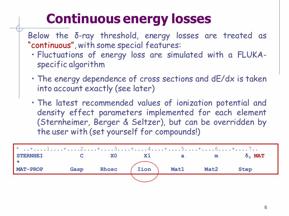
Continuous energy losses Below the δ-ray threshold, energy losses are treated as “continuous”, with some special features: • Fluctuations of energy loss are simulated with a FLUKA-

specific algorithm

• The energy dependence of cross sections and dE/dx is taken into account exactly (see later)

• The latest recommended values of ionization potential and density effect parameters implemented for each element (Sternheimer, Berger & Seltzer), but can be overridden by the user with (set yourself for compounds!)

* ..+....1....+....2....+....3....+....4....+....5....+....6....+....7..

STERNHEI C X0 X1 a m δ0 MAT

*

MAT-PROP Gasp Rhosc Iion Mat1 Mat2 Step

Ionization fluctuations -I

7

The Landau distribution is limited in several respects:

• Maximal energy of δ ray is assumed to be infinite, therefore

cannot be applied for long steps or low velocities;

• Cross section for close collisions is assumed to be equal for all

particles;

• Fluctuations connected with distant collision are neglected,

therefore they cannot be applied for small steps;

• Incompatible with explicit δ ray production.

The Vavilov distribution overcomes some of the landau limitations,

but is difficult to compute if the step length or the energy are not

known a priori.

Ionization fluctuations -II

8

The FLUKA approach:

• Based on general statistical properties of the cumulants of a

distribution (in this case a Poisson distribution convoluted

with dσ/dE);

• Integrals can be calculated analytically and exactly a priori

(min. CPU time);

• Applicable to any kind of charged particle, taking into

account the proper spin dependent cross section for δ ray

production;

• The first 6-moments of the energy loss distribution are

reproduced: n

n xxk

Ionization fluctuations -III

9

Experimental 1 and calculated energy loss distributions for 2 GeV/c positrons (left) and protons (right) traversing 100μm of Si

J.Bak et al. NPB288, 681 (1987)

Nuclear stopping power ( NEW)

Besides Coulomb scattering with atomic electrons, particles undergo Coulomb scattering also with atomic nuclei

The resulting energy losses, called nuclear stopping power, are smaller than the atomic ones, but are important for

Heavy particles (i.e. ions)

Damage to materials (NIEL, DPA )

10

dpa: Displacements Per Atom

11

FLUKA generalized particle name: DPA-SCO

Is a measure of the amount of radiation damage in irradiated materials For example, means each atom in the material has been displaced from its 3 dpa site within the structural lattice of the material an average of 3 times

Displacement damage can be induced by all particles produced in the hadronic cascade, including high energy photons. The latter, however, have to initiate a reaction producing charged particles, neutrons or ions.

The dpa quantity is directly related with the total number of defects (or Frenkel pairs):

atoms/cm3

Ni particles per interaction channel i Nf

i Frenkel pairs per channel

i

i

FiNNρ

=dpa1

Damage to Electronics

12

Category Scales with simulated/measured quantity

Single Event effects

(Random in

time)

Single Event Upset (SEU)

High-energy hadron fluence (>20 MeV)* [cm-2]

Single Event Latchup (SEL)

High-energy hadron fluence (>20 MeV)** [cm-2]

Cumulative effects

(Long term)

Total Ionizing Dose (TID)

Ionizing Dose [GeV/g]

Displacement damage

1 MeV neutron equivalent [cm-2] {NIEL}

* Reality is more complicated (e.g., contribution of thermal neutrons)

** Energy threshold for inducing SEL is often higher than 20 MeV

DOSE

SI1MEVNE

HADGT20M

Generalized particle

Energy dependent quantities I

13

Most charged particle transport programs sample the next collision point by evaluating the cross-section at

the beginning of the step, neglecting its energy dependence and the particle energy loss;

The cross-section for δ ray production at low energies

is roughly inversely proportional to the particle energy;

a typical 20% fractional energy loss per step would correspond to a similar variation in the cross section

Some codes use a rejection technique based on the ration between the cross section values at the two

step endpoints, but this approach is valid only for monotonically decreasing cross sections.

Energy dependent quantities II

14

FLUKA takes in account exactly the continuous energy dependence of:

Discrete event cross section

Stopping power

Biasing the rejection technique on the ratio between the cross section value at the second endpoint ant its

maximum value between the two end point energies.

Ionization fluctuation options

15

Ionization fluctuations are simulated or not depending on the DEFAULTS used. Can be controlled by the IONFLUCT card:

RememberRemember alwaysalways thatthat δδ--rayray productionproduction isis controlledcontrolled independentlyindependently andand cannotcannot bebe switchedswitched offoff forfor ee++/e/e-- (it(it wouldwould bebe physicallyphysically meaningless)meaningless)

* ..+....1....+....2....+....3....+....4....+....5....+....6....+....7..

IONFLUCT FlagH FlagEM Accuracy Mat1 Mat2 STEP

Heavy ions

Ionization energy losses

Up-to-date effective charge parameterizations

Energy loss straggling according to:

“normal” first Born approximation

Charge exchange effects (dominant at low energies, ad-hoc model developed for FLUKA)

Mott cross section

Nuclear form factors (high energies)

Direct e+/e- production

16

Heavy ions dE/dx

17

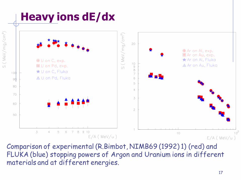
Comparison of experimental (R.Bimbot, NIMB69 (1992) 1) (red) and FLUKA (blue) stopping powers of Argon and Uranium ions in different materials and at different energies.

Bragg peaks vs exp. data: 20Ne @ 670 MeV/n

18

Dose vs depth distribution for 670 MeV/n 20Ne ions on a water phantom. The green line is the FLUKA prediction. The symbols are exp data from LBL and GSI.

Fragmentation products

Exp. Data Jpn.J.Med.Phys. 18, 1,1998

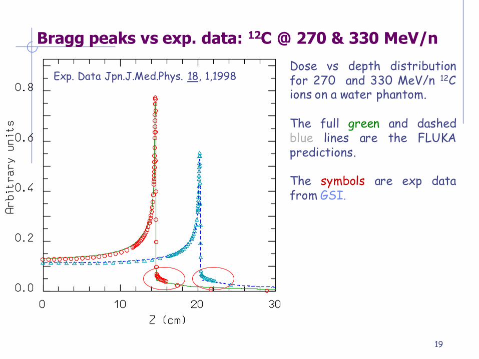
Bragg peaks vs exp. data: 12C @ 270 & 330 MeV/n

19

Dose vs depth distribution for 270 and 330 MeV/n 12C ions on a water phantom. The full green and dashed blue lines are the FLUKA predictions. The symbols are exp data from GSI.

Exp. Data Jpn.J.Med.Phys. 18, 1,1998

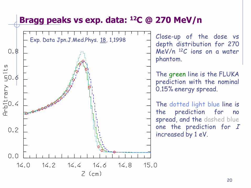
Bragg peaks vs exp. data: 12C @ 270 MeV/n

20

Close-up of the dose vs depth distribution for 270 MeV/n 12C ions on a water phantom. The green line is the FLUKA prediction with the nominal 0.15% energy spread. The dotted light blue line is the prediction for no spread, and the dashed blue one the prediction for I increased by 1 eV.

Exp. Data Jpn.J.Med.Phys. 18, 1,1998

Charged particle transportCharged particle transport

22

Setting particle transport threshold

Hadron and muon transport thresholds are set with this card (see the manual for details);

The neutron threshold has a special meaning (as shown in the low energy neutron lecture), leave at the default value (1 x 10-5 eV);

Warning: the behavior of PART-THR for neutrons has changed with the 2008 release!!

The threshold for nbar’s and neutral kaons should always be zero.

* ..+....1....+....2....+....3....+....4....+....5....+....6....+....7..

PART-THR Thresh Part1 Part2 Step

23

Charged particle transport

Besides energy losses, charged particles undergo scattering by atomic nuclei. The Molière multiple scattering (MCS) theory is commonly used to describe the cumulative effect of all scatterings along a charged particle step. However

Final deflection wrt initial direction

Lateral displacement during the step

Shortening of the straight step with respect to the total trajectory due to “wiggliness” of the path (often referred to as PLC, path length correction)

Truncation of the step on boundaries

Interplay with magnetic field

MUST MUST all be accounted for accurately, to avoid artifacts like unphysical distributions on boundary and step length dependence of the results

24

The FLUKA MCS Accurate PLC (not the average value but sampled from a

distribution), giving a complete independence from step size

Correct lateral displacement even near a boundary

Correlations:

PLC lateral deflection

lateral displacement longitudinal displacement

scattering angle longitudinal displacement

Variation with energy of the Moliere screening correction

Optionally, spin-relativistic corrections (1st or 2nd Born approximation) and effect of nucleus finite size (form factors)

Special geometry tracking near boundaries, with automatic control of the step size

On user request, single scattering automatically replaces multiple scattering for steps close to a boundary or too short to satisfy Moliere theory. A full Single Scattering option is also available.

Moliere theory used strictly within its limits of validity

combined effect of MCS and magnetic fields

The FLUKA MCS - II

As a result, FLUKA can correctly simulate electron backscattering even at very low energies and in most cases without switching off the condensed history transport (a real challenge for an algorithm based on Moliere theory!);

The sophisticated treatment of boundaries allows also to deal successfully with gases, very thin regions and interfaces;

The same algorithm is used for charged hadrons and muons.

Single Scattering

In very thin layers, wires, or gases, Molière theory does not apply.

In FLUKA, it is possible to replace the standard multiple scattering algorithm by single scattering in defined materials (option MULSOPT).

Cross section as given by Molière (for consistency)

Integrated analytically without approximations

Nuclear and spin-relativistic corrections are applied in a straightforward way by a rejection technique

27

Electron Backscattering

Energy

(keV)

Material

Experim.

(Drescher et al 1970)

FLUKA

Single scattering

FLUKA

Multiple scattering

CPU time single/mult ratio

9.3

Be 0.050 0.044 0.40 2.73

Cu 0.313 0.328 0.292 1.12

Au 0.478 0.517 1.00

102.2

Cu 0.291 0.307 0.288 3.00

Au 0.513 0.502 0.469 1.59

Fraction of normally incident electrons backscattered out of a surface. All statistical errors are less than 1%.

28

User control of MCS

Allows to optimize the treatment of multiple Coulomb scattering;

Not needed in shielding problems, but important for backscattering and precision dosimetry;

Can be tuned by material;

Special feature: possibility to suppress multiple scattering (applications: gas Bremsstrahlung, proton beam interactions with residual gas);

Also very important: used to request transport with single scattering (CPU demanding, but affordable and very accurate at low electron energies, can be tuned x material!)

* ..+....1....+....2....+....3....+....4....+....5....+....6....+....7..

MULSOPT Flag1 Flag2 Flag3 Mat1 Mat2 StepSDUM

29

Control of step size

Comparison of calculated and experimental depth-dose profiles, for 0.5 MeV e- on Al, with three different step sizes. (2%, 8%, 20%) Symbols: experimental data. r0 is the csda range

Step size is fixed by the corresponding percentage energy loss of the particle

Thanks to FLUKA mcs and boundary treatment, results are stable vs. (reasonable) step size

30

Control of step size II

Step sizes are optimized by the DEFAULT settings. If the user REALLY needs to change them with: DEstep should always be below 30%

• In most routine problems, a 20% fraction energy loss gives satisfactory results. For dosimetry, 5-10% should be preferred.

WARNING : if a magnetic field is present, it is important to set also a maximum absolute step length and possibly a precision goal for boundary crossing by means of command STEPSIZE (see later)

For EM

For Had/μ

* ..+....1....+....2....+....3....+....4....+....5....+....6....+....7..

EMFFIX Mat1 DEstep1 Mat2 DEstep2 Mat3 DEstep3

* ..+....1....+....2....+....3....+....4....+....5....+....6....+....7..

FLUKAFIX DEstep Mat1 Mat2 Step

31

Magnetic field tracking in FLUKA

FLUKA allows for tracking in arbitrarily complex magnetic fields. Magnetic field tracking is performed by iterations until a given accuracy when crossing a boundary is achieved.

Meaningful user input is required when setting up the parameters Meaningful user input is required when setting up the parameters defining the tracking accuracydefining the tracking accuracy...

Furthermore, when tracking in magnetic fields FLUKA accounts for: The precession of the mcs final direction around the particle direction: this

is critical in order to preserve the various correlations embedded in the FLUKA advanced MCS algorithm

The precession of a (possible) particle polarization around its direction of motion: this matters only when polarization of charged particles is a issue (mostly for muons in Fluka)

The decrease of the particle momentum due to energy losses along a given step and hence the corresponding decrease of its curvature radius. Since FLUKA allows for fairly large (up to 20%) fractional energy losses per step, this correction is important in order to prevent excessive tracking inaccuracies to build up, or force to use very small steps

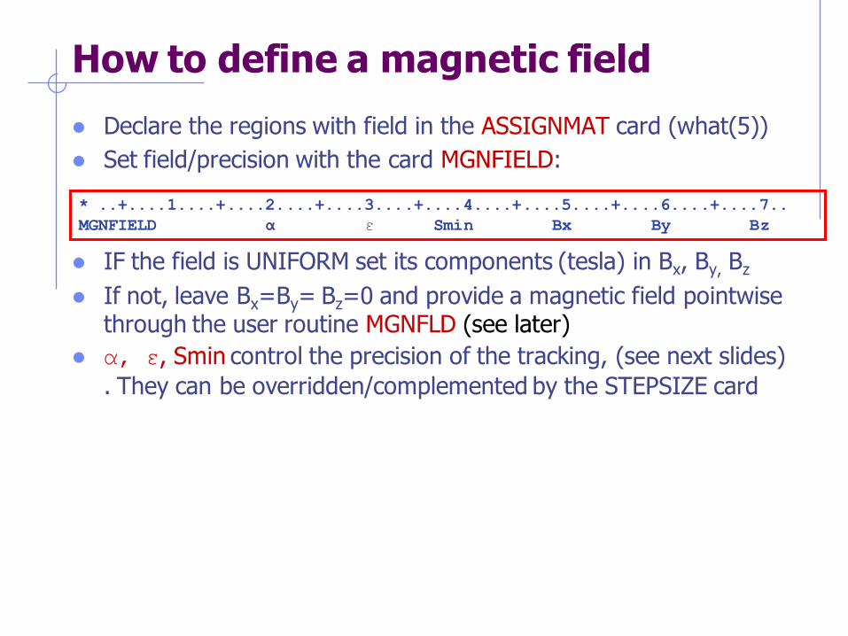
How to define a magnetic field

Declare the regions with field in the ASSIGNMAT card (what(5))

Set field/precision with the card MGNFIELD:

IF the field is UNIFORM set its components (tesla) in Bx, By, Bz

If not, leave Bx=By= Bz=0 and provide a magnetic field pointwise through the user routine MGNFLD (see later)

α, ε, Smin control the precision of the tracking, (see next slides)

. They can be overridden/complemented by the STEPSIZE card

* ..+....1....+....2....+....3....+....4....+....5....+....6....+....7..

MGNFIELD α ε Smin Bx By Bz

33

Magnetic field tracking in FLUKA

The red line is the path actually followed, the magenta segment is the last substep, shortened because of a boundary crossing

= max. tracking angle (MGNFIELD) = max. tracking/missing error (MGNFIELD or STEPSIZE) ‘ = max. bdrx error (MGNFIELD or STEPSIZE)

The true step (black) is approximated by linear sub-steps. Sub-step length and boundary crossing iteration are governed by the required tracking precision

The end point is ALWAYS on the true path, generally NOT exactly on the boundary, but at a distance < ‘ from the true boundary crossing (light blue arc)

34

Setting the tracking precision I

largest angle in degrees that a charged particle is allowed to

travel in a single sub-step. Default = 57.0 (but a maximum of 30.0 is recommended!)

upper limit to error of the boundary iteration in cm ( ’ in fig.). It also sets the tracking error . Default = 0.05 cm

IF and/or are too large, boundaries may be missed ( as in the plot); IF they are too small, CPU time explodes.... Both and conditions are fulfilled during tracking. Set them according to your problem Tune by region with the STEPSIZE card Be careful when very small regions exists in your setting : must be smaller than the region dimensions!

* ..+....1....+....2....+....3....+....4....+....5....+....6....+....7..

MGNFIELD α ε Smin Bx By Bz

35

Setting the tracking precision II

Smin minimum sub-step length. If the radius of curvature is so small that the maximum sub-step compatible with is smaller than Smin, then the condition on is overridden. It avoids

endless tracking of spiraling low energy particles. Default = 0.1 cm

Particle 1: the sub-step corresponding to is > Smin -> accept Particle 2: the sub-step corresponding to is < Smin -> increase Smin can be set by region with the STEPSIZE card

* ..+....1....+....2....+....3....+....4....+....5....+....6....+....7..

MGNFIELD α ε Smin Bx By Bz

36

Setting precision by region

Smin: (if what(1)>0) minimum step size in cm Overrides MGNFIELD if larger than its setting;

(if what(1)<0) : max error on the location of intersection with boundary.;

The possibility to have different “precision” in different regions allows to save CPU time.

Smax: max step size in cm. Default:100000. cm for a region without magnetic field, 10 cm without;

Smax can be useful for instance for large vacuum regions with relatively low magnetic field

It should not be used for general step control, use EMFFIX, FLUKAFIX if needed

* ..+....1....+....2....+....3....+....4....+....5....+....6....+....7..

STEPSIZE Smin/ε Smax Reg1 Reg2 Step

37

The magfld.f user routine

This routine allows to define arbitrarily complex magnetic fields:

SUBROUTINE MAGFLD ( X, Y, Z, BTX, BTY, BTZ, B, NREG, IDISC)

Input variables:

x,y,z = current position

nreg = current region

Output variables:

btx,bty,btz = cosines of the magn. field vector

B = magnetic field intensity (Tesla)

idisc = set to 1 if the particle has to be discarded

All floating point variables are double precision ones!

BTX, BTY, BTZ must be normalized to 1 in double precision

Some warnings about scoring:

Every charged particle step ΔΔxx has its length constrained by:

Maximum fractional energy loss (see FLUKAFIXFLUKAFIX)

Maximum step size for that region (see STEPSIZESTEPSIZE)

MCS (or other) physical constraints

Distance to next interaction (nuclear, δ ray etc)

The averageaverage energy loss is computed as a careful integrationcareful integration over the dE/dx vs energy curve and thenthen it is fluctuated a final ΔΔEE is computed and used for scoring resulting in a scored average effective average effective ΔΔE/E/ΔΔx x uniform along that step

The particle energy used for track-length estimators is the average one along the step (E0-ΔE/2)

38

USRBIN track apportioning scoring

39

The energy deposition will be Δl/Δx ΔE

Δl

Δx, ΔE

USRBIN track apportioning scoring

40

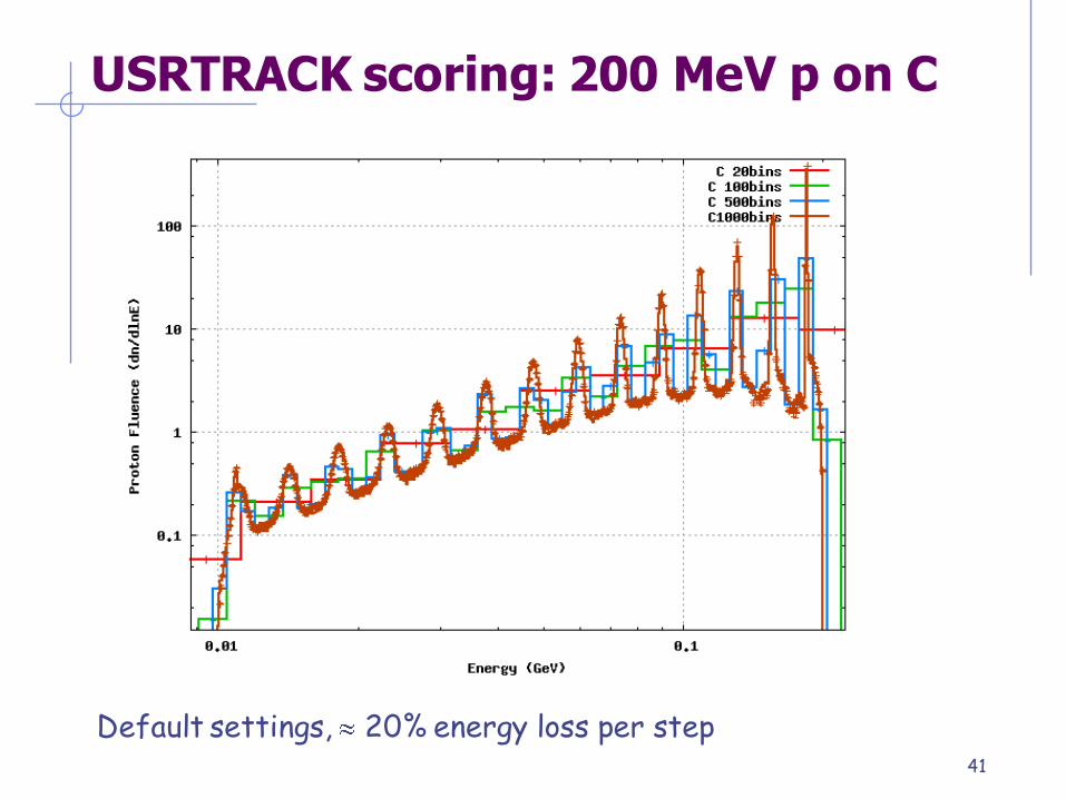
USRTRACK scoring: 200 MeV p on C

41

Default settings, 20% energy loss per step

Ionization Transport Cheat Sheet

42

DELTARAY – Modify Delta-ray effect parameters

STERNHEI - Ionization potential and density effect

MAT-PROP parameters customization

IONFLUCT – Set Ionization fluctuation options

PART-THR - Set particle transport threshold

EMFFIX - Set Step Size control for EM

FLUKAFIX – Set Step Size control for Hadrons/Muons

MGNFIELD - Set magnetic field precision

STEPSIZE - Set stepsize in magnetic field