www.eprg.group.cam.ac.uk

Investment and Efficiency under Incentive

Regulation: The Case of the Norwegian Electricity Distribution Networks

EPRG Working Paper 1306

Cambridge Working Paper in Economics 1310

Rahmatallah Poudineh and Tooraj Jamasb

Abstract

Following the liberalisation of the electricity industry since the early 1990s, many sector regulators have recognised the potential for cost efficiency improvement in the networks through incentive regulation aided by benchmarking and productivity analysis. This approach has often resulted in cost efficiency and quality of service improvement. However, there remains a growing concern as to whether the utilities invest sufficiently and efficiently in maintaining and modernising the networks to ensure long term reliability and also to meet future challenges of the grid. This paper analyses the relationship between investments and cost efficiency in the context of incentive regulation with ex-post regulatory treatment of investments using a panel dataset of 126 Norwegian distribution companies from 2004 to 2010. We introduce the concept of “no impact efficiency” as a revenue-neutral efficiency effect of investment under incentive regulation which makes a firm “investment efficient” in cost benchmarking practice. Also, we estimate the observed efficiency effect of investments in order to compare with no impact efficiency and discuss the implication of cost benchmarking for investment behaviour of network companies.

Keywords Investments, cost efficiency, incentive regulation, distribution

network JEL Classification L43, L51, L94, D21, D23, D24

Contact tooraj.jamasb@durham.ac.ukl Publication April 2013 Financial Support UK ESRC and The Research Council of Norway

(SusGrid - Sustainable Grid Development Project)

Investment and Efficiency under Incentive Regulation:

The Case of the Norwegian Electricity Distribution Networks

Rahmatallah Poudineh

Department of Economics, Heriot-Watt University, UK

Tooraj Jamasb1

Durham University Business School, Durham, UK

April 2013

Abstract

Following the liberalisation of the electricity industry since the early 1990s, many

sector regulators have recognised the potential for cost efficiency improvement in the

networks through incentive regulation aided by benchmarking and productivity

analysis. This approach has often resulted in cost efficiency and quality of service

improvement. However, there remains a growing concern as to whether the utilities

invest sufficiently and efficiently in maintaining and modernising the networks to

ensure long term reliability and also to meet future challenges of the grid. This paper

analyses the relationship between investments and cost efficiency in the context of

incentive regulation with ex-post regulatory treatment of investments using a panel

dataset of 126 Norwegian distribution companies from 2004 to 2010. We introduce

the concept of “no impact efficiency” as a revenue-neutral efficiency effect of

investment under incentive regulation which makes a firm “investment efficient” in

cost benchmarking practice. Also, we estimate the observed efficiency effect of

investments in order to compare with no impact efficiency and discuss the

implication of cost benchmarking for investment behaviour of network companies.

Keywords: Investments, cost efficiency, incentive regulation, distribution network

JEL classification: L43, L51, L94, D21, D23, D24

1 Corresponding author: Durham University Business School, 23/26 Old Elvet, Durham DH1 3HY, United

Kingdom, Phone: +44 (0)191 33 45463, Email: tooraj.jamasb@durham.ac.uk. The authors are grateful to

Luis Orea for very valuable comments on this paper. Financial support from UK ESRC and The Research

Council of Norway (SusGrid - Sustainable Grid Development Project) are gratefully acknowledged.

EPRG 1306

1

1 Introduction

In recent years, achieving a sustainable energy sector, security of supply, and reliability of

service have emerged as overarching energy policy objectives in many countries. A

sustainable energy economy is highly dependent on decarbonising the electricity sector.

Meanwhile, further electrification of the economy is generally regarded as desirable for a

sustainable energy-economy. These goals are pursued through large scale deployment of

renewable energy sources, more efficient use of energy, and active participation of the

demand side.

Achieving the above goals requires a transformation of the electricity networks through

expansion of grids, adoption of new technologies for managing the variability of the supply

side, accommodating an active demand side, and focused research and development. Such

transformation can only be reached through substantial capital investments. Given the

anticipated scale of the required investments in the coming years, ensuring sufficient and

efficient investments in the networks presents itself as a policy and regulatory priority.

Following the liberalisation of the electricity industry since the early 1990s, many sector

regulators have recognised the potential for cost efficiency improvement in the networks

through incentive regulation aided by benchmarking and productivity analysis. Although,

benchmarking has achieved efficiency (mainly in operating costs) new challenges have

emerged as how to address the issue of network investments. The problem is whether a

system of regulation can be designed that provides right incentives for delivery of cost

effective services while ensuring there is no systematic underinvestment or overinvestment.

Hence, regulators need to balance the cost and risk of underinvestment against the cost of

overinvestment in maintaining and modernising the networks. The incentive regulation

accentuates static cost efficiency while investment is a dynamic and long term activity. On

the other hand, benchmarking is a relative concept in the sense that firm’s efficiency depends

not only on its own performance but also on the performance of other companies. The

paradoxical effect of incentive regulation concerning investment and the peculiar

specifications of benchmarking total costs complicate the relationship between investment

and cost efficiency under the incentive regulation with ex-post regulatory treatment of

investment cost.

This paper analyses the relationship between cost efficiency and investments under incentive

regulation with ex-post regulatory treatment of capital expenditure using the case of Norway.

The contribution of this paper is two-folded. Firstly, we introduce the concept of “no impact

efficiency” as a revenue-neutral efficiency effect of investment under incentive regulation

which makes the firm “investment efficient” and immune from cost disallowance in

benchmarking process. Secondly, we estimate the “observed” efficiency effect of investment

in order to compare with no impact efficiency and hence; discuss the implication of cost

benchmarking for the investment behaviour of distribution companies in Norway. Despite the

important role of regulatory treatment of capital expenditure, using benchmarking total costs,

for investments behaviour and efficiency improvement in the networks, the topic has not been

formally studied in the empirical literature.

EPRG 1306

2

The next Section discusses the relationship between network investments and incentive

regulation with reference to the Norwegian regulation regime. Section 3 describes the

methodology used to conceptualise the efficiency implications of investment under incentive

regulation and also presents the stochastic frontier analysis procedure. The empirical results

are presented and discussed in Section 4. Finally, Section 5 is the conclusions.

2 Investment and regulation

Electricity networks are regulated natural monopolies and investments by network companies

are not governed by market mechanisms where decisions are normally based upon expected

higher returns than the incurred cost of capital. In a regulated environment such as the

electricity networks, the investment behaviour of firms is strongly influenced by the

regulatory framework and institutional constraints (Vogelsang, 2002; Crew and Kleindorfer,

1996). The low-powered regulatory regimes such as pure “rate of return regulation” are often

associated with poor incentive for efficiency. Averch-Johnson (1962) showed that regulated

monopolies have an incentive to overinvest when the allowed rate of return is higher than the

cost of capital.

The Incentive-based regimes such as price or revenue caps aim to overcome the efficiency

problem by decoupling prices from utilities’ own costs. However, they give rise to new

challenges regarding the level of investments. The issue of cost efficiency at the expense of

investments or service quality has been discussed in the literature (see e.g., Giannakis et al.,

2005; Rovizzi and Thompson, 1995; Markou and Waddams Price, 1999). Also, when rewards

and penalties are weak or uncertain, the incentive for cost reductions outweighs the

inducement to maintain quality of service and investment. Furthermore, implementing

incentive regulation is complicated and evaluation of the associated efficiency is more

difficult than it is often implied (Joskow, 2008).

The empirical evidence concerning investment behaviour of companies under incentive

regime is not conclusive. While some initially argued that incentive regulation leads to

underinvestment, the later empirical works demonstrated that the outcome of the incentive

regulation concerning the investment behaviour can be in either direction. Waddam Price et

al. (2002), state that a high-powered incentive regulation might lead to overinvestment.

Roques and Savva (2009) argue that a relatively high price cap can encourage investment in

cost reduction as in an unregulated company. Nagel and Rammerstorfer (2008) showed that a

strict incentive regulation regime is more likely to create disincentive for investments.

However, it is generally agreed that in incentive regimes, due to separation of firms’ own cost

from prices, the motivation for cost reducing investment is higher than under the rate of

return regulation (Ai and Sappington, 2002; Greenstein et al., 1995).

Thus, the main challenge of the regulator is to choose the right incentives in order to prevent

any systematic overcapitalisation or underinvestment. The ability to disallow excessive costs

can help regulators achieve more efficient levels of investment which otherwise firms would

EPRG 1306

3

tend to overinvest in risky projects (Lyon and Mayo, 2005). However, following periods of

cost disallowances there is a greater possibility of disincentive for investments.

The regulatory opportunistic behaviour is also a concern for the regulated firm as it

introduces uncertainty into the regulatory contract. Gal-Or and Spiro (1992), for example,

argue that a sudden shift in regulatory regime which allows for the use of cost disallowance

instruments will decrease the propensity to invest. Regulatory uncertainty is an important

issue in network industries such as electricity networks and can have serious implications for

investments. This is because under uncertainty, delaying investments may be beneficial even

though a project may indeed recover its capital costs (Dixit and Pindyck, 1994). There is also

non-regulatory uncertainty, such as future demand, that the regulated company needs to take

into consideration when deciding to invest.

From the regulatory viewpoint, it is important that decisions influencing the investments of

the firms are based upon economic efficiency. For example, the cost of reducing service

interruptions through investments should be lower than the socio-economic costs of service

interruption. In effect, the regulator seeks an efficient level of investment in the grid although

realising this goal through regulation is a challenging task. This is because theory does not

provide clear indications of the conditions under which “efficient” levels of investment are

achieved and what factors lead to over and underinvestment (von Hirschhausen, 2008).

Moreover, the empirical evidence from cases of overinvestment or underinvestment is rare.

Therefore, the outcome of incentive regulation regarding investments is ambiguous, and that

regulators in practice tend to adopt a combination of different regulatory incentive

mechanisms in order to achieve their objectives.

2.1 Power sector reform and network regulation in Norway

Norway was among the first countries, after Chile and the UK, to embark on power sector

reform by unbundling the different elements of electricity industry across the value chain.

This means generation and retail supply which are potentially competitive were separated

from the transmission and distribution that are natural monopolies. Hence; the distribution

and transmission networks are subject to regulation. The Norwegian Water Resource and

Energy Directorate (NVE) were appointed as the sector regulator since Norwegian Energy

Act came into effect in 1991. Unlike the other countries where regulatory reform was often

accompanied by transfer of ownership, the Norwegian power industry mainly remained under

the state or local municipalities’ control after reform. Also, companies that involve in both

monopolistic (distribution or regional transmission) and competitive business (generation or

retail supply) are required to keep them separated either legally and/or financially2.

2 In 2010, about 67 companies were involved in generation, grid operation, and supply to end users. Vertically

integrated companies with more than 100,000 customers are obliged to separate their monopolistic operation

from competitive activities (legal unbundling). The Energy Act requires the integrated companies to keep

separate accounts for their monopolistic and competitive businesses (NVE, 2010).

EPRG 1306

4

At the early years of the reform, there were approximately 230 distribution networks and 70

generation units in Norway. The high number of utilities reflects the dispersed nature of

hydroelectric resources as the main source of power generation as well as the historical

development of the sector in the country. In December 2010, around 167 companies were

engaged in gird operation (NVE, 2010). The marked reduction in the number of distribution

companies is the result of mergers and acquisitions among network companies in pursuit of

scale efficiency gains.

After the reform, initially the distribution companies were operating under the rate of return

regulation. However, due to lack of incentives for cost efficiency, since 1997, the regulatory

regime was changed to incentive regulation. From 2007, NVE implemented a new regulatory

model which also uses Data Envelopment Analysis (DEA) as an efficiency benchmarking

method. The companies are regulated with a revenue cap regime that covers their costs

annually based on their distance from the efficient frontier (best practice) in the sector.

2.2 Investments under Norwegian regulatory regime

A feature of the Norwegian incentive regulation is to prevent systematic overinvestment or

underinvestment in the networks. The incentives are provided through a combination of

economic and direct regulation (NordREG, 2011). Along with the profit motivation, the

network companies need to undertake substantial investments in order to meet their

obligations as stated in the Energy Act. For example, Section 3-4 of amended Energy Act

states that distribution companies are obliged to connect new generation sources and

consumers that are not covered by the supply requirement.

Moreover, distribution companies are incentivised to maintain a high level of quality of

service. The cost of network energy losses and cost of energy not supplied (CENS) due to

interruptions or capacity constraints in the grid are incorporated in the regulatory model so

that the firms take them into account. Therefore, firms normally should not have an incentive

to tune out their reinvestments as this would increases their total costs due to deterioration of

their quality of service over time. In addition, a profit incentive is provided through a

minimum guaranteed return on capital. The regulation states that all companies should

achieve a reasonable (minimum 2%) return on capital, given effective management,

utilization, and development of the networks3. Similarly, overinvestment will increase the

total costs and will negatively affect their relative efficiency in the cost benchmarking

exercise which will impact their revenue adversely.

Figure 1 shows total investments, new investments, and reinvestments by the distribution

companies between 2004 and 2010. As shown, total investments are strictly increasing since

2006. The investment data indicates that the source of investment increase is reinvestment

and not the new investments. Although new investments remained almost constant, they have

3 Any network company that falls below this minimum level will receive a correction in its revenue so that they

achieve a minimum 2% return on capital. The normal return for Norwegian distribution companies is currently

5.62%.

EPRG 1306

5

had a higher share in total investments than reinvestments. For instance, 68% of the

investments observations during the period of study have a share of new investments to total

investments that is higher than 50%. This can be an indication of strong investment

incentives which have motivated the networks to undertake new investments, possibly

beyond their minimum reinvestment needs. Such a change can be attributed to the regulator’s

view in recent years that social costs of underinvestment are higher than social benefits of

overinvestment (Helm and Thompson, 1991).

Figure 1: Investments in Norwegian distribution companies

3 Methodology

In this Section, we first present a model of the incentive regulation of electricity distribution

networks in Norway and then analyse the relationship between investments by the utilities

and change in their relative efficiency under incentive scheme. We then describe the

econometric approach and the models estimated in order to explore the efficiency effects of

investments.

3.1 Modelling Incentive Regulation

The allowed revenues of regulated networks are determined by incentive regulation and cost

efficiency benchmarking. Within this framework, investments are encumbered indirectly

such that overinvestment can result in partial disallowance of investment costs. The

Norwegian regulator computes the allowed revenue ( ) of the firms using Equation (1),

which, in essence, is the generic incentive regulation formula representing the trade-off

between cost reduction incentive and rent transfer to the consumer, given the presence of

asymmetric information between the firm and the regulator (Newbery, 2002; Joskow, 2005).

EPRG 1306

6

(1)

Where is the actual (own) costs of a network company, is the norm cost obtained by

using the frontier-based benchmarking method Data Envelopment Analysis (DEA), and is

the power of incentive in terms of the weight given to benchmarked costs vs. actual costs in

setting the allowed revenue. The power of incentive is important for motivating the firms to

move as close as possible to their norm (benchmarked) cost as they lose revenue when

deviating from the efficient frontier. The share of actual costs and norm costs in determining

the revenue caps is currently 40 and 60% respectively (i.e. ). Placing more weight on

norm costs increases the incentive power of regulation and promotes indirect competition

among the utilities to improve their cost efficiency relative to best practice.

Actual costs include operating and maintenance costs, capital costs, and depreciation costs. In

addition, the regulator deducts the cost of energy not supplied (CENS) from the firms’

revenue cap4 and adjusts the allowed revenue for tax and other non-controllable expenses.

The regulator uses data with a two year lag which is updated with an inflation index. The

allowed revenue is then corrected at the end of the year when final actual data becomes

available5.

We divide both sides of (1) with and rearrange such that it yields:

(2)

where

is the firms’ efficiency in period . When a firm invests the amount , this

will impact its revenue by changing its relative efficiency in cost benchmarking. The

variables for before and after undertaking investments are denoted by subscripts 1 and 2

respectively. The change in a firm’s revenue due to an investment can be computed from

equation (3).

(3)

The change in actual cost of the firms after undertaking investments is equal to the amount of

investments ( ). We substitute for in the bracket and rearrange (3) as

presented in (4) to show the change in revenue as a result of investments.

(4)

Revenue effect of investments due to benchmarking

4 In order to incentivise network companies to improve service quality.

5 While the current and previous year investments (years t and t-1) are not included in the regulatory asset base

(RAB) due to a time-lag, the companies can start to calculate a return on investment into their allowed revenue

(i.e. tariff base) from the commissioning year.

EPRG 1306

7

Equation (4) presents the main framework for the network companies’ incentive to undertake

investments. In the absence of cost benchmarking (i.e. when ) the firm would

automatically earn a return on its investments because the change in the firm’s revenue is the

same as the change in its cost ( ), and the company can pass all its investment costs

to its customers. However, as investments are included in cost benchmarking, the firms’

revenue also depends on their relative cost efficiency before investments ( ) and after

investments ( ). This is reflected in the second component of (4), to which we refer as in

(5), and shows the (gross) revenue effect of investments due to benchmarking.

(5)

As seen from (5), the revenue effect of investments consists of two parts. Clearly, we always

have . However, the outcome of the component of (5) is not certain as

it is not clear whether, following an investment, the cost efficiency increases, decreases, or

remains constant6.

Depending on the initial and after investment measured cost efficiency, can take different

values. If , the firm gains less from investing compared to the case of no cost

benchmarking (ceteris paribus). However, when , investment costs are fully recovered

as there is no benchmarking. If , investment creates synergy by excessive increase in

efficiency although this may not happen under normal condition7 so in most situations one

expects .

(6)

Thus, as shown in (6), the change in revenue after investments is not necessarily equal to the

change in cost and it crucially depends on the value that takes. Although the revenue also

depends on the power of incentive ( ), it is a predetermined parameter which is beyond the

control of the firm. Thus, the feasible outcome can only be achieved when and

benchmarking has no adverse impact on the firms’ revenue. - i.e. when the efficiency after

investments increases (due to productivity of capital) to an amount that results in (note

that also when the firm is on the efficient frontier and remains there after investments we

have and consequently becomes zero). This efficiency can be obtained by

solving (5) with respect to as in (7).

(7)

Equation (7) shows how the Norwegian incentive regulation links investments to efficiency

improvement. In order for a firm to earn a profit on its investments as if there was no cost

benchmarking (ceteris paribus), its efficiency should be, at least,

after the investment.

6 .

7 The reason is that if the share of investments to other costs (before investments) increases, the efficiency

required to satisfy the inequality rises considerably. However, under certain circumstance we can have

which we refer to it in Section 4.

EPRG 1306

8

An efficiency level below this will result in lower revenue relative to the no benchmarking

case. We use the term ‘no impact efficiency’ to refer to the ‘revenue-neutral efficiency effect

of investment under cost benchmarking as presented in (7). In other words, a firm is

considered ‘investment efficient’ when it meets the ‘no impact efficiency’ criteria under

regulation8.

The Norwegian incentive regulation links investment and efficiency to ensure that firms do

not undertake undue investments. This means that the regulator does not need to interfere in

the firms’ investment decisions, but indirectly incentivises them to be investment efficient. A

limit analysis of (7) shows that as increases, the efficiency will approach . The

opposite of this implies that when the ratio of investment to other cost9 increases, the firm

needs to achieve a higher efficiency level (which in limits is equal to unity) in order to avoid

revenue loss. This means that the expected interval of the no impact efficiency change is

, which depending upon the investment to cost ratio would be closer to

lower or upper boundary.

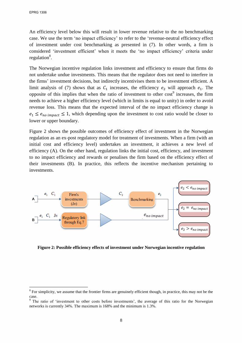
Figure 2 shows the possible outcomes of efficiency effect of investment in the Norwegian

regulation as an ex-post regulatory model for treatment of investments. When a firm (with an

initial cost and efficiency level) undertakes an investment, it achieves a new level of

efficiency (A). On the other hand, regulation links the initial cost, efficiency, and investment

to no impact efficiency and rewards or penalises the firm based on the efficiency effect of

their investments (B). In practice, this reflects the incentive mechanism pertaining to

investments.

Figure 2: Possible efficiency effects of investment under Norwegian incentive regulation

8 For simplicity, we assume that the frontier firms are genuinely efficient though, in practice, this may not be the

case. 9 The ratio of ‘investment to other costs before investments’, the average of this ratio for the Norwegian

networks is currently 34%. The maximum is 168% and the minimum is 1.3%.

EPRG 1306

9

3.2 Modelling a Stochastic Efficient Frontier

This section presents the efficiency measurement techniques and empirical model estimated

in this study. We estimate the efficiency of firms before and after investments and use the

efficiencies to calculate the ‘no impact efficiency’ for current investment levels of the

networks. We use an input distance function which allows us to estimate the efficiency of the

firms when input price data is not available (Färe and Lovell, 1978; Coelli, 1995). Other

advantages of distance functions are that they do not depend on explicit behavioural

assumptions such as cost minimization or profit maximization and they can accommodate

multiple inputs and outputs (Kumbhakar and Lovell 2000; Coelli et al., 2005).

Input distance functions have been used in empirical studies for efficiency and productivity

analysis of industrial units as in Abrate and Erbetta (2010) and Das and Kumbhakar (2012) as

well as those of electricity networks such as Tovar et al. (2011), Hess and Cullmann (2007),

and Growitsch et al. (2012). The output of electricity networks is determined exogenously by

demand for energy and connection thus companies can only adjust inputs (i.e. costs) to

deliver a given service efficiently.

An input distance function can be defined as in (8):

{ (

) } (8)

where represents the input vectors that produce the output vector , and indicates a

proportional reduction in input vector. The function has the following characteristics: (i) it is

linearly homogenous in , (ii) it is non-decreasing in and non-increasing in , (iii) it is

concave in and quasi-concave in , and (iv) if then and if is on

the frontier of input set.

Input-oriented technical efficiency can be obtained from (9):

, (9)

This means that technical efficiency is defined as the inverse of the distance function. When a

firm is operating on the frontier it shows a distance function value equal to unity and

consequently has a technical efficiency score of 1. The general form of an input distance

function is as in (10):

∑

∑ ∑

∑

∑ ∑

∑ ∑

EPRG 1306

10

where represents the distance function, is output, is input, represents time

trend, subscript i=1…N denotes the number of the firms, and t=1…T indicates number of

years. Also, and show the number of outputs and inputs respectively.

Parameters , , and are to be estimated.

Condition of homogeneity of degree one in input is imposed by the following constraints:

∑

∑

and

∑

Symmetry condition is met if:

(11)

We transform the input distance function into econometric models to be estimated by the

stochastic frontier analysis (SFA) method and to obtain technical efficiency of the firms.

Imposing the homogeneity of degree one by deflating inputs by th input (we use

other cost ( ) to deflate) will lead to (12):

(12)

where is the translog functional form. For the purpose of estimation we rearrange the

above equation as:

(13)

where represents the non-negative technical inefficiency. The error components

have the following distributions.

and

(14)

is a normally distributed random error term and is a half-normal heteroscedastic

random error term that capture inefficiency. As the efficiency is affected by the investments

we model the heteroscedastic inefficiency variance ( as in (15).

(15)

where and are parameters that needs to be estimated and is normalised investment

level with respect to sample median. As shown in (16) we can separate the heteroscedastic

variance into its homoscedastic component ( ) and the element related to investments.

EPRG 1306

11

( )

(16)

This allows us to purge the effect of investments on inefficiency as seen from (17). In terms

of estimation, equations (13) and (15) are estimated simultaneously based on the only

observed data in (13). Having estimated them, homoscedastic inefficiency can be easily

obtained as follows:

(17)

It is clear that | where , On the other hand, thus

we can write:

(18)

where, is before-investment inefficiency and is after-investment inefficiency

( ). The firm specific technical efficiency is then computed by and

. The “no impact efficiency” is calculated using Equation (7).

3.3 Data

We use a dataset comprising a weakly balanced panel of 126 distribution companies from

2004 to 2010. All the monetary data are in real terms adjusted to 2010 price level. Our

distance function model consists of two inputs and two outputs. The inputs are capital

expenditure ( ) and other costs ( ). Following the Norwegian regulatory approach, we

incorporate quality of service into our benchmarking model by adding the cost of negative

externalities (network energy losses and service interruptions) to the directly incurred

elements of operating cost as presented in (19).

(19)

The cost of energy not supplied is calculated from the number minutes of interruptions times

consumer willingness-to-pay for more reliable service.10

The cost of network energy losses is

computed by multiplying the physical losses with average annual system price of electricity

as used by the regulator.

10

Consumer willingness to pay for quality of service is derived from consumer surveys and technical analysis.

EPRG 1306

12

We use “total number of customers” (residential plus recreational homes) and “energy

density” (energy distributed per Km length of network) as outputs. Numbers of customers are

commonly used in efficiency analysis of electricity networks (e.g. Growitsch et al., 2012;

Miguéis et al., 2011). Energy density captures the effect of asset utilisation and network

congestion as cost drivers. Moreover, network reliability and consequently quality of supply

is directly affected by the length of network (Coelli et al., 2010). In addition to the input and

output variables we use three weather and geographical variables to capture the heterogeneity

among the firms11

. These factors can impact cost efficiency of the networks and controlling

for their effects can help to account for unobserved heterogeneity among network utilities

(Growitsch et al., 2011; Jamasb et al., 2012)12

. Table 1 summarises the descriptive statistics

of the data used.

As we use ‘other costs’ ( ) to impose homogeneity of degree one, the dependent variable of

model is . The parameters used in the model are obtained by maximum likelihood

estimation procedure. The optimisation technique used is Berndt-Hall-Hall-Hausman (bhhh)

algorithm. Furthermore, in order to facilitate the interpretation of the first order terms, all

variables are divided by their sample median prior to estimation.

Table 1: Descriptive statistics

Variable Description Variable Name Min. Max. Mean Std. Dev.

Inputs

Other costs* 1205.25 1178987 40075.5 63466.03

Capital expenditures* In 167.11 92899.7 12730.71 16024.87

Outputs

Energy density (MWh/Km) 137.12 6485.25 554.64 515.670

Number of customers (#) 18 515152 12575 25430.4

Geographical variables

Snow condition (millimetres) 53 1193.61 373.99 196.18

Wind / distance to cost (ratio) 0 0.1610 0.0162 0.0288

Forrest productivity (fraction) 0 0.5489 0.1566 0.1199

*Monetary variables are in ‘000 NOK.

11

The three variables are: (1) snow conditions, in millimeters of snow per year at a given temperature (around 0

degrees C), (2) Wind and distance to coast, as a ratio (average extreme wind/distance to coast), and (3) forest

productivity, a number between 0 and 1 showing the share of forest with this growth rate along the power lines. 12

We examined the influence of asset age (ratio of depreciation to book value) as control variable. However, the

variable showed inconsistencies in the sign of the age variable itself as well as for first order terms of other

variables. Other measures of age may produce different results but these were not available. At the same time,

the results indicated that inclusion of age does not change the efficiency scores significantly.

EPRG 1306

13

4 Results and Discussion

The profit motive implies that incentive regulated firms evaluate the cost and benefit of

undertaking investments by comparing a possible reduction and increase in allowed revenue

as a result of efficiency effect of the investments in cost benchmarking. However, the

outcome depends on the net efficiency effect achieved by the investments.

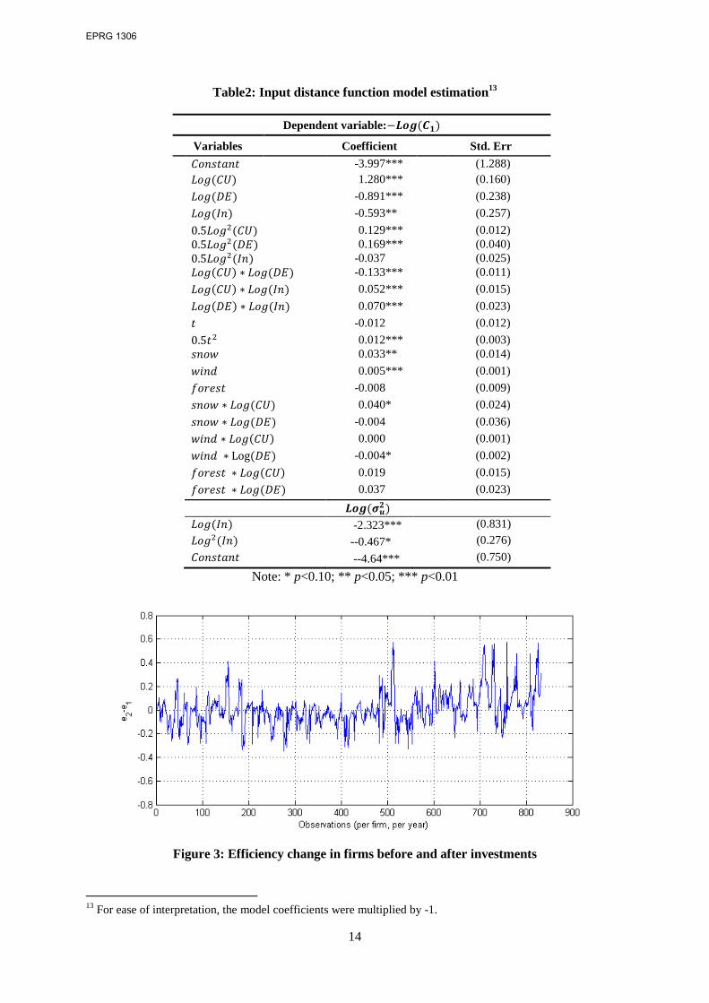
Table 2 presents the results of the input distance function and heteroscedastic variance model

estimations. As shown, the coefficients of first order terms for the number of customers,

energy density and investments are statistically significant and have the expected signs.

These coefficients can be interpreted as distance function elasticity with respect to outputs

and inputs at sample median. The first order coefficients for snow and wind are significant

and consistent in terms of sign which indicate that these geographic variables are cost drivers

as well. However, only one interaction term of wind and snow variables with the outputs is

statistically significant. The heteroscedastic inefficiency variance model shows significant

coefficients both for first order and quadratic terms.

Figure 3 illustrates the changes in the efficiencies before and after investments. As shown,

investments have impacted efficiency of the firms and within a relatively wide range. It is

evident that the impact of investments on the efficiency variation among the firms is not

uniform, in the sense that some of the firms gained while some others lost efficiency. This

complies with the basic notion of ex-post regulatory treatment of investment based on

benchmarking that efficiency effects influence investment behaviour of firms as high

investments involve a risk of efficiency loss.

Figure 4 shows the distribution of efficiency variation following investments. The descriptive

statistics of graph data is presented in Table 3. As seen from the graph and the table, the

change in efficiency tends towards an asymmetrical distribution. The mean of efficiency

variation presented in Table 3 implies that, on average, investment contributed to about 0.8%

efficiency gain. However, the average might not be a very reliable measure for the

performance of the whole sector, as it will be influenced by the outliers. Moreover, as shown

in Table 3, the Jarque-Bera test of normality is rejected and distribution is right skewed. The

maximum positive variation is 0.56 whereas on the negative side it is -0.34. In addition to

implying that an increase in investments is associated with higher efficiency than with

inefficiency, this can also be related to the notion that the fidelity of the estimations decrease

as we begin to move away from the mean. The majority of the observations lie between -15%

to 15% (one standard deviation) efficiency variations following investments.

EPRG 1306

14

Table2: Input distance function model estimation13

Dependent variable:

Variables Coefficient Std. Err

-3.997*** (1.288) 1.280*** (0.160)

-0.891*** (0.238)

-0.593** (0.257)

0.129*** (0.012) 0.169*** (0.040) -0.037 (0.025)

-0.133*** (0.011)

0.052*** (0.015)

0.070*** (0.023)

-0.012 (0.012)

0.012*** (0.003)

0.033** (0.014)

0.005*** (0.001)

-0.008 (0.009)

0.040* (0.024)

-0.004 (0.036)

0.000 (0.001)

-0.004* (0.002)

0.019 (0.015)

0.037 (0.023)

-2.323*** (0.831)

--0.467* (0.276)

--4.64*** (0.750)

Note: * p<0.10; ** p<0.05; *** p<0.01

Figure 3: Efficiency change in firms before and after investments

13

For ease of interpretation, the model coefficients were multiplied by -1.

EPRG 1306

15

Figure 4: The distribution of efficiency change following investments

Table 3: Descriptive statistics of

Mean 0.007968

Median 0.001406

Maximum 0.571541

Minimum -0.348183

Std. Dev. 0.145273

Skewness 0.875255

Kurtosis 5.195926

Jarque-Bera 273.7230

Probability 0.000000

Furthermore, as illustrated by the scatter plot in Figure 5, efficiency loss after investments is

more prevalent among the companies with lower investment to total cost ratios. On the other

hand, those companies with average investment levels show more efficiency gain following

investments compared with companies with very high share of investment in total cost. This

suggests that middle scale investments, typically, have been more productive than the larger

and especially than the small ones. This can be an indication of complexity of investment and

efficiency relation under benchmarking as lower capital expenditure might lead to an increase

of other costs and hence; may not help with efficiency improvement. It also implies that small

scale investments should be better scrutinized before implementation to avoid lower allowed

revenue as a result of cost benchmarking.

EPRG 1306

16

Figure 5: Efficiency change versus investments to cost ratio

Figure 6 summarises the distribution of before investment, after investment and no impact

efficiency estimated in different years. As seen from the figure, in all cases the distributions

do not show zero skewness rather the mass of distribution is concentrated around more

efficient region without a noticeable change over different years. Additionally, the lower

quartile is higher for the case of no impact efficiency compared with before investments and

after investments efficiency, reflecting the fact that given the current level of investment

efficiency improvement is required for many firms.

Table 3 compares the average of the same efficiencies in each year for all companies. As the

table shows, apart from 2006, on average, investment made positive contribution to

efficiency of the sector. However, the average efficiency gained after investment fall behind

no impact efficiency by 1% in 2010 to 4.3% in 2006. The average usually becomes affected

by outliers hence; in order to make a more reliable inference on the performance of sector we

have weighted efficiencies by the share of their corresponding investment in the total

investment of the sector. This is to ensure that the weight effect of firms on the total

investment behaviour of sector is taken into account when looking at the sector level. As it is

shown in Table 3, the difference between before and after investment efficiencies raised to

17%. At the same time, no impact efficiency reduced to reflect the fact that the sector still can

increase the level of investment through new reallocations of investments and without

lowering average efficiency gain of the sector.

EPRG 1306

17

Figure 6: Distribution of efficiencies estimated

EPRG 1306

18

Table 3: Average ‘before investment’, ‘after investment’, and ‘no impact’ efficiency

Efficiency measured 2004 2005 2006 2007 2008 2009 2010

Average of 0.896 0.897 0.902 0.892 0.894 0.892 0.883

Average of 0.905 0.902 0.881 0.902 0.911 0.905 0.905

Average of 0.921 0.923 0.924 0.918 0.923 0.921 0.915

Weighted average

The reallocation of investments can increase total investments in the sector because there are

significant performance discrepancies among the companies as depicted in Figures 3 and 4.

The very efficient firms that surpassed no impact efficiency may wish to increase their

investment levels in order to gain from their efficiency level. The investment increase can be

continued until efficiency after investment reduces to no impact efficiency, in which state,

some form of optimality will be achieved. On the other hand, those firms that their efficiency

after investment falls short of no impact efficiency needs to reduce their investment level in

order to avoid inefficiency associated loss14

. The net effect of new reallocation is an increase

in total investments without reducing the average efficiency of the sector.

As discussed above, the outcome of ex-post regulatory treatment of investments through total

cost benchmarking is that some firms will lose part of their capital cost while some other

recover all their investment and some make above normal profit. For example, the few firms

that appear to have outperformed the investment efficiency requirement – i.e. their efficiency

after investments exceeded the no impact efficiency considerably (the instance of

discussed in Section 3.1) can earn more compared to the no benchmarking case. Under the

circumstance that an “investment efficient frim” gains and an “investment inefficient” loses;

the ex-post regulatory treatment of investment is effective in rewarding efficient and

penalising inefficient firms.

However, this might not always be the case as the condition under which benchmarking

produce reliable results does not always hold. This is because efficiency, in benchmarking

terms, is a relative concept and only reveals information about firm performance in relation to

other firms. Thus, the relative efficiency of a firm can also improve when the peer companies

are not performing well. For instance, when companies are capital productive and their

investments are proportional to their capital productivity, they might move to a higher level

of relative efficiency after investments. However, the same can happen when they

underinvest, something which gives them the appearance of cost efficiency. Therefore, unless

14

In this analysis we ignore the concept of dynamic efficiency hence; we do not take into account cost effect of

investments that takes more than one regulatory period to become realised. This is because our positive analysis

is based on the current form of incentive regulation with ex-post regulatory treatment of investment practiced in

Norway and many other countries.

EPRG 1306

19

the frontier firms genuinely represent the best practice, the results of benchmarking can be

misleading.

The benchmarking limitation regarding investment embraces other cases such as when the

firms’ investments behaviour is harmonised in the sense that they are in the same phases of

their investment cycles. This refers to the case that firms invest in the similar periods and in

proportion to their total cost levels but beyond their capital productivity. As the measure of

efficiency is relative the firms tend to remain in a relatively similar efficiency position before

and after investment. Under this condition, benchmarking fails to identify the incidence of

overinvestment.

The regulator expects that the threat of partial disallowance of capital expenditures built into

the regulatory formula leads the firms towards efficient investments. However; the power of

the model to detect overinvestments is limited to the case of ‘out of phase’ investments (i.e.

when firms are not in the same investment cycle). Thus, sector-wide ‘in phase’ or cyclically

harmonised overinvestments by the firms are not revealed in the process of benchmarking

because the approach is based on between-firms comparisons. This will, in turn, limit the

ability of the regulator to effectively address the issue of overinvestment. Harmonised

investment behaviour can happen when many firms follow a similar investment policy. For

instance, when a regulator guides the investment into a desired direction by, for example,

offering a higher return for investments in innovation and particular types of technologies and

activities (e.g. Smart Grids).

A parallel argument also holds in the case of harmonised underinvestment. This problem

arises when the incentives to invest are not strong enough or the regulation is restrictive

which causes firms to reduce their investments, something which in the short run can give the

appearance of cost efficiency while, overtime, leading to gradual degradation of the networks

and their reliability.

There are some possible remedies to address the cases of harmonised underinvestment or

overinvestment. For instance, the regulator can use the power of incentive ( ) in order to

influence the investment inefficient firms when there is evidence of overcapitalisation. The

higher power of incentive is the greater possibility of financial loss as a result of investment

inefficiency. Thus, a high causes investment inefficient firms to reduce their investments

and consequently improve their efficiency. Also, frontier firms need to follow the same path

to maintain their position on the frontier. At present, is 60% for Norwegian distribution

companies. A small increase in can reduce the net efficiency gains by the firms and create

disincentive for investments. On the contrary, reduction of the power of incentive aligns the

revenue of the firm more with its actual cost and increases propensity to investment.

However, the power of incentive is usually set for a long period of time in order to make the

investment behaviour of firms predictable and provide a stable regulatory environment.

Therefore, the regulator’s ability to modify the power of incentive is limited15

.

15

This strategy can have significant side effects such as inducing uncertainty in regulation. Therefore, it needs

to be used with strong evidence of persistent or systematic over or underinvestment in the sector.

EPRG 1306

20

In order to avoid underinvestment and quality of supply deterioration induced by cost

reduction incentives incorporated in incentive regulation, regulators adopt either quality

performance targets or include the cost of network energy losses and cost of energy not

supplied in benchmarking model as in the case of Norway. This is to ensure that no

systematic underinvestment happens which endangers network reliability over time.

However, the issue is that underinvestment can have an immediate effect on efficiency

improvement whereas its impact on network reliability is lengthy.

Another possible problem of ex-post regulatory treatment of investment using benchmarking

is that it can ease the strategic behaviour for trade-off between Capex and Opex16

in order to

avoid revenue loss from investment inefficiency when firms invest beyond their productive

capacity. For instance, as shown in Table 2, investments and other costs are negatively

correlated in a such way that a 1% increase in investment with respect to median of the sector

can result in 0.59% reduction of other costs. This in turn raises the regulatory issue of

substitution of capital for labour introduced by Averch-Johnson (1962).

To sum up, the relationship between investment and efficiency under incentive regulation

with ex-post regulatory treatment of investment is not straightforward. As efficiency is a

relative concept in economics, performance of a firm is not only related to its own behaviour

but also to that of other firms. The conditions under which overinvestment can reduce cost

efficiency of the firm might not always hold. Moreover, it takes time for underinvestment to

appear as cost in the form of quality of supply deterioration. The Norwegian regulator

attempts to incentivise the companies to operate and maintain their networks in an efficient

manner and provide a high level of reliability. However, the use of cost benchmarking in

order to ensure effective capital expenditures does not necessarily lead to the socio-economic

efficient level of investments.

5 Conclusions

Contrary to the early years of electricity sector reforms when regulators were mainly

concerned with cost efficiency, an emerging and pressing issue is how to ensure sufficient

and efficient level of investments in the regulated networks. Over the years, efficiency of the

natural monopoly power networks has been improving as a result of incentive regulation.

However, the need for significant investments in the future combined with the incentives to

reduce costs gives rise to new challenges regarding the efficiency and sufficiency of

investments in the networks. In this study we analysed the relation between cost efficiency

and investment behaviour of electricity distribution networks under ex-post regulatory

treatment of investments using the case of Norway.

16

Capital expenditures and operational expenditures.

EPRG 1306

21

We introduced the concept of “no impact efficiency” as the revenue-neutral efficiency effect

of investment under cost benchmarking which, if achieved, makes the firm “investment

efficient” and immune from cost disallowance in benchmarking process. Also, we estimated

the observed efficiency effect of investment in order to compare this with no impact

efficiency and discussed the implication of cost benchmarking for the investment behaviour

of distribution companies in Norway.

The results show that the un-weighted average efficiency gain of the sector as a result of

investments is 0.8%. However, when the efficiency variations following investment are

weighted by their share of total investment in the sector; the effect increases to 17%

reflecting the fact that more investment often resulted in higher efficiency. At the same time,

there are significant variations in efficiency gain following investments at the level of

individual companies. The results suggest those firms that fall short of no impact efficiency

need to reduce their capital expenditure in order to improve their efficiency following

investment. On the other hand, the firms that outperformed no impact efficiency may wish to

increase their investment levels in order to gain from the efficiency they achieved. Overall,

the new reallocation of investments increases the total investment of the sector without

lowering the average efficiency gain of the sector.

Efficiency is a relative concept in productivity analysis. Hence, using benchmarking tools to

promote cost efficiency and at the same time to ensure efficient levels of investment can

result in unintended outcomes. The Norwegian incentive regulation scheme is designed to

discourage overinvestment through partial disallowance of capital expenditures built into the

regulatory formula and benchmarking practice. However, the power of the model to detect

overinvestments is limited to the case of ‘out of phase’ investments or non-harmonised

investment behaviour.

Moreover, benchmarking capital expenditures along with the other costs facilitates strategic

behaviour by the firms in the form of trading-off between Capex and Opex in order to avoid

financial loss in the process of revenue setting. Furthermore, systematic underinvestment can

give the appearance of cost efficiency while it can have a negative effect on quality of service

over time. Although underinvestment will eventually be reflected in the companies’ cost of

energy not supplied and cost of network energy losses, it can take some time for this effect to

become apparent while the cost and efficiency improvement effect of underinvestment is

more immediate.

EPRG 1306

22

References

Abrate, G. and Erbetta, F. (2010), “Efficiency and Patterns of Service Mix in Airport Companies: An

Input Distance Function Approach,” Transportation Research Part E, 46: 693–708.

Ai, C. and Sappington, D.E.M. (2002), “The Impact of State Incentive Regulation on the U.S.

Telecommunications Industry,” Journal of Regulatory Economics, 22(2): 107–132.

Averch, H. and Johnson, L.L. (1962), “Behaviour of the Firm under Regulatory Constraint,“American

Economic Review, 52: 1059-69.

Burn, P. and Riechmann, C. (2004), “Regulatory Instruments and Investments Behavior,”Utility

Policy, 12: 211-219.

Cambini C. and Rondi, L. (2010), “Incentive Regulation and Investment: Evidence from European

Energy Utilities”, Journal of Regulatory Economics, 38: 1-26.

Coelli, T.J., and Perelman, S. (1996), “Efficiency Measurement, Multiple-Output Technologies and

Distance Functions: With Application to European Railways,” CREPP Discussion Paper 96/05,

University of Liege.

Coelli, T.J., Rao, D.S.P., O’Donnell, C., and Battese, G.E. (2005), “An Introduction to Efficiency and

Productivity Analysis,” 2nd.

Edition, New York. Springer.

Coelli, T., Gautier, A., Perelman, S. and Saplacan-Pop, R. (2010), ‘Estimating the Cost of Improving

Quality in Electricity Distribution: A parametric Distance Function Approach’, paper presented to

Seminar in Energy, Environmental and Resource Economics, Swiss Federal Institute of Technology,

Zurich. www.cepe.ethz.ch/education/lunchseminar/SergioPerelman_paper.pdf

Crew, M.A. and Kleindorfer, P.R. (1996), “Incentive Regulation in the United Kingdom and The

United States: Some Lessons,” Journal of Regulatory Economics, 9(3): 211–225.

Das, A. and Kumbhakar, S.C. (2012), “Productivity and Efficiency Dynamics in Indian banking: An

Input Distance Function Approach Incorporating Quality of Inputs and Outputs," Journal of Applied

Econometrics, 27(2): 205- 234

Färe, R. and Lovell. C.A.K. (1978), “Measuring the Technical Efficiency of Production,” Journal of

Economic Theory, 19: 150-62.

Farsi M., Filippini M., and Greene W. (2006), “Application of Panel Data Models in Benchmarking

Analysis of the Electricity Distribution Sector,” Annals of Public and Cooperative Economics, 77:

271-290.

Gal-Or, E.H. and Spiro, M. (1992), “Regulatory Regimes in the Electric Power Industry: Implications

for Capacity”, Journal of Regulatory Economics, 4: 263-278.

Giannakis, D., Jamasb, T., and Pollitt, M. (2005),” Benchmarking and Incentive Regulation of Quality

of Service: An Application to the UK Electricity Distribution Networks”, Energy Policy, 33(17):

2256-2271.

EPRG 1306

23

Greenstein, S., McMaster, S., and Spiller, P. (1995), “The effect of Incentive Regulation on

Infrastructure Modernization: Local Exchange Companies’ Deployment of Digital Technology,”

Journal of Economics and Management Strategy, 4(2): 187–236.

Growitsch, C., Jamasb, T., and Wetzel, H. (2012), “Efficiency Effects of Observed and Unobserved

Heterogeneity: Experience from Norwegian Electricity Distribution,” Energy Economics, 34: 542–

548.

Growitsch, C., Jamasb, T., and Pollitt, M. (2009), “Quality of Service, Efficiency, and Scale in

Network Industries: An Analysis of European Electricity Distribution” Applied Economics, 41(20):

2555-2570.

Helm, D. and Thompson, D. (1991), “Privatized Transport Infrastructure and Incentives to Invest,”

Journal of Transport Economics and Policy, 15(1): 231–246.

Hess, B. and Cullmann, A. (2007), “Efficiency Analysis of East and West German Electricity

Distribution Companies – Do the “Ossis” Really Beat the “Wessis”?”, Utilities Policy, 15(3): 206-

214.

Jamasb, T., Orea, L., and Pollitt, M. G. (2012), “Estimating Marginal Cost of Quality Improvements:

The Case of the UK Electricity Distribution Companies” Energy Economics, 34(5): 1498-1506.

Jamasb, T., Orea, L., and Pollitt, M. (2010), “Weather Factors and Performance of Network Utilities:

A Methodology and Application to Electricity Distribution”, Cambridge Working Papers in

Economics CWPE 1042 / Electricity Policy Research Group Working Paper EPRG 1020, Faculty of

Economics, University of Cambridge.

Joskow, P. L. (2008), “Incentive Regulation and Its Application to Electricity Networks,” Review of

Network Economics, 7(4): 547–560.

Joskow, P.L. (2005), “Incentive Regulation in Theory and Practice: Electricity Distribution and

Transmission Networks”, EPRG Working Paper 05/11.

Konstantin, P., Viren A., Grote, D. and Resnjanskij, D (2010), “Regulatory Incentives for Investments

in Electricity Networks,” Third Annual Conference on Competition and Regulation in Network

Industries, Resident Palace, Brussels.

Kumbhakar, S. C. and Lovell, C.A.K (2000), “Stochastic Frontier Analysis,” Cambridge University

Press, Cambridge.

Lyon T. and Mayo J. (2005), “Regulatory Opportunism and Investment Behavior: Evidence from the

U.S. Electric Utility Industry,” Rand Journal of Economics, 36(3): 628-644.

Markou, E., and Waddams Price, C. (1999), “UK Utilities: Past Reform and Current Proposals,”

Annals of Public and Co-operative Economics, 70: 371–416

Miguéis, V.L. Camanho, AS, Bjørndal, E., and Bjørndal, M. (2011), “Productivity Change and

Innovation in Norwegian Electricity Distribution Companies,” Journal of the Operational Research

Society, 63(7): 982-990.

EPRG 1306

24

Morgado, A. and Pindado, J. (2003), “The Underinvestment and Overinvestment Hypotheses: An

Analysis Using Panel Data,” European Financial Management, 9(2): 163-177.

Muller, C. (2011), “New Regulatory Approaches towards Investments: A Revision of International

Experiences,” WIK Diskussionsbeitrag, N. 353, IRIN Working paper for workpackage: Advancing

Incentive Regulation with Respect to Smart Grids, WIK Wissenschaftliches Institut für Infrastruktur

und Kommunikationsdienste GmbH.

Nagel, T. and Rammerstorfer, M. (2008), “Investment Decisions under Market Concentration and

Price Regulation,” Working Paper Series, Vienna University of Economics and Business

Administration. Available at: http://ssrn.com/abstract=1009123.

Newberry, D. (2002), “Rate-of-return Regulation versus Price Regulation for Public Utilities,” in

Newman, E. (ed.), The New Palgrave Dictionary of Economics and the Law: 3, Palgrave McMillan.

NordREG (2011), “Economic Regulation of Electricity Grids in Nordic Countries,” Nordic Energy

Regulator, Report 7/2011, Copenhagen; Available online at: https://www.nordicenergyregulators.org/

Publications/

NVE (2008), “Report on Regulation and the Electricity Market Norway”, Norwegian Water and

Power Directorate, Oslo. Available online at: http://www.energy-regulators.eu/portal/page/

portal/EER_HOME/EER_PUBLICATIONS/ ATIONAL_REPORTS/National%20reporting%202008/

NR_ En/E08_NR_Norway-EN.pdf

NVE (2010), “Annual Report 2010,” Norwegian Water and Power Directorate, Oslo, Available online

at: http://www.nve.no/Global/Publikasjoner/ Publikasjoner%202011/Diverse%202011/NVE_ annual

_report_2010.pdf

NVE (2011), “Report on Regulation of Electricity Market”. Norwegian Water and Power Directorate

Oslo, Available online: http://www.energy- regulators.eu/portal/page/portal/EER_HOME/EER_

PUBLICATIONS/ NATIONAL_REPORTS/National%20Reporting%202011/NR_ En/ C11_NR

_Norway-EN.pdf

Rovizzi, L., Thompson, D. (1995), “The Regulation of Product Quality in the Public Utilities”, In:

Bishop, M., Kay, J., and Mayer, C. (Eds.), The Regulatory Challenge, Oxford University Press.

Roques, F. and Savva, N. (2009), “Investment under Uncertainty with Price Ceilings in Oligopolies,”

Journal of Economic Dynamics and Control, 33: 507-524.

Tovar, B., Ramos-Real, F.J., and de Almeida, E.F. (2011), “Firm Size and Productivity: Evidence

from the Electricity Distribution Industry in Brazil,” Energy Policy, 39(2): 826-833.

Vogelsang, I. (2002)” Incentive Regulation and Competition in Public Utility Markets: A 20-Year

Perspective,” Journal of Regulatory Economics, 22(1): 5–27.

von Hirschhausen, C. (2008), “Infrastructure, Regulation, Investment and Security of Supply: A Case

Study of the Restructured US Natural Gas Market,” Utilities Policy, 16: 1-10.

Waddams Price, C., Brigham, B., and Fitzgerald, L. (2002), “Service Quality in Regulated

Monopolies,” CCR Working Paper CCR 02-4, Centre for Competition and Regulation, University of

East Anglia, Norwich.

EPRG 1306