investigations of some rock stress measuring techniques
TRANSCRIPT
INVESTIGATIONS OF SOME ROCK STRESS MEASURING TECHNIQUES AND THE STRESS FIELD IN NORWAY
by
Tor Harald Hanssen
This thesis has been submitted
to
Department of Geology and Mineral Resources EngineeringNorwegian University of Science and Technology
in partial fulfilment of the requirements for the Norwegian academic degree
DOKTOR INGENI0R
December 1997

DISCLAIMER
Portions of this document may be illegible in electronic image products. Images are produced from the best available original document.
ABSTRACT.
The purpose of this investigation is to develop equipment and methods for further rock stress assessment, reevaluate the existing overcoring rock stress measurements done by NTH/SINTEF and relate this information to the present geological setting.
The work has been carried out both in the field and in the laboratory. Before going out in the field, the equipment for hydraulic fracturing was constructed, and minor improvements were added to the overcoring rock stress measuring technique. In the field, rock stresses were measured by the overcoring and the hydraulic fracturing technique. An observation technique to assess likely high stresses was developed. In the laboratory, tests were carried out to appraise the present overcoring technique.
A new method was developed that incorporates a statistical way of assessing theresults from rock stresses measured by overcoring using the NTH cell.
The main topics of this work have been:
The present procedures using the NTH cell was investigated. A new statistical method to assess overcoring rock stress measurements using the NTH cell have been developed. The method has been implemented in a computer code. Furthermore, an improved code of practice for overcoring rock stress measurements using the NTH cell have been proposed, including suggested changes to the present equipment. The NTH cell has been tested in the laboratory, and its ability to reproduce the applied strains, and thus stresses have been investigated. With basis in these tests and the earlier in-situ overcoring rock stress measurements, a quality ranking system for overcoring rock stress measurements using the NTH cell were developed and applied to all existing complete measurements. All existing data on overcoring rock stress measurements using the NTH cell were retrieved and reevaluated to extract information on the regional stress distribution. A complete hydraulic fracturing rig was constructed, and a code of practice and evaluation was proposed to collect information on the minor principal stress. The effect of leak-off tests on the surrounding wellbore has been investigated, and a revised procedure to get information on the minor principal stress was proposed. Additionally, an integrated approach was used to investigate all three principal stresses. Compound rock stress determination was proposed for increased understanding of the state of stress. Field measurements were carried out to investigate if the minor principal stress measured by overcoring was consistent with results from hydraulic fracturing rock stress measurements. Combination of different "results was also used in the Visund petroleum field. Systematic mapping of the surface exfoliation intensity in the larger Kobbelv area, tunnel mapping and overcoring rock stress measurements were used to investigate the stress regime active in the field.
I

PREFACE
The idea to pursue a doktor ingenior degree first originated when I was engaged in rock stress measurements in the county of Nordland, northern Norway in 1985. Through the measurements we identified subhorizontal high stresses governed the spalling in the tunnels in the region. In 1989 when we were awarded the VISTA project on stress field orientation, I enrolled as dr.ing. student at the Norwegian Institute of Technology while still maintaining a full time job with SINTEF. I continued the part time studies when I moved to be employed by Norsk Hydro and later Statoil. My ideas with this project were to reevaluate the results from existing overcoring rock stress measurements and relate the results to tectonic knowledge. In addition I would further develop the basic hydraulic fracturing equipment that we had already built as a prototype at SINTEF, making it suitable for measurements in vertical and sub-vertical drill holes down to a depth of approximate 250 metres. The objective for doing this was partly that there exists many ground water wells that can be tested with respect to rock stress, i.e. when the wells are already drilled, they can be tested using light equipment with minor cost involved. Another aspect was that both the mining and construction industry had shown a need for rock stress profiling measurements conducted in vertical drill holes. Thus, two objectives would be accomplished with the revised equipment setup. The anticipated hydraulic fracturing field test program was not fully accomplished as intended because I moved to Norsk Hydro and therefore was unable to fulfill the planned field measurements. However, it is my hope that the enormous quantity of readily available test sites in large diameter ground water wells will be explored by my successors at SINTEF, and thus provide valuable information to the shallow stress field assessment.
ACKNOWLEDGEMENTS
The work presented in this dissertation has benefitted from the support from the Royal Norwegian Council for Scientific and Industrial Research through the project “Kartiegging av spenningsforhold i den norske berggrunnen” under contract No.: BA 5002.18430, and the joint research programme between The Royal Norwegian Academy of Science and Statoil, aka VISTA, through the project “German - Norwegian Research and Development Programme on Basin Analysis and Reservoir Studies" Project A-2 "Stress Field Orientation" under contract No.: V 7111. The documentation on rock stress measurements by overcoring and hydraulic fracturing has kindly been made available to me by the Norwegian Institute of Technology Department of Geology and Mineral Resources Engineering and SINTEF Rock and Mineral Engineering. Some material on hydraulic fracturing has kindly been released to the author from the Norwegian Geotechnical Institute. The material on leak-off and minifrac measurements and borehole images have kindly been supplied by Norsk Hydro. I am grateful to Statoil for the support I have received during the final preparation of this dissertation.
My sincere thanks are expressed to Norsk Hydro Exploration and Production Research Centre for allowing and encouraging me to compile my material. I also acknowledge the support from my colleagues in Norway, Sweden, Germany, Iceland and USA for their willingness to discuss and elaborate on Ideas pertinent to this work. I especially express my gratitude to Lu Ming who expediently translated my ideas on rock stress evaluation methods into clear programming and thus made the first version of DISO available. Thanks also to Helge Ruistuen who tediously collated most of the measured strains and related information from the old reports and commented on the final manuscript, Dag 0ktand who through creative programming transformed the DISO output files into a manageable database and Morten Fejerskov who supplied the geographical coordinates to many overcoring measurement sites. I also thank Jan Hollas who helped to construct the hydraulic fracturing rig, Gunnar Halvorsen who helped to plot the GMT stress maps and Silke Hubinger who helped to plot the FMS data. I am indebted to Leif Fagerli, Viktor Tokle, Einar Breiseth and Hans Karl Lund who showed me the practical side of successful rock stress measurements in the field, and who showed me the bright side of field work. Stein Erik Hansen is also thanked for helping in many ways during the initial work. Professor Fil. Dr. Ove Stephansson are thanked for constructive comments to the final manuscript. At last but not the least I present my sincere gratitude to my mentor and supervisor, Professor Dr.ing. Arne M. Myrvang
without whose support and without whom there would not have been any projects.Simen, Sunniva and Kari are finally thanked for their patience and endurance through these years.
II

CONTENTS
ABSTRACT ......................................................... I
PREFACE....................................................................................................................... II
ACKNOWLEDGEMENTS ............................................................................................................................... II
INTRODUCTION............................................................................................................................................. 1General................................................................................................................................................1Purpose and method...........................................................................................................................2Thesis organisation.......................................................................................................................... 2
TECTONIC SETTING IN THE WESTERN FENNOSCANDIA......................................................................... 7Tectonic history and some related observations ....................................................................... 7Principal structures and lineaments .......................................................................................... 10Distribution of stresses in the earth's crust.................................................................•........... 10Deformabiutyof rocks.................................................................................................................. 14Discussion ................................................................. 15Conclusion....................................................................................................................................... 17
TRIAXIAL ROCK STRESS MEASUREMENTS BY OVERCORING USING THE NTH CELL................... 19Rock stress measuring techniques.............................................................................................. 19The NTH cell..................................................................................................................................... 21Factors affecting the overcoring measurements and the stress determination....................22Electrical errors.............................................................................................................................23Geometric errors.......................................................................................................................... 23Elastic parameter influence ........................................................................................................ 26Residual stress influence ............................................................................................................ 27Revised measuring and evaluation methods for overcoring measurements using the NTH cell
............................................................................................................................................... 30Discussion ....................................................................................................................................... 31Conclusion......................................................................................................................................... 34
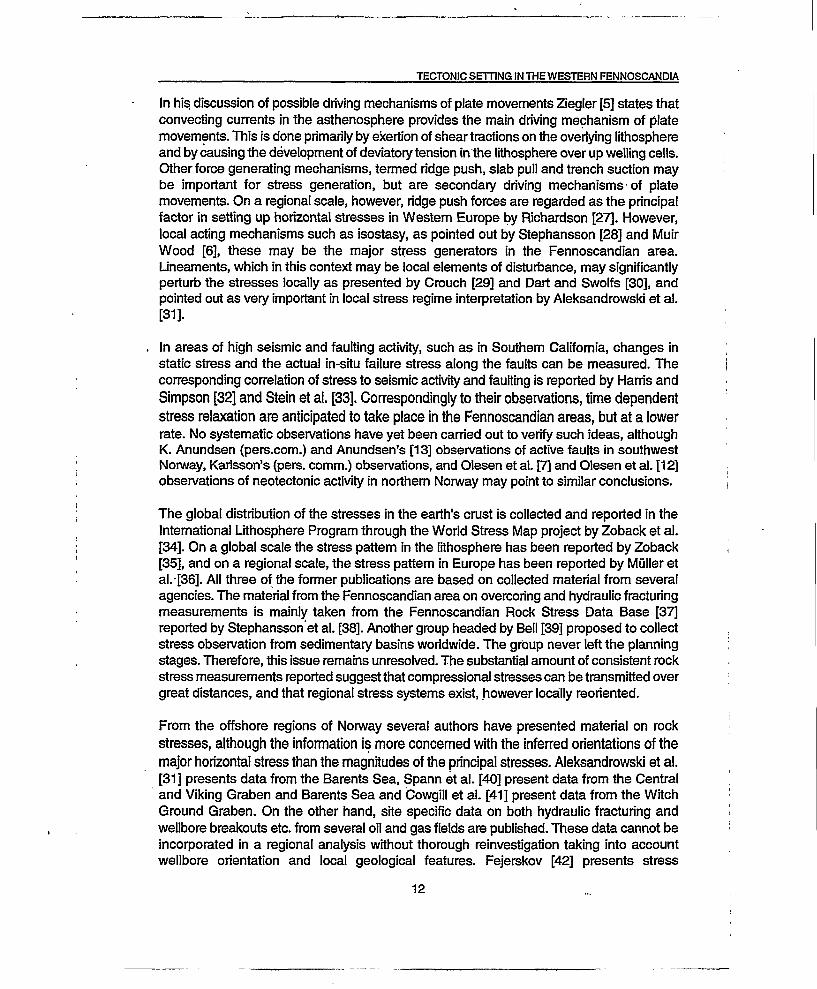
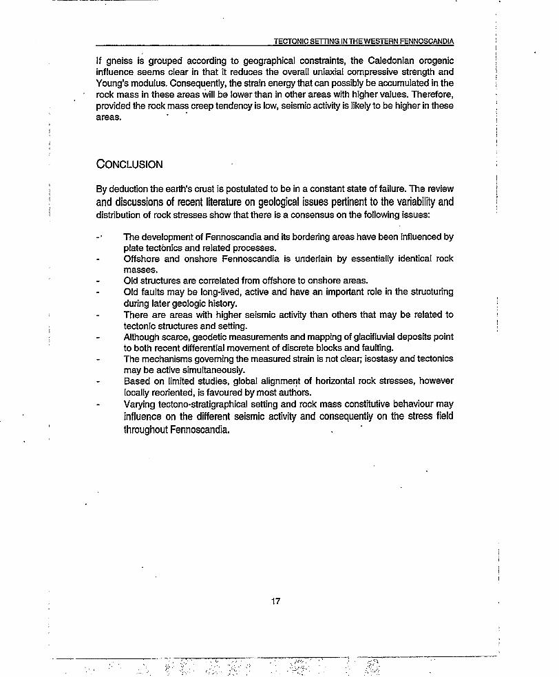
LABORATORY TESTING OF THE NTH cell................................................................................................ 37Determination of the elastic properties........................................................................................37Axial and radial loading of hollow cylinders containing NTH cells........................................ 38Evaluation of the calculated rock stress................................................................................. 46Sensitivity of the NTH cell with respect to grain size............................................................... 54Discussion ....................................................................................................................................... 62Conclusions..................................................................................................................................... 64
QUALITY RANKING OF STRESSES MEASURED BYTHE NTH cell...................................................... 67Evaluation of laboratory test results....................................................................................... 68Evaluation of field measuring results..........................................................................................70Discussions ....................................................................................................................................... 74Conclusions....................................................................................................................................... 75
RECALCULATED ROCK STRESSES AND IMPLICATIONS TO THE REGIONAL STRESS FIELD .... 77Representation of recalculated rock stresses......................................................................... 77Discussion of rock stress measurements................................................................................... 88Conclusions..................................................................................................................................... 93

HYDRAULIC FRACTURING ROCK STRESS MEASUREMENTS................................ 94Equipment for hydraulic fracturing................................................................ "......................... 95Test procedure and interpretation of hydraulic fracturing results................................... 102Casing and cement integrity- formation integrity tests......................................................... 109Assessment of stresses from Leak-off Tests .......................................................................... 120Recommended practice for conducting (Extended) Leak-off Tests...........................■.___ 123Conclusion...................................................................................................................................... 124
MORPHOLOGICAL ROCK STRESS INDICATORS RELATED TO ROCK STRESS MEASUREMENTS ANDTUNNEL SPALLING OBSERVATIONS ........................................................................................ 126Rock stress and rock mechanical properties in the Kobbelv area......................................... 127Spalling observed in the Reinoksvatn headrace tunnel ....................................................... 132Exfoliation observation technique and results........................................................................ 133Discussion ...................................................................................................................................... 135Conclusions.................................................................................................................................... 136
RESULTS FROM SOME STRESS MEASUREMENTS.............................................................................. 138Daleelven................................................................................... 138Fossmark........................................................................................................................................ 139NedreVinstra ................................................................................................................................ 142VlSUND.............................................................................................................................................. 145Discussions .................................................................................................................................... 149Conclusions.................................................................................................................................... 153
FINAL CONCLUSIONS AND RECOMMENDATIONS FOR FUTURE WORK........................................... 155Main conclusions............................................................................................................................ 156Recommendations for improvement of rock stress assessments........................................... 160Recommendations for further work........................................................................................... 162
LIST OF ABBREVIATIONS............................................................................................................. 165
REFERENCES.............................................................................................................................................. 167
APPENDICES 174
Introduction
INTRODUCTION •
General
Evaluation of stress in natural materials has intrigued researchers for several decades, especially since stress has implications to all subsurface activities, and furthermore that stress is a difficult entity to measure. When rock stress is assessed, the setting in which it exists must be addressed. This implies that factors such as the structural setting, the rock mass’ constitutive behaviour, the volume of rock involved and the measuring technique must be considered.
Rock stress as a design tool was accepted as an engineering tool in the early 1960's in Norway according to Li [1]. A decade earlier, permeability measurements were used as a tool for design of injection work related to construction of large underground partly unlined hydroelectric power plants according to R. Selmer-Olsen (pers. comm.). During the 1960's, several research groups worked on the measurement of rock stresses by overcoring according to A. Myrvang (pers. comm.). In the late 1970's researchers started doing hydraulic fracturing to help in the design of the high pressure unlined headrace tunnels of hydroelectric power plants according to J.l. Kollstram (pers. comm.). The loci of this research have been the Norwegian Institute of Technology and the Norwegian Geotechnical Institute. The technological advance’s presented by these organisations would not have been possible without the support and generosity of Norwegian consulting agencies, contractors, mining companies, owners of hydroelectric power plants and petroleum companies.
Rock stress measurements have been conducted throughout most of the Norwegian mainland by both the overcoring and the hydraulic fracturing technique. Focal mechanisms from observations of earthquakes have also been used to assess the principal stress orientation. On the Norwegian continental shelf, stress assessments have been undertaken by conducting pore pressure monitoring, hydraulic fracturing, borehole breakout evaluation, anelastic strain recovery, integrating density logs and evaluating focal mechanisms of earthquakes. Most of these methods are currently in use as means to make prognoses related to the stress gradients and the absolute stress distributions.
1

Introduction
Purpose and method
The purpose of this work is to gain insight in overcoring rock stress measurements using the NTH cell, and to evaluate its ability to convey the stresses acting in natural materials, and furthermore to investigate possible other methods to constrain the stresses. Hydraulic fracturing in particular emerge as a most useful method, not only for evaluation of the minor principal stress from overcoring, but also as a cost-effective technique to assess stresses overall. Because of this versatility, the hydraulic fracturing concept is pursued in both onshore and offshore applications. A second objective with this work is to systematize and investigate if the available measured rock stresses can be used to evaluate the present stress field in the western Fennoscandia.
To evaluate the available overcoring rock stress measurements and to improve the present procedures, a stress calculation methodology is developed. The NTH cells are tested in the laboratory and in-situ overcoring rock stress measurements are conducted; all evaluation is done with this methodology. To investigate the performance of the devised methodology, hydraulic fracturing measurements are conducted using a complete hydraulic fracturing equipment built for this purpose. This equipment is furthermore designed for hydraulic fracturing measurements in shallow ground water wells. Since hydraulic fracturing stress measurements prove successful, their use is also amended and proposed to be used more in petroleum engineering.
The work is intended to contribute to better rock stress measurements in the field. Consequently, easier evaluation of discrete measurement and better evaluation of the whole process of overcoring rock stress measurements are possible. The developed methodology provides the basis for further evaluation of the constitutive behaviour’s effect on the calculated stresses. Combination of different observations and measurements may lead to ambiguities in the actual stresses, but has a positive effect to the understanding of the nature of in-situ stresses in the rock mass.
The developed methodology for overcoring rock stress measurements including the devised code of practise and the constructed equipment for hydraulic fracturing are now in ordinary use at SINTEF. Some equipment has according to needs been further developed.
Thesis organisation
Each chapter,introduces and includes various aspects of rock stress information and techniques, and for the most part they include individual discussions and conclusions. In the text reference is made to several hydro power projects and to some offshore hydrocarbon fields. The different localities are shown in the map in Figure 1.
2

Introduction
TECTONIC SETTING IN THE WESTERN FENNOSCANDIA, gives the global setting and short introduction to the geological history and evolution in the area of interest. Furthermore, some observations of resent stress induced tectonics are pointed to. To the end rock stresses is introduced before the importance of rock mass strength and constitutivebehaviour are emphasized. The chapter concludes with the Earth’s crust possibly being in a state of failure.
TRIAXIAL ROCK STRESS MEASUREMENTS BY OVERCORING USING THE NTH CELL, gives an overview of some methods to evaluate rock stresses, their volumetric dependence and their assessment of rock stress magnitude and orientation. It then presents the overcoring technique as applied with the NTH cell. An improved code of practice for overcoring rock stress measurements is presented, and a new way of calculating the principal stresses is implemented in a computer code incorporating the statistical uncertainty is presented.
LABORATORY TESTING OF THE NTH cell, presents how in-situ elastic properties from retrieved hollow cores with NTH cells are determined, and how the variability involved are assessed. The total sensitivity of the revised overcoring rock stress technique is shown by varying elastic properties, loading conditions and rock grain size. At last, factors affecting the calculated rock stresses are presented.
QUALITY RANKING OF STRESSES MEASURED BY THE NTH CELL, used all available in-situ overcoring stress measurements made with the NTH cell and similar laboratory tests to assess the historical uncertainty involved in the complete stress evaluation. A quality ranking for rock stress measurements by the NTH cell is developed according to the calculated major principal stress and its standard deviation.
RECALCULATED ROCK STRESSES AND IMPLICATIONS TO THE REGIONAL STRESS FIELD, reevaluates all overcoring rock stress measurements with the NTH cell according to the new evaluation methods, and a quality ranking is assigned to each measurement. The results are plotted in maps to show the variability inherent in the measured stresses. The resulting database is subjected to a statistical treatise that suggests a regional grouping of the stress regimes in the western part of the Fennoscandian shield.
HYDRAULIC FRACTURING STRESS MEASUREMENTS, presents ways to find the minor principal stress. A new hydraulic fracturing test rig including packers has been constructed, and is presented with operational and interpretational procedures. The application of the leak-off test in petroleum industry applications is presented with real data from several fields. Based on evaluation of several applications, a recommended practice for conducting (extended) leak-off tests is proposed.
Introduction
MORPHOLOGICAL ROCK STRESS INDICATORS RELATED TO ROCK STRESS MEASUREMENTS AND TUNNEL SPALLING OBSERVATIONS, presents exfoliation mapping as a rock stress indicator in the Kobbelv area, and links the results to overcoring rock stress measurements and tunrtel mapping of spalling. A mapping methodology applicable to other areas as well is presented, where the stress orientation and the stress magnitude compared with the rock mass strength evaluated.
RESULTS FROM SOME STRESS MEASUREMENTS, reports on field measurements in three onshore locations and one offshore location. The measured stresses onshore are related to the discussed rock stress measuring techniques, and the results are compared with other rock stresses measured by overcoring and hydraulic fracturing. The applicability of overcoring and hydraulic fracturing stress measurements are discussed. Using readily available information on stresses from a petroleum well, two possible local stress regimes are discussed.
FINAL CONCLUSIONS AND RECOMMENDATIONS FOR FUTURE WORK, presents a synthesis of the findings and their relevance for rock stress evaluation and improved evaluation techniques, and contains recommendations for future research.
4

Introduction
2° 0°. 2° 4° 6° 8° 10° 1Z» 14° 16° 18° 20° 22° 24° 26° 28° 30° 32° 34'
Figure 1 Location of some of the measuring and observation locations referred to in the text.
5

Introduction
6

TECTONIC SETTING IN THE WESTERN FENNOSCANDIA
TECTONIC SETTING IN THE WESTERN FENNOSCANDIA
Before any attempt to evaluate the present state of stress is begun, the tectono-stratigraphy should be evaluated. Since an emplacement of nappes, faulting and fault zones are the results of stresses exceeding the rock mass strength, these features may be envisioned to cohere with the stress field. Consequently, the present stress field is the result of all processes leading to the current tectono-stratigraphical setting.
The geologic evolution is based on the idea of global tectonic ideas that are generally accepted. The essence of this idea is that the outer shell of the Earth consists of a system of lithospheric plates that move relative to each other over the slowly convecting asthenosphere. These plates are made up of continental and oceanic crustal elements, where oceanic basins are floored by cooled asthenospheric material.
Fennoscandia is the western part of a Precambrian craton overthrusted by nappes of different age and composition during the Caledonian orogeny. To the west, younger sediments represent an almost continuous sequence until the present as shown by Sigmond [2]. Some of these sediments overlay the western part of Norway as shown by Fossen et al. [3]. In the structuring of the North Sea Basin offshore Southwest Norway, Faerseth et al. [4] from seismic and borehole data suggest a clear correlation between both onshore and offshore basement and basement grain, and a structural grain inherited in the younger rocks overlying this. This basement is still active tectonically and consists of a set of separate blocks divided by fracture zones of different type, extent and origin.
Tectonic history and some related observations
The Phanerozoic development of Western and Central Europe may briefly be summed up by the following rendition adapted after Ziegler [5]:
1. Caledonian suturing of Laurussia2. Hercynian suturing of Pangaea3. Permo - Triassic development of Pangaea4. Pangaea breakup: Jurassic-eariy Cretaceous opening of the central and north Atlantic and
western Tethys5. Late Cretaceous and Paleocene breakup of Laurasia and Alpine Collision6. Alpine suturing of Europe and Africa - Opening of Norwegian-Greenland sea7. Later thermal sagging basins with occasional tectonic pulses
7

TECTONIC SETTING IN THE WESTERN FENNOSCANDIA
The post Triassic interplay of the east-west extension on a basement with predefined zones of weakness, reactivated during various stages during the Mesozoic and Tertiary caused the western margin to develop not as a uniform basin, but as a network of interconnected and partly disconnected basins, each with some differences in sedimentation and tectonic history. During the Pleistocene, Fennoscandia experienced several glaciation periods of which the latest ceased some 10.000 years ago. Associated with the deglaciation, reverse faulting is believed to have taken place around 9.000 years BP in the northern Fennoscandia, Muir Wood [6] and Olesen et al. [7] and others. Other types of postglacial faulting have also been reported from several areas in Norway by, e.g. Brekke et al. [8]. Several factors play an active part in the origin of this type of faulting, of which tectonic stresses, glacial rebound, isostasy and material properties are some. Another factor proposed, however speculative, is the shift of the earth's axis of rotation, resulting in faulting coupled to the crust readjusting to the new imposed stress field. Han and Wahr [9] proposed this based on the unbalance imposed due to the melting of the ice caps.
Anda [10] and E. Anda (pers.comm.) identify large scale systems of various sized "blocks" with recent differential semi-vertical displacement in the Romsdal area in the north western part of the Bergen - Namsos gneiss province of Norway, Figure 2. From geometric studies of topographic features, morphology, the elevation and distribution of post-glacial shore lines in the area, Anda [10] suggests differential movements of the blocks to have occurred. His observations show that the differential movements are restricted neither to any rock group nor to any suite of rocks. The nature of this type of observation cannot be determined by observation alone. It must be accompanied by other indications or measurements. K.l. Karisson (pers.comm.) has identified what might be an active fault zone trending NNW - SSE in the highway tunnel between Veblungsnes and Innfjorden close to Innfjorden, in the same area as Anda [10] worked. The deformation has been observed from 1991 to 1993. The continues cracking observed in the concrete tunnel lining may be attributed to identical mechanisms as those governing Anda's [10] observations. These observations therefore confirm the assumptions of the former authors that old structures exist which are still active, and presumably govern the structural style found in younger overlying sediments on- and offshore. Spalling in the roof in the shallow subsea tunnels at the Tjeldbergodden gas processing plant also suggest high subhorizontal stresses, A. Myrvang (pers.comm.). Tjeldbergodden is situated on the northwestern coast of this province within the More - Trondelag - Fault - Zone. The tunnels are oriented perpendicular to the fault zone and the spalling may represent stresses reoriented by the fault zone.
Ahjos and Uski [11] have compiled all known" registrations, on earthquakes in Northern Europe in the period 1375 - 1989. Locations of the recent, and therefore most reliable registrations are centred on and in association to some known lineaments and faults both onshore and offshore. Some onshore features are pointed out by, e.g. Olesen et al. [12] and Anundsen [13]. Major concentrations of earthquakes are associated to the Mid-Atlantic Ridge, and to lineaments such as the More-Trandelag-Fracture-Zone, Jan Mayen Fracture Zone and the southern extension of the Oslo Graben.
8

TECTONIC SETTING IN THE WESTERN FENNOSCANDIA
33 T]eldbergodd(
VEBLUNGSNES
Figure 2 The location of Tjeldbergodden gas processing plant with high stresses in the tunnels and the possible active fault zone in Innfjorden west of Veblungsnes are shown in a segment of the the Norwegian Petroleum Directorate continental shelf map no. 1. In this map known lineaments and faults are plotted. The assumed large scale system of various sized blocks found in the county of More og Romsdal can also be envisioned.
9

TECTONIC SETTING IN THE WESTERN FENNOSCANDIA
Similar observations are found along the coastal zone west of Fennoscandia where the basement has been down faulted to the west as shown in Figure 3 according to Bungum et. al. [14]. Thus, the earthquakes may represent the relaxation of stresses in the earth's crust. However, the origin of the stresses governing this is discussed, although proofs of their existence are found in the thrusting of nappes and earlier faulting that have been active overtime.
Principal structures and lineaments
Several papers have been published concerning both large and small scale structures onshore and offshore Norway, but there does not exist any comprehensive compilation of all this work. Some work on lineaments however, have implications for the development of the structural geology both offshore and onshore Norway as presented by Fserseth et al [4]. Major contributions are presented by Ramberg et al. [15], Gabrielsen and Bamberg [16], Anstad et al. [17], Gabrielsen et al. [18], Rathore and Hospers [19], Lippard and Roberts [20] and Gabrielsen and Fserseth [21]. Brekke et al. [8] have in their compilation of the two- way time map also included the major faults ranging from the Precambrian to the Holocene both offshore and onshore Nonway. Even in this compiled map few of the faults are traced from onshore to offshore environment. However, Stewart et al. [22], Schmidt [23] and Dengoand Rossland [24] show onshore extensions of the regional structural elements that are mapped offshore.
Gabrielsen et al. [25] conclude their structural outline of the Barents Sea region that the major regional fault zones were established in the Carboniferous or earlier. In the subsequent structuring of the region, activity was associated with these elements. The conclusion of others like Rathore and Hospers [19] who have published material on the Southern Norwegian Sea is identical, in emphasizing that the older lineaments are important for the development of later structures.
Distribution of stresses in the earth's crust
Shannon and Naylor [26] state that during various stages of the earth's history, significant portions of the crust are in tension. It appears that when continents are together (the Pangaean or Gondwanaland megacontinents), the interior and marginal areas are often in tension. When the continents are fragmented and spreading, as at present, they are in compression. This is perhaps due to the presence of active spreading ridges in oceanic regions. Convergent pressures affecting the margins of colliding plates may be absorbed completely in the collision zone or may be transmitted in part into the interior of cratonic plates, although juxtaposed along major shear zones. In contrast, divergent pressures do not seem able to propagate stress over such large distances due to the relative low tensional strength of the crust.
10

TECTONIC SETTING IN THE WESTERN FENNOSCANDIA
Figure 3 North Atlantic and Fennoscandian earthquakes and their relation to lineaments and structures presented byBungumetal. [14]. Earthquake locations for the time period 1955 -1989 based on solutions from a variety of reporting agencies, but under requirement that the data from at least eight recording stations be used for each event
11
TECTONIC SETTING IN THE WESTERN FENNOSCANDIA
In his discussion of possible driving mechanisms of plate movements Ziegler [5] states that convecting currents in the asthenosphere provides the main driving mechanism of plate movements. This is done primarily by exertion of shear tractions on the overlying lithosphere and by causing the development of deviatory tension in the lithosphere over up welling cells. Other force generating mechanisms, termed ridge push, slab pull and trench suction may be important for stress generation, but are secondary driving mechanisms of plate movements. On a regional scale, however, ridge push forces are regarded as the principal factor in setting up horizontal stresses in Western Europe by Richardson [27]. However, local acting mechanisms such as isostasy, as pointed out by Stephansson [28] and Muir Wood [6], these may be the major stress generators in the Fennoscandian area. Lineaments, which in this context may be local elements of disturbance, may significantly perturb the stresses locally as presented by Crouch [29] and Dart and Swolfs [30], and pointed out as very important in local stress regime interpretation by Aleksandrowski et al. [31].
In areas of high seismic and faulting activity, such as in Southern California, changes in static stress and the actual in-situ failure stress along the faults can be measured. The corresponding correlation of stress to seismic activity and faulting is reported by Harris and Simpson [32] and Stein et al. [33]. Correspondingly to their observations, time dependent stress relaxation are anticipated to take place in the Fennoscandian areas, but at a lower rate. No systematic observations have yet been carried out to verify such ideas, although K. Anundsen (pers.com.) and Anundsen’s [13] observations of active faults in southwest Norway, Karisson’s (pers. comm.) observations, and Olesen et al. [7] and Olesen et al. [12] observations of neotectonic activity in northern Norway may point to similar conclusions.
The global distribution of the stresses in the earth's crust is collected and reported in the International Lithosphere Program through the World Stress Map project by Zoback et al.[34] . On a global scale the stress pattern in the lithosphere has been reported by Zoback[35] , and on a regional scale, the stress pattern in Europe has been reported by Muller et al. [36]. All three of the former publications are based on collected material from several agencies. The material from the Fennoscandian area on overcoring and hydraulic fracturing measurements is mainly taken from the Fennoscandian Rock Stress Data Base [37] reported by Stephansson et al. [38]. Another group headed by Bell [39] proposed to collect stress observation from sedimentary basins worldwide. The group never left the planning stages. Therefore, this issue remains unresolved. The substantial amount of consistent rock stress measurements reported suggest that compressional stresses can be transmitted over great distances, and that regional stress systems exist, however locally reoriented.
From the offshore regions of Norway several authors have presented material on rock stresses, although the information is more concerned with the inferred orientations of the major horizontal stress than the magnitudes of the principal stresses. Aleksandrowski et al. [31] presents data from the Barents Sea, Spann et al. [40] present data from the Central and Viking Graben and Barents Sea and Cowgill et al. [41] present data from the Witch Ground Graben. On the other hand, site specific data on both hydraulic fracturing and wellbore breakouts etc. from several oil and gas fields are published. These data cannot be incorporated in a regional analysis without thorough reinvestigation taking into account wellbore orientation and local geological features. Fejerskov [42] presents stress
12

TECTONIC SETTING IN THE WESTERN FENNOSCANDIA
orientations on a field - or regional scale from several offshore areas while Golke [43] . presents observations from offshore areas and models stresses along the coast of Norway.
More work of this type from the Central Graben is the Dan field presented by Owens et al. [44] and the Ekofisk area by Teufel and Farrell [45], of which the last authors emphasize the importance of local structures.
The state of stress is determined by the current loading conditions and the stress path defined by the geologic history. In a stable relaxed environment where the rock mass behaves elastic, theoretical vertical (oj and horizontal (oh) gravitational stresses are related to the overburden (h) by equation (1) and (2). In areas with active tectonics, additional stress components may be superimposed on these stresses. At greater depths however, the stresses must equalize because the rock mass cannot sustain unlimited shear stresses. Thus, anisotropic stresses are a surface related phenomenon. If pore pressure (P0) is introduced into the system and the fluids allowed to circulate, the stresses experienced by the rock may be described by the effective stress principle. If there are restrictions to free fluid flow, the poroelastic effect postulated by Biot [46] and further expanded by Biot & Willis [47] by introduction of the Biot factor (a) must be considered. Still in a relaxed environment, the effective theoretical vertical (o‘vt) and horizontal (o"%) stresses are given by equation (3) and (4).
°vt = E Pihi9
1 -v
°'vt = £ P|h,g - ccp0
°ht = 7— °vt " «Po I -V
(1)
(2)
(3)
(4)
where:°v, theoretical vertical stress O'* effective theoretical vertical stressa« theoretical horizontal stress O’h, effective theoretical horizontal stressPo pore pressure a Biot factorg gravitational acceleration P specific weightVI
Poisson's ratio i'th. layer
h overburden
Considering the geologic history of any rock mass as described above, phenomena such as tectonic activity including faulting, isostasy, erosion etc. may have influenced the present stresses and their orientations. These effects would likely have perturbed the stresses
13

TECTONIC SETTING IN THE WESTERN FENNOSCANDIA
locally and regionally. Regarding the stress magnitudes, these effects would furthermore result in additional factors being incorporated in equation (3) and (4).
In crystalline formations comprising fractures, the pore pressure normally increases according to the hydrostatic pressure with depth. In sedimentary basins under extreme conditions, the pore pressure may exceed the minor principal stress causing natural hydraulic fracturing. To sustain any generated overpressure, some sort of sealing mechanism must exist. This could be a low permeability formation in combination with some tectonic activity constraining fluid flow. Several mechanisms for the generation of overpressures have been described although in most situations more than one mechanism is involved. The main processes are considered disequilibrium compaction or undercompaction according to Mann and Mackenzie [48] and Waples [49], while kerogen transformation according to Stainforth [50], and oil cracking according to Barker [51], Spencer [52], Caillet et al. [53]. Other mechanisms such as diagenesis, aquathermal processes and inversion tectonics or overcompaction also play important roles in development and maintenance of high pore pressures. Stress measurements may be misinterpreted if the effect of pore pressure is neglected. This means that to establish correct stress values from measurements, the pore pressure must be evaluated before the final stresses are reported.
The gravitational stresses may be reoriented by topographic or structural features. The measured horizontal stresses are often higher than gravitational stresses would suggest. The additional components differ in magnitude depending on origin, location, lithology, depth and orientation. Parts of the measured high horizontal stresses may be explained by introduction of rock anisotropy in the calculation of the stresses. This is shown by Amadei and Savage [54] and Savage et al. [55], and may represent the normal stress situation. By the introduction of transverse isotropy and subhorizontal layering, the gravitational horizontal stresses increase as the ratio of the horizontal to vertical Young's moduli increase if compared with the linear isotropic elastic case.
Depending on the stress path, stresses may be semipermanent locked in the rock mass. The degree and magnitude of this type of stress will vary according to the individual stress path. Excessive vertical stresses will likely equalize and adapt to a new overburden in shorter time than the horizontal stresses. The release of the horizontal stresses will depend on the viscous properties of the involved rock mass. Generally rocks comprising clay minerals are more susceptible to time dependent stress relaxation than other rocks as discussed in the preceding chapter, excluding halites. On the other hand, stiff elastic rocks may preserve and sustain a high stress level although stress corrosion cracking as explained by Laitaj [56] may be experienced.
DEFORMABILITY OF ROCKS .
Apart from knowledge of the tectonic setting, elastic properties of the host rock are important in evaluation of rock stresses. In recognition of this, rock mechanical test results
14

TECTONIC SETTING IN THE WESTERN FENNOSCANDIA
obtained in the period 1968 to 1991 at SINTEF and NTH were presented by Hanssen et al. [57]. Of the database comprising results from some twenty-seven hundred test samples, more than 50 percent represent gneisses distributed throughout Norway. Due to vague terminology, however, this is a diversified group with inherent variability. In Figure 4 and. Figure 5 where notched box plots1, McGill et al. [58], are used to show the uniaxial compressive strength and the Young’s modulus grouped according to the county of origin, regional trends become visible. The uniaxial compressive strength is lowest for rocks from Nordland and Troms, and may reflect the tectonic impact on rocks found in the Caledonian nappes in these counties. Similar effects may be responsible for the low strength gneisses from Oppland. This is opposite to the relative high strength material in the southern gneiss province comprising the counties Akershus, Hedmark, Oslo, Vest Agder, Aust Agder and Rogaland, and the southwestern gneiss provinces comprising the counties Hordaland, Sogn og Fjordane and More og Romsdal.
Discussion
Although few authors explicitly map the tectonic features from offshore to onshore Fennoscandia, by deduction it is suggested that the lower part consist of identical formations with related structural grain. The upper formations, however, vary regionally according to age and tectonic setting; generally the younger formations are found to the west. The notion of differential movement implies the existence of local stress concentrations and perhaps abnormal and varying vertical stress components. The reported observations on neotectonics prove that post-glacial tectonics has been and still is active in the Fennoscandian area and may lead to anomalous stress magnitudes and orientations. Areas with high tectonic stress levels coincide with the reported seismic activity. In a stable situation, however, the stresses acting in a rock mass are governed by simple physical relationships. Nevertheless, they may be profoundly perturbed by fluid pressures, structural elements, geological processes, tectonic activity, chemical activity and so forth. If the stresses acting in the crust exceed its strength, earthquakes and faulting will take place. The rock mass will go from a higher energy level to a lower through the release of strain energy. The stress levels are thus reduced until a pseudo stable state of equilibrium is accomplished. The magnitude of the measured stresses will therefore be characteristic for the geologic province and the large scale strength characteristics of the rock mass.
1 The notched box plot is an extension of the standard box plot. In this plot the median of the batch
in each group is marked with a vertical line. The lower and upper hinges comprise the edges of the central box. The median splits the ordered batch of observations in half, and the hinges split the remaining halves in half again. The whiskers show the span of observations falling within 1.5 times the absolute difference between the upper and lower hinges and are called the inner fences. The outer fences are defined by three times the same values and divide between outside and far outside values (outliers), shown with asterisks and empty circles respectively. By implementing confidence intervals on the median of groups of observations in a box plot, differentiating between them is possible. A 95 percent degree confidence interval around each median value is shown by notches on the boxes. If these intervals around two medians do not overlap, it is confident at a 95 percent level that the two population medians are different.
15

TECTONIC SETTING IN THE WESTERN FENNOSCANDIA
YOUNGS MODULUS [GPa]
Figure 4 Notched box plots of Youngs modulus for gneiss grouped according to the county where the samples are collected
UNIAXIAL COMPRESSIVE STRENGTH [MPa]
Figure 5 Notched Box plot of uniaxial compressive strength of gneiss grouped according to the county where the samples are collected
16
TECTONIC SETTING IN THE WESTERN FENNOSCANDIA
If gneiss is grouped according to geographical constraints, the Caledonian orogenic influence seems clear in that it reduces the overall uniaxial compressive strength and Young’s modulus. Consequently, the strain energy that can possibly be accumulated in the rock mass in these areas will be lower than in other areas with higher values. Therefore, provided the rock mass creep tendency is low, seismic activity is likely to be higher in these areas.
Conclusion
By deduction the earth's crust is postulated to be in a constant state of failure. The reviewand discussions of recent literature on geological issues pertinent to the variability anddistribution of rock stresses show that there is a consensus on the following issues:
The development of Fennoscandia and its bordering areas have been influenced by plate tectonics and related processes.Offshore and onshore Fennoscandia is underlain by essentially identical rock masses.Old structures are correlated from offshore to onshore areas.Old faults may be long-lived, active and have an important role in the structuring during later geologic history.There are areas with higher seismic activity than others that may be related to tectonic structures and setting.Although scarce, geodetic measurements and mapping of glacifluvial deposits point to both recent differential movement of discrete blocks and faulting.The mechanisms governing the measured strain is not clear; isostasy and tectonics may be active simultaneously.Based on limited studies, global alignment of horizontal rock stresses, however locally reoriented, is favoured by most authors.Varying tectono-stratigraphical setting and rock mass constitutive behaviour may influence on the different seismic activity and consequently on the stress field throughout Fennoscandia.
17

TECTONIC SETTING IN THE WESTERN FENNOSCAND1A
i
ii
18

TRIAXIAL ROCK STRESS MEASUREMENTS BY OVERCORING USING THE NTH CELL
TRIAXIAL ROCK STRESS MEASUREMENTS BY OVERCORINGUSING THE NTH CELL
Rock stress measuring techniques
The state of stress in the rock mass can be assessed in different ways, each method however, offer different advantages and disadvantages with respect to particular applications. One method may give the orientation of one or more of the principal stresses, others give their magnitudes while still others may give the total stress tensor. Also various volumes of the rock mass are affected or involved during testing with different measuring techniques. Furthermore, the various methods have different bases for the stress determination. Table 1 presents a simple grouping of the principal methods of stress determination. The four bases of stress determination apparently represent three length scales extending approximately three orders of magnitude. For results to be comparable implies either a scale-independence of stress state or a knowledge of any scale dependence. Different overcoring measuring practices also assess the stresses in different ways. Stress gradients and absolute stress values have furthermore been shown to vary according to different overcoring methods by Stephansson et al. (op.cit.). This implies that to compare stress values and orientations, proper knowledge of both the test methods and obtainable results must be known before correlations are made.
Table 1 Bases for rock stress determination
Basis Measurement variable
Earthquake Seismic radiationHydraulic fracture Fluid pressureBorehole Geometry of finite deformation, reloading strainsCore Relief strains, evolution of relief strains, reloading strains, finite
deformation state
Table 2 shows the principal results of some various measuring methods. By additional observations, calculations or measurements, the basic results can be augmented and more information extracted. The nature or the origin of the stresses is generally not discemable from the measurements. This must be evaluated based on geological knowledge. Several techniques have been applied to measure the state of stress in the Earth's crust. Some methods have been successfully developed and are in continuos use while others have not been quite so successful and are not in use at all, while still others are in a developing
19

TRIAXIAL ROCK STRESS MEASUREMENTS BY OVERCORING USING THE NTH CELL
phase. Some methods are founded on basic mechanical principles while others use more subtle observed relationships. An overview of some measuring methods is shown in Table3. All methods in this table aim at giving information on the present stresses except the Kaiser effect and the mineral analysis that may also be used to assess paleostresses.
Table 2 Some rock stress measuring techniques and their assessment of orientation and magnitude of the stresses
Rock stress determination method Orientation Magnitude
Flat-jack (#) #Hydraulic fracturing (#) #Overcoring # #Borehole logging # (#)Geological features
# Dnnornol pae>nlt rtf maoonnnn ■
#
iartfi nirnin
(?)
S Principal result of measuring technique(#) Additional measurements are needed for proper determination(?) The method may yield information on this item
Table 3 Some methods available for rock stress determination * I
Overcoring 1D Rigid inclusion
2D Soft inclusion
3D Soft inclusion
Undercoring Borehole slotting Pressurization methods
Indirect methods
Geologic methods
Mast's magnetostrictive cellI rad vibrating wire gage Photoelastic glass / plastic plug USBM cantilever stress gauge CSIR doorstopper strain gage cell CSIR strain gage cell NTH strain gage cell LuH strain gage cell SSPB-Hiltscer deep strain gage cell CSIRO hollow inclusion strain gage cell HBM strain gage undercoring technique Interfels borehole slotting stress meter FiatjackHydraulic fracturingHydraulic testing of preexisting fracturesSleeve fracturingWellbore breakout analysisDifferential strain curve analysisAnelastic strain recoverySonic velocity analysisKaiser effect studiesStructural geologic analysisMineral occurence and orientation analysisEarthquake analysisEvaluation of exfoliation and morphology
20

TRIAXIAL ROCK STRESS MEASUREMENTS BY OVERCORING USING THE NTH CELL
The NTH cell
Triaxial rock stress determination by overcoring was originally presented by Leeman [59]. The method has later been refined and reworked by several organizations, and major contributions have come from the South African Council for Scientific and Industrial Research (CSIR) and the Commonwealth Scientific and Industrial Research Organization (CSIRO) of Australia. The method has been announced as one suggested methods for rock stress determination by the International Society for Rock Mechanics (ISRM) [60]. This presentation will focus on the CSIR version of the overcoring technique.
Myrvang [61] developed a modified version of the CSIR cell, called the NTH cell, shown in Figure 6 (The CSIR cell and NTH cell refer to the triaxial strain cell developed by CSIR and Norges tekniske hogskole (NTH) respectively). The NTH cell has been in regular use since 1969 by the Mining Research Laboratories at the Norwegian Institute of Technology and later by SINTEF Rock and Mineral Engineering. Over the years, the complete state of stress has been measured at more than 200 sites using the NTH cell, all with the objective to solve engineering problems. Thus, some 3000 NTH cells have been used.
The NTH cell body is manufactured of plastics and contains electrical contacts, three strain gauge rosettes spaced at 0°, 90° and 225° around the circumference mounted in compressed air operated pistons. Each rosette has three concentric five millimetres long strain gauges oriented in 0°, 45°, 90° patterns with respect to the cell axis. A passive strain gauge is included in the cell body to form a half bridge. The basic steps involved in the
overcoring technique are shown in Figure 7.
Figure 6 Schematic view of the NTH cell. 1) Strain gauge rosette, plan view. 2) NTH cell, side view. 3) NTH cell, front view showing all three pistons with strain gauges.
21

TRIAXIAL ROCK STRESS MEASUREMENTS BY OVERCORING USING THE NTH CELL
Figure 7 The basic steps involved in triaxial rock stress overcoring measurements. During drilling 76 mm and 36 mm diamond core drill bits are used.1) Drilling to desired measuring depth, 2) Installation of NTH cell, 3) Overcoring the cell.
Factors affecting the overcoring measurements and the stress
DETERMINATION
Due to the nature of the overcoring measuring technique where strain gauges are bonded to rocks, some degree of measurement uncertainty or error is automatically included in the results. These factors can briefly be grouped in three subgroups where the first group is discussed in detail by Hoffmann [62] while the rest is treated in detail by Amadei and Stephansson [63]. The last group is furthermore treated by Myrvang (op.cit.), Amadei [64] and others:
Electrical errors in the measuring chain. Geometric errors in the measuring setup. Assumptions regarding constitutive laws.
22

TRIAXIAL ROCK STRESS MEASUREMENTS BY OVERCORING USING THE NTH CELL
Electrical errors
The'strain measuring chain consists of the active strain gauge, passive completion circuit, power supply, signal amplifier and conditioner, display device and connecting wires. Electrical errors introduced in the measuring chain can significantly reduce the valuable information contained in the measured strain values. The relative change of resistance in an electrical strain gauge is in the order of 10*QJQ. per 10^8. Only minute electrical errors can therefore significantly alter the change of resistance during overcoring, and thus alter the measured strain values. During the evolution of the strain gauge measuring technique effects caused by temperature, signal phase shift, signal loss in lead wires and stability of electrical circuits over time et cetera have been almost eliminated. Measuring stress changes corresponding to ± 1 pS is feasible provided necessary precautions are observed. This group of errors can be significantly reduced by employing a full Wheatstone bridge circuit with 6-wire technology through the complete measuring chain. Experience with overcoring measurements however, show a normal repeatability to be within ± 5 pS.
Geometric errors
Throughout the production of the triaxial measuring cells and the installation equipment, care is taken with respect to alignment and orientation of matching parts. Due to the sliding action of the three pistons which carry the strain gauges, the overall angular orientation error is approximate one degree. If the strain gauges are out of line, the measured strains will be slightly different from nominal values. This may be illustrated if, for example, the principal strain (s) shall be measured by a misaligned strain gauge. The measured strain (s') will be lower, and can be calculated as shown in equation (5). If the misalignment (cp) is five degrees, the reduction in strain will be approximate 1 percent and if the misalignment is one degree, the error will be negligible. This shows that for a proper installation in the present set up of a strain cell, any effect of misalignment is negligible.
s' = -le(1 -cos2q>) (5)
The grid lengths of the strain gauges are five millimetres. The strains, which in the mathematical model are assumed to be measured at an infinitesimal point, are thus averaged over a length of 5 mm. For the axial strain gauges this has no geometric effect. The tangential strain gauges measure the strains over an arc of 8° in the plane perpendicular to the borehole axis, giving a maximal error of 2 percent.
The manufacturers of strain gauges state that when measuring on granular materials, the strain gauge should be chosen to be minimum five times longer than the largest grain to average the strains (Hottinger Baldwin Messtechnik). Only for fine grained rock types will the five millimetres long strain gauges be of sufficient length. For practical purposes however, it seems like the five millimetre strain gauges are an optimum between commercial available strain gauges and maximal length as opposed to the wish for an infinitesimal
23

TRIAXIAL ROCK STRESS MEASUREMENTS BY OVERCORING USING THE NTH CELL
measuring point with respect to the angular accuracy of the measurements. The strain gauges are bonded to the surface of the borehole by two-component bonding cement with short curing time. Under ideal conditions, the cement thickness is approximate 60 pm according to the manufacturer (Hottinger Baldwin Messtechnik), but variations depending on temperature and operator practice occur. This is cared for in the proposed new overcoring measuring procedure presented at the end of this chapter. It is here proposed that Young’s modulus and Poisson’s ratio are calculated from the biaxial modulus chamber tests, giving the apparent moduli, for which the effect of variable cementing practice may be accounted for.
During installation of the NTH cell in the measuring hole, two metre long installation rods with bayonet couplings are used. During another use of the installation rods, severe misalignment was suspected by V.Tokle (pers.comm.). The misalignment was explored, and was systematically increasing as more installation rods were connected. The maximal misalignment angle was more than 20° when 12 installation rods (24 metres long) were connected, or approximately two degrees misalignment per measuring rod. To remedy this, a quicksilver switch was installed in the NTH cell installation head, but was proven unreliable after some testing. The solution has been to install a Schaevitz AccuStar electronic clinometer in the installation head to be able to measure the exact orientation. Thus the orientation of the measuring cell in the borehole is taken care of, and the rotation of the cell is kept within an angular accuracy of one tenth of a degree unaffected by the installation depth.
In overcoring rock stress measurements any misalignment or non-coaxiality of the NTH cells influence the measured strains. Calculation of the stresses however, does not take into account the dimensions or any misalignment of the retrieved core. Nominal bit sizes involved in the overcoring process have outer diameters of 76 mm and 36 mm respectively, that give cylindrical samples with inner diameters of 36 mm and outer diameters of 62 mm. Due to wear, bad drilling practice and different rock types, cores with outer diameters down to 58 mm and inner diameters of up to 39 mm have been encountered. The influence of the core dimensions on the tangential stress concentration on the inner side of a hollow cylinder subjected to only radial loading is shown in Figure 8 when equation 7 is used. The magnitude of the tangential stress in an infinite long hollow cylinder has been determined by Timoshenko and Goodier [65]. Their equation can be rewritten for the tangential stress on the inner surface (ae) when a uniform external pressure (p0) is applied in equation 7.
°e = Po2b2
b2-a2 (6)
where: a Inner radiusoe Tangential inner stress
b Outer radiusPo External pressure
24

TRIAXIAL ROCK STRESS MEASUREMENTS BY OVERCORING USING THE NTH CELL
If the influences of correct geometrical factors are neglected, the error in the tangential stress can be more than 20 percent. Provided Hooke's law is applicable for the material in question, a similar error in Youngs modulus will be made when the biaxial test chamber is used for elastic properties determination. An error in the estimate of Poisson’s ratio is also introduced simultaneously. If the necessary precautions are taken while drilling, this will not cause any problems.
□ 1,1-1,2;
iQ 0,9-1 ,
INNER DIMENSION [mm]
OUTER DIMENSION [mm]
Figure 8 The influence of inner- and outer dimensions of the hollow core on the magnitude of the measured tangential stresses during overcoring stress measurements shown as the stress concentration factor. In extreme cases where problems during coring operations are encountered, measured stresses can be overestimated by a factor of more than 1.2.
Furthermore, if the applied external pressure to a hollow core containing a NTH cell shall mimic the far-field stress (a,), it must be corrected for geometric effects related to being applied only a small distance from the measuring cell. This is shown in equation (7) and is applicable when the biaxial test is used to evaluate the NTH cell.
po = °i (1" 5 (7)
where: o. Stress at infinity p0 External pressurea Inner radius b Outer radius
25

TRIAXIAL ROCK STRESS MEASUREMENTS BY OVERCORING USING THE NTH CELL
Elastic parameter influence
The cores retrieved in overcoring rock stress measurements have been used as the standard laboratory core size at NTH and SINTEF. The sonic velocity, bulk density, unconfined compressive strength, failure angle, Youngs Modulus and Poisson's Ratio are therefore determined using solid cores with a diameter of 62 mm and a 2,5:1 length to diameter ratio. Rock tensile strength is estimated by the Point Load Index, using cores with a diameter of 22 mm.
The stress calculation is based on Hooke’s law for a linear elastic isotropic media, which means that only Young’s modulus and Poisson’s ratio are needed. Errors in the determination of these two constants subsequently result in wrong stress values. Youngs modulus is determined as the initial secant modulus during loading and Poisson’s ratio is determined similarly. Any nonlinear behaviour during initial loading of the sample is neglected in the calculation. The testing may consequently give lower estimates of the elastic properties than expected. This could be overcome by applying the tangent modulus at a uniaxial stress of o = 20 MPa. The mechanism of overcoring is however unloading in nature, and therefore it would be appropriate to use the unloading tangent modulus instead.
The elastic constants may be determined in three different ways. Solid cores next to the measuring cells can be loaded in uniaxial compression and the elastic constants can be calculated. The hollow cores containing the overcored triaxiai cells may also be tested in uniaxial compression and thus give the elastic constants. The third possibility is to load the hollow cores containing the overcored triaxiai cells radially in a biaxial modulus chamber and calculate the elastic constants. The first two test methods must be conducted in the laboratory because preparation of the end surfaces is needed. The biaxial modulus chamber can be used in the field, and provides a unique way to both test the functionality of the newly overcored cells and to decide the elastic properties of the rock. The equipment and test procedure is described by Fitzpatric [66].
Table 4 Comparison between elastic properties on some rock types obtained from tests on solid 62 mm diameter cores and hollow overcored NTH cells subjected to axial compression.
Average values, Average values,solid core (LVDT) hollow core (NTH cell)
Site Rock type E [GPa] V E [GPa] V
Fossmark hydropower station Gneiss 38.3 0.12 48.6 0.14Moflat hydropower station Metarhyolite 20.9 0.14 28.5 -Mar hydropower station Metarhyolite 34.3 0.19 45.7 0.26Vinstra hydropower station Sandstone 33.1 0.29 62.1 0.31
Elastic parameters determined from tests on hollow cores containing NTH cells and solid 62 mm diameter cores with external LVDT (linear variable displacement transducer) instrumentation are shown in Table 4. All tests show that both Young's modulus and
26

TRIAX1AL ROCK STRESS MEASUREMENTS BY OVERCORING USING THE NTH CELL
Poisson’s ratio is lower when solid 62 mm samples are tested. The degree of underestimation varies from at maximum approximately 50 percent to almost nil. When elastic properties obtained on solid 62 mm diameter cores are used in stress calculations, the in-situ stresses are underestimated. However, the degree of underestimation may vary. This is caused by the volumetric strength relation.
The recommended ISRM method2 to calculate the elastic parameters is to use stress and strain values in uniaxial compression between 40 percent and 60 percent of the maximum axial stress at failure. This procedure has not been followed in the testing described above, and is seldom met in any of the material tests related to overcoring rock stress measurement presented or referred in this work. If however, the sample shows irreversible behaviour in successive loading steps, the recommended ISRM method to decide the elastic properties may not be adequate for a proper description. Instead of this test method, the sample may be subjected to cyclic increasing axial stress similar to what is shown in uniaxial tension by Okubo and Fukui [67]. Thus, the visco - plastic part of the strain may be eliminated. By that, the unloading and/or reloading paths are used to find the pure elastic properties of the sample. Examples of these test types are shown in Figure 9 to Figure 12. Two different gneiss samples with diameters of 62 mm have been tested in uniaxial compression. The axial strain is measured by two clamp-on extensometers spanning 51 mm while the radial strain is measured by a circumferential extensometer. The first gneiss sample show loading - unloading tangents that suggest stiffer pure elastic response than the initial loading path. The second gneiss sample responds almost in a linear elastic manner, but some hysteresis and non-linearity are evident.
Residual stress influence
Normally, stresses are treated as tractions. Therefore, no allowance is made for any irreversible change of internal forces. Lejon [68] and Hiltscher et al. [69] report residual stresses from overcoring experiments in traction free excavated rock blocks and boulders. Residual rock stress up to 5 MPa and 15 MPa are measured by the authors respectively, comparable with in-situ stress magnitudes less than 30 MPa. Similar relationships have also been reported by Buen [70] and Myrvang [71] in a rock block excavated northwest of the Trondheim area.
2 International Society for Rock Mechanics: "Suggested methods for determining the uniaxial compressive strength and deformability of rock materials".
27

TRIAXIAL ROCK STRESS MEASUREMENTS BY OVERCORING USING THE NTH CELL
Figure 9 Loading history of 62 mm diameter sample of gneiss. See also stress strain behaviour below.
-2.000 -1.750 -1.500 -1.250 -1.000 -0.750 -0.500 -0250 0.000 0.500 0.750
Strain [mS train]
Figure 10 Stress strain plot showing hysteresis through the cycling loops of the gneiss. Onset of dilatancy and uniaxial compressive strength are identified in the axial stress - strain graph to the right in the graph. See also loading history above.
28

TRIAXIAL ROCK STRESS MEASUREMENTS BY OVERCORING USING THE NTH CELL
----------------------------------------------------------------------------------------------------------------------------------------------------------------------------------------------------------------------------------------------------------------------------------------------------------- ?
Figure 11 Loading history of 62 mm diameter sample of gneiss. See also stress strain behaviour below.
rii
•0.100 0.000 0.050 0.100 0.300•0.150
Strain [mStralnJ f
Figure 12 Stress strain plot showing almost no hysteresis through the cycling loops of the gneiss. See also loading history above.
29

TRIAXIAL ROCK STRESS MEASUREMENTS BY OVERCORING USING THE NTH CELL
Revised measuring and evaluation methods for overcoring
MEASUREMENTS USING THE NTH CELL
When overcoring rock stress measurements were first undertaken, the objective was better tunnel, stope or pillar design, i.e. optimization of load bearing capacity of the rock mass was the objective and the major stress was of prime interest. This implies that large stresses were of major concern. Later, the focus shifted to design of the immediate roof of near-to- surface public halls or the waterways of hydroelectric power plants, i.e. calling for precise measurement of small stresses or the minor principal rock stress. After this shift of focus, the accuracy of the overcoring stress measuring technique has been questioned. Furthermore, the designers of subsurface structures have been forced to include rock mechanics and stress analysis as a design tool to document the engineering basis for a chosen solution. Therefore, growing needs for both measuring and calculating rock stresses, its redistribution and the associated confidence intervals have emerged. Based on experience gained through practical rock stress measurements and evaluation of engineering or geological problems during the period 1982 to 1990, a revised overcoring measuring procedure and a new evaluation method are proposed. It is based on the need for better assessment of the uncertainty related to the calculated stresses, SINTEF's practice for overcoring and Myrvang's (op.cit.) solution of the Kirsch equations.
Other authors use various techniques to solve the stresses from the measured strains. Leijon [72] has devised a 12-strain gauge cell (the LuT Cell), and uses the redundancy in the strain readings to employ a least square technique when calculating the stresses at each measurement point. Walker et al. [73] on the other hand calculate the stress tensor for each measurement point and then applies a Monte Carlo simulation technique to assess the statistical confidence intervals for all the rock stress measurements. Parallel to thepresent work Jupe [74] has presented a statistical method to evaluate rock stress measurements. He has used a Jackknife resampling technique originally presented by Effron [75] to assess the statistical uncertainties involved in the measurements. Snider et al. [76] have published a checklist type of work programme for overcoring stress measurements. Although this is meaningful for measuring crews using their dedicated equipment, it will only be of limited use for others.
To profit from both portable computers and testing equipment, the measuring crew should consist of three persons. Two persons should do the diamond drilling and take overcoring measurements while the third person tests the retrieved cores and calculates the complete stress state. Alternatively, the measuring crew may consist of only two persons as is common practice today at SINTEF. There will, however, be a tradeoff in time in preference for the first instead of the second crew plan. Since both material testing and stress calculation are new to the current set up, it will increase the time spent at the measurement site. The ultimate set up will therefore be to use a three-man team on large or time-critical jobs, and use the standard two man teams for regular jobs. The objective however, must be to focus on quality workmanship in the complete overcoring stress measuring chain, from planning through measuring to reporting. The new procedure using the NTH cell presented in Table 5 is designed to meet this objective.
30

TRIAXIAL ROCK STRESS MEASUREMENTS BY OVERCORING USING THE NTH CELL
When triaxial rock stress measurements are conducted to assess the global state of stress, identification of both magnitude and orientation of the stresses are sought. This information should in addition incorporate all measuring uncertainty and give the confidence limits for the entire measuring and calculation process, enabling a complete appreciation of the state of stress and the uncertainty involved in attaining it. Following these conditions, the new evaluation method is formulated and shown in Table 6. In the calculations, all measurements are pooled and six different strains with values for Young’s modulus and Poissons ratio are chosen at random. The resulting stresses are calculated and stored. Aftera sufficient number of calculations, the mean principal stresses and orientations are calculated with their standard deviations and can be presented as distribution curves.
The core features of the resulting computer code are shown in Table 7. The actual numerical programming has been contracted to Ming Lu, who presented the results in two reports, Lu [77] and Lu [78], and named it DISO (Determination of In-situ Stress by Overcoring). The input data to the computer code is repeated in the output file with the calculated stresses and their orientation, as shown in Table 8. The computer code has been further developed based on the original concept. A new version includes simultaneous calculation of stresses from 2D and 3D overcoring measurements from one borehole since it is normal practice to do 2D overcoring measurements if poor measuring conditions are encountered during triaxial overcoring measurements.
In order to exclude outlying strain values, the streamlining factor is introduced. The streamlining factor is the maximal relative standard deviation for the calculated principal stress accepted during the final calculation. If a chosen set of strains leads to calculated principal stresses deviating more than the range given by the streamlining factor (some part of the standard deviation given by the operator), these results are omitted during a second calculation of the mean principal stresses.
Discussion
Rock stress measurements by overcoring using the NTH cell have proven their value through measurements under various conditions through the last three decades. There are still potential for enhancements coupled to the overcoring rock stress measurement process. To assess possible enhancements, the complete process must be considered, from location of measuring sites to evaluation of the calculated stresses. Before the various enhancements are conceived, a way to evaluate their possible effect is needed. This is done by creating a statistical approach to the evaluation of the calculated principal stresses, which has been implemented in the computer code DISO. By using this, the effect of changing any part of the complete overcoring process can be assessed, i.e. any change’s effect on the mean stresses and their standard deviation can be seen and compared with the cost involved.
31

TRIAX1AL ROCK STRESS MEASUREMENTS BY OVERCORING USING THE NTH CELL
Table 5 Revised procedure for rock stress measurements using the NTH cell, where item 12 to 14 represent the proposed improvement to the present code of practice-
1. ' Drilling of the measurement hole into the rock mass to the point where the stresses are to bemeasured. Drilling bit size is 76 mm diameter, giving cores with 62 mm diameter.
2. Flattening the end of the hole with a facing drill bit.3. Drilling of a concentric borehole approximate 25 cm further into the rock mass, with bit size of
36 mm diameter, giving cores with 22 mm diameter.4. Inspection of 22 mm cores to find the placement of the measuring cell, ensuring no fractures
or lithology change nearby.5. Flushing and drying of the measuring area in the hole.6. Installation of the measuring cell, including orienting and cementing.7. Taking initial readings of strain gauges.'8. Overcoring of measuring cell and drilling totally 50 cm, which also gives undisturbed rock core
fortesting purposes.9. Measuring of post-overcoring strains for each strain gauge.10. Calculation of strain relief values by subtracting initial from post-overcoring strain values.11. Measuring the borehole orientation.12. Determination of elastic moduli and functionality of the overcored measuring cell by use of the
biaxial modulus chamber. ,13. Calculation of principal stresses and their orientation for each overcored measuring cell.14. Evaluation of results and decision whether to do more measurements.15. Laboratory determination of mechanical and elastic properties on 62 mm cores.16. Evaluation of results with respect to the engineering question to be solved.
Table 6 New procedure for calculation of stresses from measured strains measured by the NTH cell. !i
1 Setting up the measured data and site specific parameters (borehole orientation, measured !strains, elastic parameters, vertical overburden, average rock density). i
2 Random selecting a set of different strains and elastic parameters from the above matrix. j3 Calculation of the stress tensor, the resulting principal stresses and their orientation. |4 Repetition of step 2 and 3 a sufficient number of times to ensure the calculation of the
confidence limits with statistical certainty.5 Calculation of the mean values and standard deviations for the stresses assuming normal
distributions.6 Evaluation of the standard deviations for the stresses in order to detect measured strain
outliers (erroneous measurements).7 Recalculation of the stresses omitting strain outliers.8 Calculation of the vertical stress component, and the major- and minor horizontal stresses ■
with their respective bearings. ,9 Calculation of the theoretical gravitational stresses. !10 Plotting the distribution of the magnitude of the stresses. * 1 1111 Plotting the mean values and selected confidence limits in stereographic projection.12 Evaluating the stresses and their orientation considering theoretical gravitational stresses, I
rock mass structure and topography.
32

TRIAXIAL ROCK STRESS MEASUREMENTS BY OVERCORING USING THE NTH CELL
Table 7 Calculation steps of the computer code DISO ver. 2.1
1 Preparation of input database2 Random selection of a set of nine differently oriented strains and elastic properties.3 Storage of the calculated 36 real stress solutions.4 Repetition of point 2 and 3 until more than 20.000 or a predetermined number of complete
datasets are stored.5 Calculation of the statistical parameters from the database.6 Detection of outlying strain values from the measurement database based on a
predetermined relative standard deviation of the calculated stresses (streamlining factor).7 Recalculation of the stresses omitting detected strains causing stress outliers.
Table 8 Output file from the computer code DISO ver.2.1 showing both input values and calculated results for three dimentional rocks stress measurements
IN SITU STRESS MEASUREMENT REPORTClient Name: NEDRE VINSTRABorehole Name: VINS01Borehole orientation: Trend 37.0 Overburden: 265.0 m
Project Name: NEDRE VINSTRA Report Number VINS01 Elevation angle 5.0
MEASUREMENT RESULTDEPTH 3-D READINGS 2-D READINGS
C* P /> C* C> n £> A rt pt p11 zV'le, e2 e3 ®4 ®S ®6 ®7 ®8 ®9 e' e" e'" e"" E V
6.0 -20 30170 -60680415 -35 525190 0 0 0 0 59.0 0.21 27606.5 30 485 240 90 305 225 -85 460 95 0 0 0 0 59.0 0.21 27607.3 -5 805720 -15 185 85 -20 195 -90 O 0 O 0 59.0 0.21 27607.8 35115180 35 405 210 -35 -100-35 0 0 0 0 59.0 0.21 27608.3 5 153 290 95 415 275 20 260 -15 0 0 0 0 59.0 0.21 27608.8 65 60 210 -40 695 240 45 205 130 0 0 0 0 59.0 0.21 2760
STATISTICAL RESULTS OF IN SITU STRESSESMEAN AV.DEVST.DEV TREND PLUNGE
SIGMA1 13.43 3.49 4.16 317.3 23.7SIGMA2 9.77 1.77 2.08 72.2 43.8SIGMAS 4.36 2.37 2.73 208.1 36.9
IN SITU STRESSES IN VERTICAL AND HORIZONTAL DIRECTIONSMAGNITUDE ORIENTATION
VERTICAL STRESS 8.41MINIMUM HORIZONTAL STRESS 6.49 37.1MAXIMUM HORIZONTAL STRESS 12.66 127.1
GRAVITY STRESSVERTICAL STRESS: 7.17 HORIZONTAL STRESS: 1.91
33

TRIAXJAL ROCK STRESS MEASUREMENTS BY OVERCORING USING THE NTH CELL
After the introduction of the current enhancements; the biaxial chamber to find the elastic properties and a new calculation procedure to calculate the stresses, the next items in the measuring chain to be optimized should be the electrical system. Wire configurations (six- wire versus standard wiring systems), strain gauge completion circuit (full bridge versus half bridge in the measuring cell), connectors and continuous readout of strains during overcoring are the logical way to do this. The constitutive model employed in the calculation should also be subjected to scrutiny. A linear elastic isotropic model may not be the optimum for all rock types involved. The best way to consider which constitutive model to apply in the future, is to develop interpretation software for the biaxial test chamber and evaluate restressing experiments of overcored NTH cells. After that, the path should be clear for implementation of possible new constitutive models for the improved stress calculations. In this context the method described by Amadei and Stephansson [63] for analysing stresses in anisotropic rocks may be employed in the devised calculation scheme incorporated in the DISC computer code.
~ t|
Conclusion jTo assess the state of stress, actual measurements must be conducted. Several methods have proven their worth under various circumstances. Some methods are better for certain applications than others because they imitate or represent physical processes that are characteristic for the question to be solved. In the preceding tables, different methods of !stress measuring techniques, their bases and their assessment of the full stress tensor are shown.
The NTH cell has successfully been used for overcoring stress measurements through the last three decades. When the chain of operations involved are viewed as a whole, it is now possible to optimize each individual subactivity in a cost-efficient way. To do this, a computer program has been developed to assess the statistical variation of the calculated stresses. Thus, the effect of all processes leading up to the final stresses can be evaluated.This methodology will also be suitable for further improvements of the NTH cell overcoring method in the future.
During the process of reviewing the overall performance of the NTH cell in field and laboratory applications, some improvements have been accomplished and some more are proposed. An orientation tool has been mounted in the installation head to reduce systematic errors in orientation of the NTH cell. In the practical use of the overcoring method a revised code of practice is proposed which includes use of the biaxial test chamber for evaluation of the elastic parameters. This should be applied at the measuring site to guide in the on-site assessment of the measurements. An increase of as much as 50 percent in Youngs modulus is shown from tests conducted on overcored rock cylinders containing
34

TBIAX1AL ROCK STRESS MEASUREMENTS BY OVERCOMING USING THE NTH CELL
NTH cells as opposed to tests on standard solid cores. The common practise of using solid cores should therefore be stopped and changed to the use of overcored hollow cylinders containg NTH cells. The evaluation of geometric influences show that improper core drilling may affect the results significantly. Up to 20 percent variations from nominal values are shown. Under unfavourable measuring conditions this may totally ruin what would otherwise be termed medium results.
Other parts in the measuring chain that may be optimized are the use of six-wire electrical connected full bridge strain gauges which are computer-monitored during overcoring, and investigation into other constitutive models.
35

TRIAXIALROCK STRESS MEASUREMENTS BY OVERCORING USING THE NTH CELL
36

LABORATORY TESTING OF THE NTH CELL
LABORATORY TESTING OF THE NTH cell
To test the function of the NTH cell, and by that its performance and applicability to measure in-situ stresses, several laboratory experiments have been done. The NTH cell's ability to reproduce the strain caused by loading mechanically uniform and stable materials have been investigated in the laboratory by loading hollow aluminum and steel cylinders while recording the resulting strains. Its ability to predict the in-situ elastic constants is also tested by similar tests. In addition three igneous rock types with varying grain size have been used • to evaluate possible adverse effects. The computer code DISC has been employed to evaluate the repeatability and uncertainties involved in 'doing several rock stressmeasurements for all material types. In the previous chapter the constitutive, geometric and electric factors have been discussed, and will only briefly be touched upon here.
Determination of the elastic properties
The two elastic constants, Youngs modulus (E) and Poisson’s ratio (v), are calculated using the averaged axial (ea) and circumferential (§) strains measured by each strain gauge
rosette in the NTH cell. This can be done because it is assumed that the test specimens are homogeneous, linear elastic and isotropic. Then the average elastic constants are calculated and used in the later calculation of the stresses. The averaging process eliminates any effect of non-coaxial loading for the axial tests and reduces the error bandwidth for all test series. The applied stress is taken as the reference stress in the calculations. For the metal tests a set of real and nominal elastic constants are calculated from the measured strains and applied stresses.
In uniaxial compression when the stress distribution in the hollow cylinders is uniform, the elastic constants may be calculated using Hooke's law and the definition of Poisson’s ratio. This is done for both cylindric solid and hollow specimens and is shown in equation (8) and ■ (9). The starting secant moduli are calculated. When hollow cylinders are subjected to radial stresses in the biaxial modulus chamber, the radial stresses through the hollow cylinders are non-uniform and must be accounted for in subsequent calculations.This is seen in the geometric factor in equation (10). Small tensile stresses" are also induced axially during radial loading in the tested cylinders. In the mid-section of the uniformly loaded hollow core however, the strains are very similar to the strains in an infinite loaded hollow core, and no correction is required to calculate the "real" elastic constants according to Worotnicki [79]. If the strain gauges were placed close to the ends of the hollow cylinder, the strain readings would have been misinterpreted. The elastic properties derived from hollow cylinders and used in calculating the principal stresses, are given by equation (10) and (11) respectively.
37

LABORATORYTESTING OFTHE NTH CELL
For both the metal - and the rock samples, the initial secant elastic moduli during loading are calculated.
= °a Z ea (8)
~ E0 / sa (9)
2p0b2(10)(b2-a2)Sg
- ea / s6 (11)
where: E: Youngs modulusoa: Axial stress in test cylinderea: Axial straina: Inner radius of a hollow core
v: Poisson’s ratio p0: Applied external pressure ee: Circumferential strain b: Outer radius of a hollow core
Axial and radial loading of hollow cylinders containing NTH
CELLS
NTH cells were mounted in hollow cylinders of aluminum and mild steel manufactured by use of a turning lathe to let them resemble overcored rock cores. The nominal material properties of the metals are shown in Table 9. Assembly of the NTH cells in the hollow cylinders was done by SINTEF's skilled measuring crew to ensure conditions similar to those experienced in the field. The assembly took place under stable environmental conditions in the laboratory ensuring optimal performance of the total measuring chain. The test programme consisted of initial axial loading of the hollow cylinders with NTH cells in a hydraulic testing machine, i.e. a Losenhausen 100 kN load frame. After that, the samples were loaded radially in a biaxial modulus chamber borrowed from Renco AB of Lulea. The loading was increased gradually and the stresses and the resulting strains were measured for each load step. Under biaxial loading, the circumferential stresses on the inner side of the hollow cylinder are higher than shown in the figures. In these figures the strains are plotted versus the applied stresses on the outer surface of the hollow cylinder. Examples of stress versus strain curves are shown in Figure 13 for axial and radial loading of steel cylinders respectively. In the figures, the measured, averaged and theoretical strains are shown for a hollow metal cylinder under axial and radial loading. During the loading tests,
38

LABORATORY TESTING OF THE NTH CELL
a set of measured strains were collected and compared with the theoretical strains calculated from the applied stress and the nominal elastic properties.
To evaluate the two ways of determining the elastic properties, axial - and radial loading, the averaged measured axial and circumferential strains from each cell were evaluated by the calculations. The reason for doing so was that non-coaxial loading occurred during axial tests. When the three axial or circumferential strains of the NTH cell are averaged, any effect of non - coaxial loading is eliminated. If the test setup was perfect during the axial loading, the measured axial, circumferential and oblique oriented strain for the three strain gauge rosettes should have given identical results respectively. As shown in Figure 13, this was not observed. Strain readings that should have been almost identical differed considerably, especially for the axial tests. The most likely reason for this was unparallel end surfaces of the hollow cores. The skewness of the end surfaces was later measured to be in the order of 1/20 mm. Although spherical heads were used in the load frame, bending and thus moments were introduced in the sample. These irregular results could also be caused by non-coaxially loading in the load frame used in the tests. The axial loading test method was therefore regarded to be an unsuitable technique for testing or controlling the NTH cells unless special precautions were applied. This suggests that spherical seats in the testing machine do not provide a remedy for bad specimen preparation. However, almost identical results were obtained using the averaged strains from the three strain gauge rosettes when Youngs moduli and Poisson’s ratios were calculated.
A summary of the results from both axial and biaxial testing of hollow metal cylinders installed with NTH cells is shown in Table 10. All measured strains during radial and axial loading is given in tables in the appendix. In Table 10 median values and relative errors of measured strains and calculated elastic constants are shown versus applied axial or radial stress. These results are based on strain measurements for four to eight single strain measurements. The median strain values are shown graphically in Figure 14 to Figure 29 with the absolute strain measurements from each cell. The nominal or theoretical strains calculated from the actual stress and the elastic constants are also shown in the figures. Youngs moduli and Poisson’s ratios are also calculated and shown in Table 10 and Figure 14 to Figure 29.
39

LABORATORY TESTING OFTHE NTH CELL
Table 9 Nominal elastic properties of steel andaluminim test materials
Material type Youngs modulus [GPa] Poissons ratio
210 0,30Mild steel Aluminum 6082 69 0,33
-400 -200 800 1000Meesurod strain [micros]Strains on Inner surface [micros]
Figure 13 Strains measured by all nine strain gauges of the NTH cell during radial loading of the aluminum cylinder no.4.1 to the left and axial loading of the aluminum cylinder no.1.1 to the right The experimental strains are shown by box symbols for radial (circumferential) strains, diamond symbols for 45° strains and triangle symbols for axial strains. Average strains in all three strain gauge directions are shown by solid lines and theoretical strains are shown by dashed lines. All stresses are refered to the outer surface, while strains are measured on the inner surfaces.
40

LABORATORY-TESTING OFTHE NTH CELL
Table 10 Results from axial and radial loading of hollow steel and aluminum cylinders containing triaxial NTH cells (All strains are median values).- In the test column, -a represent axial loading and -r represent radial loading for steel and aluminum samples. These results are also shown graphically in Figure 14 to Figure 29.
Test o s. Sat As. Ea Sa ASg E AE v Av NMPa gS MS % MS MS % GPa % % #obs
Steel-a 2.3 9.3 10.9 -14 -3.2 -3.1 3 244.9 17 0.297 -10 8Steel-a 4.6 20.3 21.7 -6 -6.3 -6.7 -6 224.7 7 0.297 -10 8Steel-a 9.1 42.5 43.5 -2 -12.5 -14.0 -11 214.8 2 0.289 -12 8Steel-a 13.7 64.2 65.2 -2 -19.3 -21.2 -9 213.5 2 0.298 -10 8Steel-a 18.3 86.2 86.9 -1 -25.0 -28.4 -12 211.9 1 0.289 -13 8Steel-a 22.8 108.3 108.7 0 -31.5 -35.8 -12 210.7 0 0.288 -13 8Alum-a 2.7 34.0 39.3 -13 -10.0 -13.0 -23 79.7 16 0.294 -11 6Alum-a 5.4 67.5 78.6 -14 -20.5 -25.9 -21 80.3 16 0.304 -8 6Alum-a 10.8 136.5 157.1 -13 -42.0 -51.9 -19 79.4 15 0.308 -7 6Alum-a 16.3 206.0 235.7 -13 -64.0 -77.8 -18 78.9 14 0.311 -6 6Alum-a 21.7 278.5 314.3 -11 -86.5 -103.7 -17 77.9 13 0.311 -6 6Alum-a 27.1 351.0 392.8 -11 -109.0 -129.6 -16 772 12 0.311 -6 6Steel-r 3.2 -13.5 -15.0 -10 47.0 46.0 2 205.4 -2 0287 -13 6Steel-r 8.2 -35.0 -39.0 -10 118.0 117.8 0 209.7 0 0297 -10 6Steel-r 13.2 -58.0 -62.0 -6 192.0 189.7 1 207.4 -1 0.302 -8 6Steel-r 18.2 -80.5 -86.0 -6 264.0 261.5 1 208.0 -1 0.305 -8 6Steel-r 23.2 -102.0 -110.0 -7 334.5 333.3 0 209.3 0 0.305 -8 6Steel-r 28.2 -124.5 -134.0 -7 405.0 405.2 0 210.1 0 0.307 -7 6Alum-r 3.2 -54.5 -47.8 14 141.5 144.9 -2 70.7 2 0.385 17 8Alum-r 8.2 -131.0 -122.6 7 348.0 371.4 -6 73.6 7 0.379 15 8Alum-r 13.2 -212.0 -197.3 7 564.0 597.8 -6 73.1 6 0.378 15 7Alum-r 18.2 -281.5 -272.0 3 769.0 824.3 -7 74.0 7 0.361 9 4
a - External stress sa- Axial measured strainsa, - Theoretical axial strain Aea - Relative difference between sa and s*s8 -Circumferential measured strain e% - Theoretical circumferential strainASg - Relative difference between Sg and e& E - Experimental Youngs modulusAE -Relative error between nominal and experimental E v - Experimental Poisson ratioAv - Relative error between nominal and experimental v N - Number of tests
41
LABORATORYTESTING OFTHE NTH CELL
15 •
•Edrcmed
+ Edrc
Strain on inner surface of holow cylinder [mkroS]
Figure 14 Theoretical, measured, and median strain values for axially loades steel cylinders containing NTH Cells
Eax%Edrc%
Axial stress in hoHow cylinder (MPa)
figure 15 Average relative error in measured axial and circumferential strains in hollow steel cylinders under axial loading
•0.9
••0.8
■0.7± + + +......f......t—$
•05150 •• -0.4
100
Axioi stress in hollow cyfinder [MPa)
Figure 16 Theoretical, measured and median Youngs modulus and Poisson's ratio calculated
from measured strains in hollow steel cylinders under axial loading
-10 • •
Axial stress in hollow cylinder (MPa)
Figure 17 Average relative error in calculated Youngs modulus and Poisson's ratio calculated from measured strains in hollow steel cylinders under axial loading
42

LABORATORYTESTING OFTHE NTH CELL
-200 -100Strain on Inner surface of ho Bow cySnder
[micros]
Figure 18 Theoretical, measured, and median strain values for radially loaded steel cylinders containing NTH Cells
mi mi
250-
200-
150-
100-
Radial stress In hollow cylinder (MPa)
Figure 20 Theoretical, measured and median Youngs modulus and Poisson's ratio calculated from measured strains in hollow steel cylinders under radial loading
Radiol stress in hollow cylinder (MPa)
Figure 19 Average relative error in measured axial and circumferential strains in hollow steel cylinders under radial loading
Radial stress in hollow cylinder (MPa)
Figure 21 Average relative error in calculated Youngs modulus and Poisson's ratio calculated from measured strains in hollow steel cylinders under radial loading
43
LABORATORYTESTING OFTHE NTH CELL
------TEORETtSK
Strain eo inner tide of hoBowsySnderlmicroSl
Figure 22 Theoretical, measured, and median strain values for axially loaded aluminum cylinders containing NTH Cells
E(ax%)E(dre%)
-10 -
-20 -
Axial stress In hollow cylinder (MPa)
Figure 23 Average relative error in measured axial and circumferential strains in hollow aluminum cylinders under axial loading
........ E(nom) —a—E(med)+ E[6Pa]--------nu(nom>
—e—nu(med) x nu
x............................ -.........-i.........-+
-1.00
0.90
0.80
0.70
0.60 |
|-oxo I
--0J3D
■020
•0.10
0-1-------------- i-------------- i-------------- i-------------- i--------------i--------------1-0.00
0 5 10 15 20 25 30
Axial stress n hollow cylinder [MPa]
Figure 24 Theoretical, measured and median Youngs modulus and Poisson's ratio calculated from measured strains in hollow aluminum cylinders under axial loading
-10 -
Axial stress In hollow cylinder (MPa)
Figure 25 Average relative error in calculated Youngs modulus and Poisson's ratio calculated from measured strains in hollow aluminum cylinders under axial loading
I
44

LABORATORYTESTING OFTHE NTH CELL
•TEORETISXX AVG
------ TEORETISX4 AVG
Strain on inner side of hollow cylinder [micros]
Figure 26 Theoretical, measured, and median strain values for radially loaded aluminum cylinders containing NTH Cells
Radial stress (MPa)
Figure 27 Average relative error in measured axial and circumferential strains in hollow aluminum cylinders under radial loading
-0.7
-----------nunom
Rodtai stress (MPo)
Figure 28 Theoretical, measured and median Youngs modulus and Poisson's ratio calculated from measured strains in hollow aluminum cylinders under radial loading
Radiol stress (MPa)
Figure 29 Average relative error in calculated Youngs modulus and Poisson's ratio calculated from measured strains in hollow aluminum cylinders under radial loading
45

LABORATORYTESTING OFTHE NTH CELL
Evaluation of the calculated rock stress
To evaluate the robustness of the calculated stresses, the whole overcoring process was simulated in the laboratory. First, the metal cores were loaded axially or radially to calculate the in-situ elastic properties compared with the nominal values provided by the manufacturer. Afterwards the computer code DISO was used to evaluate the resulting stresses from both axial and radial loading of the cores containing NTH cells. Thus, the sensitivity of the overcoring method at large could be assessed. This was done for steel and aluminum cores in a similar way to what was reported in Table 10.
One of the a priori assumption in the calculation procedure incorporated in the computer code DISO, is that the three principal stresses are always unequal. In the calculation of the mean principal stresses and their standard deviations, this a priori assumption leads to biased results. In both axial and radial loading, two calculated stresses should equal each other. Variations in the strain gauges and the total measuring chain alter this. The numerical solver however, systematically ranks the stresses according to magnitude. In the results from radial loaded cylinders, averaging the major and the intermediate principal stress distributions gave the best statistical fit between the measured and the applied stress. A similar relationship for the calculated intermediate and minor principal stresses were found when the test cylinders are subjected to axial loads. In axial loading, the two minor stresses are supposed to coincide and be equal to zero. The calculated principal stresses are treated as separate values and assigned to separate distributions during the calculations. One example is shown in Table 11, where the two steel cylinders Stal40 and Se199R, were loaded radially and axially respectively. Since neither the information on the relative magnitude nor the orientation is given a priori for in-situ overcoring stress measurements, using this information during the verification process of the total stress calculation is incorrect. An unintentional increase in accuracy would apply, and this information was therefore omitted during evaluation of the results from the test programme.
Table 11 Results from radially and axially loaded hollow cylinders containing NTH cells. Calculated standard deviations for the principal stresses are significantly higher for axially loaded cylinders than radially loaded cylinders.
Axial Radial Principal Average Standard Trend Plunge Commentstress stress stress no ■ stress deviaton
0 19.9 1 19.8 0.60 215.9 0.1 Stal402 18.4 1.40 305.9 0.43 -0.19 0.71 106.3 ■89.6
21.7 .9 1 18.57 2.97 315.0 89.0 Se199R2 3.09 5.06 138.0 1.03 -0.54 3.93 048.0 0.0
The effect of systematic stress ranking without applying the a priori information on which stresses should equilibrate, is also seen in Figure 30. Here, the principal stresses are calculated using various streamlining factors from 0.2 to 1000 on a data set from eight
46
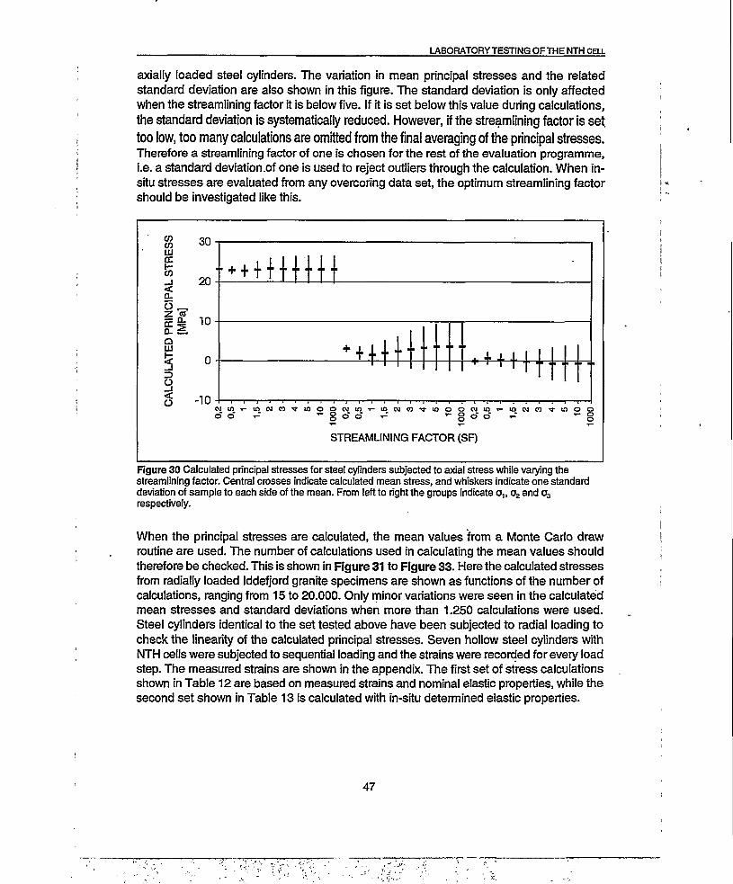
LABORATORY TESTING OFTHE NTH CELL
axially loaded steel cylinders. The variation in mean principal stresses and the related standard deviation are also shown in this figure. The standard deviation is only affected when the streamlining factor it is below five. If it is set below this value during calculations, the standard deviation is systematically reduced. However, if the streamlining factor is set too low, too many calculations are omitted from the final averaging of the principal stresses.Therefore a streamlining factor of one is chosen for the rest of the evaluation programme,i.e. a standard deviation .of one is used to reject outliers through the calculation. When in- situ stresses are evaluated from any overcoring data set, the optimum streamlining factor should be investigated like this.
Z m
tncMco^rmoocvto inwn'fiooown
STREAMLINING FACTOR (SF)
Figure 30 Calculated principal stresses for steel cylinders subjected to axial stress while varying the streamlining factor. Central crosses indicate calculated mean stress, and whiskers indicate one standard deviation of sample to each side of the mean. From left to right the groups indicate o,, o2 and o3 respectively.
When the principal stresses are calculated, the mean values from a Monte Carlo draw routine are used. The number of calculations used in calculating the mean values should therefore be checked. This is shown in Figure 31 to Figure 33. Here the calculated stresses from radially loaded Iddefjord granite specimens are shown as functions of the number of calculations, ranging from 15 to 20.000. Only minor variations were seen in the calculated mean stresses and standard deviations when more than 1.250 calculations were used. Steel cylinders identical to the set tested above have been subjected to radial loading to check the linearity of the calculated principal stresses. Seven hollow steel cylinders with NTH cells were subjected to sequential loading and the strains were recorded for every load step. The measured strains are shown in the appendix. The first set of stress calculations shown in Table 12 are based on measured strains and nominal elastic properties, while the second set shown in Table 13 is calculated with in-situ determined elastic properties.
47

LABORATORYTESTING OFTHE NTH CELL
B—B—S—B-n □ □ □ □0 1000 10000 Number of calculations
100000
Figure 31 Calculated mean major principal stress (diamond) and associated standard deviation (box) plotted as functions of number of Monte Carlo calculations for Iddefjord samples tested in the laboratory.
□ □■□□□□□□a10000010000
Number of calculations
Figure 32 Calculated mean intermediate principal stress (diamond) and associated standard deviation (box) as functions of number of Monte Carlo calculations for Iddefjord samples tested in the laboratory.
1.5 T
■a—b- c □ □2 0.5 -
-0.5 -
10000010 JO 1000 10000Number of calculations
Figure 33 Calculated mean minor principal stress (diamond) and associated standard deviation (box) as functions of number of Monte Carlo calculations for Iddefjord samples tested in the laboratory.
48

LABORATORY TESTING OF THE NTH CELL
The calculated major principal stress is normally smaller but very close to the applied stress, but at low applied radial stress it sometimes overestimated the applied radial stress. The intermediate principal stress always underestimates the applied radial stress. When in-situ elastic properties are used instead of nominal values, the calculated intermediate principal stress is even lower. If the a priori information, that the hollow core is loaded radially is used, the average calculated radial stress is underestimated by a few percent. The underestimation is larger when in-situ elastic properties instead of nominal elastic properties are used.
The calculated major and minor principal stresses with associated standard deviations are shown graphically in figures Figure 34 and Figure 35 when in-situ elastic properties are used. The calculated major principal stress is slightly underestimated and has a standard deviation that reduces to just above 3% of measured value for the largest applied stress. Even if a considerable standard deviation is associated to the calculated stresses, the absolute mean stress values are very close to the applied stresses. This observation suggests that the related standard deviations are unjust to the correctness of the absolute mean stress values, which implies that the calculated mean stress values are robust.
During radial loading of the hollow cores, a small axial tensile stress is predicted from the calculations. The associated standard deviation is more than twice the calculated tensile stress for all radial loads when nominal elastic properties are used. When in-situ elastic properties are used in the calculation of the stresses, the calculated tensile stress is lower for all radial load steps. This is probably caused because the outer ends of the hollow cores are not restricted and are therefore free to move axially. The relative standard deviation of the measured minor stress is very high, but if it is related to the active radial stress, it is in the same order as that of the major principal stress.
From studies of the orientations of the stresses, the calculated mean orientations are very robust. The orientation of any of the mean stress vector does not vary much with either the introduction of incorrect strain values, or the implicit variation in the measured strain or elastic properties. This can be seen in Table 12 and Table 13, and other tables where the orientation is given. Cancelling outlying or incorrect strain measurements before the calculation of the mean stresses however, leads to a reduction in their standard deviation, and is important to the final evaluation of the stress measurements. This is done by choosing an optimal streamlining factor that ensures both a stable set of mean stress values and reduces the standard deviations of the distributions. As part of the evaluation of the DISC computer code, Ruistuen [80] calculated the stresses from a set of overcoring measurements to show how the orientation of the mean principal stresses might change while outliers were subtracted from the data set. This was done by systematically reducing the allowable standard deviation (Streamlining Factor). A set of stereograms showing the orientations of all the calculated major principal stresses are shown in Figure 36 to Figure 39 where acceptable ranges of the major principal stress have been reduced from no limits through two to one. From the figures, the centre of gravity for the orientation of the principal stresses is almost unchanged despite the imposed limits.
49

LABORATORY TESTING OF THE NTH cell
• ••)••• S+1 ST.DEV
• •K*** S-1 ST.DEVSTRESS
40 - ST.DEVST.DEV%
RADIAL LOADING STRESS [MPa]
Figure 34 Calculated major principal stresses using streamline factor of one are shown for various loading steps. Upper and lower error band of one standard deviation (marked S+/-1 ST.DEV) are also shown together with absolute and relative standard deviation.
c«$CL
!
I
I
1
2
------1------S+1STJ3EV
--X---S-1ST.DEV
STRESS
RADIAL LOADING STRESS (MPa)
Figure 35 Calculated minor principal stresses using streamline factor of one are shown for various loadsteps. Upper and lower error band of one standard deviation (marked S+/-1 ST.DEV) are also shown together with absolute and relative standard deviation.
50

LABORATORYTESTING OFTHE NTH CELL
Table 12 Results from calculation of principal stresses (q) with DISC from radial loading (o6) of hollow steel cylinders containing NTH cells when nominal elastic parameters given by the manufacturer are used (E =21 OGPa and v = 0,30). <t> and 8 are orientations of the stresses.
Oe Stress o, s.d. <P 6[MPa] [MPa] [MPa] n n
4.8 o1 4.98 0.27 232 0o2 4.73 0.39 322 0o3 0.06 0.29 101 90
12.4 o1 12.34 0.48 226 002 11.92 0.81 316 0o3 -0.08 0.42 94 90
19.9 o1 20.00 0.66 218 002 19.11 1.34 308 003 -0.32 0.60 108 90
27.5 Ol 27.73 0.85 212 002 26.63 1.77 302 0o3 -0.38 0.76 108 90
35.0 o1 34.95 1.07 35 002 33.18 2.34 305 0o3 -0.73 1.03 127 90
42.5 o1 42.37 1.31 34 0o2 40.37 2.73 304 0o3 -0.78 1.20 128 90
Table 13 Results from calculation of principal stresses (oj with DISO from radial loading (oe) of hollow steel cylinders containing NTH cells when in-situ calculated elastic parameter are used, i.e. values for E and v calculated from biaxial tests of hollow cores with NTH cells). <f> and 8 are orientations of the stresses.
Oe Stress o, s.d. <P 8[MPa] [MPa] [MPa] [°] n
4.8 1 4.88 0.18 214 02 4.55 0.40 304 13 -0.10 0.23 104 89
12.4 1 12.19 0.41 216 02 11.47 0.84 306 03 -0.03 0.43 87 90
19.9 1 19.80 0.60 216 02 18.39 1.40 306 03 -0.19 0.71 106 90
27.5 1 27.62 0.79 215 02 25.80 1.99 305 03 -0.13 0.94 105 90
35.0 1 34.94 0.99 215 02 32.32 2.51 305 03 -0.27 1.20 120 90
42.5 1 42.34 1.27 216 02 39.30 2.90 306 03 -0.32 1.43 121 90
51

LABORATORY TESTING OFTHE NTH CELL
ODDA NCAL3D=20000
ORIENTATION OF MEAN PRINCIPAL STRESSES
Figure 36 Stereographic projection of mean principal stresses calculated using various streamlining factors (SF=1,2, none). Ruistuen [80]. No variation in orientation is experienced.
0DDA03 NCAL3D=20000 SF-1.0 a,
| PRINCIPAL STRESS ORIENTATION OF AIL POINTS 1
N
S
Figure 37 Stereographic projection of all calculated major principal stresses deviating less than one standard deviation from the total mean, showing a uniform distribution Ruistuen [80].
0DDA02 NCAL30=20000 SF=2.0 o,
| PRINCIPAL STRESS ORIENTATION OF ALL POINTS ~|
N
S
Figure 38 Stereographic projection of all calculated major principal stresses deviating less than two standard deviations from the total mean, showing a nonuniform or bimodal girdle distribution with some scatter Ruistuen [80].
ODDA01 NCAL3D=20000 NO STREAUUNING a,
| PRINCIPAL STRESS ORIENTATION OF ALL POINTS |
N
Figure 39 Stereographic projection of all calculated major principal stresses, showing a nonuniform or bimodal girdle distribution with excessive scatter Ruistuen [80].
52

LABORATORYTESTING OFTHE NTH CELL
Experiments including the number of overcoring measurements in the stress calculations are shown in Figure 40. First strains measured by only one NTH cell were used to calculate the principal stresses. Successively more data were included, to a total of eight independent overcoring strain sets. In the calculations a streamline factor of one was used. Surprisingly, the scatter is very low even when strains from only one overcored NTH cell is used. The third data set probably included incorrect strains caused by a bad cementing job, and thus significantly perturbing both the mean principal stresses and increasing the associated standard deviation. Introducing more overcoring strain data in the calculations seems to make the mean principal stress values more robust, while the associated standard deviations increase. In real measurements at least four to five successful sets of overcoring strains should be included in a proper conducted overcoring stress determination. This is done to keep the mean stresses as robust as possible with respect to unidentified outliers and to keep the standard deviation as low as possible.
+ + + + 'f
1 23456781 23456781 2345678
NUMBER OF MEASUREMENTS
Figure 40 Calculated principal stresses for steel cylinders subjected to axial stress while varying the number of datasets. Central crosses indicate calculated mean stress, and whiskers indicate one standard deviation of sample to each side of the mean. From left to right the groups indicate o„ o2 and o3 respectively.
53

LABORATORY TESTING OFTHE NTH CELL
Sensitivity of the NTH cell with respect to grain size
Three rock types have been collected; Larvikitt, Royken granite and Iddefjord granite, all with varying grain size. The rocks have been chosen to ensure variation with respect to grain size and mineralogic. Grain size and strength are shown in Table 14, while mineralogic composition determined by X-ray diffraction is shown in Table 15.
Table 14 Average grain size and tensile strength of rocks in test sample
Rock type Grain size (mm) Tensile strength (MPa)
Larvikitt 15 9.6Rayken Granite 5 10.2Iddefjord Granite 1 11.0
Table 15 Mineralogic composition of Iddefjordgranite, Raykengranite and Larvikitt determined by X-ray diffractogram analysis, courtesy of S. Bergstal (pers.com.)
IddefjordgraniteQuartz 27K-feidspar 28Plagioclase 39Combined feldspars PyroxeneBiotite 5AmphiboleClorite 1Magnetite traceApatite trace
Raykengranite Larvikitt37 28 33
8312
2 31
tracetrace 1
For all rock types the test samples have been prepared from one block and are cut along the same axis. The orientation of the measuring cells on the other hand, has been at random with respect to the borehole axis. After the overcored NTH cells were subjected to radial loading in the biaxial modulus chamber, the in-situ Youngs moduli and Poisson’s ratios were calculated. The measured strains are shown in the appendix. The calculated elastic properties and related standard deviations for each load step are shown in Table 16 and Figure 41 to Figure 46. Both mean values and single measurement values are shown. A significant scatter is seen throughout all tests, but the relative scatter decreases with increased loading, i.e. the standard deviation reduces to an almost constant value after initial loading. The scatter and observable variation bands are generally higher for the Poisson ratio than for Youngs modulus. Relative high standard deviations as seen in test results from Larvikitt and Royken granite obviously result from one or two NTH cells systematically operating as outliers. If the outliers are taken away, the variation band for Youngs modulus and Poisson’s ratio will be approximate 10 GPa and 0.06, respectively.
54

LABORATORYTESTING OFTHE NTH CELL
The absolute values of the, calculated elastic parameters increased during loading, but no ultimate levels were reached for any of the tests, although an assymptotic rate of increase was .seen. Two causes may explain this; either the rock and strain gauges are in poor contact, or micro fractures in the rock are closing during the initial loading of the cores. Furthermore, the variation bands for elastic parameters seem larger for the Fteyken granite test results than for the two others. This may be attributed to several factors, the ratio between length of the strain gauge and the grains, the mineral composition of the different rock samples, micro cracks in the rock mass and grain contacts. In the Iddefjord granite, the ratio between the strain gauge and the mineral grains are five to one, as proposed by the strain gauge manufacturers (Hottinger Baldwin Messtechnik) to give reasonable strain measurements. The Lanzikitt consists of almost only one mineral and the grain size is much larger than the strain gauge itself. The lack of other minerals seems to keep the variation in the elastic properties at a low level. In the Royken granite consisting of several minerals, the grain size is similar to the strain gauge length. This may lead to strain gauges in one NTH cell being bonded to minerals with vety different elastic properties, and thus to varying strain accommodation, which in turn scatters the results.
Table 16 Mean values for Youngs modulus and Poissons ratio and their standard deviations calculated from biaxial modulus chamber tests on overcored NTH cells in Iddefjord granite, Larvikittand Fteyken granite.
Rock type Stress Em** Esd Ynean v«Mpa GPa % %
Iddefjordgranite 1.2 24.20 13 0.137 153.2 28.82 12 0.140 115.2 30.79 11 0.145 117.2 32.49 11 0.153 10
10.0 36.50 10 0.167 1215.0 39.95 9 0.183 1120.0 42.61 9 0.197 10
Larvikitt 1.2 52.31 13 0.258 173.2 61.00 14 0.269 175.2 63.01 13 0.270 157.2 64.07 12 .0.277 14
10.0 67.80 11 0.279 2115.0 68.86 10 0.291 1820.0 69.27 10 0.299 18
Reyken granite 1.2 22.06 29 0.134 413.2 27.90 29 0.142 305.2 30.14 23 0.150 307.2 32.80 26 0.157 25
10.0 36.51 21 0.169 2315.0 40.67 22 0.185 2420.0 43.58 23 0.196 24
55

LABORATORY-TESTING OFTHE NTH CELL
I
I
Figure 41 Calculated Youngs moduli with mean values and standard deviation for each load step during biaxial loading of NTH cells in Iddefjordgranite
0.30 i+ ny
vmean
0.15-
0.10 -
0.05-
Radial stress [MPa]
Figure 42 Calculated Poisson ratios with mean values and standard deviation for each load step duringbiaxial loading of NTH cells in Iddefjordgranite
56

LABORATORY TESTING OF THE NTH CELL
50
40
-30 |
1T3
-20 S5
I- 10
00 5 10. 15 20 25
Radial stress [MPa]
Figure 43 Calculated Youngs moduli with mean values and standard deviation for each load step during biaxial loading of NTH cells in Latvikitt.
+ + +
—B—Emean
0.35 --40
0.25-
0.15-
+ ny
Q— vmean
-O—vsd0.05-
Radial stress[MPa]
Figure 44 Calculated Poisson ratio with mean values and standard deviation for each load step duringbiaxial loading of NTH cells in Larvikitt
57

LABORATORY TESTING OF THE NTH CELL
IT?II
Figure 45 Calculated Youngs moduli with mean values and standard deviation for each load step during biaxial loading of NTH cells in Roykengranite.
50
40
C030 1
1•g
20 roT3
I
10
00 5 10 15 20 25
Radial stress [MPa]
Figure 46 Calculated Poisson ratio with mean values and standard deviation for each load step duringbiaxial loading of NTH cells in Reykengranite.
+ ny■B—vmean
vsd
58

LABORATORYTESTING OFTHE NTH CELL
When the strains are measured and the elastic properties are calculated, the computer code DISO can be used to calculate the principal stresses and the related statistical variation. For each of the three rock types, the principal stresses are calculated in eight consecutive load steps. Calculated principal stresses‘differing more than on’e standard deviation from the mean values are not considered when the average stresses are calculated, i.e. a streamline factor of one is used. The complete results are shown in Table 17, while the calculated major principal stresses and relative standard deviation plotted versus the loading stress are shown in Figure 47 to Figure 49.
Biaxial overcoring experiments conducted under laboratory conditions show reasonable calculated principal stresses with consistent orientations. An almost one-to-one relationship, is found between the applied and the calculated major principal stress. The orientations of the calculated principal stresses show a minor variation at maximum 3 degrees off nominal. A maximum error of approximate 3 percent in prediction of the major, and 5 percent for the intermediate principal stress is seen in the tests. If the a priori information that the overcored NTH cells are subjected to a uniform biaxial stress is considered, a maximum error in the order of 2 percent is seen. However, this information is not appropriate to use in the present evaluation. Furthermore, the variation between the applied and the calculated axial stresses are of the same size as observed for the other two principal stresses, giving a high relative mismatch between the two.
Although the mean values are reasonablely accurate, the related standard deviations are relative high. The eight Rayken granite samples loaded to 20 MPa give a calculated mean value for the major principal stress of 20.2 MPa, an overestimation of 1 percent. Using the definition of the standard deviation of a normal distribution, there is a 95.5 percent probability that the mean value will be larger than 13.2 MPa and less than 27.2 MPa for the given sample. For all three rock types the standard deviation of the calculated stresses varies, but reduce as the loading increase.
The tests using Iddefjord granite has the lowest standard deviation of the calculated stresses while tests on Rayken granite samples has the largest. The standard deviation falls between the two for the tests using Larvikitt. There are principally two factors responsible for these relationships; grain size and petrography, but micro cracks and grain contacts may also play its part here. If the grain size is considerable smaller than the strain gauges, mineralogic composition has minor influence on the calculated principal stresses. If, on the other hand the grain size is in the order of the strain gauge, different strain gauges may be cemented to different minerals and produce significant variation. These effects are seen in samples of Iddefjord granite and Rayken granite respectively. In the Larvikitt that principally consists of micropertittic potassium feldspar and plagioclase crystals larger than the strain gauges, the standard deviation is not as much affected by the grain size as the Rayken granite.
59

LABORATORY TESTING OF THE NTH CELL
Table 17 Calculated principal stresses with standard deviations and orientation during biaxial loading for overcored NTH.cells in Iddefjordgranite (Idde), Larvikitt (Larv) and Roykengranite (Rayk).
Rock Po Oi sda, •sda, <t>(0,)8(o,)
% sda, sda. 8(0*) °3 sda. sda. 8(aJ
MPa MPa MPa % ° ° Mpa MPa % ° ° MPa MPa % ° °Idde 1.2 12 02 12 243 1 1.1 0.1 12 333 1 0.0 0.1 450 89 89
32 32 0.4 11 249 2 3.1 0.4 12 339 0 0.0 02 800 78 8852 52 0.6 10 250 2 5.0 0.5 10 340 0 0.0 02 485 74 8972 7.3 0.8 10 255 2 7.0 0.7 10 165 0 -0.1 02 522 70 89
10.0 10.0 0.8 7 234 1 9.6 0.9 8 144 0 -0.1 0.3 218 45 8915.0 15.0 1.1 7 234 1 14.4 12 8 144 0 -0.3 06 192 36 8920.0 19.9 1.4 6 234 1 19.2 1.4 7 143 1 -0.3 0.6 200 28 89
Larv 12 12 02 14 134 0 12 0.1 11 44 1 0.0 0.1 433 227 8932 3.3 0.4 13 120 1 32 02 11 30 1 0.0 02 428 241 8952 5.3 0.7 12 118 1 52 0.5 10 28 1 0.1 0.3 375 234 8972 7.3 0.9 11 139 0 72 0.7 9 49 1 0.1 0.4 421 234 89
10.0 10.1 1.0 10 13 1 9.7 0.9 8 103 0 0.1 06 700 206 8915.0 15.3 1.4 9 8 1 14.6 12 8 98 1 0.1 0.7 664 215 8920.0 21.2 2.4 11 346 0 20.3 1.8 8 76 2 0.1 1.8 1555 242 88
Rayk 12 1.3 0.4 27 307 2 12 0.3 22 37 2 0.0 0.1 800 178 8732 3.4 0.9 25 313 2 3.1 0.6 20 43 2 0.0 0.3 820 184 8752 5.4 1.3 24 328 2 5.0 1.0 19 58 1 0.1 0.4 484 171 8872 7.4 1.7 23 339 2 6.9 1.3 18 69 0 0.1 0.6 457 163 88
10.0 10.3 2.0 19 352 3 9.5 1.4 15 82 0 02 0.6 245 180 8715.0 152 2.8 18 354 2 14.2 2.0 14 264 0 0.3 0.9 252 174 8820.0 202 3.5 17 356 2 18.9 2.6 13 86 0 0.5 12 232 183 88
0 5 10 15 20 25
RADIAL STRESS [MPa]
Figure 47 Calculated major principal stress shown versus radial biaxial stress together with absolute and relative standard deviation in overcored Iddefjordgranite.
60

LABORATORY TESTING OF THE NTH CELL
S1 —©— S1sd S1sd%
RADIAL STRESS [MPa]
£
1§QQDC2
I111DC
Figure 48 Calculated major principal stress shown versus radial biaxial stress together with absolute and relative standard deviation in overcored Larvikitt.
i
i
■Q—S1 —e—S1sd —O—S1sd%--2520-
RADIAL STRESS [MPa]
<u!Q
IIi
Figure 49 Calculated major principal stress shown versus radial biaxial stress together with absolute and relative standard deviation in overcored Roykengranite.
i -!
i
i
i
61

LABORATORYTESTING OFTHE NTH CEIL
Discussion
Several factors affecting the NTH cell’s ability to reproduce strains under various loading conditions were investigated in the laboratory. SINTEFs code of practice was followed through , all operations during the tests that were run under favourable conditions. The results therefore show the best possible results that are obtainable with this overcoring technique. Effects of varying the following issues were investigated:
Axial loading of hollow cylinders incorporating NTH cellsRadial (biaxial) loading of hollow cylinders incorporating NTH cellsYoungs modulus of overcored hollow cylinders incorporating NTH cellsGrain size in overcored hollow cylinders incorporating NTH cellsExcluding outlying strain values from the stress calculationsNumber of overcored hollow cylinders incorporating NTH cells included in the stresscalculations
Before an analysis of the recorded strains from any overcoring device i.s conducted, the function of the device should be tested. The biaxial modulus chamber is the only feasible test method applicable for this in the field, and is also the most cost effective test method employed in the laboratory. During the tests of hollow metal cylinders with NTH cells the biaxial test always gave the most precise strain measurements, and was superior to uniaxial loading. This was caused partly by imprecise machining of the test samples and possibly by a non-coaxial load train in the uniaxial testing machine that both added to the overall discrepancy between the axial and radial test methods. If the mean strain values were used from the uniaxial tests this was corrected for, but still the scatter was high. Consequently, Youngs modulus and Poisson’s ratio were determined with the lowest scatter when the biaxial modulus chamber was employed.
The error in predicting the elastic properties for both test methods decreased as loading was increased. This effect reflected the errors inherent in the strain measuring process. Furthermore, the errors were relative lower for more ductile materials than for the stiffen The errors were inverse proportional to the absolute measured strains. Thus, for rocks with Youngs modulus in the order of 70 GPa, similar to aluminum, the errors in predicting Youngs modulus were almost negligible for stress levels within the tested stress interval. The Poisson ratio, however, was significantly underestimated, around 13 percent in low stress areas (<^<5 MPa), reducing to below 7 percent in high stress areas (a,>30 MPa).
When testing of the grain size effect were launched, the results obtained from metals testing were appreciated, and only biaxial loading was conducted to keep the possible scatter as low as possible. Measured strains and consequently calculated elastic properties were more scattered for the granular, rocks than for the metals. The calculated standard deviations for the elastic properties of Royken granite were almost twice as large as for the other two rocks. The main reason for this is the grain size being equal to the strain gauge size, i.e. the strain gauges may be cemented to various minerals having very different mechanical properties. Another reason may be micro cracks in the rock that seem responsible for the stress related variation of the calculated elastic properties. This was seen in all tests on
62

LABORATORY TESTING OF THE NTH CELL
rocks, but to a lesser degree in the tests on metals. When it was seen in the tests on metals, it had to be related to the cementing of the strain gauges. Tests conducted on the Iddefjord granite had the same relative standard deviation as those, on the Larvikitt. Although the calculated elastic parameters, grain size and mineralogy varied considerably, these tests gave the lowest standard deviations possible with this test method. The critical grain size or the largest scatter in standard deviations of the elastic properties occurred when the grain size of the host rock matched the strain gauge, i.e. five millimetres.
When the in-situ calculated elastic properties were used as input parameters to the calculation of the major principal stresses, an almost perfect match between the calculated and the applied biaxial stresses were obtained. Ideally both the major and the intermediate calculated principal stresses should have coincided, which they did not do. An average of 5 percent discrepancies between the two stresses may be found in biaxial testing. The discrepancy may likely become larger in uniaxial loading. An intrinsic assumption in the computer code assumed that all three stresses were unequal, and the statistical evaluation of the mean values systematically separated among the three and thus divided the principal stresses in three populations. As pointed out earlier, any a priori knowledge of this kind was unjustified in the evaluation of the calculated stresses, and was consequently omitted.
The calculated standard deviations of the mean principal stresses were identified to be the key factors in optimizing the calculation process. However, significant relative values were calculated, but they were always reduced as loading increased. Their relative value reduced as the number of overcored cells was reduced in the stress calculations. Despite the standard deviations of the principal stresses, both mean magnitude and orientation was always calculated with great precision.
Omitting outlying strains from the calculation of the principal stresses were a circumstantial process. It was done by first calculating the gross population and related statistical values. Then the calculations were done again and if the stresses from a single calculation deviated more than a specified part of the standard deviation from the mean the strain value was omitted from further calculations. When both orientation of the calculated stresses and the standard deviation of the magnitudes and the wish for a large population of solutions were considered, a pragmatical permissible range of one standard deviation of the mean stresses was set for future calculations. This is however a strict definition of outliers, in analytical chemistry, Garfield [81] defines an outlier to be definitive when it exceeds the mean value by more than three standard deviations. He also states that careful examination of values exceeding the mean value by more than two standard deviations are necessary.
The number of overcored NTH cells to be included in the in-situ determination of the full stress tensor should at least be four. This was based on practical experience because fewer measurements rendered the final stresses vulnerable to outliers which in turn would increase the standard deviation of the mean of the principal stresses and the precision of the mean itself.
The number of Monte Carlo draws included in the calculations of mean stresses and their standard deviations, should be close to, or the maximum allowable in the computer code,i.e. some 20.000. The number of calculations should be large to ensure as little effect of
63

LABORATORY TESTING OF THE NTH CELL
outlying or incorrect strains as possible, especially when measuring conditions are adverse. There are no positive effects in reducing the number of draws. A possible reduction in computing time is insignificant in the total measuring process.
Conclusions
Results of laboratory experiments where overcoring of NTH cells have been simulated andstrains measured have been shown. When the measured strains were related to the appliedstresses, the induced strains and nominal elastic constants, the following conclusions weremade:
a) The operation of all overcored NTH cells should be verified by use of the biaxial modulus chamber. This is preferential to axial loading of overcored cylinders.
b) Elastic properties to be used in the calculation of the principal stresses should exclusively be based on biaxial tests of overcored hollow rock cylinders with NTH
cells.c) When the stresses in-situ are non-coaxial, determination of the appropriate elastic
parameters to use in the calculation will be difficult. If the major principal stress is of main interest, elastic properties calculated from biaxial tests with strain levels comparable to the in-situ strains should give satisfactory stress results. If the minor principal stress is of interest, corresponding strains should be used in the calculation.
d) Most of the tests show measured strains always to be smaller or very close to the applied or induced strains. This is automatically corrected for if in-situ elastic properties based on biaxial chamber tests are used to calculate the principal stresses.
e) The relative errors of the measured strains are lower during radial loading than in axial loading.
f) The relative standard deviations of the measured strains decrease as the applied stress increases.
g) The relative standard deviations of the measured strains vary, where the lateral strains compared with the active load always have larger standard deviations.
h) Youngs modulus is underestimated, but the higher the loading, the better the NTH cell’s predictive ability.
i) Poisson’s ratio is underestimated.j) The relative error is larger for the estimates of Poisson’s ratio than for Youngs
modulus ..k) The standard deviations of the calculated stresses decrease systematically with
increasing Youngs modulus.l) Rocks with grain size comparable to the strain gauges, i.e. five millimetres, exhibit
the largest calculated standard deviations.m) Despite significant standard deviations of the calculated means of the principal
stresses, both their mean values and orientations are very robust to outliers.
64

LABORATORYTESTING OFTHE NTH CELL
n) It is recommended that at least four overcoring measurements are included in the calculation of the principal stresses and their orientation, and that an outlier rejection level of one standard deviation is used throughout the calculations.
o) The number of Monte Carlo draws in the calculations of the mean principal stresses and their standard deviations should be kept at a maximum of around 20.000 to reduce possible adverse effects of outlying strain values that are unidentified.
65

LABORATORYTESTING OFTHE NTH CELL
66

QUALITY RANKING OF STRESSES MEASURED BY THE NTH CELL
QUALITY RANKING OF STRESSES MEASURED BYTHE NTH CELL
When rock stresses are pursued either for an engineering solution or for general stress mapping, stress magnitudes are just as important as their orientations. The preceding chapters show how changes during the measuring process affect the NTH cell’s ability toassess rock stresses. In this chapter a quality ranking scheme for overcoring rock stress measurements by the NTH cell based on the stress magnitudes is proposed.
The data presented in the World Stress Map Project [82] focus on, and almost exclusively reports on orientations since the bulk of the data does not support quantification of absolute magnitudes. Focal mechanisms and breakouts account for 54 percent and 28 percent respectively, while hydraulic fracturing and overcoring measurements only account for 4.5 percent and 3.4 percent. Therefore, the World Stress Map quality ranking scheme seems unfit for assessing stresses measured by the NTH cell.
30.00 - -
20.00 - ■
10.00 — -
•10.00
20.00 30.00Calculated vertical stress [MPa]
40.00
Figure 50 Measured vertical stress plotted versus calculated vertical stress together with the theoretical relationship between the two. The abcissa values are based on measured densities and vertical overburden at measuring site.
67

QUALITY RANKING OF STRESSES MEASURED BY THE NTH CELL
Before this reevaluation of the calculated rock stresses, a pragmatic way of assessing the goodness of triaxial rock stress measurement results has been employed. It was based on the conception that normally the measured vertical stress (o„) equalled the calculated or theoretical vertical stress (aj. If this were observed, balance of forces in the rock was conserved and possible adverse effects related to the determination of the principal stresses all cancelled each other. Therefore it was argued that the calculated stress magnitudes and orientations represented good measurements. However, as shown in Figure 50, a considerable scatter in measurements is evident, and relative evaluation of several measuring results would not have been an easy task.
Evaluation of laboratory test results
In the preceding chapter, several factors were shown to influence on the calculated rock stress magnitudes. However, variations or scatter as shown by the relative standard deviation always reduces as the mean calculated principal stress increases. From these observations it follows that a lower limiting stress level represents a practical limit below which measurements should not be done. In Table 18 the relative standard deviation of the calculated major principal stresses are plotted versus the calculated major principal stresses for the laboratory tests of the NTH cells. Results for both rocks and metals are shown.
Figure 51 Relative standard deviation for the major principal stresses plotted versus calculated major principal stresses together with matching power law curves. All curve sets show reducing relative spread as stresses increase.
68

QUALITY RANKING OF STRESSES MEASURED BY THE NTH CELL
Table 18 Power equations for the curves fitted to the experimentally determined relative standard deviation of the major principal stresses (nO given as a function of the mean calculated major principal stress (o,)
Radially loaded steel cyl., nominal el.parameters (Steel-r, nominal):Radially loaded steel cyl., calculated el parameters (Steel-r, calculated): Axially loaded steel cyl., calculated el.parameters (Steel-a, calculated): Radially loaded al. cyl., calculated eLparameters (Alum-r, calculated):Radially loaded Iddefjord cyl., calculated eLparameters (Iddefjord, calculated): Radially loaded Iddefjord cyl., calculated el.parameters (Larvikitt, calculated): Radially loaded Iddefjord cyl., calculated el.parameters (Royken, calculated):
H,= 36.2236 o,'1-18305 H, = 4.4410 O, "°-12027 n,= 48.8355 a, ■°-38254
9.7593 oj"0-24542 q, = 18.3981 a, ■a3222S H1 = 16.3417o1 •°-16927 Hi = 33.77610, ‘°-21829
All the laboratory tests show a power decrease of the relative standard deviation as the major principal stresses increase. In Table 18 and Figure 51 the best fit curves are shown. The influences of radial versus axial loading of the overcored cylinders that were discussed earlier are also evident in Table 18. Here the axial loaded steel cylinders have a relative standard deviation that is almost an order of magnitude larger than radially loaded steel cylinders. Using nominal elastic parameters such as those given by the manufacturer of the two metals, also has an adverse effect on the calculated standard deviation of the mean principal stress. Compared with using calculated (in-situ) elastic parameters from the overcored cylinders, the nominal elastic parameters have largest influence for the lower stress levels.
To evaluate the effect of varying Youngs modulus, tests on aluminum and steel samples were conducted. The measured relative standard deviations for aluminum cylinders exceed steel cylinders, showing that under similar conditions, the material with the lower Youngs modulus has higher relative standard deviation. When all other properties are kept constant, these results suggest that higher measured strains imply higher relative standard deviations. Another likely factor responsible for these results is that the aluminum pipes were made by cold forming that infers an unknown elastic anisotropy in the material. This elastic anisotropy is not considered when the principal stresses are calculated.
In granular rocks, two effects affect the relative standard deviation of the calculated mean major principal stress simultaneously, grain size and Youngs modulus. The Iddefjord granite with grain size smaller than the strain gauges in the NTH cell, shows the lowest relative standard deviation. Higher standard deviations, but almost similar are the results from the Larvikitt samples. The Larvikitt is almost mono-crystalline and has grains that are larger than the strain gauges. The Royken granite whose average grain size equals the strain gauges, exhibits the largest relative standard deviation of all the calculated mean principal stresses. This is obvious when one strain gauge rosette may be measuring strains in a quartz grain while the others may measure strains in feldspars or micas. Youngs moduli also affects the variations in the results. Without a priori knowledge on neither grain size nor Youngs modulus, estimating how large the relative standard deviation of the mean major principal stress may be impossible. It must therefore be anticipated that the most adverse conditions apply. Under laboratory conditions, obtaining relative standard deviations of the major principal stress as low as 3 to 6 percent is possible at normal stress conditions. The lower value applies for relative high stress and vice versa.
69

QUALITY RANKING OF STRESSES MEASURED BYTHENTH CELL
Evaluation of field measuring results
All overcoring rock stress measuring results using the NTH cell were pooled in a database. Without any a priori information, establishing an experimental classification of the results based on the relative standard deviation of the mean major principal stress from the DISO calculations was then possible. These data can afterwards be used to assess the achievable field accuracy.
In Figure 52 the relative standard deviations of the three principal stresses are plotted as a function of the calculated mean principal stresses without any data reduction. In addition the power type best fit curve for each principal stress is given. The best fit power curves for the calculated mean stresses without streamlining are given by the equations:
Hn =218.526 d*0'463282 n2 = 166.155 a2"°A98677
' n3 = 641.700 a3 *°'812411where:
Hj denote the relative standard deviation of the i’th mean principal stress
As in the previous figure, the similar data are plotted in Figure 53. In this figure they arecorrected such that outliers exceeding one standard deviation are rejected in the finalcalculation using DISO, reducing the overall spread in the population. Best fit power curves for the calculations with streamlining of one standard deviation give the following relationships:
Hi = 140.783 n2 = 97.5432 H3 = 242.163
a -0.59806401 -0.601068_2 -0.729348 °3
From both sets of calculations, the distributions of the relative standard deviation of the intermediate principal stress (a2) gave the lowest relative standard deviation of the mean. The reason for this is that all calculated intermediate principal stresses are bound by the major and minor principal stresses. Thus, a narrow distribution of the intermediate principal stress is created. The distributions of the major and minor principal stresses have relative long tails extending upwards and downwards respectively.
To set up a quality ranking scheme, the quality ranking should be coupled to the standard deviation for each of the principal stresses. However, since all three standard deviations are monotonous decreasing with increasing stress, considering one of them is sufficient. The quality ranking can therefore be related to any principal stress, and it is here chosen to relate it to the calculated mean major principal stress.
70

QUALITY RANKING OF STRESSES MEASURED BY THE NTH CELL
10000 -q-
1000 —
+ Usjorprinelpalstress# Intermediate principal stress
X Minor principalstress
T—rTTTTT i i urn1.0 10.0
Calculated mean principalstress [MPa]100.0
Figure 52 Relative standard deviation of mean stresses plotted versus calculated mean stress for all three principal stresses together with best of fit lines. No data reduction has been used.
10000
Ma|orprinclp!e stress *
Intermediate principal stress
Mhorprfnclpal stress
100.0Calculated mean principal stress [MPa]
Figure 53 Relative standard deviation of mean stresses plotted versus calculated mean stress for all three principal stresses together with best of fit lines. During calculation values exceeding one standard deviation are rejected.
!
71

QUALITY RANKING OF STRESSES MEASURED BYTHE NTH CELL
10000.00 T—TT1—l l l l 11 l I I I 11
1000.00
100.00
/Average + 2,0 st.dev. A Average + 1,5 st.dev. C- Average + 1,0 st.dev. Average + 0,5 st.dev. Average
Average - 0,5 st.dev.
10.00
Average -1,0 st.dev. ■
Average -1,5 st.dev
Average - 2,0 st.dev.
I I I I I I II I JTTTTI I I I III
100.00Calculated mean major principle stress [MPa]
Figure 54 Relative standard deviation of the mean major principal stresses plotted versus calculated mean major principal stresses together with the best of fit power curve. Lines showing confidence limits are added.
In Figure 54 the relative standard deviation of the mean major principal stress is plotted versus the mean major principal stress. The best fit power law curve is drawn in blue through the data. From statistical theory if a sample is Gaussian distributed, the mean and standard deviation fully describes the distribution. Under this assumption some confidence limits to the fitted power equation are calculated and drawn in red. The line marked “Average” is the best fit power curve to the data and shows the locus of 50 percent of the observations. Furthermore the line marked “Average -1,0 st.dev." shows that approximate 16 percent of the data fall below this line and so forth. The sample is skewed to the low end side of the relative standard deviation of the calculated stresses and therefore not exactly Gaussian distributed. Since it is the lower part of the distribution that is of interest, assuming Gaussian distribution is unimportant for the sought quality ranking. The low-end tail of the distribution below a major principal stress of 3 MPa consist of few measurements. These measurements consequently have intermediate and minor principal stresses approaching the lower limit for the strain gauges. The laboratory measurements shown earlier in this chapter were superimposed on the field confidence grid in Figure 55. Thus, measuring results with the best achievable quality can be related to the field results. Two features can be seen here; the relative standard deviation of the laboratory samples has lower variability with stress magnitude and is lower compared with the field results.
72

QUALITY RANKING OF STRESSES MEASURED BY THE NTH CELL
IIi S
=J OCO o
.2><DT3
"5COT3C
2CO
"occ
10000.00 -=r
1000.00
100.00
10.00 —
1.00
0.10
Average + 2,0 sl.dev. Average +1.5 st.dev. Average +1.0 st.dev.
Average + 0,5 st.dev. Average
Average - 0,5 st.dev.
Average • 1,0 sl.dev.
Average-1,5 sl.dev
T Average - 2,0 st.dev.
I I I I I 11
1.00 10.00 Calculated mean major principle stress [MPa]
Figure 55 Laboratory stress data plotted in the field derived confidence graph obtained in the previous figure.
Several observations can be deduced from Figure 54 and Figure 55:
• The associated relative standard deviation of the calculated stresses from field measurements decrease with increasing measured major principal stress.
• The associated relative standard deviation of the calculated stresses from field measurements are centred when compared with the confidence grid.
• Possible outlying or incorrect field measurements can be detected by overlaying the confidence grid on these plots.
• In field measurements caution should be observed if mean major principal stresses lower than 3 MPa is returned from the calculations.
• Under controlled conditions in the laboratory, relative standard deviation of the calculated stress is lower than in the field.
• Under controlled conditions in the laboratory, the variability of calculated stresses over various stress ranges is lower than in the field.
73

QUALITY RANKING OF STRESSES MEASURED BYTHE NTH CELL
Discussions
In the-preceding paragraphs and chapters various factors influencing on the variation of the calculated stresses have been discussed. Some contribute more than others to the uncertainty in the final assessment of the given stresses. From beginning to end emphasis has been put on the stress magnitude and its variability given as its relative standard deviation. The disregard of a classification scheme related to the orientation of the stresses is justified by the stereograms presented by Ruistuen [80]. Based on DISC calculations, he showed that the calculated orientations were almost unaltered by considerable variations in the measured strain values. Realising this, a quality ranking similarly to Zoback’s (op.cit.) scheme for the World Stress Map focussed on orientation alone, would not justify the merit inherent in the overcoring measurements.
To devise an empirical quality ranking for overcoring rock stress measurements, results from both field and laboratory measurements have to be merged. The field measurements give the overall real variations that must be expected including effects of outliers and very good measurements, while the laboratory measurements reveal the lowest variation obtainable. In this way, all sources of variation through the complete measuring chain are possible to embrace in two parameters, the calculated mean major principal stress and its relative standard deviation.
The quality ranking is set up and divided in several groups where the best group is called Group A and progressively the quality deteriorates through Group D that is the lowest grade. Group B and Group C contains intermediate quality measurements. Group A must contain the top quality laboratory measurements and the top quality part of the field measurements. Group B and Group C are two intermediate groups while Group D contains the outliers and possibly incorrect data. The Gaussian confidence grid of the field data with the laboratory data on top shown in Figure 55 was used for this purpose. Additional fences limiting the quality groups are set in the stress domain.
The lines called “Average -1,0 st.dev”, “Average” and “Average + 1,0 st.dev.” provide easy conceivable border lines and divides the four quality groups. A similar set of dividing lines can be defined along the calculated mean major principal stress axis. If the major principal stress is below 1 MPa, the two other principal stresses cannot be determined with any satisfactory relative standard deviation, therefore 1 MPa is set as the upper stress bond for the worst classification. The relative standard deviation of field data decreases significantly when the major principal stress exceeds 3 MPa. Furthermore, when the major principal stress exceeds 3MPa, the other two principal stresses can normally be calculated with sufficient low relative standard deviation and so this is chosen as the lower stress bond for the highest quality measurements. The intermediate groups are then divided in the remaining middle at 2 MPa.
74

QUALITY RANKING OF STRESSES MEASURED BY THE NTH CELL
Conclusions
Triaxial overcoring rock stress measurements with the NTH cell evaluated by the computer code DISC shown in an earlier chapter can be quality ranked according to the calculated magnitude of the major principal stress and its relative standard deviation. This is shown in Figure 56 and Table 19. Four empirically determined quality groups are devised, ranging from the highest quality called Group A through the lowest Group D. The bulk part of field measurements until now classifies as Group B and Group C, while laboratory tests under controlled conditions classify as Group A and B depending on rock types and test conditions.
10000.00 —=r
0.10 1.00 2.00 3.00 10.00 100.00_________ ________ __ Calculated mean major principle stress fMPal______________
Figure 56 Quality ranking of overcoring rock stress measurements are based on the calculated major mean principal stress and its relative standard deviation. The calculated stresses are thus assigned one of four groupes of which Group A comprises the highest quality measurements and Group D the lowest quality. In the figure the following lines are marked where Qi is relative standard deviation of calculated stress, and o, is calculated mean major principal stress:
Line AB: q, = 44.7-a/5331 Line BC: Hi = 140.8 o/^ Line CD: q, =236.9-o1‘a593'
5f
75

QUALITY RANKING OF STRESSES MEASURED BYTHE NTH CELL
Table 19 Quality ranking limits dividing overcoring rock stress measurement in four groupes according to the calculated mean major principal stress and its relative standard deviation
Group A: o, >3 MPa and m a 44.7-a1"a59s’
Group B: o, >2 MPa and p1 s MO.S-o^ 598' and
o, £ 3 MPa and Hi > 44.7-a^-5981
Group C: a, > 1 MPa and Qi s 236.9o^^'
s 2 MPa and m > 140.8-o1"a5981 and
GroupD: < 1 MPa and n1 > 236.9-a1‘a598'
i
|i
!
I
76

RECALCULATED ROCK STRESSES AND IMPLICATIONS TO THE REGIONAL STRESS FIELD
RECALCULATED ROCK STRESSES AND IMPLICATIONS TO THE REGIONAL STRESS FIELD
All available information on three-dimensional rock stress measurements using the NTH cell. have been traced in both NTH and SINTEF archives, dating from its initial development to 1992. Some reports written later have also been investigated. To expel any ambiguities in the calculated rock stresses, all information pertinent to a proper evaluation such as vertical overburden, elastic properties, measured strains and measuring borehole orientation were controlled. Any reports missing some of this information were omitted from the recalculation scheme. Thus, measurements from some 150 sites could be further processed according to the recommended code of practice for evaluation of overcoring rock stress measurements developed in the preceding chapters. The recalculated three-dimensional rock stresses shown in Table 20 and Table 21 make up results from all the available reports with complete input data sets on three-dimensional rock stress measurements using the NTH cell that has been available for this work. During collation of the present database, a preliminary version was published by Fejerskov et.al. [83] where the authors in detail elaborate on the orientation aspect of the stresses. The calculated stresses on which their work is based has not been subjected to outlier rejection by application of the streamlining factor. Since they only deal with the stress orientations, this is of minor influence due to the robustness of the calculation scheme.
Representation of recalculated rock stresses
From the 155 measurements presented in the in Table 20 and Table 21, five measurements get the quality rank A, 73 get B, 53 get C and 24 get D respectively. The quality rank D measurements are rejected in the further analysis due to an excessive scatter. Near - surface effects considerably affect the horizontal - and vertical stress components and lead to relative high compressive or occasionally tensile horizontal stresses at shallow depths. Furthermore, the vertical overburden is probably imprecisely given, causing an excessive scatter if it is used in analysis of the measurements.
77

RECALCULATED ROCK STRESSES AND IMPLICATIONS TO THE REGIONAL STRESS FIELD
Table 20 First part of the calculated principal stresses and their orientations together with horizontal- and vertical components. To each measurement location and coordinates are given including quality ranking and the standard deviation of the stress magnitudes. For reference theoretical vertical and horizontal stresses are calculated. For a description of the column heading refer to Table 22.
rS3SOIS3TR
AUNEXAIttGN AUNEKAMMENOIBLEKVASSU BLEKVASSU01B&KVASSU BIEKVASSU01 ‘BLEKVASSU 5LEKVASSCD1BLEKVASSU BLEKVASSUO ial 215SgURUWHISMM 2*4BOXEN. SVEWG 222BOUDEN. SVBUG IK 11SOCCER SVERG 23.71 275
6ll 325BYKLEC1 Hotel 111 3StfQECSHotan 111 122BYKLE03H*a 1.11 23
2.71 85OAZENOtTddca 221 15S
OAWEUORA.SVER DANNEU0RA01 HI 135IM 167111 335
Ocwtimwildcel* Drammamrialamam Oil 1662M S*111 112Ai 306
FJAERLAND 72l 283FJOetWIAFJORO 275
FOSOAIEN 12S0 325Mi 2421S| S3
GRENGES8EFG.SV GRENGESBEAG01 110005 1*1 112GRENGES8ERC.SV 6RENGES8ERG02 *-21 122GRENRF2SRERG.SV GRENGES8ERG03 Atl 11*GRENQES8ERO.SV GREN6ESBER604 121 203
oi| ISOGRONQtiOUA GRONGtiOUAGUTTUSJO.SYER1 GUTTUSJ001
l$j 82
KtARTOEY 121 3501*.l| 352
278HOCANDSFJORO H0W6AO901 *eI ts
HOUlESTRAf© HOCWESTRAND01 59.4200 C 02 0.11 30
HOYANGEfi HeywowOt F77012 612147 6.1036 0 650 215 47A 230 8 132 321 10 S1E| 01 79 17 tit 135 28.0 IS
HOYANGER Hcymo*f1 F7B0U 612147 6.1036 C 600 28.1 6.9 218 15 20A 32 341 64 152 Si| 122 21 204 16X1 12$ 27.6 35 23A 6.1
Hueefli F7932S 72597 8 Ui 92 14 177 32 42 1.7 302 44 2.6 zsl to 25 S3 34 61 U 171 34 MJOSSJNGFJORO 3l| 43 12
7b| 155JOSTEOAL/VGOAL iaMaoWioaK AT) 313
33| 18lit 602.7) 61K1 23
KLEPPEN.NAUSOS 2ll 3*6Ke±be*6*nfltgmHWr Kcew SwflMn HWT 11 23KobbeNKcbbefrPS Kcbbafc KctbaM PSKcbbekKebbitifHWT KofcbahrKcfcbatirKWT IK 301itobbekLewn Kabbthltranm 1*J 256KcfcbeUUWrd KatbatobBaand Sll 358Kabtxli [lirrijiTTi KcbbatoRaavtaaan
LAJSVALL.SVER1 UUSVALL01UWEFJORO 17j 323UASEROSLO 0H 329UUNGAVERK.SVE UUNOAVERKOI 2H 182UUN6AVERX.SVE UUNGAVERX02UUNGAVEfUCSVE UUNGAVERX03LOEKKENVEttt LeldtarOKAaate)lOEXKENVERK Lati=erC2(Asete> zsi UTLOEKXENVERK LOEXKENVERX02LOEKKENVERX Til 55
LYSEFJCROGN/TXOAN Lvaefiertartii/nedm A6l 167UAURANGER UAURANGER 31UAURANGER 8A| 127wtimadBn»aa Uaueadoi Bmat 111 16
12t 37UOIRANA UOIRANA61 60a| 263UOiRANAUOIRANA
J
78

RECALCULATED ROCK STRESSES AND IMPLICATIONS TO THE REGIONAL STRESS FIELD
Table 21 Second part of the calculated principal stresses and their orientations together with horizontal- and vertical components. To each measurement location and coordinates are given including quality ranking and the standard deviation of the stress magnitudes. For reference theoretical vertical and horizontal stresses are calculated. For a description of the column heading refer to Table 22.
SH2M|tswaoiSHty|SHToK
N£SUOEN,SVtitiHEStPEN. SVEWNESUOEH. SV6R1
<0X660 <562810 St-<1.18001 »<400|C 53) 1081 1431 3.1| 08
~5fn
RartruJdAOfiTXIaRuttrjidl Voi*efc8» 164! 80) 4J 6.71 1251 Z6| 1.1RAUTUVAARA. ft* RALTTUVAARA01RAUTUVAARA.FH RAUTUVAARAOZ
921 2X2l 21 10.1) 13RAUTUVAARA. FW RAUTUVAARA33RAt/TUYAARA. FW RAUTUVAARAOIRIOT WTO SPAMRIOT WTO. SPAN
2361 KflOg 10X1 1581 11.71 2-4331 1031 1231 11JI <3
=#=ea-aeea 173136<63883 17X800 «a
<31 1191 ll.lt 64
ISTORPORSHEI<1X938 73147
— - ~7S|~SJM*n802Gfc4ftl
miSdMttwCOGfcAnB 2861 201 113
s<j<4>moi crariemSU<1it802Ch»rtaB>SJ44h8COOmrio88&3848M01 GtorvO*SiA4«*n*01 Saqno
SYDVARAHOER SYOVARANQ£ft0133SYOVARANOER iSYPVARRHGER02-71
1431SYDVARAWGER SYDVARASOER0334SYDVARAWOER SYDVA8ANGER0430SYDVARANGSR SYDVARAHGEfiOSXO 1
ilr ~73TivKAfjea^AuoeeflQ RAU06ERG GRUYES*4~ 371 1Z8I 127}
l
i
l79

RECALCULATED ROCK STRESSES AND IMPLICATIONS TO THE REGIONAL STRESS FIELD
Table 22 Explanation of abbreviations used in the overcoring rock stress summary
Project Name Project name used by SINTEF to distinguish the measuring sites Borehole Name Name of the borehole where the overcoring measurements have been done Report Part of SINTEF’s report identifier where the first letter is an identifier, the next two digits
represent the year of the measurement and the last three digits is an identifier number.If the number is given as a four-digit number, it represents the year of the measurement and no formal report excists
Lat.(dec) Decimal latitude of measuring site Lon.(dec) Decimal longitude of measuring site Grade Quality ranking of the total measurementOB Vertical overburden [m]SiM Computed i'th mean principal stressSiSD Computed standard deviation of i’th mean principal stressSiTR Computed trend of i’th mean principal stressSiP Computed plunge of i’th mean principal stressISVM Vertical component of the measured three-dimensional stress field1SH2M Minor horizontal component of the measured three-dimensional stress fieldISH20 Orientation of the minor horizontal component of the measured three-dimensional stress
fieldISH1M Major horizontal component of the measured three-dimensional stress fieldISH10 Orientation of the major horizontal component of the measured three-dimensional stress
fieldGV Theoretical vertical stressGH Theoretical horizontal stress
To present the results from all overcoring rock stress measurements in a planar map, a new presentation method is devised. In every measuring location the measured vertical major- and minor horizontal stresses are drawn. The two horizontal stresses are plotted as vectors with true orientation while the vertical stress is plotted as a circle on top of them. With the same origin, the theoretical vertical and horizontal stress are plotted as blue circles for comparison. All stresses in each location are normalized by the theoretical vertical stress, which is given as unity. The various stresses are colour coded to differentiate between them. Red is assigned to the major principal stress vector wile black is assigned to the minor horizontal stress vector and their quality grouping. An explanation of the quality rating of the stresses are given in Table 24. In all maps, quality group D stress results are omitted and represented by the theoretical vertical stress symbol only. The map view presentation shown in Figure "57 can be used to illustrate the measured stresses as far as measuring results are available throughout Norway, Sweden and Finland. Telling the quality of the measured rock stresses is also possible. However, the rock stresses vary considerably since they are measured in different formations and at different depths.
80

RECALCULATED ROCK STRESSES AND IMPLICATIONS TO THE REGIONAL STRESS FIELD
Figure 57 Map showing location, quality grade, orientation and magnitude of horizontal and vertical stress components for all reevaluatedstresses measured by the NTH cell in Norway, Sweden and Finland. All measurements are conducted by NTH / SINTEF. In this figure, all radii and vectors represent nominal stress values of horizontal and vertical, theoretical and vertical stresses respectively.The colour coding of the symbols identify theoretical and measured vertical stresses, major and minor horizontal stresses and the quality ranking of the measurements. Group D measurements that are the lowest quality designation are represented by unity circle only, to locate the measurement point.
81

RECALCULATED ROCK STRESSES AND IMPLICATIONS TO THE REGIONAL STRESS FIELD
Comparing measuring results presented in Figure 57 without any interpretation is difficult. To evade this problem, the stresses are normalized by the measured vertical stress component and grouped in order of thrust- (reverse), strike-slip- and normal faulting regimes. The faulting regimes are furthermore defined from the horizontal and vertical stress components of the measured stresses as shown in Table 23. In all measuring locations the measured vertical -, major - and minor horizontal stresses are normalized by the measured vertical stress. The two normalized horizontal stresses are plotted as vectors with true orientation while the normalized vertical stress is plotted as a circle on top of them. With the same origin, the normalized theoretical vertical and horizontal stresses are plotted as circles for comparison. The colour coding and map symbol is similar to what is shown for the nominal measured stresses. An example of the completed symbol is shown in Figure 58, while the coding is presented in Table 24.
Table 23 Definition of faulting regimes based on measured vertical and horizontal stresses
Normal faulting regime ov a oH a ohThrust faulting regime oHaova ohStrike slip faulting regime crH a oh £ ov
where:ov Measured vertical stressoH Measured major horizontal stressoh Measured minor horizontal stress
By evaluating the maps in Figure 59, Figure 60 and Figure 61, it can be distinguished whether the rock mass at the measuring site is in a relaxed gravitational stress state, or if higher stresses are present, which tectonic regime is predominant.
To appreciate the stress regimes outlined above, the measured and theoretical vertical stresses shown in Figure 62 must be evaluated. From the figure, considerable variation is evident no matter the quality rating of the measurements. Also some probable imprecise overburden values are given at, e.g. the depth intervals 300,400 and 450 metres. Without considering the nature of this variability, the measured stress components evidently have to be related to the measured -, and not the theoretical vertical stresses. This is shown in Figure 63, where the three measured stress components, the vertical, and two horizontal stresses are normalized by the measured vertical stress and displayed as a function of the measured vertical stress. The normalized vertical stresses are given as unity. As the vertical stress increase and correspondingly the overburden increases, the horizontal stresses reduce to become lower than the overburden. Although only few measurements are obtained below some 700 metres, they clearly show the magnitude of the horizontal stresses to be inferior to the vertical stress.
82

RECALCULATED ROCK STRESSES AND IMPLICATIONS TO THE REGIONAL STRESS FIELD
Orientation angle with reference to geographic northNorm, major horizontal stress
Norm, vertical stress
Norm, theor. vertical stress
Norm, theor. horizontal stress
Norm, minor horizontal stress
Figure 58 Symbol used in maps describing measured rock stresses. The symbol relates measured horizontal and vertical stress components to their theoretical counterparts in addition to show the orientation of the horizontal stress components.
Table 24 Explanation of the four different symbols used to distinguish between the quality rankings or grades in maps presenting overcoring rock stress measurements
Quality rank Color Symbol
Grade A Black Full symbol with (normalized) ISVM colour coded blackGrade B Red Full symbol with (normalized) ISVM colour coded redGrade C Yellow Full symbol with (normalized) ISVM colour coded yellowGrade D Blue Only (normalized) theoretical stresses in blue marked D
83

RECALCULATED ROCK STRESSES AND IMPLICATIONS TO THE REGIONAL STRESS FIELD
Figure 59 Map showing horizontal and vertical stress components normalized by the measured vertical stress for measurements indicating thrust faulting regimes. Quality grade and orientation are also given. For reference normalized theoretical vertical and horizontal stresses are indicated. The colour coding of the symbols identify theoretical and measured stresses, major and minor horizontal stresses and the quality ranking of the measurements. Group D measurements that are the lowest quality designation are represented by unity circle only.
84

RECALCULATED ROCK STRESSES AND IMPLICATIONS TO THE REGIONAL STRESS FIELD
i
Figure 60 Map showing horizontal and vertical stress components normalized by the measured vertical stress for measurements indicating strike-slip faulting regimes. Quality grade and orientation are also given. For reference normalized theoretical vertical- and horizontal stresses are indicated. The colour coding of the symbols identify theoretical and measured stresses, major and minor horizontal stresses and the quality ranking of the measurements. Group D measurements that are the lowest quality designation are represented by unity circle only.
85

RECALCULATED ROCK STRESSES AND IMPLICATIONS TO THE REGIONAL STRESS FIELD
Figure 61 Map showing horizontal and vertical stress components normalized by the measured vertical stress for measurements indicating normal faulting regimes. Quality grade and orientation are also given. For reference normalized theoretical vertical and horizontal stresses are indicated. The colour coding of the symbols identify theoretical and measured stresses, major and minor horizontal stresses and the quality ranking of the measurements. Group D measurements that are the lowest quality designation are represented by unity circle only.
86

RECALCULATED ROCK STRESSES AND IMPLICATIONS TO THE REGIONAL STRESS FIELD
Vertical overburden (mlFigure 62 Vertical measured and theoretical stresses plotted versus vertical overburden at measuring site. For the measured stresses the plotting symbols are exchanged with their respective quality rating letter. The best fit line is drawn through the theoretical vertical stress values that are calculated based on laboratory density measurements. Significant scatter around the theoretical values are evident regardless of the quality rating of the measured stresses.
10 — + Noanolzed mojoi hottontcl is«u
O Notmotiid minor horttonioltireu
Measured vertical stress (MPa)Figure 63 Normalized major and minor horizontal stress components except quality group D as a function of vertical overburden. All data presented in this figure are plotted in the map in Figure 57. Significant scatter in the measured data are found when the vertical stress are below some 7 MPa corresponding to less than 250 m vertical overburden.
87

RECALCULATED ROCK STRESSES AND IMPLICATIONS TO THE REGIONAL STRESS FIELD
Discussion of rock stress measurements
From the preceding tables and graphs, no simple geographical relationships between any measured stresses or orientations can be found. In Figure 64, however, notched Box and Whisker plots of the measured stresses grouped according to stress regimes are drawn versus the measured vertical stresses. The figure shows that the indicated faulting regimes are dependent on the vertical stress, or indirectly of the vertical overburden. Thrust faulting regimes are favoured at shallow depth followed by strike slip faulting regimes before normal faulting regimes are picked up in the deeper measurements. This suggests that in a crustal perspective, the measured high horizontal stresses are a surface related phenomenon.
Measured vertical stress IMPa]
Figure 64 Notched box plots of the measured vertical stresses grouped according to faulting regime. T denotes thrust faulting regime, S denotes strike slip faulting regime and N denotes normal faulting regime. Measured vertical stress is indicative of the overburden at the measuring site. The graph thus shows that thrust faulting is likely to occure close to surface and normal faulting will prominent at larger depths with strike slip faulting in between.
If the measuring results are subjected to principal component analysis (PCA), the inherent co-variation or variance in the sample can be evaluated. PGA is based on a linear description of the input data. For the measured rock stresses, orientation and overburden, this has been done according to standard procedures as described by the statistical program package SYSTAT [84]. If many factors are used to describe the variation within the sample, considerable random error is described. In the evaluation of the stresses and their orientation, only six factors explain some 80 percent of the inherent variance in the sample. These six factors’ relative importance, or explanation of the inherent variance in the sample, are shown in Table 25. This is also the factors used during the following analysis.
88

RECALCULATED ROCK STRESSES AND IMPLICATIONS TO THE REGIONAL STRESS FIELD
Table 25 Percentage of variance explained by each rotated factor in the principal component analysis
Factor number 1 2 3 4 5 6Percent variance explained 26.5 19.0 14.0 10.7 10.0 8.6
In Table 26, loadings for the six factors for all input variables are shown. The absolute loadings vary from naught to one, where one suggests high influence to the factor. A simple structure is discemable in Table 26. The first factor describes the most significant variation in the sample, and lesser distinct patterns follow in subsequent factors. Furthermore, if several variables have absolute high loadings within one factor, covariation between the variables is observed. If they have opposite signs, the relations between the variables are inverse.
Without any a priori assumptions, the PCA groups and ranks the variables as shown in Table 26. The most dominant variables make up factor 1, consisting of the relative standard deviation of the stress magnitudes. Factor 2 principally deals with the stress magnitudes and to a lesser degree the vertical overburden. The rest of the factors are less important to the variation in the sample, but systematically deal with strike and plunge of the various stresses. Another feature observed in the loadings, is that almost no cross influence between the various factors are visible, i.e. high loadings are only found in one factor, and thus the variables are almost independent of each other.
Table 26 Loadings for the rotated six most prominent factors of the recalculated stresses. Explanation of the variables constituting the factors are given in Table 22
Factor! Factor2 Factors Factor4 Factors FactorsS3SD .989 -.004 .006 .051 -.020 .008S1SD .975 .044 -.002 .007 -.038 .026S2SD .961 .189 .025 .060 .015 .026S2M .075 .942 .047 .021 -.001 .046S1M .245 .872 .047 .052 .004 .075S3M -.112 .831 -.038 -.102 .072 -.039OB .094 .671 -.108 .071 -.426 -.017S2P -.018 -.011 -.976 .007 .197 -.011S3P .008 -.040 .803 .046 .573 .004S3TR .055 -.056 .006 .888 .066 .264S1TR -.063 -.093 -.021 -.737 .007 .538S1P .016 .026 .043 -.060 -.974 -.027S2TR -.055 -.072 -.016 -.082 -.026 -.936
89

RECALCULATED ROCK STRESSES AND IMPLICATIONS TO THE REGIONAL STRESS FIELD
The relative standard deviation of the stress magnitudes co-variate and all go into factor one. This is a clear confirmation that the quality rank designation proposed in the previous chapter is a viable method. In Figure 65 the factor scores for all observation sets (rock stress measurements) are drawn in the factor 1 - factor 2 plane with the respective box and whiskers plots for each factor score. From the box and whiskers plot of the factor score of factor 1, seven observations are classified as far outliers and three observations as near outliers. Furthermore the hinges show a distribution skewed towards the low side. This shows outliers at the high end, or suggests that stresses having high relative standard deviations are outliers.
Towards the low end of the factor score of factor 2 an increase in factor score for factor 1 is evident. This may also point to outliers or incorrect measuring points at relative low overburden. If the outliers in the factor score of factor 1 are rejected, a systematic positive relation between the two factor scores is evident in the plot. The outliers are evenly distributed and related to the sample frequency more than the stress level as suggested by the factor score of factor 2. Both observations point to, and support the conclusions in the previous chapter where quality ranking designation D (lowest) was assigned to measurements with high relative standard deviations of the mean stresses. The outliers in the factor score of factor 2 only suggest that few rock stress measurements have been conducted in areas of high stresses or in areas with large overburden. This is only related to the sample distribution itself and cannot be termed outliers in a measuring perspective.
®s uo
4 .:FACTOR SCORE (2)Figure 65 Plot of factor scores one versus factor scores two in the principal component analysis. Factor score one represents the relative standard deviation of the stresses, while factor score two represents the stress magnitudes. Factor scores indicate how well each observation set fits the model, and may be used to search for outliers in the sample.
90

RECALCULATED ROCK STRESSES AND IMPLICATIONS TO THE REGIONAL STRESS FIELD
In Figure 66 the first stress invariant of the measured stresses is shown as a function of the measured vertical stress (the stress sum versus the overburden), and grouped according to identified stress regimes. The symbol size is shown proportionally to the factor score of factor 2 that represents the stress magnitude and overburden. Unanimously, the stresses increase with depth but at different rates. Stresses in normal faulting regimes are lower and the stress increase in these areas is smaller than under other regimes. In increasing order strike slip- and thrust faulting regimes are found subsequently. Within the sample, or in the upper one thousand metres of the earth’s crust, these trends seem constant for each regime. Furthermore, measurements showing thrust faulting stress regimes are abundant towards the surface, while measurements showing normal faulting stress regimes are most pronounced at deeper locations.
Rock stress measurement locations in Fennoscandia are shown in Figure 67 as a function of latitude and longitude. As in Figure 66, symbol shape and size reflects the stress regime and stress magnitude respectively. Some dithering has been applied to the location plot in order not to have too many symbols overlain by others. In the evaluation, reference is also made to Figure 59, Figure 60 and Figure 61. Excluding the relative deep measurements suggesting normal faulting, two main stress provinces emerge. To the west, embracing the southern and middle part of Norway, a strike slip faulting regime is dominant. To the east, including the eastern and northern part of Norway, Sweden and Finland, a thrust faulting regime is suggested. Although fewer measurements are available towards the middle and eastern part of Fennoscandia, the interpretation seems to reflect the actual observations.
If this idea holds true, it is likely that the serrated landscape of western Norway reduces and realigns the horizontal stresses in the upper part of the earth’s crust, suggesting a strike slip faulting regime. To the middle and eastern part of Fennoscandia with more gentle topography, the stresses level out and suggest thrust faulting regimes. This coincides with Stephansson’s [28] suggestions where he links the stresses to the age of the bedrock.
In Figure 68 the octahedral shear stresses are grouped according to faulting regimes and drawn as a function of the measured vertical stresses. Failure lines adapted from Engelder [85] for frictional sliding under thrust- and normal faulting are added to the figure assuming hydrostatic pore pressure and a coefficient of friction against sliding of 0.6 according to Byerlee [86]. To induce frictional sliding on preexisting faults or fractures, the octahedral shear stress for a given stress regime must exceed the appropriate failure lines. Rock stress measurements showing normal faulting stress regimes all but one exceed the normal faulting failure line. This suggests that faults are likely to be active throughout the deeper parts of Fennoscandia. Another explanation could be that the coefficient of friction of 0.6 is too low in rocks from this area. Nevertheless, even if higher coefficients of friction are more likely, the measured values show that normal faulting can take place in the deeper measuring locations. For thrust faulting stress regimes, the relevant fault line divides the measurements into two regions, a stable and a potential active region. Again sliding on preexisting faults are likely, however more so in the deeper than in the shallower areas. Although the rock stress measurements are at shallow depth compared with registered seismic activity, they support the tendencies reported in previous chapters.
91

RECALCULATED ROCK STRESSES AND IMPLICATIONS TO THE REGIONAL STRESS FIELD
-50 5 10 15 20 25 30 35 40 45 50
Measured vertical stress [MPa]
Figure 66 Blue circles represent normal-, red x strike-slip- and green cross thrust fault regimes. Measurements of quality D is excluded. The symbol size is determined by the factor score for factor 2 (stress magnitude).
4 7 10 13 16 19 22 25 28 31Longitude
Figure 67 Rock stress measurement locations where symbols represent stress regimes (cross indicate thrust fault, x indicate strike slip while circles indicate normal faulting stress regimes). Similarly to the previous figure, the symbol size represent factor score 2 or the first stress invariant.
92

RECALCULATED ROCK STRESSES AND IMPLICATIONS TO THE REGIONAL STRESS FIELD
Trust faulting
Normal faulting
st n N
Measured vertical stress (MPa)
Figure 68 Octahedral shear stresses as a function of the measured vertical stresses plotted together with failure lines for frictional sliding under thrust - and normal faulting stress regimes assuming hydrostatic pore pressure and friction coeffisients against sliding on 0.6. The failure lines are adapted from Engelder (op.cit.)
Conclusions
The present reevaluation of rock stresses measured by overcoring suggests that the western part of the Fennoscandian area can be subdivided depending on the prevailing stress regimes. To the west a strike slip regime dominates, while the eastern and northern areas are governed by a thrust faulting regime. These regimes may be a surface related phenomenon because the deeper stress measurements suggest normal faulting regimes. However, all stress measurements suggest that horizontal stress components besides the gravitational stresses are active in the region. The regional orientation of these additional horizontal stresses cannot be determined based on the present reevaluation alone since the measuring localities may be too few and the geological conditions too complex for this purpose. In local areas however, alignment of the horizontal stresses is possible, and supports the ideas where the additional horizontal stresses are superimposed on the gravitational stresses by ridge push forces.
Statistical analysis of the measured rock stresses furthermore supports the quality ranking scheme devised in the previous chapter.
93

RECALCULATED ROCK STRESSES AND IMPLICATIONS TO THE REGIONAL STRESS FIELD
94

HYDRAULIC FRACTURING ROCK STRESS MEASUREMENTS
HYDRAULIC FRACTURING ROCK STRESS MEASUREMENTS
This chapter deals with two applications of the hydraulic fracturing technique. The first part is concerned with the application of hydraulic fracturing as it is now applied in crystalline formations onshore Norway by SINTEF, i.e. to measure the rock stresses in low permeability formations. The second part deals with the use of the technique in sedimentary formations, when it is applied by the oil industry offshore Norway. The principal differences between the two applications, so the subdivision, are the rock volumes involved during testing and the pore pressure distribution in the tested formations.
In 1948, Stanolind Oil and Gas Company, now AMOCO, received a patent for its hydraulic fracturing process to stimulate well productivity. In March 1949, Halliburton Oil Well Cementing Company, now Halliburton Services, operating as an exclusive lisencee, did the first two commercial fracturing treatments. Thus began one of the most outstanding well stimulation procedures that the petroleum industry has ever known. The process rapidly gained popularity because of its high success ratio, and within a few years, thousands of wells were being stimulated by hydraulic fracturing treatments. Consequently oil and gas fields that had not been developed were declared commercially after fracturing. Eventually it was recognized that several factors played a key role in its successful application, including rock mechanics, fluid rheology and chemistry, fluid leak-off behaviour, propping agent / fracturing conductivity and reservoir engineering. Today, hydraulic fracturing has reached an exotic level with uses not thought of in the beginning of the use of this technique. Even gravel used as proppant and subsequent injection of epoxy are frequently used as a remedy to control sand production from oil and condensate wells.
Fairhurst [87] later proposed the technique to find the in-situ rock stresses. This use of the method has later been used extensively as a rock stress measuring tool in deep boreholes. Several authors have published material on test equipment, testing procedures and interpretations. Hydraulic fracturing is proposed by ISAM as one reliable method to measure rock stresses, and is published by Kim and Franklin [88]. Several test procedures have been proposed and are used by the many test groups around the world. The ISAM set up a commission on “Interpretation of Hydraulic Fracturing Pressure Aecords" with a mandate to prepare documentation on various interpretation and difficulties involved. This commission, however, ended its work by publishing a short note [89] pointing to a coming publication termed: “Compendium of experience on interpretation of hydraulic fracture records". This publication and its amendments are believed to provide helpful information in setting up both necessary equipment and test procedures, and perhaps ease in the comparison of results from different test groups.
95

HYDRAULIC FRACTURING ROCK STRESS MEASUREMENTS
In this context, measurements in crystalline formations are taken to mean onshore measurements in Norway not related to sedimentary formations. In these tests the injected fluid volume is normally typically of 10 - 200 litres. Measurements in sedimentary basins on the other hand, is taken to mean measurements conducted in relation to exploration and production of hydrocarbons. Two different types of tests, the formation integrity test type and the hydraulic fracturing technique, are used to assess the fracturing strength of the drilled formation and the minor principal rock stress. Further analysis of the test results may yield values on both the maximum and minimum horizontal stresses. A formation integrity test such as the leak-off test may be run by the drilling crew, using equipment that is an integral part of the drilling equipment on the drill rig. It is normally done in open holes. Hydraulic fracturing on the other hand, needs special equipment and a specialist crew for a successful application and are conducted in both open holes or through perforations.
In oil well drilling, the fracture gradient can be defined as the minimum total in-situ stress divided by the depth. Knowledge of the fracture gradient is essential to selection of proper casing seats and for prevention of lost circulation. Using hydraulic fracturing for increasing the well productivity in zones of low permeability is also a frequent usage. With the prediction of pore pressure gradients, the fracture gradient is vital for the safe and economic operation of a drilling venture. When abnormal formation pressure is encountered, i.e. when the pore pressure gradient increases, the density of the drilling fluid must be increased to maintain the wellbore pressure above the formation pore pressure. This is done to prevent the flow of formation fluids into the well or gas kicks. However, the wellbore pressure must be maintained below the fracture pressure of any shallower formations anywhere in the open hole section. This means that there is a maximum depth the well can be drilled safely to without cementing another casing string.
Furthermore, knowledge of stress - and pore pressure distributions provided by the tests have proven valuable in exploration and prospect evaluation in the petroleum industry. The minor principal stress at any given point governs the retention capacity and thus the maximum pore pressure sustainable without hydraulic fracturing the formation. When a structure is found that might seal hydrocarbons, knowledge or an appreciation of the stress and the pore pressure may determine whether the prospect will be further evaluated or even drilled.
Equipment for hydraulic fracturing
In continental Norway, the major field for hydraulic fracturing is the hydropower sector. Both new and redevelopment projects normally need information on minimum rock stress and probability of leakage for the safe construction and operation. In the mining and construction industry growing need for stress measurements and stress profiling has emerged in areas inaccessible to standard overcoring measurements. With both these applications in mind, a self-contained unit has been designed. The idea has been to construct a modular unit that is easy to handle with low weight and small volume, thus ensuring good accessibility in remote places.
96

HYDRAULIC FRACTURING ROCK STRESS MEASUREMENTS
At the outset of construction, the design parameters were chosen to be a maximum water pressure of pw = 40 MPa at a maximal injection rate of qw = 35 l/min. Additionally, the tests should reach 250 metres in boreholes With a minimum diameter of 52 millimetres. The test rig is designed so that relevant tests for both the mining and the hydropower industry can be done, i.e. both high and low flow rates can be measured with sufficient accuracy. Control of the flow rate is performed indirect through controlling the pressure in the testing section, i.e. the water pump is an automatic displacement pump with adjustable pressure setting controlled by an overflow pressure valve. This means that the flow rate is directly coupled to the regulated pressure, and must be monitored or logged simultaneously. The test rig is constructed of readily available mechanical and hydraulic parts. This is done purposely to eliminate costly and time consuming remedial work if a breakdown is experienced in the field. A complete set of spare hoses and necessary spare parts also comes with the rig. The test rig comprises several individual parts with performance and design according to Table 27 and Figure 69.
Table 27 The performance data of the completed hydraulic fracturing rig.
Power pack:Water pump capacity: Flow metre capacity. Pressure transducers: Computer logging: Measuring depth: Packer size:Winch pull force:
30 kW diesel-hydraulic engine35 l/min at 40 MPa0.1 l/min - 40 l/min (±0.04 l/min)0-50 MPa (±0.01 MPa)1 Hz (all channels)280 mrange of a diameter from 48 mm to 150 mm 25 kN
All piping, tubing and miscellaneous equipment for both fracturing fluid and hydraulic oil have a nominal inner diameter of 12 mm, and are manufactured from corrosion resistant materials where necessary. The schematics for the hydraulic powertrain is shown in Figure 70, while the flow scheme of the fracturing fluid in the rig is shown in Figure 71. For special applications an air compressor and a power supply are integral parts of the test system.
No instrumentation is placed in the packers. Therefore, calibrations must be run before testing at every measuring point in the borehole. This is done by registration of pressure build up versus flow rates in an open hole situation. At maximum fracture fluid flow, the pressure drop in the total equipment is approximately p = 7 MPa. The correct pressure drop is subtracted from the test results obtained during testing. Similarly the measuring depth and static water head is taken into consideration when the characteristic pressures from the testing are reported.
97

HYDRAULIC FRACTURING ROCK STRESS MEASUREMENTS
1 Computer and logging container2 Valve and instrumentation manifold3 Diesel power pack4 Water pump, hose- and wire - container and operating valves5 Injection hose container /6 Derrick with pulleys l
7 Complete straddle packer downhole '
Figure 69 The basic parts of the hydraulic fracturing set up
Three sets of packers for different borehole sizes are currently in use. Each set consists of a double packer for the testing and a single packer lined with ductile rubber for making imprints of the borehole wall of the tested section. In underground construction work where blast holes of 52 mm diameter are used, packer size of 48 mm diameter is suitable for hydraulic fracturing. When the testing is done in the 76-mm diameter diamond drilled holes, originally made for triaxial overcoring measurements, a 72-mm diameter packer system is used. The constructional drawing of the 72-mm diameter system is shown in Figure 72 with explanation of the different parts in Table 28. It is a versatile system constructed for diverse use and may be used for different test length intervals depending on the specific testing needs. For testing in ground water wells with hole diameters about 150 mm, a system of 125 mm diameter packers is used. The 48 - and 125 mm packer systems are bought ready for use by Petrometallique of France and TAM of Scotland respectively. In deep vertical boreholes the packers are run in using the wire line system, while in shorter or subhorizontal boreholes the packers are inserted by use of the installation rods used in overcoring stress measurements.
98

HYDRAULIC FRACTURING ROCK STRESS MEASUREMENTS
Table 28 Explanation of various items in 72 mm diameter packer system consisting of straddle single - and impression packers shown in Figure 72.
1 Hollow steel cylinder.2 Junk box3 Test fluid inlet tube3A Test fluid inlet tube gland box4 Packer fluid inlet tube5 Upper end cap incl. hoist connection6 Packer element7 Test section and fluid diverter8 End cap for single packer test set-up8A Blind plug9 Test section lengthener10 Bottom end cap and ventilation feed-through11 Ventilation tube with check valve coupled to 711A Ventilation tube gland box12 Impression upper end cap incl. hoist connector13 Impression packer14 Impression bottom end cap
99

HYDRAULIC FRACTURING ROCK STRESS MEASUREMENTS
PUMP1WSTBIPUMPUNfT
WIRE WINCH
INJECTION HJUP HOSE WINCH
FC ____ i
IWCKST INFLATION HOSE WINCH
HYRAUUCPOWBI RACK
RV- Pressure relief valve& Pressure regulator
Bow ccrtrof valveFD- How dlvfrig valveF- FitterC- CoolerDC- Manual 4/3 directional control valveGM- Gerotor motorPUMP1- High pressure piston water pumpM1 WSer pump dnre motor
Figure 70 Complete hydraulic schematics of power train in the hydraulic fracturing rig except leak lines from pump and motors.
100

I
HYDRAULIC FRACTURING ROCK STRESS MEASUREMENTS
PUMP2PUMP1 •
TO SPUTTINQ TO PACKERSECTION
Pumpl Variable displacement water pump Pump2 Variable pressure air compressor V1-V7 2 or 3-port valvesPI -P3 Electronic pressuretransdusers with digital read out F1-F2 Electronic flowmeters RF Adjustable pressure relief valveCV Check valveSF Suction fitterR Reservoir
Figure 71 The flow scheme of fracturing fluid in the hydraulic fracturing rig. Electronic pressure - and flow transducers are also shown.
i
!
I
?
I
101

HYDRAULIC FRACTURING ROCK STRESS MEASUREMENTS
______ I
Figure 72 Double packer system with 72 mm diameter for use in 76 mm diameter diamond drilledboreholes. This packer system is only used in boreholes specially drilled for triaxial overcoring rock stress measurements where supplemental hydraulic fracturing are done. The kit consists of a dummy (hollow steel cylinder, a straddle packer with varying length test section, a single packer and. an impression packer. Numbers refer to Table 28.
102
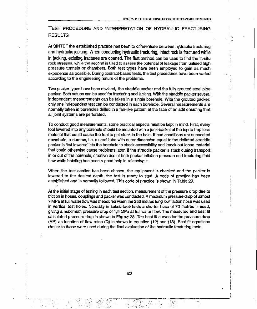
HYDRAULIC FRACTURING ROCK STRESS MEASUREMENTS
Test procedure and interpretation of hydraulic fracturing
RESULTS
At SINTEF the established practice has been to differentiate between hydraulic fracturing and hydraulic jacking. When conducting hydraulic fracturing, intact rock is fractured while in jacking, existing fractures are opened. The first method can be used to find the in-situ rock stresses, while the second is used to assess the potential of leakage from unlined high pressure tunnels or chambers. Both test types have been employed to gain as much experience as possible. During contract-based tests, the test procedures have been varied according to the engineering nature of the problems.
Two packer types have been devised, the straddle packer and the fully grouted steel pipe packer. Both setups can be used for fracturing and jacking. With the straddle packer several independent measurements can be taken in a single borehole. With the grouted packer, only one independent test can be conducted in each borehole. Several measurements are normally taken in boreholes drilled in a fan-like pattern at the face of an adit ensuring that all joint systems are perforated.
To conduct good measurements, some practical aspects must be kept in mind. First, every tool lowered into any borehole should be mounted with a junk-basket at the top to trap lose material that could cause the tool to get stuck in the hole. If bad conditions are suspected downhole, a dummy, i.e. a steel tube with outer dimension equal to the deflated straddle packer is first lowered into the borehole to check accessibility and knock out loose material that could otherwise cause problems later. If the straddle packer is stuck during transport in or out of the borehole, creative use of both packer inflation pressure and fracturing fluid flow while hoisting has been a good help in releasing it.
When the test section has been chosen, the equipment is checked and the packer is lowered to the desired depth, the test is ready to start. A code of practice has been established and is normally followed. This code of practice is shown in Table 29.
At the initial stage of testing in each test section, measurement of the pressure drop due to friction in hoses, couplings and packer was conducted. A maximum pressure drop of almost 7 MPa at full water flow was measured when the 250 metres long low friction hose was used in vertical test holes. Normally in subsurface tests a shorter hose of 70 metres is used, giving a maximum pressure drop of 1,5 MPa at full water flow. The measured and best fit calculated pressure drop is shown in Figure 73. The best fit curves for the pressure drop (AP) as function of flow rates (Q) is shown in equation (12) and (13). Best fit equations similar to these were used during the final evaluation of the hydraulic fracturing tests.
103

HYDRAULIC FRACTURING ROCK STRESS MEASUREMENTS
Table 29 Code of practice for hydraulic fracturing.
1 Start the data logging computer, and establish zero level for all gauges.2 Do frictional pressure loss calibrations.3 Increase packer pressure until just below anticipated shut-in pressure.4 Increase injection pressure to one third of packer pressure.5 Monitor pressure gauges for any pressure drop indicating leakages.6 ■ Decrease injection pressure to zero.7 Increase injection pressure at a rate such that fracturing / jacking is accomplished in 5 -
0 minutes (higher pressure, takes longer time).8 Keep the water flowing into the test section as short time as possible, but until a
constant flow rate has been established.9 Close the shut off valve and monitor the injection pressure decay.10 Open bleed off valve and let the section bleed off.11 Repeat step 7 to 10 once.12 Activate the check valve in injection flow line.13 . Repeat step seven to eight.14 Decrease injection pressure at the same rate as it was increased.15 Monitor pressure decay after the check valve has closed.16 Repeat step 13 to 15 once.17 Bleed off injection pressure and deflate the straddle packer, pull out of hole.18 Make an oriented imprint of the test section.19 Before equipment is taken off location a quality check of the registered data is
conducted to ensure good measurements. If bad results are found, more testing is needed.
O dP(250m)--------dPt(250m)
O dP(70m)
......... dPt(70m)
WATER FLOW [l/min]
Figure 73 Measured and calculated best fit pressure drop in splitting hoses. The 70 metres hose is a standard 4-layer hydraulic hose, while the 250 metres hose is a low friction high strength 2-layer hydraulic hose.
104
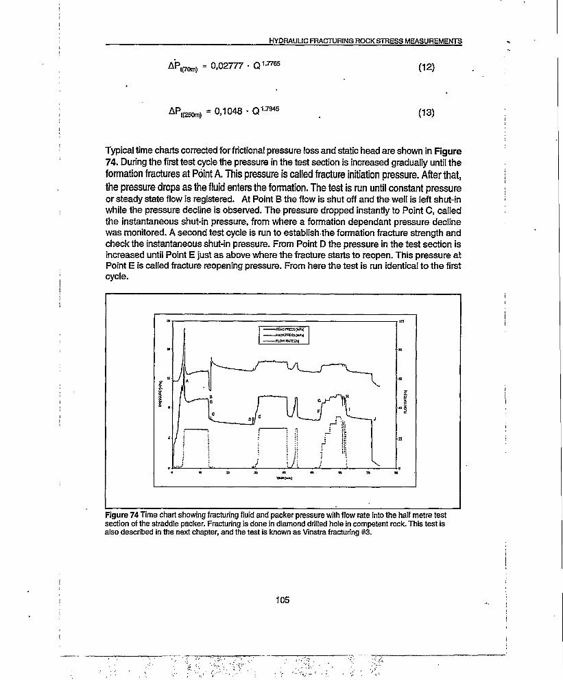
HYDRAULIC FRACTURING ROCK STRESS MEASUREMENTS
APt{70m) = 0,02777 • Q17765 (12)
AP«250m) = 0,1048 • Q1:7945 (13)
Typical time charts corrected for frictional pressure loss and static head are shown in Figure 74. During the first test cycle the pressure in the test section is increased gradually until the formation fractures at Point A. This pressure is called fracture initiation pressure. After that, the pressure drops as the fluid enters the formation. The test is run until constant pressure or steady state flow is registered. At Point B the flow is shut off and the well is left shut-in while the pressure decline is observed. The pressure dropped instantly to Point C, called the instantaneous shut-in pressure, from where a formation dependant pressure decline was monitored. A second test cycle is run to establish the formation fracture strength and check the instantaneous shut-in pressure. From Point D the pressure in the test section is increased until Point E just as above where the fracture starts to reopen. This pressure at Point E is called fracture reopening pressure. From here the test is run identical to the first cycle.
—PACXPfiESSIKPjJ
.-FWRMEM
Figure 74 Time chart showing fracturing fluid and packer pressure with flow rate into the half metre test section of the straddle packer. Fracturing is done in diamond drilled hole in competent rock. This test is also described in the next chapter, and the test is known as Vinstra fracturing #3.
105

HYDRAULIC FRACTURING ROCK STRESS MEASUREMENTS
In the fourth test cycle the pressure in the test section is increased to Point F where the fracture opens. The pressure in the test section is governed by the flow rate, and from Point G the pressure is increased in stages until a maximum flow rate is reached. At each step fluid is injected until a steady state flow is observed. From Point H the pressure was reduced gradually until the check valve closed. At this Point I, called the fracture closure pressure, the fracture does not take any more water and equilibrium between the pressure in the test section and the stresses normal to the fracture was obtained. From this point the test section was left closed in and the pressure decline monitored. At Point J the test was finished, and the pressures bled off from the test section.
The flow rate time chart shows how the flow rate is related to pressure variation. As it is shown above, the equipment is set up to let the fluid flow be directly governed by the pressure in the test section. A maximum flow rate is set by the pump, but the actual flow rate is governed by the pressure regulation and the hole conditions. The packer pressure is also monitored during the test, and in the figure a pressure increase is seen just after the instantaneous shut-in pressure at Point C. At this stage of testing, the operator suspected leakage in the packer circuit and increased the packer pressure to prevent leakage from the test section. Additionally, several test cycles may be run to find opening, reopening and closing pressures of existing or induced fractures. Variations in sequence pressurisation may also be run to assess the leak-off characteristics after fracturing. Consequently this part of the test program can be run in both jacking and fracturing operations.
When test section pressure is plotted versus fluid flow rate for each test cycle the characteristic pressures can easily be found. These curves are shown in figures Figure 75 to Figure 78. In the first test cycle the pressure is increased with virtually no change in theflow rate until the rock is fractured at approximately 11 Mpa pressure. Then the pressure drops as the fracture opens but increases until the maximum preset flow rate is reached, from where it drops to a level balancing the stress acting on the fracture. Pumping is continued and the pressure in the test section increases slowly as a reservoir is created in the fractures continuously growing. Closing the water flow by shutting in the test section, almost instantaneously reduces the test section pressure, and the instantaneous shut-in pressure is found. Gradually the pressure in the test section decreases, suggesting that small amounts of water enter the rock.
The pressure versus flow rate graphs from subsequent tests in test section 3 at Vinstra (see figue 1) all show similar relationships. Test cycle number 2 and 3 show instantaneous shut-in pressures, while number 4 has a gradual pressure decline to allow the closure pressure of the fracture to be observed. An initial nonlinear pressure versus flow relation is always seen, which is caused by initial reopening of the fracture followed by a flow dependant pressure increase. Whether the test section is shut-in instantaneously, or pressure is reduced gradually allowing the check valve to shut-in the section, the interpreted pressures almost equal each other. Thus, the instantaneous shut-in pressure equals the closure pressure. In a low stress area with more fractures, however, the pressure-decrease after shut-in of the section would be substantial, and render the interpretation more difficult.
106

HYDRAULIC FRACTURING ROCK STRESS MEASUREMENTS
g. 1440
540 1040 1540 2040 2540 3040 3540 4040FLOW RATE (Umin)
Figure 75 Pressure plotted versus flow into test section for the first test cycle at the Vinstra test no.3
5 12.00
■ 0.00 10.00 15.00 20.00 25.00 30.00 35.00 40.00FLOW RATE (l/rnin)
Figure 76 Pressure plotted versus flow into test section for the second test cycle at the Vinstra test no.3
107

HYDRAULIC FRACTURING ROCK STRESS MEASUREMENTS
14.00
35.00 40.0010.00 15.00 20.00 25.00 30.00FLOW RATE (l/min)
Figure 77 Pressure plotted versus flow into test section for the fourth test cycle at the Vinstra test no.3
14.00E 12.00
$ 10.00
10.00 15.00 20.00 25.00 30.00 35.00 40.00FLOW RATE (l/min)
Figure 78 Pressure plotted versus flow into test section for the third test cycle at the Vinstra test no.3
108

HYDRAULIC FRACTURING ROCK STRESS MEASUREMENTS
Evaluating pressures from the time charts are not sufficient to evaluate the stresses as shown above. A more precise way of determining the characteristic pressures from a fracturing test must be done. Thus, each test cycle is shown as pressure versus flow rate charts. This chart type is produced to define the characteristic opening and closing pressures of the fracture. Due to the sometimes subtle changes in curvature, extracting exact pressure readings may be difficult. This can be overcome if the tangents to the different sloped segments of the curve are traced, and the value given at the point of intersection.
When the plane of fracturing is nearly parallel to the drill hole, the equations developed by Hubbert and Willis [90] may be used to calculate the principal effective stress components. If the fracture plane is oriented at an angle to the drill hole, a technique such as the method of hydraulic testing of preexisting fractures (HTPF), Comet [91] may be applied. This method has not been used in the evaluation of the data presented here. Other interpretation techniques have also been proposed including a fracture mechanic approach, Baumgartner [92] and Rummel [93], and poroelastic approaches applied when tests are run in porous media, Detoumay et al. [94].
min = Ps " P0 (14)
■T + 3PS - Pf - P0 (15)
:=3PS-Pr-P0 (16)
T = p, - pr (17)
T = Pf - Pc (18)
T - P, " Ps (19)
where:PcPoP,T
Effective maximum tangential stress Fracture closure pressure Measured pore pressure Fracture reopening pressure Formation fracture strength
o’n* Effective minimum tangential stressP, Fracture initiation pressurePp Fracture propagation pressurePs Instantaneous shut-in pressure
109

HYDRAULIC FRACTURING ROCK STRESS MEASUREMENTS
In this context where it is only dealt with relative impermeable rock types, the first approach given by the Hubbert and Willis' equations (equation (14) and (15)) has been employed. Equation (15) is valid for the first test cycle, but the formation fracture strength must be known. Equation (16) is applicable for subsequent tests provided equation (17) is valid and thus make equation (15) redundant. The formation fracture strength is not equal to the tensile strength of the formation measured in the laboratory. From the hydraulic testing presented here, considerable scatter is inherent in the results. The formation fracture strength can therefore be approxiated from any of the equations (17), (18) or (19). Equation (17) is preferred because it has shown to be virtually independent of the flow rate or any other test variables, and considers only fracture initiation and reopening pressure. The results based on these equations are not biased by assumptions on various fracture models and choice of input parameters made in a forward modelling approach. Thus, they represent mechanisms in the rock without any anticipations on for example fracture mechanical models and readjusted stress fields near the closed fracture.
Casing and cement integrity - formation integrity tests
The integrity of the total lining is very important during drilling of petroleum wells. During all operations in the well it is required to have at least two working safety barriers in case high pressure conditions are encountered or if one safety barrier is destroyed. An intact (over-) balanced mud column in the well is regarded as one safety barrier while a working christmas-tree with properly cemented liner is the other.
After each casing string is cemented in place and after drilling some metres into the formation below the casing seat, a pressure test called the formation integrity test (FIT) is run to verify the integrity of the casing, the cured cement and formations surrounding the casing seat. This is done to verify that the wellbore can withstand the mud pressure required to drill safely to the next depth at which casing will be set. The test is compulsory and prescribed by the Norwegian Petroleum Directorate (NPD) due to safety regulations.
Before any analysis of the formation integrity test results is done, it must be emphasized that these tests are primarily done to test the casing shoe integrity. Additionally, it must be noted that the casing shoe is always set in a formation supposed to be the most competent and strongest. Furthermore, the set points for the casing shoes are based on a compromise between safety considerations, drilling mechanics and well path objectives. Therefore, when data from formation integrity tests are analysed in a geomechanical context, the input data are not randomly chosen, a bias to competent, stiff and thus possible high stress areas ispreferred.
A leak-off test is normally conducted using the cement pumps with typical pumping rates of 40 - 250 l/min, and the total volume of fluid involved are normally some thousand litres. Higher rates are used if large open hole sections are tested. Nevertheless, pumping rates during the tests are normally kept low to avoid frictional pressure loss. During the test, the annulus valve is shut and the pressure buildup on the rig floor is measured. The test fluid
110

is the drilling mud. Contrary to the measurements described in the preceding chapter, the pumping rate is kept constant throughout the test cycle. Because of the pumped mud volume, the increasing pressure is continuously recorded. Today, standard recording sheets are used where the pressure is recorded every minute.
According to how the tests are conducted, various names are applied to them. A typical pressure versus volume and consecutive pressure versus time relationship for an extended leak-off test (ELOT) conducted in a short open hole section is shown in Figure 79. In the start, a constant pressure increase for each incremental drilling fluid volume is recorded showing that the early test results fall on a straight line. The straight line trend continues until Point A, where the formation starts to take whole mud. The pressure at Point A being called the leak-off pressure is used to calculate the formation fracture gradient. Pumping is continued to ensure that the fracturing pressure has been reached and further until the pressure subsequently drops, showing that the fracture opens. The fracturing pressure means the maximum pressure in the test section during testing. At Point B, the pump is stopped, and the well is left shut-in to observe the rate of pressure decline. The rate of pressure decline shows the rate at which mud is being lost to the formation. Sometimes the annular valve is opened and the amount of returned mud is recorded. To be considered a true ELOT, the test cycle should be repeated several times to establish a reliable leak-off pressure. The FIT may be run to any level of completeness (1 - 4) as shown in Table 30.
HYDRAULIC FRACTURING ROCK STRESS MEASUREMENTS
VOLUME PUMPEDFigure 79 Typical pressure versus volume and subsequent pressure versus time chart for an extended leak-off test conducted in a short open hole section. The minimum volume line represents nominal expansion of tubular goods due to pressure increase. Since more fluid are needed, this may be caused by either a leak or the tested formation taking whole mud during testing.
111

HYDRAULIC FRACTURING ROCK STRESS MEASUREMENTS
Table 30 Different levels of completeness of formation integrity tests (FIT).
1 Formation Integrity Test (FIT): The test is run until actual maximum mud weight is exceeded, ■or until somewhere along the line OA.
2 Leak-off Test (LOT): The test is run beyond Point A, and proper leak-off pressure is determined.
3 Leak-off Test (LOT): The test is ran beyond Point B, and formation breakdown pressure is determined additionally.
4 Extended Leak-off Test (ELOT): The well is shut-in at Point B, and the pressure decline is monitored, which may give an indication on the instantaneous shut-in pressure. A second and perhaps a third repressurization and subsequent shut-in may be performed.
While drilling and completing petroleum wells, formation integrity tests (FIT) are usually run and recorded after every casing is cemented. Test values obtained during drilling are always given in the final well report by Norwegian operators. Sometimes it is stated whether the
. data come from FIT, LOT or ELOT and often the actual pressure versus volume and time graphs are included. However, some operators do not conduct these tests if they are drilling in what is termed “known formations”, or in areas that is previously drilled. Other operators conduct limit tests, but do not record the results if they are satisfactory from a drilling point of view. If the tests are recorded, they are sometimes misleading for stress evaluations since different or unknown test procedures may have been applied for each test. Therefore, each recorded curve must be investigated and related to other information on drilling and lithology before the test results are used for any stress evaluation.
Another issue encountered during the actual tests is that the driller and the responsible drilling engineer do not deliberately want to damage the new section into which they are drilling. They will avoid all kinds of operations in the well that may lead to possible future wellbore stability problems. Therefore the test section is often pressurized until anticipated maximum mud pressure for the next section is exceeded. If no leak-off is reported, they will go on to drill the next section as planned. Data retrieved from this kind of tests (FIT) is of limited value for any rock mechanical evaluation. They only suggest that the formations are subjected to a higher than recorded, but unknown minor principal stress.
In Norsk Hydro it has become an established practice to conduct micro-frac tests in all tested exploration wells that are permanently abandoned. The regular procedure is to run leak-off tests slightly beyond Point A in Figure 79. Sometimes only formation integrity tests are conducted at each casing shoe in the wells. Stress profiling is never done, and extended leak-off tests have been ended since the early nineties. Then, extended leak-off tests were requested in a vertical well to explore indications of high horizontal stresses exceeding the vertical overburden stress. The initial pressure buildup was done according to the prescribed plan. Nevertheless, the test was stopped by the drilling engineer during the first test cycle because leak-off to the formation was registered after formation breakdown pressure was reached. Furthermore, a pressure decrease was reported after shut-in of the well and mud bleed-back was reported after opening of the annulus valves. Finally chunks of virgin formation and cement were reported on the shale shakers when drilling into the new section commenced. The boulders were taken as proof of the extended leak-off test’s detrimental effect to wellbore stability. Consequently, extended leak-off tests have hardly
112

HYDRAULIC FRACTURING ROCK STRESS MEASUREMENTS
ever been conducted later. In retrospect, the personnel involved with the well apparently was not aware of how an extended leak-off test works. They did not seem to know the effect it had on the well and what the wellbore looked like when it was drilled. This was probably the only mistake made during the operation. If borehole televiewer images had been available, fracture traces from the extended leak-off test would presumably have been visible in the wellbore, arid furthermore the images would also have revealed drilling induced fractures and natural fractures.
Another likely explanation of the problems that were experienced while drilling into the new formations below the casing shoe, may be loss of hydraulic pressure support in the rathole after the casing shoe cement cured. The rathole is the part of the wellbore between the cemented liner and the target depth appearing without cement in Figure 80. After the cement has cured, it is efficiently sealed from hydraulic contact with the rest of the mud column. If any mud in the rat hole leaks off to the surrounding formations, the pressure will equilibrate to the formation pore pressure and overbalance is lost, increasing the tangential stresses perhaps beyond failure. Massive spalling may commence in the rat hole, resulting in major problems when the casing shoe is drilled out. Hole cleaning problems with resulting pack off might also have been the principal problem. This is caused by wellboreenlargement reducing the mud return velocity, which in turn reduces lift capacity. In the paragraphs below it is shown that the long rathole did not have any adverse effects on the stability at the 12 1/4“ casing shoe of the Visund 34/8-1 OS well.
Frames shown in following figures
Formation .Casing .Cement Casing shoe Rat hole
.TD wider wellbore
Conical wellbore due to vibration
Narrower wellbore
Figure 80 Schematic illustration of cemented casing, drilled through casing shoe and rat hole. Frames indicating the Formation Micro Imager captions in the next three figures are also shown by dashed rectangles indicating cement at casing shoe and upper part of rat hole (121/4"), lower part of rat hole and wellbore (81/2"). The cement plug in the casing shoe was approximate 50 metres long with a rat hole of 12 metres. TD refers to target depth.
At the 121/4“ casing shoe in the Visund 34/8-1 OS well, the cement plug was approximately 50 metres long with a rat hole of 12 metres according to Formation Micro Imager (FMI) logs. In this well the FMI tool was run before the next casing was installed and cemented in place.
113

HYDRAULIC FRACTURING ROCK STRESS MEASUREMENTS
In Figure 80 the casing shoe and rat hole in the lower part of the 12 1/4” section is sketched. After the well is drilled to target depth, it is cleaned by pumping high viscous pills and circulating drill mud until the contents of the return flow equals the input flow. Irrespectively of clean up operations, some sag will occur in the mud column causing solids and cuttings to accumulate at the bottom. If the liner is not very close to the wellbore bottom, the cement returning up the annulus will not displace the debris accumulated here. When the casing shoe is drilled out, the debris will be circulated up with cuttings from underneath the cement, and will show up on the caliper log like an enlargement as in Figure 80.
In the Visund 34/8-1 OS well, the casing shoe was drilled out at a depth of 2555,5 metres with a rat hole extending almost 12 metres further down. The casing shoe and rat hole in the first FMI image in Figure 81 are shown with the tensile fracture created by an extended leak-off test that resulted in a leak-off pressure of 48 MPa (1.88 g/cm3 equivalent mud
weight). The vertical fracture suggests a horizontal minor principal stress oriented NNE - SSW. Towards the bottom of the rat hole the fracture branches out in an oblique angle to the borehole and fades away before the 121/4“ target depth.
In the next FMI caption in Figure 82 towards the lower part of the rat hole, the signature of the signals changes as the 8 1/2” section is approached. This can be caused by a lithology change or is perhaps due to different open hole time or different bits used. There may also have been cement in place, but it has fallen out during drilling due to mediocre quality. Below target depth a conical transformation from 121/4 “to 81/2“ is picked up by the FMI caliper. At least two explanations can be given for this. The drill bit has either whirled considerably at the bottom of the rathole while tracking the nominal wellbore diameter further down, or when the 8 1/2” drill bit engaged the formation, stress concentrations resulted in spalling, or both.
The last FMI image some 90-metres deeper in the well reveals that tensile fractures are formed in the wellbore due to normal operation in the well as shown in Figure 83. Although no leak-off test has been conducted, fractures have been created. The most likely explanation for this is a combination of stress perturbation due to the wellbore itself, pack off and surge and swab caused by operations in the well. This implies that operations in the well can induce fractures that are not critical to the long time stability of the well itself. Normally the presence of these fractures will only be observed when the wellbores are investigated by some kind of televiewer.
114

HYDRAULIC FRACTURING ROCK STRESS MEASUREMENTS
Figure 81 Formation Micro Imager image of fractures caused by the leak-off test at the 121/4“ casing shoe in well 34/8-1 OS. The image shows fractures running through rat hole and cement. The vertical blue line in the image show way up in the borehole while the left hand portion of the figure shows caliper and orientation data.
115
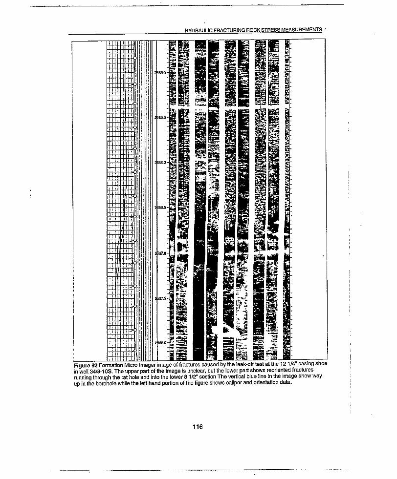
HYDRAULIC FRACTURING ROCK STRESS MEASUREMENTS •
Figure 82 Formation Micro Imager image of fractures caused by the leak-off test at the 121/4" casing shoe in well 34/8-1 OS. The upper part of the image is unclear, but the lower part shows reoriented fractures running through the rat hole and into the lower 81/2" section The vertical blue line in the image show way up in the borehole while the left hand portion of the figure shows caliper and orientation data.
116

HYDRAULIC FRACTURING ROCK STRESS MEASUREMENTS
Figure 83 Formation Micro Imager image of fractures caused by operations some 90 metres below the former figure in the 81/2“ section in well 34/8-1 OS. Both vertical and en echelon fractures are visible. The vertical blue line in the image show way up in the borehole while the left hand portion of the figure shows caliper and orientation data. The well is now deviated from the vertical and borehole elongation is observed.
117

HYDRAULIC FRACTURING ROCK STRESS MEASUREMENTS
Figure 84 Formation Micro Scanner images from 3065 - 3068 metres and 3083 - 3085 metres depth
showing induced fractures in the well 7316/5-1. Both sub-vertical and en echelon fractures can be seen in the two images. The well is almost vertical and azimuthal information is given above the image. The caliper
data in the left part indicates some elongation of the borehole.
118

HYDRAULIC FRACTURING ROCK STRESS MEASUREMENTS
Figure 85 Formation Micro Scanner images from 3140 - 3143 metres and 3225 - 3228 metres depth showing induced fractures in the well 7316/5-1. Sub-vertical and perhaps en echelon fractures can be seen in the two images. The well is almost vertical. The caliper data in the left part indicates varying degree of elongation of the borehole.
119

HYDRAULIC FRACTURING ROCK STRESS MEASUREMENTS
1000
4000
5500
6000
_____________________ Equivalent circulation density specific gravity (g/cm3)____________________________Figure 86 Norsk Hydro results from formation integrity tests and leak-off tests taken at casing set points and drawn versus depth. Values are presented as equivalent circulation density specific gravity measured topside on drilling platform.
120

HYDRAULIC FRACTURING ROCK STRESS MEASUREMENTS
While searching for drilling induced fractures in petroleum wells, Formation Micro Scanner data (FMS) run in wells from the Barents Sea have been explored. Figure 84 and Figure 85 show images from four intervals in the vertical well 7316/5-1. Changes in resistivity in the formations represent lithological changes and are shown in the images illustrating bedding planes. Furthermore, fractures oriented en echelon and parallel to the wellbore are seen. Similar fractures are found in the rest of the logged well, but neither stability problemsrelated to the fractures nor cave-ins are identified. In retrospective, the well has been drilled with a suitable balanced mud with respect to chemistry and weight. During operations, pressure surges or temperature effects must have caused the wellbore fluid pressure to exceed the tangential stresses and the formation tensile failure strength, and have created the fractures.
All images shown in Figure 83 to Figure 85 show wellbores with fractures likely to be induced by drilling operations. The induced fractures are the results of combinations of unfavourable wellbore orientation, drilling mud, lithology, mechanical properties and stresses. These fractures .appear similar to the fractures created during the leak-off tests shown in Figure 81 and Figure 82. The induced fractures can more specifically be caused by:
Stress perturbation due to the well itself may lead to tensile fractures or breakouts. Over- and underbalanced drilling can lead to either tensile fractures or cave-in in the well respectively.Surge and swab during tripping can like a pack-off while drilling lead to hydraulic fracturing and create tensile fractures in parts of the well.Cooling the mud may reduce the tangential stresses and thus favour tensile fracturing.
Fractures generated by hydraulic fracturing are observed from image logs in several wells. In these wells, however, no references to any kind of problems have been given in the daily drilling reports. It is therefore unlikely that they have had any adverse effects on wellbore stability. They only add to the already existing fracture network surrounding the well and may accumulate some drilling mud. This can be seen if the drilling mud return is carefully monitored. After the mud pumps have been shut off, the well will bleed back considerable amounts of drilling mud, where the volume will be characteristic of the fracture network surrounding the well.
Assessment of stresses from Leak-off Tests
The leak-off test provides a cost-effective method to get better knowledge of the minor principal stress. Many subsurface evaluation tasks use this information, and should justify any additional fractures in the relative strong formations surrounding the casing shoes. Test results from the Norwegian Continental Shelf done before 1992 by Norsk Hydro are plotted versus depth in Figure 86. Variation in the measuring results reported as leak-off tests implies some scattering features. The data set comprise measuring values from different
121

HYDRAULIC FRACTURING ROCK STRESS MEASUREMENTS
test types: formation integrity tests (FIT), leak-off tests (LOT) and extended leak-off tests (ELOT). Data points representing mud weights (MW) of 1.5, 1.6 and 1.8 g/cm3 are not representative for their respective formation strength at their given depths. These results are likely tests run to exceed the chosen mild weight,, i.e. FIT. Therefore they only show that the formation break down pressure is higher, and should be omitted from this kind of plot. Geographical and lithological variations are also likely to influence on the scatter in Figure 86. Another factor that also induces the scatter, however more difficult to assess, is the different operational practices during testing.
Research work conducted by Shell and reported by Breckels and van Eeckelen [95], on stresses from the Mexican Gulf Coast, Brunei, Venezuela and the North Sea, showed clear trends of the minor principal stress magnitude versus depth. This relationship is regularly used in the assessment of rock stresses in unmapped areas. When they compare leak-off values to be approximate 11 percent higher than the instantaneous shut-in pressure from hydraulic fracturing, they attribute this to the fact that the leak-off test values are not corrected for stress concentrations due to the borehole itself. In other words they interpret the leak-off test to predict too high minor principal stresses. They also propose ideas on how abnormal pore pressures affect the minor horizontal stress. Their general opinion of the minor horizontal stress in normal consolidated, tectonic inactive sedimentary basins is shown in equation (20) and (21).
= 0.0053h1-145 + 0.46(Pm-P0), for h 2 3500m (20)
= 0.0264h - 31.7 + 0.46(Pm-P0), for h > 350C (21)
Where: ohmin: Minor principal stress h: OverburdenPm: Measured pore pressure P0: Normal pore pressure
Unpublished results from the Snorre oil field operated by Saga Petroleum show consistent values of both the major and minor horizontal stresses based on interpretation of leak-off values. According to R.K. Bratli (pers.comm.), reports from this oil field give trend lines for the two horizontal stresses (ohmin, q^) described by equation (22) and (23) from observations down to 3.600 metres depth. The reported deviations from these regression lines are in the order of 3 percent. The two horizontal stresses are obtained by inversion of LOT values from deviated boreholes as described by Aadnoy [96].
122

HYDRAULIC FRACTURING ROCK STRESS MEASUREMENTS
°hmax = 0-023h + 1.8 , for h s 3600m (22)
CThmin = 0.020h + 0.5 , for h s 3600 m (23)
Caillet et.al.[97] report on stress orientation in the Lille Frigg area. They show that the minor principal stress determined from LOT are in the order of 90 percent of the overburden stress determined by integration of the density logs. They use an upper envelope to the LOT values as an interpretation line for the minor principal stress as opposed to a lower envelope favoured by most others. Thus, the technique gives different results, and furthermore seems too high. Interpretation of their data is shown in equation 25 as an estimate of the minor principal stress in the area.
omln = 0.0172 • h - 3.75 for h < 4500m (24)
Based exclusively on ELOT values Lena [98] reports a relationship for the minor principal stress from the overburden in Ekofisk field given in equation (25). Here the average ratio of the minimum horizontal stress to the overburden stress is 0.92. Although farther to the south and in the Central Graben, relationships similar to the results found in the Frigg and Oseberg areas were displayed here.
omin = 0,0185 • h - 2 MPa for 500 s h <; 2900m (25)
Both ELOT and LOT values collected from the Oseberg field have been studied. Out of some 130 digitized and reevaluated test reports, only 34 have been found suitable for interpretation of the minor principal stress by Amundsen and Teufel (pers.comm.) and reported by Amundsen [99]. They report the minor principal stress to vary according to depth as shown in equation (26).
omin = 0.017 • h - 1.09 MPa for h s 3500m (26)
The various estimates of the minor principal stresses shown above and based on reliable ELOT and LOT data are plotted as gradients versus depth in Figure 87. The differences in the minor principal stress assessment are probably caused by various geological setting and possibly also to the interpretation and calculation methods used.
123

HYDRAULIC FRACTURING ROCK STRESS MEASUREMENTS
Equivalent mud weight (g/cm3)
1 1.5 2 2,5 3
B Frigg
* Visund
+ Snorre H
X Snorre h
Figure 87 Estimated minor principal stresses from several North Sea petroleum fields plotted as gradients (specific weight or equivalent mud weight) versus depth. Data from the Visund field are presented in the next chapter, but given here as reference. Data from the Snorre field show results from inversion of the LOT values, and gives the minor and major horizontal stresses, Snorre h and Snorre H respectively . Data from the cited authors are plotted together with the widely used Breckels and van Eekcelen (op.cit.)minor principal stress criterion as reference, marked B&vE.
Recommended practice for conducting (Extended) Leak-off
Tests
Most of the reported extended leak-off test values (ELOT) have been collected to find fracture gradients or safe mud weights, not to assess the minor principal stress value. To use the test results in stress determinations, some guidelines or code of practice should be followed. Whether a full extended leak-off test is done or a reduced test of some sort, the basic principles outlined in Table 31 should be followed. The code of practice is based the knowledge acquired from evaluating leak-off tests, the procedures for extended leak-off tests presented by Knapstad [100] and Kunze and Steiger [10i]. When (E)LOT values are collated to form a minor principal stress prognosis, a quality measure should also be assigned to the values. This qualifier should be used to separate properly executed tests from the abundant poor tests, and thus keep a high standard on the stress evaluation. The qualifier should furthermore be based on the completeness of the tests and the way pressure data are obtained. The proposed way of doing this is shown in Table 32. In stress evaluations, data of quality A and B should preferably be used. The low quality groups D, E and F should not be used unless special care is exercised in the evaluation.
124
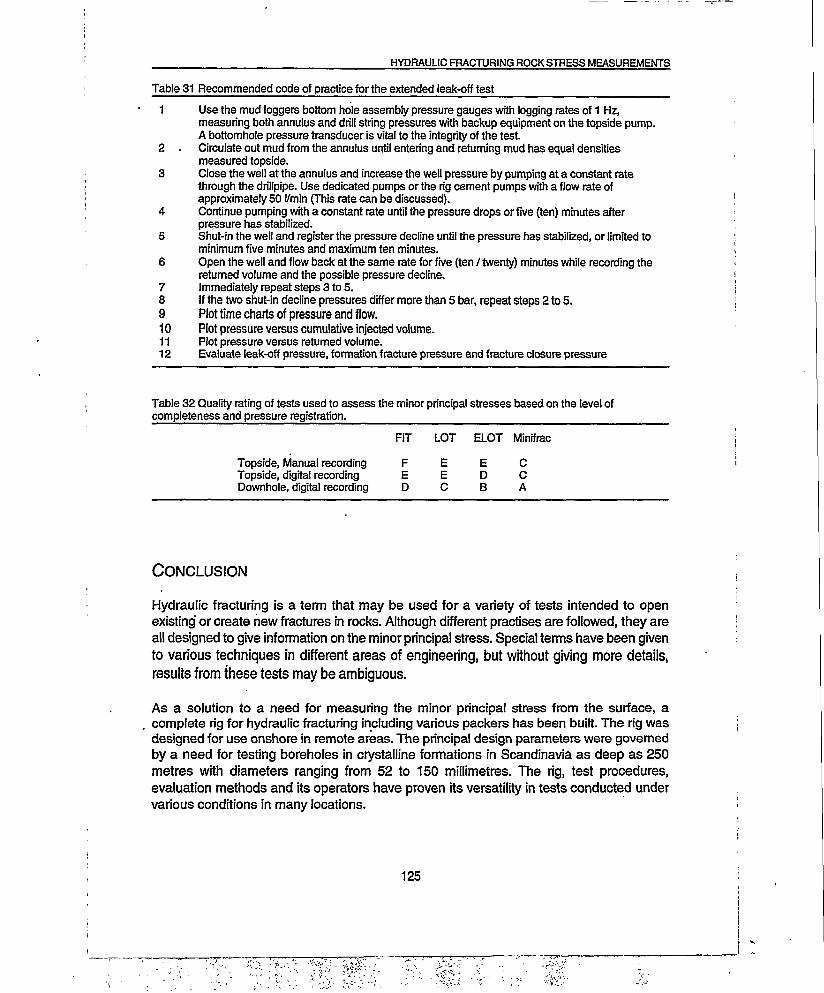
HYDRAULIC FRACTURING ROCK STRESS MEASUREMENTS
Table 31 Recommended code of practice for the extended leak-off test
1 Use the mud loggers bottom hole assembly pressure gauges with logging rates of 1 Hz, measuring both annulus and drill string pressures with backup equipment on the topside pump. A bottomhole pressure transducer is vital to the integrity of the test.
2 . Circulate out mud from the annulus until entering and returning mud has equal densitiesmeasured topside.
3 Close the well at the annulus and increase the well pressure by pumping at a constant rate through the drillpipe. Use dedicated pumps or the rig cement pumps with a flow rate of approximately 50 l/min (This rate can be discussed).
4 Continue pumping with a constant rate until the pressure drops or five (ten) minutes after pressure has stabilized.
5 Shut-in the well and register the pressure decline until the pressure has stabilized, or limited to minimum five minutes and maximum ten minutes.
6 Open the well and flow back at the same rate for five (ten / twenty) minutes while recording the returned volume and the possible pressure decline.
7 Immediately repeat steps 3 to 5.8 If the two shut-in decline pressures differ more than 5 bar, repeat steps 2 to 5.9 Plot time charts of pressure and flow.10 Plot pressure versus cumulative injected volume.11 Plot pressure versus returned volume.12 Evaluate leak-off pressure, formation fracture pressure and fracture closure pressure
Table 32 Quality rating of tests used to assess the minor principal stresses based on the level of completeness and pressure registration.
Topside, Manual recording
FIT
F
LOT
E
ELOT
E
Minifrac
CTopside, digital recording E E D CDownhole, digital recording D C B A
Conclusion
Hydraulic fracturing is a term that may be used for a variety of tests intended to open existing or create new fractures in rocks. Although different practises are followed, they are all designed to give information on the minor principal stress. Special terms have been given to various techniques in different areas of engineering, but without giving more details, results from these tests may be ambiguous.
As a solution to a need for measuring the minor principal stress from the surface, a complete rig for hydraulic fracturing including various packers has been built. The rig was designed for use onshore in remote areas. The principal design parameters were governed by a need for testing boreholes in crystalline formations in Scandinavia as deep as 250 metres with diameters ranging from 52 to 150 millimetres. The rig, test procedures, evaluation methods and its operators have proven its versatility in tests conducted under various conditions in many locations.
125

HYDRAULIC FRACTURING ROCK STRESS MEASUREMENTS
The bulk of available stress .data in petroleum engineering is found in the shales in the overburden where the casing shoes are set. At each casing shoe a formation integrity test of some kind is conducted. The formation integrity test procedure is subjected to individual interpretations and individual reporting of the test results. The reported values must therefore be quality checked before they are used in rock mechanic evaluations. Additionally, it must be acknowledged that the casing shoe is always set in the strongest possible formation available for its purpose. Thus, the measured stresses are biased since stronger formations are normally stiffer and therefore accommodate higher stresses.
Some thirty out of 130 tests could be used in a regional stress study in the Oseberg field. Due to various interpretation techniques among operators, stress results of different quality and completeness are presented from petroleum fields. If the formation integrity tests shall be used to predict part of the stress tensor, increased credibility must be invested in both measuring and interpretation techniques. The only way to do this, is to advocate the use of standards since no common code of practice or standard exists right now. Such a code of practice with a quality rating scheme is proposed as a starting point to standardize the testing. When good measurements are conducted, the interpretation of the results will be relative straightforward.
126

MORPHOLOGICAL ROCK STRESS INDICATORS
MORPHOLOGICAL ROCK STRESS INDICATORS RELATED TO
ROCK STRESS MEASUREMENTS AND TUNNEL SPALLING
OBSERVATIONS
In underground openings a qualitative appraisal of stress intensity compared with rock strength is possible by mapping the occurrence of spalling. This technique gives the best results in hard rocks with low or no time dependant stress relaxation, or in formations where spalling is most apparent. A similar observation technique may be employed to assess stresses in areas with no soil cover or especially in valley sides. In such areas, surface mapping or registration of exfoliation intensity may suggest the maximum stress orientation in the rock, and to a lesser degree the relative magnitude of the stresses. Such mapping was conducted in the Kobbelv area in the county of Nordland. Here a program consisting of rock stress measurements, rock strength testing and some tunnel mapping was devised to explore if varying exfoliation intensity could be related to subsurface stress distributions.
Bungum et al. (op. cit.) have reviewed the earthquake locations for the period 1955 - 1989 as reported from several agencies. One area of increased activity extends both on - and offshore the northern part of the county of Nordland. Their rose diagram of the axis of maximum compression in this area is oriented WNW - ESE which coincides with the axis of the major principal rock stress measured by Hanssen and Myrvang [102]. In the present study these data were reinterpreted by use of the computer code DISO.
During construction of the Kobbelv hydropower scheme, the Norwegian State Power Board (NVE) experienced both immediate and time dependant spalling in their tunnels. They observed that spalling was more intense in shallow tunnels in northerly directions than in tunnels at depth and in other direction. They seldom observed any spalling immediately after blasting, but if no support were installed, severe spalling started after advancing some rounds. Similar problems were also experienced during construction of the Kobbskar highway tunnel in the same area according to Pegg [103]. One year after commissioning, the highway tunnel had to be partly closed to scale and bolt substantial parts. At the time of construction, however, no measures were taken against heavy spalling. Therefore, when the rock stress measurements and the exfoliation observations commenced a priori indications of an anomalous stress distribution in the area already existed.
127

MORPHOLOGICAL ROCK STRESS INDICATORS
Reinoksvatne.t
ReinoksvatnetLitletindvatnet
Kobbvatnet
Fossvatnet
Tunnel and power station
DamLangvatnet
Figure 88 Rock stress measuring sites in highway tunnels, hydropower transfer and headrace tunnels.An outline of waterways, tunnels and highways are also shown from the Kobbelv area.
Rock stress and rock mechanical properties in the Kobbelv area
The Kobbelv area is within the basement window called the Tysfjord Culmination. The rock type is a granitic gneiss with a typical grain size of 15 to 20 millimetres, and with a mineral composition shown in Table 33. In this area, the rock stresses have been measured by triaxial overcoring in six locations shown in Figure 88. At each measuring site, the mechanical properties have been measured on cylindrical samples with a diameter of 62 millimetres. In the location at Langvatn, both the intact overcored hollow rock cylinders with the NTH cells in place and the solid cores have been tested. The tests on hollow cores gave significantly higher values for the elastic properties than the tests on solid cores. Equation (27) is based on linear regression on the values shown in Table 34 omitting the value for MP7 that might be an outlier. No correlation was found for Poisson’s ratio. Therefore, a flat factor of 1.31 is used to relate the Poisson’s ratio on hollow cylinders to the measured values for solid cores. Based on the similarities in both mineralogy and mechanical properties for the granitic gneiss in the Kobbelv area, these relationships were used to
128

MORPHOLOGICAL ROCK STRESS INDICATORS
estimate Youngs moduli and Poisson’s ratios for all overcoring measurements. The principal stresses were calculated by the computer code DISC using the measured strains and the reeval.uated elastic properties are shown in Table 35 with the other mechanical properties. The calculated principal stresses and related information from all are shown in Table 36.
Eovercore = 1"399 ' Esolid + °"045 [GPaJ ' (27)
Table 33 Mineral constituents of the Granittic Gneiss of the Tysfjord culmination in the Kobbelv area, as measured in samples from the hydropowerstation (MP1).
Quartz 30%Microcline 45%Plagioclase 15%Micas 7%Amphibole 1 %Other minerals 2%
Table 34 Elastic properties measured on solid 62 millimetre cores and on overcored hollow cores with NTH cells.
Solid cylinders Overcored hollow cylindersSite MP E(s)
(Gpa)V(s) E(o)
(Gpa)v(o)
Langvatn MP1 18.3 0.15 29.8 0.17MP2 18.9 0.11 - -
MP3 17.3 0.14 26.4 0.14MP4 17.5 0.14 25.9 0.22MP5 16.5 0.14 24.5 0.20MP6 15.3 0.15 21.3 0.18MP7 15.7 0.21 33.1 0.13
Table 35 Average rock mechanical properies at rock stress measuring sites in the Kobbelv area.
Site E(s) v(s) E(o) v(o) °= P P vp(MPa)(kg/m ) (m/s)(GPa) (GPa) (MPa)H
Kobbelv HPS 17.2 0.12 ‘24.1 ‘0.16 79.8 17 8,6 2550 2920Reinoksvatn 17.3 0.13 *24.2 ‘0.17 71.0 17 8,9 2490 2945Litletind 19.2 0.11 ‘26.9 ‘0.14 73.8 18 7,4 2590 3050BerrflaganHWT 19.4 0.15 ‘27.2 ‘0.20 97.3 16 9.4 25203030Kobbskar HWT 19.5 0.13 ‘27.3 ‘0.17 85.0 12.1 2640 3070Langvatn 19.5 0.13 26.8 0.17 86.2 20 8.0 2660 3030
E(s) - Youngs modulus measured on solid cylindrical samplesE(o) - Youngs modulus measured by NTH cells in overcored hollow cylinders* - Denotes calculated values based on correlations
129

MORPHOLOGICAL ROCK STRESS INDICATORS
Figure 89 Stereographical lower hemisphere projection of principal stresses in the Kobbelv area combinedwith bidirectional rose diagram of the major and minor horizontal stress projection. Major and intermediate principal stresses are subhorizontal with trends in WNW - ESE and NNE - SSW respectively. The minor principal stress stress is generally oriented vertically.
Normalized stress
♦S1/SV▲S2ZSV
□S3/SV
Figure 90 Measured principal stresses (SI, S2 and S3) normalized by measured vertical stress (Sv).
130
Figure 91 Measured principal stresses (S1, S2, and S3) drawn together with measured and theoretical vertical stresses (Sv and Svg).

MORPHOLOGICAL ROCK STRESS INDICATORS
Table 36 Results from rock stress measurements in the Kobbelv area
Calculated value Unit Berr-flSgan
Reinoks- Lang- vatn vatn
Utletind Kobbskar KobbelvHwt. PS.
Quality RATING C B C C C BMeasuring depth [m] 30 90 245 400 610 820Major principal stress [MPa] 7.69 16.99 21.18 23.51 23.23 22.83Major principal stress st.dev. [MPa] 3.8 3.12 5.51 5.09 7.43 2.8Major principal stress trend n 344.4 287.7 231.5 280.2 270.5 36.2Major principal stress plunge [°1 4.2 11 6.8 1.4 15.2 34.5Intermediate principal stress [MPa] 6.39 9.02 15.11 7.77 14.47 15.25Intermediate principal stressstdev. [MPa] 1.82 2.99 4.11 3.39 4.59 2.21Intermediate principal stress trend [°] 74.7 195.3 321.9 10.3 2.8 172.3Intermediate principal stress plunge[°j 3.4 12.1 3.1 7 8.5 46.3Minor principalstress [MPa] 4.48 4.2 6.28 13 11.92 9.35Minor principal stress stdev. [MPa] 3.07 3.45 5.39 525 6.86 4.04Minor principal stress trend n 203.4 58.8 76.1 178.9 121 289Minor principal stress plunge n 84.6 73.6 82.5 82.8 72.5 23.2Measured vertical stress [MPa] 4.5 4.88 6.51 13.08 12.74 16.77Measured minor horizontal stress [MPa] 6.38 8.8 15.08 17.7 14.41 10.5Trend of above stress n 74.1 19.1 141 10 179.8 117.7Measured major horizontal stress [MPa] 7.67 16.54 20.97 23.51 22.46 20.17Trend of above stress n 164.1 109.1 51 100 89.8 27.7Theoretical vertical stress [MPa] 0.74 222 6.38 10.13 15.18 20.71Theoretical horizontal stress [MPa] 0.18 0.45 1.29 1.76 3.05 4.43
The calculated stress orientations are shown in Figure 89. Here the principal stresses are presented as lower hemispherical stereographic projections while the resulting maximum and minimum horizontal projections corresponding to the major and intermediate principal stresses are given in the bidirectional rose diagram. Based on the calculations, the major and intermediate principal stresses were oriented WNW - ESE and NNE - SSW respectively and both were subhorizontal. The minor principal stress was subvertical. From Figure 90 and Figure 91, it is observed that the measured vertical stresses suggest a lower gradient than what would be anticipated from gravitational considerations. However, two stress transition zones at some 600 and 1200 metres are suggested. Here the vertical stress exceeds first the intermediate and then the maximum principal stresses. Somewhere between 300 to 400 metres below the surface both the measured principal and intermediate stresses reached their stable maximum levels around 23 MPa and 15 MPa respectively.
Triaxial testing of the Kobbelv granitic gneiss was conducted on samples from the Reinoksvatnet rock stress measuring site and the results are shown in Table 37. The samples were tested at standard laboratory conditions at dry conditions without any conditioning and all having a diameter of 30 millimetres. Evaluation of the results gave the linear Mohr - Coulomb and nonlinear Mohr envelope failure criterions shown in equations (28) and (29) respectively, as described by Hoek and Brown [104]. In these equations the maximum shear stresses (t) are given for corresponding normal stresses (o), while the corresponding principal stresses at failure (o, and Og) are given in equation (31). If the size dependency of the compressive strength for crystalline rock given by Hoek and Brown (op.cit.) is considered, the measured triaxial test values must be reduced by some 30 percent. These reduced failure criterions are shown in Figure 92 with the maximum stress concentrations that occurred in the roof and floor of the headrace tunnel close to Reinoksvatn rock stress measuring station. The tunnel was excavated by a tunnel boring machine (TBM) with a diameter of 3,5 metres. The analysis presented suggests that
131

MORPHOLOGICAL ROCK STRESS INDICATORS
immediate shear failure both in the floor and the roof of the tunnels will be the failure mechanism resulting from the redistributed stresses in the northerly heading tunnel.
Table 37 Results from triaxial testing ot granittic gneiss from the Kobbelv area
a3(MPa) O, (MPa)0 92.0 64.0 50.02.5 104.7 104.7 112.25.0 104.7 135.6 143.97.5 139.1 155.6 166.510.0 196.9
98.0 79.0 96.0 81.0 70.0
T = 12,04 + 1,47-0 (28)
T = 4.34-(0+8,32)0’728 (29)
all for o3 <; 10 MPa (30)
o.j = o3 + ^ 2281 -o3 + 5823 (31)
Where: t. Shear stress a: Associated normal stressa,: Failure stress a,: Confining stress
Normal stress (MPa)
—Mohr-Colourrb
—Mohr Envelope
—Max stress
Figure 92 Mohr circle for maximum stress concentration in roof and floor of the circular tunnel close to Reinoksvatn rock stress measuring station. The stress concentration indicates spalling when compared to the reduced linear and unlinear failure criterions obtained for the actual granittic gneis.
132

MORPHOLOGICAL ROCK STRESS INDICATORS
Spalling observed in the Reinoksvatn headrace tunnel
During the construction phase of the Reinoksvatn headrace tunnel, the rails had to be extracted every three months to muck spalled material in the floor. Similarly, the roof had to be secured by bolts connected with net and steel bands, and occasional shot-crete to prevent continuos spalling and subsequent fallout of loose material. As indicated above, spalling never commenced immediately after cutting, a time lag was always reported before the onset of spalling. The stand-up time normally gave room for sufficient bolting to be done and completed from the TBM back rig. As the tunnel advanced southwards, the overburden increased and the spalling intensity faded away accordingly. Consequently, almost no bolts were installed. When the overburden decreased, spalling commenced and more bolts had to be installed behind the TBM.
Table 38 Tunnel observations of rock stress related features in the LivsejaVri - Linnajav’ri water transfer tunnel (between Reinoksvatnet and Fossvatnet) with a southern trend. All observations are referenced to the Reinoksvatn adit viewing southward. The rock stress measurements at Reinoksvatn were done in the TBM tunnel close to the adit.
Observation location150-580580 - 600600 - 640640 - 650650 - 656656 - 744744 - 762762 - 770770 - 780780 - 800800 - 830830 - 835835 - 890890-910910-920920 - 930930 - 940940 - 950950 -12301230-13001300 -1435143514851720174519101930219523902455
ObservationsFissures in right roofSpalling in right roof and some in floorMinor spalling in roofNo spallingSpalling centre 30°No spallingFall-out in roof caused by fissures No spallingSpalling with keel centre 15° with bolts and steel bands in roof No spallingSpalling with keel centre 0°Fracturesdzone little fallouts, bolts and steel bandds in roof No spalling Considerable fallouts Spalling with keel centre 30°Spalling with keel centre 0° roof and floor, bolts and steel bands in roof Spalling with keel centre 0° roof and floor, bolts, steelbands and nets in roof Spalling with keel centre 345° in roof and floor, bolts and steel bands Little or no spallingHeavy spalling in roof and floor from 120° to 240° in floor and 345° -15° in roofOccasional minor spalling in roofSpalling in roof related to water bearing fractured zoneSpalling in both sidewallls related to fissuresMinor spallingSpalling related to crossing amphibolitic zone Minor spallingSpalling related to water bearing fissuresSpalling in both sidewalls related to crossing amphibolitic zoneMinor spalling in sidewallsSpalling in both sidewalls related to crossing amphibolitic zone
REMARK: Orientation of spalling means: 0° - vertical up, 90° - horizontal to right, 180° - vertical down, 270° - horizontal left, all while viewing tunnel southward
133

MORPHOLOGICAL ROCK STRESS INDICATORS
Tunnel observations from the rock stress measuring station at the Reinoksvatn entry and 2500 metres in the direction of Linnajav’re (Fossvatnet) to the south show spalling mainly in the roof and floor in the tunnels as shown in Table 38. In the TBM tunnels spalling some places occurred over an arc of 120 degrees of the low side and in the roof. In the roof the spalling was prevented by a combination of bolts, net and steel bands, and even shot-crete in the most severe areas. The most intensive spalling occurred in areas with the lowest overburden. In this tunnel the spalling in the roof increased to a maximum where the overburden was smallest, whereafter it disappeared from the roof and floor with increasing overburden. Along the tunnel southwards where the overburden exceeded 600 metres, spalling was occasionally seen in the tunnel walls associated with various zones crossing the tunnel.
Exfoliation observation technique and results
In the Tysfjord Culmination and especially in the Kobbelv area almost no erosion or weathering products cover the Precambrian granitic gneiss, making it an ideal area for observation of rock surface morphology. Surface spalling or exfoliation with varying intensity are abundant and can be found in some mountain sides in this area. To identify whether these observations were related to the stresses measured in the area, a qualitative assessment of the exfoliation was necessary. The required observation technique needed to be both systematic and quick. The technique that emerged during the field work was systematic observation of the mountain sides from viewpoints along the accessible roads in the area. Most registrations were carried out by help of binoculars. During field mapping new observations were tied back to old observations to provide a consistent data set. This was done by choosing viewpoints that helped the observer to look back on former observations and to relate the new observations with the former. A relative scale of intensity was introduced to describe the observation windows. They were required to extend more than approximately one kilometre in any direction. The observation technique is presented in Table 39. By this method, a systematic registration of the intensity of exfoliation or surface spalling was possible. The class of intensity in one area did not necessarily correspond to that of another area. Results from the observations are shown numerically in Table 40 and graphically in Figure 93 through Figure 96.
Table 39 Observation technique for mapping and classifying surface exfoliation
1 All exfoliation areas considered must extend at minor one kilometre in any direction2 Qualifying description for observations in mountain sides
a' No visible exfoliationb Relative middle intensity exfoliationc Relative intense exfoliation
3 Presentation of data in rose diagrams for each qualifier and for the total data set
134

MORPHOLOGICAL ROCK STRESS INDICATORS
Figure 93 Orientation of all mountain sides in the Reinoksvatn area. Scale rings every 5% of total observations of 41.
Figure 94 Orientation of mountain sides in the Reinoksvatn area with lowest intensity of exfoliation. Scale rings every 5% of total observations of 11.
it
Figure 95 Orientation of mountain sides in the Reinoksvatn area with medium intensity of exfoliation. Scale rings every 5% of toal observation of 14.
Figure 96 Orientation of mountain sides in the Reinoksvatn area with maximum intensity of exfoliation. Scale rings every 5% of total observations of 16.
135

MORPHOLOGICAL ROCK STRESS INDICATORS
Table 40 Observed orientation of mountain sides in the Reinoksvatn area with varying exfoliation intensity.
Geographical orientation of mountain sides with no visible exfoliation57 80 180 160 135 165 45 65 150 85 145
Geographical orientation of mountain sides with relative middle intense exfoliation 35 165 115 120 80 45 135 45 145 165 85 12590 145
Geographical orientation of mountain sides with relative intense" exfoliation12 165 105 100 105 35 90 85 120 130 90 100125 125 145 15
Discussion
Rock stress measurements in the Kobbelv area were conducted at depths down to 700 metres below surface, and show high subhorizontal stresses with the major principal stress trending WNW - ESE. The intermediate stress is also subhorizontal while the minor principal stress is normally vertical. Comparison of the calculated stresses to Hanssen and Myrvang (op.cit.) results revealed some expected variations caused by the differences in assessing the variability and the elastic properties.
The distribution of the stresses versus depth, which points to the existence of tectonic stresses in the area, is further emphasized by the earthquake activity to the south - west. Some 300 - 400 metres below the surface the horizontal stresses stabilize on a level of 23 and 15 MPa in WNW - ESE and NNE - SSW respectively while the vertical stress increases proportionally to the overburden.
According to the assessments of the rock engineering situation in this area, the size effect during sampling, testing and evaluation are shown. First, the magnitudes of the principal stresses would be significantly underestimated if the elastic properties measured as secant moduli on solid 62 millimetres diameter cores were used in the stress calculation. Secondly, the failure criterion of the rock mass on tunnel scale would be significantly overestimated if strength measurements were not corrected from 30 millimetres diameter scale to the equivalent tunnel scale. Thus, explaining the observed spalling in floor and roof of the TBM tunnels would have been impossible.
From the calibrated stress and rock strength measurements it is likely that circular tunnels will be susceptible to spalling in roof and floor if they are heading in a northerly direction at shallow depths. Similar effects may also occur in tunnels with more rectangular cross sections. In the Reinoksvatnet area these effects are verified by observed spalling in the tunnels. The recorded spalling never started immediately, some time lag was usually observed. This observation points to the reoriented stresses being somewhat lower than the in situ rock strength. However, anticipated accelerated creep in a rock mass already weakened by running water, is unlikely to maintain its full strength. Thus, the stresses would exceed the rock mass strength. Other factors supporting this are almost rion-existing spalling in tunnels trending easterly, and rock bursts or heavy spalling threatening the
136

MORPHOLOGICAL ROCK STRESS INDICATORS
complete tunnel periphery seldom occurs. However, if the tunnel were heading easterly, the reoriented tangential stresses would not have reached the failure level.
The two techniques, overcoiing rock stress measurements and morphological rock stress indicators, give consistent orientation of the major compressive stress although they are very different in nature, applies to different rock volumes and are used at different depth intervals.
The results of the mapping showed an increased intensity of surface spalling in valleys or mountain sides running in the WNW - ESE direction and almost no visible surface spalling in other directions. This mapping technique is limited to areas with scarce or no overburden and weathering. In the Kobbelv area however, the conditions in the Precambrian gneissic formations are excellent for this technique. Large scale spalling or exfoliation has also been reported from horizontal surfaces in some valleys in the Kobbelv area by Kildemo [105].
Surface mapping has shown an increase in exfoliation for mountain sides with certain orientations. These observations can be trusted if there are observations in most geographical directions. If not, the conclusions from the surface mapping may be highly dubious. In the area north of the Kobbelv area, no conclusive evaluations may be done because of this.
Conclusions
In the Kobbelv area high horizontal stresses are measured. The measured horizontal stresses exceed the theoretical gravitationally induced stresses at shallower depths than 1200 metres. The two major and intermediate principal stresses are subhorizontal and trending WNW - ESE and NNE - SSW with magnitudes of 23 and 15 MPa respectively. Reoriented stresses in the roof and floor of the tunnels trending in a northerly direction exceed the long time in-situ strength, and causes spalling that are slowing the safe advance of these tunnels.
Results of the high stress versus strength relation are also seen in the area as excessive exfoliation in the north veering mountain sides. By systematic observations ensuring that most geographical orientations are encountered, a qualitative assessment of the stress system may be done by mapping the intensity of exfoliation in such mountain sides.
137

MORPHOLOGICAL ROCK STRESS INDICATORS
A mapping methodology has been developed and is proposed as a way to identify possible high stresses in areas with little vegetation cover. The proposed procedure to assess stresses by observation of exfoliation is:
A All exfoliation areas considered should extend at minor one kilometre in .any direction.
B Qualify the exfoliation observations in mountain sides by:1 No visible exfoliation2 Relative middle intensity exfoliation3 Relative intense exfoliation
C Present data as separate rose diagrams for each qualifier and for the total data set.
138

RESULTS FROM SOME STRESS MEASUREMENTS
RESULTS FROM SOME STRESS MEASUREMENTS
Historically, the design of unlined waterways in Norwegian hydro power projects has been based on established engineering practice rather than actual measurements. Additional measurements of either water leakage or stresses have occasionally been conducted, however, more now than in earlier projects. Thus, assessment of in-situ stresses is getting more important to document proper engineering in civil engineering subsurface design.
Some rock stress measuring methods are better qualified to address different aspects of the in-situ stress conditions than others. For some investigations, several methods may be applied. To investigate the predictive ability of the new evaluation and measuring methods, the in-situ stresses have been investigated at three different hydropower projects, Daleelven, Fossmark and Nedre Vinstra. An investigation into combined stress determination has been done in the offshore Visund oil and gas field. All locations are shown in figure 1 in the introduction chapter.
Daleelven
The Daleelven hydropower scheme is proposed for construction by Vestfold Kraftselskap in the county of Vestfold. To evaluate the safe construction, hydraulic fracturing measurements in a vertical six inch diameter borehole were conducted. The borehole was drilled to 154 metres below the surface, i.e. to the proposed depth of the turbine arrangements. Due to borehole failure at 60 metres depth, tests were only conducted in the shallower part, and the results are shown in Table 41. Measurements were carried out with the rig and packers developed and described in the chapter on hydraulic fracturing.
If the measured closure pressures are compared with the theoretical gravitational stresses (Oy, = 1.5 MPa), tectonic stresses clearly exist in the area. At the 54-metre level, the horizontal stresses are larger than the vertical stress, and the minor horizontal or the overall intermediate stress is approximate 3.3 MPa in magnitude. The closure pressure thus represents the minor horizontal stress, and is influenced by tectonic stresses. At the 29- metre level, a horizontal fracture is probably jacked, and the closure stress reflects the vertical overburden.
Based on the test results, a horizontal / vertical stress field dominated by horizontal tectonic stresses is postulated. The minor horizontal stress, or the intermediate principal stress has a tectonic component of approximate 3 MPa close to the surface. The vertical stress is governed by gravity and increases steadily with depth. The major principal stress at these depths is horizontal and larger than 3 MPa, thus exceeding the proposed water pressure.
139

RESULTS FROM SOME STRESS MEASUREMENTS
At the level of the unlined headrace tunnel, it is unlikely that any hydraulic jacking or water leakage out into the rock mass will occur unless any open fracture zones are encountered.
Table 41 Results from hydraulic fracturing in vertical six inch diameter borehole at the proposed Daleelven hydropower scheme.
Measuring depth (m) 54 46 29
Fracturing pressure (MPa) 4.3 *) “)1. Closure pressure (MPa) 3.2 *) 1.12. Closure pressure (MPa) 3.3 *) 1.13. Closure pressure (MPa) 3.3 *) 1.1
*) Fractured rock mass, unable to impose a water pressure **) Jacking of existing fracture.
Fossmark
Fossmark hydropower station is situated east of Bergen in the county of Hordaland. In 1985 the owners started to modernize both the hydropower station and the waterways to increase its overall performance. The new design consisted of a more efficient turbine and generator and a new near vertical unlined pressure shaft with operational static water pressure at the turbine at 4,4 MPa. Thus, the maximum water pressure in the unlined waterways would be pw = 3,8 MPa. The design was based on generally accepted empirical criterions and therefore no field tests were conducted before the final design was chosen.
During construction and commissioning, problems related to rock mass competence were experienced. Both jacking of existing fractures and fracturing of the rock between the lower part of the pressure shaft under construction and the transportation tunnel occurred. While drilling the pilot shaft from above, loss of circulation occurred in open fractures approximately one hundred metres below the surface. Furthermore, the pilot shaft fractured at 300 metres while being full of drilling fluids and cuttings in suspension, exceeding a pressure of 3 MPa. This hydraulic fracture possibly combined with existing open fractures extended fifty metres down into the underlying tunnel, effectively drained the pilot shaft. Pressure grouting of the problem areas was tried as remedial work. After two unsuccessful attempted fillings that resulted in water losses of up to. 10 m3/min at pressures up to 3,5 MPa, it was finally decided to use steel lining in both pressure shaft and tunnel. The filling procedures, geologic setting of Fossmark hydropower plant and possible explanations for the failure are reported by Garshol [106].
To qualify why the rock mass failed and severe water leakage occurred during commissioning of the unlined penstock, both overcoring and hydraulic fracturing rock stress measurements were conducted. The measuring borehole was as close to the area of failure as possible with respect to accessibility and measuring conditions. All measurements were
140

RESULTS FROM SOME STRESS MEASUREMENTS
done in one sub-horizontal borehole. The elastic properties measured on cores from Fossmark shown in Table 42, showed some degree of size dependency but do not deviate from,average values for this gneiss. The overcoring and hydraulic fracturing stress measurement results are shown in Table 43 and Table 44 respectively.
The stresses measured by overcoring at Fossmark are categorized as quality rank C due to the associated relative high standard deviation. Furthermore, a relative low minor principal stress with a high standard deviation implies a large scatter in the measured strains. This is also observed. There could be two reasons for these unfavourable measuring conditions, either technical problems with the measuring equipment or varying and low stresses in the rock mass. It is likely the latter that is predominant since fractured cores were retrieved at most measuring points. This would generally point to a fractured rock mass with low minor principal stress. The measured minor principal stress is oriented perpendicular to the observed large scale fractures and the mountainside. The low minor principal stress is consistent with the failures observed during the attempted tunnel filling.
Table 42 Average mechanical properties of rocks from Fossmark hydro power station.
oc (MPa) 188.8PH 19o, (MPa) 21.7E (GPa) 38.3 tested axially on 62 mm coresE (GPa) 48.6 tested axially on cores with measuring cellsV 0.12 tested axially on 62 mm coresV 0.14 tested axially on cores with measuring cellsVp (m/s) 4660p (kg/dm3) 2.64
Table 43 Triaxial stresses measured by overcoring and theoretical stresses at Fossmark hydropower station.
a, = 7.1 SD = 3.4 $,=350 ©, = 35oz = 5.5 SD = 1.5 $2=198 ©2 = 52o3 = 0.6 SD = 4.4 $3 = 089 ©3 = 13
ov = 5.8 Ohmax— 6.6 ^hmax= 178 aKrin= 0-9Ov, = 7.1 Dm = 1.2
Quality rank: C
After the overcoring stress measurements were completed and the diamond drilled borehole was extended to almost nine metres depth, hydraulic fracturing measurements were done. The double packer was used in four sections, starting at eight metres depth with successive tests at six, five and four metres. After the standard test series was completed with the
141
JI
■f 1
j

RESULTS FROM SOME STRESS MEASUREMENTS
double packer, additional tests were done by use of a single packer. At first a short section close to the borehole bottom was tested. At last, a test resembling filling of the shaft was conducted in a five-metre section extending from three metres depth to the borehole bottom.
Table 44 Results from hydraulic fracturing stress measurements at the Fossmark hydropower station
Test number 1 2#) 3##) 4M) 5#) 61Measuring depth (m) 8.0 6.0 5.0 4.0 8.0 3.0
1.cycle P, (MPa) 11.7 **) 9.8 6.6 **) **)P„(MPa) ") 3.6 **) ") 3.4 ***)Pp (MPa) 5.2 ***) 3.2 4.7 *") ***)Ps (MPa) 3.1 3.4 1.4 2.8 2.7 1.0Pc (MPa) **) **) “) **) n **)
2.cycle P, (MPa) 7.1 3.1 ***^ 2.7 3.6Ps (MPa) “) **) ***) 2.2 2.3 0.7Pc (MPa) 7.9 0.6 ***) **) **) **)
S.cycle P, (MPa) - 1.7 ***) 2.9 ***) ***)Ps (MPa) - ”) ***) **) **) **)Pc (MPa) - 0.9 ***) 1.8 3.2 ***)
4.cycle P, (MPa) - ***) - - 3.4 -Ps (MPa) - ”*) - - **) -Pp (MPa) - ***) - - 3.2 -
P, Formation breakdown pressure P„ Fracture opening pressurePp Fracture propagation pressure Ps Fracture shut-in pressurePc Fracture closure pressure P, Fracture reopening pressure
No measurement has been taken*) Contrary to ordinary testing where test section is 1.0 m long, in this setup, the test
section is 5 m long, from 3 m to 8 m after all other testing has been concluded **) Not feasible or no meaning with this measuring technique ***) Not feasible, jacking or flushing of excisting fractures #) Open or partly open fractures are present in test section ##) No open fractures are present in test section, but after fracture initiation access to
open fractures is achieved .
To get as much information out of the testing as possible, a measuring scheme was set up to vary the procedures, but still be able to interpret the test results. At each test interval a maximum of four test cycles was done, comprising:
1 .cycle: Continues increase of the pressure in test section until formation breakdown.Let pressure stabilize at fracture propagation pressure. Shut-in and monitor pressure decrease.
2.cycle: Stepwise increase of the pressure in test section until reopening of fracture(s). Let pressure stabilize in test section. Subsequent monitoring of continues pressure decrease until check valve checks and further pressure decrease.
S.cycle: Continues increase of pressure in test section until reopening of fracture(s) at full pumping capacity. Let pressure stabilize in test section. Subsequent monitoring of continues pressure decrease.
142

RESULTS FROM SOME STRESS MEASUREMENTS
4.cycle: Continues increase of pressure in test section until reopening of fracture(s) at low pumping capacity. Let pressure stabilize in test section. Subsequent monitoring of continues pressure decrease.
The instantaneous shut-in pressure, fracture opening, fracture reopening and fracture closure pressures should ideally show similar results through the first four test cycles. The mean instantaneous shut-in pressure is 2,7 MPa while the mean reopening pressure in the2.cycle is 4.1 MPa. The other characteristic pressures vary or are low, suggesting open fractures. However, the various pressures straddle the failure pressures found during construction and commissioning. When the single packer was used in the fifth test, the rock mass was pumped full of water. The measured instantaneous shut-in pressure was 2,7 MPa while opening, reopening and closure stresses were approximately 3,5 MPa. The last test with a five-metre long test interval was unsuccessful since water leaked off into the rock mass through preexisting fractures.
In retrospective, neither the minor principal stress from overcoring rock stressmeasurements nor the instantaneous shut-in pressure from hydraulic fracturing successfullycaptured the in-situ fracturing pressure in the lower part of the Fossmark pressure shaft. Interpretation of the reopening and closing pressures, in the rock mass with an enforced pore pressure, provides better estimates of the experienced fracturing pressure.
Nedre VlNSTRA
Nedre Vinstra hydropower station is located in the county of Oppland. Part of the hydropower scheme has been modernized and expanded including one additional turbine with electrical generator and a new unlined headrace tunnel. The efficiency has thus been increased without changing the water head. The operational water head is 450 metres, giving a static water pressure of 4.4 MPa at the turbines. After commissioning no leakage has been reported, suggesting a safe design.
To ensure a safe design, hydraulic fracturing was conducted by NGI and the results are shown in Table 48. Later, SINTEF conducted rock stress measurements by overcoring and hydraulic fracturing shown in Table 46 and Table 47. Applications of some tests are further discussed in the chapter "Hydraulic fracturing rock stress measurements”. The tests were done in the access tunnel close to the assembly chamber approximate hundred metres from the NGI measurements.
The three NGI test holes were percussion drilled 15 metres at an angle into the sidewall of the headrace tunnel. The absolute orientation of the test holes is not known. The outer 10 metres were plugged, leaving access through a high pressure tube to a 5-metre long 2-inch diameter test section. SINTEF diamond drilled the three-inch diameter test hole to a depth of 13 metres perpendicular into the sidewall. First, the overcoring measurements were completed while drilling to target depth. After that, hydraulic fracturing measurements were performed using the 72-mm straddle packer, starting at the inner end of the borehole. In the
143

RESULTS FROM SOME STRESS MEASUREMENTS
last t.est, a single packer was set at a depth of 6.5 metres, leaving the inner 6,5 metres of the borehole as a test section. All measurements were conducted some time after excavation of the access tunnels. The pore pressure in the rock is therefore neglected during the analysis of the. measured stress values.
Table 45 Average mechanical properties of rocks from the overcoring measuring site, Nedre Vinstra hydro power station.
oc (MPa) - not testedo, (MPa) 11.4E(GPa) • 33.1 tested axially on 62 mm coresE (GPa) 59.0 tested axially on cores with measuring cellsV 0.28 tested axially on 62 mm coresV 0.21 tested axially on cores with measuring cellsVp (m/s) 5170p (kg/dm3) 2.76
Table 46 Measured triaxial rock stress by overcoring with theoretic gravitational rock stress at Nedre Vinstra hydropower station.
o, = 13.3 SD = 2.5 0, = 316 6, = 19o2 = 10.4 SD = 0.7 02 = O64 ©2 = 42o3 = 5.1 SD = 1.8 03 = 208 ©3 = 42
□„ =8.40^ = 7.2
^hmax= 12.9 oht = 1.9
<t>hma^127 Ohmin—
Quality rank: B
The measuring conditions were good with almost no fractures perturbing the stresses near the measuring cells. Therefore, the calculated stresses using elastic parameters from hollow cores containing measuring cells have a relative high quality rating of B. From the calculated stresses a tectonic influence is recognized since the horizontal stresses exceed the vertical stress by four to six times.

RESULTS FROM SOME STRESS MEASUREMENTS
Although NGI conducts the hydraulic fracturing tests in much shorter time than SINTEF, approximate two minutes compared with twenty minutes and therefore use less water, the results are almost identical. Average shut-in pressures measured by NGI and SINTEF are Ps=7.3 MPa and Ps=7.2 MPa respectively. Standard deviation for the NGI measurements is higher than the SINTEF measurements. This is probably caused by using two different pumps during their job. The average closure pressure measured by SINTEF is Pc = 7.3 MPa and identical to the shut-in pressure.
None of the boreholes have been drilled parallel to a principal stress axis'. Calculating the minimum and maximum stresses normal to any borehole is therefore purposeless. Interpreting the shut-in pressure or the closure pressure as the minor principal stress from hydraulic fracturing measurements yields almost identical results, however significantly higher than the minor principal stress measured by overcoring.
All measurements aimed to assess the minor principal stress show results that exceed the maximum water pressure in the unlined Vinstra hydropower waterways. The measurements have been field proven to be probable and the design to be sound because neither during commissioning nor operation has any leakage been reported. However, there is a discrepancy between the hydraulic fracturing and the overcoring measurements, where the first exceeds the second by some 40 percent.
Table 47 Results from hydraulic fracturing in overcoring borehole at the Nedre Vinstra hydropower station
Measuring depth (m) 12.0 10.0 8.0 6.0 6.5*)Test number 1 2 3 4 5
1.cycle Pf (MPa) 9.4 11.0 13.9 12.1 ***)Pp (MPa) 7.1 . 7.4 9.2 9.4 2.9Ps (MPa) 6.5 7.4 6.6 **) 7.5Pc (MPa) **) n **) 7.7 **)
2.cycle Pr (MPa) 5.4 6.1 5.8 - 6.9Ps (MPa) 7.0 **) 7.1 - ")Pc (MPa) “) 7.6 **) - 7.6
S.cycle Pr (MPa) 5.4 6.3 6.7 - 6.9Ps (MPa) 7.1 **) 7.9 - 7.7Pc (MPa) **) 6.8 **) - **)
4.cycle Pr (MPa) - - 6.2 - -
Ps (MPa) - - **) - -
Pc (MPa) - - 7.2 - -
P, Formation breakdown pressure P0 Fracture opening pressurePp Fracture propagation pressure Ps Fracture shut-in pressurePc Fracture closure pressure Pf Fracture reopening pressure
No measurement has been taken*) Contrary to ordinary testing where test section is 1.0 m long, in this setup, the test
section is 6.5 m long, from 6.5 m to 13 m after all other testing has been concluded **) Not feasible with this measuring technique ***) Not feasible, jacking of excisting fractures
145

RESULTS FROM SOME STRESS MEASUREMENTS
Table 48 Hydraulic fracturing measurements conducted by NGI at lower conus area at the NedreVinstra hydropower station
Measuring hole no. 1 2 3 1 2 3First test (15.05.87) *) Second test (18.06.87) *)
1.cycle Pf (MPa) - 20-25 - “) **) **)Ps (MPa) 8.3 7.5 6.7 **) **) **)
2.cyc!e Ps (MPa) 8.5 7.3 6.2 ") **) **)S.cycle Ps (MPa) 9.0 7.5 6.4 **) **) **)
Average Ps (MPa) 8.6 7.4 6.4 9.5 6.3 5.8
No measurement has been taken*) Tests were conducted with Haskel pumps with varying capacities.
First test 15.05.87 pmax = 25MPa Qmax = 601/minSecond test 18.06.87 pmax = 35 MPa Qmax = 28 l/min
**) Only average values from the three tests in each measuring hole is available
VlSUND
Vertical and sub-vertical exploration and appraisal wells have been drilled to delineate the operated Visund Field. The Visund Field is situated on the eastern side of the Tampen Spur in Norwegian Quadrant 34/8 east of the Gullfaks, Snorre and Statfjord fields. The Visund Field is approximate 15 km long and consists of several compartments separated by normal faults trending NE - SW and N - S. The water depth is approximate 400 metres, and the western sandstone reservoirs are at some 2800 metres below mean sea level (MSL), just below base Cretaceous. The formations above the reservoirs principally consist of Cretaceous to Tertiary claystones. The hydrocarbon traps in the Visund Field are structural traps closed by an up-dip seal along the base Cretaceous unconformity and the faults separating the fault blocks.
In all wells, several logs and tests have been run to appraise the various formations encountered while drilling. Some of these logs may also be used to assess the stress magnitudes and orientations. The drilling exponent, sonic and resistivity logs in combination with repeat formation testing measurements are used to estimate the pore pressure. Integration of gravity logs is used to calculate the vertical stress profile. Leak-off tests conducted below each casing shoe and micro-frac tests conducted in the permanent plugged wells give indications to the minor principal stress. Additionally, in some wells, diplog studies including investigations of borehole breakouts have been carried out. By careful combination of all these observations and tests, theories on the local and perhaps regional stress field magnitude and orientation may be qualified.
Associated to the information related to stress magnitude and orientation, other observations can be made. Going through the survey files from the intended vertical wells, they all show a deviation to NE, i.e. parallel to the strike of the major faults. The wells do not
146

RESULTS FROM SOME STRESS MEASUREMENTS
have any deviation in the up-dip direction of the formations as expected. This preferred deviational direction of the wellbores may give a hint to the present-day stress regime in the area under investigation. In the post - Jurassic sediments overlying the reservoirs in the Visund field, vertical to sub-vertical perhaps open fractures or fracture zones running nearly ENE - WSW have been identified by E. Vagnes (pers. comm.) on specially processed 3D - reflection seismic sections. Due to their persistence, their origin may be attributed to anisotropic and high horizontal stresses.
The density log from three vertical wells, situated to the far SW, the middle and the far NE of the Visund Field, is studied to develop a vertical stress profile. Only one well has density logs starting above 1000 metres MSL, while the others start at 1300 metres MSL. The integration is thus dependent on other sources of information such as shallow drilling and field experience regarding this upper sequence. From the shallow drilling programme on the Tampen Spur and the Visund area, the densities of the upper 150 metres sediments are measured to 21 kN/m3 according to G. Butenko (pers. comm.). The high density of the sediments is caused by overcompaction due to ice-loading. In the sediments between the shallow drilling measurements and the logged part of the first well, a normal compaction trend identical to the deeper trend is assumed. Thus, a complete density log is created. Integration of the density logs is done by the computer program Density Log Integrator (DLI) developed by 0kland [107] to establish the vertical stress profile. Calculation of the vertical stress profile is also correlated to the caliper logs to check the hole-rugosity. Wide and persistent enlargements along the borehole may cause artificial low-density measurements because the source-formation-receiver distance during logging exceeds the nominal distance assumed by the calculating algorithms in post-processing of the recordings.
All wells show almost identical vertical stress profiles, differing only slightly due to minor lithology variations. From sea bottom down to approximate 2000 m MSL the stress gradient is constant. Below this level down to 3600 m MSL the stress gradient is also constant but higher. The integrated vertical stress at 3000 m MSL is shown in Table 49. The variation is small and the average vertical stress value of 60 MPa is used in the following calculations. The mean vertical stress profile is shown in Figure 97 and in equation (32) and (33).
Table 49 Integrated vertical stress at 3000 m MSL at Visund
Well no.34/8-134/8-334/8-5Average
Vertical stress [MPa] 59.959.360.4 60
147

RESULTS FROM SOME STRESS MEASUREMENTS
ov = 0.0198 h - 3.42 for 500 < h < 2000 mMSL (32)
ov = 0.0239 h - 11.50 for 2000 < h < 3600 mMSL (33)
|Visund|
Stress [MF&l
S 2500
-Vertstress
- Hydrostat
•f-Fbra press
□Mastress
-B&V.E
Figure 97 Measured and interpreted pore pressures, leak-off-pressures, vertical stress profile together with the hydrostatic trendline in the Visund Field.
The pore pressure is shown in Figure 97. The pore pressures above the reservoir are based on log evaluation and empirical relationships and are thus of lesser credibility than the Repeat Formation Tester tool (RFT) measurements from the reservoir. The pore pressure increase follows the hydrostatic gradient down to Mid-Tertiary sediments at 1500 m MSL. At greater depths it starts to adapt to the high pore pressure measured in the reservoir section below 2800 m MSL. This estimated pressure accommodation is caused by the over-pressurized reservoir section. Below the cap-rock, the pore pressure follows the hydrostatic gradient. At 3000 m MSL an average pore pressure of 46 MPa is measured by the RFT.
Results from the leak-off tests and formation integrity tests are shown in Table 62 in the appendix while the results from the minifrac tests are shown in Table 63 in the appendix. The results from the minifrac tests show both fracturing of intact rock and reopening of the induced fractures in subsequent cycles of the tests. All indicators of the minor principal stress shown in Figure 97 suggest a constant gradient versus depth. Calculation of the
148
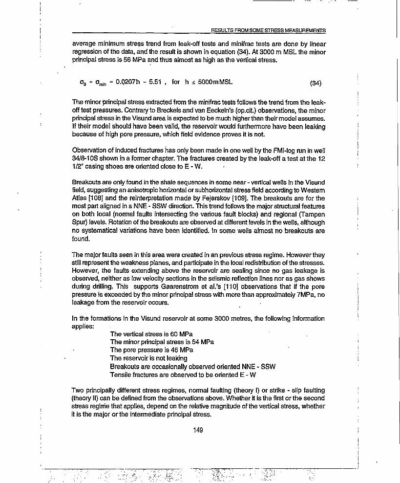
RESULTS FROM SOME STRESS MEASUREMENTS
average minimum stress trend from leak-off tests and minifrac tests are done by linear regression of the data, and the result is shown in equation (34). At 3000 m MSL the minor principal stress is 56 MPa and thus almost as high as the vertical stress.
°3 = °min = 0.0207h - 5.51 , for h i 5000m MSL (34)
The minor principal stress extracted from the minifrac tests follows the trend from the leak- off test pressures. Contrary to Breckels and van Eeckeln’s (op.cit.) observations, the minor principal stress in the Visund area is expected to be much higher than their model assumes. If their model should have been valid, the reservoir would furthermore have been leaking because of high pore pressure, which field evidence proves it is not.
Observation of induced fractures has only been made in one well by the FMI-Iog run in well 34/8-1 OS shown in a former chapter. The fractures created by the leak-off a test at the 12 1/2" casing shoes are oriented close to E - W.
Breakouts are only found in the shale sequences in some near - vertical wells in the Visund field, suggesting an anisotropic horizontal or subhorizontal stress field according to Western Atlas [108] and the reinterpretation made by Fejerskov [109]. The breakouts are for the most part aligned in a NNE - SSW direction. This trend follows the major structural features on both local (normal faults intersecting the various fault blocks) and regional (Tampen Spur) levels. Rotation of the breakouts are observed at different levels in the wells, although no systematical variations have been identified. In some wells almost no breakouts are found.
The major faults seen in this area were created in an previous stress regime. However they still represent the weakness planes, and participate in the local redistribution of the stresses. However, the faults extending above the reservoir are sealing since no gas leakage is observed, neither as low velocity sections in the sdismic reflection lines nor as gas shows during drilling. This supports Gaarenstrom et al.’s [110] observations that if the pore pressure is exceeded by the minor principal stress with more than approximately 7MPa, no leakage from the reservoir occurs.
In the formations in the Visund reservoir at some 3000 metres, the following information applies:
The vertical stress is 60 MPa The minor principal stress is 54 MPa The pore pressure is 46 MPa The reservoir is not leakingBreakouts are occasionally observed oriented NNE - SSW Tensile fractures are observed to be oriented E - W
Two principally different stress regimes, normal faulting (theory I) or strike - slip faulting (theory II) can be defined from the observations above. Whether it is the first or the second stress regime that applies, depend on the relative magnitude of the vertical stress, whether it is the major or the intermediate principal stress.
149

RESULTS FROM SOME STRESS MEASUREMENTS
Theory I:The observed stresses may suggest a normal faulting stress regime if the integrated vertical stress (60 MPa) is the major principal stress. The measured leak-off test- and minifrac values represent the minor principal stress (56 MPa) which is subhorizontal and parallel to the breakouts (NNE - SSW). The intermediate stress is subhorizontal and perpendicular to the breakouts and in the order of the vertical stress.
Theory II:The observed stresses suggest a present strike - slip stress faulting regime if the integrated vertical stress (60 MPa) is the intermediate principal stress. The measured leak-off test- and minifrac values (56 MPa) represent the minor principal stress and is sub-horizontal with a trend parallel to the breakouts. The major principal stress is oriented parallel to the observed sub-vertical fractures (WNW - ESE) with a magnitude higher than the vertical stress to create the breakouts.
Theory I or the normal faulting stress regime is unlikely because it suggests a near isostatic stress field to produce the observed breakouts and aligned fractures recorded by FMI after the leak-off test in well 34/8-1 OS. Theory II or the strike slip faulting regime is the most likely since anisotropic horizontal stresses can be responsible for the aligned tensile fractures and breakouts. Thus, the major principal stress should be horizontal and exceed the measured vertical stress.
Theory II or the strike slip faulting regime is also favoured by Wiprut et al. [111]. They use the data presented above as input information to the suite of computer codes developed by Peska and Zoback [112] called Stress and Failure of Inclined Boreholes to constrain the full stress tensor at 2800 metres depths in the 34/8-1 OS well. They show that the major horizontal stress is the major principal stress at 72 MPa exceeding the vertical stress by 40 percent, and that the other stresses are as proposed in this presentation.
Discussions
To visualize the difficulties and by that the possibilities involved in assessing the minor principal stress measured by hydraulic fracturing and overcoring, several measurements and observations have been conducted and related.
Measurements at Daleelven show that although target depth was not reached, it was still possible to conclude that the proposed design was feasible since the critical minimum water pressure was exceeded above the proposed tunnel. In Fossmark the large scale failure of intact rock support the hydraulic fracturing assessment of the minor principal stress. Without the experienced failure it would have been almost impossible to interpret the correct value for the minor principal stress since a considerable scatter was inherent in the measurements. Comparing overcoring and hydraulic fracturing would even further confuse the issue because the overcoring minor principal stress is low with a large scatter related to it. The overcoring measurements also underestimates the minor principal stress
150

RESULTS FROM SOME STRESS MEASUREMENTS
significantly. The inconclusive stress measuring results must be related to a complicated rock mass with partly open fractures perturbing the stresses. At Vinstra where the measuring conditions are favourable, the overcoring measurements still underestimate the minor principal stress. The minor principal stress can be established with confidence by any of the used hydraulic fracturing procedures since they all give almost identical values. Finding it out whether the absolute value is correct is impossible because it has not been qualified by any natural (large scale) failure by hydraulic fracturing. An inconsistency between the minor principal stress measured by overcoring and hydraulic fracturing exists. However, both measuring results exceed the maximum inner water pressure in the waterways and therefore a safe design is suggested.
Two issues emerge from the discussion above and must be addressed: why do overcoring rock stress measurements underestimate the minimum principal stress that constrains water in unlined waterways, and why is the minor principal stress lower when estimated from overcoring than from hydraulic fracturing stress measurements? The inconsistency in the measuring results must be attributed to the two different bases of the techniques; elastic compliance and fracturing mechanics, besides different volumes of rock involved in each test. Furthermore are hydraulic fracturing measurements more likely to give representative results because they resemble miniature filling situations and thus likely to interpret the failure mechanisms and thus the failure stress most properly.
Reviewing the discussion on measurement of elastic properties and the strain measuring accuracy of the NTH cell from the previous chapters, implies that two factors are the key issues to its unsatisfactory rendition of the minor principal stress. The first factor is the measuring technique that does not capture all the released strains during overcoring. The second factor is the use of improper elastic properties that do not incorporate or adjust properly for strain losses in the coupled system of measuring bridge, electric circuits, strain gauge, adhesive and rock. If these to factors are unresolved, it is likely that the measured overcoring minor principal stress will be too small.
Hanssen and Hansen [113] presented the minor principal rock stress from overcoring measurements and instantaneous shut-in pressure versus maximum static operational water pressure from several hydropower projects to show how the minimum principal stress varied. The overcoring measuring results that were the basis for their discussion have been recalculated according to the recommended code of practice outlined in the previous chapters. Additional measurements have been added to the list, including the results presented in this chapter. All the results are shown in Table 50 and Figure 98. The localities for the last two data sets in the table have been disguised. The rest of the data sets refer to the main hydroelectric power station where the measurements have been done.
In Table 50 and Figure 98 the differences between the minor principal stresses from overcoring and hydraulic fracturing are shown. Stresses obtained by overcoring are at minor 2 MPa lower than the corresponding hydraulic fracturing measurements. The exception to this is seen in measurements from Fossmark and Tafjord K5 where natural hydraulic fracturing and hydraulic jacking have occurred during either commissioning or operation. These to sites plot in an area giving a low factor of safety. Measurements conducted at ACE plot with a similar factor of safety, and should therefore not be completed with unlined
151

RESULTS FROM SOME STRESS MEASUREMENTS
waterways. Measurements conducted atTafjord K1, Osa, Ormsetfoss and Kvilldal show the opposite trend, where the overcoring measurements exceed hydraulic fracturing measurements. Ail these measurements were conducted in fractured rock masses where the pumping capacity in the hydraulic fracturing equipment was too small or the tests were too short for a proper evaluation of the results.
If both overcoring and hydraulic fracturing measurements are used to assess the safe design of an unlined waterway with the present equipment, the hydraulic fracturing minor principal stress should exceed the maximum inner water pressure in the critical waterway. It should furthermore surpass or be equal to the minor principal stress from overcoring stress measurements to form a sound decision for the engineering question.
Table 50 Overcoring rock stresses and their quality rating listed together with hydraulic fracturing measurements in hydroelectric powerplants. Theoretical and measured vertical stresses and maximum inner water pressure are given.
HYDRO POWER HPP Pw QRG a2 o3 PsPLANT
BRATTSET BRA 2.4 4.6 B 4.7 13.1 6.3 0.75 5.1DALEELVEN DAL 2 4.2 - - - - - 3.2FOSSMARK FOS 3.6 7.1 C 7.4 8.3 6.9 2.72 2.7JOSTEDAL JOS 11.5 13 C 19.9 26.5 15 7.9 12.5KOBBELV KOB 6 20.7 B 16.8 22.8 15.3 9.4 -
KVILLDAL KVI 4 7.8 B 9.3 9.93 7.1 5.3 4.6MEL MEL 7.5 9.9 B 18.4 23.1 21.4 5.3 8.0NYSET-STEGGJE NYS 9.7 23.4 C 21.1 22.5 20.1 15.4 15.1ORMSETFOSS ORM 3.8 5.8 B 10.6 13.7 9.3 6.8 4.0OSA OSA 1.9 3.1 C 6.7 12.03 6.2 5.4 2.6SILDVIK SIL 5.4 10.4 B 10.6 22.3 20.8 9.4 -S0RFJORD S0R 4.5 6.0 B 4.1 10.0 5.5 2.4 -
TAFJORD K1 TK1 1.7 1.0 C 6.3 13.0 6.3 4.8 3.7TAFJORD K5 TK5 7.7 13.0 B 7.6 14.4 7.9 5.5 • 8.0TJODAN TJO 8.9 16.9 B 21.6 21.6 6.4 6.1 13.1TORPA TOR 4.4 5.4 C 5.21 6.07 4.5 3.9 4.8VIGDAL .VIG 5.8 10 C 7.0 11.4- 9.8 3.5 6.0VINSTRA VIN 4.4 7.2 B 8.4 13.3 10.4 5.1 7.2ACE ACE 8 10 B 13.4 14.9 10.0 5.7 5.6BDF BDF 1.8 6.6' B 6.8 9.6 7.6 3.9 7.0
HPP Hydro power plant (abbreviations)pw Maximum inner water pressure o« Theoretical vertical stressQRG Quality rating of overcoring stresses .ov Measured vertical stresso, Major principal stress °2 Intermediate principal stresso3 Minor principal stress Ps Minor principal stress from hydraulic
' fracturing
In any applications of stress measurements, evaluating the results and relating them to other information is important. This has been necessary in assessing the overcoring rock stress measurements’ ability to render a probable minor principal stress. In petroleum engineering where no single measuring technique exists to find the full stress tensor, this is even more important. Combination of observations with different bases can give sound assessments of the in-situ stresses. Electrical logs correlated to density measurements give
152

RESULTS FROM SOME STRESS MEASUREMENTS
a continues vertical stress log. Pore pressure measurements and various logs give an estimate of the pore pressure distribution through the formations penetrated by a single well. Leak-off and minifrac tests from neighbouring wells can be combined to establish a minor principal stress envelope. When these logs are combined with geologic knowledge and observations of fractures, borehole breakouts and the drilling history, the full stress tensor and its development with depth can be constrained.
16.00
□ TJO
12.00 —
8.00 — + JOS
DBDF + OKM /
4-TJO
4.00 —t VIG
+ S0R
+ BRA
16.0012.00Inner maximum waterpressure [MPa]
Figure 98 Measured minor principal stresses obtained by overcoring (red cross) and hydraulic fracturing (blue open squares) in critical points in hydroelectric power stations plotted versus the inner maximum water pressure. Lines representing factor of safety from 0,75 through 1,50 are also shown.
153

RESULTS FROM SOME STRESS MEASUREMENTS
Conclusions
From the field tests, the available measurements and observations, this investigation shows that the minor principal stress measured by overcoring is unsuitable to be used as a design guideline for unlined waterways. An unknown factor between the minor principal stress measured by hydraulic fracturing and overcoring insists on this. However, if the measured overcoring minor principal stress significantly exceeds the proposed maximum inner water pressure, its use can be recommended for this purpose.
In fractured rock masses the minor principal stress obtained by hydraulic fracturing may not be conclusive in the assessment of safe design of unlined waterways. This will be dependant of the available pump capacity during testing. This problem can sometimes be evaded by injecting large amounts of water into the rock mass to fill the fractures before a small section of the borehole is tested. The minor principal stress can now be interpreted as the opening and closure pressure during a slow jacking of the existing fractures.
Combination of several data with different bases may successfully be used in constraining the full stress tensor either in a single position as in Fossmark hydropower project, or its development through various formations in long wells as in the Visund oil and gas field.
154

FINAL CONCLUSIONS AND RECOMMENDATIONS FOR FUTURE WORK
FINAL CONCLUSIONS AND RECOMMENDATIONS FOR FUTURE
WORK
Rock stresses are, with the mechanical properties of rock, important to the safe construction and operation of all man made structures in rock, whether in mining, civil or petroleum engineering. The crucial issue is their relative magnitudes and orientation.
The main objectives with the present work have been to develop equipment and methods for further rock stress assessment, reevaluate the existing overcoring rock stress measurements done by NTH / SINTEF and possibly, relate this information to the present geological setting. The work has been carried out both in the field and in the laboratory. Before going out in the field, the equipment for hydraulic fracturing was constructed, and minor improvements were added to the overcoring rock stress measuring field technique. In the field, rock stresses were measured by the overcoring and the hydraulic fracturing technique. An observation technique to assess likely high stresses was developed. In the laboratory, tests were carried out to be able to appraise the present overcoring technique. A new method were developed that incorporates a statistical way of assessing the results from rock stresses measured by overcoring using the NTH cell.
The main topics of this work have been:
1. The present procedures using the NTH cell was investigated. A new statistical method to assess overcoring rock stress measurements using the NTH cell have been developed. The method has been implemented in a usable computer code under contract by an independent consultant. Furthermore, an improved code of practice for overcoring rock stress measurements using the NTH cell have been proposed, including minor changes to the present equipment.
2. The NTH cell has been tested in the laboratory, and its ability to reproduce the applied strains, and thus stresses have been investigated.
3. With basis in these tests and the earlier in-situ measurements, a quality ranking ■ system for overcoring rock stress measurements using the NTH cell were developed and applied to all existing complete measurements.
4. All existing data on overcoring rock stress measurements using the NTH cell were retrieved and reevaluated to extract information on the regional stress distribution.
5. A complete hydraulic fracturing rig was constructed, and a code of practice and evaluation was proposed to collect information on the minor principal stress.
155

FINAL CONCLUSIONS AND RECOMMENDATIONS FOR FUTURE WORK
6. The effect of leak-off tests on the surrounding wellbore has been investigated, and a revised procedure to get information on the minor principal stress was proposed. Additionally, an integrated approach was used to investigate all three principal stresses.
7. Compound rock stress determination was proposed for increased understanding of the state of stress. Field measurements were carried out to investigate if the minor principal stress measured by overcoring was consistent with results from hydraulic fracturing rock stress measurements. Combination of different ressults were also used in the Visund petroleum field.
8. Systematic mapping of the surface exfoliation intensity in the larger Kobbelv area, tunnel mapping and overcoring rock stress measurements were used to investigate the stress regime active in the. field.
Main conclusions
The main conclusions in relation to the above topics are:
1. Evaluation of the current use of the NTH cell.
• The angular accuracy when installing the NTH cell was increased to within 0,1 ° by installing a high precision angular measuring device in the installation tool.
• Stress concentrations caused by poor core drilling was estimated to influence the strains by more than 20 percent, and non-coaxial core drilling will be detrimental to any stress calculation. Proper core drilling was therefore regarded as one critical factor to successful stress determination.
• A method of incorporating all sources of uncertainty related to the measured principal stresses was devised. The uncertainty is described by the standard deviations of the calculated mean principal stresses. The resulting computer program that was programmed by an independent consultant was used in the subsequent evaluation.
2. Laboratory testing of the NTH cell
• In calculation of the stresses, strains from 4 to 5 NTH cells, which functionality has been controlled by the biaxial modulus chamber, should be used. If more strains are included in the calculations, the standard deviation of the mean stresses increases without any positive effect on the mean stress magnitudes. Furthermore, should a streamlining factor of 1 be used to reject any unidentified outlying strains, and the number of calculations should be kept as high as possible.
156

FINAL CONCLUSIONS AND RECOMMENDATIONS FOR FUTURE WORK
• Evaluation of the laboratory tests-on metals and three rock types showed that elastic properties obtained from testing the overcored hollow cylinders containing NTH cells in the biaxial modulus chamber gave the best results. This method should preferably be used both in laboratory and field measurements. Elasticproperties obtained from solid 62 millimetres diameter cores sometimes show Youngs moduli 50 percent lower than those obtained from pressurising hollow cylinders containing NTH cells.
• The relative standard deviation of the calculated major principal stress decreased when the applied stress increased for all tests.
• The measured strains, and thus the calculated stresses increase linearly with increasing applied stress under laboratory conditions.
• The relative standard deviation of the calculated major principal stress, increased to 17 percent at 20 MPa radial loading when granite samples with grain size corresponding to the strain gauge length were tested. It decreased to 5 and 10 percent when fine grained and mono-crystalline rocks were tested. In tests run on metal samples, the standard deviation of the mean principal stress became even lower.
• The calculated mean major principal stresses were consistently close to the applied stresses, irrespectively of sometimes high relative standard deviation of the calculated major principal stresses.
• The calculated principal stress orientations are very robust to strain outliers, and normally within 1 °, but 3° have been observed, of the applied stress direction under laboratory conditions.
3. Reevaluation of existing overcoring rock stress measurements using the newtechnique.
• Rock stresses measured by overcoring using the NTH cell was quality ranked according to the magnitude of the calculated mean major principal stress and its standard deviation.
• Four empirically assigned quality groups were devised, ranging from the highest • quality called Group A, through the lowest Group D. The bulk part of the field
measurements until now classifies as Group B and C, while laboratory tests under controlled conditions classify as Group A and B, depending on grain size and Youngs moduli.
• Of more than 200 measurements in different localities, 155 complete measuring sets were extracted from the archives of NTH / SINTEF and could be recalculated. The results are shown in the text. Five measurements were assigned to quality rank A, 73 to B, 53 to C and 24 to D.
• Unbiased statistical analyses of all stress measurements support the empirically assigned stress quality groups.
157

FINAL CONCLUSIONS AND RECOMMENDATIONS FOR FUTURE WORK
4. Implications to the regional stress field
• High horizontal stresses have been prevailing in the western part of Fennoscandia from reevaluations of overcoring rock stress measurements by the NTH cell.
• Thrust faulting (reverse) stress regimes were observed towards the shallower part of the upper 1000 metres of the crust, succeeded by strike slip faulting regimes and finally normal faulting stress regimes towards the deeper regions.
• Irrespectively of depth or locality, high stresses were measured all over the western Fennoscandia. However, normal faulting stress regimes were predominantly found in the western part intermingled with the two other stress regimes. To the east, subsequently strike slip and thrust faulting stress regimes are found respectively.
• The measured high horizontal stresses, however, relative shallow compared with normal seismic activity, were found to support seismotectonic observations and measurements.
• Whether the stress regime was normal or thrust faulting, the measured stresses exceeded the basic failure criterions for frictional sliding on preexisting fractures. Although the failure criterions perhaps were underestimated, the rock stress measurements still suggested that the upper part of the crust was in a continuous state of failure.
5. Equipment for hydraulic fracturing
• A fully equipped modular rig for hydraulic fracturing including packers was built and field tested. It was built with the following characteristics:
Power pack:Water pump capacity:Flow metre capacity:Pressure transducers:Computer logging:Measuring depth:Packer size:Winches pull force:
30 kW diesel-hydraulic engine35 l/min at 40 MPa0.1 l/min - 40 l/min (±0.04 l/min)0-50 MPa (±0.01 MPa)1 Hz (all channels)280 mRange of a diameter from 48 mm to 150 mm 25 kN
• Based on practical experience after several assignments, a code of practice to assess the principal stresses was formulated.
6. Leak-off tests
* Leak-off tests was the only data readily available to estimate the minor principalstress in petroleum wells, and it is widely used. However, if care was not exercised, ambiguous interpretations would result. In one study, only 25 percent of the collected material was useable for stress determination.
158

FINAL CONCLUSIONS AND RECOMMENDATIONS FOR FUTURE WORK
• Leak-off tests were shown to be just as harmful to wellbore stability as ordinary drilling operations, i.e. there was no reason that these tests should be left unheeded, or not properly executed.
• At present, standard methods of doing leak-off tests are nonexisting. The information available from the extended leak-off tests justified a proposed code of practice, with a quality ranking scheme based on the method'pressures was recorded.
7. Compound rock stress determination
• Compound rock stress determinations were found successful, and should be encouraged whenever possible.
• The in-situ measurements suggested that care should be exercised if the minor principal stress measured by overcoring were used for the design of unlined high pressure water ways.
• The minor principal stress was measured by overcoring and hydraulic fracturing rock stress measurements. Discrepancy, often more than 2 MPa, was found between the two measuring methods. Systematically, overcoring underestimated the minor principal stress compared with hydraulic fracturing. In only one instance it proved possible to estimate the in-situ minor principal stress. In the Fossmark hydro power pressure shaft, the rock mass failed during filling. Measurements by hydraulic fracturing were ambiguous, while overcoring rock stress measurement underestimated the minor principal rock stress by more than 2 MPa. The composite measurements and field observations suggested that the design would have failed, however, in retrospect.
• Several measurements and observation methods were used to constrain the stresses in the offshore Visund petroleum field. The likely orientations of the stresses are horizontal WNW, vertical and horizontal NNE for the major, intermediate and minor principal stresses. At some 3000 metres below the sea level the major principal stress exceeds the vertical stress that in turn slightly exceeds the minor principal stress. These observations pointed to Visund being influenced by higher horizontal stresses than what is usual in the North Sea.
8. Morphological rock stress indicators and the regional stress field
• In the larger Kobbelv area, the presence and orientation of regional high horizontal stress were shown by surface mapping of the intensity of exfoliation spalling. The method was proposed as one way of assessing possible high stresses.
• Overcoring rock stress measurements showed large horizontal stresses consistent with the surface related findings. Due to the consistency in the measurements, it was suggested that the measured stresses show the regional system. This was supported by correlation to seismic observations.
• Mapping of spalling in the hydropower tunnels in the area also supported the assumption that high horizontal stresses are prevalent in the area.
159

FINAL CONCLUSIONS AND RECOMMENDATIONS FOR FUTURE WORK
• In the upper 1000 metres of the Earth’s crust in the larger Kobbelv area, the easterly and northerly principal stresses are approximately 23 MPa and 15 MPa.
RECOMMENDATIONS FOR IMPROVEMENT OF ROCK STRESS ASSESSMENTS
• Revised code of practice for overcoring rock stress measurements using the NTH cell
1. Drilling of the measurement hole into the rock mass to the point where the stresses are to be measured. Drilling bit size is 76 mm diameter, giving cores with 62 mm diameter.
2. Flattening the end of the hole with a facing drill bit.3. Drilling of a concentric borehole approximate 25 cm further into the rock mass, with bit size
of 36 mm diameter, giving cores with 22 mm diameter.4. Inspection of 22 mm cores to find the placement of the measuring cell, ensuring no
fractures or lithology change nearby.5. Flushing and drying of the measuring area in the hole.6. Installation of the measuring cell, including orienting and cementing.7. Taking initial readings of strain gauges.8. Overcoring of measuring cell and drilling totally 50 cm, which also gives undisturbed rock
core fortesting purposes.9. Measuring of post-overcoring strains for each strain gauge.10. Calculation of strain relief values by subtracting initial from post-overcoring strain values.11. Measuring the borehole orientation.12. Determination of elastic moduli and functionality of the overcored measuring cell by use of
the biaxial modulus chamber.13. Calculation of principal stresses and their orientation for each overcored measuring cell.14. Evaluation of results and decision whether to do more measurements.15. Laboratory determination of mechanical and elastic properties on 62 mm cores.16. Evaluation of results with respect to the engineering question to be solved.
• Proposed code of practice for hydraulic fracturing
1 Start the data logging computer, and establish zero level for all gauges.2 Do frictional pressure loss calibrations.3 Increase packer pressure until just below anticipated shut-in pressure.4 Increase injection pressure to one third of packer pressure.5 Monitor pressure gauges for any pressure drop indicating leakages.6 Decrease injection pressure to zero.7 Increase injection pressure at a rate such that fracturing 1 jacking is accomplished in 5-10
minutes (higher pressure, takes longer time).8 Keep the water flowing into the test section as short time as possible, but until a constant
'flow rate has been established.9 Close the shut off valve and monitor the injection pressure decay.10 Open bleed off valve and let the section bleed off.11 Repeat step 7 to 10 once.12 Activate the check valve in injection flow line.13 Repeat step seven to eight.14 Decrease injection pressure at the same rate as it was increased.15 Monitor pressure decay after the check valve has closed.16 Repeat step 13 to 15 once.
160

FINAL CONCLUSIONS AND RECOMMENDATIONS FOR FUTURE WORK
17 Bleed off injection pressure and deflate the straddle packer, pull out of hole.18 Make an oriented imprint of the test section.19 Before equipment isremoved from the location a quality check of the registered data is
conducted to ensure good measurements. If bad results are found, more testing is needed.
• Proposed code of practice for leak-off tests
1 Use the mud loggers bottom hole assembly pressure gauges with logging rates of 1 Hz, measuring both annulus and drill string pressures with backup equipment on the topside pump. A bottomhole pressure transducer is vital to the integrity of the test.
2 Circulate out mud from the annulus until entering and returning mud has equal densities measured topside.
3 Close the well at the annulus and increase the well pressure by pumping at a constant rate through the drillpipe. Use dedicated pumps or the rig cement pumps with a flow rate of approximately 50 l/min (This rate can be .discussed).
4 Continue pumping with a constant rate until the pressure drops or five (ten) minutes after pressure has stabilized.
5 Shut-in the well and register the'pressure decline until the pressure has stabilized, or limited to minimum five minutes and maximum ten minutes.
6 Open the well and flow back at the same rate for five (ten / twenty) minutes while recording the returned volume and the possible pressure decline.
7 Immediately repeat steps 3 to 5.8 If the two shut-in decline pressures differ more than 5 bar, repeat steps 2 to 5.9 Plot time charts of pressure and flow.10 Plot pressure versus cumulative injected volume.11 Plot pressure versus returned volume.12 Evaluate leak-off pressure, formation fracture pressure and fracture closure pressure
• Proposed quality rating of tests used to assess the minor principal stresses based on the level of completeness and pressure registration.
Topside, Manual recording Topside, digital recording Downhole, digital recording
FIT LOT ELOT Minifrac
F "E E CE E D CD C B A
161

FINAL CONCLUSIONS AND RECOMMENDATIONS FOR FUTURE WORK
• Proposed code of practice for morphological mapping of surface spalling
1 All exfoliation areas considered must extend at minor one kilometre in any direction2 Qualifying description for observations in mountain sides.
a No visible exfoliationb Relative middle intensity exfoliationc Relative intense exfoliation
3 Presentation of data in rose diagrams for each qualifier and for the total data set
Recommendations for further work
The research work presented in this thesis has led to additional ideas that could be further investigated. The following ideas pertinent to this research work are recommended for further investigation regarding rock stress measurements and rock stress evaluation:
NTH cell• The calculated mean principal stresses are calculated with high accuracy under
laboratory conditions. They still have a relative high associated standard deviation. The possible reasons behind these high standard deviations should be further investigated.
• Explore the possibility to use 4-gage composite strain gauges to increase the redundancy in the strain measurements.
• Use six-wire full bridge circuits to complete the active strain gauges in the NTH cells.
• Isolate the electrical contact of the NTH cell completely from environmental influence during overcoring.
• Construct a reusable memory module integral to the NTH cell to monitor strains, temperature and core bit advance during overcoring, and possible postovercoring strain relaxation. Dump the data to the computer where the stresses are calculated.and use a visualization software to acquire the actual strains for each strain gauge.
• If the biaxial modulus test chamber is used to assess the constitutive properties of overcored “new”.NTH cells comprising 12 strain gauges, finding which constitutive model is most appropriate for the stress calculation is possible.
• If other constitutive models are envisioned, they can be readily integrated in the existing computer code for further evaluation.
162

FINAL CONCLUSIONS AND RECOMMENDATIONS FOR FUTURE WORK
Leak-off tests• Implement standards for leak-off or extended leak-off tests.• Create an atlas of type curves for leak-off tests to simplify the evaluation of test
results.• Continue to systematizegood quality leak-off data to seek regional trends and
relate them to vertical stresses and pore pressures.
Hydraulic fracturing• Reduce the number of cables and hoses needed in the hole by redesigning the
top head of the packer.• Install pressure transducers in the packer-assebly.• In the hydraulic fracturing equipment a flow metre should be installed in the
return line to observe the bleed-back rate and volume.• Continue the evaluation of hydraulic fracturing measurements, especially should
test procedure and test results evaluated be standardized.
Stress evaluations• Composite stress evaluations should be encouraged to pursue the complete
stress tensor under various conditions• A systematic investigation into how stresses change according to lithological
variations, and specially how stresses vary in layered strata with changing constitutive behaviour.
164

LIST OF ABBREVIATIONS
ASTMCSIRCSIRODnVAISRMHBMLuHNGINPDNTHNVESINTEFSPESSPBStatoilUSBMVISTAASRCBILDSCAELOTFITFMIFMSFRSDBHTPFLOTMSLRKBTVD
abEgh
PoPcp,PmP=PpPrPsPoPwq„SD,T
American Society for Testing and Materials South African Council for Scientific and Industrial Research
Commonwealth Scientific and Industrial Research Organization, Australia The Royal Norwegian Academy of ScienceInternational Society for Rock MechanicsHottinger Baldwin MesstechnikUniversity of LuleaNorwegian Geotechnical InstituteNorwegian Petroleum DirectorateNorwegian Institute of Technology, University of TrondheimNorwegian State Power BoardThe Foundation for Scientific and Industrial Research at the Norwegian Institute of TechnologySociety of Petroleum EngineersSwedish State Power BoardThe Norwegian State Oil Company asUnited States Bureau of MinesJoint research venture between DnVA and StatoilAnelastic strain recoveryDigital Circumfericial Borehole Image Log, product of Western Atlas International Differential Strain Curve Analysis Extended Leak-off Test Formation Integrity TestFormation Micro Imager, product of Schlumberger Formation Micro Scanner, product of Schlumberger Fennoscandian Rock Stress Data Base Hydraulic Testing of Preexisting Fractures Leak-off TestDepth referred to Mean Sea Level Depth referred to Rotary Kelly Bushing True vertical Depth
Inner radius [mm]Outer radius [mm]Young's Modulus [GPa]Gravitational acceleration [m/s2]Vertical overburden [m]IndexInitial pore pressure [MPa]Fracture closure pressure [MPa]Fracture initiation pressure [MPa]Measured pore pressure [MPa]Fracture opening pressure [MPa]Fracture propagation pressure [MPa]Fracture reopening pressure [MPa]Instantaneous shut-in pressure [MPa]Outer pressure [MPa]Water pressure [MPa]Water flow [l/min]Standard deviation for q [MPa]Formation fracture strength [Mpa]
165

a Biot factor|3 Failure angle [°]n. Relative standard deviation of the ijth mean principal stress [%]e Strain [pS]e‘ Strain under consideration [pS]ea Axial strain [pS]Gy Theoretical calculated axial strain [pS]ee Tangential strain [pS]ea Theoretical calculated tangential strain [pS]©i Plunge of ith principal stress [°]v Poisson's Ratiop Specific weight [kg/dm3]o'mac Maximal effective tangential stress [MPa]o'nm Minimal effective tangential stress [MPa]aa Axial stress [MPa]oc Uniaxial compressive strength [MPa]Otmax Measured maximal horizontal stress [MPa]Otoin Measured minimal horizontal stress [MPa]C,* Effective gravitational vertical stress [MPa]ow Gravitational vertical stress [MPa]
o, Far-field stress at infinity [MPa]a, ith principal stress [MPa]o, Tensile strength [MPa]ov Measured vertical stress [MPa]o'* Effective gravitational horizontal stress [MPa]o* Gravitational horizontal stress [MPa]og Tangential stress [MPa]<!>, Trend of ith principal stress [°]^hnax Trend of measured maximal horizontal stress [°]<p Angle between active axis and the direction under consideration [°]rj> Angle of rotation in the plane perpendicular to the borehole axis [°]
166

REFERENCES
1. Li, B. (1967). BERGMEKANIKK, En undersekelse av spenningsforholdene i rom- og pilarfeltet ved Kjerholt kalkstensgruve og av kalksteinens mekaniske egenskaper, Bergverkenes
• Landssammenslutnings Industrigruppe Teknisk Rapport nr.6,106 p.
2. Sigmond, E.M.O. (1992), Bedrock map of Norway and adjacent ocean areas. Scale 1:3 mill. Geological Survey of Norway
3. Fossen, H., K.G.Ho!ter, J.Hesthammer, G.Mangerud, O.Martinsen and R.H.Gabrielsen (1995), Jurassic Park - neermere enn vi tror, Problemeri Bjoraytunnelen. Geonytt 3-95, pp. 3-6, Trondheim
4. Fasrseth, R.B., Gabrielsen, R.H. and Hunch, C.A. (1995), The influence of basement in structuring of the North Sea Basin offshore Southwest Norway. Norsk Geol. Tidsskrift, Vol. 75, pp. 105-119, Oslo
5. Ziegler, P.A. (1990), Geological atlas of Western and Central Europe 1990. Shell Internationale Petroleum Maatschappij B.V. 239 pp.
6. Muir Wood, R. (1989), Extraordinary deglaciation reverse faulting in northern Fennoscandia. In.: Gregersen, S. and Basham, P.W.(eds.), Earthquakes at North-Atlantic passive margins: Neotechtonics'and postglacial rebound. NATO ASI Series, Series C: Mathematical and physical sciences - vol. 266, Kluver Academic Publishers pp.141-173.
7. Olesen, O., S.Gjelle, H.Henkel, T.A.Karisen, LOIsen and T.Skogset (1995), Neotectonics in the Ranafjorden area, Northern Norway. Nor. Geol. Unders. Bull 427.
8. Brekke, H., Kalheim, J.E., Riis, F., Egeland, B., Blystad, P., Johnsen, S. and Ragnhildstveit, J.(1992), Two-way time map of the unconformity at the base of the Upper Jurassic (north of 69N) and the unconformity at the base of the Cretaceous (south of 69N), offshore Norway, including the main geological trends onshore. Scale 1:2 mill. NPD Continental Shelf Map No. 1. The Norwegian Petroleum Directorate/The Geological Survey of Norway.
9. Han, D. and Wahr, J. (1989). Post-glacial rebound analysis fora rotating earth. In: Cohen, S.C. and Vanicek, P. (Eds.) Geophysical Monograph 49, IUGG Volume 4 Slow deformation and transmission of stress in theEarth. pp.1 - 6.
10. Anda, E. (1986). Nordvestlandet: Regional topograti og den tertiaere landheving. ImGeolognytt nr.21 Proc. Norsk Geologisk Forenings X. Landsmote Trondheim 16.-18. januar 1986,
11. Ahjos, T. and Uski, M. (1992). Earthquakes in northern Europe in 1375 - 1989. Tectonophysics, 207(1992), pp.1 -23.
12. Olesen, O., Henkel, H„ Lite, O.B., Mauring, E., Panning, J.S. and Torsvik, T.H. (1992)Neotectonics in the Precambrian of Finnmark, northern Nomay. Norsk Geologisk Tidsskrift, Vol.72, pp. 301-306.
13. Anundsen, K. (1989), Late Weichselian relative sea levels in southwest Norway: observed strandline tilts and neotectonic activity. Geologiska Foreningen i Stockholms Forhandlingar 111, 288-292.
14. Bungum H., Alsaker A., Kvamme LB. and Hansen R.A. (1991), Seismicity and seismotectonics of Nomay and nearby continental shelf areas. J. Geophys. Res'. 96:2249-2265.
15. Ramberg, I.B., Gabrielsen, R.H., Larsen, B.T. and Solli, A. (1977), Analysis of fracture pattern in Southern Nomay. Geol. Mijnbouw., 56:213 - 310.
16. Gabrielsen, R.H. and Ramberg, LB. (1979), Fracture pattern in Nomay from Landsat imagery: results and potential use. Proc. Norw. Sea Symp. Tromsa, NSS/23:1 - 28.
167 .

17. Aanstad, K.M., Gabrielsen R.H., Hagevang, T., Ramberg, I.B. and Torvanger, O. (1981). Correlation of off-shore and on-shore structural features between 62 N and 68 N, Norway. Proc. Norw. Symp. on Exploration, Bergen, Norw. Pet. Soc., NSE/11:1-24
18. Gabrielsen, R.H., Ramberg, I.B., Mark, M.B.E. and Tveiten, B. (1981), Regional gelogical, tectonic and geophysical features of Nordiand, Norway. Earth Evol. Sci., 1:14-26.
19. Rathore, J.S. and Hospers, J. (1986), A lineaments study of southern Nomay and adjacent offshore areas. Tectonophysics, 131:257-285.
20. Lippard, S.J. and Roberts, D. (1987), Fault systems in the Caledonian Finnmark and the southern Barents Sea. Norges geologiske undersekelse, Bull.410:55-64.
21. Gabrielsen R.H. and Faerseth, R.B. (1989), The inner shelf of North Cape, Nomay and its implications for the Barents Shelf - Finnmark Caledonide boundary. A comment. Norsk Geologisk Tidskrift, Vol. 69, pp. 57-62. Oslo.
22. Stewart, I.J., Rattey, R.P. and Vann, I.R. (1992). Structural style and the habitat of hydrocarbons in the North Sea. In: Larsen, R.M., Brekke, H., Larsen, B.T. and Talleraas, E. (eds). NPT Special Publication 1, Elsevier, Amsterdam, pp.197 - 220.
23. Schmidt, W.J. (1992). Structure of the Mid-Nomay Heidrun Field and its regional implications. In: Larsen, R.M., Brekke, H., Larsen, B.T. and Talleraas, E. (eds). NPT Special Publication 1, Elsevier, Amsterdam, pp. 381 - 395
24. Dengo, C.A. and Rossland, K.G. (1992) Extensional tectonic history of the western Barents Sea.In: Larsen, R.M., Brekke, H., Larsen, B.T. and Talleraas, E. (eds). NPT Special Publication 1,
Elsevier, Amsterdam, pp. 91 -107.
25. Gabrielsen, R.H., Fserseth, R.B., Jensen, L.N., Kalheim, J.E. and Riis F. (1990), Structural elements of the Norwegian continental shelf Part I: The Barents Sea Region. NPD-Bulletin no 6.
26. Shannon, P.M. and Naylor, D. (1989). Petroleum basin studies. Graham and Trotman Ltd, London.p.12.
27. Richardson, R.M., (1992) Ridge forces, absolute plate motions, and the intraplate stress field. J. of Geophys. Res., Vol. 97, No. B8, pp 11739-11748.
28. Stephansson, O. (1988), Ridge push and glacial rebound as rock stress generators in Fennoscandia. Bull. Geol. Inst Univ. Uppsala, N.S. Vol. 14, pp. 39 - 48.
29. Crouch, S.L. (1976), Analysis of stresses and displacements around underground excavations: an application of the displacement discontinuity method. Geomechanics report to the National Science Foundation. Minneapolis: University of Minnesota.
30. Dart, R.L. and Swolfs, H.S. (1992). Subparallel faults and horizontal-stress orientations: an evaluation ofin-situ stresses inferred from elliptical wellbore enlargements. In: Larsen, R.M., Brekke, H., Larsen, B.T. and Talleraas, E. (eds). NPT Special Publication 1, Elsevier, Amsterdam, pp.519-529.
31. Aleksandrowski, P., Inderhaug, O.H. and Knapstad, B. (1992), Tectonic structures and wellbore breakout orientation, in Tillerson, J.R. and Wawersik, W.R. (Eds.) Proc. 33rd U.S. Symp. on Rock Mechanics, pp. 29-37.
32. Harris, R.A. and Simpson, R.W.(1992). Changes in static stress an southern California faults after 1992 Landers earthquake. Nature, Vol. 360,19. November 1992, pp 251 - 254.
33. Stein, R.S., King, G.C.P. and Lin, J. (1992) Change in failure stress on the southern San Andreas Fault System caused by the 1992 magnitude = 7.4 Landers earthquake. Science, Vol. 258. 20.November 1992, pp.1328 -1332.
168

34. Zoback, M.L., Zoback, M.D., Adams J., Assumpcao M., Bell S., Bergman EA„ Bumling P., Brereton N.R., Denham D., Ding J., Fuchs K., Gay N., Gregersen S., Gupta H.K., Gvishiani A., Jacob K., Klein R., Knoll P., Magee M., Mercier J.L, Muller B.C., Paquin C„ Rajendran K., Stephansson O., Suarez G., Suter M., Udias A., Xu Z.H. and Zhizhin, M. (1989), Global pattern of tectonic stress. Nature, 341:291-298.
35. Zoback, M.L. (1992), First- and second-order patterns of stress in the lithosphere: The World Stress Map Project. J. Geoph. Res. Vol. 97, No. B8. pp 11703 -11728.
36. Muller, B., Zoback M.L, Fuchs K., Masdin L, Gregersen S., Pavoni N., Stephanson O. and Ljunggren, C. (1991), Regional patterns of tectonic stress in Europe. J. Geoph. Res. Vol. 97, No. B8.pp 11783-11803.
37. Stephansson, O., Dahlstram, L-O., Bergstrom, K., Myrvang, A., Fjeld, O.K., Hanssen, T.H.,Sarkka, P„ and Vaatainen, A. (1987), Fennoscandian Rock Stress Data Base - FRSDB. Research Report Tulea 1987:06
38. Stephansson, O., Sarkka, P. and Myrvang, A. (1986), State of stress in Fennoscandia. In. Stephansson, O. (Ed.) Proceedings of the International Symposium on Rock Stress Measurements, Stockholm, pp. 21 - 32. Lulea: CENTEC Publishers.
39. Bell, J. Sebastian (1993), The global sedimentary basin stress project of the International Lithosphere Program. Poster P-71,55th Meeting of European Association of Exploration Geophysicists, Stavanger, Norway, June 7-11,1993.
40. Spann, H., Brudy, M. and Fuchs, K. (1990) Stress evaluations in offshore regions of Norway. Terra Nova 3, pp. 148-152
41. Cowgill, S.M., Meredith, P.G., Murrel, S.A.F. and Brereton, N.R. (1992) In situ stress orientations in the Witch Ground Graben, North Sea, revealed by borehole breakouts: preliminary results. In: Hurst, A., Griffits.C.M. and Worthington, P.F. (eds.) Geological Applications of wireline logs II. Geological Society Special Publication No65, pp. 179 -184.
42. Fejerskov, M. (1996) Determination ofin-situ rock stresses related to petroleum activities on the Norwegian Continental Shelf. Dr.lng. Thesis, Norwegian University of Science and Technology, 162 P-
43. Golke, M. (1996), Patterns of stress in sedimentary basins and the dynamics of pull-apart basin formation. Ph.D. Thesis, Vrije Universiteit, Amsterdam, 167 p.
44. Owens, K.A., Andersen, S.A. and Economides, M.J. (1992) Fracturing pressures for horizontal wells. Paper SPE 24822. pp 581 - 588.
45. Teufel, L.W. and Farrell, H.E. (1990). Distribution ofin-situ stress and natural fractures in the Ekofisk field, North Sea. In: Proc. Third North Sea Chalk Symp., Copenhagen, Denmark.
46. Biot, M. A.. (1941), General theory of of three-dimentional consollidation. Journal of Applied Physics, 12, pp.55 - 64
47. Biot, M. A. and Willis, D.G. (1956) The elastic coefficients of the theory of consollidation. Journal of applied mechanics, 78, pp.91-96.
48. Mann, D.M. & Mackenzie, A.S. (1990) Prediction of pore fluid pressures in sedimentary basins. Marine and Petroleum Geology, V.7, pp.55 - 65.
49. Waples, D.W. (1991) Generation and migration of petroleum from abnormally pressured fluid compartments. Bull. AAPG. Vol. 75, pp. 326 - 327.
50. Stainforth, J.G. (1984) Gippsland hydrocarbons - a perspective from the basin edge. APEA Journal, Vol. 24 (1), pp. 91 - 99.
169

51. Barker, C. (1990) Calculated volume and pressure changes during the thermal cracking of oil to gas in reservoirs. Bull. AAPG Vol. 24, pp. 1254 -1261.
52. " Spencer, C.W. (1987) Hydrocarbon generation as a mechanism for overpressuring in the RockyMountain region. Bull. AAPG. Vol. 71, pp. 368 - 388.
53. Caillet, G., Sejoume, C., Grauls, D. & Amaud, J. (1991) Hydrodynamics of the Snorre field area, offshore Norway. Terra Nova, Vol. 3, pp. 180-194.
54. Amadei, B. and Savage, W.Z. (1985). Gravitational stresses in regularly jointed rock masses - A keynote lecture, in: Stephansson, O. (Ed.) Proc. Int. Symp. Fundamentals of Rock Joints. CENTEK Publishers, Lulea, pp. 463 - 473.
55. Savage, W.Z., Amadei, B.P. and Swolffs, H.S. (1986). Influence of rock fabric on gravityinduced stresses, in: Stephansson, O. (ed.) Proc. of the Int. Symp on Rock Stress and Rock Stress Measurements. CENTEK Publishers, Lulei, pp.99 -110.
56. Laitaj, E.Z. & Bielus, LP. (1986) Stress corrosion cracking of Lac du Bonnet Granite in tension and compression. Rock Mechanics and Rock Engineering 19, pp. 71 - 87.
57. Hanssen, T.H., Stjem, G. and Sorlakk, T. (1991) Bergarters mekaniske egemskaper. SINTEF report no.: STF36 A91090, Trondheim.
58. McGill, R., Tukey, J.W., and Larsen, W.A. (1978). Variation of box plots. The American Statistical 32,12-16.
59. Leeman, E.R. (1966), The determination of the complete state of stress in rock from measurements in a single borehole. Council of Scientific and Industrial Research, Pretoria.
60. Kim, K. and Franklin, J. A. (Eds.) (1987). International Society for Rock Mechanics, Commission on suggested methods for rock stress determination. Int. J. Rock Mech. Min. Sci. & Geomech. Abstr. Vol. 24, No. 1, pp.53-73.
61. Myrvang, A. (1970), En bergmekanisk undersokelse ved A/S Rodsand Gruber. Lic.tech. Thesis, University of Trondheim, Norwegian Institute of Technology.
62. Hoffmann, K. (1989), An Introduction to Measurements using Strain Gages, Hottinger Baldwin Messtechnik GmbH, Darmstadt, 291 pp.
63. Amadei, B. and O.Stephansson (1997). Rock Stress and Its Measurement. Chapman & Hall, London, 490 p.
64. Amadei, B. (1983), Rock anisotropy and the theory of stress measurements, Lecture notes in engineering, Vol.2, Springer, New York, 478 pp.
65. Timoshenko,S.P. & Goodier.J.N. (1982), Theory of Elasticity, McGraw-Hill International Book Company, pp. 68-71.
66. Fitzpatric, J. (1962), Biaxial device for determining-tile modulus of elasticity of stress-relief cores. BuMines Rept of lnv.6128. pp.13.
67. Okubo, S. and Fukui, K. (1996), Complete stress - strain curves for various rock types in uniaxial tension. Int. J. Rock Mech. Min. Sci. & Geomech. Abstr. Vol. 33, No. 6, pp.549-572.
68. Lejon, B. (1978). Residualspenningar hos nigra svenska bergarter. M.Sc. thesis, University of Lulea, 68 p.
69. Hiltscher, R., Marina, J. and Strindell, L. (1979). The measurement of triaxial rock stress in deep boreholes and the use of rock stress measurements in the design and construction of rock openings. Proc. 4th Int. Congr. Rock Mech., Montreux, vol. 2, pp. 227 - 234.
170

70. Buen, B. (1977). Residual stresses in rock. Report no. 3, Dept of Geology, Norwegian institute of technology.
71. Myrvang, A. (1974), Note on residual strain measurements in block from Morre hydropower plant, Afjord Norway, unpubl.
72. Leijon, B. (1988), Rock stress measurements using the LuT-gauge overcoring method. Doctoral • Thesis, Lulea University of Technology.
73. Walker J.R., Martin C.D. and Dzik E.J. (1990), Confidence intervals for in situ stress measurements. Int. J. Rock Mech. Min. Sci. & Geomech. Abstr. Vol. 27, No. 2, pp. 139-141.
74. Jupe, A.J. (1994), Confidence intervals for in situ stress measurements. Int. J. Rock Mech. Min.Sci. & Geomech. Abstr. Vol. 31, No. 6, pp. 743 - 747.
75. Effron, B. (1982), The Jacknife, the Bootstrap and other resampling plans. SIAM, Philadelfia, PA.
76. Snider, G. R., Lang, P. A. and Thomson, P. M. (1989), Procedures used for overcore testing during sinking of the URL shaft. AECL Technical Record, TR-389, Chalk River, Ontario, 32 pp.
77. Lu M. (1991), DISC - A computer program for calculation of in situ stress from strains measured in a borehole by overcoring. SINTEF report no.: STF36 F91055.
78. Lu, M. (1993) DISO ver. 2.1 A computer program for calculation of in situ stress from strains measured in a borehole by overcoring, unpubl.
79. Worotnicki, G. (1993) CSIRO Triaxiai Stress Measurement Cell, in: Hudson, J.A. Comprehensive Rock Engineering Vol 3., Pergamon Press, Oxford, pp. 329 - 394.
80. Ruistuen, H. (1993) Collection of output files to evaluate the ability of the computer code DISO to calculate rock stress orientations, unpubl.
81. Garfield, F.M. (1984) Quality assurence principles for analytical laboratories Association of Official Analytical Chemists, Inc., Arlington, pp. 184-191.
82. Zoback, M.L (1992). First-and second-order patterns of stress in the lithosphere: The World Stress Map. J. Geophys. Res. Vol. 97, No. B8, pp. 11703 -11728
83. Fejerskov, M., C.D. Lindholm, H. Bungum, A. Myrvang, R.K. Bratli and B.T. Larsen (1995), Crustal stress in Norway and adjacent offshore regions. Final Report for the IBS-DNM project, Topic 1.3 “Regional Stress Field” 12pp. + 3 app. Unpublished
84. SYSTAT Inc. (1992), SYSTAT for Windows: Statistics, Version 5. Evanston, II, p.81 -105
85. Engelder, T. (1993), Stress regimes in the lithosphere. Princeton University Press, Princeton, New Jersey, p.349 - 360
86. Byeriee, J.D.(1978), Friction in rocks. Pure and Applied Geophysics, vol. 116, p.615 - 626
87. Fairhurst, C. (1965). Measurement of in situ rock stresses with particular reference to hydraulic fracturing. Felsmechanik und Ingenieurgeologi, Vol.2, No.3-4, pp. 129 -147.
88. Kim, K. and Franklin, J.A. (eds.) (1987), International Society for Rock Mechanics, Commission on Testing Methods, method 2: Suggested methods for rock stresss determination using the hydraulic fracturing technique. Int. J. Rock Mech. Min. Sci. & Geomech. Abstr. Vol. 24, No. 1, pp. 53 - 73
89. Enever, J.R., Comet, J.C. & Roegiers, J.C. (eds.) (1992) International Society for Rock Mechanics, Commission on interpretation of hydraulic fracture records. Int. J. Rock Mech. Min. Sci. &Geomech. Abstr. Vol 29, No. 1, pp. 69 - 72
90. Hubbert, M.K. and Willis, D.G. (1957). Mechanics of hydraulic fracturing. Trans. Am. Inst. Min.Eng., 210, pp. 153 - 168.
171

91. Comet, F.H. (1986), Stress determination from hydraulic tests on existing fractures - the HTPF method. In: Stephansson.O. (ed.) Proc. Int. Symp. on Rock Stress Measurements, CENTEK Publishers, pp. 301 - 312.
92. Baumgartner, J. (1987), Anwendung des Hydraulic-Fracturing-Verfahrens fur Spannungsmessungen im geklufteten Gebirge, daigestellt anhand von Messergebnissen aus Tiefbohrungen in der Bundesrepublik Deutschland, Frankreich undZypem. Berichte des Insfituts fur Geophysik der Ruhr-Universitat Bochum, Reihe A, Nr.21,223 p.
93. Rummel, F. (1987). Fracture mechanics approach to hydraulic fracturing stress measurements. In Atkinson, B.K. (ed.) Fracture mechanics of rock, Academic Press Inc (London) Ltd. pp.217 - 239.
94. Detoumay, E., Cheng, A.H.-D., Roegiers, J.-C. and Mclennan,J.D. (1989), Poroelastic consideration in in situ stress determination by hydraulic fracturing. Int. J. Rock Mech. Min. Sci. & Geomech. Abstr. Vol. 26, No. 6, pp. 507 - 513
95. Breckels, I.M. and van Eeckelen, H.A.M. (1982), Relationship between horizontal stress and depth in sedimentary basins. Journal of Petroleum Technology, September 1982, pp. 2191 - 2199.
96. Aadnay, B.S. (1990), Inversion technique to determine the insitu stress field from fracturing data. J.PetSci Eng., Vol.4, pp.127 -141.
97. Caillet, G., Deboaisne, R., Mathis, B. and Roux, C. (1994), The present-day stress regime in some deep structures of quadrant 25, offshore Norway. Bull. Centres Rech. Explor. -Prod. Elf Aquitaine, 18,2, pp. 381 - 390
98. Lone, G. (1995), In Situ Measurements and Rock Mechanics Testing of Overburden Rock from the Ekofisk Field, North Sea. MSc thesis, New Mexico Institute of Mining and Technology, 65 p. Unpublished.
99. Amundsen, O, (1995), Determination ofin-situ stresses from leak-off and extended leak-off tests in the Oseberg field, North Sea. Msc thesis, New Mexico Institute of Mining and Technology, Unpublished.
100. Knapstad, B. (1990), Norsk Hydro Memo on Procedure for Extended Leak Off Test. Unpublished.
101. Kunze, K..R. and Steiger, R.P. (1992), Accurate in-situ stress measurements during drilling operations. SPE Paper 24593, Proc. Of 67th Annual SPE Technical Conference and Exhibition, Washington, pp. 491 -199.
102. Hanssen, T.H. and Myrvang, A. (1986) Rock stresses and rock stress effects in the Kobbelv area, northern Nonway. in: Stephansson (ed.) Proc. of the int. symp. on Rock Stress Measurements, Stockholm.
103. Pegg, E. (1989), Kobbskartunnelen - Store bergspenningsproblemer. Proceedings of Praktisk bergmekanikk fortunneler og bergrom, NIF kurs no.: 94402, 14p.
104. Hoek, E. and Brown, E.T. (1980), Underground excavations in rock. IMM, London pp. 131 -182.
105. Kildemo, G. (1985),'En bergmekanisk undersokelse av Kobbskar Vegtunnel. M.Sc. Thesis, University of Trondheim, Norwegian Institute of Technology.
106. Garshol, K. (1988), Fossmark kraftverk, utlekkasje fra trykksjakt. in.:Berg, K.R., Heltzen, A.M., Johansen, P.M. and Stenhamar (eds.), Proc. Fjellsprengningsteknikk, Bergmekanikk, Geoteknikk, 1988, Tapir Publishers, Trondheim.
107. -0kland, D. (1993) Density Log Integrator Unpublished report by Norsk Hydro
108. Western Atlas International, Atlas Wireline Services (1993) In-situ stress analysis of wells 34/8-1 to 34/8-8 Visund field Unpublished report to Norsk Hydro
172

109. Fejerskov, M. (1995) Breakout identification -11 wells on the Visund Field, Northern Viking Graben. Report #5 to Integrated Basin Studies, Dynamics of the Norwegian Margin, Topic 1.3 “Regional Stress Field", 35p.
110. Gaarenstrom, L, RAJ. Tromp, M.C. de Jong and A.M. Brandenburg (1993). Overpressures in the Central North Sea: implications for trap.integrity and drilling safety. ln:Parker, J.R. (ed.), Proc. 4th Conference: Petroleum Geology of North West Europe, The Geological Society, London, pp.1305- 1313.
111. Wiprut, D., M.D.Zoback, T.H.Hanssen and P.Peska (1997), Constraining the full stress tensor from observations of drilling-induced tensile fractures and leak-off tests: Application to borehole stability and sand production on the Norwegian Margin. InL J. Rock Mech. & Min. Sci. 34:3-4, Paper No. 00365
112. Peska, P. and M.D.Zoback (1996), SFIB - Stress and Failure of Inclined Boreholes, Manual V.2.0. Stanford University, Department og Geophysics, 38p.
113. Hanssen, T.H. and Hansen, S.E. (1988). Interpretation of test data from hydraulic jacking and fracturing. Workshop on Nordic Rock Stress Data, SINTEF/NTH, Trondheim, Norway, 15p.
173

174

APPENDICES
175

Table 51 Measured strains from NTH cells during axial stressing of hollow gteel cylinders
Cell no o. e, e* e, e. e$ e6 e? ee e»1.1 2.3 7 -2 1 10 -1 9 10 -2 31.2 2.3 16 -2 7 17 -2 9 5 1 21.3 2.3 12 -5 5 5 -3 1 5 -4 01.4 2.3 11 • -4 6 10 -3 . 5 8 -3 42.1 2.3 8 -1 -2 4 -2 4 13 -3 822. 2.3 10 -3 4 9 -3 5 12 -3 32.3 2.3 8 -4 2 11 -4 2 8 -3 32.4 2.3 10 -3 2 17 -5 6 6 -2 1
1.1 4.6 18 -5 2 21 -4 17 18 -6 412 4.6 33 -6 13 33 -6 17 9 1 312 4.6 28 -10 12 11 -5 5 11 -7 11.4 4.6 29 -10 14 21 -6 10 14 -5 72.1 4.6 17 -4 -2 16 -4 11 23 -6 1522 4.6 22 -6 8 20 -6 9 23 -6 72.3 4.6 17 •6 6 22 -7 5 20 -7 82.4 4.6 19 ' -6 5 29 -9 11 15 -5 5
1.1 9.1 48 -13 10 49 -13 32 31 -7 612 9.1 60 -14 23 60 -13 27 23 -2 712 9.1 54 -18 22 26 -10 11 25 -12 51.4 9.1 63 -20 •28 43 -13 22 29 -8 132.1 9.1 37 -9 2 43 -11 23 40 -11 2522 9.1 43 -12 17 42 -12 17 46 -12 1622 9.1 39 - -13 15 42 -13 12 43 -14 172.4 9.1 39 -12 12 51 -15 18 37 -12 14
1.1 13.7 77 -31 18 82 -21 44 42 -10 812 13.7 85 -22 32 85 -20 37 40 -7 131.3 13.7 78- -26 30 41 -16 16 41 -17 91.4 13.7 90 -27 38 65 -19 30 48 -14 202.1 13.7 56 -14 8 70 -19 35 53 -15 3422 13.7 64 -18 25 62 -18 25 69 -19 252.3 13.7 62 -20 24 63 -19 20 65 -20 252.4 13.7 59 -18 ' 18 72 -21 26 59 -18 22
1.1 18.3 102 -29 26 107 -29 55 54 -14 1112 18.3 107 -29 41 108 -27 45 59 -12 191.3 18.3 101 -34 39 59 -22 23 51 -23 121.4 18.3 114 -34 46 86 -26 38 69 -20 272.1 18.3 76 -20 14 96 -27 45 72 -20 4422 18.3 85 -24 33 83 -24 33 93 -25 352.3 18.3 85 -27 33 84 -26 27 87 -27 332.4 18.3 80 -25 24 93 -27 33 81 -25 31
1.1 22.8 126 -35 34 132 -35 65 70 ■ -18 1612 22.8 129 -36 49 132 -34 53 80 -18 261.3 22.8 125 -41 46 77 -28 28 65 -28 161.4 22.8 137 -40 . 54 108 -32 46 91 -26 342.1 22.8 95 -25 21 122 -34 55 87 -26 5422 22.8 106 -30 41 104 -30 41 118 -33 442.3 22.8 109 -34 42 105 -32 34 108 -33 412.4 22.8 101 -31 31 . 113 -33 41 103 -32 40
176

Table 52 Measured strains frm NTH cells in Iddefjord granite, part 1
Cell Stress 1 2 3 4 5 6 7 8 921 ba 0.0 0 0 0 0 0 0 0 0 021 ba 12 -22 132 50 -17 149 79 -26 151 5321 ba 32 -53 311 118 -37 339 176 -56 339 11721 ba 52 -83 478 182 -56 ' 523 270 -91 53<a 18521ba 72 -119 638 243 -75 687 352 -125 701 24121bb 10 -149 799 315 -91 860 437 -156 902 31621 bb 15 -231 1102 433 ' -136 1165 582 -252 1241 42421 bb 20 -316 1381 538 -179 1431 708 -347 1561 53222ba 0.0 0 0 0 0 0 0 0 0 022ba 12 -25 152 59 -28 217 112 -4 141 7522ba 32 -59 325 117 -67 442 222 -17 285 14422ba 52 -93 477 167 -107 668 331 -35 440 21922ba 72 -135 641 215 -151 876 424 -58 567 27322bb 1022bb 1522bb 2023ba 0.0 0 0 0 0 0 0 0 0 023ba 12 -27 151 61 -28 148 72 -10 119 6023ba 32 -56 347 143 -62 335 159 -27 255 12223ba 52 -87 509 213 -100 515 242 -44 400 19523ba 72 -115 672 283 -135 685 319 -58 526 25423bb 10 -158 819 340 -183 868 397 -82 670 32623bb 15 -235 1112 458 -273 1189 524 -126 944 45323bb 20 -305 1378 560 -370 1502 641 -178 1200 57424ba 0.0 0 0 0 0 0 0 0 0 024ba 12 -37 153 78 -14 173 92 -13 153 7424ba 32 -80 347 176 -37 379 194 -33 332 15424ba 52 -117 513 260 -58 565 284 -57 506 23224ba 72 -159 681 343 -80 740 372 -81 659 29924bb 10 -213 827 408 -131 895 434 -133 819 35724bb 15 -312 1151 557 -199 1217 582 -209 1138 48224bb 20 -400 1446 698 -266 1511 715 -289 1447 605
177
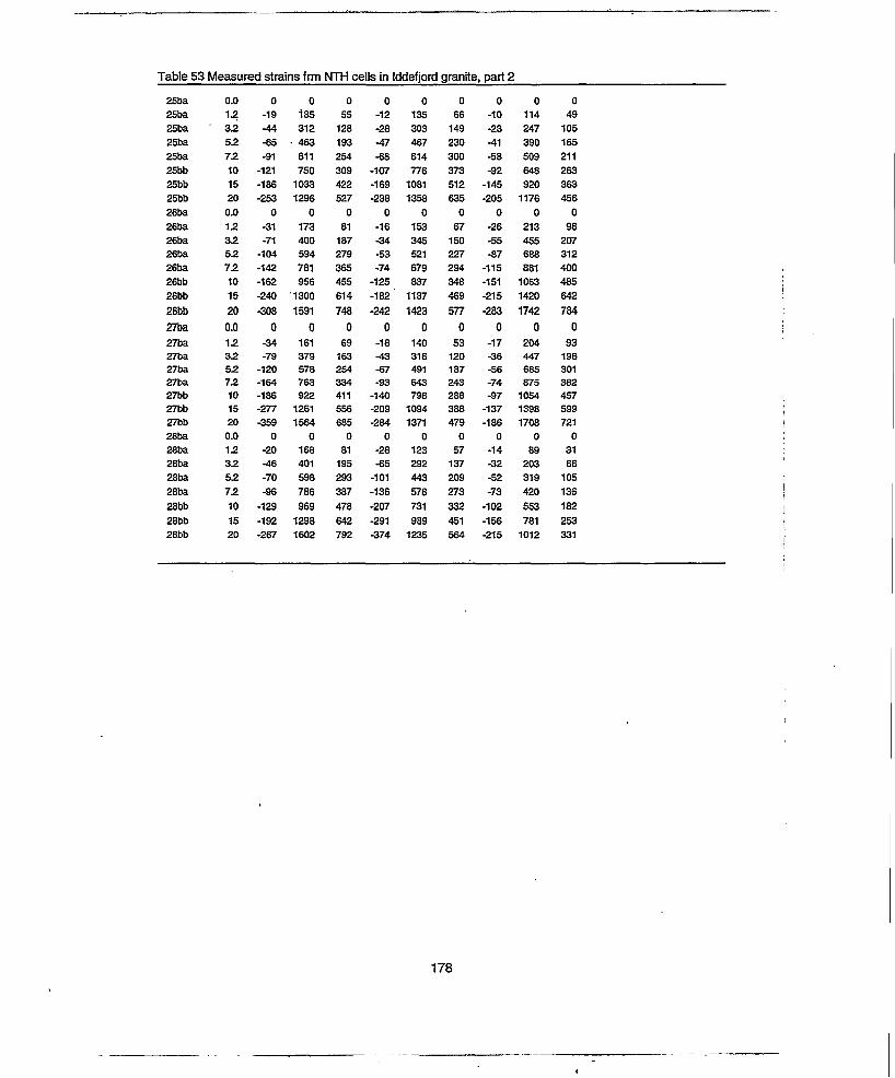
Table 53 Measured strains frm NTH cells in Iddefjord granite, part 2
25ba 0.0 0 0 0 0 0 0 0 0 025ba 12 -19 135 55 -12 135 66 -10 114 4925ba ’ 3 i -44 312 128 -28 303 149 -23 247 10525ba 52 -65 • 463 193 -47 467 230 -41 390 16525ba 72 -91 611 254 -68 614 300 -58 509 21125bb 10 -121 750 309 -107 776 373 -92 648 26325bb 15 -186 1033 422 -169 1081 512 -145 920 36325bb 20 -253 1296 527 -238 1358 635 -205 1176 45626ba 0.0 0 0 0 0 0 0 0 0 026ba 1.2 -31 173 81 -16 153 67 -26 213 9826ba 3.2 -71 400 187 -34 345 150 -55 455 20726ba 52 -104 594 279 -53 521 227 -87 688 31226ba 72 -142 781 365 -74 679 294 -115 881 40026bb 10 -162 956 455 -125 837 348 -151 1063 48526bb 15 -240 1300 614 -182 1137 469 -215 1420 64226bb 20 -308 1591 748 -242 1423 577 -283 1742 78427ba 0.0 0 0 0 0 0 0 0 0 027ba 1.2 -34 161 69 -18 140 53 -17 204 9327ba 35 -79 379 163 -43 316 120 -36 447 19627ba 55 -120 578 254 -67 491 187 -56 685 30127ba 75 -164 763 334 -93 643 243 -74 875 38227bb 10 -186 922 411 -140 796 288 -97 1054 45727bb 15 -277 1261 556 -209 1094 388 -137 1398 59927bb 20 -359 1564 685 -284 1371 479 -186 1708 72128ba 0.0 0 0 0 0 0 0 0 0 028ba 15 -20 168 81 -28 123 57 -14 89 3128ba 32 -46 401 195 -65 292 137 -32 203 6628ba 52 -70 598 293 -101 443 209 -52 319 10528ba 72 -96 786 387 -136 578 273 -73 420 13628bb 10 -129 969 478 -207 731 332 -102 553 18228bb 15 -192 1298 642 -291 989 451 -156 781 25328bb 20 -267 1602 792 -374 1235 564 -215 1012 331
178

Table 54 Measured strains from NTH cells in Larvikite, part 1
Cell Stress 1 2 3 4 5 6 7 8 931 ba 0.0 0 0 0 0 0 0 0 0 031 ba 12 -18 65 24 -25 98 46 -20 64 1431 ba 3 2 -42 154 59 -59 217 99 -43 140 3031ba 5 2 -65 242 93 -92 331 148 -70 230 5131 ba 72 -90 335 130 -127 436 193 -94 310 6931bb 10 -118 440 174 -171 557 239 -131 422 9331 bb 15 -180 665 263 -255 804 343 -195 632 14231 bb 20 -241 902 358 -342 1049 451 -264 842 19232ba 0.0 0 0 0 0 0 0 0 0 032ba 12 -19 66 12 -15 44 13 -18 59 2132ba 32 -47 120 29 -37 109 31 -40 135 4832ba 52 -69 186 46 -58 174 48 -66 220 7932ba 72 -98 266 66 -84 241 65 -93 304 10832bb 10 -128 352 81 -118 319 80 -129 402 13832bb 15 -193 531 122 -183 473 114 -197 607 21032bb 20 -261 705 163 -255 633 143 -277 814 28433ba 0.0 0 0 0 0 0 0 0 0 033ba 12 -20 69 21 -8 60 22 -28 63 1833ba 32 -48 167 50 -19 140 53 -65 141 4133ba 52 -72 259 79 -31 224 85 -105 226 6733ba 72 -100 356 108 -44 306 117 -144 303 9033bb 10 -128 464 139 -66 411 154 -198 399 11533bb 15 -195 686 200 -98 610 231 -310 599 17533bb 20 -265 915 258 -130 822 312 -429 797 23234ba 0.0 0 0 0 0 0 0 0 0 034ba 12 -19 68 25 -21 56 24 -17 91 4034ba 32 -45 158 57 -47 126 55 -39 199 9034ba 52 -68 247 90 -74 201 89 -64 316 13934ba 72 -96 344 125 -101 280 120 -88 419 18234bb 10 -130 452 163 -134 364 155 -127 531 21334bb 15 -198 686 247 -203 536 223 -191 772 30334bb 20 -259 911 334 -278 717 288 -257 999 380
179

Table 55 Measured strains fan NTH cells in Larvikite granite, part 2
35ba 0.0 0 0 0 0 0 0 0 0 035 ba 1.2 -14 67 20 -13 59 19 -25 82 3035ba 3 2 -39 161 47 -32 140 46 -56 187 7135 ba 5 2 -61 253 74 -52 225 76 -90 305 11635ba 72 •-89 348 101 -73 • 305 103 -119 404 15235bb 10 -123 446 123 -31 441 243 -91 568 22935bb 15 -186 670 187 -74 638 320 -162 829 32635bb •20 -245 897 253 -121 842 390 -235 1081 286836ba 0.0 0 0 0 0 0 0 0 0 036ba 1.2 -6 126 69 -14 43 10 -21 80 3536ba 3.2 -16 282 146 -34 100 25 -49 181 7736ba 52 -28 406 201 -54 158 40 -78 287 12336ba 72 -47 524 248 -72 218 56 -105 383 16236bb 10 -74 631 281 -96 298 77 -139 491 20236bb 15 -124 869 364 -143 443 113 -207 726 30336bb 20 -168 1098 446 -194 600 148 -275 959 40137ba 0.0 0 0 0 0 0 0 0 0 037ba 12 -18 71 26 -16 63 18 -16 58 2437ba 32 -44 174 62 -39 151 41 -36 133 5437ba 52 -65 265 96 -62 239 63 -59 213 8737ba 72 -93 372 136 -88 330 87 -82 288 11637bb 10 -119 489 186 -131 440 109 -116 390 15637bb 15 -180 725 276 -191 647 160 -177 576 22737bb 20 -240 972 363 -249 869 210 -243 767 30038ba 0.0 0 0 0 0 0 0 0 0 038ba 12 -19 62 17 -19 101 1 -19 69 3638ba 32 -51 156 43 -51 233 5 -46 157 7938ba 52 -78 243 67 -83 356 10 -74 253 12638ba 72 -113 341 95 -119 475 16 -102 339 16538bb 10 -151 453 128 -191 572 18 -140 449 22138bb 15 -234 675 192 -300 838 28 -217 665 31238bb 20 -337 909 247 -383 1081 50 -300 878 400
180

Table 56 Measured strains from NTH cells in Ftoyken granite, part 1
Cell Stress 1 2 3 4 5 6 7 8 911ba 0.0 0 0 0 0 0 0 0 0 011ba 12 13 47 14 -36 144 48 -44 116 4511ba 32 24 82 19 -87 351 119 -68 197 7911ba 52 31 127 25 -146 592 208 -129 320 11811ba 72 38 155 27 -179 717 249 -144 360 12611bb 10 -11 209 -13 -194 1012 382 -210 473 17811bb 15 -53 301 -4 -283 1325 492 -280 602 19411bb 20 -71 344 6 -364 1633 600 -354 728 21412ba 0.0 0 0 0 0 0 0 0 0 012ba 12 -8 104 48 -17 253 111 -19 115 4812ba 32 -20 255 116 -36 485 212 -47 264 10712ba 52 -26 389 180 -52 685 301 -82 422 16812ba 72 -45 549 247 -72 875 377 -115 553 21612bb 10 -55 682 305 -114 1056 442 -163 702 26512bb 15 -94 970 423 -156 1400 573 -240 961 35712bb 20 -133 1253 543 -195 1724 695 -325 1223 44113ba 0.0 0 0 0 0 0 0 0 0 013ba 12 -33 123 63 -34 192 56 -20 105 6113ba 32 -80 300 150 -68 424 130 -41 240 17813ba 52 -114 . 446 224 -100 629 201 -64 400 23113ba 72 -160 612 301 -124 813 262 -69 526 29713bb 10 -152 745 384 -188 982 299 -104 667 36713bb 15 -223 1033 521 -266 1307 410 -151 931 50513bb 20 -294 1318 651 -351 1610 506 -202 1184 831I4ba 0.0 0 0 0 0 0 0 0 0 014ba 12 -31 284 77 -30 110 41 6 117 6114ba 32 -78 573 152 -76 259 94 7 270 13814ba 52 -112 804 217 -124 404 143 0 431 20514ba 72 -154 1019 277 -174 543 189 -4 569 26414bb 10 -205 1155 298 -196 723 264 -38 706 28214bb 15 -280 1490 399 -298 1005 365 -67 972 36914bb 20 -348 1825 500 -400 1275 467 -105 1246 447
181

Table 57 Measured strains from NTH cells in Rgyken granite, part 2
15ba 0.0 0 0 0 0 0 0 0 0 015ba 1.2 -23 386 158 -32 125 70 -29 170 5815ba 3.2 -61 753 297 -67 ' 271 143 -58 342 11315ba 52 -93 1024 398 -102 406 211 -87 508 16715ba ' 72 -137 1279 485 -140 536 272 -114 649 20815bb 10 -190 1475 543 -187 689 344 -152 798 25615bb 15 -293 1929 697 -287 975 468 -211 1084 33615bb 20 -384 2349 835 -400 1260 588 -271 1375 42016ba 0.0 0 0 0 0 0 0 0 0 016ba 12 -42 152 51 -36 251 117 -28 303 016ba 32 -96 356 121 -69 487 224 -54 606 016ba 52 -143 528 178 -95 675 307 -82 889 016ba 72 -196 703 232 -117 830 371 -107 1117 016bb 10 -197 852 286 -151 946 391 -131 1438 86316bb 15 -283 1163 388 -201 1202 482 -191 1832 108916bb 20 -359 1444 481 -249 1440 562 -259 2219 130617ba 0.0 0 0 0 0 0 0 0 0 017ba 1.2 -9 305 134 -19 84 39 -11 197 10517ba 32 -30 606 266 -48 202 90 -25 398 19917ba 52 -44 820 361 -75 318 139 -45" 580 28417ba 72 -62 1022 447 ' -102 438 184 -63 741 350I7bb 10 -99 1205 506 -117 564 241 -101 904 413I7bb 15 -138 1568 655 -167 839 349 -156 1233 557I7bb 20 -164 1895 789 -213 1114 457 -225 1562 69618ba 0.0 0 0 0 0 0 0 0 0 018ba 12 -12 109 38 -23 255 113 -18 151 5518ba 32 -34 247 86 -56 500 211 -42 333 12818ba 52 -54 378 132 -92 702 290 -69 515 19618ba 72 -79 509 178 -129 868 351 -93 665 24918bb 10 -111 636 225 -179 1026 399 -131 830 30218bb 15 -176 930 331 -271 1367 517 -204 1161 41518bb 20 -236 1191 429 -357 1679 625 -286 1488 524
182

Table 58 Measured strains by NTH cells during axial stressing of hollow aluminum cylinders
O. e, Gz Gj0.0 0 0 02.7 24 -5 85.4 48 -13 1210.8 105 -31 3116.3 167 -52 5221.7 233 -74 7427.1 301 -96 970.0 4 5 5
0.0 0 0 02.7 0 -1 25.4 8 -3 610.8 46 -15 2316.3 102 -32 4521.7 168 -52 6927.1 238 -74 940.0 .1 1 2
0.0 0 0 02.7 12 -9 65.4 40 -17 2110.8 106 -34 4816.3 172 -54 7421.7 241 -75 9927.1 311 -97 1240.0 1 2 1
0.0 0 0 02.7 75 -10 245.4 141 -28 4510.8 257 -58 8416.3 363 -85 11621.7 445 -108 14427.1 521 -131 1690.0 25 23 22
e5. e6 G, e» Gg0 0 0 0 0-15 11 27 -8 9;29 21 61 -18 19-51 42 131 -43 41-73 67 199 -66 63-94 93 265 -89 83-116 118 331 -111 1044 4 1 3 3
0 0 0 0 0-12 5 62 -21 17-21 8 125 -41 36-39 15 235 -77 71-58 29 329 -106 103-79 48 415 -133 132-101 68 496 -158 1601 2 2 1 1
0 0 0 0 0-12 5 52 -24 8-19 18 104 -36 27-38 42 191 -62 53-60 68 272 -86 80-83 94 347 -110 104-107 122 423 -133 1291 7 0 3 2
0 0 0 0 0-7 27 17 -1 3-16 55 36 -3 11-35 103 74 -5 20-56 137 131 -22 39-78 166 199 -41 62-100 193 271 -61 8719 17 18 13 17
e.o55991732443163884
037671211782423091
016471141842583331
0479218025833240520
183

Table 59 Measured strains from NTH cells during radial stressing of hollow steel cylinders.
Cell o. G, Gj e, e< G, e6 e. Ga Gg -1.1 0 0 0 0 O 0 0 0 0 0
3.2 -13 44 15 -14 43 16 -10 42 1482. -37 118 41 -38 120 42 -31 117 3913 2 -61 196 67 -62 193 67 -50 189 6218 2 -84 268 92 -86 266 92 -70 259 8523 2 -107 339 116 -109 336 117 -88 328 10828 2 -129 411 141 -132 409 142 -107 399 1320 2 2 1 1 1 2 1 1 1
1.2 0 0 0 0 0 0 0 0 0 03 2 -10 51 20 -13 50 19 -10 49 2082 -31 124 46 -36 122 45 -29 120 4613 2 -53 199 74 -61 196 71 -49 194 7318 2 -74 274 100 -85 271 97 -70 268 10123 2 -94 346 126 -109 341 123 -89 338 128282 -115 420 153 -132 413 149 -108 411 1560 13 13 12 13 12 11 12 12 11
1.3 0 0 0 0 0 0 0 0 0 03 2 -16 48 14 -13 48 18 -13 49 1982 -44 117 35 -33 119 44 -36 120 46132 -73 190 56 -54 192 72 -59 194 74182 -102 260 77 -75 264 98 -81 268 102232 -130 331 97 -96 336 124 -104 341 13128 2 -157 400 118 -116 406 150 -126 413 1590 7 5 4 5 4 4 5 4 4
1.4 0 0 0 0 0 0 0 0 0 032 -16 44 15 -11 49 19 -12 48 1882 -40 107 34 -33 119 43 -32 118 44132 -66 173 53 -55 192 69 -53 190 70182 -91 238 73 -78 264 94 -74 262 97232 -116 303 92 -100 337 120 -95 335 125282 -140 365 111 -122 408 145 -115 407 1520 -1 1 1 2 2 2 1 2 1
2.1 0 0 0 0 0 0 0 0 0 032 -15 45 17 -19 46 14 -15 48 1782 -36 117 43 -47 116 36 -36 117 41132 -56 186 68 -74 186 58 -59 192 68182 -78 263 95 -104 261 81 -81 265 93232 -97 330 120 -135 329 102 -103 338 120282 -117 399 144 -161 393 122 -122 402 1430 -1 -3 0 -1 0 1 -1 0 0
2.2 0 0 0 0 0 0 0 0 0 032 -59 136 41 -12 38 2 -54 141 4582 -141 342 104 -8 100 -3 -131 334 104132 -220 543 169 -14 166 8 -211 555 178182 -305 753 237 -5 233 9 -288 756 2440 -11 -36 -15 -28 -17 -22 -12 -18 -6
2.3 0 0 0 0 0 0 0 0 0 032 -13 47 18 -17 48 15 -13 48 1682 -33 120 44 -41 118 38 -32 116 39132 -55 193 71 -67 193 64 -53 193 66182 -76 269 98 -93 268 88 -73 264 90232 -95 336 122 -116 336 ' 112 -93 334 114282 -119 408 148 -140 406 135 -113 400 1360 3 -1 1 0 0 -1 3 0 1
184

Table 60 Measured strains from NTH cells during radial stressing of hollow aluminum cylinders
Cell e; e= e. e5 e6 G? Ge Gg
1.2 0 0 0 0 0 0 0 0 0 03 2 -58 152 46 -59 148 45 -53 ' 145 4482 -136 361 110 -140 .357 109 -129 357 10913 2 -224 587 177 -224 570 174 -202 556 1690 0 1 0 -2 -1 -1 -1 -1 -2
1.3 0 0 0 0 0 0 0 . 0 0 03 2 -52 152 49 -54 148 46 -51 150 5582 -136 372 118 -132 359 111 -120 358 13013 2 -208 587 184 -207 575 179 -196 585 2120 9 10 10 8 9 9 8 10 10
1.4 0 0 0 0 0 0 0 0 0 032 -58 155 52 -50 152 52 -42 156 6082 -134 367 121 -125 365 121 ■ -114 378 13413 2 -224 602 193 -205 584 191 -183 591 20718 2 -286 794 255 -272 782 258 -253 803 2800 14 17 17 16 17 18 19 21 23
2.1 0 0 0 0 0 0 0 0 0 032 -53 142 44 -61 142 41 -49 138 4282 -127 348 110 -151 357 104 -124 352 10713 2 -207 562 177 -242 573 167 -197 . 557 16918 2 -276' 756 244 -331 787 231 -274 779 2370 0 1 0 0 0 0 -1 1 0
22 0 0 0 0 0 0 0 0 0 032 -59 136 41 -12 38 2 -54 141 4582 -141 342 104 -8 100 -3 -131 334 10413 2 -220 543 169 -14 166 8 -211 555 17818 2 -305 753 237 -5 233 9 -288 756 2440 -11 -36 -15 -28 -17 -22 -12 -18 -6
2.3 0 0 0 0 0 0 0 0 0 032 -74 130 28 -S3 139 30 - -77 132 3482 -151 336 99 -168 344 92 -149 334 10413 2 -225 544 174 -257 567 159 -229 560 18418 2 -307 759 249 -344 791 225 -295 743 2400 -19 -17 -21 -21 -10 -15 -21 -18 -17
2.4 0 0 0 0 0 0 0 0 0 032 -60 131 42 -59 145 42 -52 81 3582 -133 294 98 -135 343 102 -122 206 9113 2 -223 489 163 -219 565 169 -195 329 1480 -4 -8 -4 -5 -6 -6 -6 -19 -6
I
i
i
185
T7TTT-

Table 61 Measured strains from NTH cells during radial loading
o«4.8
12.8
19.9
27.5
35.0
42.5
Cell e, e. e, e. e5 e6 e. Ga1.1 -13 44 15 -14 43 16 -10 42 141.2 -10 51 20 -13 50 19 -10 49 201.3 -16 48 14 -13 48 18 -13 49 191.4 -16 44 15 -11 49 19 -12 48 182.1 -15 45 17 -19 46 14 -15 48 1722. -13 51 20 -17 33 12 -17 50 182.3 -13 47 18 -17 48 15 -13 48 161.1 -37 118 41 -38 120 42 -31 117 3912 -31 124 46 -36 122 45 -29 120 461.3 -44 117 35 -33 119 44 -36 120 461.4 -40 107 34 -33 119 43 -32 118 442.1 -36 117 43 -47 116 36 -36 117 4122 -34 121 46 -38 81 24 -35 116 432.3 -33 120 44 -41 118 38 -32 116 391.1 -61 196 67 -62 193 67 -50 189 6212 -53 199 74 -61 196 71 -49 194 731X3 -73 190 56 -54 192 72 -59 194 741.4 -66 173 53 -55 192 69 -53 190 702.1 -56 186 68 -74 186 58 -59 192 6822 -54 195 73 -63 133 41 -58 193 702.3 -55 -• 193 71 -67 193 64 -53 193 661.1 -74 268 92 -85 266 92 -70 259 8512 -84 274 100 -86 271 97 -70 268 1011.3 -102 260 77 -75 264 98 -81 268 1021.4 -91 238 73 -78 264 94 -74 262 972.1 -78 263 95 -104 261 81 -81 265 9322 -79 271 101 -85 182 54 -78 263 962.3 -76 269 98 -93 268 88 -73 264 901.1 -107 339 116 -109 336 117 -88 328 10812 -94 346 126 -109 341 123 -89 338 1281.3 -130 331 97 -96 336 124 -104 341 1311.4 -116 303 92 -100 337 120 -95 335 1252.1 -97 330 120 -135 329 102 -103 338 12022 -97 341 127 -107 231 71 -100 337 12222 -95 336 122 -116 336 112 -93 334 1141.1 -129 411 141 -132 409 142 -107 399 13212 -115 420 153 -132 413 149 -108 411 1561.3 -157 400 118 -116 406 150 -126 413 1591.4 -140 365 111 -122 408 145 -115 407 1522.1 -117 399 144 -161 393 122 -122 402 14322 -121 416 154 -129 279 84 -119 405 1472.3 -119 408 148 -140 406 135 -113 400 136
186

Table 62 Results from leak-off-tests (LOT) and formation integrity tests (FIT)
WELL NO. DEPTH[mRKBTVD]
PrT[MPa]
Plot[MPa]
34/8-1 959 15.7 .34/8-1 1773 30.1 -
34/8-1 2379 43.2 -
34/8-2 1177 - 18.834/8-2 2680 - 48.234/8-3 1302 - 21.234/8-3 2597 - 48.334/8-3A 944 15.7 17.434/8-3A 2342 - 43.034/8-4S 1167 - 18.434/8-4S 2161 - 38.434/8-4S 3740 - 77.434/8-5 1197 18.3 -
34/8-5 2612 47.5 -
34/8-7 1440 - 23.334/8-7 3285 - 62.034/8-7 3958 - 79.134/8-8 1367 22.6 -
34/8-8 2768 50.3 -
34/8-9S 1363 . 21.134/8-9S 2470 - 44.4
187

Table 63 Results from minifrac testing in selected Visund wells
WELL NO. DEPTH P, Pp Ps Pc TEST.NO[mRKBTVD] [MPa] [MPa] [MPa] [MPa]
.34/8-3 2895.79 60.5 58.8 _ _ 134/8-3 2850.11 56.8 54.2 52.7 51.4 2'34/8-3 2825.56 59.5 58.3 57.0 56.3 334/8-3A 2933.7 57.6 - 53.8 53.3 134/8-7R 5027.8 107.6 101.9 97.2 95.6 134/8-7R 4566.7 96.5 87.7 85.9 85.0 234/8-8R 2941.8 72.9 56.4 55.0 54.5 134/8-8R 2910.6 73.4 61.1 61.0 60.4 2
188