investigations of helium transport in asdex upgrade plasmas … · fates warning - monument. a...
TRANSCRIPT

Investigations of helium transport in ASDEX
Upgrade plasmas with charge exchange
recombination spectroscopy
PROEFSCHRIFT
ter verkrijging van de graad van doctor aan de
Technische Universiteit Eindhoven, op gezag van de
rector magnificus prof.dr.ir. C.J. van Duijn, voor een
commissie aangewezen door het College voor
Promoties, in het openbaar te verdedigen op
donderdag 23 oktober 2014 om 16:00 uur
door
Athina Kappatou
geboren te Thessaloniki, Griekenland

Dit proefschrift is goedgekeurd door de promotoren en de samenstelling van de
promotiecommissie is als volgt:
voorzitter: prof.dr.ir. G.M.W. Kroesen
promotor: prof.dr. A.J.H. Donne
copromotoren: dr. R.J.E. Jaspers
dr. R.M. McDermott (Max-Planck-Institut fur Plasmaphysik)
leden: dr. W. Biel (Forschungszentrum Julich)
prof.dr. R.J. Fonck (University of Wisconsin-Madison)
prof.dr. W.W. Heidbrink (University of California)
prof.dr.ir. O.J. Luiten

Investigations of helium transport in ASDEX
Upgrade plasmas with charge exchange
recombination spectroscopy
by
Athina Kappatou
to my parents
Is it fiction, is it confession?
Is it passion or just a profession?
Is it performance, is it expression?
Is it passion or just an obsession?
Fates Warning - Monument

A catalogue record is available from the Eindhoven University of Technology
Library
Kappatou, Athina
Investigations of helium transport in ASDEX Upgrade plasmas with charge
exchange recombination spectroscopy
ISBN: 978-90-386-3704-4
NUR: 926
This work is part of the research programme of the Foundation for Fundamental
Research on Matter (FOM), which is part of the Netherlands Organisation for
Scientific Research (NWO).
This work has been carried out within the framework of the EUROfusion
Consortium and has received funding from the European Unions Horizon 2020
research and innovation programme under grant agreement number 633053.
The views and opinions expressed herein do not necessarily reflect those of the
European Commission.
Cover design: “Purple and Teal”, by Matthias Bernert, with contributions from
Athina Kappatou and Andreas Burckhart
c�2014, Athina Kappatou

Contents
Summary iii
Samenvatting vii
Zusammenfassung xi
1 Introduction 1
1.1 Nuclear fusion . . . . . . . . . . . . . . . . . . . . . . . . . . . . . . . . . 1
1.2 The role of helium in a fusion plasma . . . . . . . . . . . . . . . . . . . . 3
1.3 This thesis . . . . . . . . . . . . . . . . . . . . . . . . . . . . . . . . . . . 4
2 The ASDEX Upgrade tokamak 7
2.1 Tokamak operation . . . . . . . . . . . . . . . . . . . . . . . . . . . . . . 7
2.2 Plasma heating systems on ASDEX Upgrade . . . . . . . . . . . . . . . 11
2.3 Plasma diagnostics on ASDEX Upgrade . . . . . . . . . . . . . . . . . . 15
3 Charge exchange recombination spectroscopy 25
3.1 Components of a charge exchange spectrum . . . . . . . . . . . . . . . . 26
3.2 Charge exchange recombination spectroscopy as a
plasma diagnostic . . . . . . . . . . . . . . . . . . . . . . . . . . . . . . . 36
3.3 CXRS diagnostic instrumentation at ASDEX Upgrade . . . . . . . . . 44
4 Impurity transport theory 53
4.1 Radial impurity transport . . . . . . . . . . . . . . . . . . . . . . . . . . 54
4.2 Neoclassical impurity transport . . . . . . . . . . . . . . . . . . . . . . . 55
4.3 Turbulent transport . . . . . . . . . . . . . . . . . . . . . . . . . . . . . 62
4.4 Experimental studies on helium confinement, exhaust and recycling . . . 72
5 The helium plume e↵ect 75
5.1 The helium plume emission . . . . . . . . . . . . . . . . . . . . . . . . . 76
5.2 Modelling of the helium plume emission . . . . . . . . . . . . . . . . . . 80
i

CONTENTS
5.3 Dependence of the helium plume emission on plasma parameters and
diagnostic characteristics . . . . . . . . . . . . . . . . . . . . . . . . . . . 88
5.4 Experimental investigation of the helium plume e↵ect . . . . . . . . . . 104
5.5 Reconstruction of the helium spectrum . . . . . . . . . . . . . . . . . . . 109
5.6 Considerations on the plume e↵ect . . . . . . . . . . . . . . . . . . . . . 113
6 Investigation of the thermal helium transport in ASDEX Upgrade
plasmas 117
6.1 Database for the investigation of helium transport . . . . . . . . . . . . 119
6.2 Experimental observations . . . . . . . . . . . . . . . . . . . . . . . . . . 122
6.3 Comparison to impurity transport theory . . . . . . . . . . . . . . . . . 123
6.4 Conclusions . . . . . . . . . . . . . . . . . . . . . . . . . . . . . . . . . . 144
7 Feasibility of charge exchange measurements of slowing down alpha
particles on ITER 147
7.1 Fast ion charge exchange diagnostic technique . . . . . . . . . . . . . . . 149
7.2 Simulation package for charge exchange spectroscopy . . . . . . . . . . . 151
7.3 Simulation of the non-thermal helium charge exchange spectrum . . . . 153
7.4 Discussion . . . . . . . . . . . . . . . . . . . . . . . . . . . . . . . . . . . 161
7.5 Feasibility of charge exchange measurements of the helium “ash” on ITER165
8 Conclusions and outlook 169
8.1 Helium transport investigations at ASDEX Upgrade . . . . . . . . . . . 170
8.2 Outlook . . . . . . . . . . . . . . . . . . . . . . . . . . . . . . . . . . . . 173
Appendices 175
A Impurity density profiles combining CXRS and BES 177
B E↵ect of sawtooth crashes on the thermal helium profile 185
C Feasibility of energetic helium studies at ASDEX Upgrade 187
Acknowledgements 189
Curriculum Vitae 191
Symbols and acronyms 193
List of Figures 197
References 201
ii

Summary
Investigations of helium transport in ASDEX Upgrade plasmas with
charge exchange recombination spectroscopy
Nuclear fusion is the merging of two light nuclei to form a heavier one; a process that
can release significant amounts of energy. One does not have to look very hard to find
fusion reactions. The sun, for example, is powered by fusion processes. Harnessing fu-
sion reactions on earth for commercial energy production is the subject of fusion energy
research. However, for the two nuclei to fuse, they must first be brought su�ciently
close together so that the nuclear Strong force overcomes the Coulomb repulsion. This
requires very high temperatures (hundreds of millions of degrees Celsius), meaning that
the fusion “fuel” is ionised, forming a plasma. One of the most extensively explored
ways to confine such a plasma on earth is the tokamak, which is a torus shaped device
with a helical magnetic field that is employed to keep the plasma particles confined
and prevent them from impinging on the tokamak wall. ITER, the international ex-
perimental fusion reactor, will be a tokamak.
The most promising fusion reaction for fusion energy production on earth, the
deuterium-tritium reaction, leads to the production of helium, which carries 3.5MeV of
kinetic energy (one fifth of the total produced energy). Understanding the behaviour
of the helium in a future fusion reactor is critical for its performance. The fusion pro-
duced helium is needed to heat the plasma through collisions with the plasma particles.
However, it is thermalised in this process, leaving (without a loss mechanism) a con-
tinuously increasing thermalised helium content in the plasma as the fusion reactions
continue to take place. This increasing helium population causes dilution of the fusion
fuel and stifles the fusion reactions. This so-called helium “ash” has to be removed
iii

CONTENTS
from the plasma core. It is, therefore, of great importance to understand and control
the helium in a fusion plasma.
The helium in the plasma can be studied with charge exchange recombination spec-
troscopy, a diagnostic method which is based on the exchange of an electron between
a neutral particle and a plasma impurity ion (e.g. helium). The impurity ion, after
obtaining the electron, emits characteristic line radiation that contains key informa-
tion on the impurity species. Charge exchange recombination spectroscopy provides
spatially and temporally resolved measurements of impurity temperature, rotation and
density in the plasma. This thesis attempts to shed light on the transport properties of
helium in fusion plasmas, using charge exchange spectroscopy. A high etendue charge
exchange spectrometer was installed and utilised for the helium measurements at the
ASDEX Upgrade tokamak.
Helium charge exchange measurements are, however, hindered by the so-called
“plume” e↵ect, an additional emission which is comparable to the charge exchange
signal. Accurate helium density profiles can be derived from the measurements only if
the plume emission is modelled and subtracted from the measured spectra. For this
reason, a model that takes into account the diagnostic observation geometry, the recon-
structed magnetic equilibrium, appropriate atomic data, and involves a Monte Carlo
approach to describe the velocity distribution of the plume ions was implemented at
ASDEX Upgrade and benchmarked against experimental measurements. The model is
shown to describe the underlying physics mechanisms accurately, as it can reproduce
the experimental helium spectra, enabling accurate ion temperatures and rotations to
be extracted from the data. Not only the plume to prompt emission intensity ratio is
provided, but also the plume spectral emission line and its non-Maxwellian features are
reconstructed.
With the confidence that accurate helium density profiles can now be derived from
charge exchange measurements, investigations of helium transport have been under-
taken at ASDEX Upgrade. To this end, a database of experimental measurements of
helium and boron density profiles was assembled via specially designed experiments.
The helium density profiles were found to follow closely the electron density profiles,
while clear di↵erences are observed between the helium and boron density profiles. To
try and understand the experimental observations, these measurements were compared
to the available theoretical predictions of both neoclassical and turbulent transport.
iv

CONTENTS
The neoclassical contributions were found to be small or negligible in the investigated
region of the plasma. Rather, turbulent transport, as calculated via linear gyrokinetic
modelling, was found to be the dominant mechanism. Qualitative agreement between
the experiment and the turbulent transport predictions was found under certain con-
ditions. However, cases were also found in which strong disagreements are observed.
Further work on the theoretical side is motivated by these results, as knowing how
the helium density profile will behave in future fusion reactors will be critical for their
successful operation. Understanding of the helium transport in fusion plasmas and
experimental validation of the theoretical understanding are required.
Charge exchange recombination spectroscopy is expected to provide ion tempera-
ture, rotation and helium “ash” measurements on ITER and can also provide some
information on the fusion-produced, slowing-down helium. A study on the feasibility of
such measurements using the reference design of ITER CXRS diagnostic shows that the
signal-to-noise ratio of the slowing-down helium measurements will be very low. Never-
theless, by combining measurements on both the diagnostic and heating neutral beams
on ITER, ↵ particles with energies of up to 1MeV can be diagnosed, though with lim-
ited time and energy resolution. Higher optical throughput instrumentation will help
in this regard, but the optics on the torus side pose a limit on the signal-to-noise ratio
that can be achieved.
In conclusion, at ASDEX Upgrade a helium plume model has been implemented
that for the first time is shown to be able to accurately reproduce the experimental
spectra and enables helium transport studies to be performed via CXRS measurements.
Experimental investigations have been undertaken at ASDEX Upgrade, which present
the first steps towards a better understanding of helium transport in fusion plasmas.
v


Samenvatting
Onderzoek naar heliumtransport op ASDEX Upgrade met CXRS
Kernfusie is het samenvoegen van twee lichte atoomkernen tot een zwaardere; een pro-
ces dat een significante hoeveelheid energie vrijzet. Het is niet moeilijk in de natuur
fusiereacties te vinden. Zo wordt bijvoorbeeld de energie van de zon opgewekt in
fusieprocessen. Het onder controle krijgen van fusiereacties op aarde voor commerciele
energieopwekking is het onderwerp van fusieonderzoek. Om twee atoomkernen te laten
fuseren moeten ze echter eerst voldoende dicht bij elkaar gebracht worden, zodat de
sterke kernkracht de afstotende Coulombkracht overwint. Hiervoor zijn zeer hoge tem-
peraturen nodig (honderden miljoenen graden Celsius), waardoor de “fusiebrandstof”
geıoniseerd raakt en een plasma vormt. Een van de meest onderzochte manieren om
een dergelijk plasma op aarde op te sluiten is de tokamak; een torusvormige machine
met een helisch magnetisch veld dat de plasmadeeltjes opsluit en voorkomt dat deze de
wand raken. ITER, de internationale experimentele fusiereactor, zal een tokamak zijn.
De meest veelbelovende fusiereactie voor energieproductie op aarde, de deuterium-
tritium reactie, resulteert in de productie van helium met 3.5MeV kinetische energie
(een vijfde van de totale geproduceerde energie). Het begrijpen van het gedrag van
dit helium in toekomstige fusiereactoren is cruciaal. Het door fusie geproduceerde he-
lium is nodig om het plasma te verhitten, door botsingen met de plasma-elektrons en
plasma-ionen. Het helium koelt af in dit proces, waardoor de hoeveelheid afgekoeld
helium continu toeneemt naarmate er meer fusiereacties plaatsvinden, als de verlies-
mechanismes buiten beschouwing worden gelaten. Deze zogenaamde “helium-as” moet
uit het plasmacentrum verwijderd worden. Het is daarom zeer belangrijk helium trans-
port in een fusiereactor te begrijpen en te controleren.
vii
CONTENTS
Het helium in het plasma kan onderzocht worden met CXRS (‘Charge eXchange Re-
combination Spectroscopy’), een diagnostische methode die gebaseerd is op de uitwissel-
ing van een elektron tussen een neutraal deeltje en een verontreinigings-ion (bijv. he-
lium). De lijnstraling die het verontreinigings-ion uitzendt na het ontvangen van het
elektron bevat belangrijke informatie over de eigenschappen van de verontreinigin-
gen. CXRS geeft in ruimte en tijd opgeloste metingen van de temperatuur, rotatie
en dichtheid van de verontreinigingen. Dit proefschrift probeert licht te werpen op
de transporteigenschappen van helium in fusieplasmas. Hiervoor is een CXRS spec-
trometer voor helium metingen en met een hoge “etendue” geinstalleerd op de ASDEX
Upgrade tokamak.
Helium CXRS-metingen worden echter bemoeilijkt door het zogenaamde plume-
e↵ect, een additionele stralingsproces die vergelijkbaar in amplitude is met het CXRS-
signaal. Nauwkeurige profielen van de heliumdichtheid kunnen enkel uit de metingen
worden afgeleid als het plume-e↵ect wordt gemodelleerd en van de metingen wordt
afgetrokken. Om deze reden is op ASDEX Upgrade een model ontwikkeld dat reken-
ing houdt met de observatiegeometrie, het gereconstrueerde magnetische evenwicht, de
benodigde atomaire data en een Monte-Carlo simulatie om de snelheidsverdeling van
de plume-ionen te beschrijven. Dit model is vergeleken met experimentele metingen.
Het is aangetoond dat dit model de onderliggende fysische mechanismen nauwkeurig
beschrijft, aangezien het de experimentele heliumspectra reproduceert. Dit maakt het
mogelijk de ionentemperatuur en rotatie nauwkeurig uit de data af te leiden. Naast
de verhouding tussen het plume-e↵ect en de directe stralingsintensiteit wordt ook de
spectrale emissielijn van het plume-e↵ect met zijn niet-Maxwellse eigenschappen gere-
construeerd.
Met het vertrouwen dat de helium-dichtheidsprofielen nauwkeurig uit de CXRS-data
kunnen worden afgeleid is onderzoek naar het heliumtransport op ASDEX Upgrade uit-
gevoerd. Hiervoor is aan de hand van speciaal ontworpen experimenten een database
van experimenteel gemeten helium- een boor-dichtheidsprofielen aangelegd. Het is
gebleken dat de helium-dichtheidsprofielen de elektronen-dichtheidsprofielen nauwkeurig
volgen, terwijl er grote verschillen met de boor-dichtheidsprofielen waargenomen wor-
den. Om deze experimentele observaties te verklaren zijn de metingen vergeleken met
de beschikbare theoretische voorspellingen van zowel het neoklassieke en turbulente
viii
transport. De neoklassieke bijdrages bleken klein of verwaarloosbaar te zijn in het on-
derzochte plasmagebied. Turbulent transport daarentegen, zoals berekend met lineaire
gyrokinetische modellen, bleek het dominante transportmechanisme. Onder bepaalde
voorwaarden werd een kwalitatieve overeenstemming tussen het experiment en de mod-
elvoorspellingen voor turbulent transport gevonden. In andere gevallen werden echter
ook grote afwijkingen waargenomen. Deze resultaten moedigen aan meer theoretisch
werk te verrichten, aangezien het kennen van het gedrag van helium-dichtheidsprofielen
cruciaal is voor het succesvol bedrijven van toekomstige fusiereactoren. Begrip van het
heliumtransport in fusieplasmas en een experimentele bevestiging van de theoretische
modellen is noodzakelijk.
CXRS zal op ITER metingen van de ionentemperatuur, rotatie en “helium-as” lev-
eren, en kan ook informatie leveren over het door fusie geproduceerde snelle “slowing-
down” helium. Uit onderzoek naar de haalbaarheid van zulke metingen, gebruikmakend
van het referentieontwerp van ITER-CXRS, is gebleken dat de signaal-ruisverhouding
van metingen van het snelle helium zeer laag zal zijn. Desalniettemin kunnen door het
combineren van metingen aan de verschillende neutrale bundels op ITER (voor verhit-
ting en als diagnostiekbundel) ↵-deeltjes met een energie tot 1MeV gemeten worden,
weliswaar met beperkte tijds- en energieresolutie. Instrumentatie met een hogere lich-
topbrengst zal in dit opzicht helpen, maar de optica aan de toruszijde begrenst de te
bereiken signaal-ruisverhouding.
Conclusie: op ASDEX Upgrade is een plume-model voor helium geımplementeerd
dat voor het eerst in staat is de experimentele spectra nauwkeurig te reproduceren, en
zo de studie van heliumtransport met CXRS-metingen mogelijk maakt. Het verrichte
experimenteel onderzoek op ASDEX Upgrade is de eerste stap in de richting van een
beter begrip van heliumtransport in fusieplasmas.


Zusammenfassung
Untersuchungen des Helium-Transports mit CXRS an ASDEX
Upgrade Plasmen
Die Kernfusion ist das Verschmelzen von zwei leichten Atomkernen zu einem schwe-
reren Kern: ein Prozess bei dem erhebliche Energiemengen freigesetzt werden konnen.
Solche Fusionsreaktionen finden auch in der Natur statt. So produziert z.B. die Sonne
ihre Energie durch die Fusion von Wassersto↵. Fusionsforschung versucht Fusionreak-
tionen auf der Erde fur kommerzielle Energieproduktion nutzbar zu machen. Um die
zwei Kerne zu verschmelzen mussen sie jedoch sehr nahe zusammengebracht werden,
damit die starke Wechselwirkung die abstoßende Coulomb-Kraft ubersteigt. Dazu sind
sehr hohe Temperaturen notwendig (mehrere Millionen Grad Celsius), was bedeutet,
dass der Fusionskraftsto↵ ionisiert ist und ein Plasma bildet. Der besterforschteste Weg
ein Fusionsplasma einzuschließen ist der Tokamak, ein torusformiges Gerat mit einem
helikalen Magnetfeld, welches die Plasmateilchen einschließt und verhindert, dass diese
an die Wand des Tokamaks stoßen. ITER, der internationale experimentelle Fusionsre-
aktor, wird ein Tokamak sein.
Die vielversprechendste Fusionsreaktion fur die Energieproduktion auf der Erde,
die Fusion von Deuterium und Tritium, fuhrt zu der Produktion eines Heliumkerns,
der eine kinetische Energie von 3.5MeV tragt (ein Funftel der gesamten produzierten
Energie einer Fusionsreaktion). Das Verstandnis des Verhaltens von Helium in einem
zukunftigen Fusionsreaktor ist fur dessen Erfolg entscheidend. Das Helium, welches
durch die Fusionsreaktion produziert wird, soll das Plasma durch Stoße mit den Plas-
mateilchen heizen. Hierdurch nimmt das Helium die Plasmatemperatur an, was ohne
einen Verlustmechanismus zu einem stetig ansteigenden Gehalt von thermalisiertem
Helium im Plasma fuhren wurde, wahrend die Fusionsreaktionen stattfinden. Diese
xi

CONTENTS
stetig ansteigende Helium-Konzentration wurde den Fusionskraftsto↵ verdunnen und
die Fusionsreaktion unterdrucken. Die sogenannte Helium-Asche muss aus dem Plas-
makern entfernt werden. Deswegen sind das Verstandnis und die Kontrolle von Helium
in einem Fusionsplasma von großer Bedeutung.
Das Helium in dem Plasma kann mit Hilfe von Ladungsaustauschrekombinations-
spektroskopie (CXRS) untersucht werden, eine diagnostische Methode, die auf der Aus-
tauschreaktion von einem Elektron zwischen einem Verunreinigungsion (z.B. Helium)
und einem Neutralteilchen basiert. Nach Austausch des Elektrons emittiert das Ver-
unreinigungsion charakteristische Linienstrahlung, die Schlusselinformationen uber die
Verunreiningungsspezies enthalt. CXRS bietet raumlich und zeitlich aufgeloste Mes-
sungen der Ionentemperatur, der Rotation und der Verunreinigungsdichte im Plasma.
Die vorliegende Arbeit untersucht anhand der CXRS die Transporteigenschaften des
Heliums in Fusionsplasmen. Ein Spektrometer mit hoher Etendue ist an dem ASDEX
Upgrade Tokamak installiert und wird fur Helium-Messungen benutzt.
Helium-CXRS-Messungen werden allerdings durch den sogenannten Plume-E↵ekt,
der zu einer zusatzlichen Strahlung in der Großenordnung des CXRS-Signals fuhrt,
gestort. Genaue Profile der Heliumdichte konnen aus den Messungen nur errechnet
werden, wenn die Plume-Strahlung modelliert und von den gemessenen Spektren ab-
gezogen wird. Dafur wurde bei ASDEX Upgrade ein Modell entwickelt, welches die
Diagnostik-Geometrie, das rekonstruierte magnetische Gleichgewicht und die dazu-
gehorigen Atomdaten verwendet und zusatzlich ein Monte-Carlo-Verfahren zur Be-
schreibung der Geschwindigkeitsverteilung der Plume-Ionen beinhaltet. Dieses Modell
wurde mit experimentellen Messungen verglichen. Es wurde gezeigt, dass das Modell
die zugrundeliegenden physikalischen Mechanismen genau beschreiben kann, da es die
experimentellen Helium-Spektren reproduziert. Dadurch konnen genaue Ionentempera-
turen und Rotationen aus den Messungen bestimmt werden. Nicht nur das Verhaltnis
der Plume-Intensitat zum direkten CXRS-Signal, sondern auch die Plume-Spektrallinie
und ihre nicht-Maxwell’sche Eigenschaften werden berechnet.
Nachdem gezeigt wurde, dass genaue Profile der Heliumdichte aus den CXRS-
Messungen abgeleitet werden konnen, wurden bei ASDEX Upgrade Untersuchungen
des Helium-Transports durchgefuhrt. Dafur wurde anhand dedizierter Experimente ei-
ne Datenbank von Profilen der Helium- und der Bordichte zusammengestellt. Die Profile
der Heliumdichte erwiesen sich denen der Elektronendichte sehr ahnlich, jedoch gibt es
xii

deutliche Unterschiede zwischen den Profilen der Helium- und der Bordichte. Um die
experimentellen Beobachtungen zu verstehen, werden diese Messungen mit den existie-
renden theoretischen Vorhersagen des neoklassischen und des turbulenten Transports
verglichen. Es zeigt sich, dass die neoklassischen Beitrage in dem erforschten Plasma-
bereich gering oder gar vernachlassigbar sind. Der dominierende Mechanismus ist der
turbulente Transport, wie er anhand der gyrokinetischen Modellierung berechnet wird.
Unter bestimmten Bedingungen gibt es eine gute qualitative Ubereinstimmung zwischen
dem Experiment und der Vorhersage der turbulenten Transportvorgange. Es gibt je-
doch auch Falle, bei denen man deutliche Unterschiede erkennen kann. Weiterfuhrende
Arbeiten auf der theoretischen Seite wurden durch diese Ergebnisse motiviert, da das
Wissen uber das Profil der Heliumdichte in zukunftige Fusionsreaktoren kritisch fur den
erfolgreichen Betrieb ist. Dafur ist das Verstandnis des Heliumtransports in Fusionplas-
men und die experimentelle Validierung des theoretischen Verstandnisses erforderlich.
CXRS soll Messungen der Ionentemperatur, der Rotation und der Helium-“Aschen-
Dichte an ITER zur Verfugung stellen und kann auch bestimmte Informationen uber das
fusionsproduzierte, heruntergebremste Helium geben. Eine Studie uber die Machbar-
keit solcher Messungen unter Verwendung des Referenzentwurfs der CXRS-Diagnostik
von ITER zeigt, dass das Signal-zu-Rausch-Verhaltnis der Messungen des herunterge-
bremsten Heliums sehr niedrig sein wird. Jedoch konnen durch die Kombination von
Messungen an dem Diagnostik- und dem Heiz-Neutralteilchenstrahl Heliumteilchen mit
Energien bis zu 1MeV diagnostiziert werden, allerdings nur mit eingeschrankter Zeit-
und Energieauflosung. Trotz einer moglichen Verbesserung durch ein Spektrometer mit
hoherer Lichtstarke ist das erreichbare Signal-zu-Rausch-Verhaltnis durch die Optiken
am Vakuumgefaß limitiert.
Zusammenfassend gesagt: Ein Helium-Plume-Modell, das erstmalig die experimen-
tellen Spektren reproduzieren kann, wurde bei ASDEX Upgrade implementiert. Erst
dadurch sind Helium-Transport-Untersuchungen durch CXRS-Messungen moglich. Bei
ASDEX Upgrade wurden experimentelle Untersuchungen durchgefuhrt, die die ersten
Schritte zu einem besseren Verstandnis des Helium-Transports in Fusionplasmen dar-
stellen.

1
Introduction
1.1 Nuclear fusion
When two light nuclei fuse, a large amount of energy is released, as the binding energy
of the fusing nuclei is larger than the binding energy of the fusion products. The energy
source of the stars is based on fusion processes such as proton-proton fusion, the carbon
cycle and the triple-↵ process. Since fusion reactions can yield large amounts of energy,
they are considered to be an option to solve the global energy problem, considering the
constantly increasing world energy demands combined with a limited supply of fossil
fuels, which additionally are the main cause of the climate problem [1]. Moreover,
nuclear fusion is proposed as a relatively clean, safe energy production alternative,
with abundantly available fusion fuel [2].
Nevertheless, harnessing fusion reactions for controlled and cost e↵ective power
production is not very easy to achieve due to the di�culties associated with confining
fusion-grade plasmas. While in stars gravity plays the role of keeping the plasma to-
gether and supplying the required pressure, fusion on earth has to follow a di↵erent
approach. The two main methods of plasma confinement on earth can be categorised
as follows: magnetic confinement, where a magnetic field configuration is used to con-
tain the plasma, and inertial confinement concepts, where a fuel target is heated and
compressed faster than the fuel expansion.
Magnetic confinement schemes with a toroidal configuration include among others
stellarators, reversed field pinches, tokamaks and spherical tokamaks. The tokamak
is perhaps the most extensively explored magnetic fusion configuration and ITER,
1

1. INTRODUCTION
the international project with the goal to demonstrate the feasibility of producing
commercial energy, will be a tokamak. The tokamak has a toroidal geometry and o↵ers
plasma confinement via the combination of a toroidal and a poloidal magnetic field.
The plasma particles gyrate around the helical field lines created by these two magnetic
field components and travel many times around the torus before impinging on the wall.
Further details on the tokamak configuration are given in the next chapter.
The most promising reaction for fusion energy production on earth is the fusion
between tritium and deuterium nuclei:
D + T !4 He+ n+ 17.6MeV (1.1)
The cross section for this reaction is maximum at a temperature of approximately
100keV. Such high temperatures are needed to overcome the Coulomb barrier. Never-
theless, due to the quantum tunneling e↵ect, fusion can occur at lower temperatures,
approximately 15keV. As already mentioned, at these high temperatures the deuterium-
tritium mixture is in a plasma state, in other words, it is a fully ionized gas. In current
laboratory experiments, the power produced is less than the input power. For fusion
to be a viable energy source, the fusion reactions in the plasma must be self-sustained,
without additional input power to heat the plasma. This condition is called ignition
and such a plasma is then called a burning plasma. Defining the ratio of fusion power
to input heating power, Q = Pfusion
/Pinput
, breakeven is achieved when Q=1 and a
self-sustained plasma can be achieved above Q=5, when the alpha particles, carrying
one fifth of the energy of the fusion reaction, have enough energy to heat the plasma.
The condition for a D-T plasma to become self-sustained is:
n⌧ET > 3 · 1021m�3skeV, (1.2)
where n and T are the density and temperature of the plasma and ⌧E the energy
confinement time. JET in the United Kingdom holds, so far, the record for the largest
fusion power produced, with a Q of 0.6 [3]. ITER is expected to produce 500MW of
power, or equivalently Q>10. Even so, fusion research, with the goal of producing
commercially available fusion power, is still an ongoing struggle both from a physics
and an engineering point of view [4].
2

1.2 The role of helium in a fusion plasma
1.2 The role of helium in a fusion plasma
Alpha particles, helium nuclei consisting of two protons and two neutrons, are a product
of the D-T fusion reaction and they carry one fifth of the output fusion power, namely
3.5MeV. Understanding the behavior and processes a↵ecting the helium alpha particles
in a future fusion reactor is indispensable for determining the feasibility of sustaining
a burning plasma [5].
Most importantly, the fusion produced alpha particles are needed to heat the plasma
through collisions with the plasma ions. Considering a simplified power balance, the
sum of the fusion heating power density Pfusion and externally applied heating power
Pheating should balance the radiation losses due to bremsstrahlung PBrems and the
thermal conduction losses Pcond:
Pfusion + Pheating = PBrems + Pcond. (1.3)
As the produced neutrons are not confined, the fusion heating power is actually the
alpha heating (Pfusion = Palphas) and for an ignited plasma the externally applied
heating should ideally be zero, Pheating = 0 (in reality, external power will always
be needed to enable control of the burning plasma, for example for profile tailoring,
stabilisation of instabilities etc). The alpha heating power should balance the losses
and it is, therefore, desired that the alpha particles transfer as much of their energy
as possible to the plasma bulk. In other words, the confinement time of the fast ↵
particles should be on the order of or greater than the collision time.
The fusion produced alphas are thermalised as they heat the core plasma through
collisions, leaving a constantly increasing thermalised helium content in the plasma.
This causes dilution of the fusion fuel, deuterium and tritium. This so called helium
“ash” has to be removed from the core of the plasma to avoid stifling the fusion reac-
tions [6]. The problem, therefore, arises when the confinement time of the thermalised
helium is greater than its transport time.
Before being thermalised, however, alpha particles of su�ciently high energy might
be expelled from the plasma due to magnetohydrodynamic phenomena such as sawteeth
or toroidal Alfven eigenmodes. The impact of high energy particles on the plasma facing
components of the fusion reactor can cause severe damage and should be avoided.
3

1. INTRODUCTION
Nevertheless, due to their large energy, energetic alpha particles can help stabilise the
sawteeth themselves [7].
For a successful reactor operation, a burning plasma should be controlled. As
described above, helium plays a significant role in the fusion process. Controlling the
content of the thermalised helium in the plasma as well as the e�ciency and exhaust
of the alpha heating, is crucial for the fusion reactor performance and steady state
operation [8].
It is, therefore, of great importance to understand the behavior of both thermal
(helium “ash”) and energetic (not yet thermalised) helium in a fusion plasma, both for
prediction of plasma behavior and active control. In machines without D-T operation,
the behavior of thermal helium in burning plasma conditions can be, to a certain
extent, simulated with the injection of helium gas pu↵s, while that of energetic helium
can be studied by helium beams or by accelerating the helium with minority heating
schemes. These methods allow the investigation of the transport properties of thermal
and slowing down helium under di↵erent plasma conditions. The interaction of helium
with plasma instabilities, in particular the e↵ect of sawtooth crashes on helium, can be
studied and the theory describing these interactions can be benchmarked.
Alpha particles in the plasma can be diagnosed by means of active charge exchange
recombination spectroscopy on a neutral beam, a powerful diagnostic technique that
provides spatially and temporally resolved measurements of ion temperature, plasma
rotation and impurity density in the plasma. This technique is used extensively in this
thesis for the study of helium in ASDEX Upgrade tokamak plasmas.
1.3 This thesis
Impurity transport has been a main subject of tokamak research for the past decades,
leading to increasingly better understanding of the processes determining the transport
of impurities and their profiles. Special interest lies in the investigation of helium, since
it is the product of the D-T fusion reaction and a serious concern for the success of a
fusion reactor, as discussed in the previous section.
The work described in this thesis was conducted at the tokamak experiment ASDEX
Upgrade, using charge exchange spectroscopy to measure the helium density profiles. A
high etendue charge exchange spectrometer measuring simultaneously helium, carbon
4

1.3 This thesis
and deuterium was installed and added to the charge exchange diagnostic suite at
ASDEX Upgrade and was used to perform the helium measurements presented in this
thesis. This goal of this work is twofold: to confirm our understanding of the helium
charge exchange spectrum, and especially the helium plume e↵ect and to shed light on
the transport properties of helium in a fusion plasma.
Before embarking on the analysis of these research subjects, the ASDEX Upgrade
experiment, where this work was performed, will be presented in Chapter 2, giving an
overview of the auxiliary heating methods and diagnostics used in this thesis. In Chap-
ter 3 the charge exchange diagnostic method will be described, with emphasis on helium
charge exchange measurements. The theoretical understanding of impurity transport
and its comparison to previous experimental studies will be given in Chapter 4.
In Chapter 5, the helium plume e↵ect [9], an additional emission that has a strong
impact on the interpretation of the helium charge exchange measurements, will be
investigated. A detailed model for the helium plume emission contributing to the
helium charge exchange spectra will be presented. Answers to the following questions
will be given:
• Is the plume emission a significant contribution to the helium charge exchange
spectra at ASDEX Upgrade?
• Can a detailed model for the helium plume emission be implemented that not
only provides accurate helium density profiles, but also accurately reconstructs
the shape of the helium plume emission line in the charge exchange spectra?
• Can such a model be benchmarked against experimental measurements?
• Employing a correction for the helium plume emission, can accurate ion temper-
ature and rotation profiles be derived from the helium charge exchange spectra?
Subsequently, the transport properties of helium in ASDEX Upgrade plasmas are
investigated in Chapter 6. The following questions will be addressed:
• What plasma parameters determine the gradient of the helium density profile?
• Does the helium density profile correlate with that of the electron density?
• How does helium compare with other low-Z impurities in terms of profile shape
and transport properties?
5

1. INTRODUCTION
• How do the experimental measurements of helium compare with the theoretical
predictions? In particular, how do the measured helium density profiles com-
pare with the predictions of gyrokinetic modelling of the electrostatic turbulence
induced transport, which is expected to be dominant at the plasma mid-radius?
Charge exchange recombination spectroscopy will be expected to measure the he-
lium “ash” in ITER. It can, however, also provide measurements on fast helium ions.
The following questions will be answered in Chapter 7:
• Can charge exchange spectroscopy, with the currently planned requirements on
the diagnostic and neutral beam design, provide measurements on the fusion
produced ↵ particles on ITER?
• What will limit the performance of these measurements in ITER?
Finally, the answers to all of these questions will be revisited and an outlook will
be given in Chapter 8.
6

2
The ASDEX Upgrade tokamak
The main volume of this work has been carried out at ASDEX Upgrade, which is a
medium size divertor tokamak. In this chapter, the tokamak concept for magnetic
confinement fusion is introduced, giving basic details on tokamak operation, in Sec-
tion 2.1. Then, more details on the ASDEX Upgrade experiment are presented. The
heating systems available on ASDEX Upgrade are described, giving emphasis to the
neutral beam injection system as it is vital for the charge exchange spectroscopy diag-
nostic. The main plasma diagnostics used in the course of this thesis are introduced.
The discussion on charge exchange spectroscopy is deferred to Chapter 3, where the
method is described in detail.
2.1 Tokamak operation
A tokamak is a torus shaped device that confines plasma through the application of a
helical magnetic field [10]. This field is created by combining a toroidal and a poloidal
magnetic field. The toroidal magnetic field is created by external toroidal field coils,
while the poloidal magnetic field is created by driving a toroidal current in the plasma
itself. This current is induced by a transformer coil, usually with an iron core, as
the primary winding, and the plasma itself acting as the secondary winding of the
transformer. In addition, a vertical magnetic field is applied to produce an inward j⇥b
force. This force prevents the plasma from expanding due to the outward hoop force
by providing an inward force.
7

2. THE ASDEX UPGRADE TOKAMAK
2.1.1 Plasma equilibrium and shape
The plasma is considered to be in “equilibrium” when the plasma pressure and the
magnetic forces are balanced. Ideal magnetohydrodynamics (MHD) provides the de-
scription for this plasma state, treating the plasma as an ideally conducting fluid subject
to Maxwell’s equations, without a displacement current in Ampere’s law. In the plasma
the force balance is satisfied:
rp =�!j ⇥�!
B. (2.1)
Together with r ·�!B = 0 and r ·�!j = 0, it follows that in a volume where rp 6= 0, the
surfaces of constant pressure are tori and, according to the above equation, field lines
lie in these surfaces. Therefore, closed flux surfaces are required to support a pressure
gradient rp 6= 0 and to confine a plasma. In the meantime, the constraint r · �!B = 0
implies that on a given magnetic surface field lines cannot cross.
Assuming a circular, large aspect ratio tokamak, the safety factor q can be intro-
duced to characterise the plasma stability:
q =r
R
B�
B✓, (2.2)
where r and R are the minor and major radii, and B� and B✓ are the toroidal and
poloidal magnetic fields, respectively.
Knowing the equilibrium configuration of the plasma, in other words knowing the
current profile, pressure profile and the positions and shapes of the flux surfaces is
required for several reasons. Reconstructing a solution to the ideal MHD plasma equi-
librium equation (Grad-Shafranov equation) in a fast way is critical, as knowledge of
the plasma position is required for control purposes during a plasma discharge. More-
over, knowledge of the current density and pressure gradients is necessary for stability
analysis. Interpretation of measured plasma profiles requires knowledge of the flux
surface configuration and diagnostic geometry, as well as knowledge of the relation-
ship between positions in real space and plasma coordinates. Transport studies require
equilibrium information in order to evaluate and design heating schemes, but also to
bring together experimental measurements performed at di↵erent poloidal and toroidal
angles, major radii and vertical positions. Furthermore, the modelling of the impurity
turbulent transport is sensitive to the q-profile and magnetic shear used as input to the
code [11].
8

2.1 Tokamak operation
The reconstructed 2D magnetic equilibrium entails the definition of the nested flux
surfaces in the plasma. The magnetic flux is constant on these surfaces, as are to first
order a number of other plasma parameters such as electron and ion temperature and
electron density. As such, spatial profiles are conveniently mapped onto ⇢tor, a label
for the magnetic flux surfaces. It is defined as:
⇢tor =
r � axis
LCFS � axis, (2.3)
where is the toroidal flux. axis and LCFS denote the toroidal flux at the magnetic
axis and at the last closed flux surface (separatrix). The magnetic coordinate ⇢tor is 0
in the plasma center (magnetic axis) and 1 at the separatrix. Other coordinates used
for the mapping of plasma profiles, depending on the task, include ⇢pol, where in the
above equation is defined as the poloidal flux, the major radius R, and the normalised
coordinate ⇢ = r/a, where a is the minor radius and r the distance from the magnetic
axis.
At ASDEX Upgrade, a function parametrisation algorithm is used for real-time
control of the plasma parameters and position, with a time resolution down to 100µs.
After the discharge, CLISTE is used for the magnetic equilibrium reconstruction, with a
time resolution of 1ms (possible down to 100µs) [12]. CLISTE is an interpretative code
that solves the Grad-Shafranov equation assuming no knowledge of the magnetic axis
location or the shape of the source profiles (pressure and poloidal current), but using
diagnostics such as current measurements from magnetic probes, flux loops and edge
current measurements to constrain the equilibrium reconstruction. Additionally, pres-
sure constrained equilibria are available upon request, which use the sawteeth inversion
radius as a constrain for the q = 1 surface [13, 14].
2.1.2 Magnetohydrodynamic (in)stability
Magnetohydrodynamics is the description of the plasma as a single magnetised fluid.
The stability of the plasma is defined by its response to perturbations, or by the pos-
sibility to find a time independent solution to the MHD equations. The plasma can
be destabilised by current gradients and pressure gradients, which, combined with the
magnetic field curvature, lead to instabilities. The instabilities are characterised by the
mode numbers n and m, where n is the toroidal and m the poloidal mode number. The
9

2. THE ASDEX UPGRADE TOKAMAK
instabilities can be ideal or resistive, depending on whether they depend on the finite
plasma resistivity.
The sawtooth instability is but one example encountered in tokamak plasmas [15]. It
occurs when q in the plasma center drops below 1, creating a surface with q = m/n = 1
in the plasma. The exact nature of the sawtooth crash is not completely understood,
but it is associated with a 1/1 precursor mode followed by a sharp crash of the core
profiles, which is well modelled as a magnetic reconnection event [16]. As a result of
the sawtooth crashes, a periodic increase and sudden decrease of the temperature is
observed. As such, the sawtooth instability limits the peaking of electron temperature
and density. Most importantly, sawteeth redistribute particles, which is an important
issue for the confinement of fast particles and the expulsion of the helium “ash” from
the plasma.
2.1.3 Tokamak wall
The interface between the plasma and the tokamak wall is of critical importance and
may play a decisive role in the realisation of future fusion power plants. The harsh high
temperature, high particle flux plasma environment poses challenges to the wall mate-
rials, such as material erosion and migration (redeposition), sputtering and melting.
Plasma facing components have to withstand the high heat and particle loads with
a long lifetime, as well as transient loads such as plasma disruptions and Edge Localised
Modes (ELMs). Moreover, they are part of the overall heat and particle exhaust system
of the tokamak.
Graphite (carbon) is a favored choice for plasma facing component at many toka-
mak devices. However, carbon is problematic due to high yields for physical sputtering,
chemical erosion and redeposition, but most importantly high tritium retention. Tung-
sten also has a high melting point (as does carbon), but additionally has low sputtering
yield and features low tritium retention. Beryllium is the lightest metal with which
wall components can be manufactured and does not have the disadvantage that heav-
ier elements have, namely the increased radiation due to trace amounts in the main
chamber plasma.
JET has recently switched from a full carbon wall to a beryllium-coated tungsten
wall (ITER-like wall), similar to the one that is now envisioned for ITER. ASDEX
Upgrade, on the contrary, is a full tungsten machine [17].
10

2.2 Plasma heating systems on ASDEX Upgrade
2.1.4 The ASDEX Upgrade tokamak
ASDEX Upgrade is a medium size tokamak, situated in Garching bei Munchen in
Germany. It has a major radius of 1.65m and a minor radius of 0.5m. It can be
operated with a toroidal magnetic field on axis as high as 3T, created by sixteen toroidal
field coils, while a plasma current of 0.4-1.4MA, driven by the transformer, creates the
poloidal magnetic field. Other field coils allow for vertical and horizontal positioning
of the plasma and an array of coils can be utilised to define the plasma shape. ASDEX
Upgrade is a divertor tokamak with plasma facing components of tungsten coated
graphite tiles, with a solid tungsten divertor since 2014.
Typical plasmas in ASDEX Upgrade utilise deuterium as the main ion and operate
with densities up to 1020m�3 and temperatures of a few keV. The additional heating
systems available, described later on, allow for operation in the high-confinement mode
(H-mode [18]). Plasma discharges last for up to 10 seconds, with a current flat-top of
up to 8 seconds.
For reference, an overview of the most recent ASDEX Upgrade results can be found
in [19].
2.2 Plasma heating systems on ASDEX Upgrade
The toroidal current heats the plasma through ohmic heating, however, the plasma
resistivity decreases with increasing plasma temperature, making the ohmic heating
less e↵ective. For breakeven to be achieved, the plasma has to be heated to su�ciently
high temperatures. This is typically done purely via ohmic heating. Heating of the
plasma can be achieved either by coupling electromagnetic waves to the plasma or by
injecting energetic particles. Waves launched into the plasma can heat primarily the
plasma electrons (ECRH) or minority ions (ICRH), depending on the wave frequency.
High energy injected neutral beams (NBI) also transfer energy to the plasma.
The additional heating systems of ASDEX Upgrade are described in this section.
The locations of the available systems can be seen in Fig. 2.1.
2.2.1 Neutral beam injection (NBI)
One method of heating tokamak plasmas is the injection of neutral atoms into the
plasma. These neutral atoms are not a↵ected by the magnetic field and thus maintain
11

2. THE ASDEX UPGRADE TOKAMAK
14
15
16123
4
5
6
7
8 9 10 11
12
13
NBI 2
NBI 1
ICRH 1
ICRH 2
ICRH 3
ICRH 4
ECRH Gyr 2
ECRH Gyr 1
ECRH Gyr 3,4
ECRH Gyr 5-8
Figure 2.1: Schematic of the heating systems on ASDEX Upgrade (top-down view).
their injection trajectories. The neutral beam is attenuated mainly through charge
exchange and ionisation with plasma ions and electrons. Both energy and toroidal
angular momentum is transferred to the plasma [20].
To produce a neutral beam, a source of ions is produced and accelerated. Then, it
is neutralised through charge exchange processes by passing through a neutraliser gas
cell. The ions that are not successfully neutralised or those produced by reionisation
in the neutraliser gas are deflected by a magnet to a dump.
Assuming a deuterium beam, the ion source produces D+ ions but also molecular
ions D+
2
and D+
3
. These ions still acquire the same energy as they pass through the
same accelerator voltage, but due to their higher mass, their velocities are lower. The
molecules are dissociated in the neutraliser gas. Therefore, the D atoms produced
12

2.2 Plasma heating systems on ASDEX Upgrade
from the molecular ions have energies equal to one half (E/2) and one third (E/3) of
the acceleration voltage (E). The fraction of atoms with E/2 and E/3 depends on the
initial fraction of molecular D produced in the source system. The E/2 and E/3 energy
components of the beam are more strongly attenuated than the first component and
do not penetrate the plasma as well.
The ratio of neutral atoms produced due to charge exchange at the neutraliser gas
to the ions produced due to reionisation depends on the beam energy, with higher
beam energies leading to lower ratios. As a result, higher beam energies, such as those
required for ITER, are di�cult to achieve. This can be avoided by using negative ion
sources for beam production, which have a much higher ratio of produced neutral atoms
to ions. The neutral beams on ITER, which are planned to be operated at voltages
of 100keV (for the diagnostic beam) and 1MeV (for the heating beam) will be created
with negative ion sources.
The beam injected neutrals undergo charge exchange with thermal plasma deu-
terium ions. The produced neutrals spread through the beam volume and beyond
before being reionised, forming a cloud of thermal deuterium neutrals around the neu-
tral beam. This cloud is called the beam “halo” and plays an important role in the
interpretation of charge exchange diagnostic measurements, as will be discussed in Sec-
tion 3.2.
On ASDEX Upgrade, the NBI system consists of two injectors, each consisting
of four ion sources, shown in Fig. 2.1 [21]. The first injector (quoted here as NBI
1), is located in sector 15 of ASDEX Upgrade (south-east injector) and is routinely
operated at a voltage of 60keV for deuterium. Two of the sources (Q1 and Q4) are
radial, while the other two (Q2 and Q3) are tangential. The second injector (NBI
2), consisting of sources Q5-Q8, is located in sector 7 (north-west injector) and is
routinely operated at 93keV for deuterium. Sources Q5 and Q8 of this injector are
tangential, while sources Q6 and Q7 are o↵-axis beams, utilized for current drive. All
eight sources, when operated with deuterium and at maximum extraction voltage, can
deliver 2.5MW of power, leading to a maximum injected power of 20MW by NBI.
The energy fractions for the full, half and third energy components are approximately
0.47 : 0.36 : 0.17 for NBI 1 and 0.43 : 0.39 : 0.18 for NBI 2, calculated on a shot-to-shot
basis, based on measured I-V curves [22]. Sources Q3 and Q8 are used for charge
13

2. THE ASDEX UPGRADE TOKAMAK
exchange spectroscopy measurements. The diameter of the neutral beams (FWHM) in
the plasma core are on the order of ⇡ 20� 25cm.
2.2.2 Electron Cyclotron Resonance Heating (ECRH)
The electric field of electromagnetic waves propagating through the plasma can accel-
erate the electrons and ions therein. The plasma is heated as the accelerated particles
collide with the rest of the particles. However, this collisional absorption is ine�cient
as it is proportional to T 1.5e . More e↵ective heating, on the other hand, is obtained
with resonant absorption. The cold plasma dispersion relation can be used to iden-
tify the resonances. A wave propagates in the plasma only when n2
? > 0, where n?
is the refractive index perpendicular to the magnetic field, while a resonance occurs
when n2
? ! 1. The electrons can be heated with waves at the electron cyclotron
resonance frequency, propagating in the plasma in ordinary (O-mode) or extraordinary
mode (X-mode). The accessibility of plasma regions with the injected waves depends
on the density of the plasma and the magnetic field. Gyrotrons are used to provide the
required millimeter waves (on the order of 100 of GHz). In [23] and references therein,
a review of the application of ECRH for heating (and current drive) is given.
On ASDEX Upgrade, there are two ECRH systems injecting up to 4 MW of power
into the plasma [24]. The first system, ECRH I, consists of 4 gyrotrons that can apply
up to 400kW each for a maximum of 2 seconds. The second system, ECRH II, consists
of another 4 gyrotrons that can each deliver up to 800kW for 10 seconds. Two frequency
options exist, namely 105 GHz and 140 GHz, corresponding to the second harmonic
of the electron cyclotron frequency at -2.0T and -2.5T, respectively. Typically the X2
mode is used. The radial deposition location depends on the value of the magnetic field
(which is proportional to 1/R), and on the ECRH resonance frequency. The absorption
location can be shifted vertically and toroidally with the use of movable mirrors.
Central ECRH is routinely applied in ASDEX Upgrade discharges to suppress the
accumulation of impurities (tungsten) in the plasma core [25]. Moreover, a clear e↵ect
of the application of central ECRH on the electron density profile has been observed,
leading to the flattening or peaking of the electron density profile depending on the
plasma conditions [26, 27] (see also Section 4.3.3).
14

2.3 Plasma diagnostics on ASDEX Upgrade
2.2.3 Ion Cyclotron Resonance Heating (ICRH)
The ion cyclotron resonance heating functions under the same physics principles as
ECRH, only this time waves at the ion cyclotron frequency (tens of MHz) are coupled
to the plasma. As ion cyclotron waves, also called shear Alfven waves, can propagate
in the plasma only if injected from the high field side, the compressional Alfven wave
is used for ion cyclotron heating [28].
On ASDEX Upgrade, there are four ICRH systems, each with its own antenna,
delivering up to 2MW each, with a total achievable power of up to 7.2MW [29]. The
minority heating scheme is typically used, taking advantage of the hydrogen minority
present in the deuterium plasmas.
2.3 Plasma diagnostics on ASDEX Upgrade
Knowledge of the parameters of a tokamak plasma is of utmost importance: firstly,
to facilitate understanding of the physical processes and secondly, to enable control of
the plasma discharges in present day experiments and future devices. Unfortunately,
direct access to the plasma is ruled out, apart from the extreme outer plasma regions.
Consequently, a variety of methods have been developed over the years in order to
diagnose the plasma, in the most e�cient and least obtrusive ways possible.
Parameters on which diagnostic measurements are required include the electron
temperature and density, ion temperature and plasma rotation, fast particles, radial
electric field, impurity content, particle and energy fluxes, radiation and many more.
Passive diagnostics rely on measuring naturally occurring emissions (e.g. passive spec-
troscopic methods, bolometry etc.) or particles coming from the plasma (e.g. fast
ion loss detectors, neutral particle analysers), while active diagnostics require an ac-
tuator such as a neutral beam (active charge exchange spectroscopy, beam emission
spectroscopy), electromagnetic waves (electron cyclotron emission), or lasers (Thom-
son scattering, interferometry).
Here, some of the main diagnostics used in tokamak plasma research are briefly
described. The discussion is focused on the diagnostic suite of the ASDEX Upgrade
tokamak (Fig. 2.3) and specifically the diagnostics used in this work, while a compre-
hensive overview of plasma diagnostic methods is given in [30].
15

2. THE ASDEX UPGRADE TOKAMAK
2.3.1 Electron cyclotron emission
The electrons in the plasma gyrate around the magnetic field lines, emitting electro-
magnetic radiation at harmonics of the electron cyclotron frequency ! = n!ce = eBme
.
The intensity of the emission for a specific harmonic is given by
I(!) =!2Te(R)
8⇡3c2⇥1� exp�⌧
⇤, (2.4)
where ⌧ is the optical depth, which depends on the electron temperature Te and density
ne. For optically thick plasmas (⌧ � 1), the Rayleigh-Jeans law for blackbody emission
applies at the electron cyclotron emission wavelengths, and the electron temperature
can be directly extracted from the intensity of the emission [23].
The electron cyclotron emission diagnostic in tokamaks is benefited by the radial
variation of the magnetic field (B(R) / 1/R). Assuming a perpendicular view to the
magnetic field lines and neglecting relativistic e↵ects, the measurement of the emission
at a certain frequency gives straightforwardly the temperature of the resonant region, in
the low temperature regime (less than 10keV). As such, a spatial profile of the electron
temperature can be obtained.
On ASDEX Upgrade, a multichannel heterodyne radiometer is used for Electron
Cyclotron Emission (ECE) measurements at frequencies between 89 GHz and 187 GHz
(magnetic field of 1.6-3.4 T), with a radial resolution down to 1 cm and a repetition
rate of 32kHz. A 2D imaging system (ECE-I) is also in operation [31], providing 2D
measurements of the electron temperature with high spatial and temporal resolution,
at the plasma center (for toroidal magnetic field of 1.8-2.25T) or the low field side edge
(for toroidal magnetic field of 2.35-2.9T), with a measurement area of 12⇥ 40cm2.
2.3.2 Thomson scattering
The Thomson scattering technique relies on the scattering of a laser beam and can
provide information on the electron temperature and density. In the dipole approxima-
tion, the scattered spectrum is directly proportional to the velocity distribution [30].
Nevertheless, in practice, the spectral noise does not allow for direct reconstruction of
the velocity distribution. Instead, a Maxwellian velocity distribution is fitted to the
Thomson scattering spectra.
16

2.3 Plasma diagnostics on ASDEX Upgrade
High energy and high power pulsed lasers have to be used for Thomson scattering
measurements. The energy of the incident laser pulse defines the amount of scattered
radiation and, as such, higher energy lasers provide better signal. Short pulsed powerful
lasers are required as the collected plasma background light increases with the pulse
length.
On ASDEX Upgrade, two Thomson scattering systems based on Nd-YAG lasers
are used for electron temperature and density measurements, one in the core and one
at the plasma edge, with 16 and 10 spatial channels, respectively, each with 4 spectral
channels [32]. The Nd-YAG lasers are fired at regular intervals providing a measurement
every 8.3ms for the edge system and 12.5ms for the core.
2.3.3 Lithium beam impact excitation spectroscopy
Information on the plasma edge density can be obtained by injecting a lithium beam
into the plasma and observing the LiI(2s-2p) emission at 670.8 nm, induced by the
collisions of the lithium atoms and the plasma particles. This emission depends strongly
on the plasma electron density. A recursive algorithm based on a collisional radiative
model is used to reconstruct the plasma electron density [33]. Improvements on the
analysis of lithium beam data using probabilistic methods are presented in [34]. Lithium
beams are very strongly attenuated and for this reason can provide information on the
plasma density only in the outermost regions of the plasma.
On ASDEX Upgrade, a lithium beam of 30 to 60keV is injected radially almost at
the midplane. One optical head is installed to measure the LiI(2s-2p) emission line with
a time resolution of 50µs, using photomultiplier tubes and interference filters, providing
measurements of the electron density at the plasma edge. A second optical head is used
for lithium induced charge exchange spectroscopy measurements of C+
and He2+ at
the edge [35]. The lithium beam is chopped to allow for background subtraction [36],
with the beam on for 60ms followed by 20ms beam o↵.
2.3.4 Interferometry
Interferometry can be used to provide information on the plasma electron density. A
laser beam that traverses a plasma experiences a phase shift that depends only on
the electron density. Choosing the ordinary direction of polarisation, this holds also for
magnetized plasma. The line-integrated electron density is calculated by comparing the
17

2. THE ASDEX UPGRADE TOKAMAK
phase of the detector for a certain line-of-sight to that of the reference detector of the
interferometer. The line-integrated signals are deconvoluted using an Abel inversion in
order to provide radial density profiles.
On ASDEX Upgrade, two interferometers are installed. An interferometer using a
deuterium cyanide laser (DCN, � = 195µm) views the plasma horizontaly with 5 lines-
of-sight at a sampling frequency of 10kHz [37]. Additionally, a two-color interferometer
using a CO2
and a HeNe laser (10.6µm and 633nm, respectively) views the plasma
vertically with 2 lines-of-sight and at a sampling frequency of up to 500kHz.
2.3.5 Integrated data analysis
At ASDEX Upgrade, the profiles obtained from DCN interferometry, electron cyclotron
emission and lithium beam impact excitation spectroscopy are combined in an In-
tegrated Data Analysis (IDA) scheme, which utilises Bayesian probability theory [38].
Thomson scattering spectroscopy and reflectometry measurements can also be included,
but this is done less routinely. With this method, electron temperature and density
profiles are obtained with high temporal and spatial resolution. An example of the
profiles measured via each diagnostic method and the profile obtained with IDA are
shown in Fig. 2.2. All profiles are mapped on the same magnetic coordinates.
2.3.6 Fast ion loss detectors
Fast ion loss detectors provide time-resolved energy and pitch-angle measurements of
escaping ions. On ASDEX Upgrade, three scintillator based fast ion loss detectors
are installed, one of them as a head on the midplane manipulator probe, measuring
escaping ions of energies up to 1.5MeV, to enable the investigation of the 3D spatial
distribution of fast ion losses due to magnetohydrodynamics fluctuations [39]. The
strike points of the fast ions on the detectors depend on their gyroradius, energy and
pitch angle.
2.3.7 Neutral particle analysers
The fast ion velocity space can be probed with neutral particle analysers (NPAs) at
defined pitch angles. Neutral particle analysers measure the energy and flux of charge
18

2.3 Plasma diagnostics on ASDEX Upgrade
0.0 0.2 0.4 0.6 0.8 1.0
ρpol
2
4
6
ne [10
19
m-3]
0.0 0.2 0.4 0.6 0.8 1.0
1
2
3
Te [ke
V]
Electron Cyclotron Emission
Thomson Scattering
Integrated Data Analysis
Thomson Scattering (edge)
AUGD 30367, t=6.91s
ρpol
Lithium beam
Thomson Scattering (core)
Integrated Data Analysis
Thomson Scattering (edge)
Interferometry (RT)
Figure 2.2: Electron temperature and density profiles measured with the Li-beam, Thom-son Scattering, ECE and interferometry (here shown is the real time reconstructed profile)together with the integrated data analysis profiles.
exchange neutrals. Furthermore, they can provide information on the isotope ratio in
the plasma, as well as an estimate of the ion temperature [40, 41].
On ASDEX Upgrade, the installed NPAs can measure D+ and H+ fast ions with
energy ranges of 10-100keV and 20-200keV, respectively. Bulk ions of 0.5-7.5keV can
also be measured.
2.3.8 Collective Thomson scattering
In the diagnosis of the confined fast ions in the plasma, the collective Thomson scat-
tering diagnostic (CTS) can o↵er valuable information. The motion of ions in the
plasma generate fluctuations in the electron velocity distribution which scatter high
power probe radiation from gyrotrons. CTS detects this scattered radiation and pro-
vides spatially and temporally resolved measurements of the distribution function of
the fast ions in one-dimensional velocity space [42]. On ASDEX Upgrade, the collective
Thomson scattering system uses one of the transmission lines of the electron cyclotron
resonance heating system, employing as a probing beam the gyrotron at a frequency of
105GHz [43, 44]. Unfortunately, as CTS employs two ECRH waveguides when it is in
operation, the available ECRH power and flexibility is limited.
19
2. THE ASDEX UPGRADE TOKAMAK
2.3.9 E↵ective charge
From the bremsstrahlung radiation level, the e↵ective charge (Ze↵
) profiles can be in-
ferred. The bremsstrahlung background in charge exchange spectra can be used for this
purpose, assuming knowledge of the electron temperature and density profiles. E↵ec-
tive charge calculations are unfortunately not accurate enough, since the uncertainties
in the electron temperature, density and charge exchange measurements are propa-
gated into the analysis, but also as the bremsstrahlung radiation measured by charge
exchange spectroscopy is a line integrated measurement that requires deconvolution.
At ASDEX Upgrade, the evaluation of e↵ective charge profiles is performed in the
integrated data analysis framework described above, based on data from the ASDEX
Upgrade charge exchange diagnostic suite [45].
2.3.10 Soft X-ray detectors
Soft X-ray radiation from a fusion plasma consists of the free-free bremsstrahlung con-
tinuum, free-bound recombination radiation and bound-bound line radiation. The in-
tensity of the soft X-ray radiation depends on the electron density and temperature, as
well as the impurity content in the plasma. It consists of a bremsstrahlung continuum,
free-bound recombination radiation and bound-bound line radiation. The detection
of soft X-ray radiation provides information on magnetohydrodynamic instabilities,
medium to high Z impurity transport and magnetic equilibrium data such as the mag-
netic axis location.
A large number of soft X-ray pinhole cameras with many viewing lines are placed at
di↵erent poloidal positions around the plasma, allowing for tomographic reconstruction
of the signal in the plasma cross section. By looking at the signals of individual detec-
tors, MHD phenomena such as the sawtooth instability can be identified and localised.
At ASDEX Upgrade, the soft X-ray diagnostic consists of 8 cameras, with one to
three heads each [46]. Each head has one diode array and its own pinhole and beryllium
filter foil, to block photons of energies up to 1keV. As such, the detected line radiation
from light impurities is negligible. However, light impurities still contribute to the soft
X-ray radiation in terms of Ze↵
. The time resolution of the diagnostic is 2MHz, with a
spatial resolution of 1cm.
20

2.3 Plasma diagnostics on ASDEX Upgrade
2.3.11 Beam emission spectroscopy
The injection of fast neutral atoms into the plasma leads to intense Balmer-↵ emission
due to interactions with the main plasma ions (charge exchange and excitation), the
plasma impurities (excitation) and plasma electrons (electron impact excitation). For
deuterium beams injected into deuterium plasma, important are:
D0
b +D+
p ! D+
b +D0⇤ (2.5)
D0
b +D+
p ! D0⇤b +D+
p (2.6)
D0
b +X+zp ! D0⇤
b +X+zp (2.7)
D0
b + e ! D0⇤b + e (2.8)
where the subscript b denotes beam atoms, p denotes plasma ions, ⇤ the excited state
and X+z represents the plasma impurity ions.
The last three processes contribute to the beam emission spectrum. For positive
ion source neutral beam injectors, the beam consists of three energy fractions (see
section 2.2.1), leading to three separate components in the beam emission spectrum,
shifted by three di↵erent Doppler shifts, corresponding to the velocity of each energy
fraction component. Due to the Lorentz electric field each of these lines is split into 15
Stark components.
Simplified, the beam emission intensity can be written as:
IBES =1
4⇡
4X
i=1
neQiBES
Z
losnibdl, (2.9)
where ne is the electron density, i corresponds to the three energy fractions in the
beam plus the beam halo, nb the local beam density, while the integration is along
the line-of-sight. QiBES is the e↵ective photon emission coe�cient for the beam energy
fraction i, which depends on the beam energy, the local Ze↵
, the ion temperature and
the electron density and temperature.
21

2. THE ASDEX UPGRADE TOKAMAK
Beam emission spectroscopy (BES) can be used to diagnose the neutral beam atten-
uation in the plasma. The beam attenuation can be calculated using the appropriate
e↵ective beam stopping cross sections �e↵
stopping, which include electron and ion impact
ionisation and charge exchange processes. Then the beam density at a location x in
the plasma relative to the density at the origin of the beam path, nb(0), is:
nb(x) = nb(0) exp
✓�Z x
0
ne�e↵
stopping
◆(2.10)
Calculation of the beam attenuation leads, however, to increasing errors along the beam
path [47], which can be avoided by inferring the local beam density from the measured
beam emission intensity. In the latter case, the error corresponds to the uncertainties
in the measurements and the beam emission rates, but the error is then local and does
not accumulate as in the previous case.
Further applications of beam emission spectroscopy include the derivation of ab-
solute impurity density profiles by combining beam emission and charge exchange
data [48, 49], as will be described in Sections 3.2.2 and Appendix A. Furthermore, as the
Stark multiplet shape and intensity depends on the electric and magnetic field present,
beam emission can be used for magnetic field measurements, as the Stark splitting is
proportional to the Lorentz electric field [47]. Finally, beam emission spectroscopy can
contribute to the integrated data analysis described in 2.3.5, for the determination of
the electron density profile [50].
As a final note, negative ion source neutral deuterium beam injectors have only one
energy fraction and, therefore, only one beam emission component instead of three.
The same holds in the case of helium neutral beams.
On ASDEX Upgrade, beam emission spectroscopy shares the lines-of-sights of the
CER optical head (see 3.1.5) and has a time resolution of 11ms. A new system has been
installed during the 2014 experimental campaign, looking at beam source Q8, which
has a time resolution of 2ms for 15 lines-of-sight.
22

2.3 Plasma diagnostics on ASDEX Upgrade
1.00 1.25 1.50 1.75 2.00 2.25 2.50
-1.5
-1.0
-0.5
0.0
0.5
1.0
H1
H2
H3
H4
H5
TS core
TS edge
Li-beamMEM
(FILD 1)
ECE
FILD 3
FILD 2
Figure 2.3: Poloidal cross-sections of ASDEX Upgrade showing the measurement loca-tions of some of the main ASDEX Upgrade diagnostics used in the course of this work:Electron cyclotron emission (ECE) in cyan, DCN interferometer in blue, Thomson scat-tering (TS) in red, lithium beam in green, midplane manipulator (MEM) in magenta andfast ion loss detectors in orange and magenta.
23

2. THE ASDEX UPGRADE TOKAMAK
24

3
Charge exchange recombination
spectroscopy
Diagnosing low-Z impurity ions with spectroscopic methods encounters the di�culty
that impurities in the core of the fusion plasma are fully stripped and do not emit
any light. The injection of a neutral beam, typically hydrogen or deuterium, provides
a solution to this issue, as the ionised impurities XZ+ gain an electron via charge
exchange. The hydrogen-like ion produced is in an excited state (n2
) and prompt light
emission follows as the ion decays to state n1
:
XZ+ +H0 ! X(Z�1)+(n2
) +H+ (3.1)
X(Z�1)+(n2
) ! X(Z�1)+(n1
) + hv. (3.2)
This diagnostic method that utilises this emission is called active Charge Exchange
Recombination Spectroscopy (CXRS) and is routinely used for the measurement of ion
temperature, plasma rotation and impurity densities in tokamak plasmas. The emitted
line radiation is broadened due to the temperature of the impurity ions (Doppler broad-
ening), while the line is shifted due to the bulk rotation of the plasma (Doppler shift).
The integrated intensity of the measured line is proportional to the impurity density.
The charge exchange diagnostic method and its applications have been the subject of
many publications in the last decades, among others [9, 51–54]. In this chapter, the
charge exchange spectrum and how it can be used to acquire information on the plasma
25

3. CHARGE EXCHANGE RECOMBINATION SPECTROSCOPY
are explained.
The description concentrates on the peculiarities of the helium charge exchange
spectrum. Charge exchange measurements of helium impurity ions with a deuterium
neutral beam based on the HeII line at 468.6nm can be performed with standard optical
instruments that operate in the visible:
He2+ +D0 ! He+(n = 4) +D+ (3.3)
He+(n = 4) ! He+(n = 3) + hv(� = 468.6nm). (3.4)
Other helium lines that have been used for charge exchange diagnostics in the past
include the n=3-2 and n=2-1 transitions in the UV (wavelengths 164nm and 30.4nm,
respectively) [9] and double charge exchange emission lines [55], but these either demand
special instrumentation as in the first case, or have much lower intensity, as in the
second case. At ASDEX Upgrade the HeII line at 468.6nm is used for helium charge
exchange measurements. Helium charge exchange measurements can provide spatially
and temporally resolved density profiles of the He2+ ions in the plasma, as well as Ti and
v� profiles, assuming that the helium plume emission, described separately in Chapter 5,
is properly taken into account. As such, charge exchange spectroscopy is a crucial
diagnostic in the investigation of transport properties of the He2+ in the plasma. Both
thermal and energetic helium can be studied. Furthermore, the interaction of helium
impurity ions with magnetohydrodynamic instabilities can be analysed, for example
the e↵ect of sawteeth crashes on thermal and fast helium.
Consequently, the fully ionized helium in the plasma has been the subject of many
past studies. Both thermal and energetic helium, either injected with neutral beams
(3He or 4He) or produced by fusion reactions in machines that had D-T operation,
have been studied with charge exchange spectroscopy, under a multitude of diagnostic
names such as CER, CXRS, CXS, CHERS and ↵-CHERS.
3.1 Components of a charge exchange spectrum
Several processes and emissions contribute to a typical charge exchange spectrum, mak-
ing the interpretation of the measurements a complicated task [56]. In this section, the
26

3.1 Components of a charge exchange spectrum
components that are present in a charge exchange spectrum are described.
3.1.1 Active charge exchange emission
The photon flux �CX due to the charge exchange reactions can be written as:
�CX =1
4⇡
Z
losQe↵
CXnb(l)nX(l)dl, (3.5)
where l is the coordinate along the line-of-sight, nb(l) is the local neutral beam density,
nX(l) the local impurity density, and the integration is over the intersection of the
line-of-sight through the neutral beam. The e↵ective rate coe�cient Qe↵
CX for emission
due to charge exchange is defined as:
Qe↵
CX = h�CX(�col) · �coli, (3.6)
where �col is the collision velocity between the impurity ions and the beam neutrals.
In reality, injected hydrogen or deuterium neutral beams produced with positive ion
sources have three fractions with di↵erent velocities �ib = �b/pi, for the i-th beam
component (see Section 2.2.1). Consequently, Eq. (3.5) should properly be written as:
�CX =1
4⇡
4X
i=1
2X
n=1
Z
losh�CX(�col) · �colii,nni,n
b (l)nX(l)dl, (3.7)
where i = 4 corresponds to the charge exchange with the thermal neutrals of the beam
halo that should also be considered. Charge exchange with neutrals both in the ground
(n=1) and in excited states (n=2 and higher) take place [57, 58], hence the summation
on n.
Assuming that the impurity ions have a Maxwellian velocity distribution and that
the ion temperature at a certain location in the plasma is Ti, the impurity ion velocity
is �!� = �!�m + �!v�, where �!�m is the Maxwellian velocity and �!�� the solid body rotation,
and the local impurity density is nimp, then the velocity distribution of the impurity
ions is:
f(�!� ) = nimp
✓mimp
2⇡kTi
◆ 32
exp
✓�mimp|�!� ��!v�|2
2kTi
◆. (3.8)
Therefore, the local impurity density in an infinitesimally small part of the velocity
27

3. CHARGE EXCHANGE RECOMBINATION SPECTROSCOPY
space can be expressed as:
d3nimp = f(�!� )d�xd�yd�z. (3.9)
The impurities undergo charge exchange with the beam neutrals, which have a density
of nb at this location, leading to a photon flux which can be written as:
d3�CX =1
4⇡Qe↵
CXnbd3nimpdl (3.10)
Defining a Cartesian coordinate system x,y,z with the z-axis along the line-of-sight
of the diagnostic, the velocity along the z-axis corresponds to the velocity component
of the ion along the line-of-sight, ��. This causes a shift in wavelength in the observed
spectrum equal to ���0
, where �0
is the nominal wavelength of the line. The observed
spectrum, expressed in terms of velocities along the line-of-sight is then obtained by
integrating Eq. (3.10):
I(��) =1
4⇡dl
Z
�x
Z
�y
Z
�z
Qe↵
CX(�col)nbf(�x, �y, �z)�(�� ��!� · cos ✓)d�xd�yd�z, (3.11)
where �!� is the ion velocity and ✓ the angle between the ion velocity and the line-of-
sight (z-axis). The e↵ective emission coe�cient stays within the triple integral as it
depends on the velocity, while the line-of-sight segment dl has been moved out of the
integral to denote that the integration is in the velocity space and not in real space.
As such, I(��) is the intensity from the line-of-sight segment dl. The above expression
can be rewritten in a more familiar way to give the observed intensity in wavelength
[photons/(m2 · sr · s · nm)]:
I(�) =1
4⇡
c
�0
dl
Z
�x
Z
�y
Z
�z
Qe↵
CX(�col)nbf(�x, �y, �z)�(����!� · cos ✓)d�xd�yd�z. (3.12)
Finally, assuming that �th ⌧ �b, it is safe to say that Qe↵
CX(�col) ⇡ Qe↵
CX(�b). Also,
for small enough dl, the neutral density and impurity density are constant. Inserting
now the Maxwellian velocity distribution function, displaced by the plasma rotation
velocity, the observed spectral intensity is:
I(�) =1
4⇡nimpnbQ
e↵
CX(�b)dlc
�0
rmimp
2kTiexp
✓�c(�� �
0
���rot)2mimp
2kTi�2
0
◆, (3.13)
28

3.1 Components of a charge exchange spectrum
where ��rot corresponds to the wavelength shift due to the plasma rotation. If the
impurity measured is He2+, then an analytical form for the observed helium spectra is
given by the equation above.
3.1.2 Passive charge exchange and edge emissions
Passive charge exchange (PCX) emission is the prompt emission following charge ex-
change reactions between neutralized ions in the plasma originating from the walls or
recombined neutrals and ionized impurities. The passive emission gives a background
to the active signal that needs to be corrected for, so that one may extract physical
information from the active emission. The passive emission layer for low-Z impurities
is in the outer plasma region and the passive charge exchange emission at a certain
location in the plasma depends on the local impurity and neutral densities, as well as
on the e↵ective emission rates for the charge exchange reaction:
�pcx(r) =1
4⇡n0
(r)nimp(r)Qe↵
PCX (3.14)
It should be noted that the passive charge exchange with neutrals at the n = 2 excited
state is the dominant contribution [57, 58].
Even further outside at the edge of the plasma, impurities are excited by electron
impact, which is followed by additional emission:
XZ+ + e ! XZ+,⇤ + e (3.15)
XZ+,⇤ ! XZ+ + hv (3.16)
In plasmas of temperature less than a few keV, electron radiative recombination can
also contribute to the emission [59]. This emission depends on the local impurity and
electron density and the relevant e↵ective emission rates for electron recombination:
�rec(r) =1
4⇡ne(r)nimp(r)Q
e↵
rec (3.17)
It has been observed at JET that two Gaussian components were required to fit the
passive charge exchange spectra, one cold for the edge and one “luke-warm” originating
from further inside the plasma [60]. This “luke-warm” feature is stated to exist for the
29
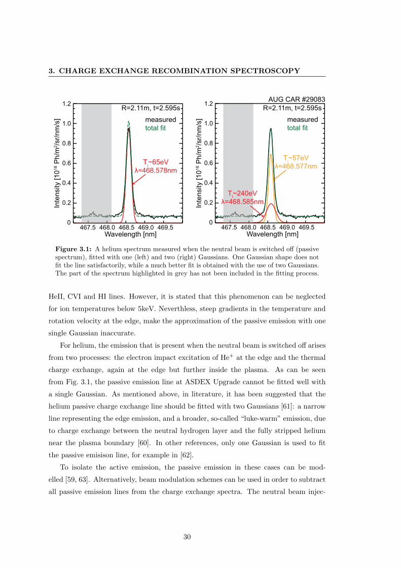
3. CHARGE EXCHANGE RECOMBINATION SPECTROSCOPY
Wavelength [nm]467.5 468.0 468.5 469.0
0.2
0.6
0.4
1.2
0.8
1.0
0
Inte
nsi
ty [1
01
8 P
h/m
2/s
r/n
m/s
] measuredtotal fit
R=2.11m, t=2.595s
469.5
Ti~65eV
λ=468.578nm
Wavelength [nm]
AUG CAR #29083
467.5 468.0 468.5 469.0
0.2
0.6
0.4
1.2
0.8
1.0
0
Inte
nsi
ty [1
01
8 P
h/m
2/s
r/n
m/s
] measuredtotal fit
R=2.11m, t=2.595s
469.5
Ti~57eV
λ=468.577nm
Ti~240eV
λ=468.585nm
Figure 3.1: A helium spectrum measured when the neutral beam is switched o↵ (passivespectrum), fitted with one (left) and two (right) Gaussians. One Gaussian shape does notfit the line satisfactorily, while a much better fit is obtained with the use of two Gaussians.The part of the spectrum highlighted in grey has not been included in the fitting process.
HeII, CVI and HI lines. However, it is stated that this phenomenon can be neglected
for ion temperatures below 5keV. Neverthless, steep gradients in the temperature and
rotation velocity at the edge, make the approximation of the passive emission with one
single Gaussian inaccurate.
For helium, the emission that is present when the neutral beam is switched o↵ arises
from two processes: the electron impact excitation of He+ at the edge and the thermal
charge exchange, again at the edge but further inside the plasma. As can be seen
from Fig. 3.1, the passive emission line at ASDEX Upgrade cannot be fitted well with
a single Gaussian. As mentioned above, in literature, it has been suggested that the
helium passive charge exchange line should be fitted with two Gaussians [61]: a narrow
line representing the edge emission, and a broader, so-called “luke-warm” emission, due
to charge exchange between the neutral hydrogen layer and the fully stripped helium
near the plasma boundary [60]. In other references, only one Gaussian is used to fit
the passive emisison line, for example in [62].
To isolate the active emission, the passive emission in these cases can be mod-
elled [59, 63]. Alternatively, beam modulation schemes can be used in order to subtract
all passive emission lines from the charge exchange spectra. The neutral beam injec-
30

3.1 Components of a charge exchange spectrum
AUG #29083
464 466 468 470
Wavelength [nm]
0.2
0.6
0.4
1.2
0.8
1.0
0
Inte
nsi
ty [1
01
8 P
h/m
2/s
r/n
m/s
]
NBI on (t=4.485s)NBI off (t=4.495s)
R=2.00m
CIII
CIV
HeII
Figure 3.2: Example of a helium spectrum when the neutral beam is on (red), comparedto the spectrum measured directly after the neutral beam is switched o↵ (blue).
tion is modulated and a passive spectrum (neutral beam o↵) is subtracted from the
time-adjacent active spectrum (neutral beam on). Although this method increases the
error bars in the spectrum, the uncertainties associated with the passive emission and
with the fact that it may or may not be approximated with a single Gaussian line are
eliminated. An example of a passive and an active helium charge exchange spectrum
measured at ASDEX Upgrade just before and just after the switching o↵ of the neutral
beam injection is shown in Fig. 3.2.
On ASDEX Upgrade, a forward model was developed to describe the edge emission
and to deconvolute the line-integrated measurements [64]. The local emissions obtained
by the deconvolution of the line-integrated measurements were compared with the ra-
diation simulated by the 1D impurity transport code STRAHL. It was found that both
thermal charge exchange and electron impact excitation contribute to the passive C5+
edge emission, with thermal charge exchange being the dominant e↵ect [63]. Neverthe-
less, the measured passive spectra of C5+ can be fitted well with one single Gaussian,
making it di�cult to separate the two contributions. It should be noted that the mea-
sured passive line is a superposition of several Gaussians, corresponding to di↵erent
rotation velocities and ion temperatures. Regarding the passive line component of
He+, on the other hand, it was shown that thermal CX is not the dominant process
31

3. CHARGE EXCHANGE RECOMBINATION SPECTROSCOPY
and that electron impact excitation should be su�cient to describe the observed line
shape. However, a quantitative evaluation was not possible, as the measured passive
intensity is much smaller than the predicted one, because of the helium recycling in the
scrape-o↵ layer and the diagnostic location in-between two limiters [64].
For the core CXRS diagnostic used in this work the passive helium charge exchange
spectra cannot be fitted satisfactorily with a single Gaussian. Nevertheless, it is not yet
clear whether this is due to the line shape consisting of many Gaussians with di↵erent
rotation velocities and ion temperatures, or two distinct emission components from two
di↵erent plasma layers, as implied in the fit shown on the right hand side of Fig. 3.1.
For this reason, the beam modulation technique has been used for the majority of the
results presented in this work.
32

3.1 Components of a charge exchange spectrum
3.1.3 Bremsstrahlung background
Measured charge exchange spectra are superimposed on an emission background due
to bremsstrahlung radiation Pbremsstrahlung:
dPbremsstrahlung
d�=
32⇡
3
✓e2
4⇡✏0
◆r2⇡
3meTe
1
mc2gffn
2
eZe↵
1
�2
exp
✓� hc
�Te
◆, (3.18)
where gff is the free-free Gaunt factor, which is a weak function of the electron tem-
perature Te and e↵ective charge Ze↵
. As such, the bremsstrahlung level in the charge
exchange spectrum depends on the plasma electron temperature Te and density ne as
well as on the e↵ective charge (impurity content) of the plasma. The bremsstrahlung
contribution to the spectrum is a line-integrated value. The bremsstrahlung level mea-
sured in charge exchange spectra can be used to evaluate Ze↵
, using spectral regions
without line emissions, if the electron temperature and density are known (measured
with diagnostics other than charge exchange spectroscopy) [45].
3.1.4 Contribution from the beam halo
Neutral beam halo is a cloud of deuterium neutrals around the injected neutral beam,
which are produced from charge exchange between the injected beam neutrals and
the thermal plasma deuterium ions. As neutrals, they can spread out of the beam
volume before being reionised. An additional emission from charge exchange between
the impurity ion and the neutral beam halo is present in the spectra. The consequence
of not including the halo in the extraction of He2+ densities from the charge exchange
measurements can be significant. In Fig. 3.3, the predicted charge exchange emission
with beam halo neutrals, contributing to the helium charge exchange measurements,
is illustrated. Assuming a flat He2+ concentration profile of 0.2%, the corresponding
charge exchange intensity with and without the contribution from halo neutrals is
shown. The Monte Carlo based code FIDASIM [65] was been used for the calculation
of beam injected neutrals and halo neutrals.
3.1.5 Plume emission
There are additional complications in the interpretation of the charge exchange data. In
particular, helium charge exchange spectroscopy is hampered by the so-called “helium
33

3. CHARGE EXCHANGE RECOMBINATION SPECTROSCOPY
0.0 0.2 0.4 0.6 0.8 1.0ρ
pol
0
5.0
1.0
1.5
2.0
CX
inte
nsi
ty [
10
16
Ph
/m2/s
r/s)
]
ICX
HeII
with halo
without halo
ne(0)=6.5.1019m-3
Te(0)=3keV
Zeff
=1.56
Figure 3.3: The charge exchange intensity that would be observed for three lines-of-sightof the high etendue spectrometer, assuming a 0.2% flat concentration of He2+ in the plasma,for discharge 29083 at t=2.555s. The beam injected and halo neutrals are calculated withFIDASIM.
plume e↵ect”. The plume emission component, described in detail in Chapter 5, is a
non Gaussian spectral contribution whose intensity is the same order of magnitude as
the active charge exchange emission. The He+ ions produced after the charge exchange
reactions in the neutral beam volume can travel a significant distance along the field
lines, where they can be excited by electron impact excitation before being reionised.
The light emitted as they are de-excited, the helium plume emission, exists in the same
wavelength region and is of comparable magnitude to the active charge exchange signal
in the case of helium, while it is negligible for elements such as carbon and boron. Not
taking the helium plume emission into account leads to inaccurate ion temperature
and rotation profiles and overestimated (by up to a factor of 2) helium density profiles.
The helium plume e↵ect has been studied and a model for its interpretation has been
implemented at ASDEX Upgrade in the course of this thesis. The model is presented in
Chapter 5 and the comparison of the model results with the experimental measurements
is discussed.
3.1.6 Contributions from other impurities
A number of lines originating from charge exchange reactions involving impurities other
than the ones intended to be measured may be present in the spectrum. In the case of
HeII spectra, the carbon (CIII) impurity line triplet passive emission is also measured
34

3.1 Components of a charge exchange spectrum
at wavelengths of 464.742nm, 465.025nm and 465.147nm, with a relative intensity of
5:3:1 and the same ion temperature for all CIII lines [60]. An illustration of an AS-
DEX Upgrade measured spectrum can be seen in Fig. 3.2. Other carbon lines in this
wavelength range include CII at 466.586nm, CIV at 465.830nm.
At ASDEX Upgrade, other impurity lines such as nitrogen and tungsten can appear
in the helium spectra. In machines like JET, which operate with beryllium in the plasma
facing components, beryllium lines are expected in the wavelength range of interest,
namely BeIV n=6-5 at 465.85nm, BeIV n=8-6 at 468.525nm and BeII at 467.34nm,
complicating further the fit of the helium charge exchange spectra [60]. No beryllium
sources, however, exist at ASDEX Upgrade.
3.1.7 Fast ion tail
Not only thermal impurity ions can be diagnosed with charge exchange spectroscopy,
but also impurities of higher energies. If, in addition to the thermal impurity popula-
tion, there is also a population of fast impurity ions, then they will have a much more
broadened emission line, due to their higher temperature. This will then appear as
wings in the charge exchange spectra.
In this way, the fast ions from a neutral beam injected in the plasma can be diag-
nosed. Assuming a deuterium beam injected in a deuterium plasma, fast deuterium
ions capture an electron from the neutral deuterium atoms from the beam and end up
in an excited state. The Balmer-↵ light emitted from the deexcitation of these atoms
can be observed:
D +D+ ! D+ +D⇤. (3.19)
The spectral shift due to the higher velocity of the ions allows for the separation of this
component from the other D↵ emissions.
Fast helium ions can also be measured with charge exchange spectroscopy, for ex-
ample when helium neutral beams are injected in the plasma [60], or the helium ions are
accelerated by ICRH (3He ions). The fast helium ion wing in the charge exchange spec-
tra is also present due to fusion produced ↵-particles. This has been seen in machines
that had D-T operation [66].
35

3. CHARGE EXCHANGE RECOMBINATION SPECTROSCOPY
3.2 Charge exchange recombination spectroscopy as a
plasma diagnostic
3.2.1 Physical quantities from CX spectra
Active charge exchange recombination spectroscopy is a standard diagnostic in many
fusion experiments, as it provides vital information on plasma parameters such as the
ion temperature, plasma rotation and impurity content in the plasma core.
Assuming that the impurity has a Maxwellian velocity distribution, it has been
shown that the observed charge exchange emission line has a Gaussian shape. The
diagnostic capabilities of charge exchange spectroscopy are based on the interpretation
of this line shape in order to provide information on the impurity ion temperature Ti,
the plasma rotation v� and the impurity content ni. These values are extracted from
the measured spectrum as follows (see also Fig. 3.4):
ACX
PCX
Wavelength [nm]
Inte
nsi
ty [
Ph
/m2/s
r/n
m/s
]
Wavelength [nm]
Inte
nsi
ty [
Ph
/m2/s
r/n
m/s
]
λ0
λ
w ~ Ti
Δλ ~ vrot
∫I ~ ni
Δλ
w
∫I
Figure 3.4: An illustration of the active (ACX) and passive (PCX) emissions contributingto a typical charge exchange spectrum (left). The information that can be extracted fromthe active charge exchange emission line is illustrated on the right.
a) The ion temperature Ti causes the Doppler broadening of the line and is as such
related to the width of the measured Gaussian line:
kTi =mc2FWHM2
8 ln 2�2
0
, (3.20)
where k is the Boltzmann constant and FWHM the full-width-half-maximum of the
36

3.2 Charge exchange recombination spectroscopy as aplasma diagnostic
line.
b) The component of the rotation velocity along the line-of-sight causes the wave-
length shift of the Gaussian line. The rotation velocity vrot can therefore be calculated
as:
vrot =��rotc
�0
cos↵, (3.21)
where ↵ is the angle between the line-of-sight and the toroidal direction.
c) The integral over wavelength of the intensity of the emission line is related to the
local impurity density nimp:
nimp =4⇡RI(�)d�
nbQe↵
CX(�b)dl. (3.22)
In practice, charge exchange measurements are made using injected neutral beams
or gas pu↵s. This work has utilised solely charge exchange spectroscopy on a neutral
beam. Using a neutral beam for the neutral source, active charge exchange provides lo-
calised measurements (in contrast to line integrated measurements), as the light emitted
after the charge transfer reaction between the neutral beam atoms and the impurity ion
is coming from the intersection of the observation line-of-sight and the neutral beam.
In Fig. 3.5, the areas from which the active and passive emissions originate are drawn
for one line-of-sight, in a top-down view of ASDEX Upgrade. How accurately localised
the measurement is depends on this path through the beam volume and defines the
radial resolution of the measurement.
In general, charge exchange emission lines with wavelengths in the visible are pre-
ferred for diagnostic purposes, as this simplifies significantly the required optical equip-
ment and instrumentation. Impurities that are routinely observed with charge exchange
spectroscopy include helium, boron, carbon, nitrogen, oxygen and argon.
As already described, the charge exchange spectra are superpositions of active and
passive emission lines on a bremsstrahlung background. Interpreting the spectra means
fitting all the separate contributions in order to extract values with a physical meaning.
Fitting the charge exchange spectra on ASDEX Upgrade is performed using a least
square fitting code, called CXSfit [67], which can deal with the full complexity of
the spectra. The active and passive components of the helium emission as well as
the background level (considered flat within a narrow wavelength range) have to be
identified in the fitting process.
37

3. CHARGE EXCHANGE RECOMBINATION SPECTROSCOPY
0.5 1.0 1.5 2.0 2.5 0
0.5
1.0
1.5
2.0
2.5
NBI
LOS
ACX
PCX
x [m]
y [m
]
PCX
14
15
16
1
Figure 3.5: Top-down view of ASDEX Upgrade, where the locations of active and passivecharge exchange emission are highlighted, for one line-of-sight. The red line represents thepath of Q3, the main ASDEX Upgrade heating beam used for charge exchange measure-ments. The active charge exchange measurement is localised, as the emission comes onlyfrom the intersection of the line-of-sight with the neutral beam. The passive charge ex-change emission originates from the two intersections of the line-of-sight through the coldplasma edge.
3.2.2 Derivation of impurity density profiles
The ability of charge exchange to provide absolute impurity density profiles relies on
information on the neutral beam density in the plasma, see Eq. (3.22). This information
can be obtained either from neutral beam attenuation codes, or from beam emission
spectroscopy (BES), described in detail in section 2.3. Both options are associated with
uncertainties. The errors in the determination of the neutral beam density in the plasma
using BES involves the errors in the measurement and calibration of the instrument, as
well as the atomic rates which determine the emission, while neutral beam attenuation
codes also depend on the quality of the beam stopping rates used and the uncertainties
in the density measurements. The importance of the atomic data in the interpretation
of beam emission spectra is clearly described in [68]. The measurement uncertainties
38

3.2 Charge exchange recombination spectroscopy as aplasma diagnostic
in the electron density and temperature increase the uncertainties. Furthermore, the
beam halo provides an additional complication.
At ASDEX Upgrade, the Monte Carlo forward modelling code FIDASIM [65, 69]
provides the density of neutrals in the beam volume, as well as the beam halo. Also,
beam emission spectroscopic measurements are available that can provide the neutral
beam density.
Combining charge exchange and beam emission spectroscopy data provides a very
useful method to obtain absolute impurity density profiles without the need for an
absolute intensity calibration of the diagnostic. The measured charge exchange and
beam emission intensities are:
ICX /Z
losnimp
X
i=E,E/2,E/3
Qe↵,iCXni
bdl (3.23)
IBES / neQBES
Z
losnibdl, (3.24)
where i represents the di↵erent energy components in the beam. If the same lines-of-
sight are used for the two measurements, then determination of the intersection integral
between the neutral beam and the line-of-sight is not needed. For neutral beam density
equal to nib = f i IBES
QBESne, where f i are the beam energy fractions, then the impurity
concentration is given by [47]:
cimp =nimp
ne= ICX
X
i=E,E/2,E/3
QBES
QCXIBES. (3.25)
Taking into account that the sensitivities of the detectors measuring the charge ex-
change and beam emission spectra are not equal, calibration factors should be included
in Eq. (3.23) and Eq. (3.24), namely ACX and ABES . The ratio of these calibration
factors can be derived by comparing the background bremsstrahlung levels in the two
spectra at the corresponding wavelength, performing a cross-calibration of the two
detectors [70]:ACX
ABES=
CCX
CBES
�CX
�BES, (3.26)
where CCX and CBES are the continuum levels of each of the spectra at wavelengths
�CX and �BES , respectively. Using this method, no absolute calibration of the detectors
is required; all the required information to obtain absolute impurity density profiles
39

3. CHARGE EXCHANGE RECOMBINATION SPECTROSCOPY
can be found in the spectra themselves in order to relatively calibrate the spectra. An
illustration of this technique for the calculation of absolute carbon density profiles in
TEXTOR can be found in the Appendix A.
3.2.3 Charge exchange cross sections and cross section e↵ects
The charge exchange cross-sections, required for the calculation of impurity densities
from the observed charge exchange emissions, depend on the collision energy of the
neutral and the ion. The total cross-sections for charge exchange between fully stripped
helium impurities and hydrogen neutral beams as a function of collision energy are
shown on the left of Fig. 3.6, while the e↵ective charge exchange emission coe�cients
for the HeII n=4-3 transition are shown on the right, for the n=1 and n=2 excited state
of deuterium. The e↵ective cross-sections showcase a maximum at a specific collision
energy (⇠ 30keV/amu in the case of He (n=4-3)), dropping strongly at lower or higher
energies.
The deuterium population in an excited state is much less than the deuterium in
the ground state (⇠ 1%). Nevertheless, as can be seen from Fig. 3.6, the cross-sections
between He2+ and D(n=2) are about two orders of magnitude larger than those for
D(n=1), making their contribution to the charge exchange spectra significant. The
deuterium population in the n=3 excited state is even less than that in the n=2. The
e↵ective emission rates between B5+ and H(n=3) are shown to be of the same order of
magnitude as those between B5+ and H(n=2) and it can be important in high density
conditions [57]. In ASDEX Upgrade plasmas, the contribution from the n=3 excited
state of deuterium is negligible.
For the derivation of Eq. (3.11), it was assumed that Qe↵
CX(�col) ⇡ Qe↵
CX(�b), which
is valid as long as �th ⌧ �b. However, when the temperature and thus thermal velocity
of the ions is large, then a wide range of �col comes into play for the calculation of the
e↵ective emission rate. When a broad Maxwellian distribution function is convolved
with an e↵ective emission rate that varies significantly, a distorted emission line is pro-
duced that deviates from the previously discussed Gaussian line shape. This distortion,
termed cross section e↵ects, depends on the ion temperature, the beam injection energy
and the observation geometry in relation to the neutral beam. Analytical approxima-
tions of the cross section e↵ects are presented in [72] and corrections to the apparent
ion temperatures and velocities are given.
40

3.2 Charge exchange recombination spectroscopy as aplasma diagnostic
0.1 1.0 10.0 100.0
0.1
1.0
10.0
qcx#h0_old#he2qcx#h0_en2_kvi#he2
n=2 [/100]
n=1
He2+ + H(n) → He+ + H+
Ecol
[keV/amu]
σC
X,to
t [10
-20m
2]
0.1 1.0 10.0 100.0
0.1
1.0
10.0 qef93#h_he2qef97#h_en2_kvi#he2
n=2 [/100]
n=1
He2+ + H(n) → He+ + H+
Ecol
[keV/amu]Q
CX
,n=
4-3 [10
-15
m3/s
]e
ff
HeII (n=4-3)
ne=5.1019m-3
Ti=1.5keV
Zeff
=1.56
ADAS:
ADAS:
Figure 3.6: Atomic data for helium charge exchange spectroscopy, obtained fromADAS [71]. On the left, total cross-sections for charge exchange between fully strippedhelium impurities and hydrogen neutral beams. On the right, e↵ective charge exchange co-e�cients for the HeII n=4-3 transition, for typical plasma parameters. The ADAS datasetsfrom which the atomic data come from are annotated.
As an illustration, we use the approximate function presented in [72] for the e↵ective
emission rate of helium, using the observation geometry of the main CXRS diagnostic
on ASDEX Upgrade. We overplot a Maxwellian distribution with an ion temperature
of 3keV, typical of ASDEX Upgrade plasmas, for a neutral beam injection energy
of 30keV/amu. In addition, a Maxwellian distribution of 25keV for a neutral beam
injection energy of 100keV/amu, which will be the energy of the diagnostic neutral
beam on ITER, is plotted as well. As can be seen in Fig. 3.7, in the case of lower
temperatures, a much smaller range of the emission rate is sampled, while in the case
of high temperature, the variation of the emission rate is significant. In general, cross
section e↵ects are negligible for ion temperatures up to a few keV.
In Figure 3.8, the true and observed ion temperature and rotation velocity profiles
are simulated using the approximations discussed in [72]. The simulation corresponds
to the actual observation geometry of the charge exchange diagnostic used in this thesis,
for a 60keV deuterium beam (source Q3 of NBI 1) and charge exchange measurements
on the HeII line at 468.6nm, taking into account only the first energy component
of the beam. The e↵ect on the ion temperature profile is minimal, less than 1%,
41

3. CHARGE EXCHANGE RECOMBINATION SPECTROSCOPY
0 50 100 150 200
Ecol
[keV/amu]
0
1
2
3
4
5C
X e
mis
sio
n r
ate
[1
0-1
5 m
3/s
]
Ma
xwe
llian
velo
city distrib
utio
ns [a
.u.]
Ti = 25 keV
Eb = 100 keV/amu
Ti = 3 keV
Eb = 100 keV/amu
Q(Ecol
)
FWHM
Figure 3.7: The charge exchange emission rate of helium, calculated using the approxima-tion function found in [72], is plotted together with two illustrative Maxwellian distributionfunctions. The dashed line corresponds to a relatively low ion temperature (3keV) and abeam injection energy of 100keV/amu, as the diagnostic neutral beam will be on ITER.The dotted line corresponds to higher ion temperature (25keV). The range of the emissionrate that is sampled by these two velocity distributions is highlighted in green and red,respectively.
while the e↵ect on the rotation velocity profile is somewhat larger, between 2-3%. The
measurement error bars on this diagnostic can be as low as 1.5%, assuming that there is
su�cient signal. The cross-section e↵ects have been, therefore, ignored in the analysis.
3.2.4 Charge exchange spectroscopy for fast ions
Not only thermal ions can be diagnosed with charge exchange spectroscopy, but also ions
of higher energies. If, in addition to the thermal population, there is also a population
of fast ions, then they will have a much more broadened emission line, due to their
higher temperature. This will then appear as wings in the charge exchange spectra.
Fast ions in the plasma undergo charge exchange reactions with neutrals from the
neutral beam. Assuming a deuterium beam injected in a deuterium plasma, fast deu-
terium ions capture an electron from the neutral deuterium atoms from the beam and
end up in an excited state. The Balmer-↵ light emitted from the deexcitation of these
atoms can be observed:
D +D+ ! D+ +D⇤. (3.27)
42

3.2 Charge exchange recombination spectroscopy as aplasma diagnostic
vφ
[km
/s]
(Tru
e-O
bse
rve
d)/
Tru
e [%
]
ρφ
ρφ
trueobserved
trueobserved
vφ
Ti
0.0 0.2 0.4 0.6 0.8 1.00.0
0.5
1.0
1.5
2.0
2.5
3.0
ρφ
0.0 0.2 0.4 0.6 0.8 1.00
20
40
60
80
100
0.0 0.2 0.4 0.6 0.8 1.0-1
0
1
2
3
4T
i [ke
V]
Figure 3.8: True and observed Ti
and vrot
profiles for charge exchange measurements onthe HeII line at 468.6nm. The simulation is based on the analysis performed in [72], fora 60keV deuterium beam, taking into account only the first energy component. The realgeometry of the high etendue spectrometer used in this work, described in 3.3, focused onsource Q3 of NBI 1 is used. On the right, the corrections in the measurement, expressedas the di↵erence between the observed and true value and normalised over the true value,are shown.
The spectral shift due to the higher velocity of the ions allows for the separation of this
component from the other D↵ emissions.
The technique is usually called FIDA (fast ion D-alpha) spectroscopy, despite be-
ing, in principle, an application of charge exchange spectroscopy. FIDA spectroscopic
diagnostics have been implemented among others at DIII-D [73] and ASDEX Upgrade
[74]. An example of a deuterium spectrum, where the FIDA emission is highlighted, is
found in Fig. 3.9.
Dα
CII
BES
2
4
3
0
Inte
nsi
ty [1
01
8 P
h/m
2/s
r/n
m/s
]
1
Wavelength [nm]654 656 658 660652 662
AUG CBR #29510
R=1.77m, t=1.150s
FIDA
Figure 3.9: Example spectrum of deuterium, with the red shifted FIDA emission high-lighted. The D
↵
emission (saturated) as well as the beam emission are also shown.
43

3. CHARGE EXCHANGE RECOMBINATION SPECTROSCOPY
At each wavelength of the FIDA spectrum, fast ions of di↵erent pitch angles and
energies can contribute. The measurement is a one-dimensional projection of the fast
ion distribution in velocity space. A FIDA diagnostic weights the fast ion distribution
function in velocity space, with the weight function being a complicated function of
energy and pitch angle [75]. It is possible, however, to reconstrunct the velocity-space
distribution function, if su�cient data with di↵erent wavelength shifts and observation
views are available [76]. A Monte Carlo forward model has been implemented on DIII-
D [73] and also adjusted for ASDEX Upgrade [74]. The fast ion distribution function
calculated with TRANSP [77, 78] and the computed neutral beam and halo densities
are used to derive the spectral intensity and to compare with the measurements.
Using charge exchange spectroscopy for fast ion measurements is not limited to
deuterium ions. Fast helium ions can also be measured. FIDA spectroscopy allows
for the investigation of subjects such as the fast ion transport and the e↵ect of MHD
instabilities such as sawteeth on fast ions [74], as well as the e↵ect of ion cyclotron
resonance heating on the fast ions [75].
3.3 CXRS diagnostic instrumentation at ASDEX Upgrade
ASDEX Upgrade is equipped with an extensive suite of charge exchange diagnostics,
covering both the core and the edge [63]. An overview of the charge exchange diag-
nostics can be seen in Fig. 3.10. In the course of this thesis work, a high etendue
spectrometer suitable for core charge exchange spectroscopy on ITER has been in-
stalled and utilised on ASDEX Upgrade [79]. With this spectrometer, three separate
wavelength ranges can be observed simultaneously, namely carbon (n=8-7, 529.1nm),
helium (n=4-3, 468.6nm) and D↵(n=3-2, 656.1nm), the last including also the beam
emission spectrum. Details on the spectrometer capabilities can be found in table 3.2,
while an engineering design of the instrument can be seen in Fig. 3.11.
This instrument has been designed according to the ITER requirements for charge
exchange spectroscopy measurements. The core charge exchange diagnostic on ITER
is expected to provide measurements of Ti, �� and helium “ash” concentration. The
ITER charge exchange diagnostic requirements are listed in Table 3.1. However, charge
exchange spectroscopy will face a number of challenges in ITER. The high electron den-
sity of ITER plasmas means high bremsstrahlung background in the charge exchange
44

3.3 CXRS diagnostic instrumentation at ASDEX Upgrade
spectra, and also strong attenuation of the neutral beams. The higher continuum level
makes distinguishing the emission line more di�cult, while the fact that fewer neutrals
from the beam reach the plasma core means much fewer charge exchange reactions and,
therefore, lower signal. Moreover, strong deterioration of the front optics is expected
on ITER, lowering the amount of collected light even further: the first mirror reflectiv-
ity and characteristics are strongly a↵ected by erosion and redeposition due to plasma
ions [80], which will be more severe in ITER than in present devices.
-3 -2 -1 0 1 2
-2
-1
0
1
2
3
14
15
16123
4
5
6
7
8 9 10 11
12
13
1.00 1.50 2.00 2.50
-1.0
-0.5
0.0
0.5
1.0
NBI box 1
#3#4 #1
#2
Optical head
CMRCPR
CHR
NBI box 2
CPR
CMR
CER(HES)
CER(HES)
Figure 3.10: Top down (left) and poloidal cross-section view (right) of ASDEX Upgrade,showing the lines-of-sight and measurement locations of the core and edge charge exchangediagnostics available on ASDEX Upgrade. The high etendue spectrometer (HES) used inthis work employs a subset of the CER lines-of-sight, looking at neutral beam source Q3of NBI box 1, shown in red. The lines-of-sight intersect partially also the other three beamsources of this injector, shown in orange.
The high etendue spectrometer has, accordingly, been designed to deal with the
unfavorable ITER environment. The signal-to-noise ratio of the measurement depends
on the exposure time texp, the spectral resolution ��/� and the detector sensitivity
R [82]:
S
N/rtexp
��
�R. (3.28)
45

3. CHARGE EXCHANGE RECOMBINATION SPECTROSCOPY
Table 3.1: Requirements for core charge exchange spectroscopy measurements per plasmaparameter on ITER [81].
Parameter Location Time Spatial Accuracyresolution resolution
Ti
r/a<0.9 100ms a/10 10%vrot
10ms a/30 30%Ze↵
10-100ms a/10 10-20%Impurity densities r/a<0.9 100ms a/10 20%Core helium r/a<0.9 100ms a/10 10%Confined ↵ Energy <3.5MeV 100ms a/10 20%
The detector sensitivity is defined as:
R = QE · T ·�⌦ ·A, (3.29)
where QE is the quantum e�ciency, T the transmission and �⌦ · A the etendue of
the optical system. For this reason, an optical system with high optical e�ciency,
good spectral resolution and an etendue value of 1mm2sr has been constructed. Mea-
suring simultaneously impurity charge exchange spectra and the beam emission spec-
trum (found in the D↵ spectrum) allows for determination of absolute impurity density
profiles, without the need for absolute intensity calibration of the detectors (see Sec-
tions 3.2.2 and A).
The high light collection capability of the instrument allows for measurements even
with quite low impurity content in the plasma in comparison to other charge exchange
spectrometers. The noise level is also low, and subsequently the error bars on the
spectrum and on the derived profiles are also smaller than in instruments with lower
etendue. The high spectral resolution allows for identification of the di↵erent impurity
lines in the spectra and identification of lower intensity emission lines that might in-
terfere with the interpretation of the emission line of interest. However, on ITER the
expected signal-to-noise ratio is so low (see Chapter 7) that one spectrometer like the
one described here is foreseen for each radial channel in the plasma core, while at the
plasma edge more than one radial location will be measured per spectrometer.
The detectors of the original spectrometer design were three Andor iKon charge-
coupled devices (CCD detectors), one for each spectrometer channel. A chopper was
used so that the camera chips could be kept dark during the readout period. Unfor-
46

3.3 CXRS diagnostic instrumentation at ASDEX Upgrade
Table 3.2: Design parameters of the high etendue spectrometer [79].
Etendue 1mm2srF/# F/1Resolution ⇠ 0.2nmDispersion ⇠ 0.02nm/pxE�ciency 55%(0.92 transmission ⇥0.6 grating e�ciency)Lines-of-sight 54 (400µm) / 27 imaged / 15 on CER periscope
HeII CVI D↵/ BESWavelength 460-474nm 520-534nm 648-667nmGrating order 7th 6th 5th
Figure 3.11: Engineering design of the high etendue spectrometer. The light enters thespectrometer from a single slit and is split with dichroic filters into three wavelength ranges.Each wavelength channel has its own slit. The di↵erent di↵raction orders of a single gratingare used for the di↵erent wavelengths [79].
tunately, the use of the chopper limited the exposure time to approximately 21msec,
with a cycle time of approximately 68ms, meaning a dark time in between acquisitions
of 47ms. For this reason, an upgrade of the detectors was implemented. The helium
channel is now equipped with an Andor iXon EMCCD (Electron-Multiplying Charge-
Coupled Device), while the carbon and D↵ channels are equipped with Andor Neo
sCMOS (scientific Complementary Metal Oxide Semiconductor) detectors. The sC-
MOS detectors were mainly selected because of their ability to deliver short exposure
times, down to the millisecond range. An sCMOS detector is not employed for the he-
lium channel, since the quantum e�ciency of these detectors at the helium wavelength
47

3. CHARGE EXCHANGE RECOMBINATION SPECTROSCOPY
is unacceptably low (46%).
The spectrometer has been operated regularly with an integration time of 10ms on
all channels. However, the helium channel has been operated with shorter integration
times, down to 4ms, and the other two channels with integration times down to 2ms,
depending on the requirements of the experiment. For these short exposure times, the
collected light has been su�cient for measurements, with the exception of carbon, for
which longer integration times were usually required due to the low carbon content in
ASDEX Upgrade plasmas.
The spectrometer detectors are triggered externally from the ASDEX Upgrade trig-
gering system. One second before the discharge is initiated, a number of background
frames are acquired, to be used for the subtraction of the detector background from
the spectra (DVI1 trigger). The series of triggers for acquisition during the discharge is
initiated with the TS06 trigger which signifies the beginning of the plasma discharge.
The acquired raw data are transferred from the detectors’ bu↵ers to local PCs and
from there to the ASDEX Upgrade storage system, where they are stored in the form
of shotfiles (ASDEX Upgrade shotfile system). The raw data shotfiles, called Level 0
shotfiles, contain the measured spectra as well as further information on the acquisition,
for example, the names of the lines-of-sight used, exposure time, spectrometer details
etc.. The Level 0 diagnostic names are CAR, CBR and CCR for the helium, D↵ and
carbon channels, respectively. The analysed data, obtained after fitting the measured
spectra with CXSfit, namely the ion temperature, plasma rotation and intensity profiles,
are stored in Level 1 shotfiles, with diagnostic names CAZ, CBZ and CCZ, respectively.
The calculated impurity densities are stored in Level 2 shotfiles, named CAS, CBS and
CCS, respectively. In this work these names will be used to refer to the data obtained
from these diagnostics.
The spectrometer measures 15 radial locations in the plasma, between the magnetic
axis and the plasma edge, enabling full radial low-field side profiles to be measured,
with a possibility to measure up to 27 radial locations upon request. The lines-of-sight
are focused on beam source Q3 of NBI 1, see Fig. 3.10, but also partially intersect
the other three beam sources (for a more detailed description of the ASDEX Upgrade
neutral beam injection system see section 2.2.1). Further details on the optical head
properties can be found in [63]. The lines-of-sight geometry is obtained by the FARO 3D
48

3.3 CXRS diagnostic instrumentation at ASDEX Upgrade
measurement technology [83], which provides the coordinates of points along the lines-
of-sight. The measurement locations in the plasma, in other words the intersections
between the lines-of-sight and the neutral beams, are then calculated.
3.3.1 Calibration of CXRS measurements
The analysis of charge exchange spectra relies on the calibration of the instrumentation
used. Determination of the measured wavelengths is required for the derivation of the
ion temperature and toroidal rotation, while a conversion of detector counts to collected
photons is required for the derivation of impurity densities.
In order to extract accurate information on the ion temperature and plasma ro-
tation, wavelength calibrations of the spectrometer are required. The wavelength cal-
ibration is performed using laboratory pen lamps of elements that have well-known
emission lines in the wavelength range of interest (for example neon or xenon). In
addition, knowledge of the instrument function is required to allow for deconvolution
of the measured line to extract ion temperature measurements.
580 600 620 640 660pixels
0
0.5
1.0
1.5
2.0
De
tect
or
cou
nts
[1
04] Xe
fitHeII
467.123nm
469.097nm
1460 1500 1540 15802
4
6
8
pixels
De
tect
or
cou
nts
[1
03] Ne
fitCVI
530.476nm
529.819nm
700 800 900 10000
0.5
1.0
1.5
2.0
2.5
3.0
3.5
pixels
De
tect
or
cou
nts
[1
04] Ne
fitD
α
650.653nm
653.288nm
(a) (b) (c)
Figure 3.12: Neon and xenon spectra examples for each channel of the high etenduespectrometer, used for wavelength calibration of the instrument and determination of thedispersion and instrument response function. a) Xenon spectrum in the helium wavelength.The dispersion is 0.0186nm/px (pixel size 13µm) and the � width of the fitted Gaussian lineis 0.029nm. b) Neon spectrum in the carbon wavelength. The dispersion is 0.0118nm/px(pixel size 6µm) and the � width of the fitted Gaussian line is 0.037nm. c) Neon spectrumin the D-alpha wavelength. The dispersion is 0.0135nm/px (pixel size 6µm) and the �width of the fitted Gaussian line is 0.034nm.
The dispersion of each spectrometer channel is determined using two or more well
known emission lines when the spectrometer fibers are illuminated with a neon (for the
carbon and D↵ channels) or a xenon (helium channel) pen lamp. For two emission lines
49

3. CHARGE EXCHANGE RECOMBINATION SPECTROSCOPY
with known wavelengths �1
(nm) and �2
(nm) > �1
and pixel locations px1
and px2
,
respectively, the dispersion d is then identified as follows:
d[nm/px] =�2
� �1
px2
� px1
. (3.30)
Example fitted neon spectra for the calibration of the carbon and D↵ channels and an
example fitted xenon spectrum for the calibration of the helium channel are shown in
Fig. 3.12. A single Gaussian is used to fit the lines.
The shape of the observed spectrum is a convolution of the actual emission line
shape with the instrument function. The entrance slit of the spectrometer has a finite
width which causes the instrumental broadening. Assuming an infinitesimally narrow
emission line, the instrument function is the observed, broadened line shape. The xenon
or neon lines for all spectrometer channels can be fitted well with a single Gaussian.
Finally, each spectrometer channel has its own entrance slit, shown in Fig. 3.11, and
therefore has a di↵erent instrument response function.
462 466 470 474Wavelength [nm]
0
1
2
3
4
De
tect
or
cou
nts
[1
05]
Spectrometer In-vessel
HeII
Ulb
rich
t sp
he
re r
ad
iaa
nce
[W/m
2/n
m/s
r]
0.0
0.1
0.2
0.3
0.4
0.5
500 550 600 650 700Wavelength [nm]
HeII CVI Dα
Figure 3.13: On the left, the spectral radiance curve of the Ulbricht sphere used forthe intensity calibration of the instrument. The wavelength ranges for the three channelsof the high etendue spectrometer are highlighted. On the right, a white light spectrumexample for the helium channel of the high etendue spectrometer, obtained with the Ul-bricht sphere. The solid line represents the measurement when the spectrometer fibers areilluminated with the integrating sphere, while the dashed line corresponds to the in-vesselmeasurements. The ratio of the two curves gives the transmission of the optical path fromthe torus to the spectrometer.
The intensity calibration of the diagnostic is performed by illuminating the spec-
trometer fibers with an integrating Ulbricht sphere whose spectral radiance is known,
see Fig. 3.13. This allows for absolute measurements of the collected light intensity,
as the counts recorded on the detectors can be converted into photons, but also the
50

3.3 CXRS diagnostic instrumentation at ASDEX Upgrade
sensitivity of the detectors across the pixels is identified. The calibration provides the
conversion factor of the counts recorded on the detector to photons, which is calculated
as:
A =R�
ulb[W
m2·sr·nm ]
counts�/texp, (3.31)
where Rulb is the ulbricht sphere radiance at wavelength �, counts is the number of
counts recorded on the detector and texp the exposure time used for the acquisition.
Furthermore, the transmissions of the optics from the in vessel optical compo-
nents to the spectrometer entrance slit have to be characterised. This is achieved by
comparing the measured light when the spectrometer fibers are illuminated with the
integrating sphere to the measurement when the integrating sphere is placed inside the
torus (in-vessel intensity calibration), in front of the diagnostic optical head. Knowing
the transmissions allows for flexibility in the operation, as the spectrometer settings
can be changed independently.
An example white light spectrum for the helium channel is shown in Fig. 3.13. The
solid line represents the measurement when the spectrometer fibers are illuminated with
the integrating sphere, while the dashed line corresponds to the in-vessel measurements.
The ratio of the two curves gives the transmission of the optical path from the torus
to the spectrometer. The wavelength axis is determined using laboratory pen lamps as
described above.
CXRS measurement uncertainties
Uncertainties in the interpretation of the charge exchange measurements arise from the
instrument calibration, but also from the fitting procedure. The radial resolution of
the measurement depends on the diagnostic observation geometry and the intersection
of the lines-of-sight and the neutral beam. The wavelength calibration and character-
isation of the instrument dispersion and instrument function are also characterised by
uncertainties, which are, however, not taken into account in the calculation of the error
bars of the temperature and rotation profiles.
The error bars on the charge exchange spectrum intensity are defined by the photon
noise and the readout noise. Additional uncertainties come into play because of the
detector background subtraction and the smear correction (found to be almost negli-
gible in most cases for the instrument described here). When the beam modulation
51

3. CHARGE EXCHANGE RECOMBINATION SPECTROSCOPY
technique is applied, the error on the spectrum is defined asq
�I2on
+ �I2o↵
, where �Ion
and �Io↵
correspond to the intensity errors of the time frame when the beam is on and
the time frames when the beam is o↵, respectively.
The uncertainties on the impurity density profiles measured with charge exchange
include the uncertainty on the measured intensity and the fitting of the spectra, as
mentioned above. Furthermore, uncertainties in the calculation of the neutral beam
attenuation and the e↵ective charge exchange emission rates contribute to the error bars
of the impurity density profiles. These contributions are estimated in the calculations
of the uncertainties on the final impurity density profiles.
52

4
Impurity transport theory
1.1 Nuclear fusion
1.2 The role of helium in a fusion plasma
1.3 This thesis
Understanding the transport properties of impurities in fusion plasmas is vital for
the operation of ITER and other future fusion devices. Low-Z impurities, such as the
helium “ash”, can cause dilution of the D-T fuel mixture, while high-Z impurities can
cause radiative collapse of the plasma if they accumulate in the plasma core. The
transport of seeding impurities, such as nitrogen, will also have a significant impact
on the plasma operation. This work concentrates on the transport properties of low-Z
impurities and specifically helium in the plasma core.
Neoclassical transport theory, which provides the necessary corrections to the clas-
sical collisional transport, taking into account the toroidal geometry of the plasma, can-
not by itself describe the radial cross-field transport of impurities in a tokamak plasma
and explain the experimentally observed transport. In a large part of the plasma, tur-
bulence provides the major contribution to the radial transport of impurities. This is
the case particularly for low-Z impurities.
In this chapter, the basic theoretical considerations of impurity transport are given,
with the neoclassical and turbulent components described in Sections 4.2 and 4.3,
respectively. Further studies on helium transport, relevant to the confinement, recycling
and pumping of helium, are reported on in Section 4.4.
53

4. IMPURITY TRANSPORT THEORY
4.1 Radial impurity transport
Charged particles gyrating around magnetic field lines can undergo Coulomb collisions
and thus be transferred to other magnetic flux surfaces. This provides a mechanism
by which transport of charged particles can occur perpendicular to the magnetic flux
surfaces.
Macroscopically, the time evolution of the distribution function f↵ of a species ↵
in a multi-species plasma is given by the Vlasov - Fokker-Planck equation (kinetic
equation):
@f↵@t
+�!v ·rf↵ +e↵m↵
(�!E +�!v ⇥�!
B ) · @f↵@�!v = C↵(f↵) + S↵, (4.1)
where C↵ is the Coulomb collision operator and S↵ contains all source and sink terms.
The kinetic equation can be solved perturbatively using an expansion of the distribution
function [84–87].
The moments of the kinetic equation provide the conservation of particle density,
momentum and energy [88]. The equation for particle conservation can be obtained by
the zeroth moment of the kinetic equation for impurities (denoted by subscript I) and
is given in Eq. (4.2):@nI
@t+r · �I = SI , (4.2)
where �I is the impurity flux density, defined as�!�I = �DrnI+
�!�InI , with nI =RfId
3v
being the impurity density and �!�I = (1/nI)R �!v fId
3v being the flow velocity. SI stands
for the sources and losses (sinks) of the impurity due to processes such as ionisation,
recombination, charge exchange, neutral beam injection and fusion in the case of helium
“ash”. D is a tensor that contains the di↵usion coe�cients along and perpendicular to
the magnetic field.
The transport along the magnetic field is much larger than perpendicular to the
field. Thus, the impurity density and temperature are to lowest order constant on a
flux surface. We are mainly interested in the transport between flux surfaces, the so-
called radial transport. When averaging the transport equation Eq. (4.2) over a flux
surface, one obtains the radial impurity transport equation. For a flux surface label r,
which has a simple relation to the volume enclosed by the flux surface V = ⇡r22⇡Raxis,
54

4.2 Neoclassical impurity transport
the radial transport equation has a simple analytical form:
@nI
@t= �1
r
@
@r(r�I) + SI =
= �1
r
@
@rr(D
@nI
@r� �dnI) + SI ,
(4.3)
where D here represents the flux surface averaged radial di↵usion coe�cient and �d the
flux averaged drift velocity. Both neoclassical and anomalous transport contributes to
D and �d and will be described in the following sections. For SI = 0 and @nI@t = 0, the
logarithmic impurity density gradients is obtained as �d/D.
4.2 Neoclassical impurity transport
Classical transport describes the collisional transport in a cylindrical plasma, in the
presence of a homogeneous magnetic field. However, in tokamaks the magnetic field
has a curvature, which introduces additional e↵ects such as the trapping of particles
due to the magnetic field curvature and the rB drift, that are not taken into account
in the classical transport theory. The corrections to the classical transport theory for a
plasma with toroidal geometry are given by the neoclassical transport theory, meaning
that all fluxes in a tokamak plasma are comprised of a classical and a neoclassical part.
The neoclassical part of the fluxes depends on the plasma collisionality ⌫⇤ defined as the
ratio of the collision frequency ⌫ and the particle bounce frequency ⌫b = ✏3/2�th/qR
of a trapped particle, where q = (r/R)(B�/B✓) is the safety factor, r is the minor
radius of the flux surface, R is the major radius of the tokamak and ✏ = r/R is the
inverse aspect ratio of the flux surface. The low collisionality regime (⌫⇤ < 1) is called
the banana-plateau (BP) regime, while the high collisionality regime (⌫⇤ > ✏�3/2) is
called the Pfirsch-Schluter (PS) regime. The neoclassical particle and heat fluxes are
themselves comprised of three components, namely the classical (CL), banana plateau
(BP) and Pfirsch-Schluter (PS) fluxes:
�NCI = �CL
I + �BPI + �PS
I (4.4)
QNCI = QCL
I +QBPI +QPS
I . (4.5)
55
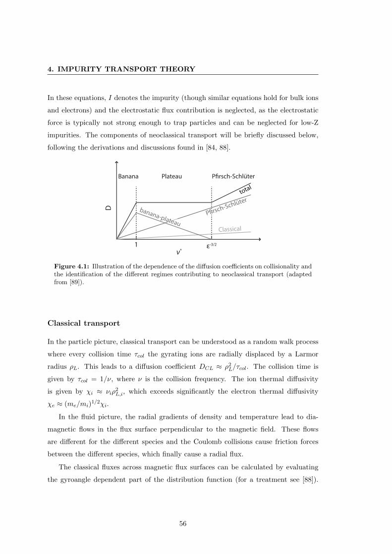
4. IMPURITY TRANSPORT THEORY
In these equations, I denotes the impurity (though similar equations hold for bulk ions
and electrons) and the electrostatic flux contribution is neglected, as the electrostatic
force is typically not strong enough to trap particles and can be neglected for low-Z
impurities. The components of neoclassical transport will be briefly discussed below,
following the derivations and discussions found in [84, 88].
ν*1 ε-3/2
D banana-plateau
P"rsch-S
chlütertot
al
Classical
Banana Plateau P"rsch-Schlüter
Figure 4.1: Illustration of the dependence of the di↵usion coe�cients on collisionality andthe identification of the di↵erent regimes contributing to neoclassical transport (adaptedfrom [89]).
Classical transport
In the particle picture, classical transport can be understood as a random walk process
where every collision time ⌧col the gyrating ions are radially displaced by a Larmor
radius ⇢L. This leads to a di↵usion coe�cient DCL ⇡ ⇢2L/⌧col. The collision time is
given by ⌧col = 1/⌫, where ⌫ is the collision frequency. The ion thermal di↵usivity
is given by �i ⇡ ⌫i⇢2
L,i, which exceeds significantly the electron thermal di↵usivity
�e ⇡ (me/mi)1/2�i.
In the fluid picture, the radial gradients of density and temperature lead to dia-
magnetic flows in the flux surface perpendicular to the magnetic field. These flows
are di↵erent for the di↵erent species and the Coulomb collisions cause friction forces
between the di↵erent species, which finally cause a radial flux.
The classical fluxes across magnetic flux surfaces can be calculated by evaluating
the gyroangle dependent part of the distribution function (for a treatment see [88]).
56
4.2 Neoclassical impurity transport
Classical transport is very small, but there are additional contributions to the particle
transport described by neoclassical theory.
Pfirsch-Schluter contribution
The diamagnetic flows perpendicular to the magnetic field within the flux surface are
not divergence free and parallel flows build up to ensure that the total flow has zero
divergence. These parallel flows are calles the Pfirsch-Schluter flows. Since the diamag-
netic flows of the di↵erent ion species are di↵erent, also the Pfirsch-Schluter flows di↵er.
Here, the Coulomb collisions cause again friction forces between the di↵erent species,
which lead again to a radial flux. This e↵ect causes a di↵usion which is roughly:
DPS ⇡ 2q2DCL, (4.6)
where q is the safety factor. For q values of 3-4, this leads to coe�cients 2q2 = 18� 32
times larger than the classical di↵usion coe�cient.
Banana-plateau contribution
Plasma particles with �k .p✏�? are trapped in magnetic mirrors formed at the outer
side of the torus due to the 1/R dependence of the magnetic field. The particles bounce
between two mirror reflection points and perform so-called banana orbits. Trapped ions
travel along the banana orbit such that they move in the direction of the electric current,
when they are on the outside and against the current on the inside of the banana orbit.
Thus, a similar e↵ect is obtained for the diamagnetic flow due to the gyromotion of the
ions: radial density and temperature gradients lead to a parallel flow of the trapped
particles. These flows cause again a radial flow due to the parallel friction forces. The
resulting di↵usion coe�cient is roughly:
DBP ⇡ q2
✏3/2DCL. (4.7)
However, if the collisionality is above 1, the particles cannot finish their travel along
the banana orbit without undergoing a collision. Thus, the above mentioned anisotropy
of the velocity distribution vanishes for large collisionalities. The corresponding dif-
fusion coe�cient goes to zero for collisionalities much larger than 1. Typically, the
57

4. IMPURITY TRANSPORT THEORY
banana-plateau contribution is negligible when reaching the Pfirsch-Schluter collision-
ality regime.
Low-Z impurities such as helium and boron in the core of a typical ASDEX Upgrade
plasma are typically in the banana-plateau (or long mean free path) regime. The edge
of the plasma is mostly in the Pfirsch-Schluter regime. The transport in the region in
between is characterised by both banana-plateau and Pfirsch-Schluter contributions.
The classical contribution is small in all plasma regions.
4.2.1 Neoclassical predictions of impurity transport
Despite the fact that neoclassical transport theory alone cannot fully describe the im-
purity transport in the plasma, there are plasma regions and plasma regimes in which
neoclassical transport is su�cient to explain the observed transport.
The neoclassical di↵usion coe�cients and drift velocities are the sum of the di↵usion
coe�cients and drift velocities in each of the regimes. The coe�cients can either be
calculated by numerical codes, such as NEOART [89, 90], or with simpler analytical
expressions such as those given in [91]. Total di↵usion and drift coe�cients can also
be derived from experimental measurements, but they would also contain turbulent
contributions. The di↵usion coe�cients for a large aspect ratio circular plasma are
given below [91]:
DNC = DCL +DPS +DBP
DCL =1
B2
0
mIkT⌫IDe2Z2
DPS =2q2
B0
KPSmIkT⌫IDe2Z2
DBP =q2
✏3/2B2
0
kTµ⇤ID
e2ZnI
(4.8)
where k is the Boltzmann constant, q is the safety factor, ⌫ID is the collision frequency
between the impurity and the main ions, B0
is the vacuum toroidal field, KPS is
a function of the impurity strength parameter nIZI2/nD [91, 92] and the main ion
collisionality, µ⇤I is the weighted viscosity coe�cient of the impurity and main ions,
dependent also on ⌫ID, and ✏ the inverse aspect ratio. Here, we just consider the
collisions between the impurity and the main ion deuterium. The collision frequency is
⌫ID / Z2/T 3/2 and DCL is nearly independent of Z. In the plasma core, the banana
58

4.2 Neoclassical impurity transport
plateau contribution dominates the di↵usion, while the Pfirsch-Schluter contribution
dominates the plasma edge.
The convective part of the impurity transport is defined by the drift velocities. The
total neoclassical drift velocity is the sum of the drift coe�cients in each of the regimes.
The drift velocity in each regime is driven by the gradients in deuterium density and
ion temperature:
�NC = �CL + �PS + �BP
�X = DXZ
✓d lnnD
dr+ ↵T
d lnTi
dr
◆(4.9)
where X denotes each contribution (CL, PS, or BP) and ↵T is a function of the impu-
rity strength parameter and the main ion collisionality [91, 92]. The drift velocity is,
therefore, comprised of an inward part, proportional to the main ion density gradient,
and an outward part, proportional to the temperature gradient, as ↵T is negative [93].
This outward contribution to the drift velocity plays a screening role and is described
below.
Temperature screening
Neoclassical transport theory predicts the phenomenon of impurity “temperature screen-
ing”, which leads to impurity transport in the outward direction. The drift velocity of
an impurity can be analytically written as [94]:
�I = DIZ
✓↵n
d lnnD
dr+ ↵Ti
d lnTi
dr+ ↵Te
d lnTe
dr
◆, (4.10)
where the dependence on the gradients is defined by the factors ↵n,↵Ti , ↵Te , which are
functions of the impurity strength parameter and the impurity and main ion collision-
ality. The factor ↵n includes only collisions between the main ions and the impurity,
as momentum transfer between electrons and impurities can be considered negligible,
and for the same reason, ↵Te is very small. If |↵n| � |↵Ti |, impurities are predicted to
have a peaked density profile when the electron density profile is peaked. If, however,
the main ion density profile gradient becomes small then the ion temperature gradient
term becomes important. In the banana-plateau regime the coe�cient of the ion tem-
perature gradient term is negative. This outward convective flux is called temperature
59

4. IMPURITY TRANSPORT THEORY
screening. The temperature screening factor is a complicated function of Z, m and nI ;
no direct conclusions can be drawn for the dependencies of the temperature screening
e↵ect. It is noted in [93] that helium has a higher (but still negative) temperature
screening factor than heavier, higher-Z impurities, and for this reason temperature
screening is expected to be weaker for helium.
Ware pinch
The Ware-pinch [95] is a radial particle flux driven by the toroidal electric field. Due
to the toroidal electric field, trapped particles in banana orbits are accelerated in one
direction, which leads to reduction of their pitch angle, and decelerated in the other
direction, which leads to an increase of their pitch angle. Therefore, the banana orbits
are displaced and a net inward flux is observed. The banana orbits drift towards the
magnetic axis with a velocity of cE�/B✓, where E� and B✓ are the toroidal electric field
and the poloidal magnetic field, respectively. This neoclassical inward flux leads to a
peaking of the density profiles. This e↵ect reduces with collisionality as the banana-
plateau transport and is only important in the hotter central part of the plasma. For
impurities, the Ware pinch is usually small compared to the gradient driven fluxes.
4.2.2 Neoclassical impurity transport observations
Neoclassical transport and the comparison of the neoclassical theory with experimen-
tally derived transport coe�cients has been the subject of research in many tokamaks
over the last decades. In this section, experimental investigations in comparison to
neoclassical theory are briefly reviewed.
In the plasma core (⇢pol < 0.3), di↵usion coe�cients and drift velocities derived from
neoclassical theory compare well with experimental measurements for low-Z impurities
performed at ASDEX Upgrade, with significant discrepancies for higher Z [91]. The
di↵usion coe�cient is stated to be either neoclassical or anomalous inside r ⇠ ↵/4,
with ↵ being the minor radius, with the di↵usion coe�cient increasing strongly and
becoming anomalous when central ECR heating is applied [25]. A strong inward drift is
observed in this region when the di↵usion coe�cient is neoclassical, decreasing strongly
in the anomalous cases. Neoclassical simulations of the di↵usion and drift coe�cients
have shown agreement with the experimental observations in this region for lower-Z
elements. However, they underpredict the coe�cients for high-Z elements [91]. It should
60

4.2 Neoclassical impurity transport
be noted, however, that many past analyses of neoclassical transport were neglecting
the enhancement of neoclassical transport produced by rotation e↵ects, which could be
more than one order of magnitude for heavy impurities.
In the confinement region, defined as 0.3 < r/a < 0.8, the experimentally deduced
di↵usion coe�cients are one order of magnitude larger than those predicted by neo-
classical theory. ASDEX Upgrade and JET results show that the di↵usion coe�cients
are much larger than the neoclassical predicted values, with �/D values smaller than
the neoclassical ones [25, 96]. The impurity transport is anomalous in this plasma re-
gion [25, 27, 97]. Nevertheless, neoclassical transport can become important for higher-
Z elements and at higher collisionalities. This is the region of concern for this work.
In the edge transport barrier region, in H-mode plasmas, impurity transport is ob-
served to be neoclassical and characterised mainly by the Pfirsch-Schluter neoclassical
term [90, 98].
The di↵usion coe�cients deduced from neoclassical theory are in the range of
10�3m2/s to 10�1m2/s, while experimentally deduced coe�cients, which include
anomalous transport due to turbulence, diverge strongly from the neoclassical val-
ues [92]. Strong variations and di↵erent divergences from the neoclassical theory are
found in di↵erent machines due to di↵erent operational regimes and experimental un-
certainties. Nevertheless, the general observation in all tokamak experiments is that
neoclassical transport alone cannot explain the observed impurity density profiles. Neo-
classical transport predicts profiles that are much more peaked than those experimen-
tally measured. As such, both neoclassical and anomalous e↵ects must be considered.
Also in the case of helium, experimental evidence has supported the argument that
there are contributions additional to the neoclassical transport. Helium di↵usivities and
heat conductivities in TFTR supershots were found to be radially hollow, increasing
strongly from the sawtooth inversion radius to the plasma edge and larger by at least an
order of magnitude than those predicted by neoclassical theory, even inside the sawtooth
inversion radius, except for the region around the magnetic axis. Inward convection was
observed to be larger than the neoclassical values for r/a < 0.5 [99, 100]. Furthermore,
evidence for electrostatic turbulence as the dominant transport mechanism has been
identified, as it was observed that DHe(r) ⇠ �i(r) ⇠ ��(r) ⇠ �e(r), as expected
if helium is a trace impurity and the dominant transport mechanism is electrostatic
turbulence.
61

4. IMPURITY TRANSPORT THEORY
In enhanced reversed magnetic shear plasmas in TFTR, the helium di↵usivities
compare well with neoclassical predictions derived with NCLASS [101], within the
reverse shear region (r/a < 0.35) where plasma fluctuations are very small. However,
strong enhancement of the di↵usion coe�cients is observed outside [102, 103], implying
turbulent contributions.
At DIII-D, in plasmas with suppressed turbulent transport, small ion density gradi-
ent, and strong ion temperature gradient (very high confinement mode plasmas [104]),
the so-called “temperature screening” of impurities, which leads to outward impurity
transport, was experimentally documented [94]. In the early phases of these plasmas,
while still in L-mode with strong turbulence, the low-Z impurity density profiles are
observed to have similar shapes compared with the electron density, independent of the
charge and mass of the impurity. In the very high confinement mode phase, the ob-
served transport is found to be enhanced in comparison to the neoclassical predictions,
which is attributed to anomalous transport.
Previous helium studies performed at ASDEX Upgrade also support the evidence
of anomalous helium transport in the confinement region. Di↵usion coe�cients in the
range of 0.4 - 3m2/s and drift velocities of �15 - 0m/s increasing radially from the
core to the edge, are reported for helium and neon, 5-10 times larger the collisional
expectations [105].
As a general conclusion, experimental evidence for helium transport in the confine-
ment region shows deviations from the neoclassical theory predictions. The contribution
of anomalous electrostatic turbulence to the helium transport is significant, if not the
dominant mechanism, and necessary to explain the observed impurity transport.
4.3 Turbulent transport
Neoclassical transport theory cannot explain all of the experimental observations of
impurity transport, meaning turbulence can play an important role in determining
the transport of electrons, impurities and main ions. Depending on the turbulent
plasma state, typically either the Trapped Electron Mode (TEM) regime, in which
trapped electron modes dominate, or the Ion Temperature Gradient (ITG) regime, in
which ion temperature gradient modes dominate, di↵erent behaviours are predicted.
62

4.3 Turbulent transport
constant n
xz
y
B
E
E x B!ow
dri
ft
wav
e
n
more denseless dense
Figure 4.2: Illustration of the electron drift wave.
A complete understanding of impurity transport requires taking both the neoclassical
and the turbulence-induced transport mechanisms into account.
4.3.1 Plasma turbulent states
Plasma turbulence is created by microinstabilities in the plasma, both mainly electro-
static and electromagnetic in nature. For impurities, instabilities of high k, in other
words with short wavelengths comparable to the ion Larmor radius scale, and of mainly
electrostatic nature are of interest. In particular, the TEM instability, driven by the
electron drift wave, and the ITG instability, driven by the ion acoustic wave, are the
dominant players under most conditions.
Electron drift wave
The electron drift wave is a plasma wave of electrostatic nature, responsible for the
development of the trapped electron mode instability [10]. Assuming a slab of plasma
in a shearless, uniform magnetic field in the z-direction, that exhibits a density gradient
in the x-direction, the wave defines density isobars, as shown in Fig. 4.2. The density
perturbation en in the y-direction is of the form n1
= exp i(kyy � !t).
63

4. IMPURITY TRANSPORT THEORY
If the perturbation n1
is identical in phase and magnitude along the magnetic field
(z-direction), then the density along this direction changes as a function of time !t,
but as there is no gradient along the magnetic field direction, there is no instability.
We now assume that n1
has a gradient or phase change in the z-direction. The elec-
trons are adiabatic and flow freely along the magnetic field line, keeping the Boltzmann
relation. In this way, a potential fluctuation �1
is created in the y-direction, given by:
n = n0
+ n1
= n0
exp
✓e�
Te
◆. (4.11)
Linearising the above equation yields:
n1
n0
=e�
Te. (4.12)
There is no phase di↵erence between the density and potential perturbation. As now
the high density regions become positively charged, due to the flow of the electrons,
and the low density regions become negatively charged, an electric field is created by
the potential perturbation in the y-direction:
�!E
1
= ��!r�. (4.13)
The electric field is 90o out of phase with the density perturbation n1
and causes an�!E ⇥�!
B drift in the direction of the density gradient (x-direction):
v�!E⇥�!
B=
�!E
1
⇥�!B
B2
. (4.14)
The radial transport caused by a density perturbation en and a ev�!E⇥�!
Bdrift velocity
is given by �r = hen ·ev�!E⇥�!
Bi sin(�). Since the density perturbation and the drift velocity
are 90o out of phase, sin(�) = 0 and no radial transport is observed.
The continuity equation can now be written:
✓@
@t+ v�!
E⇥�!B·r◆n+ nrv�!
E⇥�!B
= 0. (4.15)
The unperturbed part of the density n0
is constant: @n@t = 0. Moreover, as the
�!E ⇥�!
B
64

4.3 Turbulent transport
flow is along the x-direction, nrv�!E⇥�!
B= n @
@x |v�!E⇥�!B|x = 0. Therefore:
@n1
@t+ v�!
E⇥�!B·rn
0
+ v�!E⇥�!
B·rn
1
= 0. (4.16)
The last term on the left hand side is zero and as such:
@n1
@t= �v�!
E⇥�!B·rn
0
. (4.17)
The time derivative of the density perturbation is:
n1
= exp i(kyy � !t) ) dn1
dt= �i!n
1
. (4.18)
Taking into account that the potential perturbation is in phase with n1
( Eq. (4.12)),
the electric field created is�!E = �r�
1
= �iky�1
. Replacing now in the continuity
equation, the wave frequency obtained:
! = �kyTe
eB
rn0
n0
, (4.19)
which is ky times the electron diamagnetic velocity, assuming no or small temperature
variation.
If a mechanism, such as collisions, Landau damping or a temperature gradient,
make the density perturbation out of phase with the potential perturbation, then ra-
dial transport becomes possible. This can be expressed as a small correction to the
Boltzmann relation (i�-model):
n1
n0
=e�
Te(1� i�). (4.20)
As such, the drift wave is destabilised and leads to turbulent microinstabilities. The
result is turbulent transport due to the so-called electron drift mode microinstabil-
ity [106, 107].
Trapped Electron Mode (TEM)
Trapped particle modes [108, 109] can be categorised into collisionless and dissipative.
In collisionless modes, the trapped particles stay in the bad curvature region for most of
the time, so that the curvature drift is always in the same direction. The�!E ⇥�!
B flows
65

4. IMPURITY TRANSPORT THEORY
can therefore enhance the perturbation. If the collisions, however, become frequent
enough in comparison to the drift frequency, the trapped particles can become passing
and vice versa.
Trapped electron collisions in combination with an electron temperature gradient
provide a destabilising mechanism for the electron drift wave mode, with a growth rate
that depends on the drift wave frequency and the trapped particle velocity dependent
collision frequency, as well as on the ⌘e parameter:
⌘e =1
Te
dTe
dr
✓1
n
dn
dr
◆�1
, (4.21)
where r is the radial coordinate, and dTe/dr is the electron temperature gradient, acting
as the main drive for the instability.
Ion temperature gradient (ITG)
If the ion density perturbation is out of phase with the potential perturbation due to
dynamics acting on the ions, such as the presence of an ion temperature gradient, then
ion drift wave instabilities, such as the ion temperature gradient mode, can occur.
The ion temperature gradient mode can be separated into two structures depend-
ing on whether toroidal e↵ects are responsible. The first one, the ‘slab’ mode struc-
ture [110], evolves from the coupling between a poloidally propagating drift wave arising
due to an ion temperature gradient and a parallel ion acoustic (sound) wave. The par-
allel sound wave compression (z-direction in Fig. 4.2) a↵ects the ion density response,
causing an instability. The toroidal mode structure [111] evolves from the coupling
between the magnetic curvature and the drift wave in the presence of an ion temper-
ature gradient. In this case, the ion density response is changed by the toroidal drift.
The growth rate of the ITG mode depends on the ⌘i parameter, defined as for the
electrons in Eq. (4.21), making clear the dependence of the mode appearance on the
ion temperature gradient.
4.3.2 Turbulent impurity fluxes
Impurity transport caused by electrostatic plasma turbulence, which is non-linear in
nature, can be studied within a fluid or a gyrokinetic approach with a variety of non-
66

4.3 Turbulent transport
linear and quasi-linear models. The dependences of the turbulent impurity fluxes are
analysed in detail in [112–115].
The impurity particle and heat fluxes due to turbulent transport processes can be
decomposed into a di↵usive, a thermodi↵usive, a rotodi↵usive and a convective term
as follows:R�InI
= Dd,IR
LnI
+Dth,IR
LTI
+Du,Iu0I +RVp,I (4.22)
RQI
nITI= �d,I
R
LnI
+ �th,IR
LTI
+ �u,Iu0I +RHp,I . (4.23)
There, the local normalised logarithmic gradients R/LX are defined as:
R
LX= �R
X
dX
dr(4.24)
with r being the flux surface averaged plasma minor radius and R the plasma major
radius, while the radial gradient of the toroidal plasma velocity is given by u0
u0I = �d⌦I
dr
R2
�th, (4.25)
where ⌦I is the angular toroidal rotation velocity.
The decompositions of the turbulent fluxes are comprised of the following contri-
butions:
• The diagonal di↵usive flux is proportional to the local impurity density gradient
and is characterised by the particle di↵usion coe�cient Dd,I in the case of the
particle flux and by the heat di↵usivity coe�cient �d,I in the case of the heat
flux. Di↵usion arises mainly from the�!E ⇥�!
B advection and is, therefore, charge
independent.
• The thermodi↵usion piece is proportional to R/LTi , characterised by the parti-
cle thermodi↵usivity coe�cient Dth,I and the heat conductivity coe�cient �th,I .
Thermodi↵usion arises from the coupling between temperature and density fluctu-
ations, due to the curvature and rB drifts. Due to the inverse charge dependence
of these drifts, the thermodi↵usive contribution to the fluxes is expected to be
more important for lower-Z impurities. Thermodi↵usion is directed inwards when
a TEM is dominant, or outwards when ITG are dominant.
67

4. IMPURITY TRANSPORT THEORY
• The rotodi↵usion part is proportional to the radial gradient of the plasma toroidal
velocity and is characterised by the particle rotodi↵usion coe�cient Du,I and the
corresponding heat coe�cient �u,I . This term arises from the�!E ⇥�!
B advection
in the presence of a background rotation gradient [11]. Similar to the thermodif-
fusion term, the direction of the rotodi↵usion is inward when a TEM is dominant
and outward when an ITG is dominant. Rotodi↵usion is connected with parallel
dynamics and scales with A/Z [115].
• The pure convective part is characterised by the (heat) pure convective velocity.
This pure convection is the result of many mechanisms: the compression of the�!E ⇥ �!
B drift, which provides a charge-independent contribution, the curvature
and rB drifts, which provide a decreasing contribution with increasing charge,
as well as parallel dynamics which is dependent on Z/A. Pure convection is direct
inwards for monotonic q profiles (for the toroidal part). However, the part due
to the parallel dynamics can be directed either outward or inward, depending on
the mode [113, 116].
The coe�cients encountered in each turbulent flux term depend on the mass and
charge of the impurity, as well as on the background main ion plasma properties. A
formulation of the coe�cients can be found in [115] and the references therein.
Both turbulent and neoclassical transport mechanisms should be taken into account
to express the impurity density. Therefore, the local normalised logarithmic impurity
density gradient is given by the ratio of the total convection to the total di↵usion,
taking into account both turbulent (turb) and neoclassical (NC) transport, assuming
that the total impurity particle flux is zero:
R
LnI
= �RV turbI +RV NC
I
Dturbd,I +DNC
d,I
(4.26)
Despite their names, the last three terms of Eq. (4.22) together, namely the thermodi↵u-
sion, the rotodi↵usion and the pure convection, give the total turbulent convection [27].
Assuming only turbulent transport contributions, as is expected in the confinement
region of the plasma and especially around the mid-radius for low-Z impurities, the
68

4.3 Turbulent transport
impurity density logarithmic gradient can be derived from Eq. (4.22), setting �I = 0:
R
LnI
����turb
' �✓Dth,I
Dd,I
R
LTI
+Du,I
Dd,Iu0I +
RVp,I
Dd,I
◆
= �✓CT
R
LTI
+ CUu0I + CP
◆ (4.27)
which can be compared to the one calculated assuming only a neoclassical contribution:
R
LnZ
����NC
= �RV NC
p,I
DNCd,I
. (4.28)
4.3.3 Applications of turbulent transport theory
Though the description here is focussed on impurity transport, turbulent electron trans-
port has provided very important insights on subjects such as the electron density
peaking. The experimentally observed electron density peaking with the application of
central electron cyclotron heating is associated with the transition between the di↵erent
plasma turbulent states (ITG/TEM). An overview of this process is given here, as it is
important for the understanding of the helium transport experimental investigations.
Subsequently, previous work on the turbulent transport of low-Z impurities such as
boron will be presented.
E↵ect of electron heating on the electron density profile
The application of central electron heating has been observed to have di↵erent e↵ects
on the electron density profiles under di↵erent conditions. A flattening of the electron
density profile, also called “pump-out”, has been observed in low density L-mode plas-
mas, but also in high densities, where it was partially attributed to the reduction of the
Ware pinch [26, 95]. On the other hand, under certain conditions, the electron heating
leads to peaking of the electron density profile [26, 27].
Through modelling of the turbulent transport, it has been shown that this behaviour
can be explained by the turbulent plasma state. It was found that there is a clear non-
monotonic relation between the peaking of the electron density with the real frequency
of the most unstable mode !r [26, 27]. Looking at an illustration of the logarithmic
normalised electron density gradient as a function of !r, and as a proxy with the
e↵ective collisionality, shown in Fig. 4.3, the observed behavior of the electron density
69

4. IMPURITY TRANSPORT THEORY
TEM ITG
R/Lne
ωr (ve")1 2 3
Figure 4.3: Illustration of the predicted dependence of the normalised logarithmic elec-tron density gradient on the real frequency of the most unstable turbulent mode !
r
andcollisionality v
eff
in the ITG and TEM regimes.
profile under electron cyclotron heating can be explained. The description below is
according to the present theoretical interpretation of the observations, which is in the
process of being validated.
Starting from very low densities (case 1 in the figure), application of central ECRH
increases the electron temperature and decreases the e↵ective collisionality, leading to
flattening of the electron density. Adding ECRH to an ITG dominated regime (case
2), decreases the e↵ective collisionality leading to a transition from an ITG dominated
towards a TEM dominated regime and peaking of the electron density profile. As this
happens, the thermodi↵usive term contributing to the electron turbulent flux reverses,
from inward to outward and can lead to flattening of the density profile. Considering
now cases with high e↵ective collisionality (case 3), the application of central ECRH
might not be su�cient to change the Te/Ti ratio and hence no change in !r or to the
density gradient is expected. The strongest peaking of the electron density profile is
predicted near the transition from the ITG to the TEM regime, in the TEM regime.
In low density, low current H-mode ASDEX Upgrade plasmas, the electron density
is observed to peak strongly with increasing central electron heating and this behaviour
is again linked to the transition from an ITG to a TEM regime [27]. Good agreement
has been found comparing the measured electron density profiles with the results of
the gyrokinetic simulations.
70

4.3 Turbulent transport
E↵ect of electron heating on the density profile of light impurities
A similar e↵ect of the electron heating via the change in turbulence regimes has been
observed in ASDEX Upgrade also for light impurities, such as boron [11, 27]. Flat and
even hollow boron profiles have been observed in NBI only heated discharges, while the
boron density profiles peak as the dominant turbulent mode transitions from ITG to
TEM. The boron profiles are always observed to be less peaked than the electron den-
sity. Neoclassical transport was found to be negligible in comparison to the turbulent
transport at mid-radius of the plasma.
The gyrokinetic simulations of the logarithmic normalised boron density gradients
compare well qualitatively with the measured profiles, if the rotodi↵usive term is in-
cluded in the simulations [11]. The e↵ect of the background toroidal plasma rotation
profile contributes to the explanation of the peaked boron profiles. Furthermore, the
rotodi↵usive term provides an outward contribution to the flux in the case of peaked
rotation profiles. The rotodi↵usion contribution is almost negligible during phases of
strong electron heating, as the rotation profile flattens in this case. Nevertheless, the
modelling of turbulent transport even including this term cannot fully reproduce the
hollow boron profiles in NBI only phases, indicating that an additional contribution
might be missing from the modelling.
Taking the ratio of electron to ion temperature Te/Ti as a proxy for the collisionality,
it was observed that the thermodi↵usion contribution reverses from outward to inward
in as Te/Ti increases and the transition from ITG to TEM occurs [27]. The same is
observed for the rotodi↵usion term, while pure convection is always directed inwards.
Via the modelling, clear correlations have been found between these o↵-diagonal con-
tributions to the turbulent boron transport and the real frequency of the most unstable
mode.
Since some of the terms contributing to the turbulent particle flux depend on the
impurity charge, variations are expected in the profiles of di↵erent impurities. Com-
paring helium, which is of interest in this work, with the heavier boron, the main
di↵erence is expected to be the thermodi↵usion, which is inversely proportional to Z.
Gyrokinetic modelling of the helium “ash” transport in ITER, including neoclassical
transport (important within r/↵ < 0.1) predicts inward directed convection, but the
71

4. IMPURITY TRANSPORT THEORY
di↵usion is expected to be large enough to avoid helium “ash” accumulation in the core
of the ITER plasma [114].
Motivated by these results and the need to have experimental verification of the
theoretical predictions, in Chapter 6, helium density profiles will be compared with the
boron and electron density profiles as a function of theoretically relevant parameters,
such as the normalized gradients of the electron density, the ion temperature and the
toroidal rotation.
4.4 Experimental studies on helium confinement, exhaust
and recycling
Over the years there has been great interest to identify the properties of the transport
of thermal helium (helium “ash”), with the ultimate goal being to identify a mechanism
that removes the thermalised helium from the plasma, preferably without simultaneous
removal of the high energy ↵ particles. Helium confinement and helium exhaust are
important issues of helium transport that will play a significant role in the operation
of future fusion devices such as ITER.
During the D-T operation of TFTR, helium “ash” was found to transport rapidly
from the center, where it is produced, to the plasma edge, where it is pumped [62].
Using previously calculated values for the di↵usivity and convective velocity [100], the
helium global confinement time ⌧⇤He was calculated to be on the order of 6 � 10 ⌧E ,
where ⌧E is the energy confinement time and, therefore, in the range of what is required
for continuous reactor operation, namely 7 � 15 ⌧E [5]. ⌧⇤He is the mean dwell time of
helium in the vessel and includes the e↵ect of helium recycling and pumping. On the
other hand, ⌧He, without taking recycling into account, was estimated to be on the
order of only two times the energy confinement time. This shows that reflux from the
edge will be the limiting factor determining the removal of helium “ash” and not core
transport.
In TEXTOR, Hillis et al [117] studied the transport and exhaust of helium in L-
mode and in an H-mode-like regime, induced by a polarising electrode. The ALT-II
toroidal belt pump limiter could completely remove the helium from the plasma, and
also provided measurements of He and D↵ in the limiter duct, enabling exhaust studies
to be performed. Helium was pu↵ed into the plasma to simulate the helium “ash”
72

4.4 Experimental studies on helium confinement, exhaust and recycling
and observed with charge exchange spectroscopy at two radial locations. In L-mode
discharges, the pu↵ed helium appears quickly in the plasma core and is then transported
radially to the plasma boundary, where it was seen to be removed by the ALT-II pump
limiter system within 1s. In the enhanced confinement discharges, however, the helium
ions stay in the plasma core for much longer, two or three times longer compared to
the L-mode. The ratios of global particle confinement over energy confinement time,
⌧⇤He/⌧E , was between 9 and 20 in L-mode plasmas, while it increased to ⇠70 in the H-
mode-like plasmas. These high values would be detrimental in future reactor operation.
In connected helium transport studies in DIII-D, the helium recycling coe�cient was
1 in ELM-free phases of H-mode discharges, as the helium density was observed to
be constant. Giant ELMs were observed to expel helium ions from the plasma edge,
leaving the core (⇢ < 0.5) una↵ected.
Helium exhaust studies in improved core confinement or internal transport barriers
scenarios at ASDEX Upgrade with the LYRA divertor, showed that helium exhaust is
low and does not seem to be limited by the core plasma transport [118]. Short helium
gas pu↵s cause a simultaneous and equal increase of the helium density both inside and
outside the transport barrier, which decays rather slowly with the same rate for both
locations.
Finally, helium recycling provides an additional source of helium in the plasma,
increasing the e↵ective helium particle confinement time, as the recycling coe�cient R
(typically close to 1), enhances the particle confinement time by a factor of 1/(1�R).
Understanding helium recycling in current and future machines is also of fundamental
importance, as it relates with the capability to remove the helium “ash” from the
plasma [119].
In summary, the e↵ective particle confinement time has been found both optimistic
(TFTR) and detrimental (TEXTOR H-mode-like operation) for future reactor opera-
tion. In all cases, however, recycling and reflux from the plasma edge are recognised
as the critical factor for the removal of helium “ash”. Even if the transport in the core
is satisfactorily manipulated, this remains a decisive parameter. However, it remains
outside the scope of this work.
73

4. IMPURITY TRANSPORT THEORY
74

5
The helium plume e↵ect
2.1 Tokamak operation
2.1.1 Plasma equilibrium and shape
2.1.2 Magnetohydrodynamic (in)stability
2.1.3 Tokamak wall
2.1.4 The ASDEX Upgrade tokamak
2.2 Plasma heating systems on ASDEX Upgrade
2.2.1 Neutral beam injection (NBI)
2.2.2 Electron Cyclotron Resonance Heating (ECRH)
2.2.3 Ion Cyclotron Resonance Heating (ICRH)
2.3 Plasma diagnostics on ASDEX Upgrade
2.3.1 Electron cyclotron emission
2.3.2 Thomson scattering
2.3.3 Lithium beam impact excitation spectroscopy
2.3.4 Interferometry
2.3.5 Integrated data analysis
2.3.6 Fast ion loss detectors
2.3.7 Neutral particle analysers
2.3.8 Collective Thomson scattering
2.3.9 E↵ective charge
2.3.10 Soft X-ray detectors
2.3.11 Beam emission spectroscopy
75

5. THE HELIUM PLUME EFFECT
Helium charge exchange measurements are hindered by the so-called “plume” ef-
fect [9], a feature which has a strong impact on the measurement and cannot be distin-
guished from the prompt charge exchange signal. The intensity of the plume emission
line is of comparable magnitude to the intensity of the prompt emission, leading to
significant overestimation of the He2+ density profiles.
For this reason, a forward model of the helium plume emission is required to in-
terpret the helium charge exchange spectra correctly. In this work, a detailed model
for the helium plume emission, which takes into account the diagnostic observation ge-
ometry, the reconstructed magnetic equilibrium and the appropriate atomic data, has
been developed for ASDEX Upgrade.
In this chapter, the helium plume emission is described in Section 5.1. Subsequently,
the helium plume model developed is presented. In Section 5.3, the dependencies of
the plume emission and the ratio of plume to prompt intensity are illustrated through
the modelling. The model is benchmarked against the experiment in Section 5.4. The
plume emission line shape is reconstructed and the modelled plume and prompt lines
are compared to the measured spectra in Section 5.5. Finally, a few remarks on the
plume e↵ect are given in Section 5.6.
5.1 The helium plume emission
Following the charge exchange reactions between fully ionized helium ions and deu-
terium neutrals from a neutral source (see Eq. (3.1)), a population of He+ ions is
produced. Considering charge exchange reactions with a neutral beam, this population
is born in the neutral beam volume. These He+ ions are reionised to fully stripped
helium due to electron impact:
He+ + e� ! He2+ + 2e� (5.1)
However, there is a finite time before the reionisation takes place, equal to ⌧�1
ion =
ne · qeion(Te, ne), during which the He+ ions can travel along the magnetic field lines
away from their birth locations. During this time there is a high probability that they
are excited by electron impact (and ion, for high ion temperatures). If they are excited
76

5.1 The helium plume emission
back up to the n=4 state, from where they can be de-excited again down to the n=3
state:
He+(n = 1) + e� ! He+(n = 4) + e�
He+(n = 4) ! He+(n = 3) + hv(468.571nm).(5.2)
then they emit additional photons at the same wavelength as the active charge exchange
signal, causing an additional contribution to the measured signal. This is the so-called
helium plume emission [9]. The helium plume signal is superimposed and of comparable
magnitude to the active charge exchange (prompt) signal and, as such, it disturbs the
measurements and leads to overestimation of the He2+ density.
The prompt charge exchange emission corresponding to each diagnostic line-of-sight
depends on the local He2+ density, as well as the local neutral beam density, and the
relevant charge exchange cross sections. On the other hand, the total helium plume
emission observed by one diagnostic line-of-sight is given by:
�P lume =1
4⇡
Z
losnHe+neQ
eexcdl, (5.3)
where Qeexc is the electron impact excitation coe�cient. For typical ASDEX Upgrade
plasmas, only electron impact excitation is relevant. However, at higher temperatures,
ion impact excitation becomes important. nHe+ depends on the source of He+ ions,
i.e. on all the charge exchange reactions that lead to the production of He+ ions, as
well as the ionisation time which defines the lifetime of these ions in the plasma before
they are ionised.
Calculation of the helium emission, therefore, requires knowledge of the He+ density
along the lines-of-sight of the diagnostic. The He+ born in the beam volume due to
charge exchange reactions must be followed along the magnetic field lines and the
density of the He+ ions at the intersection points of the magnetic field lines and the
lines-of-sight has to be determined.
He+ ions in the plasma can be produced through:
1. charge exchange of fully stripped helium with deuterium:
He2+ +H0 ! He+(n = 4) +H+
2. electron recombination of He2+:
e+He2+ ! He+(⇤) + hv
77

5. THE HELIUM PLUME EFFECT
The helium plume ions are produced through the first reaction, the second one is the
main driving mechanism for the passive emission.
The modelling of the helium plume emission entails the solution of the continuity
equation for the transport of He+ ions along the field lines:
@nHe+
@t+r(nHe+�k) = SHe+ � LHe+ , (5.4)
where �k is the velocity of the plume ions along the magnetic field lines and SHe+ is the
source of the hydrogen-like plume ions, due to the charge exchange reactions of fully
ionised helium with the beam neutrals from each of the three neutral beam energy
fractions plus the neutral beam halo:
SHe+ =n=4X
i=1
h��itoti
Z
lnHe2+n
ibdl (5.5)
and the loss mechanism LHe+ is the ionisation process due to electron and ion impact:
LHe+ =nHe+
⌧ion, (5.6)
where ⌧ion is the ionisation time. The complete set of atomic processes that contributes
to the loss of helium plume ions is the following:
1. Electron impact ionisation:
He+ + e ! He2+ + e+ e.
This is the most important process for ASDEX Upgrade relevant parameters and
the only one that has been taken into account in this work.
2. Ion impact ionisation:
He+ +H+ ! He2+ + e+H+.
It is relevant only at higher ion temperatures, when collisions with protons are
more important.
3. Charge exchange with hydrogen-like ions:
He+ +H+ ! He2+ +H0.
This process is significant only if one of the two populations is not thermal, as
higher collision energies are required.
78

5.1 The helium plume emission
4. Charge exchange with fully stripped helium:
He+ +He2+ ! He2+ +He+.
In practice, with this process, no He+ ions are lost.
Assuming steady state conditions, i.e.@nHe+
@t = 0, and that the plume ions are only
allowed to move along the magnetic field lines with velocity �k, then Eq. (5.4) can be
written as:
�k@nHe+(x)
@x=
n=4X
i=1
h��itoti (x)nHe2+(x)nib(x)�
nHe+(x)
⌧i, (5.7)
where x is defined as the coordinate along the magnetic field line. Perpendicular trans-
port is ignored as it is negligible in comparison to the transport along the field lines.
Once the density of the He+, i.e. nHe+(x) along the magnetic field lines is known,
the density of the He+ along each diagnostic line-of-sight can be evaluated at the points
of intersection between the line-of-sight and the field lines. Subsequently, the plume
emission for each line-of-sight can be derived from Eq. (5.3).
The plume e↵ect for impurities other than helium
The plume e↵ect is significant for He2+, but negligible for impurities such as B5+ and
C6+. The plume contribution to the charge exchange spectra of helium and carbon can
be compared by looking at the ionisation and excitation rates of He+ and C5+, for typi-
cal plasma parameters. For example, for ne
= 8 · 1019m�3, Te
= 3keV and Ti
= 2.7keV,
the electron impact ionisation rates for helium are 27 times higher than those of car-
bon. Defining the ionisation length as �ion = �th(Ti) · n�1
e · qion,e(Te, ne)�1, where
�th(Ti) =p(2 · k · Ti)/m is the group thermal velocity of the ions, the distance that
the helium plume ions travel before being ionised is ⇠0.063 times the distance that the
carbon plume ions travel. In other words, carbon plume ions have the chance to spread
along the field line, while the helium plume ions tends to be centered near the source.
This also means that for the same source rate there are more carbon than helium plume
ions. However, the electron impact excitation rates for He+ are ⇠210 times higher.
On the left hand side of Fig. 5.1, the densities of helium and carbon plume ions
along a magnetic field line are compared assuming the same source of He+ and C5+
ions. There are more carbon than helium plume ions (note the normalisation factor),
79

5. THE HELIUM PLUME EFFECT
-4 -2 0 2 4distance along magnetic field line [m]
0.0
0.2
0.4
0.6
0.8
1.0
1.2
1.4S
He+ τHe+
nHe+
vφ= 90km/s
Ti = 2.7keV
Te= 3.0keV
SC5+ τC5+*[τHe+/τC5+]
nC5+ *[τHe+/τC5+]
τHe+/τC5+~0.043
-4 -2 0 2 4distance along magnetic field line [m]
0.0
0.5
1.0
1.5
Plu
me
em
issi
on
[1
01
5] He
C [x10]
[m-3]
Figure 5.1: Comparison of the plume emission for helium and carbon. On the left, the distri-bution of helium and carbon plume ions along a magnetic field line is shown, assuming the samesource of plume ions (SHe+ = SC5+), for typical plasma parameters. On the right, the carbonplume emission is a factor of 70 smaller than the helium plume emission.
but if one compares the plume emission along the field line shown on the right hand
side, it is clear that the plume emission contribution to the carbon charge exchange
spectra is negligible compared to the helium.
5.2 Modelling of the helium plume emission
As the helium plume emission is “in-phase” with the prompt, or direct active charge
exchange signal, it always contributes to the helium charge exchange spectra when there
is an active signal, in other words when the neutral beam is on. It cannot be subtracted
using techniques such as beam modulation. For this reason, the helium plume emission
has to be modelled in order to evaluate the He2+ charge exchange spectra correctly.
To deduce correct nHe2+ profiles, it would be su�cient to know the ratio of plume to
prompt emission for each line-of-sight. Assuming that one calculates the He2+ density
at a certain location in the plasma without taking into account the helium plume e↵ect,
then this density can be corrected in the following way:
nplume�corrected
He2+=
1
1 +Rnno correction
He2+ , (5.8)
where R is the ratio of plume to prompt emission intensities:
R =IP lume
ICX(5.9)
80

5.2 Modelling of the helium plume emission
An iterative scheme can be used to deduce the He2+ density, starting from an assumed
input He2+ density profile and iterating the modelling until good agreement is found
with the measured spectra (see Section 5.5).
To deduce correct Ti and v� profiles, however, more detailed information on the
spatial distribution of the plume along the lines-of-sight is required, to account for the
non-locality of the plume emission. Emissions originating from di↵erent locations in
the plasma, with di↵erent local plasma parameters such as Ti and ��, will contribute to
the charge exchange spectrum at di↵erent wavelengths. As a matter of fact, the plume
ions can travel quite a distance away from the neutral beam volume before intersecting
a line-of-sight, as illustrated in Fig. 5.2. Hence, a proper treatment of the plume is
required to derive accurate profiles from helium spectra.
At ASDEX Upgrade, a model from the helium plume emission has been developed
in the course of this work. It consists of the following steps:
First, to evaluate the prompt charge exchange and the plume emission, knowledge
of a number of local plasma parameters are required. The electron temperature and
density profiles are used as an input to the helium plume model and are obtained
routinely from IDA (see Section 2.3.5). The ion temperature and rotation profiles are
obtained from a charge exchange diagnostic that is measuring an impurity other than
helium, for example boron or carbon. For these impurities the plume e↵ect is negligible,
as already discussed. The He2+ density is defined initially as nHe2+ = c · ne, where c
is an initial assumption for the helium concentration in the plasma, or calculated from
the measured charge exchange intensity, without taking into account the plume.
Second, the the diagnostic line-of-sight geometry and the neutral beam geometry
are reconstructed. The plasma equilibrium is used to trace the magnetic field lines
through the plasma, so that the distribution of the plume ions along the field lines can
be determined. For each point along the line-of-sight a magnetic field line is traced
around the torus.
Third, the distribution of the neutral particles in the beam volume is calculated. To
this end, the forward-modelling code FIDASIM, a Monte Carlo code that models the
density of the beam and beam halo neutrals [69], can be used to calculate the neutral
beam attenuation, or information on the neutral beam density can be inferred from
beam emission spectroscopy (see Section 2.3.11).
81

5. THE HELIUM PLUME EFFECT
0.0 0.5 1.0 1.5 2.0 2.5 3.0x[m]
0.0
0.5
1.0
1.5
2.0
2.5
3.0
y[m]
1.0 1.5 2.0 2.5 3.0R[m]
-1.5
-1.0
-0.5
0.0
0.5
1.0
1.5
z[m]
LOS
LOS
Injected deuterium neutrals
0.0 0.5 1.0 1.5 2.0 2.5 3.0x[m]
0.0
0.5
1.0
1.5
2.0
2.5
3.0
y[m]
1.0 1.5 2.0 2.5 3.0R[m]
-1.5
-1.0
-0.5
0.0
0.5
1.0
1.5
z[m]
LOS
LOS
He+ (plume ions)
Figure 5.2: Top: The beam neutrals injected into the plasma are shown in a top-down and apoloidal view of ASDEX Upgrade together with a line-of-sight of the diagnostic. The intersectionof the line-of-sight with the beam injected neutrals shows where the measured signal from thecharge exchange reactions between neutral deuterium and He2+ ions come from. The He+ ionsare born in the volume of the neutral beam. In the bottom, the spatial distribution of these plumeions as they spread along the field lines is depicted. Note that the line-of-sight intersects with thisextended volume and, therefore, collects plume emission that originates in many di↵erent radialpositions.
82

5.2 Modelling of the helium plume emission
Fourth, the He+ ions that are born after charge exchange of He2+ ions with beam
atoms are calculated along the magnetic field lines that cross the beam volume.
Fifth, these He+ ions are followed along the magnetic field lines and their loss
through a number of atomic processes, electron impact ionization being the most im-
portant loss mechanism for ASDEX Upgrade relevant parameters, is evaluated. The
modelling of the spread of the He+ ions along the field lines is discussed in Section 5.2.1.
Finally, some of the He+ ions undergo electron impact excitation in the viewing
lines of the diagnostic, and the plume photon flux is derived using the appropriate
photon emission coe�cients, following Eq. (5.3). The emission along each line-of-sight
is integrated, providing the total plume emission observed for each line-of-sight.
The atomic data needed are obtained from the ADAS database [71]. The electron
impact ionisation rates and photon emission coe�cients are plotted in Fig. 5.3 for
typical plasma profiles. The ionisation time ⌧ion�1 = ne ·qeion(Te, ne), where qeion(Te, ne)
is the electron impact ionisation rate coe�cient, and the ionisation length, defined as
�ion= �th(Ti)·n�1
e ·qion,e(Te, ne)�1, where �th(Ti) =p(2 · k · Ti)/m is the group thermal
velocity of the ions, are also shown.
5.2.1 Distribution of helium plume ions in the plasma
The transport of helium plume ions along the magnetic field lines is given by Eq. (5.4),
assuming steady state conditions. The determination of the parallel velocity of the
plume ions in Eq. (5.7) is non-trivial and has important repercussions for the determined
plume emission. There are several approaches to determining �k. First, it can be
assumed that all plume ions move with a single velocity equal to the thermal velocity
of the He2+ ions. Second, the plume ions are assumed to be born with and maintain a
Maxwellian distribution of velocities equal to that of the He2+ in that location. Lastly,
a Monte Carlo approach can be used to determine the distribution of He+ with di↵erent
energies along the magnetic field line. These concepts and their merits or drawbacks
with respect to the modelling of the helium plume emission are discussed here.
With the first assumption, the plume ions move in both directions along the mag-
netic field line from the birth location with a velocity �k = �th in both the positive
83

5. THE HELIUM PLUME EFFECT
0
1
2
3
4
Te
mp
era
ture
[ke
V]
Te (IDA)
Ti(CXRS-B)
0
2
4
6
8
Ele
ctro
n d
en
sity
[1
01
9 m
-3]
ne (IDA)
0.0
0.2
0.4
0.6
0.8
1.0
1.2
Ph
oto
n e
mis
siv
ity c
oe
ffic
ien
t [1
0-1
0 c
m3/s
]
0
1
2
3
4
5
Ion
isa
tion
ra
te [1
0-9 c
m3/s
]
Ion
isa
tion
len
gth
[m]
0
2
4
6
8
10
Ion
isa
tio
n tim
e [1
0-6 s
ec]
0.0 0.2 0.4 0.6 0.8 1.0ρ
pol
0.0
0.2
0.4
0.6
0.8
1.0
1.2
0.0 0.2 0.4 0.6 0.8 1.0ρ
pol
0.0 0.2 0.4 0.6 0.8 1.0ρ
pol
0.0 0.2 0.4 0.6 0.8 1.0ρ
pol
0.0 0.2 0.4 0.6 0.8 1.0ρ
pol
0.0 0.2 0.4 0.6 0.8 1.0ρ
pol
Figure 5.3: The photon emissivity coe�cients and electron impact ionisation rates are shown fortypical plasma parameters (AUG discharge 29083, t=2.555s). The ionisation time and ionisationlength of the plume ions, assuming they have a group velocity equal to the thermal velocity, arealso shown.
direction and negative direction. The transport continuity equation is then written as:
�kdnHe+(x)
dx= SHe+(x)�
nHe+(x)
⌧ion, (5.10)
for the particles moving in the positive direction and
��kdnHe+(x)
dx= SHe+(x)�
nHe+(x)
⌧ion, (5.11)
for the particles moving in the negative direction.
Here, x is defined as the coordinate along the magnetic field line and SHe+(x) is
the plume ion source term given by Eq. (5.5).
Due to ionisation losses, the plume ion density is assumed to attenuate exponentially
along the magnetic field lines according to nHe+ = c(x) exp⇣� x
�k⌧ion
⌘where ⌧ion is the
ionisation time. Substituting this in Eq. (5.10) and solving for c(x), we find that
c(x) =1
�k
ZSHe+(x
0) exp
✓x0
⌧ion�k
◆dx0, (5.12)
84

5.2 Modelling of the helium plume emission
giving the following solution for the plume ions moving in the positive direction:
nposHe+
(x) =1
�kexp
✓� x
⌧ion�k
◆Z x
�1SHe+(x
0) exp
✓x0
⌧ion�k
◆dx0, (5.13)
where the integration extends from �1 to the point on the magnetic field line where
the particles are born. Similarly, solving Eq. (5.11), the plume ions moving in the
negative direction are given by:
nnegHe+
(x) =1
�kexp
✓x
⌧ion�k
◆Z 1
xSHe+(x
0) exp
✓� x0
⌧ion�k
◆dx0 (5.14)
Consequently, the density of plume ions along a magnetic field line is given by the
sum of the particles moving in both directions:
nHe+(x) =nposHe+
(x) + nnegHe+
(x)
nHe+(x) =1
�k
Z x
�1SHe+(x
0) exp
✓�x� x0
⌧ion�k
◆dx0+
1
�k
Z 1
xSHe+(x
0) exp
✓�x0 � x
⌧ion�k
◆dx0
(5.15)
However, the He2+ ions in the plasma have a Maxwellian velocity distribution, and
it is far more realistic to assume that the He+ ions born from the charge exchange
reactions retain (at least at first) the same velocity distribution. The assumption that
all plume ions have a single velocity inevitably introduces an error in the prediction
of the helium plume emission, as particles with higher or lower velocities than the
thermal velocity will be distributed di↵erently along the field lines and, consequently,
the probability that they are in the observation region when they are excited is di↵erent.
It is, therefore, worthwhile to investigate this di↵erence.
For the case with a Maxwellian velocity distribution, the solution to the continuity
equation is again straightforward, but now an additional integration over velocities is
required. The plume ion density is now nHe+(x,�!� ) and the source of plume ions is
given by
SHe+(x,�!� ) = SHe+(x)
1
⇡3/2�3thexp
✓�(�!� ��!��)2
�2th
◆, (5.16)
where the impurity ions have a Maxwellian velocity distribution, shifted towards higher
velocities due to the plasma bulk rotation ��. As a consequence, more particles are
85

5. THE HELIUM PLUME EFFECT
moving in the positive direction than in the negative direction, assuming co-current
plasma rotation. Now Eq. 5.15 corresponds to:
nHe+(x) =nposHe+
(x) + nnegHe+
(x)
nHe+(x) =
Z x
�1
Z 1
0
1
�k
1p⇡�th
SHe+(x0) exp
�
�2k
�2th
!exp
✓�x� x0
⌧ion�k
◆d�kdx
0+
Z 1
x
Z0
�1
1
�k
1p⇡�th
SHe+(x0) exp
�
�2k
�2th
!exp
✓�x0 � x
⌧ion�k
◆d�kdx
0
(5.17)
Examining Eq. 5.17, it can be concluded that the He+ ions, despite being born with
a Maxwellian distribution of velocities, can no longer be described by a Maxwellian dis-
tribution once they are spread along the magnetic field lines. The factor exp⇣� �x
�k⌧ion
⌘,
where �x is the displacement along the magnetic field line, “distorts” the Maxwellian
distribution. This factor depends, not only on the location of the ion on the magnetic
field line (�x), but also on the local plasma parameters, as the ionisation time is a
function of the electron temperature and density of the flux surface in which the field
line lies.
This approach is a dramatic improvement over the single thermal velocity assump-
tion. Nevertheless, this description is still not accurate enough. At ASDEX Upgrade,
discrepancy in the ion temperature and rotation measurements between helium and
boron or carbon is observed and is attributed to the plume emission line in the helium
spectra (see also Section 5.4). The plume emission line reconstructed with this method
is not “cold” or “slow” enough to explain the disagreement.
In order to get a good explanation of the spectra it is required to consider non-
Maxwellian e↵ects, similar to the approach in [120] for the halo. These e↵ects arise
because the plume particles are not quickly equilibrated with the background ions, as
the momentum exchange time is much larger than the ionisation time (almost 3 to 4
orders of magnitude larger in the plasma core). As a consequence, the faster particles
in the original Maxwellian velocity distribution leave the observation volume, while
the slower remain and lead to apparently smaller ion temperature and rotation. An
illustration of this phenomenon can be seen in Fig. 5.4, where the distribution of nHe+
along a magnetic field line is shown in the top plots, for a case with zero rotation and
a case with a rotation of 150km/s. Assuming tangential view to the magnetic field
lines, the plume ions over three di↵erent ranges in x are summed together and their
86

5.2 Modelling of the helium plume emission
nH
e+ [a.u
.]
-6 -4 -2 0 2 4 6distance along field line [m]
0
1
2
3
4
-6 -4 -2 0 2 4 6distance along field line [m]
0
1
2
3
4
nH
e+ [a.u
.]
-800 -400 0 400 800velocity [km/s]
0.0
0.2
0.4
0.6
0.8
1.0
nH
e+ [a.u
.]
-1000 -500 0 500 1000velocity [km/s]
0.0
0.2
0.4
0.6
0.8
1.0
nH
e+ [a.u
.]
Ti=3keV
vφ=0km/s
τion
=6μsec
Ti=3keV
vφ=150km/s
τion
=6μsec
Figure 5.4: Distribution of plume ions along a magnetic field line (top plots) for zero rota-tion (left) or v
�
= 150km/s (right). In the bottom, the corresponding velocity distributionsof plume ions summed over the ranges indicated in the top plots.
velocity distribution is shown (normalised to one) in the bottom plots. If particles
from far away are included (total distance 7m, red lines), the velocity distribution is
almost gaussian. However, if the sum is over a much narrower range along the field line
(⇠ 60cm), as is the case in reality, a much narrower velocity distribution is obtained,
meaning a “colder” and “slower” emission line.
To deal with this, a Monte Carlo approach can be used to describe the distribution
of the plume ions along the magnetic field lines. In this case, a large number of particles
is assumed to be born at a certain location on the field line. Then each of these parti-
cles is randomly assigned a velocity sampled from a Maxwellian velocity distribution.
The particle is followed along the magnetic field line until its ionisation. The particle
contributes to the final plume density at all positions passed by and additionally it is
classified on a velocity grid. For this the original velocity is used, because the collision
frequency of He+ is much smaller than the ionisation frequency.
According to the time-of-flight of each particle, defined as the distance along the
87

5. THE HELIUM PLUME EFFECT
field line from the birth location over the parallel velocity, the particle is assigned to
a specific location along the magnetic field line grid and classified in a velocity grid.
Again, transport perpendicular to the magnetic field lines is ignored. The Monte Carlo
modelling provides not only the spread of the plume ions, but also their velocities. In
other words, the kinetic e↵ects of the plume and an accurate description of the plume
ions in velocity space are obtained.
In Fig. 5.5, a source of plume ions with a Gaussian shape is plotted in comparison to
the distribution of the He+, calculated assuming that a) all the particles have a thermal
velocity, b) the particles are born with a Maxwellian distribution and are transported
along the field line following Eq. (5.17) and c) the particles are distributed along the
field line with the Monte Carlo method. The Maxwellian velocity distribution and the
Monte Carlo method give a better description of the plume ion distribution along the
field line in comparison to the single thermal velocity assumption, as most of the plume
emission comes from regions in or very close to the source volume. Nevertheless, the
non-Maxwellian characteristics of the plume emission are not fully described with the
Maxwellian distribution method. The main advantage of the Monte Carlo method lays
in the more accurate description of the velocities of the plume ions, which will provide
a more accurate reconstruction of the plume spectral emission and its non-Maxwellian
features. This subject is discussed in Section 5.5.
All three options are implemented in the model of the helium plume described
here. Since the Monte Carlo approach has been determined to be the best choice to
reconstruct the helium plume emission line, this method was used for all the plume
calculations in this work.
5.3 Dependence of the helium plume emission on plasma
parameters and diagnostic characteristics
Both the prompt and plume emissions contributing to the charge exchange spectra
depend on the local plasma parameters as well as on the neutral beam characteristics
and the viewing geometry of the charge exchange diagnostic. In this section, the de-
pendence of the helium plume emission on plasma and beam parameters is investigated
through the modelling, in terms of the ratio of the plume emission integrated along
each line-of-sight to the prompt emission.
88

5.3 Dependence of the helium plume emission on plasma parameters anddiagnostic characteristics
-2 -1 0 1 2distance along field line [m]
0.4
0.8
1.2S
He+ τion
nHe+
0
0.4
0.8
1.2
0.4
0.8
1.2
0.4
0.8
1.2
nHe+
+
nHe+
-
thermalvelocity
maxwellian velocity distribution
Monte Carlo
th.vel.maxw.v.d.MC
a)
b)
c)
d)
Figure 5.5: Comparison between the di↵erent methods that can be employed to modelthe helium plume e↵ect: a) all plume ions are assumed to have the same thermal velocity,b) the plume ions have a Maxwellian distribution and c) the plume ions are distributedalong the magnetic field line following a Monte Carlo approach. In d) the three methodsare compared.
The ASDEX Upgrade discharge 29083 at 2.575s using the toroidal viewing geome-
try of the CER optical head is taken as the reference, unless stated otherwise. Then,
di↵erent parameters are varied artificially to showcase their e↵ect on the plume emis-
sion. While each parameter is varied the rest remain the same, as shown in Fig. 5.3, in
an attempt to deconvolve the e↵ect of the di↵erent parameters.
89

5. THE HELIUM PLUME EFFECT
5.3.1 Dependence on the shape of the electron density profile
The penetration of the neutral beam in the plasma depends strongly on the plasma
electron density. As the intensity of the charge exchange signal depends on the neutral
beam density and the impurity density, the electron density plays a significant role in
the prompt charge exchange emission. In simple words, higher plasma density means
lower beam density and lower charge exchange signal (assuming all other parameters
such as impurity density are the same).
The dependence of the plume emission on the electron density is not as straightfor-
ward. Starting from Eq. (5.3), the plume emission for a line-of-sight is proportional to
the integral of the electron density along the line-of-sight. The electron impact excita-
tion rates are lower with increasing electron density, but the dependence is weak. The
source of He+ plume ions depends on the charge exchange reactions taking place and
therefore, the neutral beam density. If the neutral beam is more strongly attenuated,
then fewer charge exchange reactions occur and fewer He+ ions are produced. However,
the ionisation time of the He+ ions is inversely proportional to the electron density and
to the electron impact ionisation rates, which in turn are weakly proportional to the
electron density. Higher density in this case means shorter ionisation lengths and larger
loss term of the plume ions.
Fig. 5.6 shows the e↵ect of varying the electron density on the plume emission.
A number of artificial electron density profiles, shown on the top left, are used as
input to the model. All other parameters are kept constant including the He2+ density
which is assumed to be flat (nHe2+ = 4.e17m�3). The e↵ect of the variations of the
electron density on the prompt and plume emissions, integrated along the lines-of-sight,
can be seen in the bottom left figure. For example, by comparing the cases with flat
density profiles one can see that increasing electron density has a larger impact on the
prompt emission than the plume. This translates into higher plume-to-prompt ratios
with higher densities (see upper right figure). In addition, the gradient of the electron
density profile plays a role in the comparison between the plume and prompt emission
for certain lines-of-sight, as can be seen in the bottom left plot.
As the correlation of the He2+ density profile with the electron density gradient is
an important part of the helium transport studies, it is interesting to investigate how
big the mistake in the helium density and density gradient would be if the plume e↵ect
90

5.3 Dependence of the helium plume emission on plasma parameters anddiagnostic characteristics
is ignored. The He2+ density profile used as input is plotted with a dashed line in
the bottom right figure. The solid lines correspond to the He2+ density profiles that
would be extracted from the spectra if all of the signal was attributed to the prompt
emission (in other words, ignoring the plume e↵ect). It is observed that the gradient
of the apparent helium density profile is almost the same as the gradient of the input
profile within error bars (not shown). However, in terms of logarithmic normalised
impurity density gradients, which will be used in the course of this work (Chapter 6),
the di↵erence in the magnitude (approximately a factor of 2) is the main player.
5.3.2 Dependence on the He2+ density profile and concentration
The concentration of He2+ in the plasma is not expected to alter the expected plume-
to-prompt intensity ratio (see Fig. 5.7), as both the plume and prompt emissions will
scale together in the same way. However, the shape of the He2+ density profile plays
an important role in the plume emission that is observed at each radial location. As
an example, the He2+ profile has been assumed to be flat, hollow and peaked, while
the electron density has been assumed flat. These input He2+ density profiles are
plotted with dashed lines on the left graph of Fig. 5.8. The calculated plume-to-prompt
intensity ratios can be seen on the right graph. The apparent He2+ density profiles if
the plume e↵ect was ignored are shown with solid lines on the left figure.
To assess the error that would occur if the plume e↵ect were not taken into account,
the normalised logarithmic gradient of the input He2+ density profiles (dashed lines) are
compared with the gradients of the apparent profiles (solid lines). The flat input profile
appears to be slightly peaked (apparent gradient at ⇢tor = 0.35 R/LappnHe2+
= 0.10),
while the hollow profile appears less hollow (R/LappnHe2+
= �1.72 instead of R/LtruenHe2+
=
�2.05). The peaked profile with R/LtruenHe2+
= 1.42 appears less peaked (R/LappnHe2+
=
1.24), while the most peaked profile with R/LtruenHe2+
= 1.66 appears even more peaked
(R/LappnHe2+
= 1.90). It is, therefore, clear that the helium plume e↵ect should be taken
into account when evaluating helium density profiles and it is not simple to estimate
the e↵ect of the plume on the gradient without a proper calculation.
91

5. THE HELIUM PLUME EFFECT
0.0 0.2 0.4 0.6 0.8 1.0
0
2
4
6
8
10
ρpol
Input n
e
[10
19 m
-3]
0.0 0.2 0.4 0.6 0.8 1.00.0
0.2
0.4
0.6
0.8
1.0
1.2
Plu
me
/Pro
mp
t
ρpol
0.0 0.2 0.4 0.6 0.8 1.0
0
2
4
6
8
ρpol
Em
issio
n [1
01
6 p
h/m
2/s
r/s]
prompt
plume
0.0 0.2 0.4 0.6 0.8 1.0
0
2
4
6
8
10
ρpol
nH
e2
+ [10
17 m
-3]
input
apparent
Figure 5.6: Dependence of the plume (and prompt) emission on variations in the electrondensity profile. On the top left, the electron density profiles used as input for the heliumplume model are shown. All other parameters are constant and taken from discharge 29083(t=2.575s). On the top right, the resultant plume-to-prompt ratio is given. The promptand plume emissions integrated along the lines-of-sight can be compared in the bottom leftfigure. In the bottom right, the input He2+ density profile is compared to the He2+ thatwould be derived from the spectra if the plume contribution was ignored.
92

5.3 Dependence of the helium plume emission on plasma parameters anddiagnostic characteristics
0.0 0.2 0.4 0.6 0.8 1.00.01
0.10
1.00
nH
e2
+ [10
18 m
-3]
cHe
=5%
cHe
=2%
cHe
=0.5%
cHe
=0.1%
cHe
=10%
cHe
=50% [/10]
0.0 0.2 0.4 0.6 0.8 1.00.0
0.2
0.4
0.6
0.8
1.0
1.2
Plu
me
/Pro
mp
tρ
polρ
pol
Figure 5.7: Almost no dependence on the He2+ concentration in the plasma (He2+ densityprofiles shown on the left) is found in terms of plume-to-prompt ratio, shown on the right.The calculations are performed for the plasma parameters of discharge 29083, t=2.575s.
0.0 0.2 0.4 0.6 0.8 1.0
0.0
0.2
0.4
0.6
0.8
1.0
1.2
Plu
me
/Pro
mp
t
ne/100
0.0 0.2 0.4 0.6 0.8 1.00
5
10
15
ρtor
nH
e2
+ [10
17 m
-3]
input
apparent
ρpol
Figure 5.8: Dependence of the plume-to-prompt ratio, shown on the right, on the gradientof the He2+ density profile, assuming a flat electron density profile.
93

5. THE HELIUM PLUME EFFECT
5.3.3 Dependence on the shape of the toroidal rotation profile
A similar approach was followed in order to investigate the dependence of the plume
emission on the toroidal rotation. The plasma rotation influences the spread of the
plume ion cloud away from the neutral beam volume. Therefore, it strongly influences,
indirectly, the probability that they are excited to the n=4 state while still in the region
of the lines-of-sight.
Artificial rotation profiles, shown in the top left figure in Fig. 5.9, are used as
inputs to the model, keeping all other plasma parameters constant. A counter-current
(“reverse”) plasma rotation is also assumed (grey profile). The prompt and plume
emission integrated for each line-of-sight are shown in the bottom left figure, while the
plume-to-prompt ratios are shown in the top right figure. Small variations are observed
in the prompt emission, which can be explained by the fact that the plasma rotation
also a↵ects the distribution of the beam neutrals in the plasma, albeit in a limited way.
The e↵ect on the helium plume emission is also small, and the plume-to-prompt
ratio is roughly the same for all cases. However, the plume emission along the line-of-
sight is not necessarily the same. This becomes clear if one looks into the distribution
of the helium plume ions along the magnetic field lines and along the lines-of-sight.
The distribution of the plume ions along a line-of-sight and along a magnetic field
line is shown in Fig. 5.10. The colors corresponds to the profiles of Fig. 5.9. On the
left figure, it can be seen that the distribution of He+ is di↵erent for di↵erent rotation
profiles. The location x = 0 along the field line corresponds to the intersection of the
field line with the line-of-sight. On the right, the distribution of He+ ions along the
line-of-sight is plotted, while the dotted line identifies the point of the line-of-sight from
which the magnetic field line has been traced. Despite the di↵erences in the distribution
of the plume ions, the integrated emission along a line-of-sight is very similar. This
means that the toroidal rotation is not important for the derivation of accurate He2+
density profiles, but it is important for correctly reproducing the spectra and hence
deriving correct ion temperature and rotation profiles from the helium spectra.
Note that the input helium profile in this case is not flat as in in the previous section
and as a result a clearer di↵erence in the gradient is observed. Here, the apparent helium
profile has a factor of 2 larger gradient than the input profile.
94

5.3 Dependence of the helium plume emission on plasma parameters anddiagnostic characteristics
0.0 0.2 0.4 0.6 0.8 0.0 0.2 0.4 0.6 0.8 1.00.0
0.2
0.4
0.6
0.8
1.0
1.2
Plu
me
/Pro
mp
t
ρpol
0.0 0.2 0.4 0.6 0.8 1.0
ρpol
0.0 0.2 0.4 0.6 0.8 1.0
ρpol
nH
e2
+ [10
17 m
-3]
20
40
60
80
100
120
140
Input vφ
[km
/s] -v
φ
1.0
ρpol
0.0
0.5
1.0
1.5
prompt
plume
input
apparent0.0
0.5
1.0
1.5
2.0
2.5
3.0
Em
issio
n [1
01
6 p
h/m
2/s
r/s]
Figure 5.9: Dependence of the plume (and prompt) emission on variations in the toroidalrotation profile. On the top left, the rotation profiles used as input for the helium plumemodel, while keeping all other parameters the same, are shown. On the top right, theplume-to-prompt ratio is given. The prompt and plume emissions integrated along thelines-of-sight can be compared in the bottom left figure. In the bottom right, the inputHe2+ density profile (dashed line) is compared to the He2+ that would be derived from thesum of the plume and prompt emission, i.e. if the plume contribution to the spectra wereignored.
95

5. THE HELIUM PLUME EFFECT
-3 -2 -1 0 1 2 3distance along field line [m]
0.0
0.5
1.0
1.5
2.0
2.5
nH
e+ [10
13
m-3]
0 1 2 3 4along line-of-sight [m]
0
1
2
3
4
nH
e+ [10
13
m-3]
LOS at
ρpol
=0.32
Figure 5.10: The e↵ect of the toroidal rotation value on the distribution of the plumeions along the magnetic field line (left) and along a line-of-sight (right) is showcased for anexample line-of-sight and an example field line traced from this line-of-sight. The verticaldotted lines correspond to the intersection between line-of-sight and field line.
5.3.4 Dependence on the neutral beam energy
The ASDEX Upgrade neutral beam injectors are routinely operated at full voltage
(60kV for injector 1 and 93kV for injector 2), but lower voltages are possible. Operat-
ing the neutral beams at lower voltage means larger beam attenuation and also a lower
particle flux. Furthermore, the charge exchange rates are lower for lower beam energy
(for energies below the maximum in the rates). The partial charge exchange cross-
sections for the HeII n=4-3 transition, however, fall more rapidly with the decrease in
beam energy than the total charge exchange cross-sections do (see Fig. 3.6). Conse-
quently, as mentioned also in [9], the plume-to-prompt intensity ratio will be higher for
lower beam energies.
To illustrate this the voltage of the neutral beam was varied in the model, in order to
observe the e↵ect on the plume-to-prompt ratio and the results are shown in Fig. 5.11.
Real parameters of the ASDEX Upgrade NBI source #3 were used, so that realistic
particle fluxes and species mix could be used. The particle flux of NBI source 3 is
3.5 · 1020 particles/s when the NBI voltage is 58kV and drops to 3.2 · 1020 at 47kV.
The species mix (E/1:E/2:E/3) is also di↵erent for di↵erent beam voltages, namely
0.39:0.35:0.26 at 47kV, instead of 0.46:0.37:0.17 at 58kV. As expected, the voltage
reduction a↵ects the intensity of the prompt emission more strongly than that of the
plume emission.
96

5.3 Dependence of the helium plume emission on plasma parameters anddiagnostic characteristics
0.0 0.2 0.4 0.6 0.8 1.00.0
0.2
0.4
0.6
0.8
1.0
1.2
Plu
me
/Pro
mp
t
NBI voltage 47kV
NBI voltage 58kV
0.0 0.2 0.4 0.6 0.8 1.00.0
0.5
1.0
1.5
ρpol
ρpol
promptplume
Em
issio
n [1
01
6 p
h/m
2/s
r/s]
Figure 5.11: The plume-to-prompt emission ratio as well as the prompt and plumeemissions are compared for two di↵erent neutral beam injection voltages, 58kV and 47kV,which are within the operational range of the ASDEX Upgrade neutral beam injectionsystems, including the full, half and third energy components and the beam halo.
5.3.5 Dependence on the neutral beam halo
0.0 0.2 0.4 0.6 0.8 1.0ρ
pol
0.0
0.5
1.0
1.5
2.0
prompt
plume
AUG 29083, t=2.575s
with halo
without halo
Em
issio
n [1
01
6 p
h/m
2/s
r/s]
Figure 5.12: The e↵ect of including the neu-tral beam halo in the modelling of the promptand the plume emission.
Taking into consideration the beam halo
neutrals for the evaluation of impurity
density profiles from the charge exchange
emission intensity is very important, as
already discussed in Section 3.1. In
Fig. 5.12, the expected intensity of the
prompt emission for a helium concentra-
tion of 0.2% and for the plasma and beam
parameters of discharge 29083 at 2.575s,
taking into account the charge exchange
of fully stripped helium with the beam
halo neutrals (blue solid line) is shown.
In comparison with the prompt emission
intensity expected if the beam halo is ig-
nored, it is found that the di↵erence is significant (⇠ 15% at the edge).
The di↵erence is not as large for the plume emission intensity as for the prompt
97

5. THE HELIUM PLUME EFFECT
emission. The thermal charge exchange is not sensitively influencing the total charge
exchange rates, but it does influence the charge exchange rates into n = 4 and thus the
charge exchange photon emission.
Hence, the halo is very important for determining correct helium density profiles as
it plays an important role in interpreting the prompt signal, but it is almost unimpor-
tant for the plume analysis. In this work, the beam halo is always taken into account.
5.3.6 Dependence on the diagnostic observation geometry
The observation geometry of the diagnostic defines how much the helium plume emis-
sion pollutes the spectra. Diagnostic lines-of-sight that are parallel or almost parallel
to the magnetic field lines, i.e. with toroidal observation geometry, will observe higher
levels of plume emission than lines-of-sight viewing the neutral beam perpendicularly to
the magnetic field lines, i.e. with purely poloidal observation geometry. Nevertheless,
as the plume emission is localised close to the actual measurement location (in and
close to the neutral beam volume), even purely poloidal observation geometries have
to deal with a significant amount of plume emission in the spectra.
To illustrate the significance of the observation geometry, the plume emission cor-
responding to a variety of geometries has been calculated. In addition to the existing
optical heads CER and CFP, three artificial optical heads with di↵erent observation
angles in relation to the magnetic field lines have been tested; an optical head that
observes the neutral beam vertically from the top of the torus, an observation geome-
try with lines-of-sight with zero poloidal angle and an optical head located in between
the existing optical heads CER and CFP. All of the lines-of-sight, both real and artifi-
cial, are shown in Fig. 5.13. Once again, the plasma parameters from discharge 29083,
t=2.575s are used as input.
The intensity of the prompt emission observed by each diagnostic geometry depends
on the path through the neutral beam, which has a finite width. The plume intensity
depends on the path through the plume ion cloud. In Fig. 5.14, the plume-to-prompt
intensity ratio is found to depend on the observation geometry as expected. The prompt
and plume emissions are compared in the top right figure, while the path of an example
line-of-sight (at ⇢pol = 0.13) from each optical head though the plume cloud is shown
in the bottom right figure.
98

5.3 Dependence of the helium plume emission on plasma parameters anddiagnostic characteristics
AUG top-down view
0 1 2 3 4x[m]
-1
0
1
2
3
y[m
]
CER optical headCFP optical headPurely poloidalPurely toroidalIn between CER and CFP
AUG poloidal view
1.0 1.5 2.0 2.5 3.0R[m]
-1.5
-1.0
-0.5
0.0
0.5
1.0
1.5
z[m
]NBI Q3
NBI Q3
Figure 5.13: In addition to the existing optical heads CER and CFP, three artificialoptical heads with di↵erent observation angles in relation to the magnetic field lines aretested; an optical head that observes the neutral beam vertically from the top of the torus,an observation geometry with lines-of-sight with zero poloidal angle and an optical headlocated in between the existing optical heads CER and CFP. The plume emission that isexpected to be collected for these observation geometries can be seen in Fig. 5.14.
Note that a q scan is in principle equivalent to scanning the geometry of the lines-
of-sight and for this reason the q scan is omitted here.
In summary, the poloidal observation geometries are much less hindered by the
plume e↵ect in comparison to predominantly toroidal views. Even so, the plume emis-
sion contributing to the spectra is not negligible and should be taken into account.
5.3.7 Dependence on the electron and ion temperature
Both the ion and electron temperature profiles play a role in the plume emission con-
tributing to the helium charge exchange spectra. Again here, various artificial electron
and ion temperature profiles are used as input to see the e↵ect on the plume-to-prompt
intensity ratio. Either the electron or the ion temperature is varied, keeping the other
plasma parameters constant (discharge 29083, t=2.575s) and the results are shown in
Fig. 5.15 and 5.17.
The ion temperature defines the width of the Maxwellian distribution of velocities
99

5. THE HELIUM PLUME EFFECT
0.0 0.2 0.4 0.6 0.8 1.00.0
0.2
0.4
0.6
0.8
1.0
1.2
Plu
me
/Pro
mp
t
0.0 0.2 0.4 0.6 0.8 1.00.0
0.2
0.4
0.6
0.8
1.0
1.2
1.4
0.0 0.2 0.4 0.6 0.8 1.00.0
0.5
1.0
1.5
2.0
2.5
3.0
0 1 2 3along line-of-sight [m]
0.0
0.5
1.0
1.5
2.0
nH
e+ [10
13 m
-3]
promptplume
inputapparent
nH
e2
+ [10
17 m
-3]
ρpol
ρpol
ρpol
CER
CFP
poloidal
toroidal
b/w CER-CFP
Em
issio
n [1
01
6 p
h/m
2/s
r/s]
Figure 5.14: Dependence of the plume (and prompt) emission on the observation ge-ometry. On the top left, the plume-to-prompt ratio for the specified optical heads andline-of-sight shown in Fig. 5.13 is given. The prompt and plume emissions integrated alongthe lines-of-sight can be compared in the top right figure. The input He2+ density profileused as input in the code is compared to the He2+ that would be derived from the sum ofthe plume and prompt emission, if the plume contribution to the spectra was ignored, isshown in the bottom left figure. The plume emission seen by the 5th line-of-sight for eachof the observation setups is shown in the bottom right figure.
with which the plume ions are assumed to be born, and consequently defines their
spread along the magnetic field lines. This can be seen in Fig. 5.16. Looking at Fig. 5.15,
the trend is that the higher the ion temperature the lower the plume emission intensity.
In addition, both the ionisation rate and the photon emission coe�cients depend on
the local electron temperature. The ionisation rates show a maximum at approximately
100

5.3 Dependence of the helium plume emission on plasma parameters anddiagnostic characteristics
Plu
me
/Pro
mp
t
0.0 0.2 0.4 0.6 0.8 1.0
1
2
3
4
5
6
0.0 0.2 0.4 0.6 0.8 1.0
0.0
0.2
0.4
0.6
0.8
1.0
1.2
0.0 0.2 0.4 0.6 0.8 1.0
0.0
0.5
1.0
1.5
2.0
0.0 0.2 0.4 0.6 0.8 1.0
0
1
2
3
4
ρpol
Input T
i [k
eV
]
ρpol
ρpol
ρpol
prompt
plume
input
apparent
nH
e2
+ [10
17 m
-3]
Em
issio
n [1
01
6 p
h/m
2/s
r/s]
Figure 5.15: Dependence of the plume (and prompt) emission on variations in the iontemperature profile. On the top left, the ion temperature profiles used as input for thehelium plume model, while keeping all other parameters the same, are shown. On the topright, the plume-to-prompt ratio for the specified lines-of-sight is given. The prompt andplume emissions integrated along the lines-of-sight can be compared in the bottom leftfigure. The input He2+ density profile used as input in the code (dashed line) is comparedto the He2+ that would be derived from the sum of the plume and prompt emission, if theplume contribution to the spectra were ignored.
500eV and drop with higher electron temperatures. This means that the higher the
electron temperature, the smaller the ionisation rate and, therefore, the ionisation time
becomes larger. However, the electron impact excitation rates for the n=4-3 transition
101

5. THE HELIUM PLUME EFFECT
distance along field line [m] distance along line-of-sight [m]-3 -2 -1 0 1 2 3
0.0
0.5
1.0
1.5
2.0
2.5
0 1 2 3 40
1
2
3
4
nH
e+ [10
13
m-3]
nH
e+ [10
13
m-3]
LOS at
ρpol
=0.32
Figure 5.16: The e↵ect of the ion temperature on the distribution of the plume ions alongthe magnetic field line (left) and along a line-of-sight (right) is showcased for an exampleline-of-sight and an example field line traced from this line-of-sight. The vertical dottedlines correspond to the intersection between line-of-sight and field line. Colors correspondto the profiles shown in Fig. 5.15.
show a maximum at approximately 200eV and drops for higher electron temperatures,
which translates into a smaller probability that these plume ions are excited due to
electron impact. The drop in the photon emission coe�cients is stronger than the
drop of the electron impact excitation rates for the n=4-3 with increasing electron
temperature. It can generally be stated that higher electron temperature means lower
plume emission intensity, which can be seen in the bottom left plot of Fig. 5.17.
5.3.8 Conclusions
The helium plume emission is determined by a complicated interplay between the
plasma and beam parameters, the magnetic equilibrium and the diagnostic observa-
tion geometry. This sensitivity study sheds light on parameters that can a↵ect the
plume emission. The diagnostic geometry is a critical factor that can vary signifi-
cantly the contribution of the plume emission to the spectra, though it can never be
completely avoided. In addition, a strong variation of the plume-to-prompt ratio is
observed with the neutral beam voltage [9]. The electron density profile a↵ects the
apparent He2+ density profile. However, a significant parameter that defines the plume
emission contributing to the charge exchange spectra is the He2+ profile itself, especially
its gradient, which is also the unknown in the modelling. Because of this, comparison
with the measured spectra and iteration of the plume emission calculation is required.
102
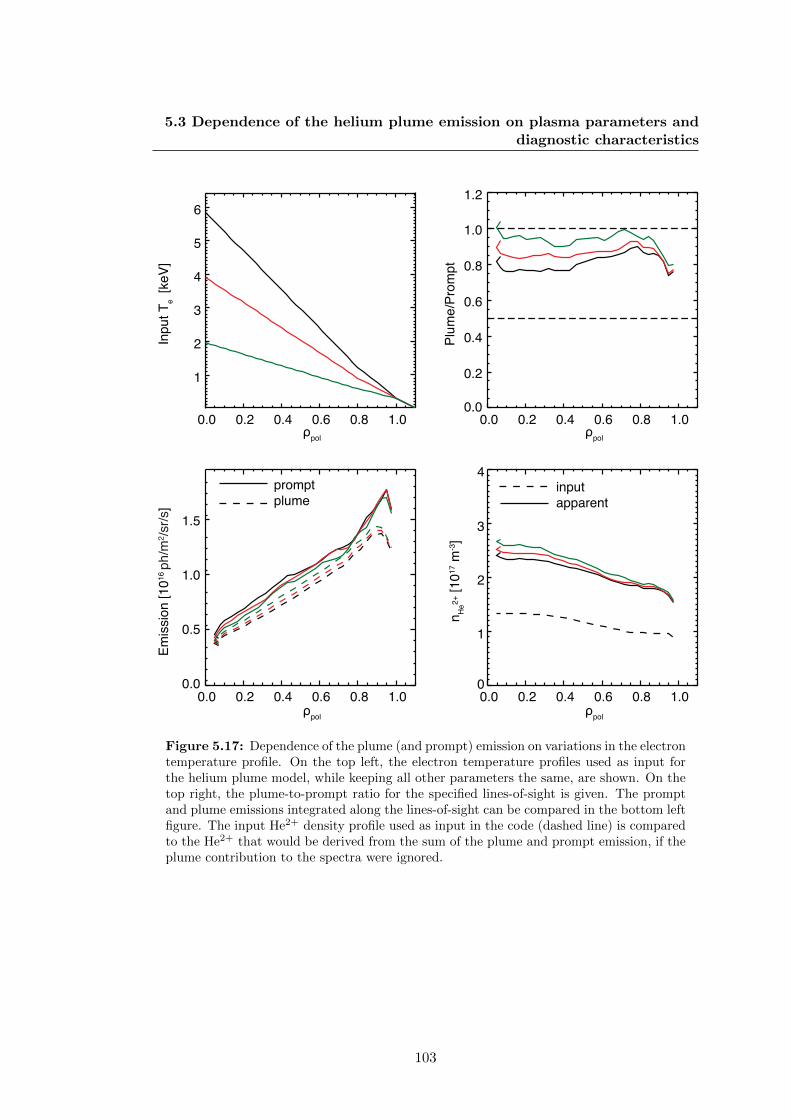
5.3 Dependence of the helium plume emission on plasma parameters anddiagnostic characteristics
Plu
me
/Pro
mp
t
0.0 0.2 0.4 0.6 0.8 1.0
1
2
3
4
5
6
0.0 0.2 0.4 0.6 0.8 1.00.0
0.2
0.4
0.6
0.8
1.0
1.2
0.0 0.2 0.4 0.6 0.8 1.00.0
0.5
1.0
1.5
0.0 0.2 0.4 0.6 0.8 1.00
1
2
3
4
ρpol
Input T
e
[ke
V]
ρpol
ρpol
ρpol
nH
e2
+ [10
17 m
-3]
prompt
plume
input
apparent
Em
issio
n [1
01
6 p
h/m
2/s
r/s]
Figure 5.17: Dependence of the plume (and prompt) emission on variations in the electrontemperature profile. On the top left, the electron temperature profiles used as input forthe helium plume model, while keeping all other parameters the same, are shown. On thetop right, the plume-to-prompt ratio for the specified lines-of-sight is given. The promptand plume emissions integrated along the lines-of-sight can be compared in the bottom leftfigure. The input He2+ density profile used as input in the code (dashed line) is comparedto the He2+ that would be derived from the sum of the plume and prompt emission, if theplume contribution to the spectra were ignored.
103

5. THE HELIUM PLUME EFFECT
5.4 Experimental investigation of the helium plume e↵ect
The existence of the helium plume emission in ASDEX Upgrade plasmas can be iden-
tified experimentally in two ways. First, via a comparison of the Ti and v� profiles
derived from the helium charge exchange measurements and those derived from mea-
surements on boron or carbon. Due to the plume emission, disagreement is expected,
since the helium plume emission originates from colder and slower plume ions belong-
ing to a di↵erent part of the velocity space (see Fig. 5.4). Second, by a comparison of
apparent helium density profiles from di↵erent geometries. The He2+ density profiles
derived from the charge exchange measurements without any treatment of the plume
e↵ect are expected to vary between di↵erent observation geometries, as the plume-to-
prompt intensity ratio depends on the diagnostic observation geometry (see Section
5.3.6). Both of these indications for the plume are observed at ASDEX Upgrade. For
example, in Fig. 5.18, the ion temperature and rotation profiles from helium and boron
are compared for ASDEX Upgrade discharge 29083 at 3.8s.
0.0 0.2 0.4 0.6 0.8 1.0ρ
pol
20
40
60
80
100
120
vφ [km
/s]
Helium
0.0 0.2 0.4 0.6 0.8 1.0
0.5
1.0
1.5
2.0
2.5
3.0
Ti [
ke
V]
ρpol
Boron Helium Boron
AUG 29083, t=3.8s
0 0
Figure 5.18: Comparison of rotation and ion temperature profiles obtained from mea-surements on helium and on boron. Strong discrepancies are observed, especially in theplasma core. The passive emission has been subtracted from the spectra.
The discrepancies in the ion temperature and rotation profiles are due to the non
Gaussian shape of the plume emission line that is part of the measured helium spectra.
The shape of this line depends strongly on the velocity, ion temperature and ionisation
time of the plume ion population that contributes emission to the measurement. The
plume emission line in the core will be wider, due to the higher temperature of the
plume ions, and shifted more to higher wavelengths than the plume emission line at
104

5.4 Experimental investigation of the helium plume e↵ect
0.0 0.5 1.0 1.5 2.0T
iB [keV]
0
20
40
60
(TiB-
TiH
e)/
TiB [%
]
0 20 40 60 80 100v
φB [km/s]
0
20
40
60
80
(vφ
B -
v φH
e)/
v φB [%
]
PECRH
> 0.8MWhelium gas puff
ρtor
=0.2ρ
tor=0.7
Figure 5.19: Comparison of toroidal rotation and ion temperatures at ⇢tor
= 0.2 and⇢tor
= 0.7 derived from helium and boron charge exchange measurements for all measure-ment time points in discharge 29083. Time points with additional ECRH power or closeto a helium pu↵ are indicated.
the edge. Due to the fact that an additional passive contribution from the plasma edge
complicates the analysis, all investigations have been performed with beam modulation
in order to unambiguously remove the passive emission line.
An overview of how strong this discrepancy due to the plume can be is obtained
by plotting the di↵erence of the Ti and v� values obtained from the percentage of the
Ti and v� values obtained from boron. In Fig. 5.19, all the time points from discharge
29083 are plotted. The time points during which additional ECRH power is applied and
the time points close to a helium pu↵ are identified. This discrepancy arises from the
plume emission line in the spectra which results from a complicated interplay of plasma
parameters. A larger discrepancy between the two ion temperature measurements is
observed in time points close to a helium pu↵, which can be attributed to the change in
the shape of the He2+ density profile. Smaller discrepancies in the ion temperature are
observed in the phases with additional ECRH, which shows that as plasma parameters
change, the spectral emission line changes as well by the interplay of lower ��, lower
Ti and higher Te. At outer regions of the plasma, the discrepancies are still significant,
especially for the rotation measurements.
105

5. THE HELIUM PLUME EFFECT
0.5 1.0 1.5 2.0 2.5 0
0.5
1.0
1.5
2.0
2.5
161
NBI #3
NBI #1
0.75 1.00 1.25 1.50 1.75 2.00 2.25 2.50
-1.0
-0.5
0.0
0.5
1.0
NBI #3
NBI #1NBI #1
toroidal LOS
poloidal LOS
poloidal LOS
toroidal LOS
Figure 5.20: Top down and poloidal view of ASDEX Upgrade, with the geometry of thetwo sets of LOS and the two beam sources used in the experiment.
Plasma discharge 29083 was specifically designed to benchmark the helium plume
model presented here. In this discharge, the helium spectra were measured using the
high etendue spectrometer described in Chapter 3 [79]. The spectrometer was connected
to two optical heads: one with predominantly toroidal LOS and one with more poloidal
LOS, all focussed on neutral beam source Q3 (see Fig. 5.20). The plume-to-prompt
intensity ratio is expected to be di↵erent for these two observation geometries, as the
path through the plume ion cloud is di↵erent.
The time traces of the most relevant plasma parameters during the discharge are
shown in Fig. 5.22. The experimental discharge was planned to have as stable plasma
conditions as possible. In addition, a specific scheme was implemented for the injection
of neutral beams. The neutral beam source (Q3) on which the helium and boron charge
exchange measurements were performed was modulated so that the passive emission
could be subtracted using the o↵-beam frames. The input power was kept constant by
supplementing Q3 with a source (Q5) on the other side of the torus. It should be noted
here that no plume ions originating at sources injected at the other side of the torus
(namely sources Q5-Q8) are expected to reach the spectrometer lines-of-sight.
106

5.4 Experimental investigation of the helium plume e↵ect
AUG 29083, t=2.555s
0 1 2 3 4distance along LOS [m]
0
2
4
6
8
Em
issi
on
[p
h/m
2/s
r/s]
Promptemission
Plume emission
Toroidal LOS
1016
0.0 0.5 1.0 1.5 2.0 2.5 3.0distance along LOS [m]
0
2
4
6
8
10
Em
issi
on
[p
h/m
2/s
r/s]
Prompt emission
Plume emission
Poloidal LOS
1016
Figure 5.21: Plume and prompt emission along a toroidal and a poloidal line-of-sight.
As an additional check, NBI source Q3 was replaced by NBI source Q1, for several
phases of the plasma discharge. NBI Q1 (also shown in Fig. 5.20) is more radial than
NBI Q3 and is situated below the toroidal lines-of-sight. Short helium gas pu↵s were
injected from a midplane valve, to increase the helium content and vary, albeit slightly,
the shape of the helium density profile.
In Fig. 5.23, the He2+ density profiles derived without taking into account the
plume e↵ect are shown on the left for both sets of lines-of-sight. It is observed that the
experimental density profiles measured by the poloidal and the toroidal lines-of-sight
do not agree. This is expected as the lines-of-sight have di↵erent geometries in relation
to the magnetic field lines and the neutral beam and are therefore a↵ected by the plume
di↵erently. The plume-to-prompt ratio for the toroidal lines-of-sight when NBIQ3 is
on is higher than the corresponding ratio for the poloidal lines-of-sight, as the path of
the poloidal lines-of-sight through the plume cloud is smaller than for the toroidal ones
(see also Fig. 5.24). In Fig. 5.21, the predicted prompt and plume emissions collected
along a line-of-sight are compared. The plume emission collected from a poloidal line-
of-sight is more localised and originates from the same volume as the prompt emission.
The toroidal line-of-sight, however, tranverses a longer path through the plume and,
therefore, plume emission is collected from an extended region.
Furthermore, the density profiles measured on NBI Q3 and NBI Q1 are also dif-
ferent, despite the fact that the plasma parameters are very similar. When NBI Q1
is on instead of NBI Q3, the situation changes. The toroidal lines-of-sight are above
107

5. THE HELIUM PLUME EFFECT
01
2
3
45
MW
PNBI
PECRH
Prad
0
1
2
3
MW
Q1
Q3
Q5
02
4
6
8
10
19 m
-2
H1
H5 H2
0.0
1.0
2.0
3.0
ke
V
Ti @2.0m
Ti @1.73m
Te(0)
0
50
100
150200
km
/s
vrot
@2.0m
vrot
@1.73m
AUG 29083
0
0 2 4 6 8Time (s)
01
2
3
45
10
21 /
s
He
Dtot
(a)
(b)
(c)
(d)
(e)
(f )
Figure 5.22: Time traces of the relevant parameters for discharge 29083: a) injectedand radiated power, b) details of the NBI replacement scheme, c) line integrated electrondensity, d) electron and ion temperatures, e) plasma rotation, f) total deuterium and heliumgas pu↵s.
the center of NBI Q1 and only view the edge of this source. As such, the prompt
CX signal is lower for the toroidal lines-of-sight (by approximately a factor of 3 in
the core). However, the toroidal lines-of-sight still measure plume ions produced by
NBI Q1 which have followed the magnetic field lines into the lines-of-sight. In this
case, the plume-to-prompt ratio in the core is almost a factor of 2 higher than for NBI
Q3. The poloidal lines-of-sight barely intersect NBI Q1 and measure almost exclusively
the plume originating from NBI Q1. The calculated plume-to-prompt ratio is indeed
approximately 10 times higher in comparison to the ratio for the NBI Q3 time point
(shown divided by 10 in Fig. 5.24).
In the right plot of Fig. 5.23, however, the He2+ density profiles corrected with the
plume emission model presented here are shown. The corrected densities are obtained
by multiplying the densities in the left plot with a factor of 1/(1 + R), where R is the
108

5.5 Reconstruction of the helium spectrum
0.0 0.2 0.4 0.6 0.8 1.0ρ
pol
0
2
4
6
8
10
12
nH
e2
+ [
10
17
m-3
]
0.0 0.2 0.4 0.6 0.8 1.0ρ
pol
0
2
4
6
8
10
12
nH
e2
+ [
10
17
m-3
]
He2+ density He2+ densityplume corrected
29083, t=2.565s, 2.965s 29083, t=2.565s, 2.965s
poloidal LOS NBI #3
toroidal LOS NBI #1
poloidal LOS NBI #1
toroidal LOS NBI #3
Figure 5.23: He2+ density profiles obtained from CX measurements for the ASDEXUpgrade discharge 29083 at 2.565s (NBI Q3 on) and at 2.975s (NBI Q1 on) without theplume e↵ect taken into account and the corrected profiles after the plume e↵ect has beenmodelled, for the toroidal and poloidal viewing geometry.
ratio of plume emission signal integrated along each line-of-sight to the active CX signal,
shown in Fig. 5.24. The corrected density profiles from the toroidal and the poloidal
lines-of-sight are now in much better agreement. In addition, as the plasma parameters
are similar between the NBI Q1 and NBI Q3 phases, the He2+ density profile from the
NBI Q1 phase can be compared to the profile measured on NBI Q3. Good agreement
is found in this case as well. Part of the remaining discrepancies can be attributed to
intensity calibration uncertainties between the two optical heads. As the uncertainties
(see error bars in the right plot in Fig. 5.23) may play an important role, the ultimate
test of the plume model is whether the line shape of the spectral plume emission can
be predicted.
5.5 Reconstruction of the helium spectrum
The model for the helium plume emission provides not only a spatial distribution of
the plume ions, but also information on their velocity. It is, therefore, possible to
reconstruct the plume emission spectral line. In this section, the reconstruction of
the plume emission line is described which, together with the modelled active emission
109

5. THE HELIUM PLUME EFFECT
0.0 0.2 0.4 0.6 0.8 1.00.0
0.5
1.0
1.5
2.0
Plu
me
/Pro
mp
t
ρpol
poloidal LOS NBI #3
toroidal LOS NBI #1
poloidal LOS NBI #1 [/10]
toroidal LOS NBI #3
Figure 5.24: The plume-to-prompt intensity ratios calculated for the helium densitymeasurements shown in Fig. 5.23.
line, can be compared to the experimental measurements. Apart from o↵ering a further
benchmarking of the helium plume model, modelling the helium plume emission line
itself can ultimately allow for the derivation of accurate ion temperature and rotation
profiles from the helium charge exchange spectra.
As already discussed in the previous section, it has been observed at ASDEX Up-
grade, where charge exchange measurements on more than one impurity are routinely
performed, that the ion temperature and rotation profiles derived from the HeII line
di↵er from those measured on the BV or CVI lines if the plume emission line is not
corrected for. Assuming that both the passive emission line and the plume emission
line are correctly subtracted from the measured spectra, the remaining spectral shape,
which is the isolated active charge exchange emission line, should yield ion temperature
and rotation profiles that compare well with the boron or carbon measurements. The
passive emission line is removed by means of subtracting passive frames during which
the neutral beam is switched o↵, while the plume emission line shape is modelled.
The helium plume model provides the modelled active (prompt) line and the mod-
elled plume emission lines, the sum of which can be compared with the measurements.
The prompt emission line for each measurement location is represented by a single
110

5.5 Reconstruction of the helium spectrum
Gaussian shape, with a line shift �� and a line width �:
�� =vBrot�0
cos(�)
c
� =
sTBi k
mc2�0
,
(5.18)
where �0
is the natural wavelength (468.571nm) and � is the angle between the line-of-
sight and the toroidal direction. The superscript B denotes that boron measurements
are used for the Ti and v� values at this location.
The plume emission line, on the other hand, can not be described by a single
Gaussian, due to the non-Maxwellian e↵ects described in Section 5.2. Additionally, the
emission comes from many locations along the line-of-sight, which are characterised by
di↵erent Ti and v� values. Similar to the description of the active charge exchange
emission line given in Chapter 3, the observed spectral plume intensity in terms of
velocities along the line-of-sight and for each location along the line-of-sight (l) is given
by an equation of the following form:
Iplume(��, l) =1
4⇡ne(l)Q
eexc(l)dl
Z
�x
Z
�y
Z
�z
fHe+(l, �x, �y, �z)�(����!� ·cos ✓)d�xd�yd�z,
(5.19)
where �!� is the ion velocity, ✓ the angle between the ion velocity and the line-of-sight
(z-axis) and l gives the coordinate along the line-of-sight. The helium plume ions are
described by the velocity distribution fHe+(l, �x, �y, �z) obtained by the Monte Carlo
simulation.
The Monte Carlo modelling provides directly the distribution of the helium plume
ions also in velocity space. The plume ion density is given in terms of velocities along
each magnetic field line. Assuming that � is the angle between line-of-sight and the
magnetic field line, the velocity is projected along and perpendicular to the line-of-
sight as �k,los = �k,�!B cos(�) and �?,los = �k,�!B sin(�), respectively. The plume spectrum
is then reconstructed using Eq. (5.19), with fHe+(l, �k,los, �?,los), obtained from the
Monte Carlo simulation.
To extract accurate He2+ density profiles, the modelling of the helium plume line
and the comparison of the modelled emission lines with the spectra has to be iterated.
As already described in Section 5.3, the plume emission depends on the shape of the
111

5. THE HELIUM PLUME EFFECT
AUG 29083, t=2.575s
467 468 469 470 471wavelength [nm]
0
1
2
3
4
5
6
IC
X [10
16
ph
/m2/s
r/s]
Total modelledspectrum
Plume emissionmodelled
Active CX modelled
Measured spectrum
(passive CX subtracted)
ρpol
=0.27
467 468 469 470 471wavelength [nm]
0
1
2
3
I CX [10
17
ph
/m2/s
r/s]
Total modelledspectrum
Plume emissionmodelled
Active CX modelled
Measured spectrum
(passive CX subtracted)
ρpol
=0.93
AUG 29083, t=2.575s
Figure 5.25: Reconstruction of helium charge exchange spectra for the toroidal viewinggeometry, for discharge 29083, t=2.575s using the Monte Carlo method, for a core (left)and an edge line-of-sight (right). Very good agreement is found between the sum of thereconstructed prompt and plume emission lines and the measured spectra, from which thepassive emission has been subtracted.
He2+ density profile. Since this is an input to the modelling, comparison of the out-
put modelled emission lines with the spectra is required and more iterations might be
necessary. In simple words, an assumed He2+ density profile is used as input to the
model: either the He2+ densities calculated ignoring the contribution of the plume or
He2+ density profiles that follow the shape of the electron density profile can be used.
The plume and prompt emission lines are reconstructed and compared to the mea-
sured spectra. A scaling factor is applied to the modelled emission lines to match the
measurement, same for both emission lines, but possibly di↵erent between the di↵er-
ent lines-of-sight. If the normalised residuals between the modelled and the measured
spectrum are not satisfactory, the model is iterated once more, taking into account the
scaling factors. The process can be repeated as many times as required to minimise
the di↵erence between the modelled and the measured spectrum, but good agreement
is typically found within 2-3 iterations, within the error bars of the measured spectrum
and the He2+ density profiles.
In Fig. 5.26, measured ion temperature and rotation profiles of boron and helium
are shown. The helium spectra fitted with a single Gaussian (passive subtracted using
beam modulation) are shown in red. In addition, the modelled profile of the plume
component is plotted in green, also fitted with one Gaussian. In blue, the profiles
obtained from boron measurements and used as input to the modelling, are plotted.
112

5.6 Considerations on the plume e↵ect
0.0 0.2 0.4 0.6 0.8 1.0ρ
pol
0
1
2
3
4
Ti [k
eV
]
Helium Plume
0.0 0.2 0.4 0.6 0.8 1.00
50
100
150
vφ [km
/s]
Boron
Helium (apparent)
Helium - Plume subtracted
ρ pol
Figure 5.26: Reconstructed ion temperature and rotation profiles for the toroidal viewinggeometry, for discharge 29083, t=2.565s. The profiles derived from boron measurementsare shown in blue and the ones derived from helium measurements, without correctingfor the plume are shown in red. The plume profiles derived from fitting the plume withone Gaussian are shown in green. The profiles derived from helium measurements aftercorrecting for the plume are shown in magenta.
The modelled plume emission line is subtracted from the helium spectra, which are
subsequently fitted with a Gaussian, resulting in the profiles shown in magenta. Very
good agreement is found with the boron measurements. Ultimately this means that the
plume model describes the involved physics to a high degree of accuracy, because not
only the relative size of plume to prompt emission is described, but also the distribution
of the plume in velocity space is matched. Thus, the observed di↵erences in the He2+
density encountered in Fig. 5.23 are probably given by instrumental uncertainties rather
than by the plume model.
5.6 Considerations on the plume e↵ect
In the past, a number of studies have been conducted in order to understand the
helium plume e↵ect and to model the helium plume emission. The helium plume e↵ect
was first described and named by Fonck et al in [9]. In this paper the helium plume
e↵ect is identified as a significant disturbance to the helium charge exchange spectra.
A simplified model for the evaluation of the plume emission is proposed assuming
113

5. THE HELIUM PLUME EFFECT
one dimensional transport along a magnetic field line. The dependence of the plume
emission on parameters such as the diagnostic observation geometry and the beam
energy is described. It is also noted that no accurate toroidal rotation profiles can
be obtained from the helium charge exchange spectra, if the plume e↵ect is not taken
into account. Gerstel et al attempted in [121], to calculate both the plume from the
thermal helium content in the plasma, but also the helium beam “plume”, as part
of the analysis of helium beams. Here a Monte Carlo approach was employed for
solving the transport equation of the hydrogenic plume ions. Nevertheless, the helium
plume emission is not shown to be taken into account in the fitted helium spectra.
In [56], it is mentioned that the plume emission calculated from the model in [121]
is overestimated by a factor of 3 in intensity. The helium plume emission was also
studied at DIII-D [122], following a method similar to the one described in [9] as well
as considering a Maxwellian distribution to describe the plume ions. Here, the plume
emission corrections are found to be important only in terms of magnitude, but not
significant in terms of profile shapes. A further e↵ort to model the helium plume can
be found in [105], where the method found in [9] is also followed.
In this work, the plume e↵ect has been confirmed to be a significant contribution in
the helium charge exchange spectra. The plume emission contribution in the spectrum
is complicated and depends on a number of plasma parameters, as well as on the
diagnostic geometry, and needs to be treated appropriately. Accurate He2+ density
profiles can be derived only if the plume emission is modelled and subtracted from the
measured spectra.
Furthermore, it should be noted that the helium plume e↵ect is important across
the whole plasma radius, including the plasma edge. However, as the plume emission
line has an apparent lower temperature and velocity than the active charge exchange
line, it can easily be mixed with the passive emission line depending, of course, on the
viewing geometry and edge plasma parameters. Furthermore, the helium plume e↵ect
can be minimised with the use of poloidal views, but still not avoided completely.
For the first time the non-Maxwellian features of the plume emissions from the
same plasma radius have been implemented, which resulted in the breakthrough for
the modelling not only the helium plume-to-prompt ratio but also for the modelling of
the detailed charge exchange including plume and prompt components.
114

5.6 Considerations on the plume e↵ect
Pushing the helium plume model further and starting from the measured helium
charge exchange spectra and the derived Ti and v� values, which as described are
a↵ected by the helium plume emission, an iterative modelling process could be imple-
mented so as to converge to accurate Ti and v� profiles. This would allow for standalone
charge exchange measurements based on the HeII line, without the need for input from
other impurity measurements for the modelling of the plume emission.
Looking ahead at future fusion machines, for example ITER, the helium plume ef-
fect must be taken into account as charge exchange spectroscopy is expected to provide
measurements of the helium “ash”. Both the electron impact excitation rates and the
electron impact ionisation rates will be lower at the higher electron temperatures of
ITER, meaning in general lower plume emission intensities with the increasing elec-
tron temperature. The higher electron densities mean shorter ionisation lengths for
the He+ ions, while the electron impact excitation rates drop with increasing density,
resulting again into smaller contributions from the plume. In ITER conditions how-
ever, ion impact ionisation will also become important. The lines-of-sight of the charge
exchange diagnostic on ITER are designed to view the neutral beam with angles almost
perpendicular to the magnetic field lines, in order to minimise the helium plume con-
tribution [82]. Nevertheless, it is certain that the helium plume e↵ect will be important
for the thermal helium charge exchange measurements on ITER, but the magnitude of
this e↵ect has yet to be estimated.
115

5. THE HELIUM PLUME EFFECT
116

6
Investigation of the thermal
helium transport in ASDEX
Upgrade plasmas
3.1 Components of a charge exchange spectrum
3.1.1 Active charge exchange emission
3.1.2 Passive charge exchange and edge emissions
3.1.3 Bremsstrahlung background
3.1.4 Contribution from the beam halo
3.1.5 Plume emission
3.1.6 Contributions from other impurities
3.1.7 Fast ion tail
3.2 Charge exchange recombination spectroscopy as a
plasma diagnostic
3.2.1 Physical quantities from CX spectra
3.2.2 Derivation of impurity density profiles
3.2.3 Charge exchange cross sections and cross section e↵ects
3.2.4 Charge exchange spectroscopy for fast ions
3.3 CXRS diagnostic instrumentation at ASDEX Upgrade
3.3.1 Calibration of CXRS measurements
The shape of the helium density profile in future fusion reactors will have a serious
e↵ect on their performance, due to helium “ash” accumulation issues. To predict how
117

6. INVESTIGATION OF THE THERMAL HELIUM TRANSPORT INASDEX UPGRADE PLASMAS
the helium density profile will behave, understanding of the helium transport in fu-
sion plasmas and experimental validation of the current theoretical understanding are
required. This is the objective of this chapter. Here, the helium density profiles mea-
sured in ASDEX Upgrade will be systematically compared to the available theoretical
predictions to validate the theory and shed light on the behaviour of helium in future
devices.
Previous investigations of helium transport at DIII-D have shown that the helium
density profile has a similar shape to the electron density [122]. At ASDEX Upgrade
helium transport studies have not previously been done, but boron studies showed that
the normalised logarithmic boron density gradients can be qualitatively reproduced by
gyrokinetic modelling if the “roto-di↵usive” term, proportional to the normalized gra-
dient of the toroidal rotation, is included [11, 27] as discussed in Section 4.3. Moreover,
previous gyrokinetic simulations of helium indicate that the thermodi↵usive contri-
bution to the particle flux should be more important for helium than for higher-Z
impurities such as boron, leading to di↵erent peaking of the two profiles [114].
Taking these works into account, dedicated experiments optimised for both helium
and boron charge exchange measurements were performed at ASDEX Upgrade to deter-
mine the experimental correlation of these impurity density gradients with theoretically
relevant plasma parameters, namely: the normalized gradients of the electron density,
the ion temperature and the toroidal rotation. Systematic studies dedicated to multi-
ple impurities simultaneously, such as the one presented here, are necessary in order to
have a deeper investigation of the transport physics of these species. Assessing the ap-
plicability of the present theoretical models for impurity transport to the experimental
observations is very important as such studies allow a more stringent validation of the
theoretical predictions.
This study focusses on the confinement region (mid-radius), where neoclassical
transport is expected to be negligible and turbulent transport is expected dominate.
The database collected for this study and the experimental observations are described
in Sections 6.1 and 6.2. Then the experimental data are compared to the theoreti-
cal predictions in Section 6.3. The neoclassical contributions to the helium and boron
transport are discussed and compared with the transport due to the electrostatic plasma
turbulence. Detailed comparisons of the measured impurity density gradients with gy-
118

6.1 Database for the investigation of helium transport
rokinetic simulations of the turbulent transport are presented. Conclusions are drawn
in Section 6.4.
6.1 Database for the investigation of helium transport
A database of helium and boron density profiles was assembled from a set of exper-
iments performed at ASDEX Upgrade designed specifically for the investigation of
helium transport. The plasma discharges were optimised for helium and boron charge
exchange measurements. The experiments were performed soon after a boronisation
(coating of wall components produced by a glow discharge with 10% B2
D6
and 90%
He [123]), to ensure very good charge exchange signal from both impurities. Fresh
boronisation also enables the performance of low density, low collisionality plasmas.
The charge exchange measurements are performed on NBI Q3 of ASDEX Upgrade,
with two di↵erent spectroscopic instruments, boron measurements performed with the
spectrometer described in [63] and helium measurements performed with the system
described in Section 3.3. Both measurements extend from the plasma center to approx-
imately ⇢tor = 0.85. The NBI source was modulated and replaced by another injection
source at the other side of the torus, so as to enable the subtraction of the passive emis-
sions and reduce the uncertainties in the interpretation of the helium charge exchange
spectra while keeping the total injected power constant.
All six discharges included in this database were performed at a plasma current
of 600kA and a magnetic field of 2.5T. The goal of these discharges was to provide
optimised boron and helium density profiles together with scans of the experimental
parameters expected to be relevant to the impurity transport in di↵erent turbulence
regimes, namely the collisionality and the normalised gradients of the electron density,
the ion temperature and the toroidal rotation. Di↵erent levels of electron cyclotron
and neutral beam heating were applied in order to perform a scan of R/Lne , R/LTi ,
the radial gradient of the toroidal plasma velocity u0 and ⌫e↵
, where ⌫e↵
is the e↵ective
collisionality, defined as the ratio of the electron-ion collision frequency to the curvature
drift frequency.
The application of central electron cyclotron heating has clear e↵ects on the electron
density profile, causing strong peaking as the plasma turbulence regime transitions from
ITG to TEM [27]. Furthermore, central deposition of ECRH leads to flat and even
119

6. INVESTIGATION OF THE THERMAL HELIUM TRANSPORT INASDEX UPGRADE PLASMAS
Table 6.1: Parameter space covered in the helium transport database presented in thiswork at ⇢
tor
= 0.5.
Parameter Value range Parameter Value rangeR/Lne 0.03-3.6 ne(⇢tor = 0) 5� 8 · 1019m�3
R/LTe 3.5-7 Te(⇢tor = 0) 2� 6keVR/LTi 3.0-7 Ti(⇢tor = 0) 0.8� 2.3keVu0 -0.15-1.1 v�(⇢tor = 0) 20� 140km/s⌫e↵
0.3-1.9 q95
6.9-7.4
hollow rotation profiles, an e↵ect connected again to the plasma turbulence [124, 125].
A scan in NBI power was also performed to vary the Mach number, also using a
combination of on- and o↵-axis beams in an attempt to vary the admittedly very sti↵
ion temperature profile. Di↵erent levels of deuterium fuelling were also used during
one discharge to change the collisionality. The heating schemes of discharges 30367
and 30379 are shown in Fig. 6.1 as examples. They feature a scan of ECRH power in
the first case and a scan of NBI power in the second discharge. Averaged profiles are
shown for four example phases.
A total of 131 steady state phases 55-110ms long were selected out of these dis-
charges to form the database analysed here. The data points selected have been ELM-
synchronised when ELMs were present, to avoid the strong e↵ect of ELMs on the
profiles. With the exception of discharge 29083, no strong sawteeth were documented
in this database. When present, the sawteeth existed in the core, with an inversion
radius ⇢tor < 0.2. Furthermore, no modes were present.
An overview of the parameter space explored is shown in Fig. 6.2, with further
details given in Table 6.1 for ⇢tor = 0.5. We succeeded in varying the collisionality
⌫e↵
at ⇢tor = 0.5 by a factor of 6, with a variation of the core electron density from
5 to 8 · 1019m�3 and core electron temperature from 2 � 6keV . A factor of 3 in the
variation of deuterium Mach number at ⇢tor = 0.5 was achieved (0.08 � 0.26). The
applied electron heating power ranges from 0 to 4MW and the NBI power 0�7.5MW .
In comparison to previous work investigating light impurity transport (boron) [11],
similar ranges in R/Lne and R/LTi were achieved, but narrower ranges of R/LTe and
u0 (approximately 4 � 10 and �0.5 to 3, respectively, in [11]). The q95
values are on
the higher end of the q95
values in [11] (q95
= 4� 7).
The impurity density profiles were evaluated from the measured charge exchange
120

6.1 Database for the investigation of helium transport
0.0
1.0
2.0
3.0
Q3
Q5
0.0
1.5
PECRH
30367
0.0
1.0
2.0
3.0
Q3
Q5
PECRH
0 2 4 6 8Time (s)
30379
Q6Q7
Q3+Q5+Q7Q3+Q7
02468
Q3
PNBI
0 2 4 6 8Time (s)
0.51.0
PN
BI [
MW
]P
EC
RH [
MW
]P
NB
I [M
W]
Ph
eat
ing [
MW
]
0
1
2
3
4
0
2
4
6
ne [1019 m-3]
0.0 0.2 0.4 0.6 0.8 1.00
20
40
60
80
100v
φ [km/s]
ρtor
Te [keV]
Ti [keV]
Q3+Q5
(b)
(a)
Figure 6.1: Heating schemes of two discharges from the helium transport database. a)In discharge 30367, a scan of ECRH power at constant NBI power was performed, in orderto vary the peaking of the electron density profile. b) In discharge 30379, a scan of NBIpower at constant ECRH power was performed, in order to see the e↵ect of on- and o↵-axisbeams and NBI power levels on the impurity density profiles.
intensities, using the charge exchange impurity concentration analysis code CHICA,
which uses the Monte Carlo neutral beam simulation code FIDASIM [69, 74] for the
neutral beam attenuation calculations, including the beam halo. The evaluation of
the helium density profiles takes into account the plume emission, using the plume
emission forward model described in Chapter 5. Electron density and temperature
profiles derived from IDA (see Section 2.3.5) and ion temperature and rotation profiles
measured on boron have been used as input to the impurity concentration analysis code
and to the plume modelling code.
121

6. INVESTIGATION OF THE THERMAL HELIUM TRANSPORT INASDEX UPGRADE PLASMAS
0.0 0.5 1.0 1.5 2.0νeff
0
1
2
3
4
R/Lne
3036730368303743037930380
29083
0.0 0.5 1.0 1.5 2.02
3
4
5
6
7
8
R/LTi
0.0 0.5 1.0 1.5 2.0-0.2
0.0
0.2
0.4
0.6
0.8
1.0
1.2
u'
ρtor
=0.5
νeff
νeff
(a) (b) (c)
Figure 6.2: Overview of the parameter space in the helium transport database analysedin this work, namely the normalised logarithmic gradients of a) electron density and b) iontemperature and c) the radial gradient of the toroidal plasma velocity as a function of thee↵ective collisionality.
6.2 Experimental observations
In the investigated discharges we obtained a wide variety of experimental helium and
boron density profiles. Examples of the profiles are shown in Fig. 6.3. These time points
are also indicated in the database in Fig. 6.2. In the database, the helium profiles are
observed to vary from extremely flat to very peaked profiles, but it does not become
hollow. The boron profiles on the other hand are observed to vary from slightly hollow
to very peaked.
The normalised gradients of the impurity and electron density profiles at two plasma
locations, namely at ⇢tor = 0.3 and ⇢tor = 0.5 are shown in Fig. 6.4. At ⇢tor = 0.5, the
helium and boron impurity gradients are comparable to the electron density gradient,
similar to what was observed at DIII-D [122]. At ⇢tor = 0.3, the impurity profiles
are generally less peaked than the electron density, with the exception of helium at
high R/Lne values. While one might naively assume that the helium profiles should
lie between the electron density and boron profiles, it is observed that this is not the
case, indicating complex mechanisms at play. The error bars plotted in Fig. 6.4 take
into account the density profile measurement uncertainty, but not the error from the
fitting procedure.
Previous work [11] illustrated the importance of u0 on the boron profile. In Fig. 6.5,
R/LnZ is plotted versus u0, showing that it decreases with increasing u0. However,
the interpretation is not so simple as other plasma parameters are changing at the
122

6.3 Comparison to impurity transport theory
0.0 0.2 0.4 0.6 0.8 1.00
1
2
3
4
5
nH
e2
+ [10
17m
-3]
0.0 0.2 0.4 0.6 0.8 1.0ρ
tor
0
2
4
6
8
10
R/L
nH
e2
+
0.0 0.2 0.4 0.6 0.8 1.00
1
2
3
4
5
nB
5+ [10
17m
-3]
0.0 0.2 0.4 0.6 0.8 1.0-1
0
1
2
3
R/L
nB
5+
ρtor
ρtor
ρtor
30368, t=6.7675s30368, t=7.8275s
30368, t=6.7675s30379, t=5.8675s
Figure 6.3: Example profiles of helium (left) and boron (right) shown together with thenormalised logarithmic impurity density gradients (bottom plots).
same time. As the impurity density profiles at a certain location in the plasma are
determined by the interplay of many parameters, it is not straightforward to disentangle
the dependencies.
To try and better identify the underlying physics mechanisms at work, theoretical
simulations of the neoclassical and turbulent transport expected in these plasmas have
been performed and compared to the experiment. This is presented in the next section.
6.3 Comparison to impurity transport theory
6.3.1 Neoclassical transport contributions
All of the points in the database have been modelled with the neoclassical transport
code NEOART [89, 90]. Neoclassical transport is expected to be negligible around
123

6. INVESTIGATION OF THE THERMAL HELIUM TRANSPORT INASDEX UPGRADE PLASMAS
1.0 1.5 2.0 2.5 3.0 3.5 4.0 4.5
R/Lne
-1
0
1
2
3
4
R/L
nZ
He
B
0 1 2 3 4
-1
0
1
2
3
4
R/Lne
ρtor
=0.3 ρtor
=0.5R
/Ln
Z
Figure 6.4: Experimentally deduced R/LnB
and R/LnHe
at ⇢tor
= 0.3 and ⇢tor
= 0.5.
u’
R/L
nZ
He
B ρtor
=0.3 ρtor
=0.5
-0.5 0.0 0.5 1.0 1.5 2.0
-1
0
1
2
3
-0.2 0.0 0.2 0.4 0.6 0.8 1.0 1.2-1
0
1
2
3
4
R/L
nZ
u’
Figure 6.5: Experimentally deduced R/LnB
and R/LnHe
as a function of u0 at ⇢tor
= 0.3and ⇢
tor
= 0.5.
mid-radius [25, 27] in comparison to the turbulent contributions, nevertheless, this has
to be confirmed also for the current database.
The di↵usion coe�cients and drift velocities for helium and boron at ⇢tor = 0.3 and
⇢tor = 0.5 derived from NEOART are shown for all time points as a function of the ratio
of electron to ion temperature Te/Ti in Fig. 6.6. The neoclassical drift velocities, shown
on the right of Fig. 6.6, are generally directed inward at both locations and for both
124

6.3 Comparison to impurity transport theory
impurities, providing a balance against the di↵usion. The only exception is for boron
at low Te/Ti. Here, the drift is also outward at mid-radius, meaning that if neoclassical
transport is important then these points (highlighted in green) should feature hollow
profiles. The actual R/LnB profiles corresponding to these points however, have values
of 0.4-2.4, indicating that neoclassical transport is not the only mechanism here.
1.0 1.1 1.2 1.3 1.4 1.5 1.6 1.70.00
0.05
0.10
0.15
0.20
0.25
-0.7
-0.6
-0.5
-0.4
-0.3
-0.2
-0.1
ne
ocl
ass
ica
l d
iffu
sio
n [m
2/s
]
HeB
1.0 1.1 1.2 1.3 1.4 1.5 1.6 1.7T
e/T
i
ne
ocl
ass
ica
l d
rift [m
/s] He
B
Te/T
i
ρtor
=0.3 ρtor
=0.3
1.0 1.1 1.2 1.3 1.4 1.5 1.6 1.70.00
0.05
0.10
0.15
ne
ocl
ass
ica
l d
iffu
sio
n [m
2/s
]
HeB
1.0 1.1 1.2 1.3 1.4 1.5 1.6 1.7T
e/T
i
-0.4
-0.3
-0.2
-0.1
0.0
0.1
0.2
ne
ocla
ssic
al d
rift [m
/s]
Te/T
i
HeB
ρtor
=0.5 ρtor
=0.5
outwardinward
Figure 6.6: Neoclassical di↵usion and convection for boron (blue) and helium (red) in thetransport database for ⇢
tor
= 0.3 (top) and ⇢tor
= 0.5 (bottom). For ⇢tor
= 0.5, the caseswhere the Pfirsch-Schluter contribution to the boron di↵usion is larger than the banana-plateau contributions are identified with green (DPS > 1.3DBP ). The arrows indicate thecases of interest that are examined in Fig. 6.7.
Generally we see that di↵usion of helium and boron in the plasma core is dominated
by the banana-plateau contribution, while the edge by the Pfirsch-Schluter contribution,
as can be seen in Fig. 6.6, where the radial profiles of the neoclassical coe�cients are
125

6. INVESTIGATION OF THE THERMAL HELIUM TRANSPORT INASDEX UPGRADE PLASMAS
0.2 0.4 0.6 0.8ρ
tor
0.00
0.05
0.10
0.15
0.20
0.25
ne
ocla
ssic
al d
iffu
sio
n [m
2/s
]
Total
BP
PS
CL
-0.4
-0.2
0.0
0.2
0.4
0.0
0.1
0.2
0.3
0.4
-0.5
-0.4
-0.3
-0.2
-0.1
0.0
ne
ocla
ssic
al d
rift [m
/s]
ne
ocla
ssic
al d
iffu
sio
n [m
2/s
]
ne
ocla
ssic
al d
rift [m
/s]
0.2 0.4 0.6 0.8ρ
tor
0.2 0.4 0.6 0.8ρ
tor
0.2 0.4 0.6 0.8ρ
tor
30379, 2.75s
30368, 2.81s
He He
B B
Figure 6.7: Neoclassical di↵usion and convection coe�cients for boron (top row) andhelium (bottom row) in 30368 at 2.81s (solid lines) and 30379 at 2.75s (dashed lines). BP,PS and CL correspond to the banana-plateau, Pfirsch-Schluter and classical contributions,respectively.
shown. The cases with outward boron drift correspond to cases where the Pfirsch-
Schluter contribution is larger than the banana-plateau one (dashed lines). The outward
drift velocities of boron at ⇢tor = 0.5 can be explained by considering the temperature
screening e↵ect. Not only is the temperature screening e↵ect weaker for helium [93],
but the temperature screening is also stronger in the Pfirsch-Schluter regime that is
more relevant for boron. To test this explanation, a temperature screening factor fTS
can be derived from Eq. (4.9), defined as the multiplication factor of the temperature
126

6.3 Comparison to impurity transport theory
1.0 1.1 1.2 1.3 1.4 1.5 1.6 1.7T
e/T
i
0
1
2
3
4
NC
diff
usi
on
ra
tio B
P/P
S
HeB
ρtor
=0.5
Figure 6.8: Ratio of the banana-plateau to Pfirsch-Schluter di↵usion coe�cients for boronand helium at ⇢
tor
= 0.5. The cases where the boron drift velocity is directed outwardsare indicated with green.
gradient:
� = �CL + �PS + �BP =
= Z⇥DCL(n0 + fCLT 0) +DPS(n0 + fPST 0) +DBP (n0 + fBPT 0)
⇤
= Z⇥(DCL +DPS +DBP )n0 + (DCLfCL +DPSfPS +DBP fPS)T 0⇤ ,
(6.1)
where n0 and T 0 stand for the gradients of the density and temperature, respectively.
The temperature screening factors fCL,fPS ,fBP , defined for each neoclassical contribu-
tion, give the total temperature screening factor fTS = DCLfCL+DPSfPS+DBP fPS .
To illustrate the di↵erent e↵ect of the temperature screening on helium and boron,
the �/D ratios, normalised with Z, are plotted in Fig. 6.9, for a small subset of the
database. The contribution of the density gradient (triangles) and the contribution of
the temperature gradient (diamonds) are shown. The density contribution is the same
for both impurities. As expected, the temperature gradient contribution in the case of
helium is smaller than that of boron but not by much. The total drift parameter �/D,
normalised over Z, does become positive for boron (for Te/Ti ⇠ 1.1), which would mean
hollow boron profiles, if neoclassical transport was the only contribution.
127

6. INVESTIGATION OF THE THERMAL HELIUM TRANSPORT INASDEX UPGRADE PLASMAS
1.0 1.1 1.2 1.3 1.4 1.5 1.6 1.7-2.5
-2.0
-1.5
-1.0
-0.5
0.0
0.5
1.0
(υ/D
)NC/Z
[m
-1]
Te/T
i
n‘ term
T‘ term
total
HeB ρ
tor=0.5
Figure 6.9: Drift parameters �/D for helium and boron for a subset of the database,normalised over Z. The contributions of the density gradient (4) and temperature gradient(⌃) are indicated separately (see Eq. (6.1)).
Impurity density profile gradients calculated taking only the neoclassical transport
into account are compared with those obtained from the experiment at ⇢tor = 0.5 in
Fig. 6.10. As expected for this location, neoclassical transport does not seem able
to explain the measurement. It predicts R/LnB in the range of �5 to 10, which are
not observed in the experiment. The neoclassical prediction for helium seems better
in comparison to the boron, as the boron drift velocities cover a much wider range.
However, even if the neoclassical prediction for �/D appears good, the absolute values
of � and D are also important as they include also a turbulent part.
In the next section, the neoclassical coe�cients calculated here are compared with
the contribution of turbulent di↵usion and convection, which are expected to be the
dominant terms defining the transport of helium and boron at mid-radius, to assure
that the neoclassical contribution is negligible and can be ignored in the analysis.
6.3.2 Turbulent contributions
Turbulent transport modelling
The modelling of the turbulent transport in the database has been performed with
the gyrokinetic simulation code GKW [126, 127]. GKW is a nonlinear gyrokinetic flux
128

6.3 Comparison to impurity transport theory
R/L
nZ
(exp
erim
en
t)
ρtor
=0.5
R/LnZ (Neoclassical)
-5 0 5 10-1
0
1
2
3
HeB
Figure 6.10: R/LnB
and R/LnHe
from the experiment are compared with the predictionbased on neoclassical transport alone, at ⇢
tor
= 0.5.
tube code and simulates the tokamak plasma microinstabilities and turbulence. The
gyrokinetic equation [114] is solved and the normalised logarithmic impurity density
gradients are derived by setting the impurity particle flux to zero. The rotodi↵usive
contribution to the turbulent transport, as well as the coriolis force are included [115,
127–129]. Centrifugal e↵ects are not included in these simulations, as they are negligible
for impurity species such as helium and boron. Linear simulations show good agreement
with the nonlinear ones, as shown in [114], and therefore are deemed su�cient for the
purpose of this work. Helium and boron are considered trace impurities, an assumption
that holds for the database in question, as the concentrations of boron and helium are
cB ⇠ 0.3 � 0.8% and cHe ⇠ 0.5 � 1.5%, respectively, and together are the dominant
low-Z impurity species after a boronisation.
The gyrokinetic calculations have been performed over a spectrum from ky⇢ = 0.15
to 0.65. Spectral averages have been performed considering spectra of the saturated
electrostatic potential which are close to those obtained in nonlinear simulations in [11].
The simulations return the turbulent diagonal and o↵-diagonal contributions of impu-
rity transport, namely the di↵usion, thermodi↵usion, rotodi↵usion and convection, and
the frequency of the most unstable mode at wave number ky⇢i = 0.3. The sum of the
129

6. INVESTIGATION OF THE THERMAL HELIUM TRANSPORT INASDEX UPGRADE PLASMAS
di↵erent turbulent contributions provides the simulated normalised logarithmic impu-
rity density gradients which can be compared to the experimentally obtained values.
Turbulent transport terms
The terms contributing to the particle impurity transport encountered in Eq. (4.27),
derived from the gyrokinetic modelling, show clear characteristics depending on the fre-
quency of the most unstable mode and the turbulent regimes, but also clear di↵erences
for the two impurities analysed in the database. The predicted R/LnB and R/LnHe and
the o↵-diagonal contributions to the turbulent transport of the impurities are plotted
as a function of the frequency of the most unstable mode !r in Fig. 6.11. Positive
values of !r correspond to an ITG dominated regime and negative values correspond
to a TEM dominated regime. At mid-radius, the database is primarily ITG dominated,
but covers the range �0.4 < !r < 0.9.
The impurity density logarithmic gradient can be derived by the sum of thermodif-
fusive, rotodi↵usive and pure convective terms:
R
LnZ
����turb
' �✓CT
R
LTI
+ CUu0I + CP
◆(6.2)
We now examine each term individually (see Fig. 6.11). The pure convective term
is negative at all frequencies, meaning that it always leads to peaking of the profiles.
Larger absolute values are predicted deeper in the ITG regime. Similar behavior of
the convective term is predicted for both helium and boron. The rotodi↵usive term is
positive (outward) in the ITG regime and negative (inward) in the TEM dominated
regime. Again, similar behavior is predicted for the two impurities, but the rotodi↵usive
term is stronger for boron than for helium.
The thermodi↵usive term is also directed outwards in ITG dominated regimes,
leading to flattening of the profiles, and reverses sign as the regime transitions from
ITG to TEM leading to inward transport and peaking of the profiles. Here, however,
a clear di↵erence between the two impurities is predicted. Due to its inverse charge
dependence, the thermodi↵usive contribution to the fluxes is expected to be more
important for lower-Z impurities. As a result, thermodi↵usion is expected to be smaller
in absolute values than the pure convection in the case of boron, but becomes much
more significant in the case of helium.
130

6.3 Comparison to impurity transport theory
-0.4-0.2 0.0 0.2 0.4 0.6 0.8 1.0
ωr
-4
-3
-2
-1
0
CP
B
He
-0.4-0.2 0.0 0.2 0.4 0.6 0.8 1.0
ωr
-2
-1
0
1
2
3
4
CT .
R/L
Ti
-0.4-0.2 0.0 0.2 0.4 0.6 0.8 1.0
ωr
-0.2
0.0
0.2
0.4
0.6
0.8
CU .
u‘
-0.4-0.2 0.0 0.2 0.4 0.6 0.8 1.0
ωr
-2
-1
0
1
2
3
R/L
nZ
(c) (d)
(a) (b)
Figure 6.11: PredictedR/LnB
andR/LnHe
(a) and turbulent contributions to the impuritytransport, namely (b) the thermodi↵usive term, (c) rotodi↵usive term and (d) the pureconvection term for each impurity at ⇢
tor
= 0.5.
As a result of the thermodi↵usive term, the gyrokinetic modelling predicts helium
profiles significantly flatter than the boron profiles (or even hollow) in the ITG domi-
nated regime and slightly more peaked than the boron profiles as the transition to the
TEM regime occurs. This can be seen in the GKW predictions of R/LnHe and R/LnB
shown in the top left plot of Fig. 6.11. Similar observations are made for ⇢tor = 0.3.
6.3.3 Turbulent versus neoclassical contributions
In this section, the turbulent contributions to the impurity transport derived from the
modelling with GKW are compared to the neoclassical contributions obtained from
NEOART simulations, described in the previous section. To this end, the neoclassical
and the turbulent diagonal di↵usion coe�cients are plotted as a function of the electron
to ion temperature ratio in Fig. 6.12 at two plasma locations, namely ⇢tor = 0.3 and
131

6. INVESTIGATION OF THE THERMAL HELIUM TRANSPORT INASDEX UPGRADE PLASMAS
Te/T
i
10-3
10-2
10-1
100
101
DZ/χ
i
DB,NC
/χi,an
DB,turb
/χi,turb
1.0 1.1 1.2 1.3 1.4 1.5 1.6 1.7T
e/T
i
10-3
10-2
10-1
100
101
DZ/χ
i D
He,turb/χ
i,turbD
He,NC/χ
i,an
ρtor
=0.3 ρtor
=0.5
1.0 1.2 1.4 1.6 1.8 2.0 2.2 2.4
Figure 6.12: Turbulent and neoclassical di↵usion coe�cients for helium and boron, nor-malised to the e↵ective ion heat conductivity obtained from the GKW calculations andthe anomalous part of the power balance ion heat conductivity, respectively, shown at twolocations in the plasma, namely ⇢
tor
= 0.3 (left) and ⇢tor
= 0.5 (right).
0.5. Since the simulated turbulent fluxes are very sensitive to the input profiles and
their uncertainties, leading potentially to up to an order of magnitude discrepancies in
comparison to the actual fluxes [27], the simulated values have to be brought together
with the experimental ones. Following the approach in [27] and assuming that the
ratio of the transport coe�cients to the heat conductivity is weakly dependent on the
turbulent transport levels [114], the turbulent di↵usion coe�cients are normalised with
the e↵ective ion heat conductivity �i,turb which is calculated by the GKW simulation,
while the neoclassical di↵usion coe�cient is normalised with the anomalous part of the
power balance ion heat conductivity, defined as �i,an = �PBi � �NC
i , obtained from
TRANSP simulations [78]. It is observed that the turbulent di↵usion is larger than
the neoclassical by two orders of magnitude at ⇢tor = 0.5 and one order of magnitude
at ⇢tor = 0.3. It can, therefore, be concluded that the neoclassical contribution to the
particle transport is negligible for both impurities at mid-radius in this database, but
can become important further into the plasma.
In Fig. 6.13, the predicted normalised logarithmic boron and helium density gradi-
ents are shown as a function of the electron density gradient at the two plasma locations,
with and without the neoclassical contributions taken into account. The impurity gradi-
132

6.3 Comparison to impurity transport theory
1.0 1.5 2.0 2.5 3.0 3.5 4.0 4.5
R/Ln
e
-2
-1
0
1
2
3
R/L
nz
0 1 2 3 4-1
0
1
2
3
R/Ln
eR
/Ln
z
ρtor
=0.3 ρtor
=0.5
HeB
turbturb+NC
Figure 6.13: Predicted R/LnB
and R/LnHe
assuming turbulent and neoclassical contri-butions (+) and only turbulent contributions (⇤) for ⇢
tor
= 0.3 (left) and ⇢tor
= 0.5(right).
ents with both neoclassical and turbulent contributions are calculated using Eq. (4.26).
It is noted that the contribution of the neoclassical transport at ⇢tor = 0.3 is not negligi-
ble, and for this reason all of the predicted R/LnBand R/LnHevalues will be calculated
including both the turbulent and neoclassical contributions.
6.3.4 Theoretical and experimental R/LnBand R/LnHe
The experimentally obtained values of R/LnB and R/LnHe are now compared to the
total theoretical predictions. In Fig. 6.14, the experimental values are compared to
those derived from the modelling of the turbulent transport. In addition, the theoreti-
cal predictions based on both turbulent and neoclassical transport are also plotted in
comparison to the experiment. It is noted, that the comparison between the experi-
ment and the theoretical predictions does not change significantly with the inclusion
of neoclassical components. The theoretical predictions for R/LnB are almost con-
stant with respect to variations in R/Lne , which is not the case for helium, due to the
thermodi↵usive term.
Since the scatter in the experimental data does not allow to identify relations and
trends by eye, a subset of the discharges in the database are analysed individually, to
133

6. INVESTIGATION OF THE THERMAL HELIUM TRANSPORT INASDEX UPGRADE PLASMAS
illustrate how the experiment compares with the theoretical predictions derived from
the gyrokinetic modelling with GKW. The discussion is based on ⇢tor = 0.5, where
turbulent transport was shown to be dominant.
R/L
nZ
(exp
erim
en
t)
HeB
ρtor
=0.3 ρtor
=0.5
R/LnZ (theory)
-1 0 1 2 3-1
0
1
2
3
4
R/L
nZ
(exp
erim
en
t)
R/LnZ (theory)
-2 -1 0 1 2 3-1
0
1
2
3
4GKW+NEOARTGKW
Figure 6.14: R/LnHe
and R/LnB
deduced from the experiment in comparison to thetheoretical predictions at ⇢
tor
= 0.3 and ⇢tor
= 0.5, from GKW (only turbulent trans-port, squares) and from GKW and NEOART (both neoclassical and turbulent transport,crosses).
Discharges with PECRH scan
In discharges 30367 and 30368, the centrally applied electron cyclotron heating power
was scanned up to a maximum of 4MW on a background of 2.5MW of NBI heating (one
neutral beam source, on which the charge exchange measurements were performed).
The experimentally deduced R/LnHe and R/LnB values are compared with the gyroki-
netic modelling predictions in Fig. 6.15 as a function of R/Lne , R/LTi and u0, which
are expected to be important.
The gyrokinetic modelling predicts hollow profiles for helium. For both impurities,
the predicted profiles are less peaked than those observed experimentally. Neverthe-
less, ignoring the fact that the predicted gradients are consistently smaller, qualitative
agreement is observed. Helium is measured to peak more strongly than boron with
increasing R/Lne , as predicted by the modelling. Furthermore, the stronger depen-
dence of R/LnHe with respect to R/LnB on the peaking of the ion temperature profile
134

6.3 Comparison to impurity transport theory
0.0 1.0 2.0 3.0-1
0
1
2
3
3 4 5 6 7
R/LTi
-1
0
1
2
3
0.0 0.5 1.0 1.5 2.0 2.5
uZ’
-1
0
1
2
3
R/Lne
R/L
nZ
R/L
nZ
R/L
nZ
He GKW EXP
B GKW EXP
ρtor
=0.5
(a) (b) (c)
Figure 6.15: R/LnHe
and R/LnB
, both from gyrokinetic modelling predictions and ex-perimental measurements at ⇢
tor
= 0.5, plotted against a) R/Lne , b) R/L
Ti and c) u0Z
, fordischarges 30367 and 30368.
is reproduced by the experiment. Lastly, both theory and experiment find increasingly
flatter profiles with higher values of u0.
Note, however, that a one to one relation between R/LnZ with the parameters
plotted in the abscissae cannot be derived. The peaking of the impurity density pro-
files is determined by the magnitude of all three terms contributing to the turbulent
transport, namely the thermodi↵usion, rotodi↵usion and pure convection. The coef-
ficients encountered in each term depend on the mass, charge, impurity temperature
and the parameters of the background plasma [114]. The datasets plotted here are
not independent. As high R/Lne , low R/LTi and low u0 all occur together, it is not
possible to disentangle the di↵erent e↵ects from these plots. This will be attempted in
Section 6.3.5, via a regression analysis.
Nevertheless, good qualitative agreement is found between the theoretical predic-
tions and the experimental data from these discharges.
Discharge with PNBI scan
In discharge 30379, a scan of NBI power was performed on a background of 0.5MW of
electron cyclotron heating. Comparison of the experimental data with the gyrokinetic
modelling predictions of R/LnHe and R/LnB for this case (shown in Fig. 6.16), leads to
very di↵erent results than those described in the previous section. Here, again there is
an overall o↵set between measurement and theory, but now the qualitative trends are
also di↵erent. Theory predicts increasing peaking of the helium profile with increasing
135

6. INVESTIGATION OF THE THERMAL HELIUM TRANSPORT INASDEX UPGRADE PLASMAS
R/Lne and constant R/LnB , independent of the R/Lne variation. In the experiment,
however, the opposite behavior is observed. Both R/LnHe and R/LnB are observed to
decrease as R/Lne increases. Similar observations can be made looking at the variation
with R/LTi and u0.
0.0
R/LTi
uZ’R/LneR
/Ln
Z
R/L
nZ
R/L
nZ
He GKW EXPB GKW EXP
ρtor
=0.5
0.5 1.0 1.5 2.0-1.0
-0.5
0.0
0.5
1.0
1.5
2.0
5.5 6.0 6.5 7.0-1.0
-0.5
0.0
0.5
1.0
1.5
2.0
0.5 1.0 1.5 2.0 2.5-1.0
-0.5
0.0
0.5
1.0
1.5
2.0
(a) (b) (c)
Figure 6.16: R/LnHe
and R/LnB
, both from gyrokinetic modelling predictions and ex-perimental measurements ⇢
tor
= 0.5, plotted against a) R/Lne, b) R/L
Tiand c) u0
Z
, fordischarge 30379.
2 3 4 5 6 7 8 9-1.0
-0.5
0.0
0.5
1.0
1.5
2.0
R/L
nZ
time (s)
PNBI
2 3 4 5 6 7 8 9-3
-2
-1
0
1
2
3
time (s)
-CT R/LTi
-CU uB’
-CPHeB
R/L
nZ te
rms
1 2 1 2He GKW EXPB GKW EXP
Figure 6.17: R/LnHe
and R/LnB
, both from gyrokinetic modelling predictions and ex-perimental measurements ⇢
tor
= 0.5, plotted in time, for discharge 30379. The NBI poweris also shown in arbitrary units.
Looking at the evolution of the impurity gradients in time during this discharge in
Fig. 6.17, some light can be shed on this discrepancy. As the injected NBI power is
increased, the plasma rotation and, subsequently, u0 increases. According to the theo-
retical understanding of the rotodi↵usion mechanism, at higher plasma rotation and
higher u0 values, less peaked impurity density profiles are expected. A strong rotation
136
6.3 Comparison to impurity transport theory
gradient causes a flattening or even hollowing of the impurity density profiles. This is
indeed confirmed experimentally for both impurities. However, looking at the theore-
tical prediction, it is found that almost no variation of R/LnB is expected through the
discharge, while an opposite behavior to the one experimentally observed is predicted
for helium.
We examine now each term contributing to the turbulent transport, as predicted
by the gyrokinetic modelling, namely the thermodi↵usive term �CTR/LTi , directed
outwards in this ITG dominated discharge, the rotodi↵usive term �CUu0, also directed
outwards, and the pure convective term, directed inwards in all regimes. The con-
tributing terms are plotted on the right hand side of Fig. 6.17. The sum of these terms
returns the impurity gradients R/LnHe and R/LnB (see Eq. (4.27)).
The two time points identified with vertical lines in Fig. 6.17 are now compared
(cases 1 and 2). These two points correspond to a high and low u0 value point. In case
2 (higher u0), the helium thermodi↵usive term is directed outwards, but is less strong
than in case 1. The outward helium rotodi↵usive contribution increases only slightly
in case 2. The helium pure convection, which is always directed inwards, becomes less
strong. However, the reduction of the outward thermodi↵usive flux is larger than the
reduction of the inward convective flux, leading to a more peaked predicted helium
profile.
The situation is di↵erent for boron. The modelling predicts similar convective terms
for the two time points. The boron rotodi↵usive term leads to slightly stronger outward
di↵usion in case 2, while the thermodi↵usive term is weakened by a similar amount,
meaning that the two changes compete with each other, leading to almost no variation
in time of R/LnB . The comparison here between theory and experiment suggests that
the theory does not properly capture the u0 dependence observed in the experiment,
because the rotodi↵usive term (blue lines) does not change as u0 increases, while the
thermodi↵usive and pure convective contributions change in the wrong direction. How-
ever, as R/LTi is not constant over the change in u0 it is impossible to disentangle these
two contributions.
If the helium rotodi↵usive term is underpredicted in the gyrokinetic modelling, a
mechanism driving the helium ions outwards would be missing. A similar argument
can be made for the thermodi↵usive term. Additionally, a weaker inward convection
would also help to achieve the flatter helium profiles observed around the second time
137

6. INVESTIGATION OF THE THERMAL HELIUM TRANSPORT INASDEX UPGRADE PLASMAS
point. As a result, it is not easy to identify which is the missing mechanism in the
theoretical description.
Discharge with deuterium fuelling scan
In discharge 30380, two steps of electron cyclotron power (0.5 and 1.7MW) have been
applied on a background NBI heating of 2.5MW, at three di↵erent levels of increasing
deuterium gas pu↵, increasing slightly the plasma collisionality with each step. The
experiment versus theory comparison for this shot is shown in Fig. 6.18. Referring to
this figure, it can be argued that several points at low and high R/Lne values follow the
modelling trends shown here and in the previous sections. However, at R/Lne = 1� 2,
a subset of data points are found to have much higher values of R/LnHe and R/LnB
than those predicted by modelling. Both impurities show comparable peaking in this
subset.
R/LTiuZ’R/Lne
R/L
nZ
R/L
nZ
R/L
nZ
He GKW EXPB GKW EXP
0.0 0.5 1.0 1.5 2.0 2.5 3.0-1
0
1
2
3
4.0 4.5 5.0 5.5 6.0 6.5 7.0-1
0
1
2
3
0.0 0.5 1.0 1.5 2.0-1
0
1
2
3
(a) (b) (c)
Figure 6.18: R/LnHe
and R/LnB
, both from gyrokinetic modelling predictions and ex-perimental measurements ⇢
tor
= 0.5, plotted against a) R/Lne, b) R/L
Tiand c) u0, for
discharge 30380. The circles highlight the odd points.
Looking at the time evolution of R/LnHe and R/LnB during the discharge, Fig. 6.19,
the discrepancy with the trends in the theoretical predictions appears after 5.5s. The
deuterium gas pu↵ is increased at 4.1 and 6.5s. Comparing the time points at the end
of 30380 (after 5.5s), with parameters from the rest of the dataset, points with similar
R/Lne , R/LTi , Te/Ti, can be identified. This comparison reveals that these points have
higher collisionality, as expected due to the increased deuterium pu↵, and also lower
u0. Values of u0 close to zero mean that rotodi↵usion becomes less important, leaving
thermodi↵usion and pure convection to determine the transport.
138

6.3 Comparison to impurity transport theory
9
R/L
nZ
time (s)2
0
time (s)
-CT R/LTi
-CU uB’
-CP HeB
R/L
nZ te
rms
2 3 4 5 6 7 8-1
0
1
2
3
3 4 5 6 7 8 9-3
-2
-1
1
2
3He GKW EXPB GKW EXP
PECRH
Figure 6.19: R/LnHe
and R/LnB
, both from gyrokinetic modelling predictions and ex-perimental measurements ⇢
tor
= 0.5, plotted in time, for discharge 30380.
Examining each term contributing to the boron turbulent transport, obtained from
the gyrokinetic modelling, it is found that the thermodi↵usive term (i.e.�CTR/LTi on
the right hand side of Fig. 6.19 - outward) is always smaller in absolute magnitude
than the pure convection term (inward) by about 1 in this plasma discharge. The
thermodi↵usive term provides a slightly stronger outward di↵usion towards the end
of the discharge. Rotodi↵usion provides a small contribution when PECRH = 0. For
helium, the outward di↵usion due to thermodi↵usion increases rapidly from 5.5-6.5s,
becoming almost equal to the inward convection after 6.5s. To explain the very peaked
boron and helium profiles observed in the experiment, either pure convection should
be much larger than thermodi↵usion in absolute values, or thermodi↵usion should be
a much weaker e↵ect than theoretically predicted.
Alternatively, there could be another, as yet unidentified mechanism at play that is
not accounted for in the modelling. Sawteeth, ELMs and MHD activity have all been
ruled out as possible culprits.
Complete dataset
For the sake of completion all the discharges in the helium transport database are
plotted together in Fig. 6.20. Despite the overall o↵set and specific cases where the
experimental observations do not agree with the modelling results, a general qualitative
agreement is observed in the complete dataset. The ranges that the prediction and the
measurement cover are similar, though with an o↵set exists, for both helium and boron.
139

6. INVESTIGATION OF THE THERMAL HELIUM TRANSPORT INASDEX UPGRADE PLASMAS
Similar observation as those described above can be made also for ⇢tor = 0.3.
2
R/LTiuZ’R/Lne
R/L
nZ
R/L
nZ
R/L
nZ
0 1 2 3 4-1
0
1
2
3
4
3 4 5 6 7-1
0
1
2
3
4
0.0 0.5 1.0 1.5 2.0 2.5-1
0
1
3
ρtor
=0.5He EXP GKWGKWGKWGKWGKWGKWGKWGKWGKWGKWGKWGKWGKWGKW
B EXP GKW GKW
(a) (b) (c)
Figure 6.20: R/LnHe
and R/LnB
, both from gyrokinetic modelling predictions and ex-perimental measurements ⇢
tor
= 0.5, plotted against a) R/Lne, b) R/L
Tiand c) u0, for
all discharges in the helium transport database. Here, neoclassical contributions are notincluded, as they are negligible at this location.
All of the observations made at ⇢tor = 0.5 hold for ⇢tor = 0.3 as well. The o↵set
between theory and experiment remains, while in the case of boron the comparison in
absolute values is shown to improve at ⇢tor = 0.3.
In summary, the trends for both boron and helium appear to agree with the gyroki-
netic modelling. The predictions are overall too low, perhaps suggesting that an inward
contribution is missing or that an outward contribution is too high. The errors on the
data are significant (see Fig. 6.4), but cannot account for the discrepancies observed.
Sensitivity of gyrokinetic modelling to the input magnetic equilibrium
One of the most important sensitivities of the gyrokinetic modelling in terms of uncer-
tainties in the input parameters is the uncertainty of the input magnetic equilibrium,
as discussed extensively by Casson et al [11] (another very important uncertainty being
the gradient of the input electron density profile). Uncertainties in the q profile influ-
ence the mode frequency and the coe�cients of the turbulent transport terms, resulting
in significant variations in the predicted R/LnZ .
Since no direct measurement of q is available for the shots in the database, the
magnetic equilibrium is reconstructed from magnetic measurements. To check the sen-
sitivity of the results presented here on the magnetic equilibrium, a pressure constrained
magnetic equilibrium [13, 14], using the sawteeth inversion radius as a constrain for
140

6.3 Comparison to impurity transport theory
R/LTi
uZ’R/Lne
R/L
nZ
R/L
nZ
R/L
nZ
4
ρtor
=0.3
1.0 1.5 2.0 2.5 3.0 3.5 4.0-2
-1
0
1
2
3
3 4 5 6 7-2
-1
0
1
2
3
4
0.0 0.5 1.0 1.5-2
-1
0
1
2
3
4GKW+NC
He GKW EXP
B GKW EXP
(a) (b) (c)
Figure 6.21: R/LnHe
and R/LnB
, both from gyrokinetic modelling predictions and ex-perimental measurements ⇢
tor
= 0.3, plotted against a) R/Lne , b) R/L
Ti and c) u0, forall discharges in the helium transport database. Squares and diamonds correspond to thetheoretical predictions from GKW, while crosses correspond to the prediction taking intoaccount both turbulent and neoclassical transport.
Table 6.2: Comparison of the gyrokinetic modelling predictions for the two equilibria.
EQI, standard EQI, improvedR/LnB (⇢tor = 0.3) 0.7450 0.9086R/LnHe(⇢tor = 0.3) 0.0460 -0.3472R/LnB (⇢tor = 0.5) 0.9365 1.5240R/LnHe(⇢tor = 0.5) 0.2487 -0.1517
the q = 1 surface, is used as input to GKW. In Fig. 6.22, the standard and pressure
constrained q-profiles and the magnetic shear profiles are shown.
The results of this exercise provide quite striking results. As expected, a significant
variation in the predicted R/LnB and R/LnHe is found, but the e↵ect is opposite for
the two impurities. The exact values can be seen in Table 6.2. For boron the improved
equilibrium with lower q and higher magnetic shear enhanced the peaking at both
locations. For helium, however, the predicted profiles become hollow, increasing the
discrepancy even further.
The e↵ect of the magnetic equilibrium is large and, therefore, further analysis is
required to pinpoint the reason that the e↵ect is di↵erent for the two impurities. A
scan of q and magnetic shear should be performed within the gyrokinetic modelling to
clarify this observation.
141

6. INVESTIGATION OF THE THERMAL HELIUM TRANSPORT INASDEX UPGRADE PLASMAS
AUG 30367 t=4.665s
0.0 0.2 0.4 0.6 0.8 1.0ρ
tor
0
2
4
6
8
q
EQI standardEQI improved
0.0 0.2 0.4 0.6 0.8 1.00
2
4
6
8
10
12
14
she
ar
ρtor
Figure 6.22: q and magnetic shear ((1/r)(dq/dr)) profiles taken from the standard andimproved equilibrium.
6.3.5 Regression analysis
As the impurity density profiles at a certain location in the plasma are defined by
the interplay of many plasma parameters, it is not straightforward to disentangle the
dependencies with the di↵erent parameters in the experiment. For this reason, we
perform a multi-variable regression analysis in order to identify strong correlations of
R/LnHe and R/LnB with the plasma parameters expected to be important for turbulent
transport. Examining the correlations, the best regressions of R/LnHe and R/LnB
predicted by the gyrokinetic modelling are as follows:
R
LnHe
|GKW = 0.838� (0.298± 0.028)R
LTi
+ (0.306± 0.042)u0
+ (0.094± 0.020)R
Lne
(6.3)
142

6.3 Comparison to impurity transport theory
R
LnB
|GKW = 1.673� (0.190± 0.024)R
LTi
+ (0.080± 0.022)u0
+ (0.094± 0.020)R
Lne
(6.4)
The root mean square errors for the regressions are ⇠ 0.16 and ⇠ 0.13 for helium and
boron, respectively. All three variables were found to be statistical significant, where
significance is defined as the regression coe�cient of the variable divided by its standard
deviation. The criterion was R/�R > 2, where R is the regression coe�cient and �R
its standard deviation. Variables that have been found to be statistically insignificant
have been removed. The success of the regression is shown on the left hand side of
Fig. 6.23.
-1 0 1 2 3-1
0
1
2
3He (RMSE=0.16)B (RMSE=0.13)
0.0 0.5 1.0 1.5 2.0 2.5 3.00
1
2
3
R/LnZ (GKW)
R/L
nZ
reg
resse
d (
GK
W)
He (RMSE=0.39)B (RMSE=0.24)
R/LnZ (EXP)
R/L
nZ
reg
resse
d (
EX
P)
30367, 30368
Figure 6.23: The regression of the predicted R/LnHe
and R/LnB
(left) and the experi-mentally measured values for discharges 30367 and 30368 (right).
In addition, the experimental values of R/LnHe and R/LnB have also been regressed
against the same variables. However, these regressions are not as successful. This
indicates that the scatter in the experimental data is too large or that an important
(or several important) variables on which the true gradients depend have not been
included in the analysis. All other attempts to regress the experimental R/LnHe and
143

6. INVESTIGATION OF THE THERMAL HELIUM TRANSPORT INASDEX UPGRADE PLASMAS
R/LnB values using other parameters also failed. As was shown in Section 6.3.4, the
gyrokinetic modelling qualitatively reproduces a subset of the data points very well, we
attempt to regress only those. The regression gives:
R
LnHe
|exp = 0.092 + (0.142± 0.181)R
LTi
� (0.149± 0.192)u0
+ (0.730± 0.130)R
Lne
(6.5)
R
LnB
|exp = 0.117 + (0.220± 0.111)R
LTi
� (0.121± 0.074)u0
+ (0.328± 0.079)R
Lne
(6.6)
with root mean square errors of ⇠ 0.39 and ⇠ 0.24 for helium and boron, respectively,
meaning the experimental measurements are still not well reproduced by this regression.
Note that for both of the experimental regressions all of the variables apart from R/Lne
can be dropped due to very low statistical significance. The correlation of R/LnHe
with R/Lne is stronger than that of R/LnB . In contrast to the theoretical predictions,
the experimental data do not show any correlation with either R/LTi or u0, the two
parameters indicated in the theory equations. The only thing they have in common
is R/Lne , which is perhaps the dominant parameter in creating the qualitative trends
observed in Fig. 6.15 .
6.4 Conclusions
As helium will be a critical parameter in the successful operation of fusion reactors,
understanding the processes that determine the helium density profile is necessary.
Transport theory provides predictions of the behavior of helium in ITER. Nevertheless,
the current theoretical understanding has to be tested and validated against experi-
mental measurements in present devices. This has been the focus of the work described
in this chapter.
Parameters theoretically relevant to the turbulent impurity transport were varied
144

6.4 Conclusions
in a set of experiments performed on ASDEX Upgrade, in order to study the transport
properties of helium and boron. The boron density profile is always found to be less
peaked than the electron density profile, while the helium density profile is found to be
similar to the electron density. This is consistent with previous observations of helium
transport performed in DIII-D [122].
As neoclassical contribution are small or negligible, gyrokinetic modelling of these
discharges gives the theoretical predictions for the behaviour of the impurities, in terms
of the normalised logarithmic impurity density gradients R/LnB and R/LnHe . Compar-
ison of the experimentally deduced R/LnB and R/LnHe with the results of gyrokinetic
modelling shows, under some conditions, qualitative agreement and for boron almost
quantitative agreement, as has been shown in previous boron studies performed [11, 27].
However, several cases have also been identified where the turbulent modelling cannot
describe the experimental observations. Moreover, a regression of predicted versus mea-
sured data shows little in the way of commonality except for their mutual correlation
with R/Lne . This might play a role in explaining the qualitative agreement observed
in the comparison. If the helium profile follows closely the electron density profile in
ITER, as suggested by the DIII-D and ASDEX Upgrade experimental data, this would
result in detrimental e↵ects on plasma operation due to the increased content of ther-
mal helium in the plasma core. The interactions with respect to the modelling between
the di↵erent plasma parameters, as well as the dependencies of the coe�cients are
complicated. No direct conclusion can be drawn on which term is responsible for the
discrepancy with the experimental observations. Additional experiments are required
in order to disentangle these dependencies, preferably in plasma discharges where only
one parameter is varied at a time, within the limits of what is experimentally possi-
ble. Furthermore, a completely di↵erent mechanism or parameter dependence might
be responsible for the observed profile peaking that is not included in the turbulent
transport theoretical framework. Further work on the theoretical side is motivated by
these results.
As the gyrokinetic modelling is sensitive to input parameters such as the plasma
equilibrium, further investigations are required to characterise the uncertainties of the
modelled R/LnB and R/LnHe values in this database. Although linear gyrokinetic
simulations are generally found to be in good agreement with non-linear gyrokinetic
145

6. INVESTIGATION OF THE THERMAL HELIUM TRANSPORT INASDEX UPGRADE PLASMAS
simulations [114], non-linear calculations can potentially produce additional informa-
tion on the sources of the discrepancy.
146

7
Feasibility of charge exchange
measurements of slowing down
alpha particles on ITER
4.1 Radial impurity transport
4.2 Neoclassical impurity transport
4.2.1 Neoclassical predictions of impurity transport
4.2.2 Neoclassical impurity transport observations
4.3 Turbulent transport
4.3.1 Plasma turbulent states
4.3.2 Turbulent impurity fluxes
4.3.3 Applications of turbulent transport theory
4.4 Experimental studies on helium confinement, exhaust and
recycling
Charge exchange recombination spectroscopy is a successful diagnostic in providing
the ion temperature and rotation profiles as well as impurity densities and, as such,
it is foreseen for ITER to diagnose the helium ash. In addition to thermal helium
measurements, CXRS can potentially play a role in diagnosing the non-thermal fusion
products. Fast ↵ densities and information on the properties of the distribution function
of fast particles can be obtained by looking at the wings of the CX spectrum.
ITER will be the first burning plasma physics experiment with dominant ↵ particle
heating. The D-T plasma will be heated by the slowing down of the fusion produced
147

7. FEASIBILITY OF CHARGE EXCHANGE MEASUREMENTS OFSLOWING DOWN ALPHA PARTICLES ON ITER
↵ particles, born at 3.5MeV. One step further, in a fusion reactor, the ↵ power must
balance the bremsstrahlung and thermal conduction losses, in order to achieve ignition.
As such, the study of issues relevant to the energetic ↵’s, such as fast ion transport and
interaction with plasma instabilities will be a priority for ITER operation.
Magnetohydrodynamic instabilities such as sawteeth or toroidal Alfven eigenmodes
may enhance the transport or cause the redistribution or loss of these energetic particles.
Moreover, these instabilities might be driven by the energetic particles themselves.
The importance of understanding the ↵ particle confinement and slowing down
process is threefold: Firstly, poor energetic ↵ particle confinement reduces the chance
of achieving a self-heated plasma. Secondly, it also means that expelled high energy
ions might cause damage to the plasma facing components. Finally, the helium “ash”,
the ↵’s that have slowed down and transferred almost all their energy to the plasma,
have to be removed to avoid dilution of the fusion fuel and prevent choking the fusion
reactions.
Measurements of the confined ↵ particle properties are needed to study their con-
finement and transport mechanisms. Diagnostics that can provide information on the
profiles and velocity distribution are needed. Specifically, according to ITER require-
ments, the energy spectrum and density profiles of confined ↵’s of 0.1 to 3.5 MeV
should be measured with an accuracy of 20%, with a time resolution of 100ms and
a spatial resolution of a/10, where a is the tokamak minor radius [81]. CXRS is one
of the two diagnostics that can potentially provide information on fast ↵’s, the other
being collective thomson scattering [130]. Both, however, are limited by the fact that
an inversion of the measurements to infer the distribution function unambiguously is
not possible with a limited number of lines-of-sight.
The use of CXRS for fast ↵ particles diagnosis on ITER will be hindered by the
small fast ion signal in comparison to the background emission. Nevertheless, CXRS
will be part of the ITER diagnostic suite with the main goal of contributing to the
helium ash and impurity studies. The main goal of this chapter is to examine whether
the core ITER CXRS diagnostic can serve as a diagnostic for non-thermal helium and
what its capabilities are for this type of measurement.
In Section 7.1 the CXRS diagnostic technique for fast ↵’s is explained. There-
after, the simulation package used for the modelling of the fast helium CX spectrum is
148

7.1 Fast ion charge exchange diagnostic technique
described in Section 7.2 and the results obtained are presented in Section 7.3. After-
wards, in Section 7.4, the outcome of this feasibility study is discussed and compared
with previous studies of this type [131] as well as alternative measurements of fast he-
lium on ITER. Finally, though this chapter concentrates on reviewing the feasibility of
non-thermal helium charge exchange measurements on ITER, a brief consideration of
what charge exchange can achieve by measuring the helium “ash” on ITER is given in
Section 7.5. The contents of this chapter have been published in [132].
7.1 Fast ion charge exchange diagnostic technique
The technique of fast ion CXRS has been applied successfully on a number of devices,
for instance to measure beam injected fast helium at JET [60], beam injected fast
deuterium at ASDEX-Upgrade [74], TEXTOR [133] and DIII-D [75] and for fusion
produced ↵’s at TFTR [134]. The diagnostic technique for measuring fusion produced
↵’s is the same for thermal helium or beam ions, with the di↵erence that the infor-
mation on the fusion produced ↵’s, which have a much higher energy, is found in the
wings of the helium charge exchange line. Nevertheless, the distribution function of
fast ↵’s di↵ers from both the thermal and beam ions and as a result the interpretation
of the measurements is di↵erent. The distribution function of fusion-produced ↵’s is
considered to be isotropic [135] (though finite orbit width e↵ects can cause the distri-
bution function to be anisotropic), in contrast to beam originating fast ions which have
a strongly anisotropic distribution function [75, 136].
Assuming only Coulomb collisions, without any transport due to instabilities, the
distribution function that describes the slowing down fusion produced alpha particles
is approximately [135]:
fsd(�↵) =S↵⌧se�3↵ + �3c
. (7.1)
S↵ is the ↵ particle source rate, S↵ = nDnT h��i(Ti), where nD and nT are the deu-
terium and tritium densities diluted due to impurities and h��i are the velocity averaged
fusion cross sections, which depend on the ion temperature Ti. The ↵ particle source
rate is rather peaked, following the shape of the ion temperature profile. The slowing
down distribution function is zero for velocities higher than the birth velocity of the ↵’s,
so Eq. (7.1) should in principle be multiplied by a step function. It should be noted,
however, that Doppler shifts give a spread of birth energies of orderpQTi, where Q is
149

7. FEASIBILITY OF CHARGE EXCHANGE MEASUREMENTS OFSLOWING DOWN ALPHA PARTICLES ON ITER
the energy released in the reaction, in other words, no single �↵ can be defined. Fur-
thermore, due to Coulomb collisions, there is an exponential tail with slope of order Te
and Ti above the birth energy. �c is the critical velocity where fast-ion drag on thermal
electrons equals fast-ion drag on thermal ions, and can be defined as [137]:
�3c =3p⇡me
4ne
✓2Te
me
◆3/2X
j
nj
mjZ2
j , (7.2)
where the summation is performed for all plasma ions. In Eq. (7.1), ⌧se stands for the
Spitzer slowing down time, which takes into account only the slowing down due to the
electrons. The actual (e↵ective) slowing down time (the time that the fast ↵ particle
needs to thermalise) is smaller than ⌧se, as it takes ion collisions into account as well
and is a function of �↵:
⌧sd =⌧se3
ln
1 +
✓�↵�c
◆3
!. (7.3)
The main di�culty in using CXRS for fast ions measurements is the small fast ion
signal in comparison to the background emission. The measured fast ion CX spectrum
is a convolution of the fast ion velocity distribution function and the collision energy
dependent CX cross-sections multiplied by the neutral beam density projected on the
line-of-sight. The fast ion charge exchange signal is, therefore, proportional to the ↵
particle density in the plasma and the local density of the neutral beam. More precisely,
the ↵ particle density is given by:
n↵ =
Zfsd(�)�
2d� = ⌧sdS↵ =S↵⌧se3
ln
1 +
✓�birth�c
◆3
!. (7.4)
The local neutral beam density depends on the beam attenuation along the beam
path, given simply by nb = nb(0)exp(�Rdl�stopne). Here nb(0) is the neutral beam
density when the beam enters the plasma, ne is the electron density and �stop are the
beam stopping cross sections. Even if the neutral beam attenuation is strong, it is not
expected to induce a large systematic error as the local beam density can be derived
from beam emission spectroscopy [133]. Rather, the uncertainty on the measurement is
expected to come from the photon noise, which is approximately the square root of the
signal. However, the signal is dominated by the bremsstrahlung background emission.
The bremsstrahlung level is orders of magnitude larger than the CX signal for fast ions
150
7.2 Simulation package for charge exchange spectroscopy
and proportional to n2
eZe↵
T�1/2e , where Te is the electron temperature and Z
e↵
is the
e↵ective charge of the ions in the plasma.
The energy dependent charge exchange cross sections QCX for the charge exchange
reaction H(n = 1, 2) + He2+ ! H+ +He+(n = 4) are shown in Fig. 3.6. The fraction
of hydrogen in the first excited state is small (approximately 1.5%), but due to much
higher cross-sections, it is also important. For the contribution of hydrogen in the
ground state the charge exchange cross-sections have a maximum around a helium -
beam neutral collision energy of 35keV/amu, dropping fast for higher energies. The
collision energies of a 100keV/amu beam with 1MeV ions, for example, will range from
0.9 to 1.1 MeV and thus far away from the maximum of the cross-sections. The collision
energies of a higher energy beam, for example 1MeV/amu neutral beam, with 1MeV
ions, will range from 0 to 2 MeV, including the 35keV/amu where the cross-sections
are maximum, providing a chance to detect these high energy ions. Apart from the
collision energy dependence, the charge exchange cross-sections QCX and the beam
stopping cross-sections �stop also depend on the local values of ne, Te, Ti and the
impurity concentration.
The charge exchange measurements of fast helium on ITER will be more di�cult
than in any present day device. For example, in the D-T operation of TFTR the fast
helium signal over the bremsstrahlung level was already very low, less than 1% [134].
In comparison, the ITER case di↵ers in the following aspects: Firstly, due to the higher
density, the bremsstrahlung level will be higher (factor 5-10). Secondly, for the same
reason, the diagnostic beam penetration will be lower (factor 10-100). The heating
beam will have a lower beam particle flux (factor 10) and directionally very selective
cross-sections. All these issues considered, the signal-to-noise ratio will be 100 times
worse than in TFTR, despite the fact that the ↵ particle density will be 30 times higher
on ITER.
7.2 Simulation package for charge exchange spectroscopy
A simulation package has been used to assess the feasibility of fast helium CX measure-
ments on ITER by modelling the expected CX spectra [138, 139]. The code simulates
the geometry of the tokamak and the neutral beam injection system. The plasma pro-
files and beam parameters are inputs, with the option to use real profiles from current
151

7. FEASIBILITY OF CHARGE EXCHANGE MEASUREMENTS OFSLOWING DOWN ALPHA PARTICLES ON ITER
tokamaks. The dilution of the plasma due to impurities is also taken into account and
the impurity composition can be specified in order to calculate Ze↵
and the beam at-
tenuation. Only the helium line is simulated. Other impurity lines that may be present
in the same wavelength range are not included in the simulation.
The charge exchange emission rates and the beam stopping cross-sections are taken
from ADAS [71]. In addition, the instrumentation specifications of a virtual spectrom-
eter, parametrised by the e↵ective transmission, are defined in order to allow for the
reconstruction of the observed spectrum. The geometry and specifications of several
existing fusion devices can be simulated in addition to ITER.
The spectra of both fusion produced ↵’s and beam injected fast ions can be sim-
ulated. Specifically, the source rate of the fast ions is calculated and multiplied with
the slowing down distribution function ( Eq. (7.1)), so as to obtain the fast ion velocity
distribution [140]. The distribution function is convoluted with the collision energy de-
pendent charge exchange emission rates and subsequently projected on a line-of-sight.
The result is multiplied with the local density of the neutral beam acquired from a
beam attenuation calculation and then summed up, giving the observed fast ion spec-
tral shape [60]. Finally, bremsstrahlung is added to the simulated spectrum, taking
into account the optical throughput and quantum e�ciency of the virtual diagnostic.
Poisson noise is assumed to be the dominant source of noise limiting the signal-to-noise
ratio (S/N) on ITER. It is this S/N ratio that will be used as a figure of merit to
determine the feasibility of CX measurements of fast helium in this work.
Before proceeding with the study of ITER, an attempt was made to benchmark
the simulation results of the fast ↵ CX spectra against the ↵�CHERS TFTR measure-
ments [134]. The instrument specifications and experiment details given in [66, 134], in
combination with the TFTR beam geometry were used in order to simulate the spectra
from the 6MW fusion power shots. For fast ↵ densities of approximately 1017m�3, the
simulation code gives a S/N of about 10, comparable to the values of 5-10 mentioned
in the ↵�CHERS publications. The intensity of the fast helium signal is about 1% of
the bremsstrahlung level in our calculations, while it is stated to be less than 1% in the
publications. It should be mentioned that assumptions have been made regarding the
plasma profile shapes and spectrometer parameters used as input in the code. However,
a sensitivity study has been carried out to estimate the e↵ect of input changes on the
final results, coming to the conclusion that the S/N and the signal to bremsstrahlung
152

7.3 Simulation of the non-thermal helium charge exchange spectrum
emission ratio remain of the same order of magnitude as was measured. Consequently,
the code can be used with confidence to evaluate the ITER fast ↵ spectrum and noise
levels, with the aim to assess the feasibility of non-thermal helium measurements.
7.3 Simulation of the non-thermal helium charge exchange
spectrum
In order to assess the feasibility of CXRS measurements of fast helium on ITER, the
active CX fast helium spectrum is modelled. The collision energy dependent cross
sections and the e↵ective throughput of the detection system are taken into account to
enable a quantitative study. The simulation for ITER focuses on the n=4-3 transition in
He+ at 4686A, for charge exchange between He2+ and H(n=1,2). The design parameters
of the spectrometer and the plasma conditions used as input to this simulation can be
seen in Table 7.1. A 600MW fusion power shot with a fuel mixture of 50% D and 50%
T and a fast ↵ density of 1.5 · 1018m�3 are assumed as input parameters.
On ITER two neutral beams will be available for CX measurements, the diagnostic
neutral beam (DNB, hydrogen) with an energy of 100keV/amu [141] is specifically
intended for CX measurements, and the heating neutral beam 2 (HNB, deuterium)
with an energy of 500keV/amu [142]. The lines-of-sight of the CX system foreseen for
ITER and the path of the neutral beams are shown in Fig. 7.1.
To illustrate the main problem, simulated ITER spectra for CX on the DNB and
the HNB are shown in Fig. 7.2. The expected CX spectra from the two neutral beams
are very di↵erent and the feasibility of CXRS measurements on each of the beams has
to be examined separately. As discussed before, only with the higher energy beam it
will be possible to detect higher energy ions. One sees that the fast ion signal is two
orders of magnitude lower than the thermal signal for the DNB case, while the fast ion
signal on the HNB has an even lower intensity.
The CXRS measurements on the DNB and the HNB are simulated, with a dispersion
of 0.2A/px (according to ITER requirements) at normalised radius ⇢ ⇡ r/↵ = 0.5. The
choice for the location of the simulated spectra shown here (⇢ = 0.5) can be explained by
examining Fig. 7.3. Here, the attenuation of the two neutral beams and the ↵ particle
density are shown in the left plot. Despite the fact that the HNB is not as strongly
attenuated as the DNB, the HNB enters the plasma with a much lower neutral density,
153

7. FEASIBILITY OF CHARGE EXCHANGE MEASUREMENTS OFSLOWING DOWN ALPHA PARTICLES ON ITER
2 4 6 80
2
4
6
8
x [m]
y [m
] DN
B
Upper Port 3
HN
B
Equatorial Port 3
Figure 7.1: Illustration of the top down view of the diagnostic neutral beam (DNB,injected from Equatorial Port 4) and heating neutral beam (HNB, injected between Equa-torial Ports 4 and 5) geometry on ITER, together with the lines-of-sight of the chargeexchange diagnostic, looking from Upper Port 3 and from Equatorial MSE Port 3 respec-tively.
which means lower CX signal for the same cross-sections. An impression of where
the fast ↵ CX intensity will be highest can be obtained by looking at the product
of the neutral beam density and the fast ↵ density plotted in the bottom panel. If
there is a possibility to measure the fast ↵’s, it will be in the region ⇢ = 0.4 � 0.8. It
should be stressed that this is not the complete picture: The actual CX intensity in the
simulation code is calculated taking into account the slowing down distribution function
of the ↵’s, the charge exchange cross-sections and the geometry of the line-of-sight and
the neutral beam. The location ⇢ = 0.5 was chosen based on the desire to measure fast
alphas as close to the center of the plasma as possible, where they are born, while still
maintaining a good signal. Furthermore, ⇢ = 0.5 is associated with the q=1 surface on
ITER, which is of interest for example for sawteeth studies. The signal-to-noise ratio
of the measurements drops rapidly for ⇢ < 0.4, due to the beam attenuation.
The simulated CX spectrum for the DNB, looking from Upper Port 3, and the
HNB, looking from Equatorial MSE Port 3, are shown in Fig. 7.4. They are plotted
as a function of the ↵ particle energy along the line-of-sight (Doppler shift). Since
otherwise it would be very di�cult to distinguish the fast ion signal, the CX intensity
is plotted without the noise added to the signal. In this figure the noise level per pixel
(0.2A) is indicated separately and is calculated with an e↵ective optical throughput
154

7.3 Simulation of the non-thermal helium charge exchange spectrum
4500 4600 4700 48001.1011
5.1011
Inte
nsi
ty [p
h/s
r/s/
m2/Å
]
wavelength [Å]
HNB
HeIItotal
spectrum
fastions
r/α = 0.54.1011
3.1011
2.1011
1012
1013
1014
1015
Inte
nsi
ty [p
h/s
r/s/
m2/Å
]
wavelength [Å]
DNB
HeII
thermalions
total spectrum
fastions
r/α = 0.5
4500 4600 4700 4800
(a) (b)
Figure 7.2: Simulation of the CX spectra in ITER for (a) the diagnostic neutral beamand (b) the heating neutral beam at ⇢ ⇡ r/↵ = 0.5. The wavelength of the HeII line(n=4-3 transition) at 4686A is indicated. The fast ion spectra are shown in addition tothe thermal ion spectra. The fast ion signal is very low in comparison to the thermal ionsignal for the spectrum on the DNB. On the contrary, it is the main contribution to theCX spectrum for the measurements on the HNB, though at least an order of magnitudesmaller. Here the thermal ion contribution is on the order of 106 and, therefore, not visiblein this scale. Note, however, the change in the range of values of the CX intensity axis.The bremsstrahlung background value in this case is 5.82 · 1015ph/sr/s/A/m2.
⌘ = " texp QE T = 4.5 · 10�8mm2srs, assuming Poisson noise on the bremsstrahlung
radiation, where " is the etendue, texp the exposure time, QE the quantum e�ciency
and T the optical transmission.
It is observed that the DNB based diagnostic will be sensitive only to lower energy
0 0.2 0.4 0.6 0.8 10
0.5
1
nb/n
b(0
)
r/a
0
1
2
nα [1
01
8 m
-3]
nα HNB
DNB
10 0.2 0.4 0.6 0.80
2
4
6
8
10
HNB
DNB
nb [10
12 m
-3]
r/a
0 0.2 0.4 0.6 0.8 1
2
4
6
8
10
12
HNB
DNB
0
nb*
nα [10
29 m
-3]
r/a(a) (b) (c)
Figure 7.3: a) The attenuation factor of the diagnostic (DNB, ——) and the heating(HNB, - - - -) neutral beam along the beam path, for the plasma parameters in Table 7.1.The ↵ density is also shown (— · —). b) The density of the diagnostic and the heatingbeams, for the normalised radius ⇢. c) The product of the beam density (DNB, ——, HNB,- - - -) and the fast ↵ particle density is plotted, for the plasma parameters in Table 7.1.
155

7. FEASIBILITY OF CHARGE EXCHANGE MEASUREMENTS OFSLOWING DOWN ALPHA PARTICLES ON ITER
Table 7.1: The specifications of the ITER core CXRS spectrometer and the plasma andheating (HNB) and diagnostic (DNB) neutral beam parameters that are used as input inthe simulation code.
ITER core CXRS Plasma parametersEtendue " = 1mm2sr ne = 1020(1� ⇢2)0.1m�3
Quantum e�ciency QE = 90% Te = 25(1� ⇢2)0.5keVOptical transmission T = 5% Ti = 21(1� ⇢2)0.8keVDispersion 0.2A/px vtor = 200(1� ⇢2)0.5km/sSlit width 1mm Z
e↵
= 1.62Neutral beams HNB DNBSpecies Deuterium HydrogenEnergy 500keV/amu 100keV/amuPower 17MW 3.6MWDivergence 7mrad 10mradw? (at duct) 0.18m 0.20m
ions (thermal ↵’s). The blue shifted wing is the preferred wing for ↵ particle detection,
because both the Equatorial and Upper Port 3 look towards the beams and the CX
cross sections are higher for fast ions moving along the beam. Using the DNB, CXRS
can provide useful information for ↵’s of a few hundreds keV, while in the case of
the HNB the signal-to-noise ratio is less than one for all energies. Higher energy
neutral beams would be necessary in order to extend the range of ↵ particle energy
(along the line-of-sight) that can be diagnosed with CXRS to 3.5MeV. With the current
beam configuration planned for ITER, only fusion produced ↵’s that have slowed down
considerably (much less than 1MeV ions) can be detected.
Note, these calculations were performed assuming the reference design of the CXRS
diagnostic. If the optical throughput of the diagnostic changes, and energy binning of
the signal is applied, these measurements can be improved. This is explained in the
next section.
156

7.3 Simulation of the non-thermal helium charge exchange spectrum
Inte
nsi
ty [p
h/s
/sr/
m2/Å
]
blue shifted fast ion wing
red shifted fast ion wing
noise level
0 0.5 1.0 1.5Energy along l.o.s. [MeV]
1010
1011
1012
DNB
(a)1.00
1010
noise level
blue shifted fast ion wing
Inte
nsi
ty [p
h/s
/sr/
m2/Å
]
0.5 1.5Energy along l.o.s. [MeV]
1011
1012
3.02.0 2.5 3.5
HNB
(b)
Figure 7.4: Modelled fast helium slowing down spectra for ITER, at full spectral reso-lution of 0.2A/px, with an exposure time t
exp
= 1s. The modelled spectra are shown thistime without the noise added to the signal. The noise level per pixel is also indicated.
7.3.1 Signal-to-noise ratio
The signal-to-noise ratio is used as a figure of merit to determine whether non-thermal
helium measurements will be feasible on ITER. The accuracy of the fast particle density
measurement is related to the S/N, assuming that the error in the local neutral beam
density is negligible. Keeping in mind that in the measured signal the bremsstrahlung
contribution is much larger than the fast ion signal, it can be concluded that:
�nfast
nfast/ �S
S⇡ N
S=
1
S/N, (7.5)
where nfast is the fast particle density, while S and N are the CX signal and noise,
respectively. In other words, the accuracy of the fast ion measurements is inversely
proportional to the signal-to-noise ratio.
The signal-to-noise ratio is partly determined by the diagnostic instrumentation,
i.e. the optical throughput, etendue, optical transmission and exposure time of the CX
spectrometer [60, 143]. By increasing the e↵ective throughput of the system, one can
try to compensate for the low signal-to-noise ratio. In an attempt to improve the signal-
to-noise ratio, a lower energy resolution is chosen and the signal is binned in energy
bins. For the CXRS diagnostic on the DNB, bins of 100keV are used (corresponding
to �� ⇠ 8 � 14A), while larger bins up to 400keV are selected for the HNB case
(corresponding to �� ⇠ 24A).
To characterize the diagnostic instrumentation, the ‘e↵ective’ optical throughput
157

7. FEASIBILITY OF CHARGE EXCHANGE MEASUREMENTS OFSLOWING DOWN ALPHA PARTICLES ON ITER
of the spectrometer is defined as ⌘ = " texp QE T , incorporating all the diagnostic
design parameters that have an e↵ect on the S/N. The parameter ⌘ corresponds to the
e�ciency with which photons are collected: The signal S is proportional to ⌘ and the
noise N is proportional top⌘, leading to the following equation for the S/N:
S
N=
RS d�
1
⌘
q(RS d�+
RC d�)⌘
⇡r
⌘��
C
ZS d�, (7.6)
whereRS d� and
RC d� are the fast helium signal and the continuum level integrated
over a wavelength range ��, equivalent to a �E energy range. A higher ⌘, and thus a
higher S/N, can be achieved with a higher transmission and/or etendue, or by increasing
the exposure time (lower time resolution). The fitting of the bremsstrahlung is assumed
to induce no errors. The determination of the background emission, such as impurity
lines, can be done using beam modulation in the case of the DNB. This information
can subsequently be used for the interpretation of the background emission for the
lines-of-sight through the HNB. The beam modulation subtraction increases the noise
and the S/N should be approximately divided byp2 if beam modulation were used
to subtract the passive emission, as the background intensity is much higher than the
active signal and Poisson noise scales as the square root of the total signal. The S/N
as a function of ⌘ is plotted in Fig. 7.5 for the DNB and the HNB for the di↵erent
energy bins. The dashed vertical line on the left corresponds to the reference values
of the CXRS diagnostic design and an exposure time of 1s. The spectra shown in 7.4
correspond to this vertical line.
A better time resolution could be obtained for a higher etendue of the spectrometer.
Nonetheless, there is an upper limit for the etendue that can be achieved: The distance
from the mirror to the point of intersection between the neutral beam and the line-
of-sight is 5.1m for the DNB and 3.5m for the HNB. Assuming a mirror diameter
of 10cm and a 10cm beam spot size, the etendue on the plasma side is 2.37mm2sr
for the port looking to the DNB and 5.03mm2sr for the port looking to the HNB.
Following the principle of conservation of etendue and assuming that this etendue can
be conserved along the optical path, the maximum etendue on the spectrometer side is
also 2.37mm2sr and 5.03mm2sr, limited by the tokamak optics.
A higher optical transmission can be assumed as well. However, the maximum
158

7.3 Simulation of the non-thermal helium charge exchange spectrum
60
10
20
30
40
50
0
S/N
10-8 10-610-7
ε texp
QE T [m2 sr s]
S/N=10
100-200keV200-300keV
300-400keV400-500keV
refe
ren
ce
limit
DNB
(a)
10-8 10-610-7
ε texp
QE T [m2 sr s]
20
0
10
30
S/N
S/N=10
100-300keV
300-600keV
600-1000keV
1000-3000keV
refe
ren
ce
limit
HNB
(b)
Figure 7.5: The signal-to-noise ratio for CXRS on fast helium is plotted as a function ofthe e↵ective optical throughput of the diagnostic. The signal is binned over energy binsof 100keV for the DNB case (a), while larger energy bins are used for the HNB case (b).The reference values of the core CXRS diagnostic design, but with an exposure time of1s are indicated by the vertical dashed line on the left (✏ = 1mm2sr, t
exp
= 1s, T = 5%,QE = 90%). A higher throughput but also limiting set of diagnostic design parametersare indicated by the vertical dashed line on the right (✏ = 5.03mm2sr, t
exp
= 1s, T = 15%,QE = 90%). The grey area is inaccessible due to the limitations on the ‘e↵ective’ opticalthroughput. The S/N of 10 corresponds to a 1-� accuracy of 10%. The fast ion signal andcontinuum level can be seen in Figure 7.4.
transmission is also limited by the first mirror reflectivity, the optical transmission
of the periscopes and the losses along the optical path, including the spectrometer.
As a result, only an improved transmission of 15% can be assumed. Stretching the
design to the optimum, in other words using the maximum etendue and the improved
transmission, for an exposure time of 1s, the values indicated by the second vertical
dashed line on the right of Fig. 7.5 are obtained. It should be emphasized that the
higher throughput diagnostic described here, is not just a more optimistic design, but
a limitation in what can be achieved. It is not the optics and performance of the
spectrometer that is the limiting factor here, but the optics on the tokamak side.
The S/N that is needed for reliable measurements can be related to the accuracy
that can be obtained in the CX intensity. A S/N=10, which is also denoted by a hori-
zontal dashed line in Fig. 7.5 corresponds to a 1-� accuracy of 10% on the fast ↵ CX
intensity. If a lower measurement accuracy can be tolerated, a lower S/N can be cho-
sen. Consequently, a CX spectrometer diagnostic with the reference design parameters
mentioned earlier and indicated by the left vertical dashed line in Fig. 7.5, can provide
159

7. FEASIBILITY OF CHARGE EXCHANGE MEASUREMENTS OFSLOWING DOWN ALPHA PARTICLES ON ITER
information on the fast ions of energy 0.1-1MeV, when looking at both the DNB and
the HNB, at a time resolution of 2s and an accuracy of 10%. If the higher throughput
instrumentation described is used to look and the DNB and HNB, with design param-
eters indicated by the second vertical dashed line, a better exposure time of 200ms can
be achieved for ↵’s up to 1MeV.
7.3.2 ITER operating scenarios
For this study, certain plasma parameters and profile shapes have been assumed as input
to the simulation code (Table 7.1). The exact plasma parameters of ITER operation
are not known, so assumptions have to be made. To assess how much these assumptions
a↵ect the resulting S/N ratios that have been shown, an attempt is made to evaluate
the sensitivity of S/N on changes in the plasma parameters, namely ne, Te, Ti and
Ze↵
. To characterize the complex dependence of S/N on local plasma conditions, the
simulation code is used to simulate shots that have a fusion power output ⇡ 600MW ,
varying the plasma parameters. The S/N decreases with increasing ne and Ze↵
, while
no strong e↵ect of Te is apparent. There is no e↵ect of Ti, except for the fact that the
changes in ne need to be compensated with a change in Ti to have the same fusion
power output.
The e↵ect of ne on the S/N is the strongest one and so the electron density is con-
sidered to be the decisive plasma parameter for the S/N. An increase in electron density
implies a quadratic increase of the continuum level and a much stronger attenuation
of the beam used for CX, resulting in a worse situation for CXRS measurements. A
decreased electron density improves the conditions, but the fusion power (and thus the
number of ↵’s and fast ion signal) also decreases quadratically. It should be noted,
however, that since the presence of impurities means dilution of the fuel, the higher the
impurity concentrations (higher Ze↵
) the lower the ↵ particle source rate.
As a further test of our arguments, the plasma profiles calculated with the CRONOS
suite of codes for integrated tokamak modelling [144] for the ITER operating scenarios
have been used as input to the simulation code. The feasibility of fast helium mea-
surements at ⇢ = 0.5 and texp = 1s is examined for each of those scenarios, following
the same idea of binning the signal into energy bins and using the e↵ective optical
throughput to describe the part of the S/N determined by the diagnostic design. The
results of this study can be found in Table 7.2.
160

7.4 Discussion
Table 7.2: Simulation results for each of the ITER operating scenarios calculated withthe CRONOS suite of codes for integrated tokamak modelling [144]. In the second columnthe plasma parameters used as input to the simulation code are shown, but more detailscan be found in [144–146]. In the third column, the signal-to-noise ratios for the di↵erentranges of alpha particle energy are presented combining the simulated measurements onboth neutral beams. The exposure time assumed is 1s. The signal is binned in 100keVbins for the measurements on the DNB and in larger bins for the measurements on theHNB. The simulations are for normalised radius ⇢ = 0.5 and the plasma parameters at thislocation are given.
Results (S/N)ITER scenario Plasma parameters Reference Optimistic
parameters parametersscenario 2 T
e
(⇢ = 0) = 23keV, Te
(⇢ = 0.5) = 14keV E↵
> 100keV: E↵
< 200keV:(Baseline or T
i
(⇢ = 0) = 22keV, Ti
(⇢ = 0.5) = 13keV S/N 5 S/N ⇡ 13reference n
e
(⇢ = 0.5) = 1.19e1020m�3 E↵
> 200keV:scenario) Z
e↵
= 1.62, Pf
= 622MW S/N < 10scenario 3 T
e
(⇢ = 0) = 21keV, Te
(⇢ = 0.5) = 14keV E↵
< 200keV: E↵
< 300keV:(Hybrid T
i
(⇢ = 0) = 19keV, Ti
(⇢ = 0.5) = 13keV S/N ⇡ 11 S/N > 15scenario) n
e
(⇢ = 0.5) = 0.9e1020m�3 E↵
> 200keV: E↵
> 300keV:Ze↵
= 1.62, Pf
= 333MW S/N > 10 S/N < 10scenario 4 T
e
(⇢ = 0) = 31keV, Te
(⇢ = 0.5) = 17keV E↵
< 400keV: E↵
< 1000keV:(Steady state T
i
(⇢ = 0) = 30keV, Ti
(⇢ = 0.5) = 16keV S/N � 10 S/N > 10scenario) n
e
(⇢ = 0.5) = 0.8e1020m�3 E↵
> 400keV: E↵
> 1000keV:Ze↵
= 1.62, Pf
= 388MW S/N < 10 S/N < 10
The results for the di↵erent ITER scenarios cannot be directly compared to the
simulations presented in Fig. 7.5, due to significant di↵erences in the profile shapes.
For the steady state ITER scenario 4, the lower electron density means higher S/N.
For ITER scenarios 2 and 3, the CXRS measurements will be limited to the use of
DNB due to the low S/N of the measurements on the HNB. Nevertheless, when ITER
operates under scenario 4, CXRS will be able to contribute to measurements of higher
energy ↵’s.
7.4 Discussion
The feasibility of CXRS measurements of fast helium on ITER has been considered in
previous publications. In [147], fast helium CX measurements on ITER are discussed,
but the S/N mentioned are from calculations regarding thermal helium. Simulated fast
↵ spectra and noise levels are also published in [131], mentioning a S/N=5 at 5ms time
resolution. However, the etendue of 25mm2sr that is used for the calculations is too
161

7. FEASIBILITY OF CHARGE EXCHANGE MEASUREMENTS OFSLOWING DOWN ALPHA PARTICLES ON ITER
large, as discussed in the previous section. No spectral resolution is mentioned and due
to a coding error the continuum level was incorrectly calculated, resulting in a S/N 5.6
times higher. With respect to the results presented here, fast helium CX on ITER is
certainly much less optimistic than previous studies have assumed.
The fusion produced slowing down particles in the plasma conditions assumed in
this study need less than a second to thermalise. This time should be compared with
the time resolution of the reference design and the higher optical throughput instru-
mentation assumed here, 1s and 200ms, respectively. The time resolution is also smaller
than the sawtooth periods expected on ITER (‘monster’ sawteeth with periods of tens
of seconds).
The study presented here has also shown that the measurements are limited to
energies of up to 1 MeV. In other words, ↵’s with velocities up to 7 · 106m/s can be
measured. This velocity is very close to the Alfven velocity which is > 7.4 · 106m/s for
an ITER plasma with ne = 1 ·1020m�3 and B = 5.3T. As a result, instabilities like the
toroidal Alfven eigenmodes which are associated with ↵’s of velocities close to or higher
than the Alfven velocity can be studied under appropriate experimental conditions.
The combination of lines-of-sight on the DNB and HNB will, therefore, provide
information on the fast ↵’s in an interesting region where the instabilities occur, with
a low time resolution but su�ciently fast to analyse transport events.
In the event of a new D-T experimental campaign at JET, measurements of slowing
down ↵’s could contribute to the energetic ↵ particle transport and confinement studies.
With this motivation, a qualitative study for JET in the case of a future D-T campaign
was also conducted. The optical throughput needed for charge exchange measurements
of fast ↵’s and the energy range that can be probed is estimated. For the equatorial
viewing lines, taking into account the neutral beam enhancement that was performed at
JET [148], for an energy resolution of 100keV, an e↵ective optical throughput of ⌘ = "
texp QE T ⇡ 2 · 10�10m2sr s is needed to detect ↵’s of up to 500 keV. This value of ⌘ is
an order of magnitude higher than the optical throughput values found in the current
spectrometers, which are estimated to be in the order of 10�11m2sr s for an exposure
time of 100ms. As a result, a higher throughput instrument is needed for measurements
of fast helium, or sacrifices must be made in the time or energy resolution that can be
obtained.
162

7.4 Discussion
It should be made clear that there are more issues not taken into account in the
simulation. A number of impurity lines contaminate the spectrum in the wavelength of
interest, especially on the blue shifted wing of the HeII CX line. Several high intensity
carbon lines appear in the spectrum, namely CIV at 465.8nm and the CIII triplet edge
emission at 465nm, as well as two BeIV lines, the n=6-5 transition at 465.8nm and
the n=8-6 transition at 468.5nm which coincides with the HeII line, the BeII line at
467.3nm and the HeI line at 471.3nm. CX emission lines from seeding impurities such as
nitrogen and krypton as well as tungsten lines, especially for the lines-of-sight viewing
the divertor can be added to this list. These lines adding to the background emission
have not been taken into account, but would lead to a further reduction of S/N and a
much harder choice of impurity free wavelength bins. Nevertheless, the modulation of
the DNB can be used to subtract the background emission. The heating beam cannot
be modulated, but a careful assessment of the background contribution will enable the
removal of these impurity lines. What is more, internal reflections on the metallic vessel
wall might result in further contamination of the spectrum [149]. The helium plume
is not taken into account, but the contribution of the helium plume is expected to be
small for fast ions [9, 134]. In general, the plume e↵ect is more important for thermal
energies. In addition, the CX diagnostic viewing geometry (lines-of-sight from Upper
Port 3 to the DNB) is designed to minimise, although not completely avoid, the plume
emission collected, as the lines-of-sight are almost perpendicular to the magnetic field
lines. Lastly, the much larger velocity of the plume ions born from charge exchange
reactions of fusion-produced, not yet thermalised ↵ particles with the neutral beams
means they travel further away from the lines-of-sight than the thermal helium plume
ions. Furthermore, no transport e↵ects have been considered for this study.
7.4.1 Suggestions and alternatives to measure the slowing down ↵
particles on ITER
A number of suggestions and alternative approaches for fast helium CX on ITER can
be proposed. The S/N could be improved with the use of better focused neutral beams.
The signal and, therefore, the signal-to-noise ratio is inversely proportional to the width
of the beam perpendicular to the line-of-sight. For example, if the divergence of the
diagnostic neutral beam is 5mrad, instead of the 10mrad that has been assumed here,
163

7. FEASIBILITY OF CHARGE EXCHANGE MEASUREMENTS OFSLOWING DOWN ALPHA PARTICLES ON ITER
the S/N will be increased by a factor of 2. A neutral beam with higher neutral particle
density would also improve the S/N.
So far the discussion has been for a hydrogen diagnostic beam and a deuterium
heating beam, for the HeII n=4-3 transition. Other approaches include looking at
di↵erent transitions or di↵erent beam species. However, none of these o↵ers a viable
solution. The n=3-2 or n=2-1 transitions in helium have a higher intensity, but they
have the disadvantage of being in the UV (wavelengths 164nm and 30.4nm, respectively)
and having a higher bremsstrahlung background, plus strong impurity emission lines
in the vicinity of the 30.4nm line [150].
The option to use helium or lithium beams for CX is considered since the CX cross
sections for helium and lithium beams are higher at high energies than for hydrogen
beams. A lithium beam could be used to look at the n=3-2 transition [150], but it will
not penetrate to the center. Beam stopping cross sections are lower for helium beams
(comparing beams with the same energy per atomic mass unit). If helium is used
instead of hydrogen in the DNB production system though, with the same accelerator,
the neutral beam will have an energy of only 25keV/amu. A di↵erent neutral beam
system should be designed to provide higher energy beam neutrals. Yet, di�culties
in the production of highly energetic helium or lithium beams, especially using the
negative ion beam technology, should be taken into consideration.
Another suggestion is to look at emission lines of helium following double charge ex-
change, which has the advantage of no strong impurity lines in the measured wavelength
range. However, the cross sections are not favorable at high energies [55].
A number of other diagnostics, besides CXRS, can provide information on the con-
fined ↵ particles. Collective Thomson Scattering will also measure a projection of the
↵ velocity distribution. The system based on a probe frequency of 60GHz is expected
to have a spatial resolution of ↵/10 for almost the whole radial range, with a time
resolution of 40ms, while probing ↵’s of energies up to 3.5MeV. These characteristics
satisfy the ITER requirements, but the main challenge is the development of an 1MW
long pulse gyrotron at 60GHz [130, 151] and the diagnostic is not yet enabled on ITER.
Passive spectroscopy (�-ray spectroscopy) can also measure the confined ↵ particles for
energies 1.7MeV and coarse energy resolution [152]. However, a radial distribution
of the reacting element (Be or B) should be provided from another diagnostic and it
can be applied only in limited operating regimes [81]. Neutral Particle Analysers can
164
7.5 Feasibility of charge exchange measurements of the helium “ash” onITER
provide information on fusion ↵’s of 0.1-4MeV with an energy resolution of 10% [153].
In addition, measurements of lost ↵’s can provide the pitch angle and the energy dis-
tribution of the escaping particles, but new techniques suitable to the high radiation
environment have to be developed [154]. Consequently, there is currently no diagnostic
planned for ITER that will be able to provide all the necessary information. Neverthe-
less, complementary use of these diagnostics can contribute towards obtaining a fuller
description of the behaviour of confined ↵ particles.
7.4.2 Conclusions on the feasibility of non-thermal helium measure-
ments on ITER with CXRS
The expected signal-to-noise ratios have been presented for the fast HeII CX spectra
on ITER. A S/N of 10 can be obtained on fast helium measurements for an optical
throughput of " texp QE T ⇡ 10�7m2sr s, applying energy binning. Both the DNB
and the HNB will be needed for fast helium measurements on ITER, as the DNB
provides better S/N for lower energy ions and HNB provides information, albeit limited,
on the faster ions. No information will be provided on fast ions of energies larger
than 1MeV. Nevertheless, the fast ↵ CX measurements do not come for free: the
e↵ective optical throughput ⌘ has to be improved with respect to the CXRS diagnostic
designed for thermal ion measurements, making the need for a dedicated system much
stronger. Even in the best case though, the optics on the torus side pose a limit on the
S/N that can be achieved. Therefore, in addition to a higher throughput diagnostic,
improvements in the neutral beam focus and luminosity are needed.
The time and energy resolutions do not meet the ITER requirements for confined
↵ properties, but the time resolution and energy range probed are still of great use for
physics studies. Using both the diagnostic and the heating neutral beams, steady state
density profiles of the non-thermal helium can be examined with CXRS.
7.5 Feasibility of charge exchange measurements of the
helium “ash” on ITER
Charge exchange recombination spectroscopy has been identified as the only diagnostic
method that can measure the thermalised helium (helium “ash”) in the plasma core
and is foreseen as such to be part of the diagnostic suite for ITER. No alternative
165

7. FEASIBILITY OF CHARGE EXCHANGE MEASUREMENTS OFSLOWING DOWN ALPHA PARTICLES ON ITER
solution exists. The minimum requirements for core helium density diagnostics on ITER
prescribe the availability of measurements inside r/a < 0.9, with a radial resolution of
a/10 and a time resolution of 100ms. The minimum required accuracy for helium
density measurements is set to 10% (20% for other impurities) [81]. In this section,
a review is given on what CXRS can o↵er in terms of helium “ash” (thermal helium)
measurements on ITER.
As already described, observation views from two di↵erent ports (Upper Port 3
and Equatorial Port 3) are planned for the core charge exchange system on ITER. The
main reason is that in this way the required and optimum spatial resolution is achieved.
Measurements with the upper port system can achieve a higher spatial resolution in
the plasma center, while the equatorial port system has a better resolution at the outer
part of the plasma [155]. In addition, complementary measurements of the toroidal and
poloidal velocity will be obtained with the two systems [156].
A large part of the design procedures for the ITER CXRS systems is made on
modelling of the spectra and the system performance. For example, the simulation
package described in Section 7.2 can be used. Considering again the signal-to-noise
ratio as a figure of merit and a minimum signal-to-noise ratio of 10 required for the
desired accuracy, it is reported in [155] that the spectral signal-to-noise ratio for HeII
is estimated to be around 5 in the core region (r/↵ < 0.3). It is also estimated that
the errors in the HeII intensity measurements are expected to be acceptable even if
beam modulation is not satisfactory enough to subtract all passive emissions, due to
significant changes in the neutral density background between the on- and o↵- beam
phases, giving positive views on the measurements of He2+ density profiles on ITER.
Nevertheless, high etendue, high resolution spectrometers are required [157]. A
minimum spectral resolution of 0.25nm is proposed and an etendue of 1mm2sr is needed
to comply with the requirements of helium “ash” measurements and to achieve the
signal-to-noise ratios mentioned above. One high throughput system per radial channel
is foreseen for the core and one per two radial channels for the edge. Such a system
has been tested and validated on TEXTOR by Jaspers et al [158], while a high etendue
spectrometer suitable for charge exchange spectroscopy on ITER [79] has been installed
on ASDEX Upgrade and used in the course of this thesis (see Chapter 3).
Other complications in achieving the measurement requirements include the error
propagation in the determination of the neutral beam attenuation and the rapid de-
166

7.5 Feasibility of charge exchange measurements of the helium “ash” onITER
terioration of the optics, which would mean inaccurate intensity calibrations of the
diagnostic. Both of these problems can be counteracted by combining charge exchange
and beam emission spectroscopy, as described in Section 2.3.11 and Appendix A, remov-
ing the need for beam stopping calculations and providing a means of in situ calibration
of the diagnostics.
Interpretation of the helium charge exchange spectra on ITER will also involve
treating the helium plume e↵ect. The upper port system is designed to view the neutral
beam with lines-of-sight approximately perpendicular to the magnetic field lines, in
order to minimise the collected plume emission [82], but still the plume emission should
be taken into account, as discussed in Chapter 5. Modelling of the plume emission
contribution will be significantly easier if measurements of other impurities, such as
carbon, are available.
Details on the challenges faced in the port plug and periscope design, as well as in the
realisation of the negative ion source diagnostic neutral beam as needed for the CXRS
measurements, which are beyond the scope of this work, can be found among others
in [155, 156]. Apart from the challenges, however, studies show that charge exchange
spectroscopy will be able to fulfill the requirements for helium “ash” measurements on
ITER.
167

7. FEASIBILITY OF CHARGE EXCHANGE MEASUREMENTS OFSLOWING DOWN ALPHA PARTICLES ON ITER
168

8
Conclusions and outlook
5.1 The helium plume emission
5.2 Modelling of the helium plume emission
5.2.1 Distribution of helium plume ions in the plasma
5.3 Dependence of the helium plume emission on plasma pa-
rameters and diagnostic characteristics
5.3.1 Dependence on the shape of the electron density profile
5.3.2 Dependence on the He2+ density profile and concentration
5.3.3 Dependence on the shape of the toroidal rotation profile
5.3.4 Dependence on the neutral beam energy
5.3.5 Dependence on the neutral beam halo
5.3.6 Dependence on the diagnostic observation geometry
5.3.7 Dependence on the electron and ion temperature
5.3.8 Conclusions
5.4 Experimental investigation of the helium plume e↵ect
5.5 Reconstruction of the helium spectrum
5.6 Considerations on the plume e↵ect
The successful operation of future fusion reactors relies strongly on the understand-
ing of helium transport in the plasma, as accumulation of helium “ash” in the plasma
core would dilute the fusion fuel. Furthermore, the fusion produced ↵ particles should
transfer as much of their energy as possible to the plasma bulk to maintain a self-
sustained burning plasma state. In this thesis, the behavior of helium in ASDEX
Upgrade plasmas has been studied with charge exchange recombination spectroscopy.
169

8. CONCLUSIONS AND OUTLOOK
In the course of this work, a high etendue charge exchange spectrometer, which
measures simultaneously three impurities, namely carbon, helium and deuterium (the
beam emission spectrum), has been installed and operated on ASDEX Upgrade [79].
Special interest was placed on the helium measurements, as they are the main focus of
this thesis. Helium based CXRS profiles have been routinely provided in all ASDEX
Upgrade plasma discharges for the last three experimental campaigns (2012-present).
Experiments especially designed for the investigation of helium transport were con-
ducted and are presented in this thesis.
8.1 Helium transport investigations at ASDEX Upgrade
In the next section, the answers to the questions posed in the introduction of this work
(Section 1.3) are presented and discussed.
A model for the helium plume e↵ect
A detailed model for the helium plume emission [9], which takes into account the
diagnostic observation geometry, the reconstructed magnetic equilibrium and the ap-
propriate atomic data has been developed for ASDEX Upgrade and was described in
Chapter 5. The intensity of the helium plume emission for the geometry of the diagnos-
tic used in this work was found to be comparable to the intensity of the active (prompt)
charge exchange signal and is, therefore, a significant contribution that cannot be ig-
nored. Moreover, it is still an important contribution regardless of the geometry. The
helium plume model was benchmarked against experimental measurements by compar-
ing the He2+ density profiles measured from two optical heads with di↵erent geometries
(predominantly toroidal and predominantly poloidal lines-of-sight), after applying cor-
rections for the helium plume emission.
The cold plume emission line seen in the experiment, identified through the low ap-
parent ion temperature and rotation profiles obtained from the helium spectra, provide
an indication of non-Maxwellian features of the plume. It was found that to reproduce
these features and capture the underlying physics a Monte Carlo approach to the plume
distribution along the magnetic field lines in both real and velocity space was needed.
This approach enables the spectral reconstruction of the plume emission that would be
seen by the diagnostic and hence, for the first time, enables true ion temperature and
170

8.1 Helium transport investigations at ASDEX Upgrade
rotation profiles to be extracted from the experimental spectra. A simpler approach,
using just a Maxwellian distribution for the plume ions can not reproduce correct ion
temperature and rotation profiles, demonstrating the superiority of the Monte Carlo
method.
Investigation of helium transport and comparison to theoretical pre-
dictions
To study the behavior of the helium density profile, a database of experimental mea-
surements of helium and boron density profiles was assembled via specially designed
experiments performed in ASDEX Upgrade. The experimental correlation of the impu-
rity density normalised logarithmic gradients with theoretically relevant plasma param-
eters, namely the normalised gradients of the electron density, the ion temperature and
the toroidal rotation were investigated. The analysis of the experimental observations
in Chapter 6 showed that the helium density profile generally has a very similar shape
to the electron density profile, as previously observed at DIII-D [122]. The helium
density profiles are found to vary from flat to very peaked. In comparison, the boron
profiles were always found to be less peaked and occasionally even hollow. An e↵ect
of rotation on the peaking of the impurity density profiles was also observed, with the
peaking of the profiles decreasing with increasing rotation gradient.
The experimental measurements were compared to both neoclassical and turbulent
transport predictions. It was found that the neoclassical fluxes are much too small
to explain the observations and that turbulent transport is required. Comparison of
the experimentally deduced impurity density gradients with the theoretical predictions
based on gyrokinetic modelling of the turbulent impurity transport with the GKW gy-
rokinetic code [127], revealed contradictory results. In certain cases, good qualitative
agreement was found between the experiment and the simulation, as in previous inves-
tigations [27], while in other cases the turbulent transport simulations cannot describe
the experimental observations and considerably di↵erent trends are observed. However,
since the shape of the impurity profiles are an interplay of many plasma parameters,
some of which are changing simultaneously, it is not straightforward to identify the de-
pendencies and the strengths or weaknesses of the theoretical predictions. Sensitivities
of the gyrokinetic modelling, such as the strong e↵ect of the input magnetic equilib-
rium on the final result [11], make this an even more challenging task. Furthermore,
171

8. CONCLUSIONS AND OUTLOOK
di↵erent mechanisms or parameters which are not taken into account in the theoretical
description might be responsible.
Feasibility of slowing-down ↵ particle measurements with charge ex-
change spectroscopy on ITER
As charge exchange spectroscopy will be part of the ITER diagnostic suite, expected
to provide ion temperature, rotation and impurity density profiles, it is worthwhile
to examine whether it will also be able to provide information on the slowing-down
confined ↵ particles. The use of CXRS for fast ↵ particles diagnosis on ITER will be
hindered by the small fast ion signal in comparison to the background emission. For
this reason the fast HeII charge exchange spectra expected on ITER were modelled and
the expected signal-to-noise ratios were presented in Chapter 7 [132].
The signal-to-noise ratio was examined in terms of the e↵ective optical throughput
of the diagnostic, defined as ⌘ = " texp QE T . With the reference design parameters
planned for the core CXRS diagnostic on ITER, information can be provided on fast
↵’s of energy 0.1-1MeV, combining measurements both on the diagnostic and heating
neutral beams, at a time resolution of 2s and an accuracy of 10%. If a higher throughput
instrumentation is used, a better exposure time of 200ms can be achieved for ↵’s up
to 1MeV. However, it must be emphasized that the optics on the torus side pose a
limit on the S/N that can be achieved. Therefore, in addition to a higher throughput
diagnostic, improvements in the neutral beam focus and particle flux would be required
for CXRS measurements of slowing down ↵ particles in ITER.
In conclusion, at ASDEX Upgrade a helium plume model has been implemented
that for the first time is shown to be able to accurately reproduce the experimental
spectra. This demonstrates an advanced understanding of the helium CXRS spectra,
which will be useful on other devices including ITER, and enables helium transport
studies to be performed via CXRS measurements. The ASDEX Upgrade results show
that experimental helium profiles tend to be very similar to the electron density profile
and that further work is needed to gain a theoretical understanding of the processes
involved in low-Z impurity transport.
172

8.2 Outlook
8.2 Outlook
The investigations presented in this work lead to a number of further questions and
issues to be explored. Low-Z impurity transport in tokamak plasmas is by no means
understood despite being a subject of research at many tokamaks. Experimentally he-
lium presents a particularly challenging case, due to the complications in interpreting
the charge exchange measurements. However, in this work the measured spectra were
successfully reproduced, giving confidence that the derived helium profiles are correct
within the given uncertainties. Even so, the comparison to theory yielded puzzling re-
sults, bringing our theoretical understanding of low-Z impurity transport into question.
To clarify the discrepancies between the exerimental and theoretical results, a num-
ber of steps should be undertaken: first, non-linear gyrokinetic simulations may provide
additional information on the sources of the disagreement. Second, a more detailed in-
vestigation dependence of the gyrokinetic prediction on the input equilibrium in this
database should be performed. Third, more experimental e↵orts are required to dis-
entangle the complicated dependencies of helium transport. Though the possibility to
vary one plasma parameter at a time in the experiment is somewhat limited, extending
the current database can help in this regard.
An additional subject of utmost importance is the e↵ect of helium on confinement.
The influence of helium concentration on the H-mode confinement has been studied
on ASDEX Upgrade by means of passive divertor spectroscopy [159], it was identified
that helium concentrations of ⇠ 20%, leads to a drop of the H-factor from above 1 to
0.8. Recent findings at ASDEX Upgrade, where accurate measurements of the helium
concentration in the plasma core were available (as shown in this work), have shown
that much lower concentrations of helium (on the order of 10%), obtained after a strong
helium gas pu↵, are su�cient to cause a significant reduction in confinement. Analysis
on this front is ongoing.
E↵orts to study the e↵ect of sawtooth crashes on the helium density profiles at
ASDEX Upgrade have been undertaken in the course of this work. However, these
e↵orts were not yet fruitful, as in all experimental attempts either the sawteeth were
insu�ciently strong or the helium density profiles were not su�ciently peaked for a clear
e↵ect to be observed. An example of the minimal, if any, e↵ect on the helium density
profile in discharges with strong sawtooth crashes is given in Appendix B. Despite the
173

8. CONCLUSIONS AND OUTLOOK
lack of success so far, further e↵orts are planned to study the e↵ect of sawteeth on the
thermal helium density profiles.
Furthermore, the possibility to study the transport of energetic beam-injected he-
lium at ASDEX Upgrade is of great interest. Deuterium beams with a small percentage
of helium (⇠ 5%) were injected in low density experiments at ASDEX Upgrade to in-
vestigate if su�cient fast helium signal is present in the charge exchange spectra to
allow fast helium studies to be performed. It was established that this is the case,
as shown in Appendix C. The successful measurement of fast helium charge exchange
signal at ASDEX Upgrade motivates further helium beam experiments to study the
behavior of the fast helium ions and their interactions with sawteeth.
174

Appendices
175


Appendix A
Method to obtain absolute
impurity density profiles
combining charge exchange and
beam emission spectroscopy
Investigation of impurity transport properties in tokamak plasmas is essential and a
diagnostic that can provide information on the impurity content is required. Combining
charge exchange recombination spectroscopy (CXRS) and beam emission spectroscopy
(BES), absolute radial profiles of impurity densities can be obtained from the CXRS
and BES intensities, electron density and CXRS and BES emission rates, without
requiring any absolute calibration of the spectra. The technique is demonstrated here
with absolute impurity density profiles obtained in TEXTOR plasmas, using a high
e�ciency charge exchange spectrometer with high etendue, that measures the CXRS
and BES spectra along the same lines-of-sight, o↵ering an additional advantage for
the determination of absolute impurity densities. The contents of this section have
been published in [49] and presented in the High Temperature Plasma Diagnostics
conference, in Monterey, CA in 2012.
177

A. IMPURITY DENSITY PROFILES COMBINING CXRS AND BES
Introduction
Impurities in fusion plasmas have both beneficial and detrimental e↵ects: on the one
hand they contribute to the improvement of confinement and divertor protection by
means of radiative edge cooling, on the other hand, impurities in the plasma imply fuel
dilution and core radiation losses. In addition, monitoring and removal of the helium
”ash”, the thermalised fusion product, is a significant issue. The investigation of im-
purity transport properties is obviously essential and therefore a diagnostic that can
provide information on the impurity content is required. Charge exchange recombina-
tion spectroscopy (CXRS) is a diagnostic capable of observing plasma impurities and
is the only diagnostic that will be able to provide helium“ash” measurements on ITER
[81].
CXRS measures the light emitted by impurity ions in the plasma after they have
undergone a charge exchange process with the neutral atoms from a neutral beam
injected in the plasma. The measurement is local, as the active charge exchange signal
comes from the location where the neutral beam intersects the lines of sight of the
spectrometer. The intensity of the light measured is this local emission integrated
along the line-of-sight. The emitted light depends on the impurity density ni and the
neutral beam density nb, as well as the charge exchange emission rates QCX , which
in turn depends on the local plasma and beam parameters (electron temperature Te,
electron density ne, impurity density ni and beam energy E). Consequently, CXRS
can provide a measurement of the impurity densities in the plasma[53], assuming that
the neutral beam density is known.
The neutral beam density in the plasma can be derived either from calculations
of the neutral beam attenuation in the plasma as: nb = nb(0)exp(�R�stopne), or
from beam emission spectroscopy (BES). BES measures the light emitted from neutral
beam particles after excitation by ion and electron impact. The measured intensity is
now dependent on the integral of the neutral beam density along the line-of-sight, the
electron density and the beam emission rates QBES . The beam emission rates are also
dependent on Te,ne, ni and E. As such, the neutral beam density can be obtained from
the BES spectrum.
Combining CXRS and BES, absolute radial profiles of impurity densities can readily
be obtained [47, 48]. This method is described in detail in section A. A spectrometer
178

designed according to ITER requirements that measures both CXRS and BES is then
used to showcase the method. The application of the technique is described in section
A and an example of absolute carbon impurity density profiles from a TEXTOR plasma
is given. Nevertheless, as discussed in the last section, validation of the technique is
required.
Impurity density profiles combining CXRS and BES
For positive ion neutral beams, such as the neutral beams at the TEXTOR tokamak,
the three beam energy components E, E/2, E/3 have to be taken into account and the
CXRS and BES measured light intensities are:
ICX /Z
losni
X
E=E,E/2,E/3,Halo
QECXnE
b dl (A.1)
IBES / neQBES
Z
losnEb dl (A.2)
If the same lines-of-sight are used, determination of the intersection integral between
the neutral beam and the line-of-sight is not needed and for neutral beam density equal
to nEb = fE IBES
QBESne, the impurity concentration is given by [47]:
ci =ni
ne= ICX
X
E=E,E/2,E/3
QBES
QCXIBES(A.3)
However, it should be taken into account that the sensitivity of the two detectors mea-
suring the CXRS and BES spectra are not equal. In other words, there are calibration
factors (ACX and ABES) that should be included in the CXRS and BES intensities.
The ratio of these calibration factors can be derived from the spectra, by looking at
the bremsstrahlung level at the specific wavelength, performing a cross-calibration of
the two detectors[70]:ACX
ABES=
CCX
CBES
�CX
�BES, (A.4)
where CCX and CBES are the continuum level for each of the spectra at the specific
wavelength �CX and �BES respectively.
Using this method, no absolute calibration of the detectors is required. All the
required information to obtain absolute impurity density profiles can be found in the
179

A. IMPURITY DENSITY PROFILES COMBINING CXRS AND BES
spectrum itself. It can be argued that even the radial locations of the measurement can
be extracted from the BES spectra, by calculating the doppler shift of the first beam
energy component in relation to the D↵ or a reference line.
A technique like this, apart from reducing any errors due to beam attenuation
calculations, provides an additional advantage in reactor or ITER like situations, where
access to the instrument and torus hall will not be always possible. In the next section,
an attempt is made to apply this method in practice.
Application of the method on TEXTOR
High etendue spectrometer for ITER core CXRS measurements
An attempt to apply this technique to extract impurity density profiles has been made
using a spectrometer designed for core CXRS on ITER [79], which was installed on the
TEXTOR tokamak during the last experimental campaigns.
The spectrometer is a highly e�cient optical system with high etendue and high
resolution, following the ITER requirements for charge exchange measurements [155].
The light from the tokamak arrives to the spectrometer with a single fiber bundle and
is split into three wavelength ranges, allowing simultaneous measurement of carbon,
helium and hydrogen spectra on three di↵erent detectors. Consequently, the impurity
spectrum, namely carbon or helium, and the beam emission spectrum are measured
on exactly the same lines of sight. The spectrometer is looking at neutral beam 2 on
TEXTOR and an illustration of the observation geometry and the lines-of-sight can be
seen in Fig.A.1. The high etendue of the system would also allow for fast measurements
(down to a few milliseconds, depending on the readout time of the detectors), making
the spectrometer suitable for impurity transport studies.
Carbon density profiles from a TEXTOR discharge
The CVI charge exchange spectrum and the BES spectrum from a TEXTOR discharge
(Ip
= 400kA,Bt
= 2.6T) are fitted to obtain the measured light intensity, in order to ob-
tain absolute density profiles of C6+. The relatively calibrated intensities for discharge
115155 at 2.06s are shown in Fig. A.2. At this time point only NBI 2 (hydrogen), the
neutral beam which the CX spectrometer uses, is switched on at 50kV voltage.
180

-2.5 -2 -1.5 -1 -0.5 00
0.5
1
1.5
2
2.5
x [m]
y [m
] NBI 2
Figure A.1: A top view illustration of the lines-of-sight of the spectrometer on neutralbeam 2 on TEXTOR (major radius 1.75m, minor radius 0.46m).
1.8 1.85 1.9 1.95 2.0 2.05 2.1 2.150
0.5
1
1.5
2
2.5
3
3.5x 10⁶ I
CX and I
BES
115155, t=2.06s
R [m]
Cro
ss−
calib
rate
d in
ten
sitie
s (c
ou
nts
)
BES E/1BES E/2BES E/3CX carbon
Figure A.2: The CX intensity from the carbon spectrum for TEXTOR discharge 115155and the intensities of the three beam energy components from the BES spectrum. Thedata are already cross-calibrated at this point (the carbon CX intensity is multiplied withA
BES
/ACX
). The error bars correspond to the errors in the fit.
Subsequently, the charge exchange and beam emission rates are calculated for the
local plasma parameters and the neutral beam energy. A value of 1.9 is assumed for
Ze↵
. As the accuracy of the atomic data is crucial for this technique, the updated
ADAS [71] atomic data for the neutral beam emission rates are used [68]. The excited
181

A. IMPURITY DENSITY PROFILES COMBINING CXRS AND BES
beam neutrals are also taken into account. However, the neutral beam halo was not
included in the analysis. The plume e↵ect is negligible for carbon.
The bremsstrahlung levels from the fitted spectra are extracted in order to perform
a cross-calibration of the BES and CXRS spectra, as described in the previous section.
The resulting C6+ concentration profiles are shown in Fig. A.3. The carbon concen-
tration is about 1% for this example. In Fig. A.3 the carbon density is compared to
the electron density, plotted here in scale. Very good agreement in profile shape is
observed.
The vertical error bars in Fig. A.3 are from the fit, while the horizontal error bars
indicate the error in the determination of the radial location in the plasma where the
lines-of-sight intersect the neutral beam. The uncertainty in the intersection point is
about 3-6cm, which is reasonable taking into account that the neutral beam has a
FWHM of about 18cm.
0.5
1
1.5
2
2.5115155, t=2.06s
Ca
rbo
n c
on
ce
ntr
atio
n [%
]
1.8 1.85 1.9 1.95 2.0 2.05 2.1 2.150
R [m]
1.0 1.9 2.0 2.1 2.20
1
2
3
4
5
6
7
8x 10¹⁷
115155, t=2.06s
R [m]
Ca
rbo
n d
en
sity [m
-3]
1%*ne
ni
Figure A.3: On the left, the carbon (C6+) absolute density profile is plotted togetherwith the electron density profile (multiplied by 1%) for comparison. The uncertainty inthe radial location in the plasma is also indicated. On the right, the C6+ concentration forTEXTOR discharge 115155 at t=2.06s derived from the cross-calibrated CXRS and BESspectra. The vertical errorbars come from the fitting of the spectra.
Discussion
In section A an absolute density profile of carbon (C6+) has been shown and compared
with the electron density for a TEXTOR discharge. The values obtained are still to be
182

checked, for example against measurements of Ze↵
, which have not been available.
Regarding the method itself, it should be noted that the cross-calibration of the
BES and CXRS spectra in order to achieve accurate results, implies that there should
be a line free wavelength range in the measured spectra. The situation becomes even
more di�cult when the continuum level is very close to the noise level.
The method is shown to be useful and applicable to extract absolute density profiles
of impurities in tokamak plasmas, with minimum calibration requirements. However,
validation of the method is required where the impurity density profiles should be
checked against other diagnostic measurements.
183

A. IMPURITY DENSITY PROFILES COMBINING CXRS AND BES
184

Appendix B
E↵ect of sawtooth crashes on the
thermal helium profile
Experimental attempts to document the e↵ect of sawtooth crashes on the helium den-
sity profiles at ASDEX Upgrade have not yet been fruitful, as either the sawteeth were
insu�ciently strong or the helium density profiles were not su�ciently peaked for a
clear e↵ect to be observed. Increased peaking of the helium density profile can be
achieved with the application of electron cyclotron heating in the plasma center. Yet,
this has a stabilising e↵ect on the sawteeth, hindering this studies.
In Fig. C.1, the plasma profiles in a discharge with strong sawtooth crashes are
shown. The e↵ect of the sawtooth crash is very clear in the toroidal rotation, ion and
electron temperature and electron density profile, while it is barely observable in the
helium density profiles.
Further attempts to investigate this subject will be made in low collisionality, low
density plasmas, avoiding the additional electron cyclotron heating.
185

B. EFFECT OF SAWTOOTH CRASHES ON THE THERMAL HELIUMPROFILE
0.0 0.2 0.4 0.6 0.8 1.0ρ
pol
50
100
150
200
250
300
v φ [k
m/s
] (b
oro
n)
2
4
6
8
10
Ti [
ke
V] (b
oro
n)
2
4
6
8n
He
2+ [10
18 m
-3]
0.0 0.2 0.4 0.6 0.8 1.0ρ
pol
0.0 0.2 0.4 0.6 0.8 1.0ρ
pol
before crashafter crash
before crashafter crash
before crashafter crash
AUG 30809, t=2.7575-2.7625
Figure B.1: Strong sawteeth a↵ect the ion temperature and rotation profiles, but noe↵ect is observed on the He2+ density profiles.
186

Appendix C
Feasibility of energetic helium
studies at ASDEX Upgrade
The possibility to study the transport of energetic beam-injected helium at ASDEX
Upgrade was investigated in the course of this work. Deuterium beams with a small
percentage of helium (⇠ 5%) [160, 161] were injected in low density experiments at
ASDEX Upgrade. It was confirmed that su�cient fast helium signal is present in the
charge exchange spectra to allow fast helium studies to be performed, as shown in
Fig. C.1.
Nevertheless, the interpretation of the fast helium measurement is complex. All
the atomic processes involved in the attenuation of the helium beams should be con-
sidered, which is even more complicated by the presence of helium metastables [162].
Furthermore, the additional beam plume (plume emission due to the higher velocity
helium ions from the beam) [121] should be considered. The analysis on this from
and the implementation of helium beams in the forward modelling Monte Carlo code
FIDASIM [65, 69] is ongoing.
187

C. FEASIBILITY OF ENERGETIC HELIUM STUDIES AT ASDEXUPGRADE
468 469 470 471 472 473Wavelength [nm]
1016
1017
Inte
nsi
ty [P
h/(
s n
m m
2 s
r)]
R: 1.827 [m]AUG 29901
@[email protected]@[email protected]
@[email protected]@[email protected]
only D-NBI: He-doped/D-NBI:
N
Nfast He
HeII
Figure C.1: Helium charge exchange spectra before and after the addition of a heliumcomponent in the deuterium beam.
188

Acknowledgements
A PhD thesis is never the result of the e↵orts of a single person. I would like to thank
all those people that contributed, directly or indirectly, to the completion of this work.
First of all, I would like to thank my promotor Tony Donne for his support and
encouragement and for his eagerness to follow my progress. I would like to thank my
supervisor Roger Jaspers for his guidance and continuous support and for being always
one phone call away. Roger, thank you for reminding me to always keep in mind what
the goal of what we are trying to achieve is. A big thank you goes also to my ex-group
leader Peter de Vries, who always managed to motivate me despite being in a di↵erent
country.
I would like to express my deepest gratitude to Rachael McDermott, who has been
my supervisor at ASDEX Upgrade. Rachael, no matter what I write here, it is not
enough to express how thankful I am. I have learned so much from you; from how
to e�ciently run a diagnostic to how to write grammatically correct sentences. I have
enjoyed working with you during the last two and a half years. Thank you for your
guidance and patience and for always finding time for me.
I am deeply indebted to Manfred Von Hellermann for his support and encourage-
ment in the beginning of my PhD and for infecting me with his passion for charge
exchange spectroscopy. I am grateful to Thomas Putterich for his contribution to
the development of the plume emission model and all the discussions that led to this
successful result. I would also like to thank Ralph Dux for his help, explanations
and support since the first day I came to ASDEX Upgrade. Many thanks go also to
Clemente Angioni, who contributed the gyrokinetic modelling for this work and helped
me understand a little more about turbulent transport. I thank also Christian Hopf
for his e↵orts with the helium-doped neutral beams, as well as Ben Geiger for helping
me with FIDASIM.

I spent the first one and a half years of my PhD at the Technical University of
Eindhoven. Everybody in the Fusion Science and Technology group made me feel
immediately at home. I would particularly like to thank my ex-o�cemate Merlijn
Jakobs for the nice discussions we had and Mark Sche↵er for his help and support in
all ICT things.
Then I came to ASDEX Upgrade, where I spent the remaining two and a half
years of my PhD. Once more, I felt immediately like part of the team. I would like to
thank the spectroscopy group and all the colleagues at ASDEX Upgrade for their help.
Thanks must go to the experiment leaders and everybody in the control room that
made my experiments possible. I thank all the people that were always eager to help,
whenever I asked a question. For their help in setting up my diagnostics, I am greatful
to Helmut Blank, Andreas Lohs, Roland Merkel and Karl Behler. I would also like
to thank Ivo Classen and all the members of the DIFFER Plasma Diagnostics Group,
which is split between ASDEX Upgrade and JET.
I would like to thank Eli Viezzer, Mike Dunne, Christian Vorpahl, Andreas Bur-
ckhart, Sina Fietz, Ste↵en Potzel, Ben Geiger, Marco Cavedon, Philip Schneider, Fe-
lix Reimold, Fabian Sommer, Livia Casali, Matthias Willensdorfer, Gregor Birken-
meier, Tim Happel, Hauke Doerk, Leena Aho-Mantila, Laura Barrera, Daniel Car-
ralero, Patrick Simon, Alex Lebschy, Tomas Odstrcil, Markus Weiland and everybody
else that made my time at IPP both inspiring and fun. A special thank you goes to
Matthias Bernert for his help and for surviving in the same o�ce with me all this time.
Thank you all for the motivation and the encouragement, I feel very fortunate to work
with people like you.
I would also like to thank a number of people who reminded me that there is life
outside of work. I thank Louisa Papachristodoulou, Dondu Sahin, Seray Candar and
Chiara Tamiello for the wonderful times in Eindhoven. I am greatful to my friends in
Greece, Ioanna Tatsika and Eleni Koutoupi for always being there for me despite the
fact that we meet twice a year. I thank Christos Ntailianas for his care and support
throughout the years.
Finally, I am very grateful to my parents, Pavlos Kappatos and Kyriaki Tsanakt-
sidou, who always support every decision I make, for their unconditional love. I thank
them for teaching me how to be confident and persistent in following my dreams.

Curriculum Vitae
I was born on the 26th of September 1986 in Thessaloniki and I grew up in Naousa,
Greece. In 2003, I graduated from the 1st Lyceum of Naousa and participated in the
panhellenic national entrance examinations. I was admitted to the School of Applied
Mathematics and Physics at the National Technical University of Athens, Greece, with
the highest grade among the high-school graduates admitted in the School.
During my undergraduate studies, I performed a three-month internship at the Joint
European Torus (JET) in the United Kingdom, where I worked with the correlation
reflectometry diagnostic. I returned to JET once again for my Diploma thesis, which
focused on the study of the discrepancy between electron temperature measurements
obtained from the electron cyclotron emission and Thomson Scattering diagnostics. I
graduated in 2010 with a Diploma in Applied Physics, with specialisations in Nuclear
Physics and Optoelectronics.
After my graduation, I started a PhD project in the Plasma Diagnostics Group of the
Dutch Institute for Fundamental Energy Research in the Netherlands (FOM-DIFFER,
then FOM Institute for Plasma Physics Rijnhuizen). I spent the first one and a half
years at the Technical University of Eindhoven (TU/e). From the beginning of 2012, I
was seconded to the Max-Planck-Institut fur Plasmaphysik in Garching bei Munchen, to
continue my research project at the ASDEX Upgrade tokamak. This project focuses on
the investigation of helium transport in ASDEX Upgrade plasmas with charge exchange
recombination spectroscopy and the results are presented in this dissertation.


List of symbols
⌧E energy confinement time. 72
⌧He helium confinement time. 72
⌧⇤He e↵ective helium confinement time. 72
D di↵usion coe�cient. 55
�d drift velocity. 55
Ze↵
e↵ective charge. 20
ne electron density. 16
Te electron temperature. 16
nimp impurity density. 37
Ti ion temperature. 36
�th ion thermal velocity. 83
�ion ionisation length. 83
⌧ion ionisation time. 83
R/LX local normalised logarithmic gradient. 67
⌫e↵
e↵ective plasma collisionality. 119
⌫⇤ plasma collisionality. 55
vrot rotation velocity. 37
q safety factor. 9
u0 radial gradient of the toroidal plasma velocity. 67
193

Glossary
194

List of acronyms
ASDEX Upgrade Axially Symmetric Divertor EXperiment Upgrade. 8
BES Beam Emission Spectroscopy. 22
CXRS Charge Exchange Recombination Spectroscopy. 26
ECE Electron Cyclotron Emission. 17
ECRH Electron Cyclotron Resonance Heating. 12
ELM Edge Localised Mode. 11
ICRH Ion Cyclotron Resonance Heating. 12
IDA Integrated Data Analysis. 19
ITER International Thermonuclear Experimental Reactor. 2
ITG Ion Temperature Gradient. 63
JET Joint European Torus. 3
MHD Magnetohydrodynamics. 8
NBI Neutral Beam Injection. 12
TEM Trapped Electron Mode. 63
195

Acronyms
196

List of Figures
2.1 Additional heating systems on ASDEX Upgrade. . . . . . . . . . . . . . 12
2.2 Example profiles of the Integrated Data Analysis method. . . . . . . . . 19
2.3 Diagnostics on ASDEX Upgrade . . . . . . . . . . . . . . . . . . . . . . 23
3.1 Passive helium emission line. . . . . . . . . . . . . . . . . . . . . . . . . 30
3.2 Active and passive helium charge exchange spectra . . . . . . . . . . . . 31
3.3 Halo neutrals contribution to the He2+ CX intensity. . . . . . . . . . . . 34
3.4 Illustration of CXRS spectra. . . . . . . . . . . . . . . . . . . . . . . . . 36
3.5 Locations of active and passive charge exchange emissions. . . . . . . . . 38
3.6 Atomic data for helium charge exchange spectroscopy . . . . . . . . . . 41
3.7 E↵ective CX emission rate and cross section e↵ects. . . . . . . . . . . . 42
3.8 Cross section e↵ects on the measured profiles. . . . . . . . . . . . . . . . 43
3.9 Example spectrum of D↵ and FIDA emission . . . . . . . . . . . . . . . 43
3.10 Charge exchange diagnostics on ASDEX Upgrade. . . . . . . . . . . . . 45
3.11 Design of the high etendue spectrometer. . . . . . . . . . . . . . . . . . 47
3.12 Laboratory pen lamp spectra for each wavelength channel of the high
etendue spectrometer. . . . . . . . . . . . . . . . . . . . . . . . . . . . . 49
3.13 White light spectrum of the helium channel of the high etendue spec-
trometer. . . . . . . . . . . . . . . . . . . . . . . . . . . . . . . . . . . . 50
4.1 Illustration of neoclassical di↵usion coe�cients . . . . . . . . . . . . . . 56
4.2 Illustration of the electron drift wave . . . . . . . . . . . . . . . . . . . . 63
4.3 Illustration of dependence of R/Lne on !r and ve↵
. . . . . . . . . . . . 70
5.1 Comparison of the plume emission for helium and carbon . . . . . . . . 80
5.2 Spatial distribution of injected beam neutrals and plume ions . . . . . . 82
197

LIST OF FIGURES
5.3 Photon emissivity coe�cients and electron impact ionisation rates for
typical plasma parameters . . . . . . . . . . . . . . . . . . . . . . . . . . 84
5.4 Distribution of plume ions along a magnetic field line and their velocity
distributions . . . . . . . . . . . . . . . . . . . . . . . . . . . . . . . . . . 87
5.5 Comparison of di↵erent approaches to model the helium plume . . . . . 89
5.6 Dependence of plume emission on electron density . . . . . . . . . . . . 92
5.7 Dependence of plume emission on He2+ concentration . . . . . . . . . . 93
5.8 Dependence of plume emission on the gradient of the He2+ density profile 93
5.9 Dependence of the plume emission on the toroidal rotation . . . . . . . 95
5.10 The e↵ect of the toroidal rotation on the distribution of the plume ions 96
5.11 Dependence of the plume emission on the neutral beam injection voltage 97
5.12 Depndence of the plume emission on the neutral beam halo . . . . . . . 97
5.13 CXRS periscopes and lines-of-sight used to test the dependence of the
plume emission on the diagnostic observation geometry . . . . . . . . . . 99
5.14 Dependence of the plume emission on the diagnostic observation geometry100
5.15 Dependence of the plume emission on the ion temperature . . . . . . . . 101
5.16 The e↵ect of the ion temperature on the distribution of the plume ions . 102
5.17 Dependence of the plume emission on the electron temperature profile . 103
5.18 Comparison of rotation and ion temperature profiles from helium and
boron in ASDEX Upgrade . . . . . . . . . . . . . . . . . . . . . . . . . . 104
5.19 Comparison of toroidal rotation and ion temperatures from helium and
boron at two plasma locations . . . . . . . . . . . . . . . . . . . . . . . . 105
5.20 Lines-of-sight and neutral beam geometries for the plume modelling
benchmarking experiments . . . . . . . . . . . . . . . . . . . . . . . . . . 106
5.21 Plume and prompt emission along a toroidal and a poloidal line-of-sight 107
5.22 Time traces of plasma parameters for ASDEX Upgrade discharge 29083 108
5.23 He2+ density profiles with and without correcting for the helium plume
e↵ect . . . . . . . . . . . . . . . . . . . . . . . . . . . . . . . . . . . . . . 109
5.24 Plume-to-prompt intensity ratios . . . . . . . . . . . . . . . . . . . . . . 110
5.25 Reconstruction of helium charge exchange spectra . . . . . . . . . . . . 112
5.26 Reconstructed ion temperature and rotation profiles from helium spectra 113
6.1 Heating schemes of two discharges from the helium transport database. 121
198

LIST OF FIGURES
6.2 Overview of the parameter space in the helium transport database . . . 122
6.3 Example profiles of helium and boron . . . . . . . . . . . . . . . . . . . 123
6.4 Experimentally deduced R/LnB and R/LnHe at ⇢tor = 0.3 and ⇢tor = 0.5. 124
6.5 Experimentally deduced R/LnB and R/LnHe as a function of u0 at ⇢tor =
0.3 and ⇢tor = 0.5. . . . . . . . . . . . . . . . . . . . . . . . . . . . . . . 124
6.6 Neoclassical di↵usion and convection for boron and helium at two plasma
locations . . . . . . . . . . . . . . . . . . . . . . . . . . . . . . . . . . . . 125
6.7 Neoclassical di↵usion and convection coe�cients for boron and helium . 126
6.8 Ratio of the banana-plateau to Pfirsch-Schluter di↵usion coe�cients for
boron and helium at ⇢tor = 0.5 . . . . . . . . . . . . . . . . . . . . . . . 127
6.9 Contribution of the density and temperature gradients to the drift pa-
rameter . . . . . . . . . . . . . . . . . . . . . . . . . . . . . . . . . . . . 128
6.10 Experimental R/LnB and R/LnHe compared with the prediction based
on neoclassical transport . . . . . . . . . . . . . . . . . . . . . . . . . . . 129
6.11 Predicted R/LnBand R/LnHeand turbulent contributions . . . . . . . . 131
6.12 Comparison of turbulent and neoclassical di↵usion coe�cients for helium
and boron . . . . . . . . . . . . . . . . . . . . . . . . . . . . . . . . . . . 132
6.13 Predicted R/LnBand R/LnHeassuming both turbulent and neoclassical
contributions and only turbulent contributions . . . . . . . . . . . . . . 133
6.14 Experimental R/LnHe and R/LnB in comparison to neoclassical and tur-
bulent theoretical predictions . . . . . . . . . . . . . . . . . . . . . . . . 134
6.15 Predicted and experimental R/LnHe and R/LnB for discharges with
PECRH scan, plotted against R/Lne , R/LTi and u0Z . . . . . . . . . . . . 135
6.16 Predicted and experimental R/LnHe and R/LnB for a discharge with
PNBI scan, plotted against R/Lne , R/LTi and u0Z . . . . . . . . . . . . . 136
6.17 Predicted and experimental R/LnHe and R/LnB for a discharge with
PECRH scan, plotted in time . . . . . . . . . . . . . . . . . . . . . . . . 136
6.18 Predicted and experimental R/LnHe and R/LnB for a discharge with
deuterium fuelling scan, plotted against R/Lne , R/LTi and u0Z . . . . . 138
6.19 Predicted and experimental R/LnHe and R/LnB for a discharge with
PECRH scan, plotted in time . . . . . . . . . . . . . . . . . . . . . . . . 139
6.20 Predicted and experimental R/LnHe and R/LnB for the complete dataset
at ⇢tor = 0.5, plotted against R/Lne , R/LTi and u0Z . . . . . . . . . . . . 140
199

LIST OF FIGURES
6.21 Predicted and experimental R/LnHe and R/LnB for the complete dataset
at ⇢tor = 0.3, plotted against R/Lne , R/LTi and u0Z . . . . . . . . . . . . 141
6.22 q and magnetic shear profiles from the standard and improved equilibrium142
6.23 Regression of the predicted and experimental R/LnHe and R/LnB (left)
for a subset of the database . . . . . . . . . . . . . . . . . . . . . . . . . 143
7.1 CXRS Lines-of-sight and neutral beams on ITER . . . . . . . . . . . . . 154
7.2 Simulation of CX spectra in ITER . . . . . . . . . . . . . . . . . . . . . 155
7.3 Neutral beams attenuation and ↵-particle density . . . . . . . . . . . . . 155
7.4 Modelled fast helium slowing down spectra for ITER . . . . . . . . . . . 157
7.5 Signal-to-noise ratio for CXRS measurements of slowing down helium on
ITER . . . . . . . . . . . . . . . . . . . . . . . . . . . . . . . . . . . . . 159
A.1 Geometry of lines-of-sight on TEXTOR . . . . . . . . . . . . . . . . . . 181
A.2 CX and BES intensities . . . . . . . . . . . . . . . . . . . . . . . . . . . 181
A.3 Absolute C6+ density profile and concentration . . . . . . . . . . . . . . 182
B.1 E↵ect of sawteeth on He2+ density profiles . . . . . . . . . . . . . . . . 186
C.1 Energetic helium signal in CX spectra . . . . . . . . . . . . . . . . . . . 188
200

References
[1] S. Chu and A. Majumdar. Nature, 488(7411):294–303, 2012. 1
[2] J. Ongena and G. Van Oost. Transactions of fusion science and technology, 45:3–14, 2004. 1
[3] J. Jacquinot and the JET Team. Plasma Physics and Controlled Fusion, 41:A13–A46, 1999. 2
[4] W. D. D’Haeseleer. Plasma Physics and Controlled Fusion, 41:B25–37, 1999. 2
[5] D. Reiter and G. H. Wolf. Nuclear Fusion, 2141, 1990. 3, 72
[6] E. Rebhan, U. Vieth, D. Reiter, and G. H. Wolf. Nuclear Fusion, 36(2):264–269,1996. 3
[7] W. W. Heidbrink and G. J. Sadler. Nuclear Fusion, 34:535, 1994. 4
[8] Y. Gribov, D. A. Humphreys, K. Kajiwara, et al. Nuclear Fusion, 47(6):S385–S403, 2007. 4
[9] R. J. Fonck, D. S. Darrow, and K. P. Jaehnig. Physical Review A, 29(6), 1984.5, 25, 26, 76, 77, 96, 102, 113, 114, 163, 170
[10] J. Wesson. Tokamaks. Clarendon Press, Oxford, 3rd edition, 2004. 7, 63
[11] F. J. Casson, R. M. McDermott, C. Angioni, et al. Nuclear Fusion, 53(6):063026,2013. 8, 68, 71, 118, 120, 122, 129, 140, 145, 171
[12] P. J. McCarthy. Physics of Plasmas, 6(9):3554, 1999. 9
[13] M. G. Dunne, P. J. McCarthy, E. Wolfrum, et al. Nuclear Fusion, 52(12):123014,2012. 9, 140
[14] P. J. McCarthy. Plasma Physics and Controlled Fusion, 54(1):015010, 2012. 9,140
[15] S. Von Goeler, W. Stodiek, and N. Sautho↵. Physical Review Letters, 33(20):1201,1974. 10
201

REFERENCES
[16] F. Porcelli. Plasma Physics and Controlled Fusion, 38:2163, 1996. 10
[17] R. Neu, M. Balden, V. Bobkov, et al. Plasma Physics and Controlled Fusion,49(12B):B59–B70, 2007. 10
[18] F. Wagner, G. Becker, K. Behringer, et al. Physical Review Letters, 49(19):1408–1412, 1982. 11
[19] A. Kallenbach and ASDEX Upgrade team. Nuclear Fusion, 51:094012, 2011. 11
[20] K.-D. Zastrow and W. G. F. Core. Nuclear Fusion, 38:257, 1998. 12
[21] B. Streibl, P. T. Lang, F. Leuterer, J. M. Noterdaeme, and A. Stabler. 2003. 13
[22] C. Hopf et al. Neutral beam injection on ASDEX Upgrade.Technical report, Max-Planck Institut fur Plasma Physik, 2014.https://www.aug.ipp.mpg.de/augtwiki/bin/view/ITED/NiAU. 13
[23] M. Bornatici, R. Cano, O. De Barbieri, and F. Engelmann. Nuclear Fusion, 1153,1983. 14, 16
[24] J. Stober, A. Bock, H. Hohnle, et al. EPJ Web of Conferences, 32:02011, 2012.14
[25] R. Dux, C. Giroud, R. Neu, et al. Journal of Nuclear Materials, 313:1150–1155,2003. 14, 60, 61, 124
[26] C. Angioni, A. G. Peeters, X. Garbet, et al. Nuclear Fusion, 44(8):827–845, 2004.14, 69
[27] C. Angioni, R. M. McDermott, E. Fable, et al. Nuclear Fusion, 51(2):023006,2011. 14, 61, 68, 69, 70, 71, 118, 119, 124, 132, 145, 171
[28] D. G. Swanson. Physics of Fluids, 28(9):2645–2677, 1985. 15
[29] H. Faugel, P. Angene, W. Becker, et al. Fusion Engineering and Design, 74(1-4):319–324, 2005. 15
[30] I. H. Hutchinson. Principles of plasma diagnostics. Cambridge University Press,2005. 15, 16
[31] I. G. J. Classen, J. E. Boom, W. Suttrop, et al. Review of Scientific Instruments,81(10):10D929, 2010. 16
[32] B. Kurzan and H. D. Murmann. Review of scientific instruments, 82(10):103501,2011. 17
[33] J. Schweinzer and E. Wolfrum. Plasma Physics and Controlled Fusion, 1173,1992. 17
202

REFERENCES
[34] R. Fischer, E. Wolfrum, and J. Schweinzer. Plasma Physics and Controlled Fu-sion, 50(8):085009, 2008. 17
[35] E. Wolfrum, J. Schweinzer, M. Reich, L. D. Horton, and C. F. Maggi. Review ofScientific Instruments, 77(3):033507, 2006. 17
[36] M. Willensdorfer, E. Wolfrum, R. Fischer, et al. Review of scientific instruments,83(2):023501, 2012. 17
[37] A. Mlynek, G. Schramm, H. Eixenberger, et al. Review of Scientific Instruments,81(3):033507, 2010. 18
[38] R. Fischer, C. J. Fuchs, B. Kurzan, and W. Suttrop. Fusion science and technol-ogy, 2010. 18
[39] M. Garcıa-Munoz, H.-U. Fahrbach, and H. Zohm. Review of Scientific Instru-ments, 80(5):053503, 2009. 18
[40] K. Shinohara, D. S. Darrow, A. L. Roquemore, S. S. Medley, and F. E. Cecil.Review of Scientific Instruments, 75(10):3640, 2004. 19
[41] R. Bartiromo, G. Bracco, M. Brusati, et al. Review of Scientific Instruments,58(5):788, 1987. 19
[42] H. Bindslev, J. A. Hoekzema, and J. Egedal. Physical review letters, 83(16):3206,1999. 19
[43] S. Michelsen, S. B. Korsholm, H. Bindslev, et al. Review of Scientific Instruments,75(10):3634, 2004. 19
[44] M. Salewski, F. Meo, M. Stejner, et al. Nuclear Fusion, 50(3):035012, 2010. 19
[45] S. K. Rathgeber, R. Fischer, S. Fietz, et al. Plasma Physics and ControlledFusion, 52(9):095008, 2010. 20, 33
[46] V. Igochine, A. Gude, M. Maraschek, and ASDEX Upgrade team. Hotlink basedsoft x-ray diagnostic on ASDEX upgrade. Technical Report 1/338, IPP-report,2010. 20
[47] W. Mandl, R. C. Wolf, M. G. von Hellermann, and H. P. Summers. PlasmaPhysics and Controlled Fusion, 35:1373, 1993. 22, 39, 178, 179
[48] R. Dux, B. Geiger, R. M. McDermott, et al. Impurity density determinationusing charge exchange and beam emission spectroscopy at ASDEX Upgrade. In38th EPS Conference on Plasma Physics, 2011. 22, 178
[49] A. Kappatou, R. J. E. Jaspers, E. Delabie, et al. Review of scientific instruments,83(10):10D519, 2012. 22, 177
203

REFERENCES
[50] A. Lebschy. private communication - diploma thesis in progress. 22
[51] R. Isler. Physical Review Letters, 38(23):1359–1362, 1977. 25
[52] V. V. Afrosimov, Y. S. Gordeev, A. N. Zinov’ev, and A. A. Korotkov. JETPLetters, 28(8):500–502, 1978.
[53] A. Boileau, M. G. von Hellermann, L. D. Horton, J. Spence, and H. P. Summers.Plasma Physics and Controlled Fusion, 31(5):779–804, 1989. 178
[54] R. C. Isler. Plasma Physics and Controlled Fusion, 36:171, 1994. 25
[55] K.-D. Zastrow, M. O’Mullane, M. Brix, et al. Plasma Physics and ControlledFusion, 45(9):1747–1756, 2003. 26, 164
[56] M. G. von Hellermann, G. Bertschinger, W. Biel, et al. Physica Scripta, T120:19–29, 2005. 26, 114
[57] F. Guzman, L. F. Errea, C. Illescas, L. Mendez, and B. Pons. Journal of PhysicsB: Atomic, Molecular and Optical Physics, 43(14):144007, 2010. 27, 29, 40
[58] R. Hoekstra and H. Anderson. Plasma physics and Controlled Fusion, 40:1541,1998. 27, 29
[59] M. Tunklev, P. Breger, K. Guenther, et al. Plasma Physics and Controlled Fusion,41:985–1004, 1999. 29, 30
[60] M. G. von Hellermann, W. G. F Core, J. Frieling, et al. Plasma Physics andControlled Fusion, 35:799, 1993. 29, 30, 35, 149, 152, 157
[61] M. G. von Hellermann, W. Mandl, and H. P. Summers. Plasma Physics andControlled Fusion, 33(14):1805, 1991. 30
[62] E. J. Synakowski, R. E. Bell, R. V. Budny, and C. E. Bush. Physical reviewletters, 1995. 30, 72
[63] E. Viezzer, Putterich T., R. Dux, R. M. McDermott, and ASDEX Upgrade.Review of Scientific Instruments, 2012. 30, 31, 44, 48, 119
[64] E. Viezzer. Measuring and modelling the radial emissivity profile of passive emis-sion lines in the plasma edge of ASDEX Upgrade. PhD thesis, LMU, Munchen,2009. 31, 32
[65] W. W. Heidbrink. Communications in Computational Physics, 10(3):716–741,2011. 33, 39, 187
[66] G. R. McKee, R. J. Fonck, B. C. Stratton, R. Bell, and R. V. Budny. PhysicalReview Letters, 75(4):649, 1995. 35, 152
204
REFERENCES
[67] A. D. Whiteford, M. G. von Hellermann, L. D. Horton, and K.-D. Zastrow.CXSFIT - User Manual. Technical Report ADAS-R(07)01, Atomic Data andAnalysis Structure, 2007. 37
[68] E. Delabie, M. Brix, C. Giroud, et al. Plasma Physics and Controlled Fusion,52(12):125008, 2010. 38, 181
[69] B. Geiger. Fast ion transport studies using FIDA spectroscopy at the ASDEXUpgrade tokamak. PhD thesis, LMU, Munchen, 2012. 39, 81, 121, 187
[70] M. F. M. De Bock, K. Jakubowska, M. G. von Hellermann, et al. Review ofScientific Instruments, 75(10):4155, 2004. 39, 179
[71] H. P. Summers. The ADAS User Manual, version 2.6 http://www.adas.ac.uk,2004. 41, 83, 152, 181
[72] M. G. von Hellermann, P. Breger, and J. Frieling. Plasma Physics and ControlledFusion, 37:71–94, 1995. 40, 41, 42, 43
[73] W. W. Heidbrink. Review of Scientific Instruments, 81(10):10D727, 2010. 43, 44
[74] B. Geiger, M. Garcıa-Munoz, W. W. Heidbrink, et al. Plasma Physics and Con-trolled Fusion, 53(6):065010, 2011. 43, 44, 121, 149
[75] W. W. Heidbrink, Y. Luo, K. H. Burrell, et al. Plasma Physics and ControlledFusion, 49(9):1457–1475, 2007. 44, 149
[76] M. Salewski, B. Geiger, S.K. Nielsen, et al. Nuclear Fusion, 52(10):103008, Oc-tober 2012. 44
[77] R. V. Budny. Nuclear Fusion, 34(9):1247–1262, 1994. 44
[78] TRANSP references http://w3.pppl.gov/transp/refs, 1998. 44, 132
[79] R. J. E. Jaspers, M. Sche↵er, A. Kappatou, et al. Review of scientific instruments,83(10):10D515, 2012. 44, 47, 106, 166, 170, 180
[80] M. Rubel, G. De Temmerman, P. Sundelin, et al. Journal of Nuclear Materials,390-391:1066–1069, 2009. 45
[81] A. J. H. Donne, A. E. Costley, R. Barnsley, et al. Nuclear Fusion, 47(6):S337–S384, 2007. 46, 148, 164, 166, 178
[82] M. G. von Hellermann, R. J. E. Jaspers, and P. Lotte. Progress in Charge Ex-change Recombination Spectroscopy (CXRS) and Beam Emission Spectroscopy(BES) for ITER. In Proc. 29th EPS Conf., volume 26B, 2002. 45, 115, 167
[83] FARO 3D measurement technology. www.faro.com. 49
205

REFERENCES
[84] P. Helander. Transactions of Fusion Science and Technology, 61:133–141, 2012.54, 56
[85] S. I. Braginskii. Reviews of Plasma Physics, volume 1. Consultants Bureau, NewYork, 1965.
[86] S. Chapman. Philosophical Transactions of the Royal Society A: Mathematical,Physical and Engineering Sciences, 216(538-548):279–348, 1916.
[87] D. Enskog. Kinetische Theorie der Vorgange in massig verdunnten Gasen.Almqvist & Wiksel, Uppsala, 1917. 54
[88] S. P. Hirshman and D. J. Sigmar. Nuclear Fusion, 1079, 1981. 54, 56
[89] R. Dux and A. G. Peeters. Nuclear Fusion, 40(10):1722, 2000. 56, 58, 123
[90] A. G. Peeters. Physics of Plasmas, 7(1):268, 2000. 58, 61, 123
[91] R. Dux, A. G. Peeters, A. Gude, et al. Nuclear Fusion, 39(11):1509, 1999. 58,59, 60
[92] R. Guirlet, C. Giroud, and T. Parisot. Plasma physics and Controlled Fusion,(06):3–15, 2006. 58, 59, 61
[93] R. Dux. Impurity transport in tokamak plasmas. Habilitation at UniversitatAugsburg, 2004. 59, 60, 126
[94] M. R. Wade, W. A. Houlberg, and L. R. Baylor. Physical review letters, 84(2):282–5, 2000. 59, 62
[95] A. A. Ware. Physical Review Letters, (1):1–3, 1970. 60, 69
[96] C. Giroud, R. Barnsley, P. Buratti, et al. Nuclear Fusion, 47(4):313–330, 2007.61
[97] N. T. Howard, M. Greenwald, D. R. Mikkelsen, et al. Nuclear Fusion,52(6):063002, 2012. 61
[98] T. Putterich, R. Dux, M. A. Janzer, and R. M. McDermott. Journal of NuclearMaterials, 415(1):S334–S339, 2011. 61
[99] E. J. Synakowski, B. C. Stratton, P. C. Efthimion, et al. Physical Review Letters,65(18):2255–2258, 1990. 61
[100] E. J. Synakowski, P. C. Efthimion, G. Rewoldt, et al. Physics of Fluids B: PlasmaPhysics, 5(7):2215, 1993. 61, 72
[101] W. A. Houlberg, K. C. Shaing, S. P. Hirshman, and M. C. Zarnstor↵. Physics ofPlasmas, 4(9):3230, 1997. 62
206
REFERENCES
[102] P. C. Efthimion, S. von Goeler, W. A. Houlberg, et al. Physics of Plasmas,5(5):1832, 1998. 62
[103] P. C. Efthimion, S. Von Goeler, W. A. Houlberg, et al. Nuclear Fusion,39(11Y):1905–1909, 1999. 62
[104] G. L. Jackson, J. Winter, T. S. Taylor, et al. Physical Review Letters, 67(22):3098–3101, 1991. 62
[105] S. de Pena Hempel. Untersuchungen zum Transport leichter Verunreinigungenan ASDEX Upgrade. PhD thesis, Technische Universitat Mnchen, 1997. 62, 114
[106] L. D. Pearlstein and H. L. Berk. Physical Review Letters, 2(5):220–222, 1969. 65
[107] D. W. Ross and S. M. Mahajan. Physical Review Letters, 40(5):324–327, 1978.65
[108] W. M. Manheimer and J. P. Boris. Physical Review Letters, 37(0):3–6, 1976. 65
[109] B. B. Kadomtsev and O. P. Pogutse. Nuclear Fusion, 67, 1971. 65
[110] C. W. Horton. Physics of Fluids, 15(4):620, 1972. 66
[111] S. C. Guo and F. Romanelli. Physics of Fluids B: Plasma Physics, 5(2):520, 1993.66
[112] M. Frojdh, M. Liljestrom, and H. Nordman. Nuclear Fusion, 31(3):419, 1992. 67
[113] C. Angioni and A. G. Peeters. Physical Review Letters, 96(9):095003, 2006. 68
[114] C. Angioni, A. G. Peeters, G. V. Pereverzev, et al. Nuclear Fusion, 49(5):055013,2009. 72, 118, 129, 132, 135, 146
[115] Y. Camenen, A. G. Peeters, C. Angioni, et al. Physics of Plasmas, 16(1):012503,2009. 67, 68, 129
[116] C. Angioni, Y. Camenen, F. J. Casson, et al. Nuclear Fusion, 52(11):114003,2012. 68
[117] D. L. Hillis, J. T. Hogan, K. H. Finken, et al. 196-198:35–44, 1992. 72
[118] H.-S. Bosch, W. Ullrich, D. Coster, et al. Journal of Nuclear Materials, 290-293:836–839, 2001. 73
[119] D. Reiter and S. Wiesen. Transactions of fusion science and technology, 45:261–270, 2004. 73
[120] A.Yu. Dnestrovskij, V.A. Krupin, L.A. Klyuchnikov, et al. Underestimation ofion temperature in CXRS diagnostics of D-alpha spectra. In Proceedings of the40th EPS Conference on Plasma Physics, 2013. 86
207

REFERENCES
[121] U. Gerstel, L. Horton, H. P. Summers, M. G. Von Hellermann, and B. Wolle.Plasma Physics and Controlled Fusion, 39(5):737–756, 1997. 114, 187
[122] Finkenthal D.F. The measurement of absolute helium ion density profiles on theDIII-D tokamak using charge exchange recombination spectroscopy. PhD thesis,University of California, Berkeley, 1994. 114, 118, 122, 145, 171
[123] V. Rohde, R. Neu, and R. Dux. 26th EPS Conference on Controlled Fusion andPlasma Physics, 23:1513–1516, 1999. 119
[124] R. M. McDermott, C. Angioni, R. Dux, et al. Plasma Physics and ControlledFusion, 53(12):124013, 2011. 120
[125] R. M. McDermott, C. Angioni, R. Dux, et al. Plasma Physics and ControlledFusion, 53(3):035007, 2011. 120
[126] A. G. Peeters and D. Strintzi. Physics of Plasmas, 11(8):3748, 2004. 128
[127] A. G. Peeters, Y. Camenen, F. J. Casson, et al. Computer Physics Communica-tions, 180(12):2650–2672, 2009. 128, 129, 171
[128] A. G. Peeters, C. Angioni, and D. Strintzi. Physical Review Letters,98(26):265003, 2007.
[129] F. J. Casson, A. G. Peeters, C. Angioni, et al. Physics of Plasmas, 17(10):102305,2010. 129
[130] H. Bindslev, F. Meo, E. L. Tsakadze, S. B. Korsholm, and P. Woskov. Review ofScientific Instruments, 75(10):3598, 2004. 148, 164
[131] R. De Angelis, M. G. von Hellermann, F. P. Orsitto, and S. Tugarinov. Reviewof Scientific Instruments, 79(10):10E517, 2008. 149, 161
[132] A. Kappatou, E. Delabie, R. J. E. Jaspers, and M. G. von Hellermann. NuclearFusion, 52(4):043007, 2012. 149, 172
[133] E. Delabie, R. J. E. Jaspers, M. G. von Hellermann, S. K. Nielsen, andO. Marchuk. Review of Scientific Instruments, 79(10):10E522, 2008. 149, 150
[134] G. R. McKee, R. J. Fonck, B. C. Stratton, et al. Nuclear Fusion, 37(4):501, 1997.149, 151, 152, 163
[135] D. E. Post, D. R. Mikkelsen, R. A. Hulse, L. D. Stewart, and J. C. Weisheit.Journal of Fusion Energy, 1(2):129–142, 1981. 149
[136] M. Salewski, S. K. Nielsen, H. Bindslev, et al. Nuclear Fusion, 51(8):083014,2011. 149
[137] W. G. F. Core. Nuclear Fusion, 29:1101, 1989. 150
208

REFERENCES
[138] M. G. von Hellermann, E. Delabie, R. Jaspers, P. Lotte, and H. P. Summers.AIP Conference Proceedings, 1058(1):187–194, 2008. 151
[139] M. G. von Hellermann, R. Barnsley, W. Biel, et al. Nuclear Instruments andMethods in Physics Research Section A: Accelerators, Spectrometers, Detectorsand Associated Equipment, 623(2):720–725, 2010. 151
[140] M. G. von Hellermann, W. Mandl, and H. P. Summers. Plasma Physics andControlled Fusion, 33(14):1805, 1991. 152
[141] E. Di Pietro, A. Costley, T. Inoue, et al. Fusion Engineering and Design, 56-57:929–934, 2001. 153
[142] R. Hemsworth, H. Decamps, J. Grace↵a, et al. Nuclear Fusion, 49(4):045006,2009. 153
[143] M. G. Von Hellermann, W. G. F. Core, and A. Howman. Feasibility of quan-titative spectroscopy on ITER. In Diagnostics for Experimental ThermonuclearFusion Reactors, pages 321–330. 1996. 157
[144] J. F. Artaud, V. Basiuk, F. Imbeaux, et al. Nuclear Fusion, 50(4):043001, 2010.160, 161
[145] J. Citrin, J.F. Artaud, J. Garcıa, G. M. D. Hogeweij, and F. Imbeaux. NuclearFusion, 50(11):115007, 2010.
[146] J. Garcıa, G. Giruzzi, J. Artaud, et al. Physical Review Letters, 100(25):1–4,2008. 161
[147] F. P. Orsitto, J.-M. Noterdaeme, A. E. Costley, and A. J. H. Donne. NuclearFusion, 47(9):1311–1317, 2007. 161
[148] D. Ciric, B. C. Crowley, I. E. Day, et al. Performance of Upgraded JET NeutralBeam Injectors. Technical Report EFDAJETCP(10)07/16, 2010. 162
[149] S. Banerjee, P. Vasu, M. G. von Hellermann, and R. J. E. Jaspers. Plasma Physicsand Controlled Fusion, 52(12):125006, 2010. 163
[150] R. J. Fonck. Review of Scientific Instruments, 56(5):885–890, 1985. 164
[151] F. Meo, H. Bindslev, S. B. Korsholm, E. L. Tsakadze, and C. I. Walker. Reviewof Scientific Instruments, 3585(2004), 2012. 164
[152] V. G. Kiptily, F. E. Cecil, and S. S. Medley. Plasma Physics and ControlledFusion, 48:R59–R82, 2006. 164
[153] V. I. Afanasyev, M. I. Mironov, S. V. Konovalov, A. V. Khudoleev, and M. P.Petrov. 177(1), 2011. 165
209

REFERENCES
[154] M. Sasao, M. Isobe, M. Nishiura, et al. Integration of Lost Alpha-Particle Di-agnostic Systems on ITER. In Proc. 9th IAEA Technical Meeting on EnergeticParticles in Magnetic Confinement Systems (Takayama, Japan), 1995. 165
[155] M. G. von Hellermann, R. J. E. Jaspers, W. Biel, et al. Review of ScientificInstruments, 77(10):10F516, 2006. 166, 167, 180
[156] M. G. von Hellermann, R. Barnsley, W. Biel, et al. Nuclear Instruments andMethods in Physics Research Section A: Accelerators, Spectrometers, Detectorsand Associated Equipment, 623(2):720–725, 2010. 166, 167
[157] S. Tugarinov, A. Krasilnikov, V. Dokouka, et al. Review of Scientific Instruments,74(3):2075, 2003. 166
[158] R. J. E. Jaspers, M. G. von Hellermann, E. Delabie, et al. Review of ScientificInstruments, 79(10):10F526, 2008. 166
[159] R. Neu, R. Dux, and A. Kallenbach. Influence of the 4He concentration on H-mode confinement and transport in ASDEX Upgrade. In 35th EPS Conferenceon Plasma Physics, volume 32, 2008. 173
[160] S. Menhart. On the applicability of fast neutral He beams for fusion plasmadiagnostics. PhD thesis, Vienna University of Technology, 2000. 187
[161] H. D. Falter, M. Proschek, S. Menhart, et al. Review of Scientific Instruments,71(10):3723, 2000. 187
[162] H. Anderson. Collisional-radiative modelling of neutral beam attenuation andemission. PhD thesis, University of Strathclyde, 1999. 187
210