A&A 653, A51 (2021)https://doi.org/10.1051/0004-6361/202140847c© ESO 2021

Astronomy&Astrophysics

Investigation on the spatiotemporal structures of supra-arcadespikes?

Rui Liu1,2,3 and Yuming Wang1,2

1 CAS Key Laboratory of Geospace Environment, Department of Geophysics and Planetary Sciences, University of Science andTechnology of China, Hefei 230026, PR Chinae-mail: rliu@ustc.edu.cn

2 CAS Center for Excellence in Comparative Planetology, University of Science and Technology of China, Hefei 230026, PR China3 Mengcheng National Geophysical Observatory, University of Science and Technology of China, Mengcheng 233500, PR China

Received 22 March 2021 / Accepted 8 June 2021

ABSTRACT

Context. The vertical current sheet (VCS) trailing coronal mass ejections (CMEs) is the key place at which the flare energy releaseand the CME buildup take place through magnetic reconnection. The VCS is often studied from the edge-on perspective for themorphological similarity with the two-dimensional “standard” picture, but its three-dimensional structure can only be revealed whenthe flare arcade is observed side on. The structure and dynamics in the so-called supra-arcade region thus contain important clues tothe physical processes in flares and CMEs.Aims. We focus on supra-arcade spikes (SASs), interpreted as the VCS viewed side on, to study their spatiotemporal structures. Bycomparing the number of spikes and the in situ derived magnetic twist in interplanetary CMEs (ICMEs), we intend to check on theinference from the standard picture that each spike represents an active reconnection site and that each episode of reconnection addsapproximately one turn of twist to the CME flux rope.Methods. For this investigation we selected four events, in which the flare arcade has a significant north-south orientation and theassociated CME is traversed by a near-Earth spacecraft. We studied the SASs using high-cadence high-resolution 131 Å images fromthe Atmospheric Imaging Assembly on board the Solar Dynamics Observatory.Results. By identifying each individual spike during the decay phase of the selected eruptive flares, we found that the widths of spikesare log-normal distributed. However, the Fourier power spectra of the overall supra-arcade extreme ultraviolet emission, includingbright spikes, dark downflows, and the diffuse background, are power-law distributed in terms of either spatial frequency k or temporalfrequency ν, which reflects the fragmentation of the VCS. We demonstrate that coronal emission-line intensity observations dominatedby Kolmogorov turbulence would exhibit a power spectrum of E(k) ∼ k−13/3 or E(ν) ∼ ν−7/2, which is consistent with our observations.By comparing the number of SASs and the turns of field lines as derived from the ICMEs, we found a consistent axial length of∼3.5 AU for three events with a CME speed of ∼1000 km s−1 in the inner heliosphere; but we found a much longer axial length(∼8 AU) for the fourth event with an exceptionally fast CME speed of ∼1500 km s−1, suggesting that when the spacecraft traversed itsleg this ICME was flattened and its “nose” was significantly past the Earth.

Key words. Sun: flares – Sun: coronal mass ejections (CMEs) – turbulence

1. Introduction

Magnetic reconnection, a fundamental process in plasma, playsa crucial role in solar flares and coronal mass ejections (CMEs).Numerous theoretical models and numerical simulations havedemonstrated the formation of a vertical current sheet (VCS)beneath CMEs (see the review by Lin et al. 2015). In thetwo-dimensional standard picture (e.g., Kopp & Pneuman 1976;Shibata et al. 1995; Lin & Forbes 2000; Lin et al. 2004), theVCS forms as a rising flux rope stretches the overlying field,which drives a plasma inflow carrying oppositely directed mag-netic field into the VCS region. Magnetic reconnection at theVCS turns the overlying, untwisted field lines that constrain theflux rope into twisted field lines that envelope the flux rope.This process strengthens the upward magnetic pressure forcewhile weakening the downward magnetic tension force, there-fore leading to the eruption of the flux rope. While adding lay-ers and layers of hot plasma and twisted magnetic flux to the? Movie associated to Fig. 1 is available at https://www.aanda.org

snowballing flux rope, reconnections at the VCS also producegrowing flare loops, whose footpoints in the chromosphere areobserved as two flare ribbons separating from each other. Inthe general three-dimensional geometry, the VCS may form atthe cross section of two intersecting quasi-separatrix layers, alsotermed a hyperbolic flux tube, below the flux rope (Titov et al.2002; Janvier et al. 2015; Liu 2020). In addition to the classictwo-ribbon flares, complex magnetic topologies may result indiverse ribbon morphologies, including but not limited to circu-lar ribbons (e.g., Wang & Liu 2012; Chen et al. 2020), X-shapedribbon (e.g., Liu et al. 2016), and multi-ribbons (e.g., Qiu et al.2020).

In the era before the launch of the Solar Dynamics Obser-vatory (SDO; Pesnell et al. 2012), the absence of a narrow-bandimaging instrument sensitive to hot plasmas above 3 MK made itvery difficult to study the VCS. Considerable attention has beengiven to a coaxial, bright ray feature that appears in coronagraphseveral hours after some CMEs (e.g., Webb et al. 2003; Lin et al.2005). Occasionally a bright linear feature in soft X-rays or theextreme ultraviolet (EUV) is observed to extend upward from

Article published by EDP Sciences A51, page 1 of 16

A&A 653, A51 (2021)

the top of cusp-shaped flaring loops and line up with the white-light post-CME rays (e.g., Savage et al. 2010; Liu et al. 2010,2011). In the SDO era, the VCS has been recognized when itis observed edge on (e.g., Liu 2013; Liu et al. 2013; Zhu et al.2016; Cheng et al. 2018; Warren et al. 2018; Gou et al. 2019),that is, when the morphology can be favorably compared withthe standard picture. The VCS has also been noted when it isobserved with a face-on perspective (e.g., Warren et al. 2011;Savage et al. 2012a,b; McKenzie 2013; Doschek et al. 2014;Hanneman & Reeves 2014; Innes et al. 2014), that is, when thepost-flare arcade is observed from a line of sight (LOS) per-pendicular to its axis. In this case, however, supra-arcade down-flows (SADs) catch more attention than any other features. Theseare tadpole-like dark voids falling at a speed ranging from tensto hundreds of kilometers per second through a fan-shaped,haze-like flare plasma above the flare arcade, which is some-times described as a fan of coronal rays (Švestka et al. 1998) orspike-like rays (McKenzie & Hudson 1999), also referred to as asupra-arcade fan in the literature (Innes et al. 2014; Reeves et al.2017). Generally, SADs are believed to be a manifestation ofreconnection outflows resulting from magnetic reconnection inthe VCS.

The VCS must be a three-dimensional structure, which isimplied by the post-flare arcade. However, it may not be a contin-uous slab, extending continuously along the axis of the post-flarearcade, because 1) the arcade consists of numerous discrete post-flare loops (e.g., Jing et al. 2016); 2) the flare ribbons, which arethe footpoints of post-flare loops, often consist of discrete ker-nels in Hα and UV (e.g., Li & Zhang 2015; Lörincík et al. 2019);and 3) the supra-arcade fan is far from uniform, but the haze-like plasma is often superimposed by multiple spike-like fea-tures (e.g, Figs. 1e and f), which are discretely aligned along thetop of the arcade and termed supra-arcade spikes (SASs) in thispaper. If a post-flare arcade is viewed from an LOS along its axisand there are no prominent coronal features in the foregroundor background along the LOS, then the resultant supra-arcadeemission must be integrated over the aligned SASs, which givesa linear bright feature extending vertically above the top of thearcade, that is, a typical VCS (e.g., Liu et al. 2010; Cheng et al.2018). The fan and the SASs are often exclusively observed inthe 94 and 131 Å passbands of the Atmospheric Imaging Assem-bly (AIA; Lemen et al. 2012) on board SDO, which are sensitiveto plasmas as hot as ∼6–10 MK (cf. Fig. 1). Plasma heating canbe naturally attributed to magnetic reconnection in the VCS.

In this work, we carry out an investigation on the spatiotem-poral structures of SASs observed during the decay phase oferuptive flares, using high-cadence high-resolution AIA 131 Åimages. In the sections that follow, we select four events withtypical SAS features (Sect. 2.1) and attempt to identify eachspike and estimate its width (Sect. 2.2). We then study the sta-tistical distribution of spike widths (Sect. 3.1) and Fourier powerspectra of the supra-arcade EUV emission (Sect. 3.2), discussthe implication for interplanetary CMEs (ICMEs; Sect. 3.3), andfinally summarize the major results (Sect. 4).

2. Observation and analysis

2.1. Event selection and overview

We carried out a survey of flares with magnitudes of M class andabove in the SDO era to search for events in which the post-flarearcade is viewed side on so that the SASs are visible. To makecertain that a magnetic flux rope is involved in the eruption, werequired that the associated CME eventually arrives at Earth and

is observed as a magnetic cloud (Burlaga et al. 1981; Burlaga1988) by a near-Earth spacecraft. However, such events are rel-atively rare because SASs are preferentially visible close to thelimb, while it is more probably that CMEs originating from thedisk center arrive at Earth than those from near the limb. Even-tually we found four events as listed in Table 1; each flare isassociated with a halo CME that is observed in situ as an ICME3–4 days later.

The SASs are preferentially observed in 131 Å (Fe XXI andFe XXIII), fairly visible in 94 Å (Fe XVIII) owing to inferiorsignal-to-noise ratios and cooler characteristic temperatures inthis passband, and often invisible in other even cooler pass-bands of the AIA (Lemen et al. 2012, see Fig. 1) on board theSDO (Pesnell et al. 2012). Hence we focused on the 131 Å pass-band in this study. The AIA takes full-disk images with a spa-tial scale of 0′′.6 pixel−1 and a cadence of 12 s. In particular,Fe XXI dominates the 131 Å passband for the flare plasma, witha peak response temperature log T = 7.05, and Fe VIII dom-inates for the transition region and quiet corona, with a peakresponse temperature log T = 5.6 (O’Dwyer et al. 2010). Previ-ous studies applying the differential emssion measure techniqueto the six optically thin passbands of AIA (i.e., 171, 193, 211,335, 94, 131 Å; cf. Fig. 1) generally demonstrated a significantpresence of ∼10 MK plasma above the post-flare arcade (e.g.,Gou et al. 2015). Table 1 lists publications that study the supra-arcade plasma of the same flares.

The CMEs were observed by the C2 and C3 coronagraphsof the Large Angle and Spectrometric Coronagraph Experiment(LASCO; Brueckner et al. 1995) on board the Solar and Helio-spheric Observatory (SOHO; Domingo et al. 1995). The CMEspeed in the inner heliosphere (within 30 solar radii) was esti-mated through a linear fitting to the height-time measurementsof the CME front and recorded by the SOHO LASCO CMECatalog1. The ICMEs were detected in situ as they traversedthe Wind spacecraft near the Earth. We mainly consulted theICME list2 compiled by Chi et al. (2016). For each ICME, therecould be multiple CME candidates within a time window of36 h, that is, about 3–4.5 days before the ICME arrival at theEarth, roughly corresponding to an average propagation speed of400–600 km s−1 between the Sun and Earth. We determined thesource of the ICME by carefully taking into account the CMEcharacteristics such as its location, direction, speed, size, andtiming. The CME-ICME association for Event #2 has been wellestablished by Vemareddy & Mishra (2015).

2.2. Data analysis

Figures 2–5 show the spikes detected in a typical timescale of2 h during the flare gradual phase in each of the four events,when the spikes are clearly observed in the AIA 131 Å pass-band. To detect the spikes, we placed a virtual slit above thepost-flare arcade. The slit was either a straight line or a hand-drawn curve to follow the shape of the post-flare arcade (seepanel a of each figure). Since the brightness along spikes dimin-ishes with height quickly, we placed the slit not far away fromthe post-flare arcade. The brightness along the slit is shown inpanel b of each figure. A visual inspection indicates that eachmajor peak in this plot corresponds to a spike in the image. Wenote, however, that these major peaks are superposed by rapidwiggles that are comparable to the measurement errors given

1 https://cdaw.gsfc.nasa.gov/CME_list/2 http://space.ustc.edu.cn/dreams/wind_icmes/

A51, page 2 of 16

R. Liu and Y. Wang: Supra-arcade spikes

a)

800 850 900 950 1000 1050 1100

−350

−300

−250

−200

−150

−100

−50

Y (

arcs

ec)

b)

800 850 900 950 1000 1050 1100

−350

−300

−250

−200

−150

−100

−50

c)

800 850 900 950 1000 1050 1100

−350

−300

−250

−200

−150

−100

−50

d)

800 850 900 950 1000 1050 1100X (arcsec)

−350

−300

−250

−200

−150

−100

−50

Y (

arcs

ec)

e)

800 850 900 950 1000 1050 1100X (arcsec)

−350

−300

−250

−200

−150

−100

−50

f)

800 850 900 950 1000 1050 1100X (arcsec)

−350

−300

−250

−200

−150

−100

−50

Fig. 1. Post-flare arcade observed by different SDO/AIA passbands on 2013 November 7 (Event #3 in Table 1). The panels are arranged in an orderof increasing characteristic temperatures of the AIA passbands (O’Dwyer et al. 2010). The SASs are only visible in 94 and 131 Å. An animationof AIA 131 Å images is available online. (a) SDO/AIA 171 Å 2013-11-07T00:25:48.918, (b) SDO/AIA 193 Å 2013-11-07T00:25:45.317, (c)SDO/AIA 211 Å 2013-11-07T00:25:35.624, (d) SDO/AIA 335 Å 2013-11-07T00:25:38.627, (e) SDO/AIA 94 Å 2013-11-07T00:25:37.124, (f)SDO/AIA 94 Å 2013-11-07T00:25:37.124.

Table 1. Events.

No. Date AR Flare peak Flare class ICME date (a) ICME (θ, φ) (b) Reference

1 2011-Oct-22 11314 13:09 M1.3 2011-Oct-25 (36.2, 119.6) Savage et al. (2012b), Reeves et al. (2017),Hanneman & Reeves (2014), Scott et al.(2016), Freed & McKenzie (2018),Xue et al. (2020)

2 2013-Apr-11 11719 07:16 M6.5 2013-Apr-14 (60.3, 149.9) Samanta et al. (2021)3 2013-Nov-07 11882 00:02 M1.8 2013-Nov-11 (9.6, 232.4)4 2014-Apr-02 12027 14:05 M6.5 2014-Apr-05 (−0.6, 319.7) Chen et al. (2017)

Notes. (a)Arrival date detected by near-Earth spacecrafts. (b)Elevation (θ) and azimuthal φ angles (in degree) of the flux-rope axis in the GSEcoordinate system, given by the fitting procedure (Wang et al. 2015).

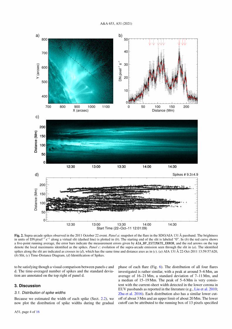
by AIA_BP_ESTIMATE_ERROR (shown as error bars). To identifythe major peaks but discard the wiggles, we first smoothed thebrightness profile along the slit by a five-point running average(shown as the red curve in (b)), and then located the local max-imums and minimums in a running box of 13 pixels. All localmaximums must exceed 20 DN pixel−1 s−1, an empirical back-ground set in this study. The distance between the two nearestlocal minimums found at each side of a spike is taken as itswidth (cf. Sect. 3.1). The identified major peaks are denoted byred arrows on the top of panel b.

Further, for the two disk events, #2 and #4, AIA 131 Åimages are co-registered to the first image taken during eachselected time interval using the SSW procedure DROT_MAP. Wemade the time-distance stack plot (panel c) by taking a slicealong the virtual slit from each image and then arranging theslices in chronological order. The temporal evolution of spikes

was then recorded in this time-distance diagram. We can seethat some spikes evolve consistently, some are wavering due toSADs, and others may apparently appear or disappear during theinvestigated time period. It is interesting that some SADs revealthemselves as dark, tadpole-like features in the time-distancediagram as they propagate through the slit (e.g., Fig. 2c). It canbe seen that SADs may not only flow along intra-spike chan-nels but also into the spikes, the latter of which may result in theapparent splitting of a spike (some clear examples can be seen inFig. 3c). Such interactions between bright spikes and dark down-flowing voids are suggested to be evidence for Rayleigh-Taylortype instabilities in the exhaust of reconnection jets (Guo et al.2014; Innes et al. 2014).

The identified spikes along the slit are plotted as crosses inpanel d, which has the same time and distance axes as the time-distance diagram in panel c. We find our identification algorithm

A51, page 3 of 16

A&A 653, A51 (2021)

700 800 900 1000 1100X (arcsec)

400

500

600

700

800Y

(ar

csec

)

0

b)

0 50 100 150 200Distance (Mm)

0

10

20

30

40

50

DN

pix

el−

1 s−

1

12:30 13:00 13:30 14:00 14:30

0

50

100

150

200

Dis

tanc

e (M

m)

c)

12:30 13:00 13:30 14:00 14:30

0

50

100

150

200

Dis

tanc

e (M

m)

d)

12:30 13:00 13:30 14:00 14:30Start Time (22−Oct−11 12:01:09)

0

50

100

150

200

Dis

tanc

e (M

m)

Spikes # 9.3±4.9

a)

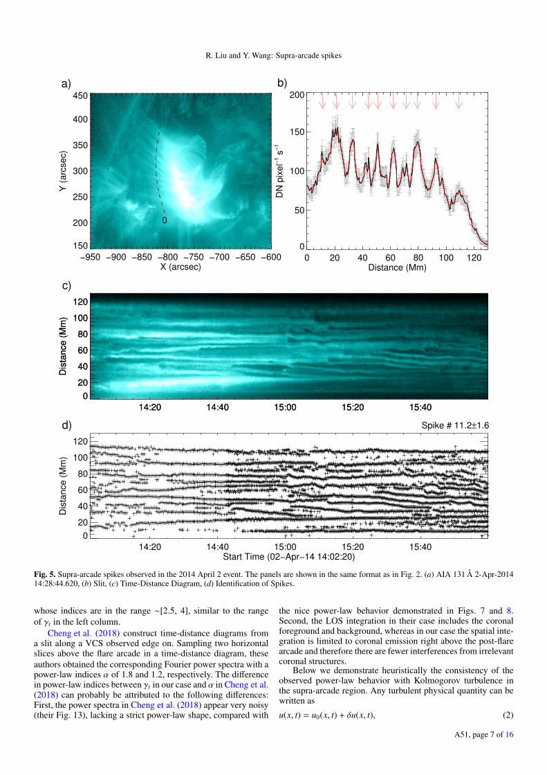
Fig. 2. Supra-arcade spikes observed in the 2011 October 22 event. Panel a: snapshot of the flare in the SDO/AIA 131 Å passband. The brightnessin units of DN pixel−1 s−1 along a virtual slit (dashed line) is plotted in (b). The starting end of the slit is labeled “0”. In (b) the red curve showsa five-point running average, the error bars indicate the measurement errors given by AIA_BP_ESTIMATE_ERROR, and the red arrows on the topdenote the local maximums identified as the spikes. Panel c: evolution of the supra-arcade emission seen through the slit in (a). The identifiedspikes along the slit are indicated as crosses in (d), which has the same time and distance axes as in (c). (a) AIA 131 Å 22-Oct-2011 13:59:57.620,(b) Slit, (c) Time-Distance Diagram, (d) Identification of Spikes.

to be satisfying though a visual comparison between panels c andd. The time-averaged number of spikes and the standard devia-tion are annotated on the top right of panel d.

3. Discussion

3.1. Distribution of spike widths

Because we estimated the width of each spike (Sect. 2.2), wenow plot the distribution of spike widths during the gradual

phase of each flare (Fig. 6). The distribution of all four flaresinvestigated is rather similar, with a peak at around 5–6 Mm, anaverage of 16–21 Mm, a standard deviation of 7–11 Mm, anda median of 15–19 Mm. The peak of 5–6 Mm is very consis-tent with the current-sheet width detected in the lower corona inEUV passbands as reported in the literature (e.g., Liu et al. 2010;Zhu et al. 2016). Each distribution also has a similar lower cut-off of about 3 Mm and an upper limit of about 20 Mm. The lowercutoff can be attributed to the running box of 13 pixels specified

A51, page 4 of 16

R. Liu and Y. Wang: Supra-arcade spikes

a)

−400 −300 −200 −100 0X (arcsec)

50

100

150

200

250

300

350

400

Y (

arcs

ec)

0

b)

0 50 100 150 200Distance (Mm)

0

20

40

60

80

DN

pix

el−

1 s−

1c)

07:40 08:00 08:20 08:40 09:00 09:20

0

50

100

150

200

Dis

tanc

e (M

m)

07:40 08:00 08:20 08:40 09:00 09:20

0

50

100

150

200

Dis

tanc

e (M

m)

d)

07:40 08:00 08:20 08:40 09:00 09:20Start Time (11−Apr−13 07:32:20)

0

50

100

150

200

Dis

tanc

e (M

m)

Spikes # 6.7±2.9

Fig. 3. Supra-arcade spikes observed in the 2013 April 11 event. The panels are shown in the same format as in Fig. 2. (a) AIA 131 Å 11-Apr-201307:53:56.620, (b) Slit, (c) Time-Distance Diagram, (d) Identification of Spikes.

in our algorithm, which effectively limits the spike width tobe above 6 pixels, or 2.6 Mm. This is smaller than the lowerlimit of the current-sheet width, 3 Mm, deduced by Guo et al.(2013) from the nonlinear scaling law of the plasmoid instabil-ity. We note that Lin et al. (2007, 2009) gave a larger lower limit(50 Mm) based on the linear scaling law.

Apparently, spike widths are log-normally, rather than nor-mally, distributed. In Fig. 6, employing a nonlinear least squaresfitting procedure MPFIT3 (Markwardt et al. 2009) and assuminga two-pixel measurement error, we fit each distribution with thefollowing function:

3 http://purl.com/net/mpfit

y(x) =C

xσ√

2πexp[−

(ln x − µ)2

2σ2

], (1)

where C is an arbitrary constant. The other two parameters (µ, σ)are annotated in the middle right of each panel. It is noteworthythat we obtain similar µ and σ in all four events.

3.2. Spatiotemporal structures of supra-arcadeEUV emission

We apply the Fourier transform to each vertical slice in the time-distance diagram in panel c of Figs. 2–5 to explore the struc-ture of the supra-arcade emission in terms of spatial frequency

A51, page 5 of 16

A&A 653, A51 (2021)

a)

850 900 950 1000 1050 1100X (arcsec)

−300

−250

−200

−150

−100

−50

Y (

arcs

ec)

0

b)

0 20 40 60 80 100 120Distance (Mm)

0

50

100

150

200

DN

pix

el−

1 s−

1

00:30 01:00 01:30 02:00

0

20

40

60

80

100

120

Dis

tanc

e (M

m)

c)

00:30 01:00 01:30 02:00

0

20

40

60

80

100

120

Dis

tanc

e (M

m)

d)

00:30 01:00 01:30 02:00Start Time (07−Nov−13 00:02:20)

0

20

40

60

80

100

120

Dis

tanc

e (M

m)

Spike # 7.9±2.2

Fig. 4. Supra-arcade spikes observed in the 2013 November 7 event. The panels are shown in the same format as in Fig. 2. (a) AIA 131 Å7-Nov-2013 00:25:44.620, (b) Slit, (c) Time-Distance Diagram, (d) Identification of Spikes.

k (Mm−1). We fit the Fourier power spectrum resulting from eachvertical slice with a power-law function and show the temporalvariation of the power-law index γs in the left column of Fig. 7.Collapsing the time-distance diagram along the time axis givesthe time-integrated EUV emission profile along the slit. Apply-ing the Fourier transform to this profile, we obtain power spectraexhibiting clear power-law behaviors (right column of Fig. 7),whose fitted indices are in the range ∼[4, 5], similar to the rangeof γs in the left column.

Similarly, we apply the Fourier transform to each horizon-tal slice in the time-distance diagram in panel c of Figs. 2–5 to

explore the structure of the supra-arcade emission in terms oftemporal frequency ν (mHz). Fitting the Fourier power spectrumfrom each horizontal slice by a power-law function, we show thevariation of the resultant power-law index γt along the virtual slitin the left column of Fig. 8. Collapsing the time-distance dia-gram along the distance axis, we effectively integrate the EUVemission along the slit, which emulates the situation when theVCS is observed edge on in the optically thin corona. This resultsin a time series of EUV emission sampled from a point on theVCS. The power spectra of spatially integrated EUV emissionalso exhibit clear power-law shapes (right column of Fig. 8),

A51, page 6 of 16

R. Liu and Y. Wang: Supra-arcade spikes

a)

−950 −900 −850 −800 −750 −700 −650 −600X (arcsec)

150

200

250

300

350

400

450

Y (

arcs

ec)

0

b)

0 20 40 60 80 100 120Distance (Mm)

0

50

100

150

200

DN

pix

el−

1 s−

1

c)

14:20 14:40 15:00 15:20 15:40

0

20

40

60

80

100

120

Dis

tanc

e (M

m)

14:20 14:40 15:00 15:20 15:40

0

20

40

60

80

100

120

Dis

tanc

e (M

m)

d)

14:20 14:40 15:00 15:20 15:40Start Time (02−Apr−14 14:02:20)

0

20

40

60

80

100

120

Dis

tanc

e (M

m)

Spike # 11.2±1.6

Fig. 5. Supra-arcade spikes observed in the 2014 April 2 event. The panels are shown in the same format as in Fig. 2. (a) AIA 131 Å 2-Apr-201414:28:44.620, (b) Slit, (c) Time-Distance Diagram, (d) Identification of Spikes.

whose indices are in the range ∼[2.5, 4], similar to the rangeof γt in the left column.

Cheng et al. (2018) construct time-distance diagrams froma slit along a VCS observed edge on. Sampling two horizontalslices above the flare arcade in a time-distance diagram, theseauthors obtained the corresponding Fourier power spectra with apower-law indices α of 1.8 and 1.2, respectively. The differencein power-law indices between γt in our case and α in Cheng et al.(2018) can probably be attributed to the following differences:First, the power spectra in Cheng et al. (2018) appear very noisy(their Fig. 13), lacking a strict power-law shape, compared with

the nice power-law behavior demonstrated in Figs. 7 and 8.Second, the LOS integration in their case includes the coronalforeground and background, whereas in our case the spatial inte-gration is limited to coronal emission right above the post-flarearcade and therefore there are fewer interferences from irrelevantcoronal structures.

Below we demonstrate heuristically the consistency of theobserved power-law behavior with Kolmogorov turbulence inthe supra-arcade region. Any turbulent physical quantity can bewritten as

u(x, t) = u0(x, t) + δu(x, t), (2)

A51, page 7 of 16

A&A 653, A51 (2021)

2011 OCT 22

0 5 10 15 20 25 30Spike Width (Mm)

0

500

1000

1500

2000

Spi

ke #

Peak = 5.2 MmMean = 16.5 Mm

Std = 7.2 MmMedian = 15.0 Mm

(1.77, 0.43)

2013 APR 11

0 10 20 30 40 50Spike Width (Mm)

0

200

400

600

Spi

ke #

Peak = 5.6 MmMean = 21.2 Mm

Std = 11.0 MmMedian = 19.0 Mm

(2.03, 0.51)

2013 NOV 06

0 5 10 15 20 25 30Spike Width (Mm)

0

200

400

600

800

1000

1200

Spi

ke #

Peak = 6.0 MmMean = 18.8 Mm

Std = 7.9 MmMedian = 17.0 Mm

(1.93, 0.44)

2014 APR 02

0 5 10 15 20 25Spike Width (Mm)

0

200

400

600

800

1000

1200

Spi

ke #

Peak = 5.6 MmMean = 18.3 Mm

Std = 7.5 MmMedian = 17.0 Mm

(1.89, 0.39)

Fig. 6. Distribution of the widths of SASs. Each panel shows the his-togram for one of the four events under investigation. The statistics ofthe distribution are indicated in the top right, and the fitting parame-ters (µ, σ) of the log-normal function (Eq. (1)) in the middle right. Thefitting function is plotted as a dashed curve.

12:30 13:00 13:30 14:00 14:30Start Time (22-Oct-11 12:01:09)

-6.0

-5.5

-5.0

-4.5

-4.0

-3.5

-3.0

γs

<γs> = -4.95 ± 0.29

0.1k (Mm-1)

10-15

10-10

10-5

100

105

Pow

er

γs = -4.71 ± 0.24

07:40 08:00 08:20 08:40 09:00 09:20Start Time (11-Apr-13 07:32:20)

-8

-7

-6

-5

-4

-3

γs

<γs> = -5.28 ± 0.61

0.1k (Mm-1)

10-8

10-6

10-4

10-2

100

102

104

Pow

er

γs = -4.51 ± 0.10

14:20 14:40 15:00 15:20 15:40Start Time (02-Apr-14 14:02:20)

-9

-8

-7

-6

-5

-4

-3

γs

<γs> = -5.09 ± 0.98

0.1k (Mm-1)

10-6

10-4

10-2

100

102

104

106

Pow

er

γs = -4.62 ± 0.18

18:00 18:20 18:40 19:00 19:20 19:40Start Time (18-Jun-15 17:42:20)

-6.0

-5.5

-5.0

-4.5

-4.0

-3.5

-3.0

γs

<γs> = -4.86 ± 0.32

0.1k (Mm-1)

10-8

10-6

10-4

10-2

100

102

104

Pow

er

γs = -4.35 ± 0.19

Fig. 7. Structure of supra-arcade EUV emission in terms of spatial fre-quency. The power spectrum of any vertical slice in the time-distancediagram (panel c of Figs. 2–5) is fitted with a power-law function. Thetemporal variation of the power-law index γs is shown in the left pan-els. The orange bars indicate the 1σ uncertainty estimates in the fittings.The power spectrum of the time-distance diagram collapsed along thetime axis is shown in the right panels.

where u0(x, t) varies smoothly at large spatiotemporal scales,while δu(x, t) fluctuates randomly at small scales, that is, thereis a large separation of space and time scales between the meanand fluctuating components. The two components hence respond

22−Oct−2011

0 50 100 150 200Distance (Mm)

−4

−3

−2

−1

0

1

γt

<γt> = −1.05 ± 0.61

22−Oct−2011

1 10ν (mHz)

10−14

10−12

10−10

10−8

10−6

10−4

10−2

Pow

er

γt = −2.37 ± 0.14

11−Apr−2013

0 50 100 150 200Distance (Mm)

−4

−3

−2

−1

0

1

γt

<γt> = −2.88 ± 0.70

11−Apr−2013

1 10ν (mHz)

10−6

10−4

10−2

100

102

104

Pow

er

γt = −3.41 ± 0.03

2−Apr−2014

0 20 40 60 80 100 120Distance (Mm)

−4

−3

−2

−1

0

1

γt

<γt> = −2.90 ± 0.44

2−Apr−2014

1 10ν (mHz)

10−6

10−4

10−2

100

102

104

Pow

er

γt = −3.74 ± 0.08

18−Jun−2015

0 50 100 150Distance (Mm)

−4

−3

−2

−1

0

1

γt

<γt> = −2.01 ± 0.85

18−Jun−2015

1 10ν (mHz)

10−6

10−4

10−2

100

102

104

Pow

er

γt = −3.49 ± 0.06

Fig. 8. Structure of supra-arcade EUV emission in terms of temporalfrequency. The power spectrum of any horizontal slice in the time-distance diagram (panel c of Figs. 2–5) is fitted with a power-law func-tion. The spatial variation of the power-law index γt along each slit(panel a in Figs. 2–5) is shown in the left panels. The orange bars indi-cate the 1σ uncertainty estimates in the fittings. The power spectrum ofthe time-distance diagram collapsed along the distance axis is shown inthe right panels.

distinctively to a long wavelength average, that is,

〈u0(x, t)〉 = u0(x, t) and 〈δu(x, t)〉 = 0. (3)

The Fourier transform of the observed intensity I = I0 + δIgives the power spectra

E(k) ∼ k−γs and E(ν) ∼ ν−γt , (4)

in terms of spatial frequency k and temporal frequency ν, respec-tively, as shown in Figs. 7 and 8. Here for clarity, the spec-tral index γs and γt are set as positive; I0 is transformed tothe low-frequency end of the power spectra; and δI to thehigher-frequency portion with power-law behavior, that is, δI2 ∼

E(k)k ∼ k−γs+1 ∼ l γs−1, which gives

δI ∼ l (γs−1)/2 ∼ l [3/2, 2], (5)

because γs is found to be in the range [4, 5]. Similarly, sinceδI2 ∼ E(ν)ν, we have

δI ∼ ν−(γt−1)/2 ∼ ν−[3/4, 3/2], (6)

with γt in the range [2.5, 4].On the other hand, the intensity of coronal emission lines

I ∼∫

n2ds (Aschwanden 2005, Sect. 2.8), where s is the distancealong the LOS. Expanding n according to Eq. (2), we have

I ∼∫

(n20 + 2n0δn + δn2) ds. (7)

The LOS integration a priori takes a long wavelength average,which gives

I0 ∼

∫n2

0 ds and δI ∼∫

δn2 ds. (8)

A51, page 8 of 16

R. Liu and Y. Wang: Supra-arcade spikes

As a comparison, we anticipate that the turbulent componentwould be smoothened out in white-light observations of theK-corona, in which the observed intensity is dominated byThomson scattering, that is, I ∼

∫nds.

The density perturbation δn is linked to the velocity fluctua-tion δu by the equation of continuation

∂δn∂t' −∇ · (n0δu), (9)

assuming that |δn| � n0 but |∂n0/∂t| � |∂δn/∂t| and u0 ' 0.Thus,

δn ∼ −n0

L0/t0δu ∼ −n0

δuVA, (10)

in orders of magnitude, where t0 and L0 are characteristic timeand length scale of the system, respectively. The assumption thatthe Alfvén speed VA is on the same order of magnitude as L0/t0implies that |δu| � VA. This is consistent with spectroscopicobservations of hot emission lines in the VCS, which give non-thermal velocities of no larger than 200 km s−1 (e.g., Li et al.2018). We further argue that the LOS integration from the side-on perspective of the VCS make relevant the size l of large eddiesin the flow velocity field u ' δu, where the thickness of theVCS is comparable to those of spikes; that is, δI ∼ δu2 l, wherel . L0. l can be deemed as the order of magnitude of distancesover which δu changes appreciably.

If the observed intensity perturbations δI result from a fullydeveloped turbulence following the famous universal law of Kol-mogorov and Obukhov (i.e., δu ∼ l1/3) (Landau & Lifshitz 1987,Sect. 33), then we have

δI ∼ l5/3. (11)

The index 5/3 falls nicely in the compact range [3/2, 2] as givenindependently by Eq. (5). With ν ∼ (l δu)−1 ∼ l−4/3, we have

δI ∼ ν−5/4, (12)

in which the index also falls in the compact range [3/4, 3/2] asgiven by Eq. (6).

Thus, when the fluctuations in coronal emission-line inten-sity observations are dominated by turbulence, the correspond-ing power spectra are expected to exhibit the power-law behavioras follows,

E(k) ∼ k−13/3 and E(ν) ∼ ν−7/2. (13)

As a further evidence of turbulence in the VCS region, we cansee from the left column of Fig. 8 that the power-law index γt isgenerally closer to the value of 7/2 in the middle of the slit, thatis, within the VCS region, than at the two ends of the slit, that is,outside of the VCS.

In contrast, the LOS integration from the edge-on perspectiveof the VCS gives δI ∼ δu2 L, where the depth of the VCS iscomparable to the axial length of the post-flare arcade (i.e., L �L0). This leads to power spectra in k−7/3 or ν−2, which are onlyslightly steeper than those obtained by Cheng et al. (2018).

3.3. Implication for ICMEs

Each SAS can be considered as a reconnection site on the 3DVCS in the wake of the CME. According to the standard model,each episode of magnetic reconnection of the overlying field atthe VCS adds a twist of roughly one turn to the burgeoning CME

flux rope. If magnetic reconnections at each SAS proceeds con-tinually, that is, there is no significant time interval between anytwo episodes of magnetic reconnection on the same SAS, then atany time we may assume that the number of ongoing reconnec-tion episodes roughly correspond to the number of SASs. Sincethe number of SASs is stable during the flare decay phase, weexpect that the outer shells of the flux rope are more or less uni-formly twisted (e.g., Wang et al. 2017). When the CME arrivesat the Earth, we would expect near-Earth spacecrafts to detect amagnetic cloud possessing magnetic twist of similar number ofturns in its outer shells as the number of SASs.

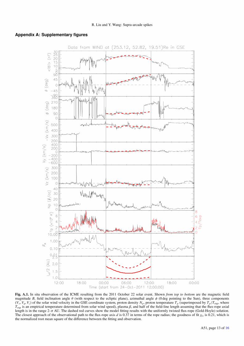
We fit the four ICMEs by a uniform-twist, force-freeflux rope model that takes into account the plasma motion(Wang et al. 2016). The in situ observations and correspondingfitting results are shown in Figs. A.1–A.4. The model yieldsthe twist density τ = rBφ/Bz in local cylindrical coordinates(r, φ, z) with the z-axis directed along the flux-rope axis. Theτ is given in units of the number of field line turns per unitAU along the flux-rope axis. The helicity (twist) signs are neg-ative for all four events, which, except Event #3, originate fromthe northern hemisphere, which is consistent with the cycle-independent dominance of negative helicity in the same hemi-sphere (Zhou et al. 2020, and references therein). Event #3 orig-inates from a decayed active region (AR 11882) in the south-ern hemisphere close to the equator. When it is located near thedisk center, the active region exhibits a weak reverse-S geom-etry manifested by coronal loops in EUV (Fig. 9c), associatedwith a filament aligned along the polarity inversion line witha similar geometry, signaling the presence of negative helicity.In contrast, AR 11314, the source region of Event #1 exhibitsa forward-S geometry in the east and a reverse-S geometry inthe west (Fig. 9a), suggesting that the CME probably originatesfrom the west side of the active region. The other two sourceregions, ARs 11719 (Fig. 9b) and 12027 (Fig. 9d), are clearlyreverse-S shaped; the latter is outlined by a sigmoidal filament.Additionally, different aspects of the source region of Event#2, AR 11719, has been studied in detail by several authors(Vemareddy & Mishra 2015; Vemareddy et al. 2016; Guo et al.2019).

The axial length of the ICME is unknown but assumed tobe lie in the range 2–πAU. At the lower end, the flux ropeis so stretched that it is “folded” in half between the Sun andEarth; but at the higher end, the rope is circular (Wang et al.2015). Alternatively, Hu et al. (2015) compared the lengths ofICME field lines that are derived from energetic electron burstsobserved at 1 AU and the magnetic twist derived from the Grad-Shafranov reconstruction method. These authors concluded thatthe effective axial lengths of the selected ICME events rangebetween 2 AU and 4 AU. Unfortunately none of our selectedevents is associated with in situ energetic electron bursts. How-ever, the comparison between the number of SASs and the mag-netic twist of ICMEs as below may shed new light onto theiraxial lengths.

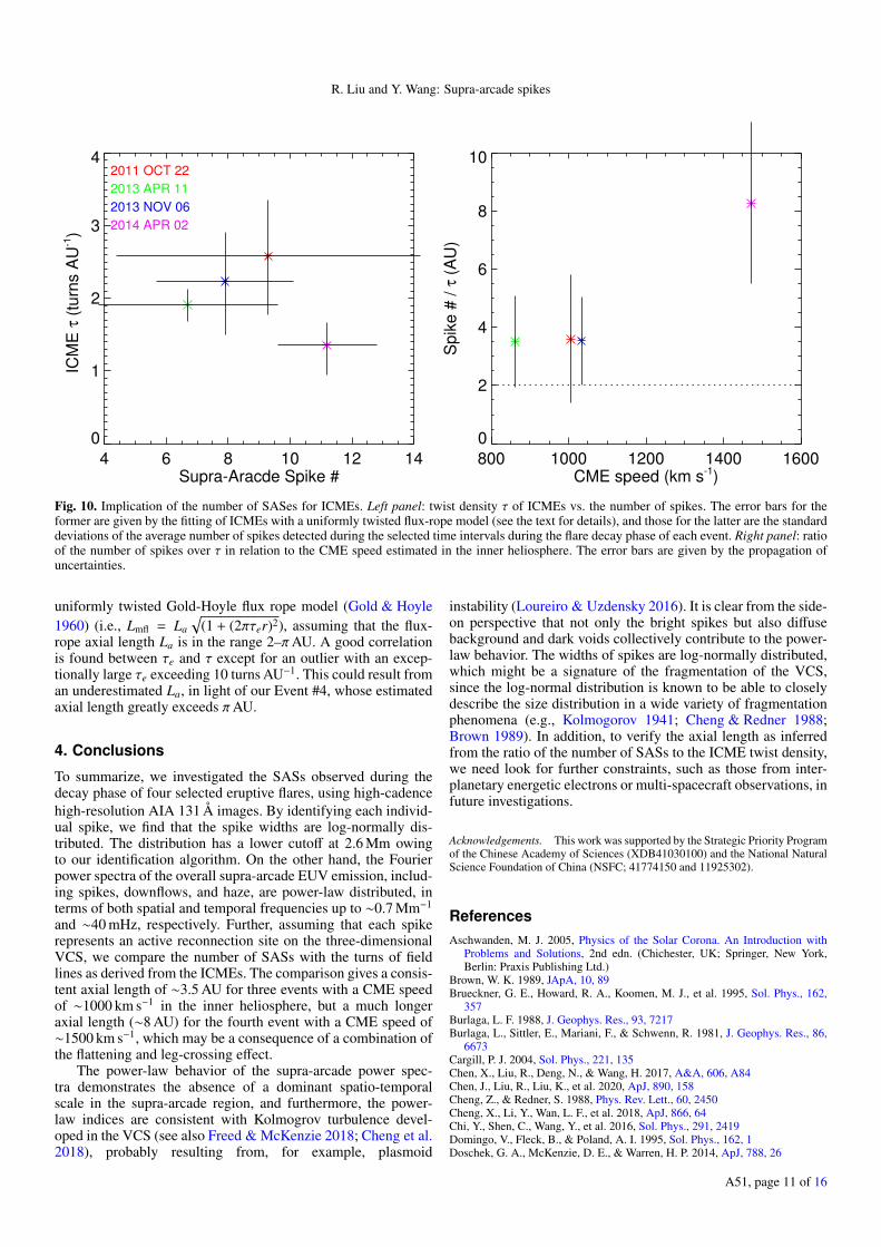
In the first three events, we found that τ linearly increaseswith the increasing number of SASs (left panel of Fig. 10). Fur-ther, the ratio of the number of SASs to τ gives a similar length ofthe flux-rope axis(i.e., ∼3.5 AU; middle panel of Fig. 10), whichis slightly above πAU, but still falls in the range suggested byHu et al. (2015). However, the fourth event seem to be an out-lier: this is the only event originating from close to the east limb(about 60◦ east), but the resultant ICME is still “skimmed” bythe near-Earth spacecraft for over 30 h (Fig. A.4), indicating itslarge size; the ICME has a moderate τ but the number of SASsis the largest among the four events, which is translated to an

A51, page 9 of 16

A&A 653, A51 (2021)

a)

−100 0 100 200 300 400

200

300

400

500

600

700

Y (

arcs

ec)

AR 11314

b)

−400 −350 −300 −250 −200 −150 −100 −50

50

100

150

200

250

300

350

400

AR 11719

c)

100 200 300 400 500X (arcsec)

−400

−300

−200

−100

Y (

arcs

ec)

AR 11882

d)

−900 −850 −800 −750 −700 −650 −600X (arcsec)

150

200

250

300

350

400

AR 12027

Fig. 9. Four active regions under investigation as observed by SDO/AIA. (a) AIA 193 Å 2011-10-16T21:30:43, (b) AIA 94 Å 2013-04-11T06:00:37, (c) AIA 193 Å 2013-10-31T22:00:42, (d) AIA 193 Å 2014-04-02T13:00:42.

axial length of 8.3 AU. These may be caused by two differentbut interrelated effects, both resulting from its exceptionally fastspeed (∼1500 km s−1 projected on the plane of sky) as measuredin the inner heliosphere by SOHO/LASCO.

First, the ICME experiences a much stronger resistance thanthe other three events when it “plows” through the solar wind,since in principle the aerodynamic drag force applied on theICME is proportional to the square of the difference betweenthe ICME speed and the solar wind speed (Cargill 2004). Hencethe drag force acting on the fourth ICME is roughly 3.5 times morethan that on the other three, given the solar wind speed in the range400–450 km s−1. The resistance restricts the ICME radial muchmore than its lateral expansion (e.g., Manchester et al. 2004).However, this would lead to an unrealistically highly flattenedshape (right panel of Fig. 10) if the spacecraft crossed the nose

of the flux rope. We then suggest that the spacecraft actually tra-verses the leg of the ICME, which is evidenced by its axis beingoriented almost along the Sun-Earth line (Table 1). As a compari-son, the flux-rope axes in the other three events make large angleswith respect to the Sun-Earth line. Hence at the time of the space-craft passing, the nose of the fourth ICME is significantly past theEarth, resulting in an axial length much longer than πAU. How-ever, if the axis has a circular shape, the nose of the ICME would beover 2.5 AU from the Sun. This is translated to an average propa-gation speed of∼1300 km s−1, which is also unrealistic. In reality,we may be witnessing a combination of both the flattening and theleg-passing effect.

Wang et al. (2016) converted the field-line length Lmfl esti-mated by the electron-probe method in seven magnetic cloudsfrom Kahler et al. (2011) to a twist density τe based on the

A51, page 10 of 16

R. Liu and Y. Wang: Supra-arcade spikes

4 6 8 10 12 14Supra-Aracde Spike #

0

1

2

3

4

ICM

E τ

(tu

rns

AU

-1)

2011 OCT 222013 APR 112013 NOV 062014 APR 02

800 1000 1200 1400 1600CME speed (km s-1)

0

2

4

6

8

10

Spi

ke #

/ τ (

AU

)

Fig. 10. Implication of the number of SASes for ICMEs. Left panel: twist density τ of ICMEs vs. the number of spikes. The error bars for theformer are given by the fitting of ICMEs with a uniformly twisted flux-rope model (see the text for details), and those for the latter are the standarddeviations of the average number of spikes detected during the selected time intervals during the flare decay phase of each event. Right panel: ratioof the number of spikes over τ in relation to the CME speed estimated in the inner heliosphere. The error bars are given by the propagation ofuncertainties.

uniformly twisted Gold-Hoyle flux rope model (Gold & Hoyle1960) (i.e., Lmfl = La

√(1 + (2πτer)2), assuming that the flux-

rope axial length La is in the range 2–πAU. A good correlationis found between τe and τ except for an outlier with an excep-tionally large τe exceeding 10 turns AU−1. This could result froman underestimated La, in light of our Event #4, whose estimatedaxial length greatly exceeds πAU.

4. Conclusions

To summarize, we investigated the SASs observed during thedecay phase of four selected eruptive flares, using high-cadencehigh-resolution AIA 131 Å images. By identifying each individ-ual spike, we find that the spike widths are log-normally dis-tributed. The distribution has a lower cutoff at 2.6 Mm owingto our identification algorithm. On the other hand, the Fourierpower spectra of the overall supra-arcade EUV emission, includ-ing spikes, downflows, and haze, are power-law distributed, interms of both spatial and temporal frequencies up to ∼0.7 Mm−1

and ∼40 mHz, respectively. Further, assuming that each spikerepresents an active reconnection site on the three-dimensionalVCS, we compare the number of SASs with the turns of fieldlines as derived from the ICMEs. The comparison gives a consis-tent axial length of ∼3.5 AU for three events with a CME speedof ∼1000 km s−1 in the inner heliosphere, but a much longeraxial length (∼8 AU) for the fourth event with a CME speed of∼1500 km s−1, which may be a consequence of a combination ofthe flattening and leg-crossing effect.

The power-law behavior of the supra-arcade power spec-tra demonstrates the absence of a dominant spatio-temporalscale in the supra-arcade region, and furthermore, the power-law indices are consistent with Kolmogrov turbulence devel-oped in the VCS (see also Freed & McKenzie 2018; Cheng et al.2018), probably resulting from, for example, plasmoid

instability (Loureiro & Uzdensky 2016). It is clear from the side-on perspective that not only the bright spikes but also diffusebackground and dark voids collectively contribute to the power-law behavior. The widths of spikes are log-normally distributed,which might be a signature of the fragmentation of the VCS,since the log-normal distribution is known to be able to closelydescribe the size distribution in a wide variety of fragmentationphenomena (e.g., Kolmogorov 1941; Cheng & Redner 1988;Brown 1989). In addition, to verify the axial length as inferredfrom the ratio of the number of SASs to the ICME twist density,we need look for further constraints, such as those from inter-planetary energetic electrons or multi-spacecraft observations, infuture investigations.

Acknowledgements. This work was supported by the Strategic Priority Programof the Chinese Academy of Sciences (XDB41030100) and the National NaturalScience Foundation of China (NSFC; 41774150 and 11925302).

ReferencesAschwanden, M. J. 2005, Physics of the Solar Corona. An Introduction with

Problems and Solutions, 2nd edn. (Chichester, UK; Springer, New York,Berlin: Praxis Publishing Ltd.)

Brown, W. K. 1989, JApA, 10, 89Brueckner, G. E., Howard, R. A., Koomen, M. J., et al. 1995, Sol. Phys., 162,

357Burlaga, L. F. 1988, J. Geophys. Res., 93, 7217Burlaga, L., Sittler, E., Mariani, F., & Schwenn, R. 1981, J. Geophys. Res., 86,

6673Cargill, P. J. 2004, Sol. Phys., 221, 135Chen, X., Liu, R., Deng, N., & Wang, H. 2017, A&A, 606, A84Chen, J., Liu, R., Liu, K., et al. 2020, ApJ, 890, 158Cheng, Z., & Redner, S. 1988, Phys. Rev. Lett., 60, 2450Cheng, X., Li, Y., Wan, L. F., et al. 2018, ApJ, 866, 64Chi, Y., Shen, C., Wang, Y., et al. 2016, Sol. Phys., 291, 2419Domingo, V., Fleck, B., & Poland, A. I. 1995, Sol. Phys., 162, 1Doschek, G. A., McKenzie, D. E., & Warren, H. P. 2014, ApJ, 788, 26

A51, page 11 of 16

A&A 653, A51 (2021)

Freed, M. S., & McKenzie, D. E. 2018, ApJ, 866, 29Gold, T., & Hoyle, F. 1960, MNRAS, 120, 89Gou, T., Liu, R., & Wang, Y. 2015, Sol. Phys., 290, 2211Gou, T., Liu, R., Kliem, B., Wang, Y., & Veronig, A. M. 2019, Sci. Adv., 5, 7004Guo, L.-J., Bhattacharjee, A., & Huang, Y.-M. 2013, ApJ, 771, L14Guo, L. J., Huang, Y. M., Bhattacharjee, A., & Innes, D. E. 2014, ApJ, 796,

L29Guo, J., Wang, H., Wang, J., et al. 2019, ApJ, 874, 181Hanneman, W. J., & Reeves, K. K. 2014, ApJ, 786, 95Hu, Q., Qiu, J., & Krucker, S. 2015, J. Geophys. Res. (Space Phys.), 120, 5266Innes, D. E., Guo, L. J., Bhattacharjee, A., Huang, Y. M., & Schmit, D. 2014,

ApJ, 796, 27Janvier, M., Aulanier, G., & Démoulin, P. 2015, Sol. Phys., 290, 3425Jing, J., Xu, Y., Cao, W., et al. 2016, Sci. Rep., 6, 24319Kahler, S. W., Krucker, S., & Szabo, A. 2011, J. Geophys. Res. (Space Phys.),

116, A01104Kolmogorov, A. N. 1941, in Dokl Akad. Nauk. SSSR, 99Kopp, R. A., & Pneuman, G. W. 1976, Sol. Phys., 50, 85Landau, L. D., & Lifshitz, E. M. 1987, Fluid Mechanics, 2nd edn. (Butterworth-

Heinemann publications)Lemen, J. R., Title, A. M., Akin, D. J., et al. 2012, Sol. Phys., 275, 17Li, T., & Zhang, J. 2015, ApJ, 804, L8Li, Y., Xue, J. C., Ding, M. D., et al. 2018, ApJ, 853, L15Lin, J., & Forbes, T. G. 2000, J. Geophys. Res., 105, 2375Lin, J., Raymond, J. C., & van Ballegooijen, A. A. 2004, ApJ, 602, 422Lin, J., Ko, Y. K., Sui, L., et al. 2005, ApJ, 622, 1251Lin, J., Li, J., Forbes, T. G., et al. 2007, ApJ, 658, L123Lin, J., Li, J., Ko, Y.-K., & Raymond, J. C. 2009, ApJ, 693, 1666Lin, J., Murphy, N. A., Shen, C., et al. 2015, Space Sci. Rev., 194, 237Liu, R. 2013, MNRAS, 434, 1309Liu, R. 2020, Res. Astron. Astrophys., 20, 165Liu, R., Lee, J., Wang, T., et al. 2010, ApJ, 723, L28Liu, R., Wang, T.-J., Lee, J., et al. 2011, Res. Astron. Astrophys., 11, 1209Liu, W., Chen, Q., & Petrosian, V. 2013, ApJ, 767, 168Liu, R., Chen, J., Wang, Y., & Liu, K. 2016, Sci. Rep., 6, 34021Lörincík, J., Aulanier, G., Dudík, J., Zemanová, A., & Dzifcáková, E. 2019, ApJ,

881, 68Loureiro, N. F., & Uzdensky, D. A. 2016, Plasma Phys. Control. Fusion, 58

Manchester, W. B., Gombosi, T. I., Roussev, I., et al. 2004, J. Geophys. Res.(Space Phys.), 109, A02107

Markwardt, C. B. 2009, in Astronomical Data Analysis Software and SystemsXVIII, eds. D. A. Bohlender, D. Durand, & P. Dowler, ASP Conf. Ser., 411,251

McKenzie, D. E. 2013, ApJ, 766, 39McKenzie, D. E., & Hudson, H. S. 1999, ApJ, 519, L93O’Dwyer, B., Del Zanna, G., Mason, H. E., Weber, M. A., & Tripathi, D. 2010,

A&A, 521, A21Pesnell, W. D., Thompson, B. J., & Chamberlin, P. C. 2012, Sol. Phys., 275, 3Qiu, Y., Guo, Y., Ding, M., & Zhong, Z. 2020, ApJ, 901, 13Reeves, K. K., Freed, M. S., McKenzie, D. E., & Savage, S. L. 2017, ApJ, 836,

55Samanta, T., Tian, H., Chen, B., et al. 2021, The Innovation, 2Savage, S. L., McKenzie, D. E., Reeves, K. K., Forbes, T. G., & Longcope,

D. W. 2010, ApJ, 722, 329Savage, S. L., Holman, G., Reeves, K. K., et al. 2012a, ApJ, 754, 13Savage, S. L., McKenzie, D. E., & Reeves, K. K. 2012b, ApJ, 747, L40Scott, R. B., McKenzie, D. E., & Longcope, D. W. 2016, ApJ, 819, 56Shibata, K., Masuda, S., Shimojo, M., et al. 1995, ApJ, 451, L83Švestka, Z., Fárník, F., Hudson, H. S., & Hick, P. 1998, Sol. Phys., 182, 179Titov, V. S., Hornig, G., & Démoulin, P. 2002, J. Geophys. Res. (Space Phys.),

107, 1164Vemareddy, P., & Mishra, W. 2015, ApJ, 814, 59Vemareddy, P., Möstl, C., Amerstorfer, T., et al. 2016, ApJ, 828, 12Wang, H., & Liu, C. 2012, ApJ, 760, 101Wang, Y., Zhou, Z., Shen, C., Liu, R., & Wang, S. 2015, J. Geophys. Res. (Space

Phys.), 120, 1543Wang, Y., Zhuang, B., Hu, Q., et al. 2016, J. Geophys. Res. (Space Phys.), 121,

9316Wang, W., Liu, R., Wang, Y., et al. 2017, Nat. Commun., 8, 1330Warren, H. P., O’Brien, C. M., & Sheeley, N. R., Jr. 2011, ApJ, 742, 92Warren, H. P., Brooks, D. H., Ugarte-Urra, I., et al. 2018, ApJ, 854, 122Webb, D. F., Burkepile, J., Forbes, T. G., & Riley, P. 2003, J. Geophys. Res.

(Space Phys.), 108, 1440Xue, J., Su, Y., Li, H., & Zhao, X. 2020, ApJ, 898, 88Zhou, Z., Liu, R., Cheng, X., et al. 2020, ApJ, 891, 180Zhu, C., Liu, R., Alexander, D., & McAteer, R. T. J. 2016, ApJ, 821, L29

A51, page 12 of 16

R. Liu and Y. Wang: Supra-arcade spikes

Appendix A: Supplementary figures

Fig. A.1. In situ observation of the ICME resulting from the 2011 October 22 solar event. Shown from top to bottom are the magnetic fieldmagnitude B, field inclination angle θ (with respect to the ecliptic plane), azimuthal angle φ (0 deg pointing to the Sun), three components(Vx,Vy,Vz) of the solar wind velocity in the GSE coordinate system, proton density Np, proton temperature Tp (superimposed by Tp/Texp, whereTexp is an empirical temperature determined from solar wind speed), plasma β, and half of the field-line length assuming that the flux-rope axiallength is in the range 2–π AU. The dashed red curves show the model fitting results with the uniformly twisted flux-rope (Gold-Hoyle) solution.The closest approach of the observational path to the flux-rope axis d is 0.37 in terms of the rope radius; the goodness of fit χn is 0.21, which isthe normalized root mean square of the difference between the fitting and observation.

A51, page 13 of 16

A&A 653, A51 (2021)

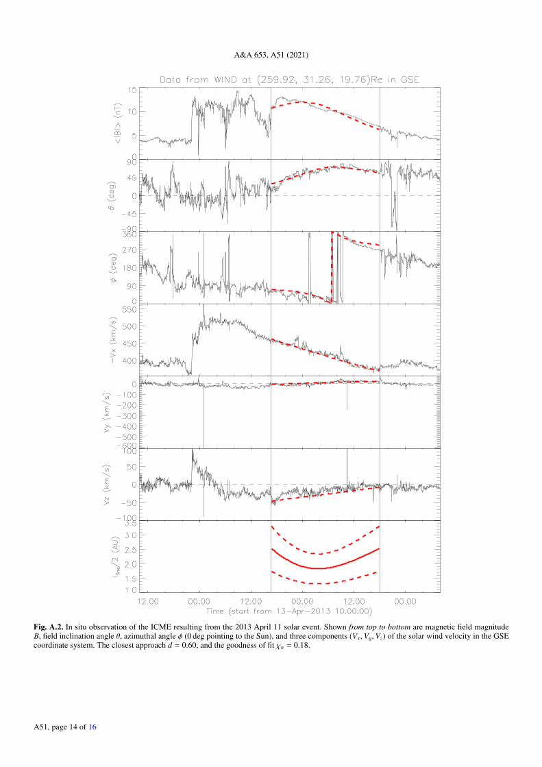
Fig. A.2. In situ observation of the ICME resulting from the 2013 April 11 solar event. Shown from top to bottom are magnetic field magnitudeB, field inclination angle θ, azimuthal angle φ (0 deg pointing to the Sun), and three components (Vx,Vy,Vz) of the solar wind velocity in the GSEcoordinate system. The closest approach d = 0.60, and the goodness of fit χn = 0.18.

A51, page 14 of 16

R. Liu and Y. Wang: Supra-arcade spikes

Fig. A.3. In situ observation of the ICME resulting from the 2013 November 7 solar event. The panels are shown in the same format as in Fig. A.2.The closest approach d = 0.23, and the goodness of fit χn = 0.19.

A51, page 15 of 16

A&A 653, A51 (2021)

Fig. A.4. In situ observation of the ICME resulting from the 2014 April 2 solar event. The panels are shown in the same format as in Fig. A.2. Theclosest approach d = 0.88, and the goodness of fit χn = 0.33.

A51, page 16 of 16