investigation of thermoacoustic performance of...
TRANSCRIPT

INVESTIGATION OF THERMOACOUSTIC
PERFORMANCE OF STANDING AND
TRAVELING WAVE THERMOACOUSTIC
ENGINES
by
Konstantin N. Tourkov
B.S. in Mechanical Engineering, University of Pittsburgh, 2011
Submitted to the Graduate Faculty of
the Swanson School of Engineering in partial fulfillment
of the requirements for the degree of
Master of Science in Mechanical Engineering
University of Pittsburgh
2013
UNIVERSITY OF PITTSBURGH
SWANSON SCHOOL OF ENGINEERING
This thesis was presented
by
Konstantin N. Tourkov
It was defended on
March 26, 2013
and approved by
Laura A. Schaefer, Ph.D., Associate Professor,
Department of Mechanical Engineering and Materials Science
Jeffrey S. Vipperman, Ph.D., Associate Professor,
Department of Mechanical Engineering and Materials Science
Mark Kimber, Ph.D., Assistant Professor,
Department of Mechanical Engineering and Materials Science
Thesis Advisor: Laura A. Schaefer, Ph.D., Associate Professor,
Department of Mechanical Engineering and Materials Science
ii
INVESTIGATION OF THERMOACOUSTIC PERFORMANCE OF
STANDING AND TRAVELING WAVE THERMOACOUSTIC ENGINES
Konstantin N. Tourkov, M.S.
University of Pittsburgh, 2013
A standing wave thermoacoustic engine was designed and constructed to examine the effect
of curvature on thermoacoustic performance. Sound pressure level at the pressure node of
the engine was recorded in conjuction with the temperature at the hot and ambient sides
of the stack. Curvature was varied using flexible tubing from 0 to 45. It was found
that the curvature had a negative effect on the thermoacoustic intensity, measured using
the sound pressure level and the temperature difference between the hot and ambient sides
of the stack. Additionally, a strong relationship between the sound pressure level and the
temperature behavior was identified. The findings of the investigation were applied to a
study of a traveling wave engine. A looped tube design was employed with a regenerator
mounted in a straight section of the tube. Thermocouples were mounted in the regenerator
to investigate the temperature behavior. Initial results of the thermoacoustic effect were
established by calculating the difference in behavior between operation with oscillation and
without. These were followed by an investigation of the relationship between the temperature
behavior and the positioning of the regenerator in the looped tube. An optimal spacing was
identified for positioning the stack in the straight portion of the tube.
iii
TABLE OF CONTENTS
1.0 INTRODUCTION . . . . . . . . . . . . . . . . . . . . . . . . . . . . . . . . . 1
1.1 Brief History . . . . . . . . . . . . . . . . . . . . . . . . . . . . . . . . . . . 1
1.2 Thermoacoustic Engines: Standing Wave and Traveling Wave . . . . . . . . 2
1.2.1 Standing Wave Engines . . . . . . . . . . . . . . . . . . . . . . . . . . 3
1.2.2 Traveling Wave Engines . . . . . . . . . . . . . . . . . . . . . . . . . . 4
1.3 Motivation for Thermoacoustic Refrigeration . . . . . . . . . . . . . . . . . 8
1.3.1 Absorption Cycles . . . . . . . . . . . . . . . . . . . . . . . . . . . . . 8
1.3.2 Vapor Compression . . . . . . . . . . . . . . . . . . . . . . . . . . . . 10
1.3.3 Thermoacoustic Cooling . . . . . . . . . . . . . . . . . . . . . . . . . 11
1.4 Goals of This Work . . . . . . . . . . . . . . . . . . . . . . . . . . . . . . . . 12
2.0 THERMOACOUSTIC THEORY . . . . . . . . . . . . . . . . . . . . . . . . 13
2.1 Linear Acoustic Theory . . . . . . . . . . . . . . . . . . . . . . . . . . . . . 13
2.2 Streaming Losses . . . . . . . . . . . . . . . . . . . . . . . . . . . . . . . . . 16
2.2.1 Gedeon Streaming . . . . . . . . . . . . . . . . . . . . . . . . . . . . . 16
2.2.2 Rayleigh Streaming . . . . . . . . . . . . . . . . . . . . . . . . . . . . 18
2.3 Acoustic Losses . . . . . . . . . . . . . . . . . . . . . . . . . . . . . . . . . . 20
2.4 Viscous Losses . . . . . . . . . . . . . . . . . . . . . . . . . . . . . . . . . . 21
2.5 Thermal Losses . . . . . . . . . . . . . . . . . . . . . . . . . . . . . . . . . . 22
3.0 STANDING WAVE INVESTIGATION . . . . . . . . . . . . . . . . . . . . 26
3.1 Design and Construction . . . . . . . . . . . . . . . . . . . . . . . . . . . . . 26
3.1.1 Stack Length and Position . . . . . . . . . . . . . . . . . . . . . . . . 26
3.1.2 Pore Geometry and Size . . . . . . . . . . . . . . . . . . . . . . . . . . 27
iv

3.1.3 Resonator . . . . . . . . . . . . . . . . . . . . . . . . . . . . . . . . . 27
3.1.4 Data Acquisition . . . . . . . . . . . . . . . . . . . . . . . . . . . . . . 28
3.2 Results: Temperature Behavior . . . . . . . . . . . . . . . . . . . . . . . . . 30
3.2.1 Hot Side Behavior . . . . . . . . . . . . . . . . . . . . . . . . . . . . . 30
3.2.2 Ambient Side Behavior . . . . . . . . . . . . . . . . . . . . . . . . . . 33
3.2.3 Trends Between Temperature and Curvature . . . . . . . . . . . . . . 34
3.3 Results: Acoustic Behavior . . . . . . . . . . . . . . . . . . . . . . . . . . . 36
3.3.1 General Oscillation Behavior . . . . . . . . . . . . . . . . . . . . . . . 36
3.3.2 Trends Between SPL and Curvature . . . . . . . . . . . . . . . . . . . 36
4.0 TRAVELING WAVE INVESTIGATION . . . . . . . . . . . . . . . . . . . 40
4.1 Design and Construction . . . . . . . . . . . . . . . . . . . . . . . . . . . . . 40
4.1.1 Resonator . . . . . . . . . . . . . . . . . . . . . . . . . . . . . . . . . 40
4.1.2 Regenerator . . . . . . . . . . . . . . . . . . . . . . . . . . . . . . . . 41
4.2 Experimental Setup . . . . . . . . . . . . . . . . . . . . . . . . . . . . . . . 43
4.3 Results: Stack Positioning Effects on Thermoacoustic Behavior . . . . . . . 45
4.3.1 Patterns In Thermoacoustic Behavior . . . . . . . . . . . . . . . . . . 45
4.3.2 Ambient Side Behavior . . . . . . . . . . . . . . . . . . . . . . . . . . 48
4.3.3 Hot Side Behavior . . . . . . . . . . . . . . . . . . . . . . . . . . . . . 48
4.3.4 Stack Placement and Intensity of The Thermoacoustic Effect . . . . . 49
4.4 Discussion . . . . . . . . . . . . . . . . . . . . . . . . . . . . . . . . . . . . . 51
5.0 CONCLUSIONS AND FURTHER RECOMMENDATIONS . . . . . . 53
5.1 Conclusions . . . . . . . . . . . . . . . . . . . . . . . . . . . . . . . . . . . . 53
5.2 Future Work . . . . . . . . . . . . . . . . . . . . . . . . . . . . . . . . . . . 54
BIBLIOGRAPHY . . . . . . . . . . . . . . . . . . . . . . . . . . . . . . . . . . . . 55
v

LIST OF FIGURES
1 Quarter-wave standing wave TAE [11] . . . . . . . . . . . . . . . . . . . . . . 3
2 Standing wave TAE cycle . . . . . . . . . . . . . . . . . . . . . . . . . . . . . 5
3 Standing wave TAE P-V diagram corresponding to cycle shown in Figure 2. . 5
4 Various traveling wave engine designs [18] . . . . . . . . . . . . . . . . . . . . 6
5 Diagram of a traveling wave cycle . . . . . . . . . . . . . . . . . . . . . . . . 7
6 Traveling wave TAE P-V diagram corresponding to cycle in Figure 5 [18]. . . 8
7 Diagram of a typical absorption cycle . . . . . . . . . . . . . . . . . . . . . . 9
8 Diagram of a typical VC cycle . . . . . . . . . . . . . . . . . . . . . . . . . . 10
9 Illustration of net mass flow occurence in pulse tube [33]. . . . . . . . . . . . 18
10 Mass flux profile in pulse tubes from central axis to wall [33]. . . . . . . . . . 18
11 Image of streaming taken using Doppler velocimetry [38]. . . . . . . . . . . . 19
12 Velocity filed observed using LDA and BSA [39]. . . . . . . . . . . . . . . . . 19
13 Relation between axial acoustic and axial streaming velocities [39]. . . . . . . 19
14 Real and imaginary parts of F (λ) for various pore geometries [28]. . . . . . . 20
15 Experimental results compared to analytical forms for heat compared to the
tempertaure difference [40]. . . . . . . . . . . . . . . . . . . . . . . . . . . . . 21
16 TAR design [45] . . . . . . . . . . . . . . . . . . . . . . . . . . . . . . . . . . 23
17 Thermoacoustic refrigerator thermal and viscous losses [45]. . . . . . . . . . . 23
18 TAR hot side exchanger thermal and viscous losses [45]. . . . . . . . . . . . . 24
19 TAR hot side exchanger thermal and viscous losses [32]. . . . . . . . . . . . . 24
20 Convective losses [32] . . . . . . . . . . . . . . . . . . . . . . . . . . . . . . . 25
21 Radiation losses [32] . . . . . . . . . . . . . . . . . . . . . . . . . . . . . . . . 25
vi
22 Diagram of standing wave device used in testing . . . . . . . . . . . . . . . . 28
23 Diagram of hot side of stack assembly . . . . . . . . . . . . . . . . . . . . . . 29
24 Initial response of SWTAE to 5V input . . . . . . . . . . . . . . . . . . . . . 30
25 Hot and ambient side temperature and SPL results for each of 3 runs for all
curvatures . . . . . . . . . . . . . . . . . . . . . . . . . . . . . . . . . . . . . 31
26 Hot side average histogram for each curvature. . . . . . . . . . . . . . . . . . 32
27 Hot side averages for each curvature . . . . . . . . . . . . . . . . . . . . . . . 32
28 Ambient side average histogram for each curvature. . . . . . . . . . . . . . . . 33
29 Ambient side averages for each curvature . . . . . . . . . . . . . . . . . . . . 34
30 Hot side overall averages with linear regression prediction. . . . . . . . . . . . 35
31 Ambient side overall averages. . . . . . . . . . . . . . . . . . . . . . . . . . . 35
32 Sound Pressure Histogram . . . . . . . . . . . . . . . . . . . . . . . . . . . . 37
33 Average SPL for each curvature. . . . . . . . . . . . . . . . . . . . . . . . . . 38
34 Average SPL with regression analysis. . . . . . . . . . . . . . . . . . . . . . . 38
35 Sound Pressure vs. Temperature Difference . . . . . . . . . . . . . . . . . . . 39
36 Picture of traveling wave TAE . . . . . . . . . . . . . . . . . . . . . . . . . . 42
37 Housing design used to insure air tightness. . . . . . . . . . . . . . . . . . . . 42
38 Regenerator used in the construction of the TAE. . . . . . . . . . . . . . . . . 42
39 Ambient side thermocouple positioning . . . . . . . . . . . . . . . . . . . . . 44
40 Regenerator position diagram . . . . . . . . . . . . . . . . . . . . . . . . . . . 44
41 Hot side individual runs. . . . . . . . . . . . . . . . . . . . . . . . . . . . . . 46
42 Ambient side individual runs. . . . . . . . . . . . . . . . . . . . . . . . . . . . 46
43 Hot side thermocouple readings. . . . . . . . . . . . . . . . . . . . . . . . . . 46
44 Ambient side thermocouple readings. . . . . . . . . . . . . . . . . . . . . . . . 46
45 Hot side temperature difference . . . . . . . . . . . . . . . . . . . . . . . . . . 47
46 Variation in hot side calculation. . . . . . . . . . . . . . . . . . . . . . . . . . 47
47 Percent error with respect to lower hot side average . . . . . . . . . . . . . . 47
48 Ambient side averaged oscillation and no oscillation runs. . . . . . . . . . . . 48
49 Ambient side temperature difference between run averages. . . . . . . . . . . 48
50 Hot side averaged oscillation and no oscillation runs. . . . . . . . . . . . . . . 49
vii

51 Hot side temperature difference between run averages. . . . . . . . . . . . . . 49
52 Normalized ambient temperature difference. . . . . . . . . . . . . . . . . . . . 50
53 Normalized hot temperature difference. . . . . . . . . . . . . . . . . . . . . . 50
54 Ambient side stack temperature vs. stack positioning. . . . . . . . . . . . . . 51
55 Hot side stack temperature vs. stack positioning. . . . . . . . . . . . . . . . . 51
56 Temperature difference across regenerator . . . . . . . . . . . . . . . . . . . . 52
57 Hot side stack temperature vs. stack positioning. . . . . . . . . . . . . . . . . 52
viii

1.0 INTRODUCTION
Thermoacoustics is concerned with the study of the relationship between thermal gradients
and acoustic vibrations. As a general field, it has been around for some time, but has
only recently made great strides in developing devices employing this phenomenon. While
it covers a large host of applications, the most prominent that has been researched is the
use of thermoacoustics in heat pumping and refrigeration. Due to their simplicity and low
environmental impact, thermoacoustic refrigerators (TARs) are well suited to large scale
applications and currently can be found in the field of cryogenic cooling, where traditional
vapor compression systems experience difficulties.
1.1 BRIEF HISTORY
The study of the thermoacoustic effect began in 1777, when Byron Higgins experimented
with a hydrogen flame to produce sound in a large open pipe [1, 2]. Much later, in 1859,
Rijke recreated the Higgins experiment with a hot wire mesh replacing the hydrogen flame
[3]. Around the same time, in 1850, Sondhauss experimented with applying heat to a pipe
that had a closed end and an open end, producing sound, the frequency of which, Sondhauss
concluded, had a dependency on the length of the tube [4]. The first quantitative analysis
came from Kirchoff in 1868 with equations describing the effects of the thermal attenuation
of sound [5]. Kirchoff based his analysis on the use of the Navier-Stokes equations and the
Fourier Law of heat conduction to develop a model for the propagation of acoustic vibrations
through a fluid in a tube with a wall held at constant temperature. His theory was later
applied by Kramers in an attempt to describe the method by which a tube that is closed and
1

hot at one end and cold and open at the other produces acoustic vibrations [6]. Both assumed
boundary layer behavior, implying that the tube is much wider than the wall frictional layer.
However, both Kramers’ and Kirchoff’s predictions proved to present results that did not
accurately match observations.
A more complete analysis came from Rott in 1969 with a general linear theory of thermoa-
coustics [7]. Rott’s theory was based on an assumption that the tube radius is significantly
smaller than its length. His theory, discussed in Chapter 2, proved successful in modeling
thermoacoustic behavior and became a tool for the design of thermoacoustic engines and re-
frigerators. A decade later, Ceperley was the next person to make a significant contribution
in his proposal of the traveling wave thermoacoustic engine [8]. Using a feedback inertance,
Ceperley was able to tune the pressure and velocity fields to operate in phase, creating an
acoustic Stirling engine. Ceperley’s concept was tested by Yazaki et al. [9] in 1998, and
later applied by Swift and Backhaus [10] in their design of a thermoacoustic Stirling heat
engine (TASHE). Simultaneously, starting in the 1980s, the Los Alamos National Labora-
tory (LANL) has conducted research on thermoacoustic engines and refrigerators, resulting
in significant contributions to improving the efficiency of thermoacoustic engines and COP
for thermoacoustic refrigerators.
1.2 THERMOACOUSTIC ENGINES: STANDING WAVE AND
TRAVELING WAVE
Standing wave and traveling wave engines operate under similar thermodynamic cycles. The
traveling wave cycle is identical to the Stirling cycle, leading traveling wave engines to often
be referred to as Stirling thermoacoustic engines. The standing wave cycle can best be
described as a modified version of the Stirling cycle, since it has many similarities with the
traveling wave cycle. The differences in the operation of the two cycles are further discussed
below, illustrating the fundamental reason why traveling wave engines are inherently more
efficient than their standing wave counterparts.
2

1.2.1 Standing Wave Engines
Quarter wavelength standing wave devices, particularly engines, are the simplest thermoa-
coustic devices to build and operate. They consist of a resonator that, as the name suggests,
is the length of a quarter of the wavelength of the acoustic oscillation. The resonator is
closed on one end and open on the other, as shown in Figure 1. A stack is placed near the
closed end with two heat exchangers on each side, configured on the closed end to either
input heat for an engine, or draw heat away for a refrigerator. The length of the resonator
in relation to the wavelength causes the maximum pressure oscillation (antinode) to occur
at the closed end and no pressure oscillation (node) to occur at the open end. The velocity
behavior is shifted 90 from the pressure, with a node at the closed end, and an antinode at
the open end.
Figure 1: Quarter-wave standing wave TAE [11]
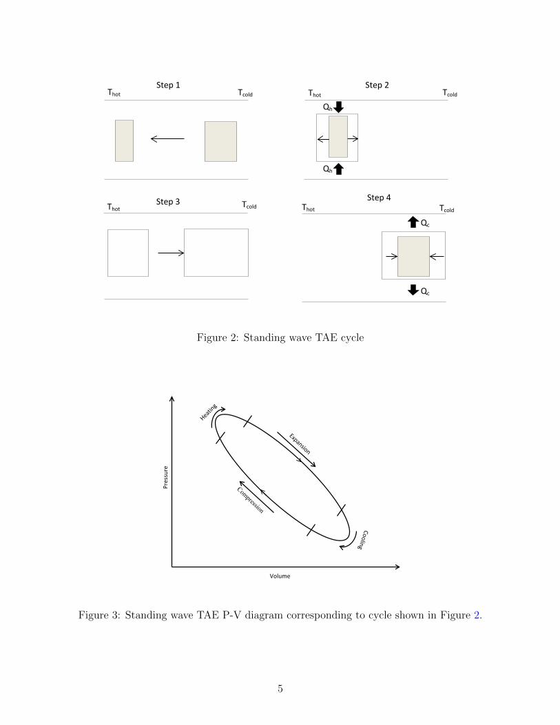
The standing wave cycle starts with the compression and movement of the gas towards
a hot heat exchanger. This part of the cycle is nearly adiabatic as the time it takes for the
gas to travel and the surface area of the pores facilitate very little movement of heat. In the
second step, the gas is heated by the stack walls, while simultaneously undergoing expansion.
It then moves toward the cold side heat exchanger, expanding along the way. This step of the
process, like the first, is adiabatic. The gas arrives at the cold heat exchanger at an elevated
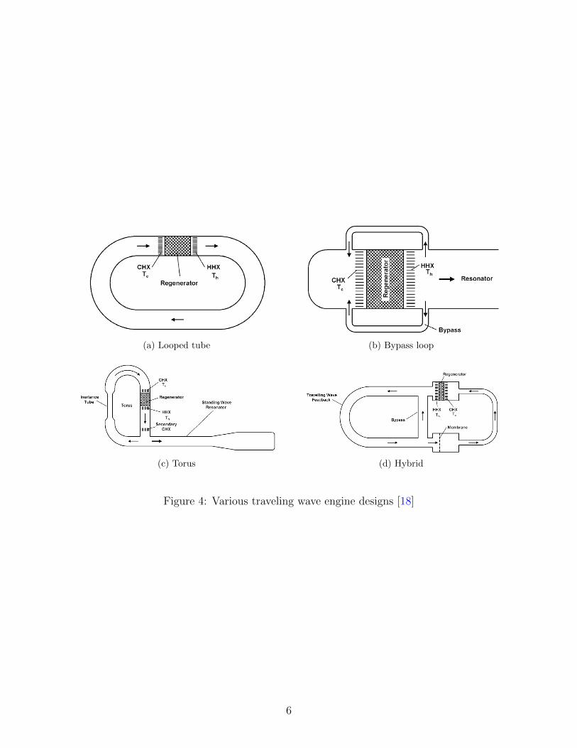
temperature, and is thus cooled, while contracting, completing the cycle [12]. Figure 2
demonstrates the steps of the cycle while Figure 3 shows the steps on a pressure-volume
diagram.
The cycle described above operates on the requirement of adiabatic movement in the first
and third steps. This is due to the out of phase pressure and velocity behavior of the standing
3

wave engine. It is necessary that the thermal expansion occurs at the highest pressure to
generate more work than is required to compress the gas for the extraction of heat at the
cold reservoir. Thus, if continuous heating and cooling occur, the net work pdV = 0. This
condition is achieved via the use of channels that are larger than the thermal penetration
depth of the gas. Thermal penetration depth, δk, is defined as the distance that heat can
travel through a gas at a certain frequency, as illustrated in Equation 1.1, where k is the
thermal conductivity, ρ is the density, cp is the coefficient of heat capacity, and ω is the
angular frequency of the sound wave. The thermal penetration depth is typically compared
to the hydraulic diameter, rh, of the channels used in the stack, calculated using Equation
1.2, where A is the area, and Π is the perimeter of the channel [13].
δk =
√2k
ρcpω(1.1)
rh =A
Π(1.2)
Standing wave engines, while simple, suffer a drawback in efficiency due to the irre-
versibility of the heat transfer process. The non-isothermal heating and cooling that are
isolated by the adiabatic movement impair the efficiency of the standing wave engine to
around 20% [14]. Theoretically, due to this irreversibility, standing wave engines also cannot
achieve the Carnot effeciency, while, as discussed below, traveling wave engines can.
1.2.2 Traveling Wave Engines
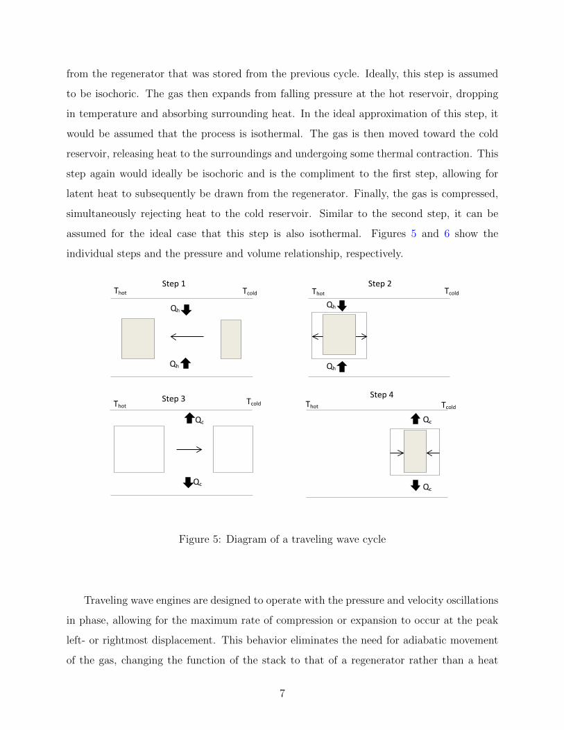
Traveling wave engines are, in general, slightly more complicated in design. Several designs
have been proposed and tested, with the more common ones shown in Figure 4. It can be
seen that each design employs a looped compliance, proposed and tested by first Ceperley
[8], then Backhaus et al. [15] and Ueda et al. [16], or a feedback inertance, first employed
by deBlok [17].
As aforementioned, the traveling wave thermodynamic cycle follows the same steps as
the Stirling cycle. The cycle begins with gas under high pressure moving toward the hot
reservoir, absorbing heat and slightly expanding along the way. Here, the gas abosrbs heat
4
Thot
Qc
Qc
Qh
Thot
Qh
Tcold
Tcold
Tcold
Tcold
Thot Thot
Step 1 Step 2
Step 3 Step 4
Figure 2: Standing wave TAE cycle
Pres
sure
Volume
Figure 3: Standing wave TAE P-V diagram corresponding to cycle shown in Figure 2.
5
(a) Looped tube (b) Bypass loop
(c) Torus (d) Hybrid
Figure 4: Various traveling wave engine designs [18]
6
from the regenerator that was stored from the previous cycle. Ideally, this step is assumed
to be isochoric. The gas then expands from falling pressure at the hot reservoir, dropping
in temperature and absorbing surrounding heat. In the ideal approximation of this step, it
would be assumed that the process is isothermal. The gas is then moved toward the cold
reservoir, releasing heat to the surroundings and undergoing some thermal contraction. This
step again would ideally be isochoric and is the compliment to the first step, allowing for
latent heat to subsequently be drawn from the regenerator. Finally, the gas is compressed,
simultaneously rejecting heat to the cold reservoir. Similar to the second step, it can be
assumed for the ideal case that this step is also isothermal. Figures 5 and 6 show the
individual steps and the pressure and volume relationship, respectively.
Qc
Qc
Qh
Qh
Qc
Qc
Qh
Thot
Qh
Tcold
Tcold
Tcold
Tcold
Thot Thot
Thot Step 1 Step 2
Step 3 Step 4
Figure 5: Diagram of a traveling wave cycle
Traveling wave engines are designed to operate with the pressure and velocity oscillations
in phase, allowing for the maximum rate of compression or expansion to occur at the peak
left- or rightmost displacement. This behavior eliminates the need for adiabatic movement
of the gas, changing the function of the stack to that of a regenerator rather than a heat
7

Figure 6: Traveling wave TAE P-V diagram corresponding to cycle in Figure 5 [18].
storage surface. The design of a traveling wave engine then requires for the channels to be
significantly smaller than that of a standing wave engine, particularly small enough to where
δk >> rh. This allows for nearly isothermal heat transfer through the cycle, allowing for the
traveling wave engine to theoretically be capable of reaching the Carnot efficiency.
1.3 MOTIVATION FOR THERMOACOUSTIC REFRIGERATION
The widest application of thermoacoustics can be seen today in its use in refrigeration and
cryogenic cooling. Most cooling demands are currently met via the use of vapor compression
and absorption cooling. However, TARs have several advantages over these systems, as
discussed below, that can help them increase their share in the market in an environmentally
sustainable way.
1.3.1 Absorption Cycles
Absorption cycles employ the use of a chemical solution to drive mixture and separation
of typically two compounds, such as water and lithium bromide. The use of two solutions
8

allows for evaporated water at low pressure to be absorbed into the solution, pressurized
using a low amount of energy, and again evaporated, recycling the lithium bromide solution.
The highly pressurized water can be again condensed at a higher temperature and after a
decrease in pressure, evaporated at a lower temperature to begin the cycle again. Figure 7
shows a simple diagram of an absorption cycle.
Generator
Expansion Valve
Evaporator
Condenser
Figure 7: Diagram of a typical absorption cycle
The major inputs of energy for absorption cycles are electric or shaft power into the pump
to bring the solution to a high pressure and heat at high pressure to evaporate the liquid.
Here, the absorption cycle has an advantage in the use of heat rather than mechanical energy,
as compared to the vapor compression cycle discussed below. Thus, a lower exergy source of
energy can be used to drive this cycle, such as waste heat from an industrial process, heat
given off by a combustion engine, or solar energy. Absorption cycles, however, suffer from
several drawbacks. They are much more complex than either vapor compression systems or
TARs and have a relatively low COP, typically around 0.68 for partially solar powered cycles
[19]. Additionally, when liquids such as ammonia are used in absorption cycles, extra care
must taken if the solution leaks since ammonia is an environmentally dangerous chemical.
9

1.3.2 Vapor Compression
Expansion Valve
Compressor
Evaporator
Condenser
Figure 8: Diagram of a typical VC cycle
Vapor compression (VC) is currently the dominant form of refrigeration, found in a range
of applications, from household air conditioners to industrial ice makers and gas liquifica-
tion. The VC cycle is very simple in its design, employing four basic stages: evaporation,
compression, condensation, and expansion, shown in the diagram in Figure 8. Similar to ab-
soption cycles, the evaporation stage is used to achieve cooling and the condenser to release
high pressure heat to the ambient air. However, in a VC cycle, the compressor replaces the
absorption system, simplifying the process. VC technology, however, has several drawbacks
in that it is limited to approximately 230K in a single stage and requires high exergy energy
(i.e. mechanical or electrical) to operate. This causes a major increase in complexity when
temperatures like that of liquid nitrogen and helium are desired. TARs, on the other hand,
have been reported to be able to achieve much lower temperatures, with Jin et al. reporting
120K [20] and Vanapelli et al. reaching a temperature as low as 50K [21].
10

1.3.3 Thermoacoustic Cooling
Thermoacoustic refrigerators can be assembled in several configurations, using either me-
chanical, or thermal energy to drive the thermoacoustic effect. TARs have several advan-
tages over the cycles discussed above. Both VC and absorption cycles require the use of
potentially dangerous refrigerants and are fairly complex systems, increasing the potential
for leaks. TARs benefit from use of inert gases like Helium and Argon, or can even be op-
erated with air, making them simple and safe. They also present a secondary advantage in
the use of cryogenic cooling. It is well-known that standard vapor compression refrigerators
(VCRs) have a limited lifespan due to the low temperatures the seals experience around the
moving parts. TARs bypass this need due to the lack of moving parts in the design. Thus,
when space is not limited, such as in cryocooling stations, or on large refrigeration trucks,
TARs have the potential to replace the current technology quite readily.
One of the main reasons why TARs have not been implemented on a large scale is based on
their inherently low coefficient of performance (COP), which is the ratio of cooling capacity
to input energy. Note that the COP is not an efficiency in the classical sense, and is thus not
bounded by 1. A benchmark of current cooling technology illustrates a spread of COPs of
traditional refrigeration between 2 and 6, varying with different working fluids, compressor
efficiencies, and operating temperatures [22]. On the other hand, TARs are still operating at
COPs of 1 to 1.2 [23, 24]. Limitations for the COP in TARs come from streaming, acoustic,
viscous, and thermal losses [23], which are discussed further in Ch. 2.
Fortunately, though, recent work has found that TARs and thermoacoustic engines
(TAEs) can be powered by waste heat, at input temperature levels that are not suitable
for powering VCRs [25]. This means that the practical level of the input energy is greatly
reduced, thus making waste heat-driven TARs/TAEs competitive with VCRs, since VCRs
require mechanical energy (often produced from electrical energy) to power the compressor.
However, beyond this COP comparison, another limiting factor for wide spread implemen-
tation of thermoacoustics is the physical size of TARs. If the resonator could be coiled as
opposed to being designed as a straight tube, the footprint of TAEs and TARs could be
reduced, and thus be advanced towards broader implementation. While theoretical models
11

for curvature behavior in relation to the thermoacoustic effect have previously been pro-
posed [26], there is currently a lack of computational models that accurately predict the
phenomenon.
1.4 GOALS OF THIS WORK
In this work, two thermoacoustic devices are designed and evaluated for their performance
in relation to pressure and temperature. A standing wave thermoacoustic device is designed
to establish temperature behavior patterns for the hot and ambient sides and compare the
temperature difference across the stack to the magnitude of pressure oscillations in the engine.
A traveling wave engine is then designed and evaluated for temperature behavior through
the regenerator to establish the intensity of the thermoacoustic effect via the temperature
difference.
12

2.0 THERMOACOUSTIC THEORY
2.1 LINEAR ACOUSTIC THEORY
First developed by Nikolaus Rott [27], linear acoustic theory is the first complete theory
that fairly accurately predicts behavior of thermoacoustic engines and refrigerators. While
Kramers [6] developed his theory before Rott, his derivation was based on the assumptions
of linearization of all equations and the boundary layer approximation. These were not able
to provide accurate predictions, leading Rott to further specify the problem by defining the
following assumptions:
(1) The gradient of the acoustic pressure in the radial direction is assumed to be zero,
(2) The average temperature and viscosity in the radial direction are negligible, and
(3) Axial heat conduction in the medium is negligible in comparison to the thermoacoustic
effect, and friction in the axial direction is neglected.
These assumptions are implied from the overall general assumption that the tube radius
is significantly smaller than the tube length, a crucial assumption that allowed for Rott to
achieve much more accurate predictions for the behavior of thermoacoustic devices. Be-
ginning with the continuity, momentum, and energy equations and assuming that u and
v undergo time variation given by the factor exp(iωt), the equations become, respectively:
13
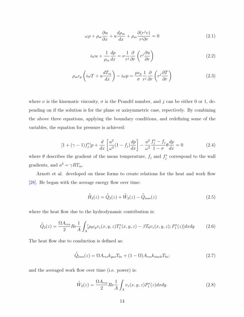
ωρ+ ρm∂u
∂x+ u
dρmdx
+ ρm∂(rjv)
rj∂r= 0 (2.1)
iωu+1
ρm
dp
dx= ν
1
rj∂
∂r
(rj∂u
∂r
)(2.2)
ρmcp
(iωT + u
dTmdx
)− iωp =
µcpσ
1
rj∂
∂r
(rj∂T
∂r
)(2.3)
where ν is the kinematic viscosity, σ is the Prandtl number, and j can be either 0 or 1, de-
pending on if the solution is for the plane or axisymmetric case, repectively. By combining
the above three equations, applying the boundary conditions, and redefining some of the
variables, the equation for pressure is achieved:
[1 + (γ − 1)f ∗j ]p+
d
dx
[a2
ω2(1− fj)
dp
dx
]− a2
ω2
f ∗j − fj1− σ
θdp
dx= 0 (2.4)
where θ describes the gradient of the mean temperature, fj and f ∗j correspond to the wall
gradients, and a2 = γRTm.
Arnott et al. developed on these forms to create relations for the heat and work flow
[28]. He began with the average energy flow over time:
¯H2(z) = ¯Q2(z) + ¯W2(z)− ¯Qloss(z) (2.5)
where the heat flow due to the hydrodynamic contribution is:
¯Q2(z) =ΩAres
2Re
1
A
∫A
[ρ0cpvz(x, y, z)T ∗1 (x, y, z)− βT0vz(x, y, z);P ∗
1 (z)]dxdy (2.6)
The heat flow due to conduction is defined as:
¯Qloss(z) = ΩAreskgasT0z + (1− Ω)AreskstackT0z; (2.7)
and the averaged work flow over time (i.e. power) is:
¯W2(z) =ΩAres
2Re
1
A
∫A
vz(x, y, z)P ∗1 (z)dxdy. (2.8)
14

Ares is defined as the cross-sectional area of the tube at a point z, A is the area of a single
pore, Ω is the porosity of the stack, kgas and kstack are the thermal conductivity values for
the the gas and stack, respectively, ∗ defines complex conjugation on the variable in question,
and Re indicates that the real part of the expression is being evaluated.
To develop the above relations to a functional form, the velocity in the z direction was
defined as:
vz(x, y, z) =F (x, y;λ)
iωρ0
dP1(z)
dz(2.9)
where λ = 21/2R/δv and F (x, y, ;λ) is a function that equals zero at the wall. The heat and
work flow then took the following form:
¯Q2(z) =ΩAres
2βT0
[Im
(P1z(z)P ∗
1 (z)
ρ0ω
F ∗(λT )− F (λ)
1 +Npr
)−
T0zβT0
cpρ0ω3
|P1z(z)|2 Im[F ∗(λT ) +NprF (λ)]
1−N2pr
] (2.10)
¯W2(z) =ΩAres
2Im
(P1z(z)P ∗
1 (z)
ρ0ωF (λ)
)(2.11)
Tijani et al. continued the development of the theory to provide heat and work flow
equations that are based on dimensionless parameters describing thermoacoustic devices
[29]:
Qcn = −δknD2sin2xn
8γ(1 + σ)Λ
(∆Tmntan(xn)
(γ − 1)BLsn
1 +√σ + σ
1 +√σ− (1 +
√σ −√σδkn)
)(2.12)
Wn =δknLsnD
2
4γ
[(γ − 1)Bcos2xn
(∆Tmntan(xn)
BLsn(γ − 1)(1 +√σ)Λ− 1
)−√σsin2(xn)
BΛ
](2.13)
In the above equations, xn is the center position of the stack, Lsn is the length of the stack,
A is the cross-sectional area, σ is the Prandtl number, δkn = δk/y0 is the normalized thermal
penetration depth, D is the drive ratio, γ is the ratio of isobaric to isochoric specific heats,
and B is the porosity of the stack. Additionally, Λ = 1 −√σδkn + 1
2σδ2kn. Tijani et al.
used these equations to provide a framework for designing thermoacoustic refrigerators with
optimized parameters for the highest COP, acoustic power, or cooling rate [30].
15
While the general theory of thermoacoustics is well understood, there is still much re-
search being conducted in the study of the losses that occur in TAEs and TARs. Application
of Tijani’s derivations presents possible COP values as high 1.8 for optimized design spec-
ifications. However, due to various losses, these values are, in fact, much lower than is
theoretically predicted. Acoustic, streaming, and viscous losses have been extensively re-
searched in the past and have been shown to be major contributors to the energetic losses in
thermoacoustic devices. These losses will be explained as part of the influencing factors in
the behavior of the standing wave device examined in this work. Thermal losses are less un-
derstood, as it is harder to quantify their effects due to the parallel nature of their behavior
with the thermoacoustic effect. Zink et al. [31, 32] proposed methods for quantifying these
losses, showing significant effects due to convection and radiation.
2.2 STREAMING LOSSES
Streaming losses can be identfied as the energy losses that are caused by the movement of
the gas in the thermoacoustic device. While gas displacement in the stack or regenerator
of the thermoacoustic device is crucial to that device’s performance, other gas movements
have been identified and observed in various devices that are detrimental to the performance.
Gedeon and Rayleigh streaming mechanisms have been found to contribute signficantly to
the overall losses found in thermoacoustic engines and refrigerators, and have been noted to
have the largest effect on refrigerators and traveling wave engines.
2.2.1 Gedeon Streaming
Gedeon streaming is defined as the acoustic streaming around a torus. This streaming occurs
in traveling wave looped tube engines and pulse tube design refrigerators. The mechanism
of this streaming occurs as gas particles travel in the regenerator through a complete cycle.
While it would be expected for each particle to assume the original position at the end of
each cycle, it is found that the distance that a particle covers from the hot to the cold side
16
is not the same as in the opposite direction. Thus, a net mass flow, as shown in Figure 9, is
experienced and is exacerbated by the fact that there is no hindering mechanism in a torus
or pulse tube design to prevent circulation of the particles. This results in a heat transport
mechanism that is parallel to the thermoacoustic mechanism, causing a heat load on the
cold side and thus decreasing efficiency.
Gedeon streaming has been evaluated by several groups, both experimentally and analyt-
ically. Olson et al. [33] have shown the effect of this mechanism in pulse tube refrigerators,
demonstrating that it’s suppression can increase performance. They established that the
oscillations approximately a penetration depth away from the pulse tube wall cause a drift,
establishing a parabolic mass flux profile, as shown in Figure 10, and causing convection of
heat. Using linear acoustic theory, presented above, they were able to establish an expression
for the streaming mass flux,
m2,w =|p1||u1|a2
[(3
4+
(γ − 1)(1− bσ2)
2σ(1 + σ)
)cosθ +
(3
4+
(γ − 1)(1− b)√σ
2(1 + σ)
)sinθ
]+
ρm|u1|2
ω
[3
4
dA/dx
A+
(1− b)(1−√σ)
4(1 + σ)(1 +√σ)
dTm/dx
Tm
](2.14)
An analytical approach was conducted by Gusev et al. [34], using the measure of en-
thalpy flux to demonstrate that the mechanism has a significant impact. Other groups, such
as Penelet et al. [35] have shown that streaming has a positive effect on thermoacoustic
performance, providing amplification of the thermoacoustic effect. Overall, however, there
have been numerous efforts to suppress Gedeon streaming.
One method that has been shown to increase performance in engines was proposed by
Swift et al. [36] . Their group demonstrated an increase in performance through the use
of a flexible membrane inside the torus. This membrane, of course, introduces an acoustic
impedance, causing an increase in acoustic losses in the engine. Olson et al. [33] proposed a
different method for suppressing streaming using a tapered pulse tube, producing significant
results.
17

Figure 9: Illustration of
net mass flow occurence in
pulse tube [33].
Figure 10: Mass flux profile
in pulse tubes from central
axis to wall [33].
2.2.2 Rayleigh Streaming
While Gedeon streaming is specific to traveling wave designs, Rayleigh streaming is an
occurence that can be found in both standing and traveling wave engines, and has been
shown to be equally significant in refrigerators. This method of streaming stems from the
interaction of the oscillating flow and the the various surfaces inside the engine or refrigerator.
First proposed by Rayleigh in 1896, this method was investigated by several groups, and was
experimentally proven by Gaitan et al. [37]. Yazaki et al. [38] investigated this streaming
mechanism further using Doppler velocimetry to examine thermoacoustic work flow. They
were able to obtain results that agreed with theory and images, such as Figure 11, to show
that the streaming is, in fact, significant.
Thompson et al. [39] used Laser Doppler Anemometry (LDA) and burst spectrum anal-
ysis (BSA) to obtain velocity field measurements, such as the one in Figure 12, showing
streaming inside a standing wave device. Using these measurements, they were able to show
the relationship between the axial acoustic velocity and the axial streaming velocity shown
in Figure 13.
18

Figure 11: Image of streaming taken us-
ing Doppler velocimetry [38].
Figure 12: Velocity filed observed using
LDA and BSA [39].
Figure 13: Relation between axial acoustic and axial streaming velocities [39].
19

2.3 ACOUSTIC LOSSES
There are several mechanisms of acoustic losses that take place in thermoacoustic devices.
Resonator shape, uneven joints, and open end conditions can have a significant impact on
acoustic wave propagation. A signficant amount of research has been conducted on improving
the acoustic efficiency of engines. Several groups have identfied the use of tapered resonator
tubes to help increase performance.
As discussed above, there are several loss mechanisms that cause a decrease in perfor-
mance, and solutions to decrease the effects of some losses will cause other losses to increase.
This is particularly true in refrigeration, where it is beneficial to separate driving and refrig-
eration stacks to decrease/eliminate convective losses. In both traveling and standing wave
refrigerators, this increases the complexity of the design and can create a large increase in
impedance caused by the resonance body.
Figure 14: Real and imaginary parts of F (λ) for various pore geometries [28].
Stack design has also been examined. Arnott et al. [28] analytically examined work and
heat flows for various pore geometries using equations 2.10 and 2.11. They determined that
the primary influence on the work and heat flow is the function F (λ). Thus, they evaluated
20

this function for both its real and imaginary parts for various values of λ. As shown in Figure
14, parallel plate stacks have the largest imaginary part at a value λc ≈ 3.2, demonstrating
that they will produce the strongest thermoacoustic effect.
2.4 VISCOUS LOSSES
It is well-known that movement of a fluid will experience viscous energy dissipation and,
in some cases, a significant amount of viscous heating. This form of energy dissipation
is clearly present in stacks/regenerators, as the large surface area to volume ratio causes
the presence of significant dissipation through both methods. Atchley et al. [40–42] have
shown that these two forms of energy dissipation are, in fact, the dominant mechanisms in
thermoacoustic devices. They presented the following form for calculating the losses in the
heat exchangers
dWhx =1
2ShxRe
P 2Aω
ρma2i
[(1 +
(γ − 1)
1 + εsfk
)cos2φ(x)− (1 + l/y0)
2
1− fvsin2φ(x)
]dx (2.15)
Figure 15: Experimental results compared to analytical forms for heat compared to the
tempertaure difference [40].
21

where Shx is the cross-sectional area of the heat exchanger, PA is the peak pressure amplitude,
a is the speed of sound, fk and fv are function of the thermal and viscous penetration depths,
and y0 is the plate half-spacing. The analytical forms were examined against experimental
results for a thermoacoustic prime mover below onset of self-oscillation, shown in Figure 15,
providing close agreement between the data and the predictions. In the next section, thermal
losses are examined more closely and compared to the viscous losses that were discussed here.
2.5 THERMAL LOSSES
Thermal losses in thermoacoustic devices are less understood than the other mechanisms
discussed above. Since, as discussed, thermoacoustic devices operate on the basis of temper-
ature gradients, there will be nontrivial losses due to conduction through the stack as well as
convection to the medium. Due to the parallel nature and interaction behavior of the mech-
anisms, however, it is more difficult to quantify the impact of these losses experimentally.
Losses via conduction have been mentioned in several studies. Organ et al. [43] referred
to these losses in their evaluation of mechanical Stirling engines. Referred to as “thermal
shorting,” their group discussed how heat flow paths are created in regenerators built from
stacked wire meshes. Chen et al. [44] investigated the COP of a thermoacoustic refrigerator
with regard to the temperature difference applied across the stack, arriving at a conclusion
that the thermal conductivity of the stack noticeably influences the performance. Holmberg
et al. [45] used software to determine the significance of several viscous and thermal losses
in stacks and on a system level. Their group evaluated a thermally driven thermoacoustic
refrigerator consisting of two stacks and three heat exchangers, assembled in a series config-
uration to achieve cooling at the surface facing the open end of the resonator, as shown in
Figure 16. A system level analysis, seen in Figure 17, shows that the cooling work is only a
small portion of the overall thermal input. Due to the design used in the analysis, the largest
portion was found to be in the viscous losses of the high temperature heat exchanger with
the viscous thermoacoustic losses becoming a close second at high heat input. An analysis
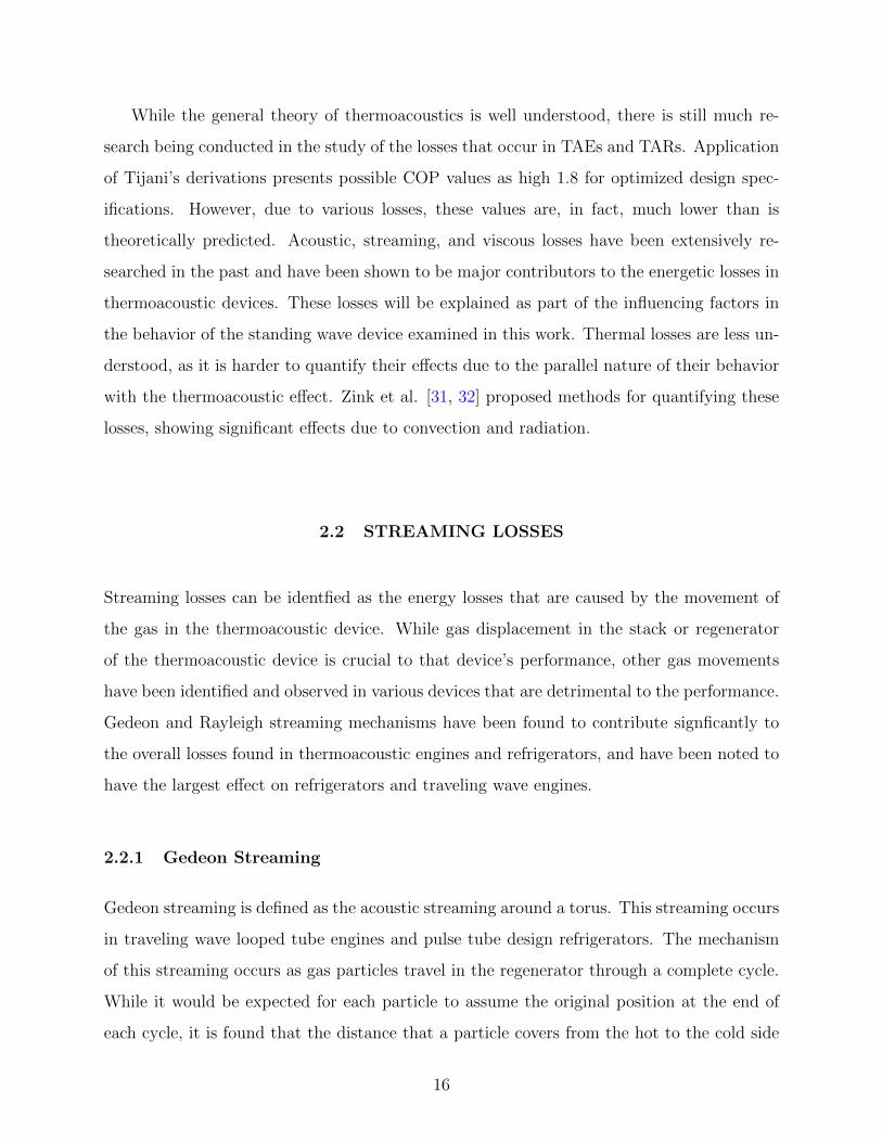
of the heat exchanger control volume, shown in Figure 18, showed a signficant amount of
22

thermal loss due to the conduction in the stack, indicated as Qcond,1avg, despite the stack
being designed using ceramic material.
Figure 16: TAR design [45]
Figure 17: Thermoacoustic refrigerator ther-
mal and viscous losses [45].
Holmberg’s group presented an estimate for the magnitude of losses in the thermoacoustic
refrigerator, including conduction loss through the ceramic stack. A thorough investigation
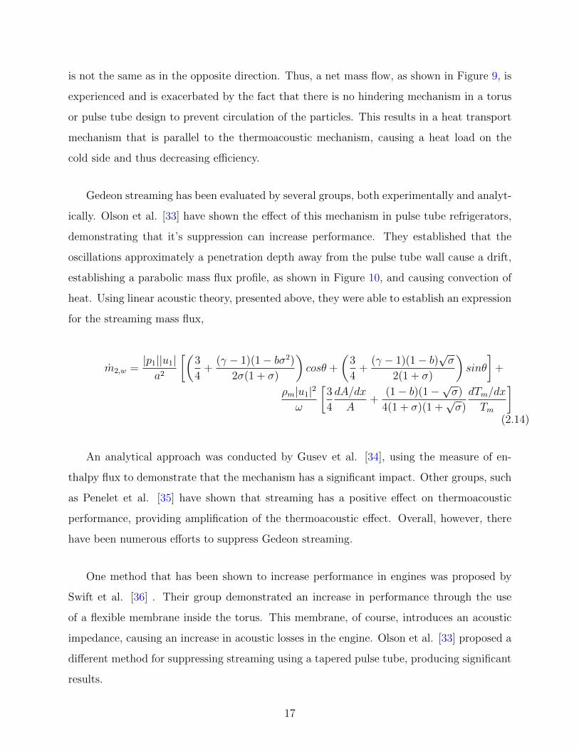
in how this loss varies with stack materials was presented by Zink [32, 46] in his investi-
gation of conductive, convective, and radiative losses for aluminum, stainless steel, copper,
ceramic, and brass stacks. Using a quarter-wavelength thermoacoustic engine, he evaluated
the acoustic performance with respect to input power, as seen in Figure 19. Ceramic stacks
were found to perform significantly better than other materials. However, an evaluation of
convective and radiative losses, seen in Figures 20 and 21, presented a drawback of the lower
conduction material in the increase of the temperature at the hot side and increase in both
convection and radiation.
23
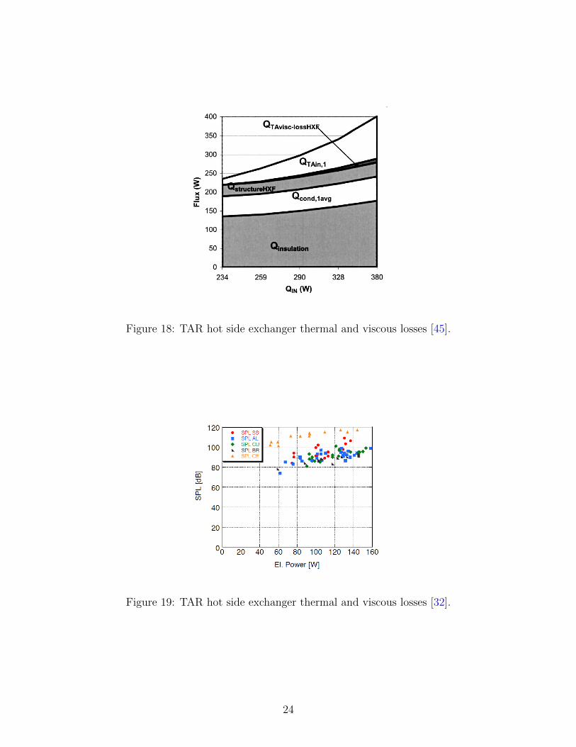
Figure 18: TAR hot side exchanger thermal and viscous losses [45].
Figure 19: TAR hot side exchanger thermal and viscous losses [32].
24

Figure 20: Convective losses [32] Figure 21: Radiation losses [32]
25

3.0 STANDING WAVE INVESTIGATION
As discussed in the previous chapter, although recent research has increasingly focused on
thermal behavior of thermoacoustic devices, much more work needs to be done. Additionally,
as mentioned in Chapter 1, for thermoacoustic devices to be competitive in the marketplace,
their efficiency must be improved while increasing the flexibility of their operating footprint.
To that end, the goal of this work is to perform experimental investigations to determine:
(a) how curvature affects the total temperatures on the hot and cold side, and
(b) how curvature affects the oscillation behavior (i.e. does sound pressure level decrease as
curvature increases).
3.1 DESIGN AND CONSTRUCTION
3.1.1 Stack Length and Position
As mentioned above, the quarter-wavelength resonator design operates with a pressure node
at the open end of the resonator and an antinode at closed end. Simultaneously, the velocity
operates 90 out of phase with the pressure, resulting in a node at the closed end of the
resonator. As discussed above, both pressure and velocity oscillations are required for the
standing wave cycle to operate. Thus, stack positioning at either end of the resonator
does not facilitate effective acoustic generation. Studies on thermoacoustic refrigeration
optimization [25, 30] show that it is most efficient for the stack position to be close to
the pressure antinode. Tijani et al. [30] have also shown that as stack size increases, the
optimal center position of the stack moves further from the pressure antinode. Their group
26

has also shown that the COP increases and the acoustic power decreases as stack length
decreases. Both groups derived optimization methods, Tijani’s group’s method based on
cooling and acoustic power and Babei and Siddiqui’s method [25] on cooling power and cold
side temperature. Babei and Siddiqui’s group has also shown that many similarities can
be drawn between TARs and TAEs, allowing for the above mentioned relationships to be
applied for TAEs.
These guidelines were implemented in the design of the stack and positioning, for creation
of a standing wave device for experimental testing. Due to the brittle nature of the ceramic,
a stack length of 2 inches was chosen, corresponding to a normalized length of 0.05. Due to
the thermal sensitivity of the microphone, the center positioning of the stack was chosen to
be approximately 5 inches, corresponding to a normalized distance of 0.125. For the goal of
this study, an optimal stack length and position were not identified, as the curvature of the
resonator would affect these parameters in ways not well understood.
3.1.2 Pore Geometry and Size
The stack was chosen from a readily available ceramic monolith with square channels. Several
sizes were available, and thus it was important to choose a stack that would meet the
requirements of a standing wave engine. To achieve the adiabatic requirement, there must
be poor thermal contact between the stack and the working fluid. Using air as the working
fluid, and the nominal frequency of 80Hz, it was determined that the thermal penetration
depth was 0.332mm. A stack with square channels of 1.45mm was chosen as an initial size.
The ratio of the hydraulic radius to the thermal penetration depth was found to be 1.09,
which agreed with the requirement for the operation of standing wave engines, allowing the
use of the stack in the engine design.
3.1.3 Resonator
The resonator was chosen for the engine to operate as a quarter-wavelength engine. For a
80Hz wavelength, this corresponded to a length of the 1000mm. The assembly was con-
structed using a stainless steel stack housing and flexible PVC tubing of 3.9mm thickness
27

(the inner diameter of both was 52.5 mm). The two components were joined by a flange with
the stainless steel portion closed at the end and the flexible tubing left open. The flexible
PVC tubing was used to acquire the proper curvatures (0, 15, 30, and 45), precalculated
using simple geometry and mounted horizontally. To prevent deformation of the flexible tub-
ing while bending, the maximum curvature was limited to 45. The assembly was mounted
such that the open end would face an unimpeded volume of air at atmospheric conditions
of at least 1 meter in radius from the open end. The curved section was constructed to be
approximately 500mm in length, following the model shown in Figure 22.
Curvature: 0o 15o 30o 45o Microphone Stack
Hot side T-couples and heating coil
Ambient side T-couples
Flexible tubing
Figure 22: Diagram of standing wave device used in testing
3.1.4 Data Acquisition
The stack was heated with 22-WG nickel-chrome wire and an DC power source. It was
mounted in the pattern of a heating coil, shown in Figure 23. Its resistance was RH = 2.25Ω
(measured at room temperature). During testing a constant voltage input of 15V was passed
through the wire. To record temperatures, four K-type thermocouples were inserted and
cemented into each end of the stack. Hot side thermocouples were mounted equidistant
from the sides of the coil and approximately 1.5mm into the stack. Figure 23 shows the
position for the hot side thermocouple mounting. The ambient side thermocouples were
mounted in a pattern similar to the hot side. Sound output was recorded with a PCB
130D20 array microphone that was mounted in the center of the closed end of the tube.
The data acquisition was performed in LabView. The sound pressure level was recorded
28

simultaneously with the temperature to observe any correlation that they would show. The
output of each curvature was recorded in three separate 300 second (5 minute) spans with a
sample rate of 0.1 seconds. Each curvature was tested three times to increase the confidence
in the temperature and sound pressure level readings. Each test was executed by starting
the engine from ambient conditions, allowing it to approach steady behavior, and running
the testing interval. A 5V initial run was examined for the transient response from ambient
temperature, shown in Figure 24. An exponential fit was applied to the data and a time
constant of τ5V = 85.4 seconds was identified for the transient response. The 5V test showed
a temperature increase of 102C, approximately 1/3 in magnitude of the 15V results, shown
in the next section. As the magnitude of temperature increase matched the magnitude of
voltage input, similar behavior was assumed, implying a time constant of approximately 3
times greater than the 5V test run time constant. With this information, a startup time
of 20 minutes was used for the 15V tests, corresponding to 4.7 time constants (τ15V ≈ 255
seconds). It was later observed that slower time constants appeared to additionally affect
the engine, causing small transient changes in each run. These are assumed to be due to the
heating of the housing.
Electrodes
Heating Coil
Thermocouple Positions
Stack
Figure 23: Diagram of hot side of stack assembly
29
0 100 200 300 4000
50
100
150
Time (sec)T
empe
ratu
re (o C
)
Recorded TemperaturePredicted behavior
Figure 24: Initial response of SWTAE to 5V input
3.2 RESULTS: TEMPERATURE BEHAVIOR
In order to show the effect of resonator curvature on the thermoacoustic effect, we averaged
the recorded readings of the four hot and ambient thermocouples, first for the individual runs,
as seen in Figure 25 with the hot side temperature on the top, the ambient side temperature in
the middle, and the SPL on the bottom, then the three runs together, displayed in Figures 27
and 29, acquiring an overall average for each curvature. A frequency of occurence study was
conducted for each side, seen in Figures 26 and 28. Finally, a single value average hot
and ambient side temperature was calculated at 95% confidence and a regression analysis
was performed to quantify a relationship between temperature and curvature, as seen in
Figures 30 and 31. The temperature trends seen in these figures are discussed below.
3.2.1 Hot Side Behavior
The range of the individual hot side run averages spans approximately 18C. The individ-
ual runs also show a general trend of increase in temperature with curvature. While this
general trend is visible, there is obvious overlap in the averages of the individual runs, par-
ticularly between the 0 curvature and 15 curvature. Due to this diffuculty, the individual
run temperature values were evaluated in a histogram to observe the temperature occurence
30

behavior, as seen in Figure 26. The histogram shows that individual runs clearly show peaks
in frequency with each curvature, with the 45 and the 15 curvatures showing single peak
behavior, and the 0 and 30 curvature showing two peak behavior. To better define the
relationship between curvature and hot side temperature, the individual runs were averaged
and displayed in Figure 27. The relationship of temperature with time appears relatively
horizontal, implying that the hot side achieves steady state. The spacing between the av-
erages stays fairly equal, and thus, a linear relationship can be predicted. The results of a
linear regression analysis are discussed below.
0 100 200 300
325
330
335
340
345
350
355
360
Time (sec)Te
mpe
ratu
re (o C
)
Run1Run 2Run 3
0 100 200 300
325
330
335
340
345
350
355
360
Time (sec)
Tem
pera
ture
(o C)
0 100 200 300
325
330
335
340
345
350
355
360
Time (sec)
Tem
pera
ture
(o C)
0 100 200 300
325
330
335
340
345
350
355
360
Time (sec)
Tem
pera
ture
(o C)
0 100 200 30060
65
70
75
80
Time (sec)
0 100 200 30060
65
70
75
80
Time (sec)
0 100 200 30060
65
70
75
80
Time (sec)
0 100 200 30060
65
70
75
80
Time (sec)
0 100 200 300156
157
158
Time (sec)
Sou
nd (d
B)
0 100 200 300156
157
158
Time (sec)
Sou
nd (d
B)
0 100 200 300156
157
158
Time (sec)
Sou
nd (d
B)
0o Curvature 15o Curvature 30o Curvature 45o Curvature
0 100 200 300156
157
158
Time (sec)
SP
L (d
B)
Figure 25: Hot and ambient side temperature and SPL results for each of 3 runs for all
curvatures
31

340 345 350 355 360 3650
100
200
300
400
500
600
Temp
Occ
uren
ce
0o 15o 30o 45o
Figure 26: Hot side average histogram for each curvature.
0 50 100 150 200 250 300345
350
355
360
Time (sec)
Tem
pera
ture
(C
o )
0o 15o 30o 45o
Figure 27: Hot side averages for each curvature
32

3.2.2 Ambient Side Behavior
The ambient side individual runs fail to show any meaningful pattern, spanning a range of
approximately 7C. A general increase in temperature with time appears for several of the
individual runs. A histogram analysis of the temperatures, shown in Figure 28, shows that
there is significant overlap and multiple peak behavior for each curvature. An analysis of the
average ambient side behavior in Figure 29 shows that the 0 curvature shows the largest
increase in temperature with respect to time. The other curvatures also show a pattern of
increase with time, but appear to be more horizontal. From this, it can be concluded that
the ambient side did not achieve full steady state behavior during the runs as was originally
expected. A possible reason for this could be the gradual heating of the stack and the steel
housing, due to the leaching of heat from the hot side. A weak trend can be predicted based
on the 15, 30, and 45 curvatures of decreasing temperature with respect to an increase in
curvature. As discussed below, this trend is further evaluated using a regression analysis.
64 66 68 70 72 74 760
100
200
300
400
500
600
700
Temp
Occ
uren
ce
0o 15o 30o 45o
Figure 28: Ambient side average histogram for each curvature.
33

0 50 100 150 200 250 30050
51
52
53
54
Time (sec)
Tem
pera
ture
(C
o )
0o 15o 30o 45o
Figure 29: Ambient side averages for each curvature
3.2.3 Trends Between Temperature and Curvature
To better quantify the relationship between average hot side temperature and curvature,
an analysis of the total averages for each curvature was performed and displayed with the
predicted error of each curvature at 95% confidence, as seen in Figures 30 and 31. The
analysis shows a very strong correlation between the curvature and the average hot side
temperature with an R-squared value for the relationship of 0.9959. The overall spread of
the error in the prediction stays at an acceptable level for each curvature and does not show
any major change between curvatures. A similar analysis was performed on the ambient
side average temperatures. However, unlike the hot side, the ambient side showed little
correlation between curvature and temperature. The average value for the 0 curvature
appears to be significantly lower than that of the other curvatures. An analysis of the values
for the remaining curvatures produces a relatively strong correlation, with an R-squared
value of 0.8129. However, this value does not account for the significantly large spread of
error in the values, thus reducing the validity of any relationship present in the ambient
data.
34

−5 0 5 10 15 20 25 30 35 40 45 50
340
345
350
355
360
365
370
Curvature (degrees)
Tem
pera
ture
(C
o )
Figure 30: Hot side overall averages with linear regression prediction.
−5 0 5 10 15 20 25 30 35 40 45 50
60
65
70
75
80
Curvature (degrees)
Tem
pera
ture
(C
o )
Figure 31: Ambient side overall averages.
35

3.3 RESULTS: ACOUSTIC BEHAVIOR
Above, we discussed the effect of resonator curvature on the temperature throughout the
stack. Next we must discuss the effect of curvature on the pressure behavior of each TAE
design as the sound output is the primary metric in the characterization of thermoacoustic
devices.
3.3.1 General Oscillation Behavior
As mentioned above, the Sound Pressure Level (SPL) was recorded simultaneously with the
temperature behavior. Figure 25 shows the individual recorded levels for each run. While an
overall decrease in the pressure level is present, there is significant overlap between the 0 and
the 15 curvatures. The overlap between other curvatures is minimal. The SPL data spanned
a range of ≈ 2dB, with a minimum of approximately 156.4dB, corresponding to pressure
amplitudes between 1300 and 1600Pa. Averaging the runs for each curvature produces
a better defined pattern of decreasing SPL with curvature. While the relative spacings
between the 15 and 30 curvatures and 30 and 45 curvatures appear approximately equal,
the spacing between the 0 and 15 curvatures is significantly smaller. This behavior presents
a difficulty in predicting a relationship between SPL and curvature, which is discussed below.
3.3.2 Trends Between SPL and Curvature
The SPL was averaged to a single point for each curvature with error at 95% confidence.
No immediate linear relationship was clear, and thus both linear and quadratic predictions
were tested. The linear prediction showed a very good correlation of 0.958. However, the
quadratic prediction shown in Figure 34, showed a nearly perfect correlation of 0.998, thus
implying a quadratic relationship between curvature and SPL, at least for this limited data
set. This data has been collected only on a limited span of curvatures and so this relationship
cannot be extrapolated to increased curvatures, such as 90 or more. Also, the amount of
error present in the data suggests that the relationship, however well defined, may prove
unreliable, due to the large amount of overlap of the error.
36

The sound and hot side temperature behavior both provided the expected relationships.
It was thus of importance to evaluate the interaction between temperature and acoustic
pressure. The difference in temperature between the hot and ambient sides was evaluated
against the acoustic pressure, as shown in Figure 35. A strong relationship can be seen
between the temperature difference and the acoustic pressure, showing a linear decrease of
acoustic pressure with increase in the temperature difference. This behavior is expected as
the temperature difference between the hot and ambient sides of the stack is inversely pro-
portional to the amount of energy transfer that is occuring. A large difference in temperature
implies low energy transfer and a lower presense of the thermoacoustic effect. Similarly, a
smaller temperature difference implies higher energy transfer. It can be concluded that the
relative intensity of the thermoacoustic effect, identified with pressure amplitude (and thus
acoustic power), can be measured using a temperature difference across the stack. These
findings are utilized in the investigation of the traveling wave engine described below.
156 156.5 157 157.5 158 158.50
50
100
150
200
250
300
350
400
450
500
SPL
Occ
uren
ce
0o 15o 30o 45o
Figure 32: Sound Pressure Histogram
37

0 50 100 150 200 250 300156.5
157
157.5
158
Time (sec)
SP
L (d
B)
0o 15o 30o 45o
Figure 33: Average SPL for each curvature.
−5 0 5 10 15 20 25 30 35 40 45 50156
156.5
157
157.5
158
158.5
Curvature (degrees)
SP
L (d
B)
Figure 34: Average SPL with regression analysis.
38

270 275 280 285 290 295 300156
156.5
157
157.5
158
158.5
Temperature Difference Across Stack Thot
−Tambient
(oC)
SP
L (d
B)
Figure 35: Sound Pressure vs. Temperature Difference
39

4.0 TRAVELING WAVE INVESTIGATION
The investigation of curvature on the thermoacoustic effect in standing wave engines pro-
vided insight into the relationship between the thermal behavior of the stack and the acoustic
behavior of the engine. We observed that curvature creates increased losses and quantified
the effect of the losses. A logical extension of these findings could then be to apply them to
traveling wave thermoacoustic devices. However, there is still a large gap in our understand-
ing of thermal effects in the more complicated geometry of traveling wave devices. Before
any sort of future study of the effect of curvature can occur, these thermal effects must first
be quantified.
Therefore, the goal of the next component of this study was to examine the thermal
behavior of the regenerator in a looped tube traveling wave thermoacoustic engine. The
established thermal patterns were then examined for various placements of the regenerator
inside the looped tube device to observe the effect of placement on the intensity of the
thermoacoustic effect.
4.1 DESIGN AND CONSTRUCTION
4.1.1 Resonator
A looped tube design was chosen for this investigation. Previous investigations have been
conducted on the looped tube design by Ceperley et al. [47] and Yazaki et al. [38], with
Yazaki’s group identifying large viscous losses, suggesting an increase in acoustic impedance.
Swift et al. [36] modified the design by adding a resonator to the loop, creating a torus
40

type engine. This, however, created a secondary system for losses that were later shown by
Hu et al. [48] to significantly decrease the efficiency, compared to what had previously been
reported. Backhaus et al. [49] have demonstrated that a looped tube engine can be used
in tandem with an electric generator, achieving a thermal to electric effeciency of 18%. It
can thus be observed that looped tube engines have the potential for efficient conversion of
input heat to electric work as well as refrigeration.
A total length of 92in was implemented as a design parameter, leading to an operating
frequency of 146Hz in the first mode, with air as the working fluid at atmospheric pressure.
The loop-tube was designed using 2 inch nominal diameter schedule 40 PVC and steel pipe,
with the heating element positioned in the steel portion of the device, to prevent melting
of the PVC. The heating element was designed to have the same nominal resistance as the
element in the standing wave design. The straight portions of the pipe were approxmately
34 inches long, with the turns approximately 12 inches in length. Standard 90 elbows were
joined to the PVC pipe using PVC cement to create the 180 turns required for the loop.
The PVC portion of the loop-tube was joined to the steel portion using 4-bolt flanges, with
air tightness assured using full-face gaskets. A picture of the device can be seen in Figure
36 with a close up on the steel portion containing the stack shown in Figure 37.
4.1.2 Regenerator
As was discussed above, standing wave and traveling wave engines operate under similar
cycles. Several key differences, however, allow traveling wave engines to inherently operate
more efficiently than standing wave engines. One such difference lies in the design of the
regenerator. Stacks in standing wave engines require the hydraulic diameter to be larger
than the thermal penetration depth. Regenerators in traveling wave engines, on the other
hand, require a smaller hydraulic diameter to facilitate reversible heat transfer between the
medium and the regenerator. Stacked wire meshes have previously been implemented as
a regenerator design [36]. However, as discussed above, Zink et al. [32] have found that
higher conductivity materials cause secondary losses by carrying heat via conduction. A
41

Figure 36: Picture of traveling wave TAE
Figure 37: Housing design used to insure
air tightness.
Figure 38: Regenerator used in the con-
struction of the TAE.
42
square channel ceramic porous material was thus implemented. A pore size of 1.092mm was
chosen, providing a ratio of 0.89 between the hydraulic diameter and the thermal penetration
depth.
The regenerator, seen in Figure 38, was made using a porous ceramic material (found in
catalytic converters in automobile mufflers) with a hole density of approximately 20 holes
per inch. The stack was machined to fit into the pipe, and cut to approximately 3.5 inches
in length. It was then modified to include an electric heating coil on one side. The heating
portion of the coil was designed using 22AWG wire with the lead wires built using 18AWG
wire to minimize heat dissipation through wire not directly in contact with the stack.
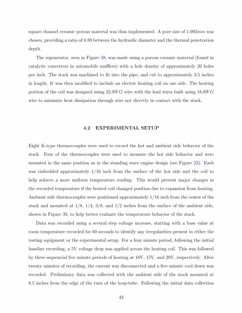
4.2 EXPERIMENTAL SETUP
Eight K-type thermocouples were used to record the hot and ambient side behavior of the
stack. Four of the thermocouples were used to measure the hot side behavior and were
mounted in the same position as in the standing wave engine design (see Figure 23). Each
was embedded approximately 1/16 inch from the surface of the hot side and the coil to
help achieve a more uniform temperature reading. This would prevent major changes in
the recorded temperature if the heated coil changed position due to expansion from heating.
Ambient side thermocouples were positioned approximately 1/16 inch from the center of the
stack and mounted at 1/8, 1/4, 3/8, and 1/2 inches from the surface of the ambient side,
shown in Figure 39, to help better evaluate the temperature behavior of the stack.
Data was recorded using a several step voltage increase, starting with a base value at
room temperature recorded for 60 seconds to identify any irregularities present in either the
testing equipment or the experimental setup. For a four minute period, following the initial
baseline recording, a 5V voltage drop was applied across the heating coil. This was followed
by three sequencial five minute periods of heating at 10V, 15V, and 20V, respectively. After
twenty minutes of recording, the current was disconnected and a five minute cool down was
recorded. Preliminary data was collected with the ambient side of the stack mounted at
8.5 inches from the edge of the turn of the loop-tube. Following the initial data collection
43
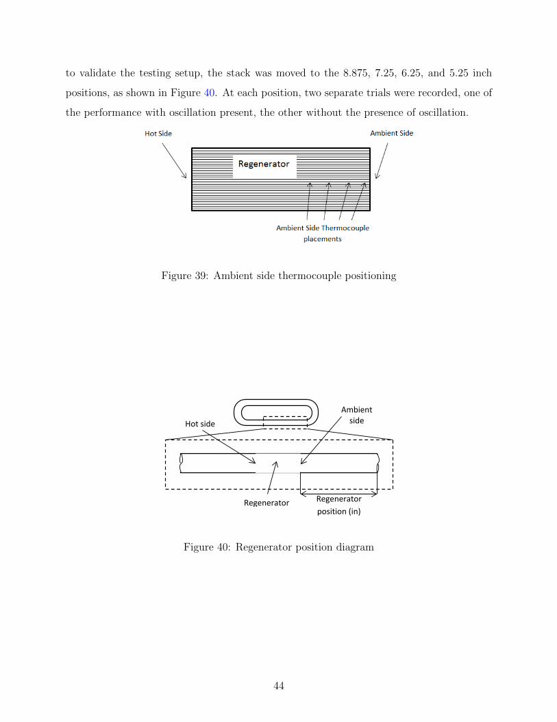
to validate the testing setup, the stack was moved to the 8.875, 7.25, 6.25, and 5.25 inch
positions, as shown in Figure 40. At each position, two separate trials were recorded, one of
the performance with oscillation present, the other without the presence of oscillation.
Figure 39: Ambient side thermocouple positioning
Regenerator position (in)
Regenerator
Hot side
Ambient side
Figure 40: Regenerator position diagram
44

4.3 RESULTS: STACK POSITIONING EFFECTS ON
THERMOACOUSTIC BEHAVIOR
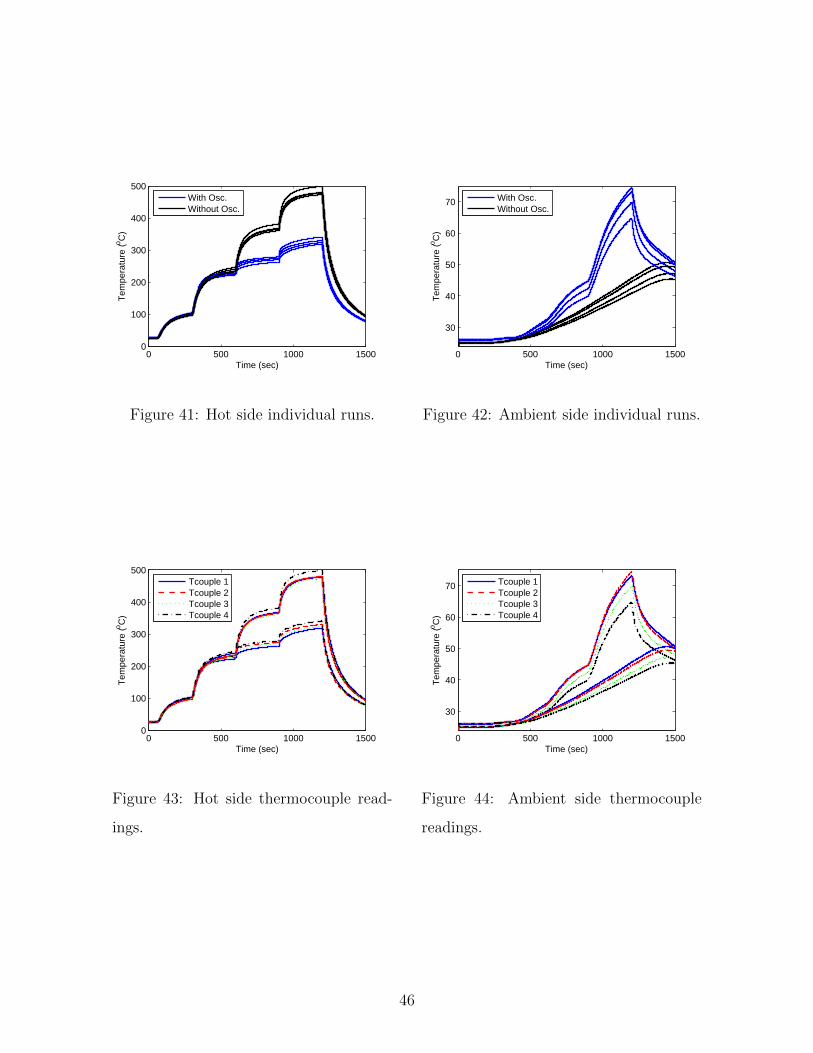
4.3.1 Patterns In Thermoacoustic Behavior
Preliminary data were collected to study the behavior of the individual thermocouples in
relation to the presence and the lack of oscillation. Figures 41 and 42 show the behavior
of the hot and ambient sides, respectively. The maximum temperature difference between
the oscillation and no oscillation runs on the hot side was approximately 154C, while the
maximum temperature difference for the ambient side was approximately 27C. Figures 43
and 44 show the same data, but are color coded to show the behavior of the individual
thermocouples on the hot and ambient sides, respectively. While the hot side showed no
meaningful trend between the runs, the ambient side produced significant patterns. Without
the presence of oscillations, a linear drop in temperature was expected as the distance from
the hot coil increased. As seen in Figure 44, the predicted behavior is displayed, proving the
validity of the measurement. The presence of oscillations, however, distorts this pattern and
it can be observed that the 3/8 inch position thermocouple displayed higher temperatures
than the 1/2 inch position. From this, it can be hypothesized that the highest intensity of
the thermoacoustic effect took place at this position. This behavior was also observed in the
tests that followed the initial data collection.
It was important to quantify any error that occured in the acquired measurements. Due
to the uneven heating of the coil, an analysis of the variation in the recordings of the hot
side thermocouples was crucial to identify the level of variation that was present. Figure
45 shows the temperature difference between runs with oscillations present and oscillatiions
inhibited for the individual thermocouples. Figure 46 shows the variation in the measured
temperature difference, reaching a maximum of 18C, which occurs at the instant the voltage
is set to zero from the maximum setting. This temperature variation is normalized against
the lower temperature hot side readings, and is shown in Figure 47. The accuracy of the
thermocouples was 2.2C or 0.75% [50], which through a simple uncertainty analysis provided
a level of error of ≈ 18.1C (3.09%) to be expected in the recorded measurements.
45
0 500 1000 15000
100
200
300
400
500
Time (sec)
Tem
pera
ture
(o C)
With Osc.Without Osc.
Figure 41: Hot side individual runs.
0 500 1000 1500
30
40
50
60
70
Time (sec)
Tem
pera
ture
(o C)
With Osc.Without Osc.
Figure 42: Ambient side individual runs.
0 500 1000 15000
100
200
300
400
500
Time (sec)
Tem
pera
ture
(o C)
Tcouple 1Tcouple 2Tcouple 3Tcouple 4
Figure 43: Hot side thermocouple read-
ings.
0 500 1000 1500
30
40
50
60
70
Time (sec)
Tem
pera
ture
(o C)
Tcouple 1Tcouple 2Tcouple 3Tcouple 4
Figure 44: Ambient side thermocouple
readings.
46

0 500 1000 1500−50
0
50
100
150
200
Time (sec)
Tem
pera
ture
diff
eren
ce (o C
)
Figure 45: Hot side temperature difference
0 500 1000 15000
5
10
15
20
Time (sec)V
aria
tion
(K)
Figure 46: Variation in hot side calculation.
0 500 1000 15000
0.5
1
1.5
2
2.5
3
3.5
Time (sec)
Err
or (
%)
Figure 47: Percent error with respect to lower
hot side average
47

0 500 1000 150020
30
40
50
60
70
80
90
100
Time (sec)
Tem
pera
ture
(o C)
8.875"8.5"7.25"6.25"5.25"
Figure 48: Ambient side averaged oscilla-
tion and no oscillation runs.
0 500 1000 1500−10
0
10
20
30
40
50
Time (sec)
Tem
pera
ture
(o C)
8.875"8.5"7.25"6.25"5.25"
Figure 49: Ambient side temperature dif-
ference between run averages.
4.3.2 Ambient Side Behavior
The ambient side showed fairly uniform behavior across the different stack placements, as
seen in Figure 48. The runs with oscillations present show a similar pattern of a sharp
increase at the points of increase in voltage, that decreases in slope with time. One placement
position that shows deviation from the pattern is the 5.25 inch position where the slope seems
to decrease at a faster rate than that of the other positions. The no oscillation runs showed
slight deviation from a singular pattern, suggesting changing thermal conditions at each
stack placement. In order to account for these conditions, Figure 49 shows the temperature
differences for each placement between the oscillation and no oscillation runs. The 6.25 inch
position shows the largest difference, implying the highest intensity of the thermoacoustic
effect.
4.3.3 Hot Side Behavior
The behavior of the hot side showed a significant difference in temperature between runs with
oscillation present and runs without oscillation. As predicted, there was a significant drop in
temperature when oscillations were introduced. Figure 50 shows the averaged temperatures
of the oscillation and no oscillation runs. A tight grouping across the differing placements
48

can be seen for the oscillation runs and the no oscillation runs. To quantify the effect of the
placement of the stack on the thermoacoustic effect on the hot side, the differences between
the oscillation and no oscillation readings were taken for each position and are displayed
in Figure 51. The 6.25 inch placement shows the largest average temperature difference, in
agreement with the ambient side behavior. The 5.25 inch position shows a similarly high
temperature difference. However, this high difference in temperature does not correspond to
a high temperature difference on the ambient side. It can also be seen in Figure 50 that the
oscillation run for that position appears to be outside of the general grouping of the other
positions, while the no oscillation run for that same position shows unusual behavior during
the 20V period. From this, it can be concluded that an unpredicted variable influenced the
hot side readings for that particular position. Increase in contact due to thermal expansion
is believed to have affected thermal resistance behavior, artificially reducing the temperature
readings.
0 500 1000 15000
100
200
300
400
500
Time (sec)
Tem
pera
ture
(o C)
8.875"8.5"7.25"6.25"5.25"
Figure 50: Hot side averaged oscillation
and no oscillation runs.
0 500 1000 1500
0
50
100
150
200
Time (sec)
Tem
pera
ture
(o C)
8.875"8.5"7.25"6.25"5.25"
Figure 51: Hot side temperature differ-
ence between run averages.
4.3.4 Stack Placement and Intensity of The Thermoacoustic Effect
To help evaluate the intensity of the thermoacoustic effect, the temperature differences for
both the ambient and the hot sides were normalized to the highest difference at the 6.25
inch position and are displayed in Figures 52 and 53, respectively. The hot side shows that
49

0 500 1000 15000.97
0.975
0.98
0.985
0.99
0.995
1
1.005
Time (sec)
Rat
io to
Hot
test
Pla
cem
ent
8.875"8.5"7.25"6.25"5.25"
Figure 52: Normalized ambient tempera-
ture difference.
0 500 1000 1500
0.95
0.96
0.97
0.98
0.99
1
1.01
1.02
Time (sec)
Rat
io to
Hot
test
Pla
cem
ent
8.875"8.5"7.25"6.25"5.25"
Figure 53: Normalized hot temperature
difference.
during the 15V and 20V periods, the ratio between the highest temperature difference and
each position stays relatively equal. Sharp decreases in the temperature ratio can also be
seen at the times when voltage changes occur, implying the more intense presence of the
thermoacoustic effect for the 6.25 inch position. The onset of the thermoacoustic effect can
also be observed at approximately 400 seconds, marked by sudden sharp changes in the ratio
behavior. The ambient side behavior does not show a linear ratio at each voltage, with only
the 7.25 inch position appearing relatively linear for the 15V and 20V time periods. The
intensity of the thermoacoustic effect can be observed to increase substantially for the 6.25
inch position with increases in voltage, when compared to other stack positions.
To better quantify the relationship between stack positioning and the intensity of the
thermoacoustic effect, surface plots were used to relate the positioning and time to the
observed temperature difference, as shown in Figures 54 and 55. For the hot side, a gradual
increase in the average temperature difference can be seen in the behavior across all voltages
as the stack is moved closer to the edge. A peak appears to occur close to the 0.18 distance
ratio to edge after which a mild decrease can be observed. The ambient side behavior shows
a substantially better defined pattern of gradual increase with the decrease of the distance
to the edge. The 20V averages show the clearest presense of a peak at the same position as
50

56
78
9
0
5001000
1500−20
0
20
40
60
Position (inches)time (sec)
Am
bien
t sid
e te
mpe
ratu
re d
iffer
ence
Figure 54: Ambient side stack temperature vs.
stack positioning.
56
78
9
0
5001000
1500−100
0
100
200
Position (inches)time (sec)
Hot
sid
e te
mpe
ratu
re d
iffer
ence
Figure 55: Hot side stack temperature vs.
stack positioning.
the hot side. However, the subsequent drop is far more signficant for the ambient side than
the hot side. Both figures match on a peak close to the 0.18 distance ratio and show that
positioning has a significant impact on the intensity of the thermoacoustic effect, and thus
the efficiency of the TAE.
4.4 DISCUSSION
The investigation on the standing wave thermoacoustic engine has shown a strong correlation
between the temperature difference across the stack and the acoustic power. This concept
can be implemented in this investigation by combining the hot and ambient temperature
differences to demonstrate a total difference provided by the thermoacoustic effect. Figure
56 shows the total temperature difference across the regenerator with respect to time for
each position. Figure 57 shows a three-dimensional surface plot relating both the time
and position to the total temperature difference. A pronounced peak emerges for the 0.18
position of the regenerator, as previously observed in the individual temperature difference
evaluations.
51

0 500 1000 1500−50
0
50
100
150
200
250
Time (sec)
Tem
pera
ture
diff
eren
ce a
cros
s re
gene
rato
r
8.875"8.5"7.25"6.25"5.25"
Figure 56: Temperature difference across re-
generator
56
78
9
0
500
1000
1500−100
0
100
200
300
Position (inches)time (sec)
Tot
al te
mpe
ratu
re d
iffer
ence
Figure 57: Hot side stack temperature vs.
stack positioning.
While it is yet unclear as to the cause of the effect of stack positioning, it is suggested
that an investigation in the loss mechanisms in a looped tube type engine be conducted. A
focus on Rayleigh streaming interaction with the curvature of the loop and acoustic losses
caused by the curvature may lead to new improvements of the looped tube engine.
52
5.0 CONCLUSIONS AND FURTHER RECOMMENDATIONS
5.1 CONCLUSIONS
We have analyzed the temperature and acoustic behavior of a standing wave thermoacoustic
engine and the way that this behavior changes as the curvature of the resonator of the
engine is changed from an intial 0 to a final 45 position in four increments. By recording
the performance of the engine three times for a period of 5 minutes each, at each curvature,
we were able to acquire reliable average values for the hot and ambient side temperatures
of the engine as well as similarly reliable values for the sound pressure level. Using this
data, we were able to acquire overall average values that presented a very strong positive
linear relationship between hot side stack temperature and curvature. The SPL averages
produced a very strong negative quadratic relationship between curvature and SPL, with
the peak of the quadratic function close to the 0 position. The ambient side behavior did
not produce any meaningful relationship over all four curvatures. However, a fairly strong
negative relationship could be deduced, when the 0 curvature is excluded from the analysis.
The overall data agrees with the CFD predictions given in [31, 51]. The results described
above prove that it is feasible to design thermoacoustic devices with curved resonators. This
could allow for the footprint of the devices to be reduced without causing a significant drop in
performance, making their implementation easier when faced with limited space. A possible
use for these findings is for TARs on mobile platforms, such as vehicles that run on or
transport supercooled fluids.
The standing wave engine investigation was followed by an investigation of a traveling
wave engine. We investigated a looped tube design TAE and have shown the impact of
stack positioning inside the looped tube on its efficiency. Using the temperature difference
53

between oscillation and no oscillation runs for each stack position, the effect was measured
for the hot and ambient sides of the stack. A significant increase in efficiency can be seen
when the stack is moved to approximately 0.18 of the total straight length from the edge,
measured from the ambient side facing the edge. More effective conversion of thermal energy
to thermoacoustic energy increases the amount of cooling produced by a given amount of
heat and thus increases the COP. Increases in the COP of TAEs can help make it more
competitive with the traditional VCR, broadening the range of industries for its use.
5.2 FUTURE WORK
In the effort to continue improving the performance of TAEs and TARs, further investiga-
tion into loss mechanisms is required. As stated above, thermal losses have not received a
large amount of attention and have been shown to be a significant contributor to reducing
the overall efficiency of thermoacoustic devices. Viscous losses in the heat exchangers have
also been shown to significantly impact their performance. Thus, a deeper investigation into
decreasing viscous dissipation and increasing heat transfer to the regenerator has signifi-
cant potential. Possible methods for experimentally quantifying viscous dissipation could
include the comparison of SPL to the temperature variation across the stack for various
exchanger designs. Numerical simulations of traveling wave behavior around the stack could
additionally help identify regions of high viscous and thermal dissipation.
54

BIBLIOGRAPHY
[1] A. Putnam, W. R. Dennis, Survey of organ-pipe oscillations in combustion systems, TheJournal of the Acoustical Society of America, Vol. 28 pp. 246–259 (1956).
[2] B. Higgins, Nicholson’s Journal p. 130 (1802).
[3] P. L. Rijke, Notiz ber eine neue Art, die in einer an beiden enden offenen Rhre enthalteneLuft in Schwingungen zu versetzen, Annals of Physics, Vol. 107 pp. 339–34 (1859).
[4] C. Sondhauss, Ueber die Schallschwingungen der Luft in erhitzten Glasrhren und ingedeckten Pfeifen von ungleicher Weite, Annals of Physics and Chemistry, Vol. 79 pp.1–34 (1850).
[5] G. Kirchoff, Ueber den Einfluss der Wrmeleitung in einem Gase auf die Schallbewegung,Annals of Physics, Vol. 134 pp. 177–193 (1868).
[6] H. Kramers, Vibrations of a gas column, Physica, Vol. 15 pp. 971–984 (1949).
[7] N. Rott, Damped and thermally driven acoustic oscillations in wide and narrow tubes,Zeitschrift fr angewandte Mathematik und Physik, Vol. 20 pp. 230–243 (1969).
[8] P. H. Ceperley, Gain and efficiency of a short traveling wave heat engine, Journal of theAcoustical Society of America, Vol. 77 pp. 1239–1244 (1985).
[9] T. Yazaki, A. Iwata, T. Maekawa, A. Tominaga, Traveling Wave Thermoacoustic Enginein a Looped Tube, Physical Review Letters, Vol. 81 (15) pp. 3128–3131 (1998).
[10] G. W. Swift, S. Backhaus, A resonant, self-pumped, circulating thermoacoustic heatexchanger, Journal of the Acoustical Society of America, Vol. 16 (5) pp. 2923–2938(2004).
[11] K. I. Matveev, C. D. Richards, N. Shafie-Tehrany, Small-scale Thermoacoustic EngineDemonstrator, Proceedings of Power MEMS (2008).
[12] G. W. Swift, Thermoacoustic Engines, Journal of the Acoustical Society of America,Vol. 84 (4) pp. 1145–1180 (1988).
55
[13] G. W. Swift, Thermoacoustics: A unifying perspective for some engines and refrigera-tors, Acoustical Society of America, Melville NY (2002).
[14] S. Backhaus, G. W. Swift, A thermoacoustic Stirling heat engine: Detailed Study, Jour-nal of the Acoustical Society of America, Vol. 107 (6) pp. 3148–66 (2000).
[15] S. Backhaus, G. Swift, R. Reid, High-temperature self-circulating thermoacoustic heatexchanger, Applied Physics Letters, Vol. 87 p. 014102 (2005).
[16] Y. Ueda, T. Biwa, U. Mizutani, T. Yazaki, Experimental studies of a thermoacousticStirling prime mover and its application to a cooler, Journal of the Acoustical Societyof America, Vol. 72 (3) pp. 1134–1141 (2003).
[17] C. M. DeBlok, N. A. Hendrikus, J. V. Rijt, US Patent 6314740 (2001).
[18] Z. Yu, A. Jaworski, Impact of acoustic impedance and flow resistance on the poweroutput capacity of the regenerators in travelling-wave thermoacoustic engines., EnergyConversion and Management, Vol. 51 pp. 350–359 (2010).
[19] S. Q. Abu-Ein, S. M. Fayyad, W. Momani, M. Al-Bousoul, Performance analysis of solarpowered absorption refrigeration system, Heat and Mass Transfer pp. 137–145 (2009).
[20] T. Jin, G. B. Chen, B. R. Wang, S. Y. Zhang, Application of thermoacoustic effect torefrigeration, Review of Scientific Instruments, Vol. 74 (3) pp. 677–679 (2003).
[21] S. Vanapalli, M. Lewis, Z. Gan, R. Radebaughaugh, 120 Hz pulse tube cryocooler forfast cooldown to 50 K, Applied Physics Letter, Vol. 90 (2007).
[22] P. E. Phelan, J. Swanson, F. Chiriac, V. Chiriac, Designing a mesoscale vapor-compression refrigerator for cooling high-power microelectronics, Thermal and Ther-momechanical Phenomena in Electronic Systems (ITHERM’04) (2004).
[23] C. Herman, Z. Travnicek, Cool Sound: The future of refrigeration? Thermodynamic andheat transfer issues in thermoacoustic refrigeration, Heat and Mass Transfer, Vol. 42pp. 492–500 (2006).
[24] M. E. H. Tijani, J. C. H. Zeegers, A. T. A. M. de Waele, The optimal stack spacing forthermoacoustic refrigeration, The Journal of the Acoustical Society of America, Vol.112 pp. 128–133 (2002).
[25] H. Babaei, K. Siddiqui, Design and optimization of thermoacoustic devices, EnergyConverstion and Management, Vol. 49 pp. 3585–3598 (2008).
[26] J. R. Olson, G. W. Swift, Energy Dissipation In Oscillating Flow Through Straight AndCoiled Pipes, The Journal of the Acoustical Society of America, Vol. 100 pp. 2123–2131(1996).
56

[27] N. Rott, Damped and thermally driven acoustic oscillations in wide and narrow tubes,Zeitschrift fur angewandte Mathematik und Physik, Vol. 20 pp. 230–243 (1969).
[28] W. P. Arnott, H. E. Bass, R. Raspet, General formulation of thermoacoustics for stackshaving arbitrarily shaped pore cross sections, Journal of the Acoustical Society of Amer-ica, Vol. 60 (6) pp. 3228–3237 (1991).
[29] M. E. H. Tijani, J. C. H. Zeegers, A. T. A. M. de Waele, Design of thermoacousticrefrigerators, Cryogenics, Vol. 42 pp. 49–57 (2002).
[30] M. E. H. Tijani, J. C. H. Zeegers, A. T. A. M. de Waele, The optimal stack spacing forthermoacoustic refrigeration, Journal of the Acoustical Society of America, Vol. 112 (1)pp. 126–133 (2002).
[31] F. Zink, J. S. Vipperman, L. A. Schaefer, Heat Transfer Analysis in ThermoacousticRegenerators using CFD Simulation, in Proceedings of the ASME Summer Heat TransferConference (2009).
[32] F. Zink, J. S. Vipperman, L. A. Schaefer, Influence of the thermal properties of thedriving components on the performance of a thermoacoustic engine, in Proceedings ofthe International Mechanical Engineering Congress and Exhibition (IMECE) (2009).
[33] J. R. Olson, G. Swift, Acoustic Streaming in pulse tube refrigerators: Tapered PulseTubes, Cryogenics, Vol. 37 (12) pp. 769–776 (1997).
[34] V. Gusev, S. Job, H. Bailliet, P. Lotton, M. Bruneau, Acoustic streaming in annu-lar thermoacoustic prime-movers, Journal of the Acoustical Society of America, Vol.108 (3) pp. 934–945 (2000).
[35] G. Penelet, V. Gusev, P. Lottona, M. Bruneaua, Nontrivial influence of acoustic stream-ing on the efficiency of annular thermoacoustic prime movers, Physics Letters A, Vol.351 pp. 268–273 (2006).
[36] G. Swift, D. L. Gardner, S. Backhaus, Acoustic Recovery of lost power in pulse tuberefrigerators, Journal of the Acoustical Society of America, Vol. 105 (2) pp. 711–724(1998).
[37] D. F. Gaitan, A. Gopinath, A. A. Atchley, Experimental study of acoustic turbulenceand streaming in a thermoacoustic stack, Journal of the Acoustical Society of America,Vol. 96 p. 3220 (1994).
[38] T. Yazaki, A. Tominaga, Measurement of sound generation in thermoacoustic oscilla-tions, in Proceedings of the Royal Society - Mathematical, Physical and EngineeringSciences (Series A) (1998).
[39] M. Thompson, A. Atchley, Simultaneous measurement of acoustic and streaming veloci-ties in a standing wave using laser Doppler anemometry, The Journal of the AcousticalSociety of America, Vol. 117 p. 1828 (2005).
57

[40] A. A. Atchley, H. E. Bass, T. J. Hofler, H.-T. Lin, Study of a thermoacoustic prime moverbelow onset of self-oscillation, Journal of the Acoustical Society of America, Vol. 91 (2)pp. 734–743 (1992).
[41] A. A. Atchley, Standing wave analysis of a thermoacoustic prime mover below onset ofself-oscillation, Journal of the Acoustical Society of America, Vol. 92 (5) pp. 2907–14(1992).
[42] A. Atchley, T. Hofler, M. Muzzerall, M. Kite, C. Ao, Acoustically generated temperaturegradients in short plates, The Journal of the Acoustical Society of America, Vol. 88 p.251pp (1990).
[43] A. J. Organ, The Regenerator and the Stirling Engine, Mechanial Engineering Publica-tions Limited (1997).
[44] G. Chen, K. Tang, T. Jin, Advances in thermoacoustic engine and its application topulse tube refrigeration, Chinese Science Bulletin, Vol. 49 (13) pp. 1319–1328 (2004).
[45] D. G. Holmberg, G. S. Chen, H. T. Lin, A. M. Wo, Thermal modeling and performanceanalysis of a thermoacoustic refrigerator, Journal of the Acoustical Society of America,Vol. 114 (2) pp. 782–791 (2003).
[46] F. Zink, H. Waterer, R. Archer, L. Schaeferc, Geometric Optimizing of a ThermoacousticRegenerator, International Journal of Thermal Sciences, Vol. 48 (12) pp. 2309–2322(2009).
[47] P. H. Ceperley, A pistonless Stirling Engine - The traveling wave heat engine, Journalof the Acoustical Society of America, Vol. 66 (5) pp. 1508–1513 (1979).
[48] Z. J. Hu, Z. Li, Q. Li, Q. Li, Evaluation of thermal efficiency and energy conversionof thermoacoustic Stirling engines, Energy Conversion and Management, Vol. 51 pp.802–812 (2010).
[49] S. Backhaus, Traveling-wave thermoacoustic electric generator, Applied Physics Letters,Vol. 85 pp. 1085–1087 (2004).
[50] OMEGA, http://www.omega.com/temperature/Z/pdf/z218-220.pdf.
[51] F. Zink, J. S. Vipperman, L. A. Schaefer, CFD Simulation of a Thermoacoustic En-gine with Coiled Resonator, International Communications of Heat and Mass Transfer,Vol. 30 (3) pp. 226–229 (2010).
58