INVESTIGATION OF LOAD TRANSFER BETWEEN THE FIBER AND THE MATRIX

IN PULL-OUT TESTS WITH FIBERS HAVING DIFFERENT DIAMETERS

S.ÊZhandarov1, E.ÊPisanova1, E.ÊM�der1, and J.ÊA.ÊNairn*, 2

1. Institute of Polymer Research Dresden e.V.,

Hohe Str. 6, Dresden 01069, Germany

2. Materials Science and Engineering Department

University of Utah, Salt Lake City, UT 84112, USA

Running head: Pull-out tests with fibers having different diameters

* To whom correspondence should be addressed.

Corresponding author:PROF. JOHN A. NAIRNDEPT. OF MATERIALS SCIENCE & ENGINEERINGUNIVERSITY OF UTAH122 S CENTRAL CAMPUS DR RM 304SALT LAKE CITY UT 84112USAPhone: +1-801-581-3413Fax: +1-801-581-4816E-mail: John.Nairn@m.cc.utah.edu

2

ABSTRACT

Single-fiber pull-out tests were used for investigation of interfacial bond strength or

toughness and load transfer between polymeric matrices and glass fibers having different

diameters. The interfacial bond strength was well characterized by an ultimate interfacial shear

strength (τult) whose values were nearly independent of fiber diameter. The same experiments

were also analyzed by fracture mechanics methods to determine the interfacial toughness (Gic).

The critical energy release rate (Gic) was a good material property for constant fiber diameter, but

Gic for initiation of debonding typically got smaller as the fiber diameter got larger. It was also

possible to measure an effective shear-lag parameter, β, characterizing load transfer efficiency

between the fiber and the matrix. β decreased considerably with the fiber radius; this decrease

scaled roughly as expected from elasticity theory. The measured results for β were used to

calculate the radius of matrix material surrounding the fiber and significantly affected by the

presence of the fiber. The ratio of this radius to the fiber radius (Rm/rf) was a function of fiber

diameter.

Keywords: pull-out test; load transfer; ultimate interfacial shear strength; critical energy release

rate; shear-lag parameter.

3

1. INTRODUCTION

The efficiency of load transfer through the interface between the fiber and the matrix plays a

critical role in the performance and behavior of fiber-reinforced composite materials. To

investigate this efficiency, a number of micromechanical techniques, such as pull-out, push-out,

microbond, and fragmentation tests, have been extensively used in recent decades [1Ð4]. These

tests have been considered to be convenient for estimation of the efficiency of fiber surface

treatments, matrix modification, etc. The results, however, from different tests, or even from the

same test but obtained by different researchers, are hardly comparable [4]. This difference is

mostly due to inadequate experimental data reduction methods. For example, specimen geometry

can greatly affect the load transfer but it is often ignored or mistreated.

Traditionally, load transfer through the interface has been characterized by an apparent

interfacial shear strength (τapp). τapp, however, is only an effective (mean) value which depends on

many factors, such as embedded fiber length and interfacial friction between the matrix and the

debonded fiber. In more recent work, local interfacial parameters, such as ultimate (local, critical)

interfacial shear strength (τult) [5Ð9] and critical energy release rate (Gic) [10Ð12], are being used

for interface characterization in fiber-matrix systems. The important advantage of these

parameters is that they are regarded as true failure criteria, in other words, they characterize local

processes near crack tips that lead to interfacial debonding.

To estimate τult and Gic from experimental results requires the use of an elasticity model. The

most popular elastic models are one-dimensional shear-lag models by Cox [13] and Nayfeh [14]

and a three-dimensional model proposed by Scheer and Nairn [10]. An important parameter in

these models is the matrix volume effectively involved in load transfer, or, in other words, the

Òexternal radiusÓ of the matrix relative to the fiber radius. In multi-fiber, unidirectional

4

composites, this volume fraction is often assumed to be the distance between neighboring fibers.

For single-fiber micromechanical tests, however, the meaning of Òmatrix radiusÓ is rather blurred.

A typical micromechanical sample is a single fiber having a diameter of several micrometers

embedded in a droplet or bar of matrix material with a much larger transverse size (several

millimeters). Matrix droplets, such as in microbond tests, however, differ in their size depending

on droplet length [10]. It is, therefore, not surprising that different researchers obtain different

results even when using the same equations for the same fiber-matrix materials pair. Most

microbond analyses have not even included droplet diameter in the analysis, but it has recently

been shown that the failure load depends on droplet diameter and thus this term must be included

to obtain valid results [10, 11]. Furthermore, in test methods that typically use much more matrix

material than microbond tests, it is likely that only a small part of the matrix volume is involved

in load transfer. The participation of only a thin layer of matrix adjacent to the fiber was shown

experimentally using birefringence techniques [15] and Raman spectroscopy [16]. Using the

latter technique, Andrews et al. [17] estimated the effective ratio Rm/rf (where Rm and rf are the

effectively loaded radius of the matrix and the radius of the fiber, respectively) for aramidÐepoxy

systems (aramid fibers having diameter of rf = 12ʵ m) to be about Rm/rf = 15. Other

measurements and theoretical estimations [18, 19] suggest that a value of Rm/rf in the range of 2

to 10 is typical for high-modulus fibers in a polymeric matrix. It is not clear whether this

estimation is valid for all polymer-fiber systems, or, even whether it is the same for a single

polymer-fiber pair but with fibers of different radii.

Clearly Rm/rf will decrease as the fiber radius increases when Rm is constant. Further study on

this issue could provide important information for better comparisons between micromechanical

tests using different fiber diameters and between different micromechanical tests. In this study,

single-fiber pull-out tests were done on a series of glass fibers having different diameters and

5

different sizings in a variety of polymeric matrices. The simultaneous analysis of all results led to

better characterization of the efficiency of load transfer between glass fibers and polymer

matrices.

2. EXPERIMENTAL

2.1. Materials

E-glass fibers manufactured using spinning devices at the Institute of Polymer Research

Dresden were used in these experiments. The fiber diameters varied from 9 to 90ʵm. Several

sizings and/or coatings were used in order to modify the surface of the glass fibers and to alter the

bond strengths between them and polymer matrices. The unsized fibers are designated in this

paper as G0, and the treated fibers are designated G1 (γ-aminopropyltriethyoxysilane sizing, γ-

APS), G2 (γ-APS sizing with polyurethane film former), G3 (polyvinyl alcohol coating) and G4

(methacryltriethoxysilane sizing + unsaturated polyester film former).

For matrix materials, we used three thermoplastic polymers and one thermoset polymer. The

thermoplastic polymers used were polyamide 6 (PA6, Leuna Werke AG), polyamide 6,6 (PA66,

Ultramid A5, BASF) and maleic anhydride grafted polypropylene (PPM). The last was produced

by blending the commercial modifier M1 with polypropylene homopolymer from Borealis in an

amount of 2Êwt% during compounding in a twin-screw extruder. The thermoset polymer used was

vinylester resin (VE) manufactured by Norpol.

The mechanical properties of fibers and matrices, necessary for interfacial bond strength and

toughness characterization, are given in Table 1.

2.2. Pull-Out Tests

The pull-out tests were carried out using a pull-out apparatus which allows high precision

fiber displacement and force measurements as well as data recording and management [20]. The

6

fibers were embedded in thermoplastic matrices in a microwave oven under argon atmosphere.

The heating and cooling rates were about 50¡C/min. For the thermosetting VE resin, the

specimens were cured after embedding the fiber at 70¡C for 1Êh. The embedded lengths ranged

from 50 to300ʵm.

All pull-out tests were performed at a constant crosshead displacement rate of

1.2×10-2Êmm/min for all specimens and tested at ambient temperature. Force-displacement curves

were recorded. From each force-displacement curve, the debond force, Fd (which corresponds to

interfacial crack initiation and manifests itself as a deviation from linearity or a ÒkinkÓ in the

growing stage of the curve, see Fig.Ê1), and the embedded fiber length, le, were determined. The

apparent or debond shear stress, τd, was calculated using

τ πd d f eF r l= ( )/ 2 . (1)

The interfacial strength and interfacial toughness were characterized using three parameters, as

described in Section 3.

3. THEORY

3.1. Shear-lag parameter and its relation to an Òeffectively loaded matrix radiusÓ

Finding the exact stress distribution in a specimen consisting of an elastic cylindrical fiber

that is being pulled out of an elastic matrix is a complicated task. Even when using a simple

geometry (e.g., a cylindrical matrix surrounding the fiber), further simplifying assumptions are

required in order to obtain analytical results.

Several simplified approaches that describe interfacial stress distribution along the embedded

fiber length are known. One-dimensional shear-lag models [8, 13, 21] are commonly used. From

such shear-lag analyses, it is possible to obtain the interfacial shear stress as a function of a

7

coordinate along the fiber. In shear-lag analysis, the maximum interfacial shear stress occurs

where the fiber enters the matrix. If one assumes debonding occurs when this maximum

interfacial shear stresses reaches τult, or the critical (ultimate) interfacial shear strength, then it is

possible to predict that the debond force, Fd (external load at which interfacial debonding

initiates) is given by [22]:

Fr

l r ll

df ult

e f T ee= −

2

22π τ

ββ π σ β β

tanh tanh tanh , (2)

where le is the embedded fiber length, rf is the fiber radius, σT is the magnitude of the radial

compressive stress resulting from thermal shrinkage of the fiber and the matrix [23, 25], and β is

the shear-lag parameter. Equation (2) can also be written in terms of the apparent debond shear

stress, τd (see Eq. (1)) as:

τ τβ

σ β ββd ult

fT

e e

e

r l l

l= −

2 2

tanhtanh

. (3)

It is important that neither Eq.Ê(2) nor Eq.Ê(3) require any particular expression for β, and thus β

can be considered as a fitting parameter to be determined from experimental data if it is assumed

that β and τult are constants for a given set of experiments. Note that τd is different from the

commonly used apparent interfacial shear strength (τapp). τ app is usually calculated using the

maximum applied load, Fmax, and corresponds to the average shear stress on the interface at the

peak load. Here, τd was calculated from the force at the onset of debonding, Fd, and it

corresponds to the average shear stress on the interface at this lower load.

For a quantitative characterization of load transfer through the interface and of interfacial

bond strength, the procedure described in [8] was used. The experimental τd values were plotted

against embedded lengths using Eq. (3). The best fit between experiments and Eq. (3), with β and

8

τult as fitting parameters, was found using the least-squares method. For the low-fiber volume

fractions present in single-fiber pull-out tests, the thermal stress term, σT, can be calculated with

sufficient accuracy using

TE mAfT ∆−= )( αασ (4)

where Ef is the (axial) tensile modulus of the fiber, αA is the axial thermal expansion coefficient

of the fiber, α m is the thermal expansion coefficient of the matrix, and ∆T is the temperature

difference between the test temperature and the stress-free temperature (see TableÊ1). The

optimum τult value from the above fitting procedure was considered to be the ultimate interfacial

shear strength for the given polymer-fiber-sizing specimens [8, 24].

The optimum β was considered to be a measured stress-transfer parameter that characterizes

the distribution of interfacial shear stresses in the specimen (i.e., the key parameter in a shear-lag

stress analysis). Although β here is a measured quantity, in shear-lag theories of stress transfer, β

is a parameter that is calculated from specimen geometry and mechanical properties of the fiber

and the matrix [25]. There are two explicit expressions for finding β from fiber, matrix, and

specimen properties. In the original Cox approach [13], the shear-lag parameter is defined by

β =

22

1 2

G

E rR

r

m

f fm

fln

/

(5)

where Gm is the matrix shear modulus and Rm is the Òeffectively-loaded matrix radiusÓ.

Despite the popularity of the Cox analysis and the Cox shear-lag parameter, it has recently

been shown that it never gives a valid calculation of stress transfer in concentric cylinder model

9

calculations [11, 25]. Instead, in all fiber/matrix shear-lag analyses, the Cox shear-lag parameter

should be replaced by the shear-lag parameter originally derived by Nayfeh [14] and given by:

β =+

+ − −

2

41

21 1

12

2

1 2

r E E

E V E V

G G V V

Vf f m

f f m m

m

f m m f

fVln

/

(6)

where Em is YoungÕs modulus of the matrix, Gf is the (axial) shear modulus of the fiber, and Vf

and Vm are the volume fractions of the fiber and the matrix, respectively. When the matrix is

approximated by a cylinder, the fiber volume fraction is VfÊ=Ê(rf/Rm)2 and VmÊ=Ê1ÐVf.

Again, given fiber, matrix, and specimen properties, Eqs. (5) and (6) give two results for

calculating the shear-lag stress-transfer parameter β. Here a different approach was taken. The

experiments provided a method for measuring β. Given fiber and matrix properties and a

measured result for β, Eqs. (5) and (6) can be inverted to determine the effectively-loaded matrix

radius, Rm. Thus, in contrast to common approaches, which either consider Rm as the radius of the

specimen (matrix droplet) or take a ÒreasonableÓ but arbitrary value for the Rm/rf ratio, given an

experimental β value, Eqs. (5) and (6) allow calculation of Rm. Note

that both Eq. (5) and (6) predict that β approaches zero as Rm approaches infinity. In other words

shear-lag analysis breaks down at low fiber volume fractions. To use shear-lag analysis for very

low fiber volume fractions, the true fiber volume fraction must always be replaced by a volume

fraction deduced from the effectively-loaded matrix radius which is deduced here from the

measured β. Because Eq. (5) is never correct at any volume fraction [25], only Eq. (6) will give

an estimation of an effectively-loaded matrix radius that corresponds to the actual radius within

the matrix where the stresses are significantly perturbed by the presence of the fiber.

10

3.2. Interfacial fracture toughness

The quality of bonding at fiber-matrix interfaces can be characterized by either local

(ultimate) interfacial shear stress (IFSS or τult) [5Ð9] or by a critical energy release rate for

interfacial crack propagation (Gic) [10Ð12]. During the last two decades, the question of which of

them describes the interface ÒbetterÓ has been extensively discussed in the literature. Many

papers have been published in support of each, referring mainly to different theoretical models for

micromechanical tests. This discussion is closely related to the problem of the proper choice of

failure criterion: is it stress-based or energy-based? The failure criterion, in turn, depends on the

mechanism of interfacial failure, which cannot be predicted a priori by theoretical or numerical

models, but rather requires experimental investigations.

The analysis of experimental data showed that both τult and Gic were good candidates for the

failure criteria. They each adequately describe interfacial crack propagation [23] and can predict

debond force in the pull-out or microbond tests as a function of embedded fiber length [22].

Moreover, it was demonstrated that for specimens containing fibers of the same diameter these

two parameters could be used as essentially equivalent failure criteria [22, 23]. τult and Gic,

however, may depend on fiber diameter. Several possible trends for their variation with rf have

been considered theoretically [22]. Unfortunately, data from micromechanical tests on fibers with

different diameters are very scarce. One goal of this study was to estimate the values of interfacial

parameters for polymer/glass-fiber systems with glass fibers having the same chemical structure

but differing diameters. These results can be used to evaluate the τult and Gic failure criteria.

Clearly, a true failure criterion should be a constant for a given pair of materials and independent

of specimen geometry.

11

The ultimate interfacial shear strength was calculated by fitting experimental results to

Eq.Ê(3). To estimate Gic, the model developed by Scheer and Nairn [10] and Liu and Nairn [11]

was used. That model, however, was developed for the microbond test. It has recently been

extended to handle the pull-out test as well [26]. For initiation of debonding (initial debond length

equal to zero), frictionless debonding, and sufficiently long embedded fiber lengths, the critical

energy release rate is given by [26]:

Gr

C D TD

C

V

V ATic

fs r s r

m T m

f= + + +

−( )

( )

2

2332

332

33

2

0

2σ σα α

∆ ∆ . (7)

where σrÊ=ÊFd Em Vm/(π rf2 Ec) is a reduced stress applied to the fiber at the moment of crack

initiation, Ec=Ef VfÊ+ÊEm Vm is the rule-of-mixture modulus of the specimen, αT is the transverse

thermal expansion coefficient of the fiber, and C33, D3s, D3, C33s, and A0 are constants defined in

the Appendix which depend only on fiber and matrix properties and on specimen geometry [10,

26]. The analysis in Ref. [26] also considers frictional stress on debond surfaces and the effects of

short embedded fiber lengths. Some sample calculations showed that both these effects could be

ignored for analysis of our experimental results. Friction could be ignored because we only

analyzed initiation of debonding. Although friction affects Gic for initiation [26], it had to be

much higher than reasonably thought possible to have a significant effect on the results.

Similarly, a comparison of analyses that assume long embedded fibers with those that account for

short fiber lengths [26] showed that the long-fiber analysis was adequate. There were some

deviations for the shortest embedded fiber lengths; therefore the calculations of Gic placed greater

emphasis on the experiments with longer embedded fibers.

Equation (7) is based on the actual specimen dimensions within the embedded fiber zone and

not on the effectively-loaded matrix radius. In these experiments, the matrix droplet was

12

approximately hemispherical in shape with a droplet radius of RÊ=Ê2.5Êmm. By equating the

volume of matrix from the point where the fiber enters the droplet to the end of the embedded

fiber length to the equivalent cylinder of matrix, the effective matrix radius can be calculated to

be

R l Rl

eff ee= −

3

(8)

This Reff was used to calculate the Vm and Vf used in Eq. (7) and in the terms defined in the

Appendix. Notice that once Reff is determined that a value of Gic can be calculated from each

experimental point. There is no need to do any fitting or to determine the stress-transfer

parameter β. By plotting Gic results from each experimental result it is easy to recognize if it is a

good material property that should be constant for a given polymer-fiber-sizing set of

experiments.

4. RESULTS AND DISCUSSION

4.1. Strength calculations

By fitting experimental results for τd as a function of embedded fiber length, le, to Eq. (3), it

was possible to determine τult and β for each polymer-fiber-sizing set of experiments. The

properties used to determine σT for these fits are given in TableÊ1. Some sample plots of the Òbest

fitsÓ for vinylester matrix with G3 sizing and three different fiber diameters are given in Fig.Ê2.

All fits were excellent. From Eq.Ê(3), it is apparent that τd approaches τult as le approaches zero.

Thus, the best-fit results for τult correspond to the intercepts in plots like those in Fig.Ê2.

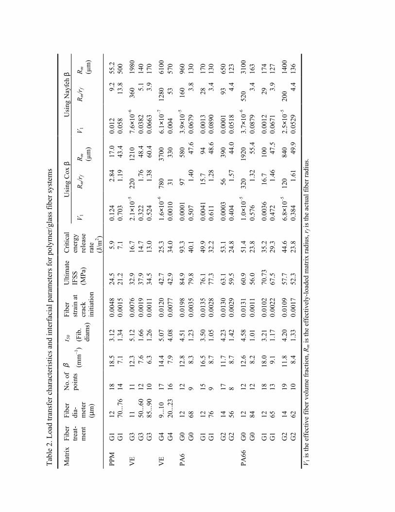
TableÊ2 lists all experimental results for τult and β. For a given matrix and sizing, τult was

found to be independent of fiber diameter. Thus, τult can be suggested as a good material property

13

for characterizing the fiber/matrix interface. We claim it is more realistic than the common

practice of setting the interfacial shear strength to the value of τd determined from the peak load

in the pull-out experiments. Using τult as an interface characterization property, the interface

strengths in the various fibers rank as PA6 ≥ PA66 > VE > PPM. For a constant polymer type,

the sizings rank as G4 > G3 for VE matrix, G0 > G1 > G2 for PA6 matrix, and G1 > G0 ≥ G2 for

PA66 matrix.

The measured β, however, was a function of fiber diameter Ñ it was larger for specimens

with smaller diameter fibers. The literature data on β variations with external conditions are

rather scarce [9, 15, 24], and no information is available about the dependence of β on fiber

radius. Elasticity models consider β to be a well-defined parameter whose value can be calculated

from specimen geometry and elastic properties of the fiber and the matrix (see Eqs. (5) and (6)).

Such calculations of β, however, depend on the effectively-loaded matrix radius, Rm. It has been

shown experimentally that Rm can be considerably smaller than the specimen radius [15, 23].

Similar observations led to the Òrule-of-thumbÓ proposed by Detassis et al. [19] that the Rm/rf

ratio in micromechanical tests should be taken in the region between 2 and 10, independent of the

fiber radius and specimen size; but this assumption appeared to have only limited applicability. It

was shown, in particular, that the β value for a given polymer-fiber system could be altered

substantially as a result of fiber treatment [9, 24]. Furthermore, if the Rm/rf ratio was a constant

then β would be constant; our experiments demonstrated that Rm/rf was neither constant nor

ÒnominalÓ for fibers having different diameters.

A ÒphysicalÓ interpretation of β can be developed by considering its use in analyses of stress

transfer. By experimental observations of fiber-matrix stress transfer (e.g., by Raman

spectroscopy [27]) or from elasticity models of stress transfer [25], the rate of stress transfer

14

between the fiber and matrix can always be described by an exponential function such that the

extent of transfer is proportional to exp(Ðβz). Here z is the distance from any discontinuity such

as a fiber break, a fiber end, or the point where the fiber enters the matrix in a pull-out test. For

such a process, we can define:

trf

502

2= ln

β(9)

The term t50 is the distance required, in dimensionless units of fiber diameters, for the stress

transfer process to be 50% complete. Our results for t50 calculated from the measured βÕs are

given in TableÊ2 and plotted in Fig.Ê3. The stress-transfer distance gets longer as the fiber radius

gets smaller. This result is consistent with elasticity calculations of fiber/matrix stress transfer.

Both numerical and shear-lag calculations for concentric fiber/matrix cylinders show that the

stress transfer distance gets longer as the fiber volume fraction gets smaller [25]. For real

specimens, this volume fraction should refer to an effective volume fraction calculated from the

effectively-loaded matrix radius. Without experiments, it is not possible to tell whether such an

effective fiber volume fraction should decrease or remain the same as the fiber radius gets

smaller, but it is physically unreasonable for it to increase. The experimental results in Fig.Ê3,

show that for this range of fiber radii and this size of matrix droplet, that the stress transfer rate

increases, which implies that the effective fiber volume fraction decreases, and the fiber radius

decreases.

The specimen fiber volume fractions in our experiments calculated using Eq.Ê(8) were always

low (0% < Vf < 0.1%). Although shear-lag analysis does not work when the specimen volume

fraction gets too low, both Eqs.Ê(5) and (6) have interesting low Vf limits that can be compared to

experiments. In fact, both have the same limiting result that can be cast as

15

lim ln lnV f

f

mm f

f r

E

GR r

→= −( )

0 2 21

2β(10)

Interestingly, the only time the Cox β (Eq. (5)) and the Nayfeh β (Eq. (6)) agree is at very low

volume fraction, which is a regime for which shear-lag analysis breaks down [25]. For all volume

fractions at which shear-lag analysis works, the two βÕs are different; the Nayfeh β gives a good

prediction of stress transfer rates while the Cox β is very inaccurate. If Rm is assumed to be

independent of rf, which may not be a good assumption, Eq.Ê(10) predicts that a plot of 1/(β2rf2)

as a function of ln rf should be linear with a slope of ÐEf/(2Gm) while the intercept can be used to

calculate Rm. Such a plot is given in Fig.Ê4 for all experimental results. The plot is roughly linear,

but there is too much scatter and insufficient distribution of fiber radii to confirm a linear relation.

The slope of the Òbest-fitÒ line was Ð78.1. The four matrices had different values of Gm (and

perhaps should not have been on the same plot) giving a range of actual ÐEf/(2Gm) from Ð30.5 to

Ð78.0. Considering the qualitative nature of the analysis, the actual ratio agrees well with the

measured slope. From the intercept of the Òbest fitÓ line, the Rm, which was assumed to be

constant, was 41.7ʵm. Using this result, Rm/rf varied from 0.95 to 8.8. This range is reasonable

[19] but the lower limit is too low. It may not be correct to assume, as done in this interpretation,

that Rm is independent of fiber diameter.

Another route to Rm is to calculate it from the measured values for β and the shear-lag

equations in Eqs.Ê(5) and (6). The results of deducing effective fiber volume fractions, the ratio

Rm/rf, and the effectively-loaded matrix radius Rm using either the Cox β or the Nayfeh β are

given in TableÊ2. Consistent with the stress transfer results in Fig.Ê3, the effective fiber volume

fraction decreased as the fiber radius decreased. The related ratio Rm/rf increased as the fiber

radius decreased. For large fiber diameters (>50ʵm), Rm/rf was in the range 3.4 to 13.8 which is

16

the range commonly assumed for micromechanical tests [19]. For smaller fiber diameters (<30

µm), Rm/rf got much larger. For large fiber diameters (>50 µm), Rm was much smaller than the

specimen dimensions. For smaller fiber diameters (<30 µm), Rm got larger and equaled or

exceeded the specimen dimensions. All these comments refer to results deduced when using the

Nayfeh result for β. It is mathematically possible to deduce the same parameters using the Cox β

(see TableÊ2). Because the Cox β is inaccurate, such calculated dimensions cannot meaningfully

be compared to specimen dimensions.

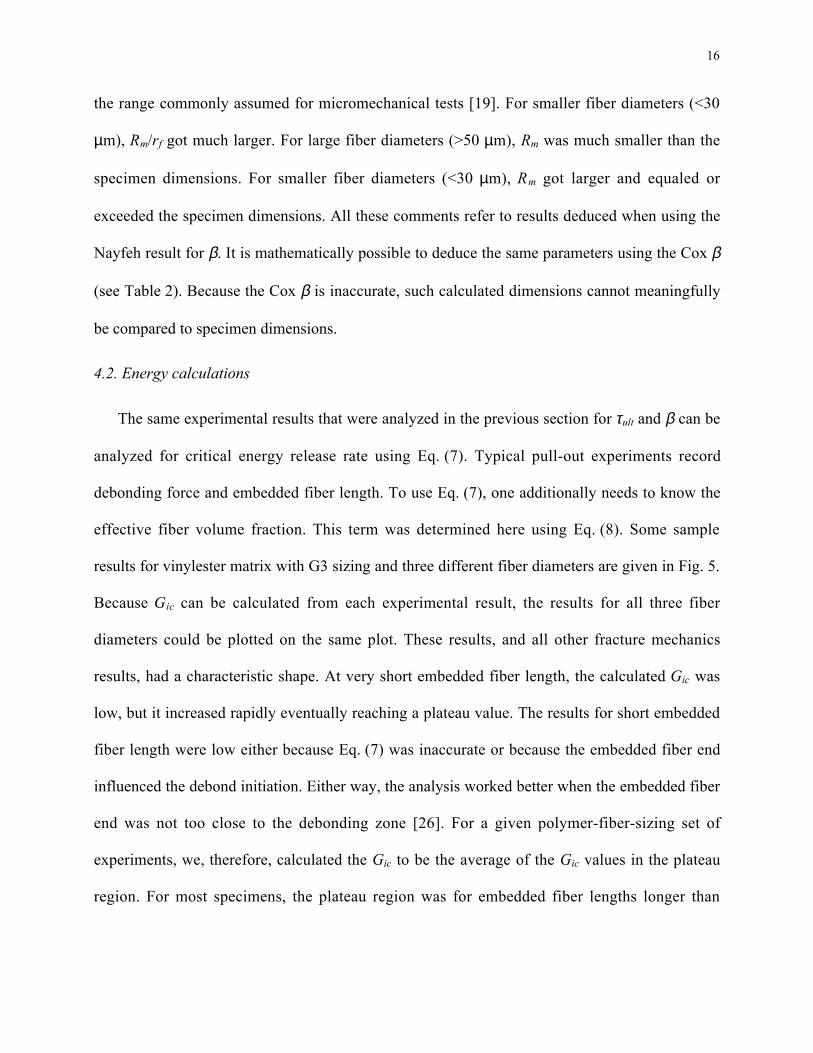
4.2. Energy calculations

The same experimental results that were analyzed in the previous section for τult and β can be

analyzed for critical energy release rate using Eq.Ê(7). Typical pull-out experiments record

debonding force and embedded fiber length. To use Eq.Ê(7), one additionally needs to know the

effective fiber volume fraction. This term was determined here using Eq.Ê(8). Some sample

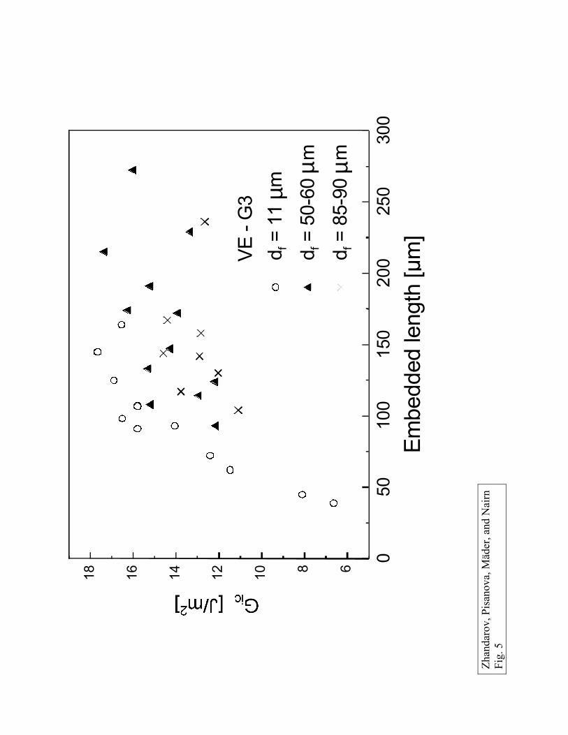
results for vinylester matrix with G3 sizing and three different fiber diameters are given in Fig.Ê5.

Because Gic can be calculated from each experimental result, the results for all three fiber

diameters could be plotted on the same plot. These results, and all other fracture mechanics

results, had a characteristic shape. At very short embedded fiber length, the calculated Gic was

low, but it increased rapidly eventually reaching a plateau value. The results for short embedded

fiber length were low either because Eq.Ê(7) was inaccurate or because the embedded fiber end

influenced the debond initiation. Either way, the analysis worked better when the embedded fiber

end was not too close to the debonding zone [26]. For a given polymer-fiber-sizing set of

experiments, we, therefore, calculated the Gic to be the average of the Gic values in the plateau

region. For most specimens, the plateau region was for embedded fiber lengths longer than

17

100ʵm. For some of the larger radius fibers, the plateau regions required embedded fiber lengths

of 150 to 200ʵm.

The Gic results for all fiber-sizing-matrix systems are listed in TableÊ2. For the PPM and VE

polymers, Gic was nearly independent of fiber diameter. For PA6 and PA66 polymers, however,

Gic depended on fiber diameter; it got smaller as the fiber diameter got larger. Comparing the

different matrices, the interfacial toughness ranked as PA6 > PA66 > VE > PPM. This ranking

agrees with the ranking determined from τult calculations. For a constant polymer type, the

interfacial toughnesses for the sizings rank as G4 > G3 for VE matrix and G0 > G1 = G2 for PA6

matrix. These rankings are nearly the same as the τult rankings with the one exception being that

the τult rankings placed G2 < G1 instead of G2=G1 for the PA6 matrix. Furthermore, the results

for G3 and G4 sizings were also obtained for many other polymer-fiber systems [22]. The Gic

ranking for the PA66 polymer was ambiguous and different than the τult rankings. For small fiber

diameter, the interfacial toughnesses for PA66 ranked as G0 > G2 > G1; for larger fiber

diameters, the interfacial toughnesses of these three sizings were indistinguishable.

4.3 Strength vs. energy calculations

When looking at a single set of experiments with a constant fiber diameter, Gic appears to be

an excellent material property characterizing debonding. For a given polymer-fiber-sizing system,

it was always constant within the plateau region of sufficiently long embedded fibers. When

comparing experiments with different fiber diameters, however, τult may be a better material

property; τult was independent of fiber diameter while Gic sometimes depended on fiber diameter.

For ranking interfacial properties, either material property may be used and they usually gave the

same results. If Gic is used, however, it can only be used to compare results with similar fiber

diameters. For PA66 polymer systems, only the τult results gave a clear ranking. It is possible,

18

however, that the interfacial properties for the three sizings with PA66 polymer were too close to

be clearly distinguished using pull-out experiments.

Most work on crack or debond growth assumes fracture mechanics or energy methods are

more fundamental than strength-based methods. It was somewhat surprising, therefore, that the

strength analysis for τult gave results that were more independent of specimen geometry than the

energy analysis for Gic. A possible explanation is that all our experiments were for initiation of

debonding. Most experimental work in fracture mechanics analyzes growth of existing crack

instead of initiation of a new crack. It is mathematically possible to calculate the energy release

rate for initiation of debonding, but from our experiments, it appears that the conditions to cause

initiation are determined by local stress rather than the initial energy release rate. It would be

interesting to monitor load as a function of debond length and see if the fracture mechanics

methods then give the preferred approach for prediction of debond propagation.

It is important to emphasize that the preferred strength analysis here is not the same as the

strength analyses typically used for pull-out tests. Most strength models are simple average shear

stress models that calculate the average interfacial shear stress at the point of failure using Eq.

(1). The strength analysis here is based on the local or maximum interfacial shear stress. It is more

difficult to determine τult than τd. If β is known for a given system, τult can be determined from τd

using Eq.Ê(3). If β is not known, τult can be determined from the two-parameter fitting process

used here. An advantage of such an analysis is that it additionally leads to an experimental result

for the physically-meaningful β. A possible disadvantage is that the analysis for τult requires

experimental determination of two parameters. Although the Gic calculations gave results that

depended on fiber diameter, one advantage of the energy methods was that these results could be

determined without knowledge of β.

19

5. CONCLUSION

1) Both ultimate IFSS (τult) and critical energy release rate (Gic) are sensitive to fiber treatment

and, thus, characterize the interfacial bond strength.

2) The maximum shear stress failure criterion (τult) gives results that are more independent of

specimen geometry for initiation of debonding than the critical energy release rate (Gic)

criterion. The situation may be different for analysis of propagation of debonding.

3) Analysis of debonding stress as a function of embedded fiber length can be used to deduce

and effective shear-lag parameter, β, which is a measure of the efficiency of load transfer

from the fiber to the matrix. Both the dimensionless βrf and the related Rm/rf ratio are strong

functions of the fiber radius.

4) The single-fiber pull-out test is a useful test for characterizing interfacial properties, but the

data reduction must be done with care. Traditional average shear stress models are probably

too simplistic. Such analyses should be replaced by maximum shear stress models or fracture

mechanics models.

Appendix

The constants required for the fracture mechanics analysis of the pull-out test are defined by

[26]:

CE

V

V EsA

f

m m33

12

1= +

(A-1)

C CV A

V Asm

f33 33

32

0= − (A-2)

)(21

3 mAsD αα −= (A-3)

20

D DV A

V Asm

fT m3 3

3

0= − −( )α α (A-4)

V AV

E

V

E Efm T

T

f m

m

m

m0

1 1 1= − +−

+ +( ) ( )ν ν ν(A-5)

AE

V

V EA

A

f m

m m3 = − +

ν ν. (A-6)

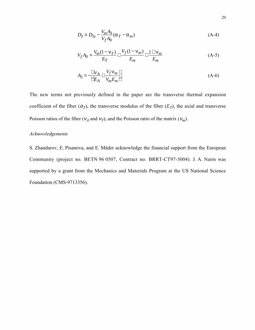
The new terms not previously defined in the paper are the transverse thermal expansion

coefficient of the fiber (αT), the transverse modulus of the fiber (ET), the axial and transverse

Poisson ratios of the fiber (νA and νT), and the Poisson ratio of the matrix (νm).

Acknowledgements

S.ÊZhandarov, E.ÊPisanova, and E.ÊM�der acknowledge the financial support from the European

Community (project no. BETNÊ96Ê0507, Contract no. BRRT-CT97-5004). J.ÊA.ÊNairn was

supported by a grant from the Mechanics and Materials Program at the US National Science

Foundation (CMS-9713356).

21

REFERENCES

1 . M.ÊJ.ÊPitkethly, in: Fiber, Matrix, and Interface Properties, C.ÊJ.ÊSpragg and L.ÊT.ÊDrzal

(Eds.), ASTM STP 1290, pp.Ê34Ð46. ASTM, Philadelphia (1996).

2. I.ÊVerpoest, M.ÊDesaeger and R.ÊKeunings, in Controlled Interfaces in Composite Materials,

H.ÊIshida (Ed.), pp. 653Ð666. Elsevier, New York (1990).

3. M.ÊR.ÊPiggott, Composites Sci. Technol. 57, 965Ð974 (1997).

4 . M.ÊJ. Pitkethly, J.ÊP. Favre, U. Gaur, J. Jakubowski, S.ÊF. Mudrich, D.ÊL. Caldwell,

L.ÊT.ÊDrzal, M. Nardin, H.ÊD. Wagner, L. DiLandro, A. Hampe, J.ÊP. Armistead,

M.ÊDesaeger and I.ÊVerpoest, Composites Sci. Technol. 48, 205Ð214 (1993).

5. Yu.ÊA. Gorbatkina, Adhesive Strength of FibreÐPolymer Systems. Ellis Horwood, New York

(1992).

6. G.ÊD�sarmot and J.-P.ÊFavre, Composites Sci. Technol. 42, 151 (1997).

7. M.ÊJ.ÊPitkethly and J.ÊB.ÊDoble, in Controlled Interfaces in Composite Materials, H.ÊIshida

(Ed.), pp. 809Ð818. Elsevier, New York (1990).

8. S.ÊF. Zhandarov and E.ÊV.ÊPisanova, Composites Sci. Technol. 57, 957Ð964 (1997).

9. N.ÊTakeda, D.ÊY.ÊSong, K.ÊNakata and T.ÊShioya, Composite Interfaces 2, 143Ð155 (1994).

10. R.ÊJ.ÊScheer and J.ÊA.ÊNairn, J.ÊAdhesion 53, 45 (1995).

11. C.-H.ÊLiu and J.ÊA.ÊNairn, Int. J. Adhesion and Adhesives 19, 59Ð70 (1999).

12. M.ÊR.ÊPiggott, Carbon 27, 657 (1989).

13. H.ÊL.ÊCox, Br.ÊJ.ÊAppl. Phys. 3, 72 (1952).

14. A.ÊH.ÊNayfeh, Fibre Sci. Technol. 10, 195Ð209 (1977).

15. M.ÊShioya, E.ÊMikami and T.ÊKikutani, Composite Interfaces 4, 429Ð445 (1997).

22

16. A.ÊS.ÊNielsen and R.ÊPyrz, in ICCM-12: 12th Int. Conf. on Composite Mater. Paris, France,

5th-9th July 1999. Extended Abstracts, p.224. Paris, 1999.

17. M.ÊC.ÊAndrews, R.ÊJ.ÊYoung and J.ÊMahy, Composite Interfaces 2, 433Ð456 (1994).

18. C.ÊGaliotis, Composites Sci. Technol. 42, 125 (1991).

19. M.ÊDetassis, E.ÊFrydman, D.ÊVrieling, X.-F.ÊZhou, H.ÊD.ÊWagner and J.ÊA.ÊNairn, Composites

Part A 27A, 769Ð773 (1996).

20. E.ÊM�der, K.ÊGrundke, H.-J.ÊJacobasch and G.ÊWachinger, Composites 25, 739Ð744 (1994).

2 1 . L.ÊB.ÊGreszczuk, in Interfaces in Composites, ASTM STP 452, pp. 42Ð58. ASTM,

Philadelphia (1969).

22. S.ÊZhandarov, E.ÊPisanova and B.ÊLauke, Composite Interfaces 5, 387Ð404 (1998).

23. S.ÊZhandarov, E.ÊPisanova and E.ÊM�der, Composite Interfaces, submitted (2000).

24. E.ÊPisanova and E.ÊM�der, J.ÊAdhesion Sci. Technol. 14, 415Ð436 (2000).

25. J.ÊA.ÊNairn, Mech. Materials 26, 63Ð80 (1997).

26. J. A. Nairn, Advanced Composite Letters, submitted (2000).

27. R. J. Young and M. C. Andrews, Mater. Sci. Engng A184, 197–205 (1994).

Tab

le 1

. Mec

hani

cal a

nd th

erm

al p

rope

rtie

s of

the

fibe

r an

d m

atri

ces

used

in th

is s

tudy

Prop

erty

E-g

lass

Mod

ifie

d po

lypr

opyl

ene

(PPM

)

Vin

yles

ter

resi

n

(VE

)

Poly

amid

e 6

(PA

6)

Poly

amid

e 6,

6

(PA

66)

Ten

sile

mod

ulus

(E

f or

Em)

(GPa

)75

1.3

2.5

2.8

3.2

Pois

sonÕ

s ra

tio (

ν f o

r ν m

)0.

170.

350.

340.

380.

30

Shea

r m

odul

us (

Gf o

r G

m)

(GPa

)32

0.48

0.93

1.01

1.23

Axi

al C

TE

(α f

orα

m)

(ppm

/¡C

)5

150

6565

81

Tra

nsve

rse

CT

E (

α T)

(ppm

/¡C

)5

150

6565

81

Stre

ss-f

ree

tem

pera

ture

(¡C

)Ñ

<25

7076

78

Tab

le 2

. Loa

d tr

ansf

er c

hara

cter

istic

s an

d in

terf

acia

l par

amet

ers

for

poly

mer

/gla

ss f

iber

sys

tem

s

Usi

ng C

ox β

Usi

ng N

ayfe

h β

Mat

rix

Fibe

rtr

eat-

men

t

Fibe

rdi

a-m

eter

(µm

)

No.

of

poin

tsβ (m

mÐ1

)

t 50

(Fib

.di

ams)

Fibe

rst

rain

at

crac

kin

itiat

ion

Ulti

mat

eIF

SS(M

Pa)

Cri

tical

ener

gyre

leas

era

te(J

/m2 )

V1

Rm/r

fR

m

(µm

)V

1R

m/r

fR

m

(µm

)

PPM

G1

1218

18.5

3.12

0.00

4824

.5 5

.90.

124

2

.84

17.

00.

012

9.2

55.2

G1

70...

7614

7.1

1.34

0.00

1521

.2 7

.10.

703

1

.19

43.

40.

058

1

3.8

500

VE

G3

1111

12.3

5.12

0.00

7632

.916

.72.

1×10

Ð522

012

107.

6×10

Ð6 3

6019

80G

350

...60

12 7

.61.

660.

0019

37.9

14.7

0.32

2

1.7

6 4

8.4

0.03

82

5.

114

0G

385

...90

10 6

.31.

260.

0011

34.5

13.0

0.52

4

1.3

8 6

0.4

0.06

63

3.

917

0

VE

G4

9...1

017

14.4

5.07

0.01

2042

.725

.31.

6×10

Ð678

037

006.

1×10

Ð712

8061

00G

420

...23

16 7

.94.

080.

0077

42.9

34.0

0.00

10 3

1 3

300.

004

5

357

0

PA6

G0

1212

12.8

4.51

0.01

9884

.993

.30.

0001

97

580

3.9×

10Ð5

160

960

G0

689

8.3

1.23

0.00

3579

.840

.10.

507

1

.40

4

7.6

0.06

79

3.

813

0

G1

1215

16.5

3.50

0.01

3576

.149

.90.

0041

15.

7

94

0.00

13

28

170

G1

769

8.7

1.05

0.00

2877

.332

.20.

611

1

.28

4

8.6

0.08

90

3.

413

0

G2

1417

11.7

4.23

0.01

3063

.153

.10.

0003

56

390

0.00

01

93

650

G2

568

8.7

1.42

0.00

2959

.524

.80.

404

1

.57

4

4.0

0.05

18

4.

412

3

PA66

G0

1212

12.6

4.58

0.01

3160

.951

.41.

0×10

Ð532

019

203.

7×10

Ð652

031

00G

084

12 8

.21.

010.

0011

56.0

23.8

0.57

6

1.3

2

55.

40.

0879

3.4

163

G1

1218

18.0

3.21

0.01

0270

.73

35.2

0.00

36 1

6.7

100

0.00

12

29

174

G1

6513

9.1

1.17

0.00

2267

.529

.30.

472

1

.46

4

7.5

0.06

71

3.

912

7

G2

1419

11.8

4.20

0.01

0957

.744

.66.

8×10

Ð512

0 8

402.

5×10

Ð520

014

00G

262

10 8

.41.

330.

0017

52.3

23.8

0.38

4

1.6

1

49.

90.

0529

4.4

136

V1

is th

e ef

fect

ive

fibe

r vo

lum

e fr

actio

n, R

m is

the

effe

ctiv

ely-

load

ed m

atri

x ra

dius

, rf i

s th

e ac

tual

fib

er r

adiu

s.

FIGURE CAPTIONS

Fig.Ê1.ÊTypical force-displacement curve from a pull-out test. The debonding was assumed to

initiate at the debond force, Fd, which corresponds to the knee in the force-displacement

curve. Fd was always smaller than the maximum force value recorded during the test.

Fig.Ê2.ÊDebond shear stress (τd) as a function of embedded fiber length for glass fibers with G3

sizing embedded in vinylester resin. The solid line is the best fit to Eq.Ê(3). The fiber

diameters were 11ʵm (a), 50Ð60ʵm (b) and 85Ð90ʵm (c).

Fig.Ê3.ÊThe distance required for the stress transfer process to be 50% complete (in dimensionless

units of fiber diameters from Eq. (9)) vs the fiber radius (for all experimental results).

Fig.Ê4.ÊExperimental results for the dimensionless term (βrf)Ð2 as a function of lnÊrf (when rf is in

µm). For details see text.

Fig.Ê5.ÊTypical plot of the critical energy release rate (Gic) as a function of the embedded length

for glass fibers with G3 sizing embedded in vinylester resin. Gic was calculated using the

long-fiber analysis in Eq. (7).

05

1015

2025

300.00

0.05

0.10

0.15

0.20

PA6-G0

d f=12µm

u d

Fd

Displacement[µm]

Zha

ndar

ov, P

isan

ova,

M�d

er, a

nd N

airn

Fig.

1

0.00

0.05

0.10

0.15

0.20

05101520253035

VE-G3

d f=11µm

β=12344m-1

Embeddedlength[mm]

Zha

ndar

ov, P

isan

ova,

M�d

er, a

nd N

airn

Fig.

2A

0.00

0.05

0.10

0.15

0.20

0.25

0.30

0510152025303540

VE-G3

d f=50-60µm

β=7614m-1

Embeddedlength[mm]

Zha

ndar

ov, P

isan

ova,

M�d

er, a

nd N

airn

Fig.

2B

0.00

0.05

0.10

0.15

0.20

0.25

0.30

05101520253035

VE-G3

d f=85-90µm

β=6342m-1

Embeddedlength[ mm]

Zha

ndar

ov, P

isan

ova,

M�d

er, a

nd N

airn

Fig.

2C

010

2030

4050

0123456

Fiberradius[µm]

Zha

ndar

ov, P

isan

ova,

M�d

er, a

nd N

airn

Fig.

3

1.0

1.5

2.0

2.5

3.0

3.5

4.0

050100

150

200

250

ln( Fiberradius[µm])

Zha

ndar

ov, P

isan

ova,

M�d

er, a

nd N

airn

Fig.

4

ength[µm]

050

100

150

200

250

300

68

1012141618

VE-G3

d f=11

µmd f=50-60

µmd f=85-90

µm

Embeddedl

Zha

ndar

ov, P

isan

ova,

M�d

er, a

nd N

airn

Fig.

5