investigation of intraoral mechanical effects on sensory sensations
TRANSCRIPT
Technische Universitat Munchen
Lehrstuhl fur Fluidmechanik und Prozessautomation
Investigation of
Intraoral Mechanical Effects on
Sensory Sensations and their
Contribution to Mouthfeel
Katrin Mathmann
Vollstandiger Abdruck der von der Fakultat Wissenschaftszentrum Weihenstephan fur
Ernahrung, Landnutzung und Umwelt der Technischen Universitat Munchen zur
Erlangung des akademischen Grades eines
Doktor-Ingenieurs (Dr.-Ing.)
genehmigten Dissertation.
Vorsitzender: Univ.-Prof. Dr. H.-Chr. Langowski
Prufer der Dissertation: 1. Univ.-Prof. Dr. A. Delgado
(Friedrich-Alexander-Universitat Erlangen-Nurnberg)
2. Univ.-Prof. Dr. Th. Becker
3. Univ.-Prof. Dr. H. Ulbrich
Die Dissertation wurde am 21.12.2010 bei der Technischen Universitat Munchen eingereicht
und durch die Fakultat Wissenschaftszentrum Weihenstephan fur Ernahrung, Landnutzung
und Umwelt am 03.06.2011 angenommen.

there is
no conception in man’s mind
which hath not at first,
totally or by parts,
been begotten upon
the organs of sense
Thomas Hobbes
Leviathan, 1651

Abstract
The rheology of food capable of flowing has a major impact on human texture perception.
To understand intraoral fluid flow greater, a series of tongue-palate models designed to study
deglutition from the fluid-mechanical point of view have been presented. Via the theory of
lubrication three new analytical models have been introduced. In particular, the model of a
sphere in a hemisphere has given superior results compared to the established, but simpler,
model of Stefan. A more complex geometry, treated numerically, confirmed these findings.
The fluid-mechanical quantities obtained from the models employed for the first time give
new insights into mechanoreception in the human oral cavity.
Die Rheologie eines fließfahigen Lebensmittels besitzt einen großen Einfluss auf die humane
Texturwahrnehmung. Zum besseren Verstandnis des intraoralen Fließverhaltens erfolgte die
Gegenuberstellung unterschiedlicher Zunge-Gaumen-Modelle, die den Schluckvorgang aus
stromungsmechanischer Sicht nachstellen. Die Schmierfilmtheorie ermoglichte die analytis-
che Berechnung drei neuer Modelle. Insbesondere das Modell einer Kugel in einer Halbkugel
lieferte Ergebnisse, die dem etablierten, aber einfacheren Modell nach Stefan uberlegen sind.
Numerische Berechnungen in einer komplexeren Geometrie bestatigten diese Ergebnisse. Die
aus den erstmalig eingesetzten Modellen gewonnenen Stromungsgroßen lassen neue Erken-
ntnisse hinsichtlich der Mechanorezeption in der menschlichen Mundhohle zu.

Contents
List of Symbols v
1 Introduction 1
1.1 Motivation for Studying Texture . . . . . . . . . . . . . . . . . . . . . . . . . 2
1.2 Aim of the Current Thesis . . . . . . . . . . . . . . . . . . . . . . . . . . . . 3
1.3 Approach . . . . . . . . . . . . . . . . . . . . . . . . . . . . . . . . . . . . . 4
2 State of the Art 7
2.1 Selected Aspects of Rheology . . . . . . . . . . . . . . . . . . . . . . . . . . 8
2.2 Fundamentals and Physics of Sensing . . . . . . . . . . . . . . . . . . . . . . 9
2.2.1 Definition of Food Texture and Mouthfeel . . . . . . . . . . . . . . . 10
2.2.2 Impacts on Perceived Texture . . . . . . . . . . . . . . . . . . . . . . 12
2.2.3 Oral Food Texture Evaluation and Terminology . . . . . . . . . . . . 15
2.2.4 Oral Shear Stresses and Shear Rates . . . . . . . . . . . . . . . . . . 18
2.2.5 Numerical Simulations . . . . . . . . . . . . . . . . . . . . . . . . . . 23
2.3 Physiology of Texture Perception . . . . . . . . . . . . . . . . . . . . . . . . 27
2.3.1 Classification of the Mechanoreceptors . . . . . . . . . . . . . . . . . 28
2.3.2 Impulse-Discharge Patterns . . . . . . . . . . . . . . . . . . . . . . . 29
i
ii CONTENTS
2.3.3 Occurrence of Mechanoreceptors . . . . . . . . . . . . . . . . . . . . . 31
2.3.4 Comparison between Hand and Tongue . . . . . . . . . . . . . . . . . 32
2.3.5 Histological Classification of the End Organs . . . . . . . . . . . . . . 33
2.3.6 Sensitivity . . . . . . . . . . . . . . . . . . . . . . . . . . . . . . . . . 34
3 Analytical Models and Numerical Methods 37
3.1 Geometrical Model of the Oral Cavity . . . . . . . . . . . . . . . . . . . . . 38
3.2 Basic Equations of Fluid Flow . . . . . . . . . . . . . . . . . . . . . . . . . . 40
3.3 Theory of Lubrication . . . . . . . . . . . . . . . . . . . . . . . . . . . . . . 44
3.3.1 Reynolds Equation . . . . . . . . . . . . . . . . . . . . . . . . . . . 45
3.3.2 Squeezing Flow . . . . . . . . . . . . . . . . . . . . . . . . . . . . . . 50
3.3.3 Plane Circular Parallel Plates - Stefan Equation . . . . . . . . . . . 51
3.3.4 Plane Elliptic Parallel Plates . . . . . . . . . . . . . . . . . . . . . . . 57
3.3.5 Plane and Curved Circular Parallel Plates . . . . . . . . . . . . . . . 61
3.3.6 Sphere in a Hemisphere . . . . . . . . . . . . . . . . . . . . . . . . . 64
3.3.7 Summary of Analytical Equations . . . . . . . . . . . . . . . . . . . . 69
3.4 Numerical Simulations . . . . . . . . . . . . . . . . . . . . . . . . . . . . . . 69
3.4.1 Procedure of a CFD Analysis . . . . . . . . . . . . . . . . . . . . . . 71
3.4.2 Discretization Methods . . . . . . . . . . . . . . . . . . . . . . . . . . 72
3.4.3 Types of Grids . . . . . . . . . . . . . . . . . . . . . . . . . . . . . . 73
3.4.4 Software . . . . . . . . . . . . . . . . . . . . . . . . . . . . . . . . . . 73
3.4.5 Introduction of the Geometrical Model . . . . . . . . . . . . . . . . . 76
CONTENTS iii
4 Results and Discussion 79
4.1 Rheological Measurements and Fittings . . . . . . . . . . . . . . . . . . . . . 80
4.2 Theory of Lubrication . . . . . . . . . . . . . . . . . . . . . . . . . . . . . . 85
4.2.1 Plane Circular Parallel Plates - Stefan Equation . . . . . . . . . . . 85
4.2.2 Plane Elliptic Parallel Plates . . . . . . . . . . . . . . . . . . . . . . . 90
4.2.3 Plane and Curved Circular Parallel Plates . . . . . . . . . . . . . . . 95
4.2.4 Sphere in a Hemisphere . . . . . . . . . . . . . . . . . . . . . . . . . 99
4.2.5 Conclusion . . . . . . . . . . . . . . . . . . . . . . . . . . . . . . . . . 108
4.3 Numerical Simulations . . . . . . . . . . . . . . . . . . . . . . . . . . . . . . 110
4.3.1 Pressures . . . . . . . . . . . . . . . . . . . . . . . . . . . . . . . . . 112
4.3.2 Velocities . . . . . . . . . . . . . . . . . . . . . . . . . . . . . . . . . 118
4.3.3 Shear Rates . . . . . . . . . . . . . . . . . . . . . . . . . . . . . . . . 123
4.3.4 Viscosities . . . . . . . . . . . . . . . . . . . . . . . . . . . . . . . . . 128
4.3.5 Shear Stresses . . . . . . . . . . . . . . . . . . . . . . . . . . . . . . . 131
4.4 Summary of Analytical and Numerical Findings . . . . . . . . . . . . . . . . 133
5 Conclusions 135
5.1 Analytical Models . . . . . . . . . . . . . . . . . . . . . . . . . . . . . . . . . 136
5.2 Numerical Models . . . . . . . . . . . . . . . . . . . . . . . . . . . . . . . . . 139
5.3 Mechanoreception . . . . . . . . . . . . . . . . . . . . . . . . . . . . . . . . . 142
5.4 Outlook . . . . . . . . . . . . . . . . . . . . . . . . . . . . . . . . . . . . . . 142
Bibliography 145
Appendices 157

iv CONTENTS
A Peer-reviewed Papers 157
B Calculation of the Arc of Circle 159
C Code nonNewtonianIcoDyMFoam 161
List of Symbols
There are three different coordinate systems, which are used for the derivation of the different
fluid-mechanical models, namely the Cartesian coordinate system (x, y, z), the cylindrical
coordinate system (r, φ, z) and the spherical coordinate system (r, φ, θ). The fluid mechan-
ical quantities that are subscribed with these coordinates stand for the components in those
directions. Tensor index notation is used for the subscripts i and j. These run from 1 to 3
and represent the coordinates of the different systems.
Latin
A area
a semi-major axis of the ellipse
b semi-minor axis of the ellipse
C1, C2 constants of integration
c clearance
ce ratio of the ellipse axes ba
D shear rate
ez eccentricity
F external force required to drive the different geometries together
fc constant used in the ansatz function for plane elliptic parallel plates
g gravity constant
h film thickness of a fluid film
v

vi LIST OF SYMBOLS
h0 minimal film thickness (1 mm)
m consistency factor
n flow-behavior index
p pressure
p0 ambient pressure
r coordinate in radial direction
R general plate radius or sphere radius (35 mm), respectively
R1 radius of the key points in the frontal plane
R2 radius of the key points in the sagittal plane
Ra1 minimal averaged radius on the basis of the arc of the circle in the frontal plane
(26 mm)
Ra2 maximal averaged radius on the basis of the arc of the circle in the sagittal
plane (35 mm)
Rp1 minimal averaged radius in the transverse projection plane (18 mm)
Rp2 maximal averaged radius in the transverse projection plane (29 mm)
t time
u velocity
umag magnitude of velocity
u average velocity
V volume flow rate
vp uniform velocity of the moving geometry part (1 cm/s)
w0 velocity of the lower movable surface used in the derivation of the Reynolds
equation
wh velocity of the upper movable surface used in the derivation of the Reynolds
equation
LIST OF SYMBOLS vii
Greek
α constant in the Cross law associated with the rupture of linkages
β curvature parameter in the plane and curved circular parallel plate model
γ shear rate
η dynamic viscosity
η∞ dynamic infinite-shear viscosity
η0 dynamic zero-shear viscosity
ν kinematic viscosity
ν∞ kinematic infinite-shear viscosity
ν0 kinematic zero-shear viscosity
ρ density of the fluid
σ shear stress
σ0 yield stress
τij viscous stress tensor
τzr shear-stress component perpendicular to the main fluid-flow direction r for cylindri-
cal coordinates
τzz normal stress component in z-direction
ψ angle by which hemispherical shell can be tilted
ω angular velocity

Chapter 1
Introduction
Foods are evaluated using four principal parameters. These are appearance, flavor, texture
and nutrition. Of these, only the last parameter, nutrition, cannot be perceived by the
human senses. The other attributes are perceived by the five senses - sight, hearing, smell,
taste, and touch.
Appearance is sensed optically with the eyes. Flavor is a matter of the chemical senses.
They perceive gustatory and olfactory stimuli by means of the tongue and nose. Texture
is a multifaceted parameter mainly sensed by the tactile and kinesthetic senses. Here, the
tactile sense refers to touch, the kinesthetic sense to joint position. Moreover, vision and
hearing are involved in the process of texture perception.
The process of texture perception is a sequence of several impressions. Thinking of an
apple as an example, we first evaluate its texture visually. We look at shape and color and
check if the apple is undamaged. Afterwards, we bite into it while listening to the quality of
the crunching sound. Last but not least, we start to chew the apple and therefore employ
our tactile and kinesthetic senses in order to evaluate the texture from a mechanical point
of view. Our brain combines all these sensations and makes a decision about the quality of
the apple.
This sequence of steps takes place subconsciously. We will only pay attention to them
if the texture of the apple is different from our expectation. Nevertheless, the food will be
1
2 CHAPTER 1. INTRODUCTION
rejected if the expectations are not met. For that reason, the food industry is more and
more interested in designing perfect textures to keep customers. Hence, food texture and
texture perception are worth a closer glance.
1.1 Motivation for Studying Texture
Texture perception and mouthfeel are sensory variables that only came into the focus of
research in the 1960s, whereas flavor has been studied for a much longer time. As a result,
these concepts still need basic understanding and further clarification. The early attempts
of research in this field consisted of work establishing terminology, definitions and concepts
of food texture as well as determining the different factors that affect perception. Soon it
became obvious that texture is a collective term with many facets. One mode of sensing
is not enough to collect a comprehensive impression of all the textural information of food.
Nevertheless, there is a consensus in the literature that texture and mouthfeel are dominated
by mechanical attributes. These attributes cover a wide range from hardness-related to
viscosity-related terms. Although concentrating only on mechanical stimuli, it is obvious
that the description of texture exhibits much more complexity than flavor, which can be
related to individual chemical compounds.
Due to this complexity, a reliable method to describe mouthfeel quantitatively by means
of physical measurements is currently missing. Nevertheless, finding such a method is the
desired and ultimate aim of food-texture research. Peleg (1993) aptly states that “if a
‘perceived texture’ is, indeed, a sensory response to ... objective mechanical attributes, then
the creation of a ‘tailored texture’ is a realistic possibility”. This vision of food that is not
only harmonious in flavor but also blends well with its texture spurs on food scientists all
over the world.
One big challenge is the diversity of foodstuffs. Only taking into account those foods
that are capable of flowing slightly reduces the huge variety of foods. There still remains a
widespread collection of food that can obviously be distinguished by its fluid-flow behavior.
1.2. AIM OF THE CURRENT THESIS 3
Every consumer knows from daily-life breakfast experience that the contents of a coffee cup
spill widely over the whole table after tipping the cup over while honey is difficult to spread
properly on toast. These different behaviors also occur in the oral cavity. They are one
aspect by which the consumer judges texture and decides about individual preferences. One
branch of research on food texture aims at expressing these experiences with differently
behaving foods mathematically. The resulting mathematical models should act as a basis
for understanding the food-consumer interaction objectively.
The most important terms describing texture and mouthfeel for foods capable of flowing
are viscosity-related terms. Hence, some studies dealing with sensory evaluations of food
thickness are available as well as some others discussing the shear rates and stresses that
occur in the mouth. So far the fluid mechanical quantities occurring in the mouth have been
quantified by both experimental approaches and calculations. These quantities are said to
be detected by the oral mechanoreceptors and give an idea about the mechanically-induced
mouthfeel sensations. For this reason, one of the aims of food-texture research is to close
the existing gap between instrumental and human sensory measurements.
1.2 Aim of the Current Thesis
The current thesis concentrates on the calculation of fluid flow in several oral model systems.
The models introduced increase in complexity. The simple models are solved analytically
by means of the theory of lubrication. The advanced models, with a geometry that is based
on dentist replicas, require numerical treatment. Evaluating the results of these analytical
fluid-mechanical investigations gives good estimates of the order of magnitude of the different
fluid-mechanical quantities.
The analytical calculations help to estimate the influence of different geometries on fluid
flow. The numerical simulations visualize vector fields of fluid-flow variables in a more
complex geometry. Moreover, a model including a non-Newtonian fluid is introduced. This
is interesting as most foodstuffs capable of flowing are non-Newtonian fluids.
4 CHAPTER 1. INTRODUCTION
The current thesis reviews literature concerning the concept of texture, existing models
of the oral cavity, and the fundamentals of mechanoreception. Subsequently, the different
models of the oral cavity are introduced and the results of the calculations are discussed and
compared. The final validation of each flow variable is accomplished by means of comparison
to existing literature values. Hence, the present thesis provides a more detailed insight into
the fluid-mechanical processes in the oral cavity than ever before.
1.3 Approach
The analytical approaches that have been employed so far all relate to a well-known tongue-
palate model system consisting of two plane circular parallel plates. This system can roughly
mimic the squeezing flow that occurs during deglutition (swallowing) and gives an idea of
the expected order of magnitude of fluid-mechanical quantities. Nevertheless, this analytical
approach lacks a geometry that is closer to reality.
The in-mouth models employed in the current thesis enable the investigation of fluid-flow
processes in the oral cavity that accompany consumption. Two approaches are introduced, an
analytical one and a numerical one. Concerning the analytical one, first of all the established
geometry of two plane circular parallel plates is introduced. This geometry is well described
concerning all fluid-mechanical quantities as it is often used as a reference.
The established model is compared to geometries that consider different aspects of the
real oral cavity. The first geometry for comparison consists of two plane elliptical parallel
plates. The pressures and the force required to drive the geometry together have been known
for a long period. Additionally, the current thesis determines velocities, shear rates and shear
stresses. The same is performed for a second geometry consisting of a plane and a curved
circular parallel plate. Finally, the analytically solvable model of a sphere in a hemisphere
is derived from a general approach to lubrication.
The numerical approach employs a geometrical model that is built on average values
of oral cavities. The flow of fluids featuring different viscosities is calculated. Here, three
1.3. APPROACH 5
different low viscosities are employed to investigate the effect of small viscosity changes on
the distribution of the fluid-mechanical quantities. Additionally, one fluid with a higher
viscosity that represents both vegetable oils and the apparent viscosity of yogurt is used.
Lastly, a non-Newtonian fluid fitted with the Cross law is implemented in the numerical
calculation. This approach of implementing a different flow-curve characteristic is reasonable
as most foodstuffs exhibit non-Newtonian fluid flow behavior. This makes the comparison of
Newtonian and non-Newtonian results essential as the differences are likely to have a great
effect on texture perception.
All the different approaches reveal mechanical stimuli that occur due to the movement
of the tongue during deglutition. These stimuli are detected dynamically by the human
mechanoreceptors in the oral cavity. The tactile sensation is then transmitted to the human
brain. For this reason, this thesis establishes a link to perception. Knowledge of what the
mechanoreceptors detect and magnitudes of different physical quantities of fluids within the
oral cavity means a novel understanding of the food-consumer interaction.

Chapter 2
State of the Art
This chapter begins with a short introduction to the idea of rheology. This is necessary as the
term is frequently used when dealing with texture and mouthfeel. Thereafter, the sensory,
physical and physiological fundamentals of texture perception are presented. Starting with
the concept of texture, definitions, influences on perception and terminology of mouthfeel
attributes are outlined. In this context, it will be shown that viscosity is the most dominant
mouthfeel attribute for food capable of flowing. Therefore, it becomes obvious why the
current investigation concentrates on models that mimic the squeezing flow in the oral cavity.
Furthermore, the shear stresses and rates occurring in the mouth that result from ex-
perimental investigations and theoretical considerations are discussed. Previous numerical
simulations of deglutition have focused on the pharynx and the esophagus as these organs in
particular have attracted the attention of medical scientists so far. Their primary aim was
the understanding of dysphagia in order to develop a cure for this condition. Nevertheless,
numerical models of the oral cavity are rare.
The chapter ends with a short introduction to the physiology of perception. Mechanore-
ceptors are referred to in many papers dealing with texture perception. Hence, their mor-
phology and functionality are illustrated. An improved knowledge of mechanoreceptors is
the basis for understanding the signal transmission from the food through the oral tissues
to the brain, which evaluates the sensations.
7
8 CHAPTER 2. STATE OF THE ART
2.1 Selected Aspects of Rheology
Rheology deals with the deformation and flow of matter in response to an applied stress or
strain. The reaction of matter caused by the applied stress or strain is used to characterize
rheological behavior (Steffe, 1996). In principle, rheological characteristics can be classified
into Newtonian and non-Newtonian behavior. Newtonian fluids feature a constant viscosity,
while the viscosity of non-Newtonian fluids depends on the applied shear rate. Typical
examples of Newtonian fluid-flow behavior are water, vegetable oils and honey. In contrast,
most foods show non-Newtonian behavior (Steffe, 1996, Bourne, 2002).
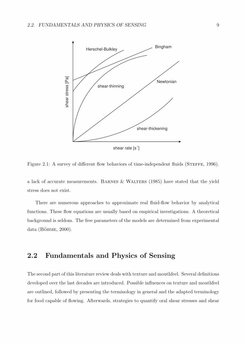
Rheologists distinguish between some major material behaviors. Figure 2.1 introduces
the time-independent characteristics by plotting shear stress σ versus shear rate γ (Steffe,
1996). Time-dependent models are not considered in the current study due to their com-
plexity. Newtonian fluids exhibit a direct proportionality between shear stress σ and shear
rate γ. The slope of the flow curve is the dynamic viscosity η.
Non-Newtonian materials do not feature this direct linear proportionality. However, the
local quotient σγis often used to define an apparent viscosity η. If the apparent viscosity η
decreases with an increasing shear rate γ, the material is said to exhibit shear-thinning
behavior. An example of this kind of fluid-flow behavior is orange-juice concentrate. The
opposite case, where the apparent viscosity η increases with an increasing shear rate γ, is
known as shear-thickening behavior. This behavior can be observed in the case of starch
solutions (Steffe, 1996).
Both, the Bingham and the Herschel-Bulkley fluids are said to require a minimum
applied stress to make them deform and flow. This stress is called the yield stress σ0. Below
this yield stress, the material behaves like a solid. Its value can be read off the y-axis
intercept. Above this yield stress, when the matter flows, the curves can show a linear
proportionality between shear stress σ and shear rate γ once again (Bingham) or a shear-
thinning characteristic (Herschel-Bulkley). Tomato paste is said to comply with the
Bingham model, ketchup with the Herschel-Bulkley model (Steffe, 1996). However,
the yield-stress concept has been criticized as being an idealization, which has arisen due to
2.2. FUNDAMENTALS AND PHYSICS OF SENSING 9
Herschel-BulkleyBingham
shear-thinningNewtonian
shear-thickening
shear rate [s ]-1
sh
ea
r str
ess [
Pa
]
Figure 2.1: A survey of different flow behaviors of time-independent fluids (Steffe, 1996).
a lack of accurate measurements. Barnes & Walters (1985) have stated that the yield
stress does not exist.
There are numerous approaches to approximate real fluid-flow behavior by analytical
functions. These flow equations are usually based on empirical investigations. A theoretical
background is seldom. The free parameters of the models are determined from experimental
data (Bohme, 2000).
2.2 Fundamentals and Physics of Sensing
The second part of this literature review deals with texture and mouthfeel. Several definitions
developed over the last decades are introduced. Possible influences on texture and mouthfeel
are outlined, followed by presenting the terminology in general and the adapted terminology
for food capable of flowing. Afterwards, strategies to quantify oral shear stresses and shear
10 CHAPTER 2. STATE OF THE ART
rates are outlined. The section closes with a summary of numerical studies that have been
employed previously in order to visualize the process of swallowing.
2.2.1 Definition of Food Texture and Mouthfeel
Scientists have long been aware of the importance of flavor for consumer acceptance. How-
ever, the multi-parameter attribute texture has only attracted attention since the 1960s
(Szczesniak, 2002). There are several definitions of food texture presented in the litera-
ture. Some of them take only one kind of foodstuff into consideration whereas others are
more general.
In one of her early publications Szczesniak (1963) defined that texture can be “consid-
ered as the composite of the structural elements of food and the manner in which it registers
with physiological senses”. A few years later, Muller (1969) regarded the concept of texture
as confusing because it relates to both a physical and a perceived property. He suggested a
separation in the terms “rheology” and “hapaesthesis” instead. According to this concept,
rheology is measured objectively in SI units, while hapaesthesis is recorded by means of
statistical investigations.
Although Szczesniak tried to define texture in 1963, she admitted in the same paper
that a clearer appreciation of the concept must be worked out. She recognized that “a
rigorous definition of texture will have to await a better understanding of the basic princi-
ples involved, especially those concerned with rheological or mechanical properties of food”.
Following her, these early definitions have been updated continuously.
Texture was much debated in the 1970s. Sherman (1970) refined the definition of
Szczesniak (1963) saying that texture is “the composite of those properties (attributes)
which arise from the structural elements of food and the manner in which it registers with
physiological senses”. With this definition he wanted to emphasize that single aspects of tex-
ture are measurable instrumentally and are thereby quantifiable. By comparison, Jowitt
(1974) suggested that texture is “the attribute of a substance resulting from a combination
of physical properties and perceived by the senses of touch (including kinesthesis and mouth-
2.2. FUNDAMENTALS AND PHYSICS OF SENSING 11
feel), sight and hearing. Physical properties may include size, shape, number, nature and
conformation of constituent structural elements”. Discussions on this topic continued in the
1980s and 1990s.
In 2002, Bourne confirmed that one fundamental property of texture is that it has
various single attributes, which yield a multifaceted collective term. One of the most recent
definitions was published by Szczesniak (2002) after she had spent her whole professional
career investigating texture. She concluded that “texture is the sensory and functional man-
ifestation of the structural, mechanical and surface properties of foods detected through the
senses of vision, hearing, touch and kinesthetics”. She emphasized the four aspects that
texture
• is a sensory property,
• is a multi-parameter attribute,
• derives from the structure and
• is detected by several senses.
Texture evaluation requires at least three of the five available human senses. Most infor-
mation is obtained by touch. Sight and hearing deliver additional details. Smell and taste
sense flavor-active molecules. In the case of creaminess, both texture scientists (Kokini &
Cussler, 1983) and flavor scientists (Schlutt, Moran, Schieberle & Hofmann, 2007)
claim the right to define the characteristics of the attribute. Hence, it is even questionable
as to whether a clear differentiation between flavor and texture is ultimately practicable.
de Wijk, Terpstra, Janssen & Prinz (2006) explain that the properties of food are
perceived at distinct points in time. Flavor is always the first property that is analyzed,
followed by textural properties. Thickness is the first textural attribute that is rated. Its
immediate perception means that it is not influenced significantly by the mixture with and
dilution effects of saliva (van Aken, Vingerhoeds & de Hoog, 2007). Some sensations
like creaminess need intensive movement and processing by the tongue to be evaluated.
12 CHAPTER 2. STATE OF THE ART
The importance of texture is pointed out by Szczesniak & Kahn (1971). They state
that food texture will scarcely be noticed as long as it complies with the expectation of the
consumer. But if it differs from this expectation the food will be criticized and rejected.
For this reason, the authors are of the opinion that the importance of texture should not
be underestimated and that it is necessary to bring “texture awareness ... to the conscious
level”. Most people are only able to deal with the concept after they have been made familiar
with its terms and vocabularies.
Mouthfeel is related closely to texture. Jowitt (1974) establishes the connection that
mouthfeel arises from “those textural attributes of a food responsible for producing character-
istic tactile sensation on the surfaces of the oral cavity”. This means that texture perception
and therefore mouthfeel can be related to the mechanical behavior of the investigated food
sample.
2.2.2 Impacts on Perceived Texture
According to Engelen & van der Bilt (2008), there is a missing link between physical
measurements and texture perception, which can possibly be found in physiology. While
measurements only evaluate strictly physical properties of materials, human subjects judge
food by manipulating it during oral processing. All the changes that occur due to the
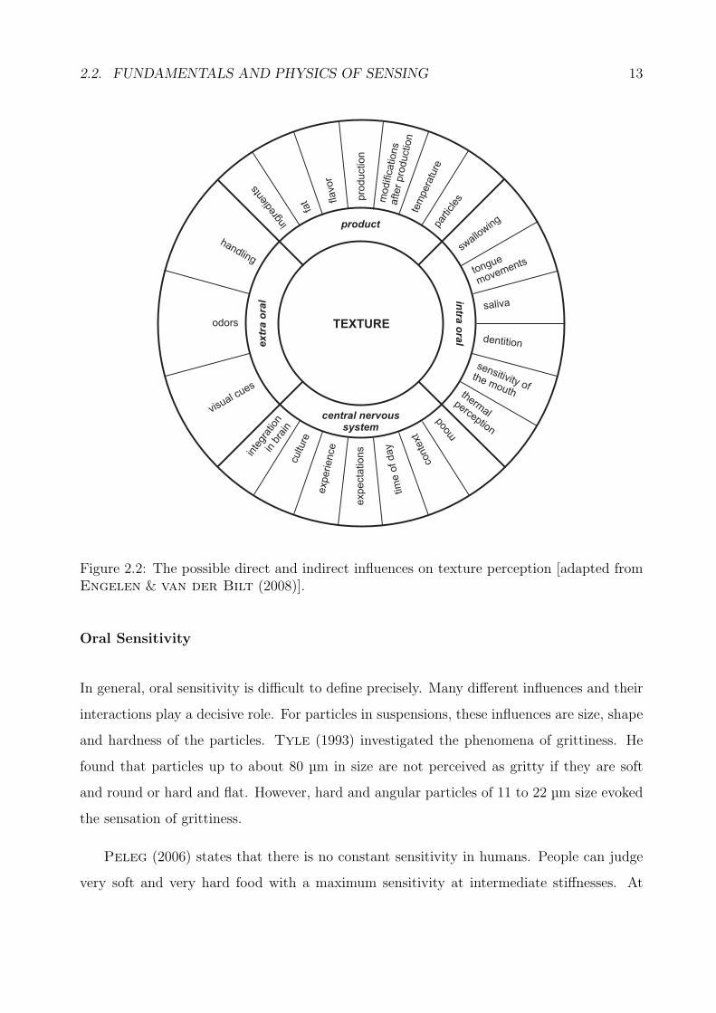
processing can hardly be mimicked by technical instruments. Figure 2.2 provides an overview
of possible direct and indirect influences on texture perception, which may be interwoven.
The physiological aspects of oral sensitivity, tongue movements, temperature and saliva
composition are especially emphasized by the authors. They conclude that oral physiology
can presumably explain some of the inter-individual variation. The current study focuses on
tongue movement and the resulting fluid flow in the oral cavity. The importance of the other
effects is beyond doubt, but neglected here due to the restrictions of the employed models.
In order to give an idea about these aspects, example studies are introduced below.
2.2. FUNDAMENTALS AND PHYSICS OF SENSING 13
flavor
product
central nervoussystem
intra
ora
lextr
a o
ral
ingr
edie
nts
fat
tem
pera
ture
partic
lesm
odific
ations
after
pro
duction
pro
duction
tongue
movements
thermal
perception
sensitivity ofthe mouth
handling
tim
eof day
moo
d
saliva
dentition
swallo
wing
experience
conte
xtvisual c
ues
odors
inte
grat
ion
inbr
ain
cultu
re
expecta
tions
TEXTURE
Figure 2.2: The possible direct and indirect influences on texture perception [adapted fromEngelen & van der Bilt (2008)].
Oral Sensitivity
In general, oral sensitivity is difficult to define precisely. Many different influences and their
interactions play a decisive role. For particles in suspensions, these influences are size, shape
and hardness of the particles. Tyle (1993) investigated the phenomena of grittiness. He
found that particles up to about 80 µm in size are not perceived as gritty if they are soft
and round or hard and flat. However, hard and angular particles of 11 to 22 µm size evoked
the sensation of grittiness.
Peleg (2006) states that there is no constant sensitivity in humans. People can judge
very soft and very hard food with a maximum sensitivity at intermediate stiffnesses. At
14 CHAPTER 2. STATE OF THE ART
both ends of the scale, however, they have difficulties to discriminate.
Strassburg, Burbidge, Delgado & Hartmann (2007) found similar results. The
authors investigated the oral evaluation of the thickness of flexible circular disks. These
disks had a constant diameter of 3 mm and a constant elastic modulus of 480 MPa. Their
thicknesses ranged from 12.5 µm to 350 µm. A range from 125 µm to 190 µm thickness
could be found in which the disk geometries could not be discerned by the tactile senses in
the mouth although the difference between two consecutively evaluated disks lies above the
known threshold of 25 µm.
Temperature
Temperature has a crucial influence on food thickness. Food has an initial temperature when
consumption starts. This temperature changes during consumption due to the thermal
diffusivity of the food and the oral temperature. This change in temperature is followed
by a viscosity change (Stanley & Taylor, 1993). The thickness of semi-solid foodstuff
decreases significantly with an increasing product temperature.
According to Rao (1977), the change of viscosity in foods due to temperature can be
calculated by
η = BeERT , (2.1)
which is known as the Arrhenius equation. Here, η stands for the viscosity, B for a
constant, E for the activation energy, R for the gas constant and T for the temperature.
The equation is valid for both Newtonian and non-Newtonian fluids. The constant B is
dependent on the weight fraction of total solids.
Engelen, de Wijk, Prinz, Janssen, Weenen & Bosman (2003) also investigated
the influence of the oral temperature on thickness perception. For that purpose, they asked
their subjects to rinse their mouths with water of different temperatures immediately before
tasting. The oral tissues slightly changed their temperature due to this procedure. The same
2.2. FUNDAMENTALS AND PHYSICS OF SENSING 15
tempered product was evaluated to have different subjective thicknesses due to the different
temperatures in the oral cavity. This effect is small, but present.
Saliva
Saliva is a viscoelastic fluid with a varying viscosity between 2 mPas and 13 mPas at high
and low shear rates (Roberts, 1977). It alters the properties of food during consumption
by warming and diluting the solution in the mouth, resulting in an inhomogeneous mixture
(Christensen & Casper, 1987). Stanley & Taylor (1993) claimed that the dilution
effect is too small to be significant, but it was observed to decrease the tendency for turbulent
flow in thin solutions (Christensen, 1984). Less turbulent flow will, in turn, lead to
decreased perceived viscosity (Parkinson & Sherman, 1971). The effects of saliva are not
taken into consideration in the current study as the duration of the process of deglutition is
short compared to the time of possible interactions of saliva with the samples.
2.2.3 Oral Food Texture Evaluation and Terminology
Christensen (1984) states that texture perception is a very complex process. Texture per-
ception requires an active manipulation and deformation of the food, which in turn modifies
the physical properties. van Aken et al. (2007) emphasized that it is necessary to apply
a little oral processing before swallowing and perceive the attributes at or shortly after food
intake for this reason.
Szczesniak (1963) defined three main classes of textural characteristics:
• mechanical characteristics - reactions according to stress,
• geometrical characteristics - arrangement of the constituents/appearance and
• other characteristics that refer mainly to moisture and fat content.
The mechanical characteristics can be classified in the five primary groups
16 CHAPTER 2. STATE OF THE ART
• hardness,
• cohesiveness,
• viscosity,
• elasticity and
• adhesiveness.
Every attribute is evaluated on a reference scale. Each rating on the specific scale is stan-
dardized with a specific product of a specific brand and manufacturer. Hence, the sensory
results are reproducible. This approach is called sensory texture profiling.
In the early 1970s, a sub-committee on Sensory Analysis of the British Standards Insti-
tution worked on food texture terminology. Jowitt, a member of this committee, proposed
the first list of food texture terminology in 1974 in order to achieve a general international
agreement. His list included
• the definition of general terms (structure, texture, consistency),
• an itemization of material behavior under applied stress or strain including definitions,
• terms describing material structure (particle size or shape, shape and arrangement of
structural elements) and
• an itemization and definitions of mouthfeel characteristics.
Additionally, Jowitt suggested a term be defined for those sensations that cannot be related
to textural properties but also influence mouthfeel, like astringency and temperature. The
general terminology includes all texture attributes for both solid and fluid food. This is
not appropriate for food capable of flowing. For this reason, special terminologies were
developed.
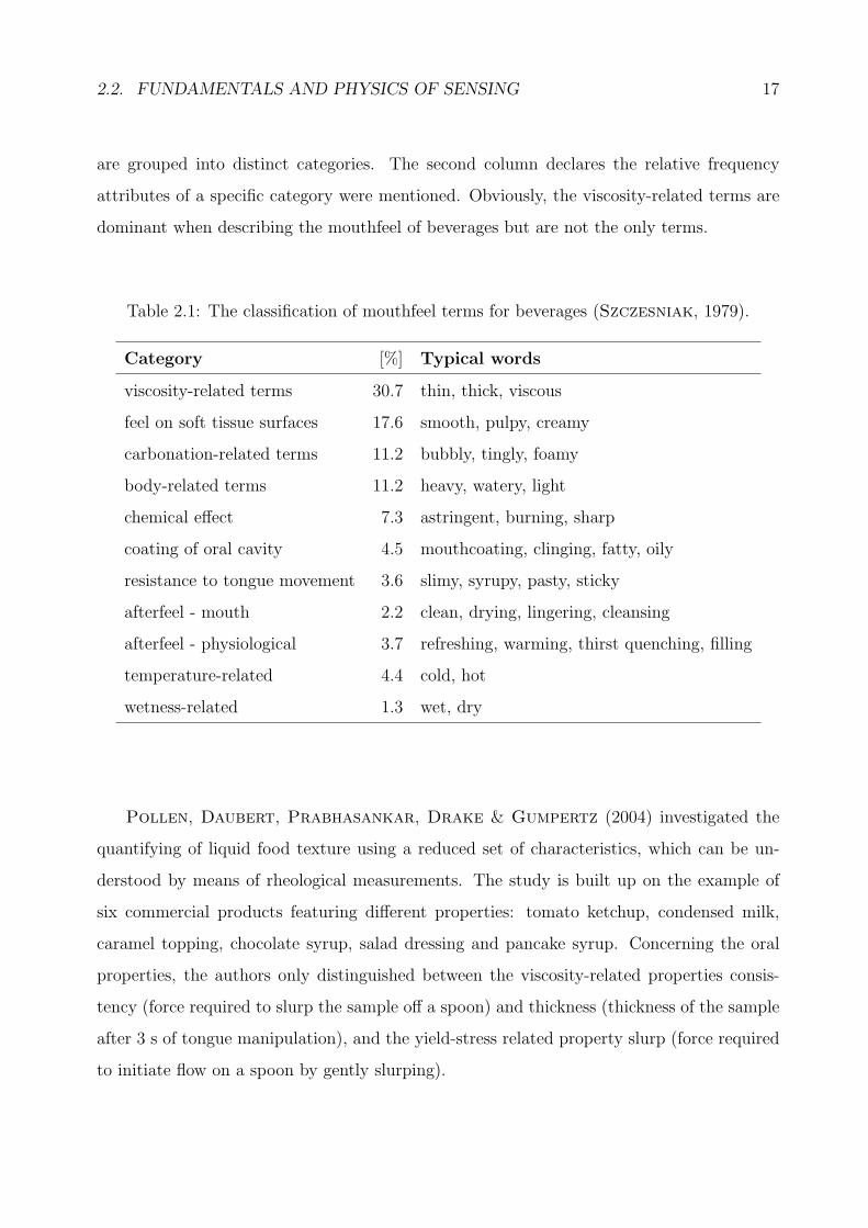
Szczesniak (1979) introduced a list of mouthfeel attributes, which arise due to the
consumption of beverages. Table 2.1 gives an overview of the occurring attributes, which
2.2. FUNDAMENTALS AND PHYSICS OF SENSING 17
are grouped into distinct categories. The second column declares the relative frequency
attributes of a specific category were mentioned. Obviously, the viscosity-related terms are
dominant when describing the mouthfeel of beverages but are not the only terms.
Table 2.1: The classification of mouthfeel terms for beverages (Szczesniak, 1979).
Category [%] Typical words
viscosity-related terms 30.7 thin, thick, viscous
feel on soft tissue surfaces 17.6 smooth, pulpy, creamy
carbonation-related terms 11.2 bubbly, tingly, foamy
body-related terms 11.2 heavy, watery, light
chemical effect 7.3 astringent, burning, sharp
coating of oral cavity 4.5 mouthcoating, clinging, fatty, oily
resistance to tongue movement 3.6 slimy, syrupy, pasty, sticky
afterfeel - mouth 2.2 clean, drying, lingering, cleansing
afterfeel - physiological 3.7 refreshing, warming, thirst quenching, filling
temperature-related 4.4 cold, hot
wetness-related 1.3 wet, dry
Pollen, Daubert, Prabhasankar, Drake & Gumpertz (2004) investigated the
quantifying of liquid food texture using a reduced set of characteristics, which can be un-
derstood by means of rheological measurements. The study is built up on the example of
six commercial products featuring different properties: tomato ketchup, condensed milk,
caramel topping, chocolate syrup, salad dressing and pancake syrup. Concerning the oral
properties, the authors only distinguished between the viscosity-related properties consis-
tency (force required to slurp the sample off a spoon) and thickness (thickness of the sample
after 3 s of tongue manipulation), and the yield-stress related property slurp (force required
to initiate flow on a spoon by gently slurping).
18 CHAPTER 2. STATE OF THE ART
2.2.4 Oral Shear Stresses and Shear Rates
Janssen, Terpstra, de Wijk & Prinz (2007) state that the exact range of shear rates
in the mouth is not known, although several attempts employing different strategies have
been undertaken in order to find a remedy. Some scientists came from an experimental
background, others from a mathematical one. These approaches are presented separately in
the following sections.
Experimental Approaches
First approaches, for example the approach from Stevens & Guirao (1964), established
empirical relationships in terms of a power function between subjective and objective at-
tributes of viscosity emanating from perception and rheology. A pioneer in this field of
research was Wood (1968) who characterized different foodstuffs and a Newtonian solution
rheologically. Equivalent shear stresses and shear rates occur at the intersection points of
the Newtonian curve with the non-Newtonian curves in a diagram of shear stress vs shear
rate.
Panelists were asked to evaluate the viscosities of the non-Newtonian foods compared to
the Newtonian solution. The non-Newtonian foods that came closest in perceived consistency
defined the shear-rate range employed for the oral evaluation. Wood concluded that the
shear rate that is relevant for the perception of thickness is about 50 s−1. He hypothesized
that the corresponding shear stress is the perceived stimulus.
Years later, Cook, Hollowood, Linforth & Taylor (2003) confirmed this hypothe-
sis by stating that shear stress is the stimulus that is used for the oral evaluation of viscosity.
Thus, it has a special meaning for the somatosensory sense (see chapter 2.3). Apart from the
detection of flow by means of the mechanoreceptors located in the surfaces of the oral tissues,
the solution’s resistance to flow is detected by the intramuscular receptors of the kinesthetic
sense (Christensen & Casper, 1987). They measure the force or effort applied to move
the solution.
2.2. FUNDAMENTALS AND PHYSICS OF SENSING 19
Employing the same strategy as Wood, Shama & Sherman (1973) investigated oral
shear rates and shear stresses over a wider range of food viscosities. Similar foods were
grouped together with a Newtonian solution of a comparable viscosity. The area where
rheological and sensory measurements agreed was marked by a broken line rectangle in their
graph of shear stress vs shear rate.
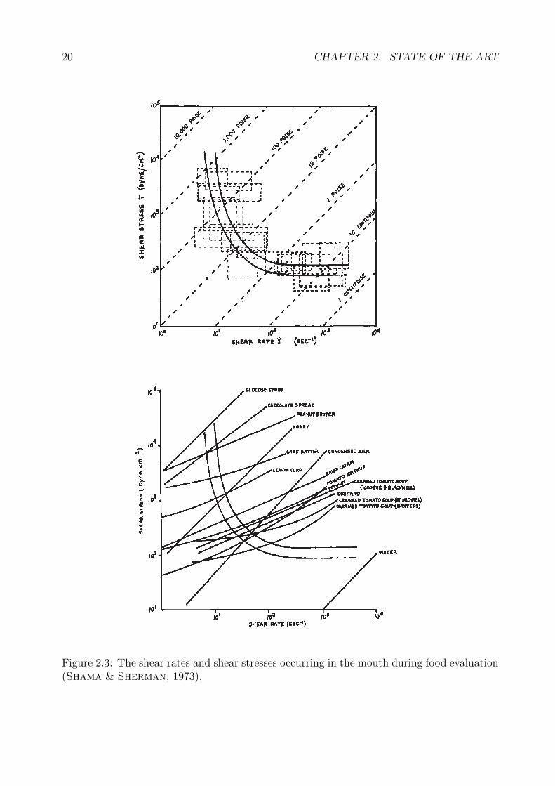
The upper diagram in figure 2.3 shows the resulting rectangles. The two continuous
curves represent the approximate limits of shear rates and shear stresses in which foods were
evaluated in the oral cavity. It was concluded that oral shear rates lie between 10 s−1 and
1000 s−1, and the resulting oral shear stresses between 10 Pa and 1000 Pa. Furthermore, the
results suggest that stimuli of liquid foods can be traced back to shear rates evaluated at
approximately constant shear stresses of about 10 Pa. In viscous foods, shear stresses at an
approximately constant shear rate of 10 s−1 are responsible for the stimuli.
The lower diagram in figure 2.3 delivers information about the evaluated foods. Their
rheological characteristics are superimposed upon the continuous curves in the upper dia-
gram. Hence, it is possible to estimate the shear rate and shear stress that occur in the oral
cavity for each single foodstuff.
The correlation between shear rates and stresses, and foodstuffs is quite good. Neverthe-
less, Christensen (1979) makes the alternative assumption that a certain range of shear
rates is always generated in the oral cavity. Panelists evaluate the viscosity of the solution
along the whole shear rate range and come up with an averaged viscosity. This would explain
why solutions of carboxymethylcellulose of different polymer length but identical viscosity
are evaluated to be thinner the more distinct their non-Newtonian behavior is. Cutler,
Morris & Taylor (1983) came to a similar conclusion, but added that objective viscosity
measurements at 10 s−1 correlate well with the perceived thickness of most fluids.
Houska, Valentova, Novotna, Strohalm, Sestak & Pokorny (1998) employed
five different sensory methods (mixing with a spoon, pouring from a spoon, slurping from
a spoon, compressing between tongue and palate, and swallowing effort) in order to evalu-
ate rheologically-measured samples. The authors established power-law functions between
20 CHAPTER 2. STATE OF THE ART
Figure 2.3: The shear rates and shear stresses occurring in the mouth during food evaluation(Shama & Sherman, 1973).
2.2. FUNDAMENTALS AND PHYSICS OF SENSING 21
the sensory evaluations and the rheological measurements. They found shear rates up to
questionable 15307470 s−1 for the slurping of low viscosity strawberry-yogurt drinks.
Other approaches have employed dynamic-viscosity measurements combined with smaller
deformations than the steady-shear approaches used before (Stanley & Taylor, 1993).
Bistany & Kokini (1983) were the first who showed that the dynamic viscosities are much
larger than the steady viscosities. Richardson, Morris, Ross-Murphy, Taylor &
Dea (1989) found that the measurements under oscillatory shear at the single frequency of
50 rad/s correlate directly with panel scores for the perceived thickness of solutions with and
without yield stress.
Analytical Approaches
Starting in the 1970s, the groups of the researchers Cussler and Kokini developed a math-
ematical model for the prediction of subjective attributes. In a first attempt, DeMartine
& Cussler (1975) developed a set of equations in order to predict the subjective spreadabil-
ity, viscosity and stickiness evaluated by using one’s fingers. The mathematical model was
developed in three steps. At first, the fingers were approximated by two parallel plates and
the fluid rheology by the power law. Then the film thickness of the fluid was expressed by
means of the Stefan equation, which can be derived from the theory of lubrication. This
theory is introduced in detail in chapter 3.3. DeMartine & Cussler implemented the
power law in the friction term of an equation of squeezing flow and solved the equation for
the fluid film. The height of the film is dependent on time, plate radius and fluid rheology.
The final step, the prediction, was based on the developed equation. The authors assume
proportionalities between spreadability and reciprocal shear rate, viscosity and shear rate,
and stickiness and the quotient of the initial height and plate velocity.
The subjects evaluated the samples by using their fingers. Spreadability was evaluated
by spreading the sample along a plate with the index finger, viscosity by rubbing the fluid
between the fingers and stickiness by removing the finger after touching the fluid on the
22 CHAPTER 2. STATE OF THE ART
plate. These measurements were compared to the results of the equations. The successful
fits exhibit correlation coefficients of at least 0.90.
Kokini, Kadane & Cussler (1977) applied the preceding ideas to the tongue-palate
system in the mouth. Again, they approximated the tongue and palate by a system of two
parallel plates. Ten original attributes were reduced to three, which were related to physical
quantities. Thickness was related with viscous forces, smoothness with frictional forces, and
slipperiness with a combination of both. The rest of the procedure remains the same as
described above.
On the basis of this mathematical model, Dickie & Kokini (1983) calculated the shear
rates that are supposed to occur in the mouth. They came out with a range between 5.09 s−1
for thicker foods like marshmallows and 36.50 s−1 for thinner foods such as ketchup assuming
the fluids follow the power law.
Elejalde & Kokini (1992) stated that shear stress in the mouth is the sensory mech-
anism used for the oral evaluation of viscosity. For this reason, they used the model intro-
duced above in order to calculate shear rates and shear stresses. They performed their own
study using syrups. Their rheological characterizations yielded shear rates in the range from
11.78 s−1 to 99.78 s−1 and shear stresses in the range from 4.4 Pa to 131 Pa. In order to
verify the model, they employed further data published by Cutler et al. (1983). These
data led to a minimum shear rate of 10.03 s−1 for lemon curd and a maximum shear rate of
415.99 s−1 for fresh milk. The calculated shear stresses ranged between 1.0 Pa for fresh milk
and 683 Pa for chocolate spread.
Other authors enhanced the findings introduced above. Campanella & Peleg (1987)
deduced an advanced mathematical model consisting of one rigid and one elastic plate. The
elastic plate represents the deformable tissue of the tongue. The authors quantified the effect
on the force-time curve dimensionlessly. Nicosia & Robbins (2001) used the rigid set-up
in order to investigate the fluid mechanics of bolus ejection from the oral cavity, with close
attention regarding the bolus-ejection time.
2.2. FUNDAMENTALS AND PHYSICS OF SENSING 23
2.2.5 Numerical Simulations
Numerical simulations in structural and fluid mechanics are a powerful and efficient tool to
calculate shear and normal stresses in solid and liquid materials. The method is employed
when analytical solutions fail due to the complexity of the geometry. The application of
numerical simulations provides the required insight into those complex systems (Datta,
1998).
The area of application is widespread in all disciplines of engineering, ranging from auto-
motive engineering to medical technology. This section gives a concise overview of numerical
simulations relating to different aspects of oral biomechanics. The motivation of previous
investigations was dominated by medical questions like implant dentistry, rehabilitation after
tongue surgeries and dysphagia. Additionally, there is a bionics-motivated study about ram
feeding fish.
Nowadays, finite element analysis is a very common method in implant dentistry. Wein-
stein, Klawitter, Anand & Schuessler (1976) published the first paper in this area of
research. They performed a two-dimensional stress analysis in porous rooted dental implants,
after which the method gained ground.
At the beginning of the last decade, Geng, Tan & Liu (2001) composed a review paper
about the advances in biomechanics of dental implants. Emphasis was put on the prediction
of stress on implants and their surrounding bones due to mastication. In this context, the
three aspects of bone-implant interface, implant-prosthesis connection and multiple-implant
prosthesis are of importance.
Only recently, Wakabayashi, Ona, Suzuki & Igarashi (2008) published another re-
view article about nonlinear finite element analyses for dental applications. The authors state
that nonlinear stress-strain relationships mirror the intraoral environment more realistically.
The aspects of displacement of periodontal ligament, plastic and viscoelastic behaviors in
restoration materials, tooth-to-tooth contact, mechanical contacts of implant prostheses and
tooth-restoration complexes were discussed in detail.
24 CHAPTER 2. STATE OF THE ART
Tongue movement is another branch analyzed by means of structural-mechanics ap-
proaches. The deformable nature of the tongue turns out to be a great challenge to simulate.
Nevertheless, modern computer hardware enables the highly complicated realization of this
ambitious objective.
Vogt, Lloyd, Buchaillard, Perrier, Chabanas, Payan & Fels (2006) devel-
oped an innovative three-dimensional biomedical finite-element-based simulation of a muscle-
activated human tongue with a simulation time ten times larger than real-time. Their inten-
tion was to contribute to the clarification of physiological activities like speech production,
breathing and swallowing, surgical and dental training, and outcome prediction for clinical
procedures.
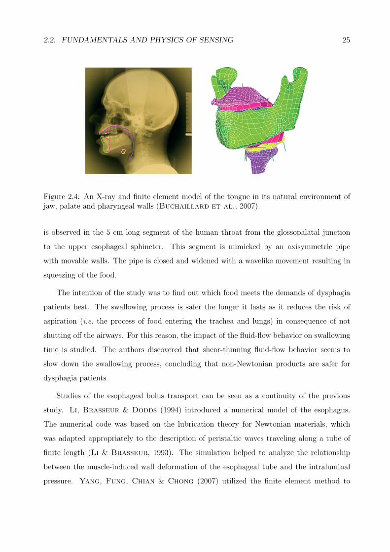
In a next step, Buchaillard, Brix, Perrier & Payan (2007) extended the model
including jaw, palate and pharyngeal walls, as can be seen in figure 2.4. By means of this
model, the effect of tissue loss and reconstruction on the tongue movement was studied.
In particular, the study deals with two common tongue surgeries used to remove tongue
tumors, namely hemiglossectomy, which is the surgical removal of one half of the tongue,
and mouth-floor resection. Subsequent reconstruction is modeled implementing flaps of
different stiffness. These simulations clarify the potential impact on speech articulation.
The long-term perspective is to adapt the simulation individually. The method can thereby
contribute to help cancer patients in regaining quality of life.
Oral fluid mechanics has been analyzed only rarely using numerical simulations. Excep-
tions are some studies of oropharyngeal mechanics for a greater understanding of dysphagia.
Chang, Rosendall & Finlayson (1998) and Meng, Rao & Datta (2005) simulate the
pharyngeal bolus transport of isothermal, homogeneous and incompressible Newtonian and
non-Newtonian fluids. The Newtonian fluid flow was represented using the dynamic viscos-
ity η = 1 mPas and the density ρ = 1000 kg/m3 as well as the parameters η = 150 mPas
and ρ = 1800 kg/m3. Non-Newtonian behavior was reflected by the power law σ = Kγn.
The consistency index was set to K = 2.0Pasn, the flow behavior index n = 0.7. As the
exponent n is < 1, the fluid-flow behavior is shear-thinning. The pharyngeal bolus transport
2.2. FUNDAMENTALS AND PHYSICS OF SENSING 25
Figure 2.4: An X-ray and finite element model of the tongue in its natural environment ofjaw, palate and pharyngeal walls (Buchaillard et al., 2007).
is observed in the 5 cm long segment of the human throat from the glossopalatal junction
to the upper esophageal sphincter. This segment is mimicked by an axisymmetric pipe
with movable walls. The pipe is closed and widened with a wavelike movement resulting in
squeezing of the food.
The intention of the study was to find out which food meets the demands of dysphagia
patients best. The swallowing process is safer the longer it lasts as it reduces the risk of
aspiration (i.e. the process of food entering the trachea and lungs) in consequence of not
shutting off the airways. For this reason, the impact of the fluid-flow behavior on swallowing
time is studied. The authors discovered that shear-thinning fluid-flow behavior seems to
slow down the swallowing process, concluding that non-Newtonian products are safer for
dysphagia patients.
Studies of the esophageal bolus transport can be seen as a continuity of the previous
study. Li, Brasseur & Dodds (1994) introduced a numerical model of the esophagus.
The numerical code was based on the lubrication theory for Newtonian materials, which
was adapted appropriately to the description of peristaltic waves traveling along a tube of
finite length (Li & Brasseur, 1993). The simulation helped to analyze the relationship
between the muscle-induced wall deformation of the esophageal tube and the intraluminal
pressure. Yang, Fung, Chian & Chong (2007) utilized the finite element method to
26 CHAPTER 2. STATE OF THE ART
illustrate the interaction of tissue, Newtonian food bolus and the peristaltic wave due to
muscle contraction for the first time.
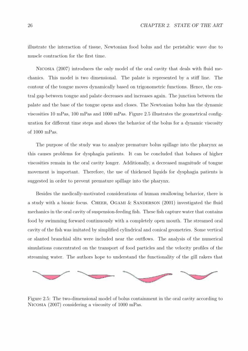
Nicosia (2007) introduces the only model of the oral cavity that deals with fluid me-
chanics. This model is two dimensional. The palate is represented by a stiff line. The
contour of the tongue moves dynamically based on trigonometric functions. Hence, the cen-
tral gap between tongue and palate decreases and increases again. The junction between the
palate and the base of the tongue opens and closes. The Newtonian bolus has the dynamic
viscosities 10 mPas, 100 mPas and 1000 mPas. Figure 2.5 illustrates the geometrical config-
uration for different time steps and shows the behavior of the bolus for a dynamic viscosity
of 1000 mPas.
The purpose of the study was to analyze premature bolus spillage into the pharynx as
this causes problems for dysphagia patients. It can be concluded that boluses of higher
viscosities remain in the oral cavity longer. Additionally, a decreased magnitude of tongue
movement is important. Therefore, the use of thickened liquids for dysphagia patients is
suggested in order to prevent premature spillage into the pharynx.
Besides the medically-motivated considerations of human swallowing behavior, there is
a study with a bionic focus. Cheer, Ogami & Sanderson (2001) investigated the fluid
mechanics in the oral cavity of suspension-feeding fish. These fish capture water that contains
food by swimming forward continuously with a completely open mouth. The streamed oral
cavity of the fish was imitated by simplified cylindrical and conical geometries. Some vertical
or slanted branchial slits were included near the outflows. The analysis of the numerical
simulations concentrated on the transport of food particles and the velocity profiles of the
streaming water. The authors hope to understand the functionality of the gill rakers that
Figure 2.5: The two-dimensional model of bolus containment in the oral cavity according toNicosia (2007) considering a viscosity of 1000 mPas.
2.3. PHYSIOLOGY OF TEXTURE PERCEPTION 27
retain food organisms at the gill arch filaments. The ultimate aim of their work is to design
industrial hydrosol filtration methods modeled on these effective ram suspension feeders.
2.3 Physiology of Texture Perception
Food texture is perceived by both tactile and kinesthetic senses (Kilcast & Eves, 1991,
Christensen, 1984, Verhagen & Engelen, 2006). The tactile sense perceives touch on
the surface of the skin. Therefore, this sense transmits stimuli from the environment. The
surfaces of the oral cavity that receive this kind of stimuli by means of mechanoreceptors
are the tongue, the palate and the pharyngeal regions.
In contrast, the kinesthetic sense is an internal body sense. It delivers information
concerning the static position of specific parts of the body and the relative position of several
parts to each other. Additionally, it measures the effort required for motion. In the case of
the oral cavity this sense is important for the movement of the jaw and tongue. Occurring
stimuli are transmitted by proprioceptors. The most relevant receptors in kinesthesis are
muscle spindles. They send signals due to changes in their length.
The stimulation of a receptor is followed by a signal transduction pathway via nerve
cells, the so-called axons. Mechanoreceptors are stimulated by deformations of their cell
membrane. These deformations result in an opening of ion channels. In consequence of the
ion exchange the cells are depolarized. If a certain threshold of depolarization is achieved an
action potential will be sent. This is a temporary change of voltage, which is transmitted from
axon to axon to the brain. Long-lasting depolarizations trigger series of action potentials.
The frequency of the action potentials decreases with time until the resting potential of
the cell is recovered. Hence, a constant stimulation leads to an adaptation of the receptor.
Finally, the signal patterns that are sent are decoded and analyzed in the brain (Morike,
Betz & Mergenthaler, 1997, Schmidt, 1998).
28 CHAPTER 2. STATE OF THE ART
2.3.1 Classification of the Mechanoreceptors
As the tactile sense is supposed to be the most relevant one for texture perception, it is
presented here. In general, there are four different types of mechanoreceptors. Each of them
has different perceptual functions. The single transmitted stimuli responses correspond to a
specific tactile sensation (Johnson, 2001).
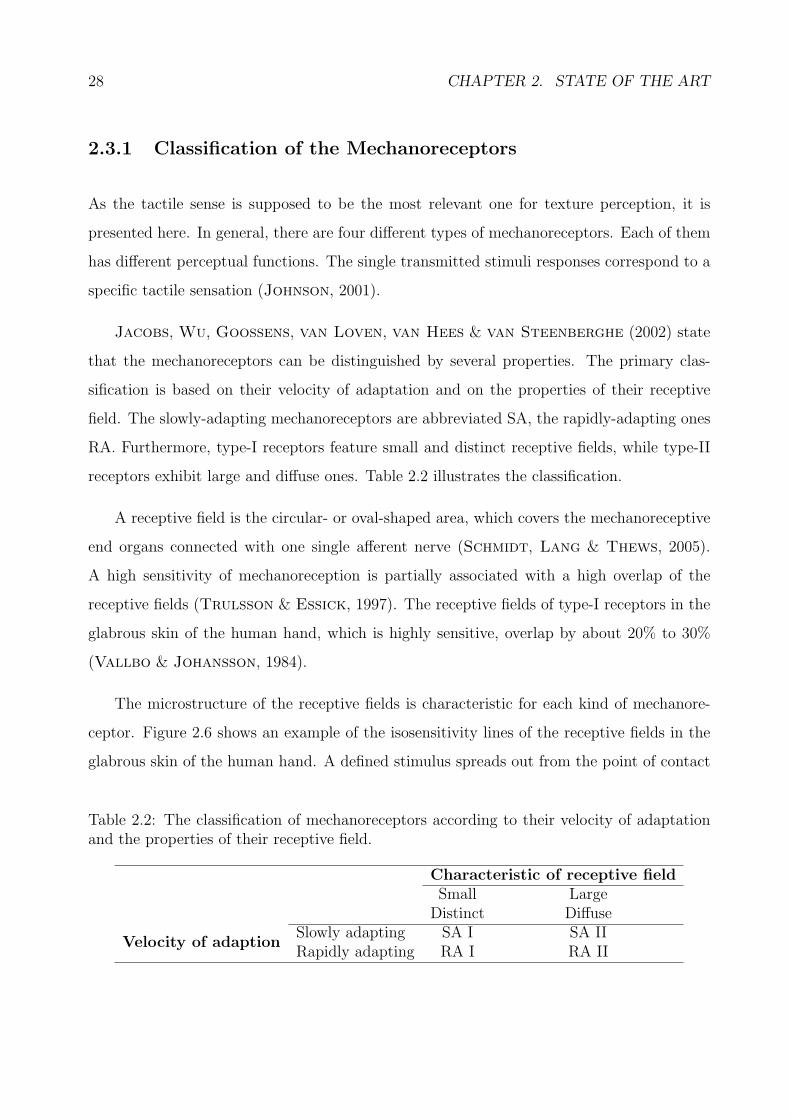
Jacobs, Wu, Goossens, van Loven, van Hees & van Steenberghe (2002) state
that the mechanoreceptors can be distinguished by several properties. The primary clas-
sification is based on their velocity of adaptation and on the properties of their receptive
field. The slowly-adapting mechanoreceptors are abbreviated SA, the rapidly-adapting ones
RA. Furthermore, type-I receptors feature small and distinct receptive fields, while type-II
receptors exhibit large and diffuse ones. Table 2.2 illustrates the classification.
A receptive field is the circular- or oval-shaped area, which covers the mechanoreceptive
end organs connected with one single afferent nerve (Schmidt, Lang & Thews, 2005).
A high sensitivity of mechanoreception is partially associated with a high overlap of the
receptive fields (Trulsson & Essick, 1997). The receptive fields of type-I receptors in the
glabrous skin of the human hand, which is highly sensitive, overlap by about 20% to 30%
(Vallbo & Johansson, 1984).
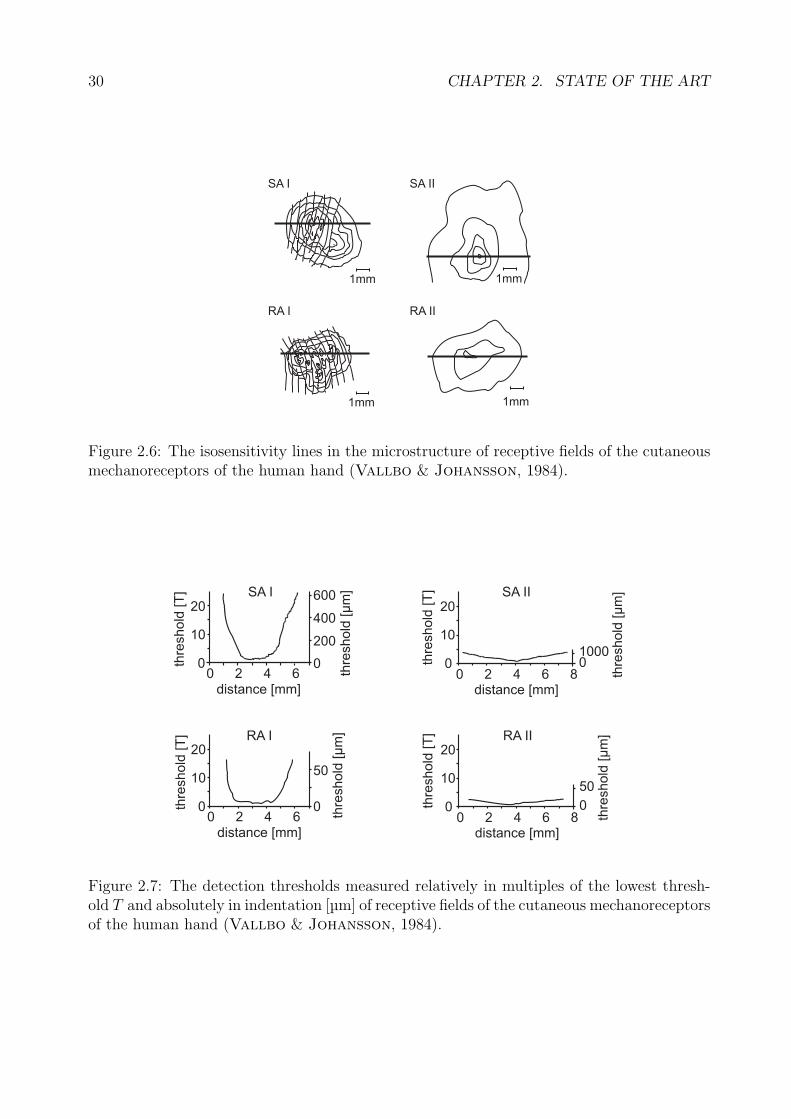
The microstructure of the receptive fields is characteristic for each kind of mechanore-
ceptor. Figure 2.6 shows an example of the isosensitivity lines of the receptive fields in the
glabrous skin of the human hand. A defined stimulus spreads out from the point of contact
Table 2.2: The classification of mechanoreceptors according to their velocity of adaptationand the properties of their receptive field.
Characteristic of receptive fieldSmall Large
Distinct Diffuse
Velocity of adaptionSlowly adapting SA I SA IIRapidly adapting RA I RA II
2.3. PHYSIOLOGY OF TEXTURE PERCEPTION 29
to a line representing a certain sensitivity. Hence, the size of the receptive field increases
with the power of the stimulus.
The type-I receptors exhibit a dense occurrence of isosensitivity lines including four
to seven sensitivity peaks in case of SA receptors and 12 to 17 in case of RA receptors.
These sensitivity peaks can presumably be ascribed to the exact number of end organs or
the number of end-organ clusters connected to one parent axon. In contrast, the type-II
receptors exhibit sparse isosensitivity lines and only one single sensitivity peak.
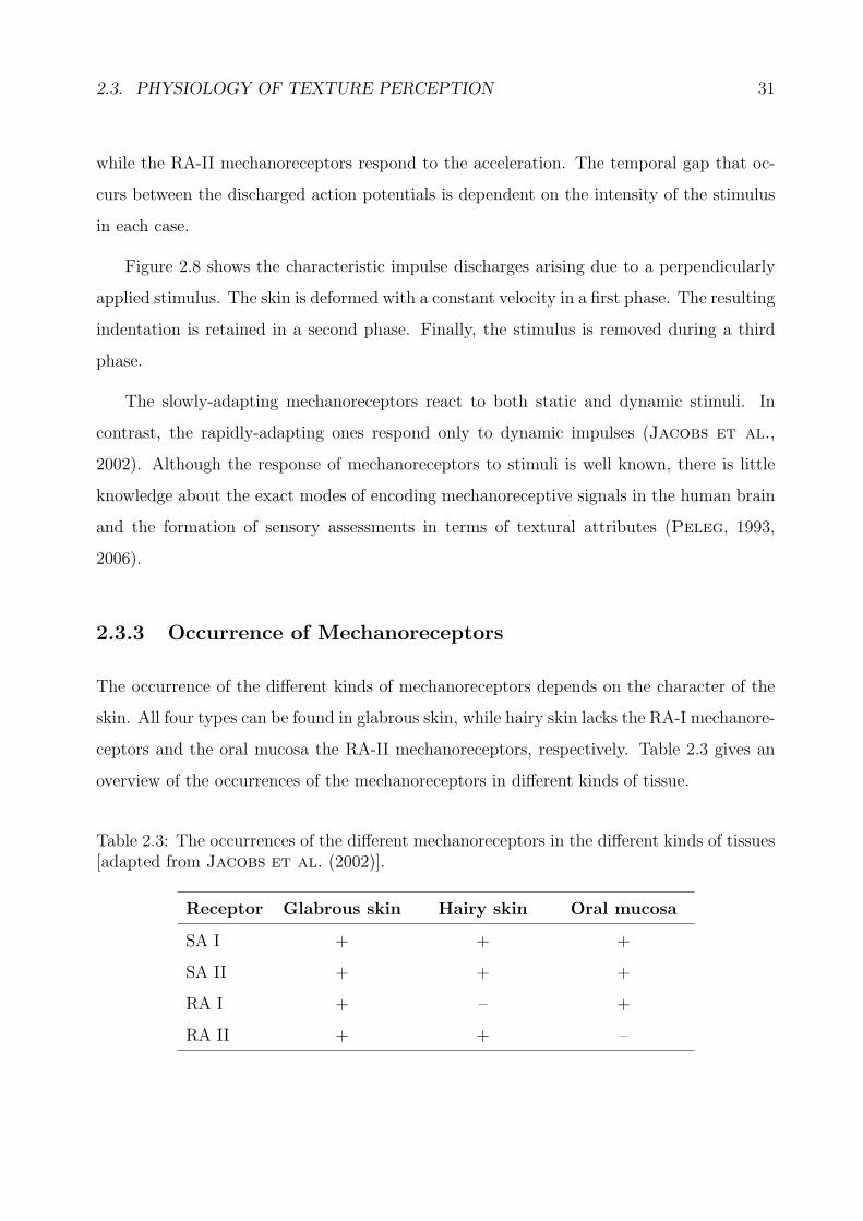
Figure 2.7 depicts the detection thresholds along the lines plotted in figure 2.6. The
figure represents the smallest detectable level of mechanoreception possible. The abscissa
represents the distance in mm. The left ordinate displays the detection threshold as a
multiple of the lowest threshold T , the right ordinate the absolute indentation threshold in
µm.
The threshold is very low over a wide range in the case of the type-I receptors. It increases
to a twentyfold value at the borders of the receptive field. Therewith, the receptive fields
of type-I receptors are distinct. These borders are missing in the case of type-II receptors.
Here, the sensitivity falls off gently over the complete distance. Furthermore, the threshold
only achieves fivefold values comparing the center and border of the receptive field.
The absolute indentation thresholds differ strongly. While the maximum occurring
threshold is 50 µm for RA receptors, SA receptors have a threshold of 600 µm and 1000 µm,
respectively.
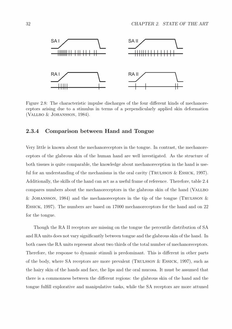
2.3.2 Impulse-Discharge Patterns
The different types of mechanoreceptors respond to different modes of skin deformation
(Schmidt et al., 2005). The SA-I mechanoreceptors react to the intensity of skin im-
pression, which is a stress causing deformation from the mechanical point of view. The
SA-II mechanoreceptors are sensitive to the intensity of skin stretch, which is equivalent
with strain. The RA-I mechanoreceptors respond to the velocity of the skin deformation,
30 CHAPTER 2. STATE OF THE ART
1mm
1mm
1mm
1mm
SA I SA II
RA I RA II
Figure 2.6: The isosensitivity lines in the microstructure of receptive fields of the cutaneousmechanoreceptors of the human hand (Vallbo & Johansson, 1984).
20
10
0thre
sh
old
[T
]
0 2 4 6
distance [mm]
0
50
thre
sh
old
[µ
m]RA I
0 2 4 6
distance [mm]
600
400
0
200
20
10
0thre
sh
old
[T
]
thre
sh
old
[µ
m]SA I
20
10
0thre
sh
old
[T
]
0 2 4 6distance [mm]
801000
thre
sh
old
[µ
m]SA II
20
10
0thre
sh
old
[T
]
0 2 4 6distance [mm]
80
50
thre
sh
old
[µ
m]RA II
Figure 2.7: The detection thresholds measured relatively in multiples of the lowest thresh-old T and absolutely in indentation [µm] of receptive fields of the cutaneous mechanoreceptorsof the human hand (Vallbo & Johansson, 1984).
2.3. PHYSIOLOGY OF TEXTURE PERCEPTION 31
while the RA-II mechanoreceptors respond to the acceleration. The temporal gap that oc-
curs between the discharged action potentials is dependent on the intensity of the stimulus
in each case.
Figure 2.8 shows the characteristic impulse discharges arising due to a perpendicularly
applied stimulus. The skin is deformed with a constant velocity in a first phase. The resulting
indentation is retained in a second phase. Finally, the stimulus is removed during a third
phase.
The slowly-adapting mechanoreceptors react to both static and dynamic stimuli. In
contrast, the rapidly-adapting ones respond only to dynamic impulses (Jacobs et al.,
2002). Although the response of mechanoreceptors to stimuli is well known, there is little
knowledge about the exact modes of encoding mechanoreceptive signals in the human brain
and the formation of sensory assessments in terms of textural attributes (Peleg, 1993,
2006).
2.3.3 Occurrence of Mechanoreceptors
The occurrence of the different kinds of mechanoreceptors depends on the character of the
skin. All four types can be found in glabrous skin, while hairy skin lacks the RA-I mechanore-
ceptors and the oral mucosa the RA-II mechanoreceptors, respectively. Table 2.3 gives an
overview of the occurrences of the mechanoreceptors in different kinds of tissue.
Table 2.3: The occurrences of the different mechanoreceptors in the different kinds of tissues[adapted from Jacobs et al. (2002)].
Receptor Glabrous skin Hairy skin Oral mucosa
SA I + + +
SA II + + +
RA I + – +
RA II + + –
32 CHAPTER 2. STATE OF THE ART
SA I SA II
RA I RA II
Figure 2.8: The characteristic impulse discharges of the four different kinds of mechanore-ceptors arising due to a stimulus in terms of a perpendicularly applied skin deformation(Vallbo & Johansson, 1984).
2.3.4 Comparison between Hand and Tongue
Very little is known about the mechanoreceptors in the tongue. In contrast, the mechanore-
ceptors of the glabrous skin of the human hand are well investigated. As the structure of
both tissues is quite comparable, the knowledge about mechanoreception in the hand is use-
ful for an understanding of the mechanisms in the oral cavity (Trulsson & Essick, 1997).
Additionally, the skills of the hand can act as a useful frame of reference. Therefore, table 2.4
compares numbers about the mechanoreceptors in the glabrous skin of the hand (Vallbo
& Johansson, 1984) and the mechanoreceptors in the tip of the tongue (Trulsson &
Essick, 1997). The numbers are based on 17000 mechanoreceptors for the hand and on 22
for the tongue.
Though the RA II receptors are missing on the tongue the percentile distribution of SA
and RA units does not vary significantly between tongue and the glabrous skin of the hand. In
both cases the RA units represent about two thirds of the total number of mechanoreceptors.
Therefore, the response to dynamic stimuli is predominant. This is different in other parts
of the body, where SA receptors are more prevalent (Trulsson & Essick, 1997), such as
the hairy skin of the hands and face, the lips and the oral mucosa. It must be assumed that
there is a commonness between the different regions: the glabrous skin of the hand and the
tongue fulfill explorative and manipulative tasks, while the SA receptors are more attuned

2.3. PHYSIOLOGY OF TEXTURE PERCEPTION 33
Table 2.4: The values of the mechanoreceptors in the glabrous skin of the human hand (H)(Vallbo & Johansson, 1984) and the mechanoreceptors in the tip of the tongue (T)(Trulsson & Essick, 1997).
SA I SA II RA I RA II
H T H T H T H T
Occurrence [%] 25 9 19 27 43 64 13 –
Median size of receptive field[mm2] 11.0 1.0 59 5.3 12.6 2.0 101 –
Diameter assuming circular re-ceptive fields [mm] 3.7 0.36 8.7 2.6 4.0 0.5 11.3 –
Innervation density per cm2 70 – 10 – 140 – 20 –
Detection threshold [mN] – 0.19 – 0.31 – 0.11 – –
to proprioception.
The median size of the receptive fields is generally smaller at the tip of the tongue than
at the hand. This confirms that the tactile acuity of the tongue is by far bigger than in
any other part of the body. The innervation density, along with the overlap of the receptive
fields, is an index for the sensitivity of mechanoreception (Trulsson & Essick, 1997).
These densities are not known for the tip of the tongue. Due to the comparability of hand
and tongue, the innervation densities of the hand act as an indication for the tongue. The
innervation density of the RA units is twice as high as that of the SA units. Analogous to
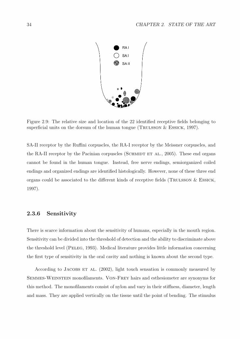
their occurrence, the RA mechanoreceptors play the predominant role. Figure 2.9 presents
the relative size and distribution of the 22 mechanoreceptive units identified on the tip of
the tongue.
2.3.5 Histological Classification of the End Organs
The end organs of the different kinds of mechanoreceptors are identified histologically in
glabrous and hairy skin. Here, the SA-I receptor is represented by the Merkel cells, the
34 CHAPTER 2. STATE OF THE ART
Figure 2.9: The relative size and location of the 22 identified receptive fields belonging tosuperficial units on the dorsum of the human tongue (Trulsson & Essick, 1997).
SA-II receptor by the Ruffini corpuscles, the RA-I receptor by the Meissner corpuscles, and
the RA-II receptor by the Pacinian corpuscles (Schmidt et al., 2005). These end organs
cannot be found in the human tongue. Instead, free nerve endings, semiorganized coiled
endings and organized endings are identified histologically. However, none of these three end
organs could be associated to the different kinds of receptive fields (Trulsson & Essick,
1997).
2.3.6 Sensitivity
There is scarce information about the sensitivity of humans, especially in the mouth region.
Sensitivity can be divided into the threshold of detection and the ability to discriminate above
the threshold level (Peleg, 1993). Medical literature provides little information concerning
the first type of sensitivity in the oral cavity and nothing is known about the second type.
According to Jacobs et al. (2002), light touch sensation is commonly measured by
Semmes-Weinstein monofilaments. Von-Frey hairs and esthesiometer are synonyms for
this method. The monofilaments consist of nylon and vary in their stiffness, diameter, length
and mass. They are applied vertically on the tissue until the point of bending. The stimulus
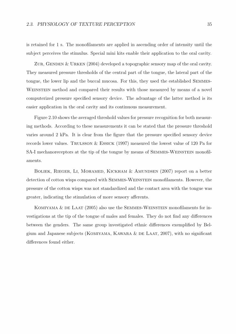
2.3. PHYSIOLOGY OF TEXTURE PERCEPTION 35
is retained for 1 s. The monofilaments are applied in ascending order of intensity until the
subject perceives the stimulus. Special mini kits enable their application to the oral cavity.
Zur, Genden & Urken (2004) developed a topographic sensory map of the oral cavity.
They measured pressure thresholds of the central part of the tongue, the lateral part of the
tongue, the lower lip and the buccal mucosa. For this, they used the established Semmes-
Weinstein method and compared their results with those measured by means of a novel
computerized pressure specified sensory device. The advantage of the latter method is its
easier application in the oral cavity and its continuous measurement.
Figure 2.10 shows the averaged threshold values for pressure recognition for both measur-
ing methods. According to these measurements it can be stated that the pressure threshold
varies around 2 kPa. It is clear from the figure that the pressure specified sensory device
records lower values. Trulsson & Essick (1997) measured the lowest value of 120 Pa for
SA-I mechanoreceptors at the tip of the tongue by means of Semmes-Weinstein monofil-
aments.
Boliek, Rieger, Li, Mohamed, Kickham & Amundsen (2007) report on a better
detection of cotton wisps compared with Semmes-Weinstein monofilaments. However, the
pressure of the cotton wisps was not standardized and the contact area with the tongue was
greater, indicating the stimulation of more sensory afferents.
Komiyama & de Laat (2005) also use the Semmes-Weinstein monofilaments for in-
vestigations at the tip of the tongue of males and females. They do not find any differences
between the genders. The same group investigated ethnic differences exemplified by Bel-
gium and Japanese subjects (Komiyama, Kawara & de Laat, 2007), with no significant
differences found either.
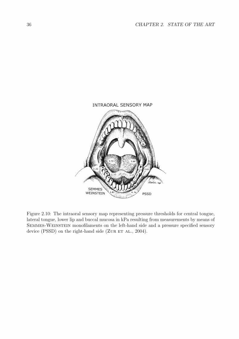
36 CHAPTER 2. STATE OF THE ART
Figure 2.10: The intraoral sensory map representing pressure thresholds for central tongue,lateral tongue, lower lip and buccal mucosa in kPa resulting from measurements by means ofSemmes-Weinstein monofilaments on the left-hand side and a pressure specified sensorydevice (PSSD) on the right-hand side (Zur et al., 2004).
Chapter 3
Analytical Models and Numerical
Methods
In this chapter, the analytical and numerical approaches used to model the squeezing flow
in the oral cavity are presented. These approaches are based on the geometries of dentist
replicas of the oral cavity, from which the averaged dimensions being used for the model
geometries are devised.
The basic equations of Newtonian and non-Newtonian fluid flow are outlined. Using
these basic equations, the concept of the theory of lubrication is introduced. By means of
this theory, flows are described that feature a geometry in which one dimension is significantly
smaller than the others. This is important for modeling the squeezing flow in the oral cavity,
as the thickness of the fluid film between the tongue and palate is significantly smaller than
the oral cavity itself.
The starting point of the analytical investigation of squeezing flows in the oral cavity
is the well-known model of Stefan, consisting of two plane circular parallel plates, that
is derived from the theory of lubrication. Beginning from this, three other models that
have not previously been used to model squeezing flow in the oral cavity are introduced.
The derivation of the elliptic plane parallel plate model includes for the first time (as far
as is known) the velocities and shear rates and stresses of the flow field. Similarly, new
37
38 CHAPTER 3. ANALYTICAL MODELS AND NUMERICAL METHODS
quantities are derived for a plane and curved circular parallel plate model. A completely
new squeezing-flow model, a sphere in a hemisphere, has been deduced on the basis of the
Reynolds equation in spherical coordinates. These four squeezing-flow models allow for the
first time the analytical investigation of the effects of different three-dimensional geometries
on the flow behavior in the oral cavity. The last model is of particular importance as it
mimics the real oral-cavity geometry the best.
The final part of the chapter gives details of the numerical simulations. The method and
the software employed are explained and the geometrical model used for the simulations is
introduced.
3.1 Geometrical Model of the Oral Cavity
The geometry of the oral cavity varies from individual to individual. Moreover, the tongue
can assume different shapes and is not static during eating and drinking (Stanley & Tay-
lor, 1993). Deglutition starts with pushing the tongue against the front teeth. Afterwards,
it is elevated against the palate in a wavelike backward movement. This movement ensures
the squeezing out of the bolus from the oral cavity (Nicosia, 2007).
For the current numerical study it is necessary to assume static states of both the palate
and tongue. The simplified model of the oral cavity consists of two ellipsoids without any
surface structure (figure 3.1). The geometry of the ellipsoids is based on dentist replicas of
the palate. These replicas were taken from four adults; two males and two females.
The maximum dimensions along the different axes of each of the replicas were measured;
table 3.1 gives an overview. The averaged values for height, width and length of the measured
palates are 16 mm, 36 mm and 58 mm, respectively. For the numerical simulations, the
ellipsoidal model of the computational domain was constructed using ANSYS ICEM CFD
(ANSYS, 2008). This software allows the construction and the mesh generation of the
ellipsoids based on the given key data.
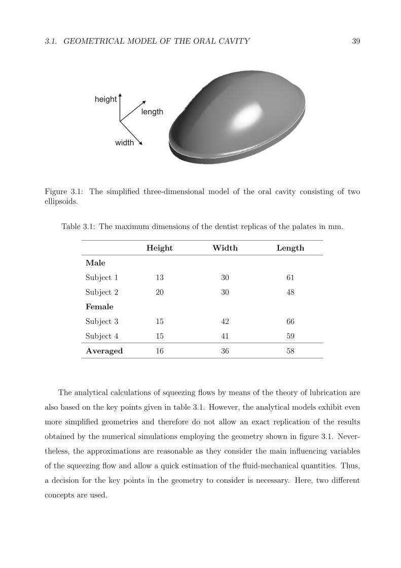
3.1. GEOMETRICAL MODEL OF THE ORAL CAVITY 39
height
length
width
Figure 3.1: The simplified three-dimensional model of the oral cavity consisting of twoellipsoids.
Table 3.1: The maximum dimensions of the dentist replicas of the palates in mm.
Height Width Length
Male
Subject 1 13 30 61
Subject 2 20 30 48
Female
Subject 3 15 42 66
Subject 4 15 41 59
Averaged 16 36 58
The analytical calculations of squeezing flows by means of the theory of lubrication are
also based on the key points given in table 3.1. However, the analytical models exhibit even
more simplified geometries and therefore do not allow an exact replication of the results
obtained by the numerical simulations employing the geometry shown in figure 3.1. Never-
theless, the approximations are reasonable as they consider the main influencing variables
of the squeezing flow and allow a quick estimation of the fluid-mechanical quantities. Thus,
a decision for the key points in the geometry to consider is necessary. Here, two different
concepts are used.
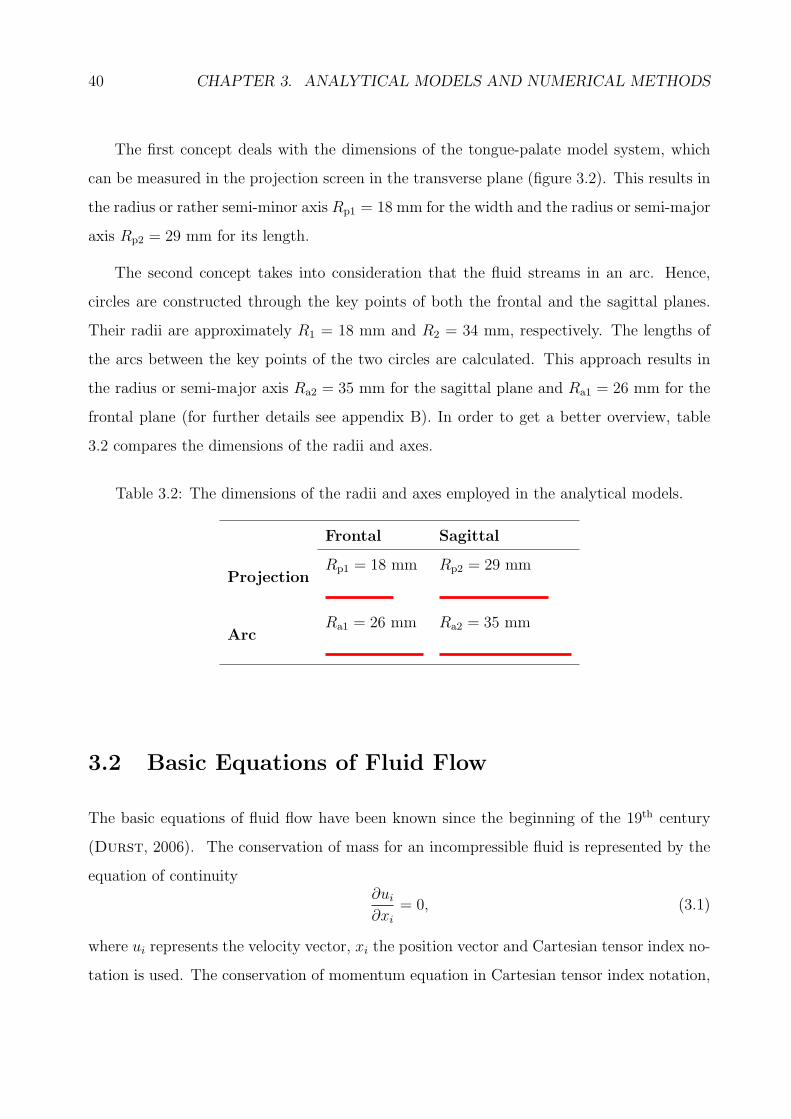
40 CHAPTER 3. ANALYTICAL MODELS AND NUMERICAL METHODS
The first concept deals with the dimensions of the tongue-palate model system, which
can be measured in the projection screen in the transverse plane (figure 3.2). This results in
the radius or rather semi-minor axis Rp1 = 18 mm for the width and the radius or semi-major
axis Rp2 = 29 mm for its length.
The second concept takes into consideration that the fluid streams in an arc. Hence,
circles are constructed through the key points of both the frontal and the sagittal planes.
Their radii are approximately R1 = 18 mm and R2 = 34 mm, respectively. The lengths of
the arcs between the key points of the two circles are calculated. This approach results in
the radius or semi-major axis Ra2 = 35 mm for the sagittal plane and Ra1 = 26 mm for the
frontal plane (for further details see appendix B). In order to get a better overview, table
3.2 compares the dimensions of the radii and axes.
Table 3.2: The dimensions of the radii and axes employed in the analytical models.
Frontal Sagittal
ProjectionRp1 = 18 mm Rp2 = 29 mm
ArcRa1 = 26 mm Ra2 = 35 mm
3.2 Basic Equations of Fluid Flow
The basic equations of fluid flow have been known since the beginning of the 19th century
(Durst, 2006). The conservation of mass for an incompressible fluid is represented by the
equation of continuity∂ui∂xi
= 0, (3.1)
where ui represents the velocity vector, xi the position vector and Cartesian tensor index no-
tation is used. The conservation of momentum equation in Cartesian tensor index notation,
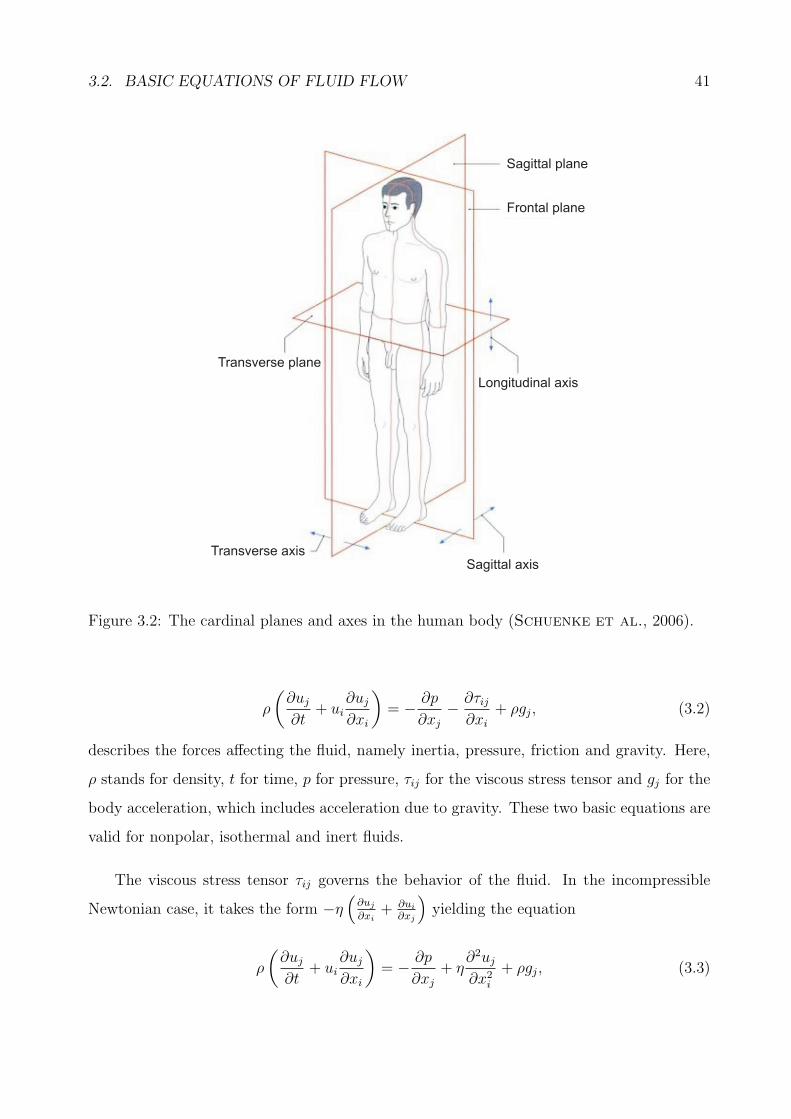
3.2. BASIC EQUATIONS OF FLUID FLOW 41
Sagittal plane
Frontal plane
Longitudinal axis
Sagittal axisTransverse axis
Transverse plane
Figure 3.2: The cardinal planes and axes in the human body (Schuenke et al., 2006).
ρ
(∂uj∂t
+ ui∂uj∂xi
)= − ∂p
∂xj− ∂τij∂xi
+ ρgj, (3.2)
describes the forces affecting the fluid, namely inertia, pressure, friction and gravity. Here,
ρ stands for density, t for time, p for pressure, τij for the viscous stress tensor and gj for the
body acceleration, which includes acceleration due to gravity. These two basic equations are
valid for nonpolar, isothermal and inert fluids.
The viscous stress tensor τij governs the behavior of the fluid. In the incompressible
Newtonian case, it takes the form −η(
∂uj
∂xi+ ∂ui
∂xj
)yielding the equation
ρ
(∂uj∂t
+ ui∂uj∂xi
)= − ∂p
∂xj+ η
∂2uj∂x2i
+ ρgj, (3.3)
42 CHAPTER 3. ANALYTICAL MODELS AND NUMERICAL METHODS
which is called the Navier-Stokes equation. From the non-Newtonian point of view,
several material laws representing distinct characteristics of fluid flow can be modeled using
different forms of τij. The decision of which one is to be used is based on the experimental
data and on which model fits best.
Yogurt was chosen to be the example food for the current study. It features a complex
internal microstructure consisting of a gel structure of milk proteins and fat molecules. This
structure is irreversibly damaged by increasing temperature and applying shear. Addition-
ally, the rheological behavior of yogurt is time dependent. Many different models have been
employed to describe its response to shear and stress (Mullineux & Simmons, 2008).
The three most common models that are used to describe the rheology of food in general
are the power law with an occurence of 47%, the Herschel-Bulkley model (20%) and, with a
frequency of 15%, the Casson model (Holdsworth, 1993). One drawback of these models
is that they are not suitable over a wide ranges of shear rates as they all give large values for
the viscosity η at low shear rates. Although not commonly used, the Crossmodel eliminates
this disadvantage and can successfully be applied over a wide range of shear rates (Cross,
1965, Geraghty & Butler, 1999, Mullineux & Simmons, 2008).
The appropriateness of the Crossmodel for stirred commercial yogurt has been reported
by Krulis & Rohm (2004). Their measurements were carried out by using a four-bladed
vane tool and a stress-controlled rheometer. Figure 3.3 shows the very low shear stresses
that occur at very low shear rates. The authors successfully applied the Cross model to
these measurements. This observation substantiates the assumption of Barnes &Walters
(1985) that materials only appear to exhibit yield stress because it is so difficult to measure
flows with low shear rates. For this reason, the Cross law is employed in the non-Newtonian
numerical simulation of the current study.
The Cross model was developed on the basis of molecular considerations. The model
follows the assumption that the average group size of flocculated interlinked particles is
dependent on the magnitude of the applied shear. The higher the shear rate, the lower the
rate of linkage becomes resulting in a limiting viscosity η∞ at the point of no linkage. The
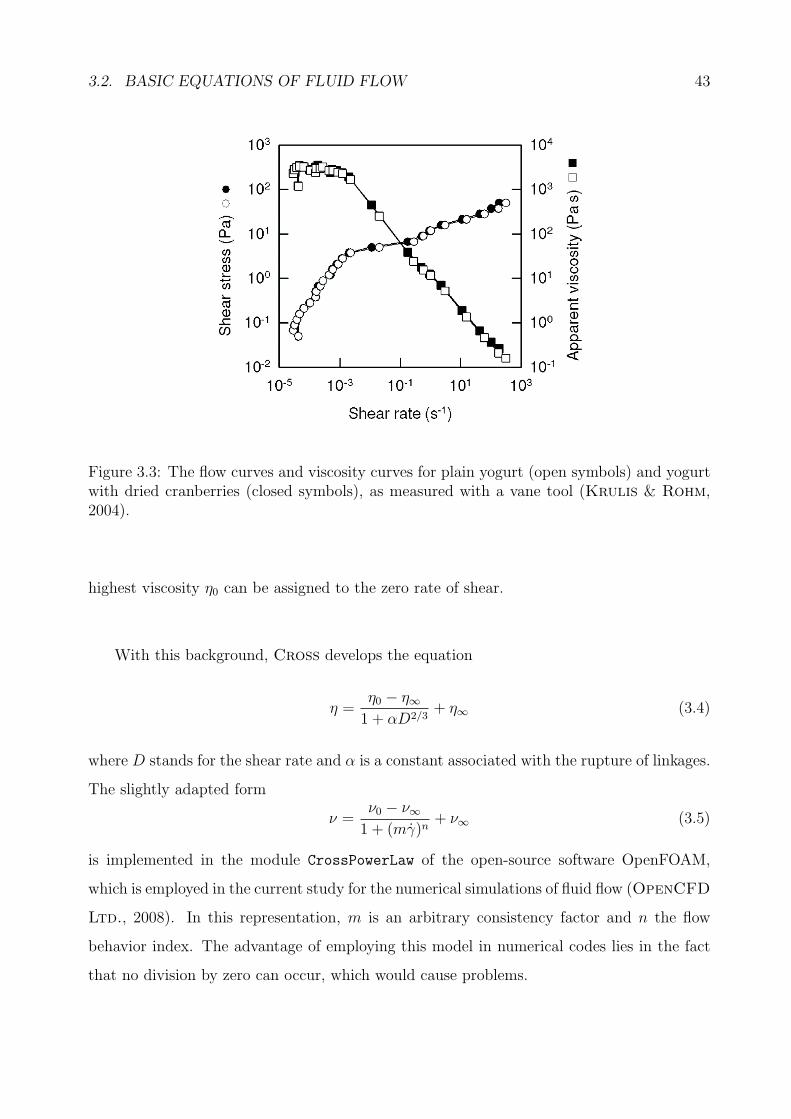
3.2. BASIC EQUATIONS OF FLUID FLOW 43
Figure 3.3: The flow curves and viscosity curves for plain yogurt (open symbols) and yogurtwith dried cranberries (closed symbols), as measured with a vane tool (Krulis & Rohm,2004).
highest viscosity η0 can be assigned to the zero rate of shear.
With this background, Cross develops the equation
η =η0 − η∞1 + αD2/3
+ η∞ (3.4)
where D stands for the shear rate and α is a constant associated with the rupture of linkages.
The slightly adapted form
ν =ν0 − ν∞
1 + (mγ)n+ ν∞ (3.5)
is implemented in the module CrossPowerLaw of the open-source software OpenFOAM,
which is employed in the current study for the numerical simulations of fluid flow (OpenCFD
Ltd., 2008). In this representation, m is an arbitrary consistency factor and n the flow
behavior index. The advantage of employing this model in numerical codes lies in the fact
that no division by zero can occur, which would cause problems.
44 CHAPTER 3. ANALYTICAL MODELS AND NUMERICAL METHODS
3.3 Theory of Lubrication
The theory of lubrication is based on Reynolds’ classic paper from 1886. It deals with
the behavior of thin Newtonian fluid films between two movable close surfaces. In various
technical applications, this approach helps to prevent damage occurring to surfaces due to
their sliding against each other (Cameron, 1966). On the occasion of the centennial of
Reynolds’s paper, Pinkus (1987) published an overview of the historical developments in
the theory of lubrication.
Due to the technical relevance of non-Newtonian fluid flow behavior the theory has been
expanded over the years. There have been several attempts to derive generalized Reynolds
equations for any kind of fluid-flow behavior, see for example Bourgin, Francois & Gay
(1985), Najji, Bousaid & Berthe (1989), Peiran & Shizhu (1990), Wolff & Kubo
(1996). In contrast to the approaches for Newtonian fluids derived by Reynolds, these
equations can no longer be solved analytically.
In bioengineering, the theory of lubrication obtained importance in respect of squeezing
films. Numerous research papers deal with the lubrication phenomena in human or animal
joints, for example Unsworth, Dowson & Wright (1975). Only recently, Tanaka, De-
tamore, Tanimoto & Kawai (2008) published a review article concerning the lubrication
of the temporomandibular joint. These investigations make it possible to reconstruct joints
or implant artificial joints after accidents.
In the context of the present thesis, the theory of lubrication is used in another aspect of
bioengineering. Four different geometrical models that mimic the squeezing flow in the oral
cavity in a greatly simplified way are derived. The simplest geometrical model consisting of
two plane circular parallel plates is well accepted in literature as a tongue-palate model. The
further models are used for the first time to model squeezing flow in the oral cavity and are
meant to discover the influence of different geometries, which are closer to the real geometry
in the human mouth. Therefore, the basic Reynolds equations for Newtonian fluid flow
behavior adapted to different coordinate systems are reduced according to the consideration
of a pure squeezing flow. These equations facilitate the calculation of the distributions of

3.3. THEORY OF LUBRICATION 45
different physical quantities in different geometrical configurations.
The theory of lubrication is based on some major assumptions (Cameron, 1966,Meyer,
2003). These are
• Newtonian fluid
• neglect of fluid inertia and body forces
• constant viscosity and pressure throughout the fluid film
• negligible velocity gradients apart from those in the cross-film direction
• no slip at the boundaries and
• laminar flow.
3.3.1 Reynolds Equation
Reynolds (1886) developed his equation on the basis of a streamed control cuboid in
a Cartesian coordinate system (figure 3.4). The thin Newtonian fluid film of height h is
located between two movable surfaces in the xy-plane. Their motion with velocities w0 and
wh in z-direction is followed by volume changes of the control cuboid. Additionally, these
surfaces are movable in parallel to the xy-plane with velocities u0 and uh in x-direction
and with velocities v0 and vh in y-direction. These movements are not followed by volume
changes of the control cuboid. For clarity, these velocities are not plotted in figure 3.4.
The fluid flow with the velocities u and v takes place in the yz- and the xz-planes,
respectively. The fluid exits through the same planes displaced by dx and dy with velocities
differing by dudxdx and dv
dydy.
Fluid Flow Velocities u and v
When dealing with lubrication, it is assumed that fluid inertia can be neglected, as the inertia
force is small compared to the viscous force, and also that body forces can be neglected. As a
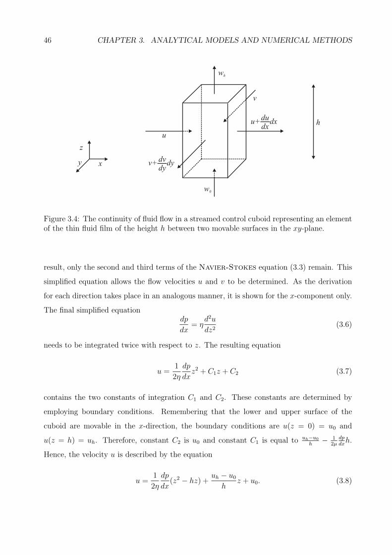
46 CHAPTER 3. ANALYTICAL MODELS AND NUMERICAL METHODS
u+ dxdudx
v+ dydvdy
u
v
wh
w0
h
z
xy
Figure 3.4: The continuity of fluid flow in a streamed control cuboid representing an elementof the thin fluid film of the height h between two movable surfaces in the xy-plane.
result, only the second and third terms of the Navier-Stokes equation (3.3) remain. This
simplified equation allows the flow velocities u and v to be determined. As the derivation
for each direction takes place in an analogous manner, it is shown for the x-component only.
The final simplified equationdp
dx= η
d2u
dz2(3.6)
needs to be integrated twice with respect to z. The resulting equation
u =1
2η
dp
dxz2 + C1z + C2 (3.7)
contains the two constants of integration C1 and C2. These constants are determined by
employing boundary conditions. Remembering that the lower and upper surface of the
cuboid are movable in the x-direction, the boundary conditions are u(z = 0) = u0 and
u(z = h) = uh. Therefore, constant C2 is u0 and constant C1 is equal to uh−u0
h− 1
2µdpdxh.
Hence, the velocity u is described by the equation
u =1
2η
dp
dx(z2 − hz) +
uh − u0h
z + u0. (3.8)
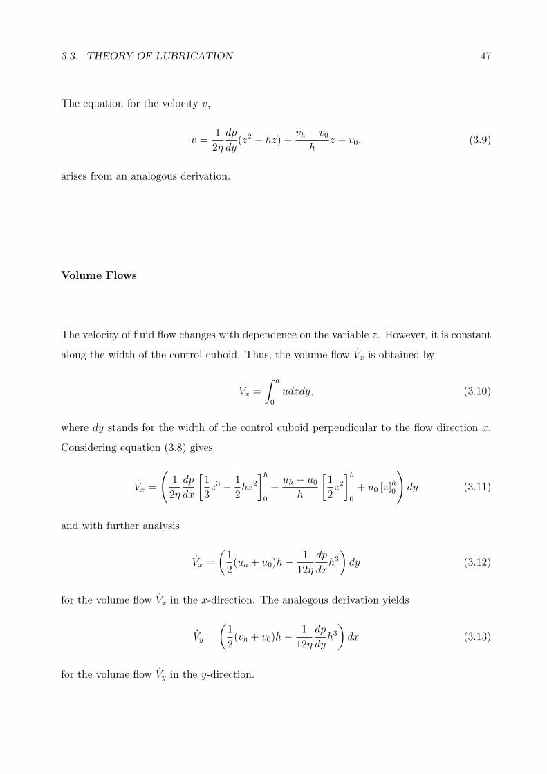
3.3. THEORY OF LUBRICATION 47
The equation for the velocity v,
v =1
2η
dp
dy(z2 − hz) +
vh − v0h
z + v0, (3.9)
arises from an analogous derivation.
Volume Flows
The velocity of fluid flow changes with dependence on the variable z. However, it is constant
along the width of the control cuboid. Thus, the volume flow Vx is obtained by
Vx =
∫ h
0
udzdy, (3.10)
where dy stands for the width of the control cuboid perpendicular to the flow direction x.
Considering equation (3.8) gives
Vx =
(1
2η
dp
dx
[1
3z3 − 1
2hz2]h0
+uh − u0
h
[1
2z2]h0
+ u0 [z]h0
)dy (3.11)
and with further analysis
Vx =
(1
2(uh + u0)h− 1
12η
dp
dxh3)dy (3.12)
for the volume flow Vx in the x-direction. The analogous derivation yields
Vy =
(1
2(vh + v0)h− 1
12η
dp
dyh3)dx (3.13)
for the volume flow Vy in the y-direction.
48 CHAPTER 3. ANALYTICAL MODELS AND NUMERICAL METHODS
Equation of Continuity
For the streamed volume element, without sources and sinks, considered here, the equation
of continuity must be valid. Assuming a fluid of constant density ρ, the rate of volume flow
must be constant. This brings
Vx + Vy + w0dxdy =
(Vx +
dVxdx
dx
)+
(Vy +
dVydy
dy
)+ whdxdy (3.14)
by employing the velocities w0 and wh for the velocities of the upper and lower surfaces in
the z-direction. Equivalent transformation gives
dVxdxdy
+dVydxdy
+ (wh − w0) = 0, (3.15)
taking into account a division by the area dxdy.
Reynolds Equation
The equation
d
dx
(1
2(uh + u0)h− 1
12η
dp
dxh3)+
d
dy
(1
2(vh + v0)h− 1
12η
dp
dyh3)+ (wh − w0) = 0 (3.16)
arises from substituting the volume flows Vx and Vy in equation (3.15) by the relationships
deduced in equations 3.12 and 3.13. Factorizing gives
d
dx
(h3dp
dx
)+
d
dy
(h3dp
dy
)= 6η
(d
dx((uh + u0)h) +
d
dy((vh + v0)h) + 2(wh − w0)
), (3.17)
which is named the Reynolds equation. As only one plate is moved in most cases, the
variable names of the velocities in the x- and y-direction, which are not zero, are replaced
by u and v. Thus, the simplified Reynolds equation,
d
dx
(h3dp
dx
)+
d
dy
(h3dp
dy
)= 6η
(d
dx(uh) +
d
dy(vh) + 2(wh − w0)
), (3.18)
3.3. THEORY OF LUBRICATION 49
is the starting point for analyzing the fluid flow in lubricating films.
Reynolds Equation in Cylindrical Coordinates
The Reynolds equation in cylindrical coordinates can be developed from the Reynolds
equation (3.18) in Cartesian coordinates. The relations
x = r cosφ, y = r sinφ and r2 = x2 + y2 (3.19)
are used for this transformation. This gives
1
r
d
dr
(rh3
dp
dr
)+
1
r2d
dφ
(h3dp
dφ
)=
6η
((u cosφ+ v sinφ)
dh
dr+ (−u sinφ+ v cosφ)
1
r
dh
dφ+
d
dφ(hω) + 2(wh − w0)
),
(3.20)
where ω is the angular velocity of the surface in the xy-plane (Cameron, 1966).
Reynolds Equation in Spherical Coordinates
Meyer (2003) derived the Reynolds equation in spherical coordinates. For this purpose,
a sphere of radius Ri lies in a hemispherical shell of the radius R and can be tilted by the
angle ψ with respect to the xy-plane. She obtained the equation
1
sin θ
d
dθ
(h3 sin θ
dp
dθ
)+
1
sin2 θ
d
dϕ
(h3dp
dϕ
)=
6R2η
(ω cosψ sinϕ
dh
dθ+
(ω sinψ + ω cosψ
cos θ
sin θcosϕ
)dh
dϕ+ 2
dh
dt
),
(3.21)
where θ is the zenith angle from the positive z-axis, ϕ is the azimuth angle from the positive
x-axis in the xy-plane and ω is the angular velocity vector of the inner sphere. As there is
no need for an inclination angle ψ in the present study, the equation
h = c− ex cosϕ sin θ − ey sin θ sinϕ− ez cos θ (3.22)
50 CHAPTER 3. ANALYTICAL MODELS AND NUMERICAL METHODS
derived by Goenka & Booker (1980) is adequate for the expression of the film thickness h.
Here, c stands for the radial clearance R − Ri, while ex, ey and ez are the eccentricities in
the different coordinate directions.
3.3.2 Squeezing Flow
Pure squeezing flows are characterized by exclusive motions of the surfaces in the z-direction.
There are neither relative motions in the x- and y-direction, nor rotational motions with the
angles φ, ϕ and θ. Simplifying the Reynolds equation (3.18) in Cartesian coordinates
according to these requirements gives
d
dx
(h3dp
dx
)+
d
dy
(h3dp
dy
)= 12η(wh − w0) (3.23)
for the description of a squeezing flow between two surfaces.
In the following derivations the lower surface is assumed to be fixed. In contrast, the
upper surface moves down with a uniform velocity. That means that the film thickness h
diminishes with the time t. The equation
d
dx
(h3dp
dx
)+
d
dy
(h3dp
dy
)= −12η
dh
dt(3.24)
depicts the resulting squeezing flow.
Analogously, the equations for the squeezing flow are
1
r
d
dr
(rh3
dp
dr
)= −12η
dh
dt(3.25)
in cylindrical coordinates and
d
dθ
(h3 sin θ
dp
dθ
)= 12R2η
dh
dtsin θ (3.26)
in spherical ones. The change in the algebraic sign arises from the fact that in the present
3.3. THEORY OF LUBRICATION 51
consideration the sphere is the movable component shifting against the upper hemisphere.
Applying these equations, the geometrical arrangements of both surfaces and the fluid
film between the two surfaces are variable in their shape. The oldest paper from Stefan
(1874) deals with a fluid film thickness h, which is constant along the radial coordinate r of
the circular plane plates. This approach is often used as a reference in food science, as has
been shown in the analytical approaches of section 2.2.4.
Reynolds (1886) derived a solution for the pressure distribution between two plane
elliptic plates. This approach is introduced here, as the projection plane of the numerical
model is elliptic.
Later attempts also investigated the fluid flow behavior due to a varying film thickness h
along the radius r of circular plates. In order to mimic the increasing fluid-film thickness,
which can be found in the numerical model, a double exponential function is employed. This
approach was first published by Murti in 1975.
Based on the previously introduced Reynolds equation in spherical coordinates it is
possible to derive equations describing the fluid flow along θ between a sphere and a hemi-
sphere. This approach reflects the three-dimensional nature of the human oral cavity simu-
lated in the numerical calculations.
All of the approaches introduced above belong to the few exceptions that are solvable
analytically. There are some cases in which a semi-analytical solution is appropriate. One
example is the squeezing flow in a journal bearing (Khonsari & Booser, 2001). Here, a
function for the fluid-film thickness h can be obtained. However, substituting the fluid-film
thickness h in the Reynolds equation by this function requires further numerical treatment
of the equation.
3.3.3 Plane Circular Parallel Plates - Stefan Equation
Figure 3.5 shows the geometrical arrangement of the two plane circular parallel plates em-
ployed by Stefan (1874). As the fluid film thickness h is constant along the radius r, it is
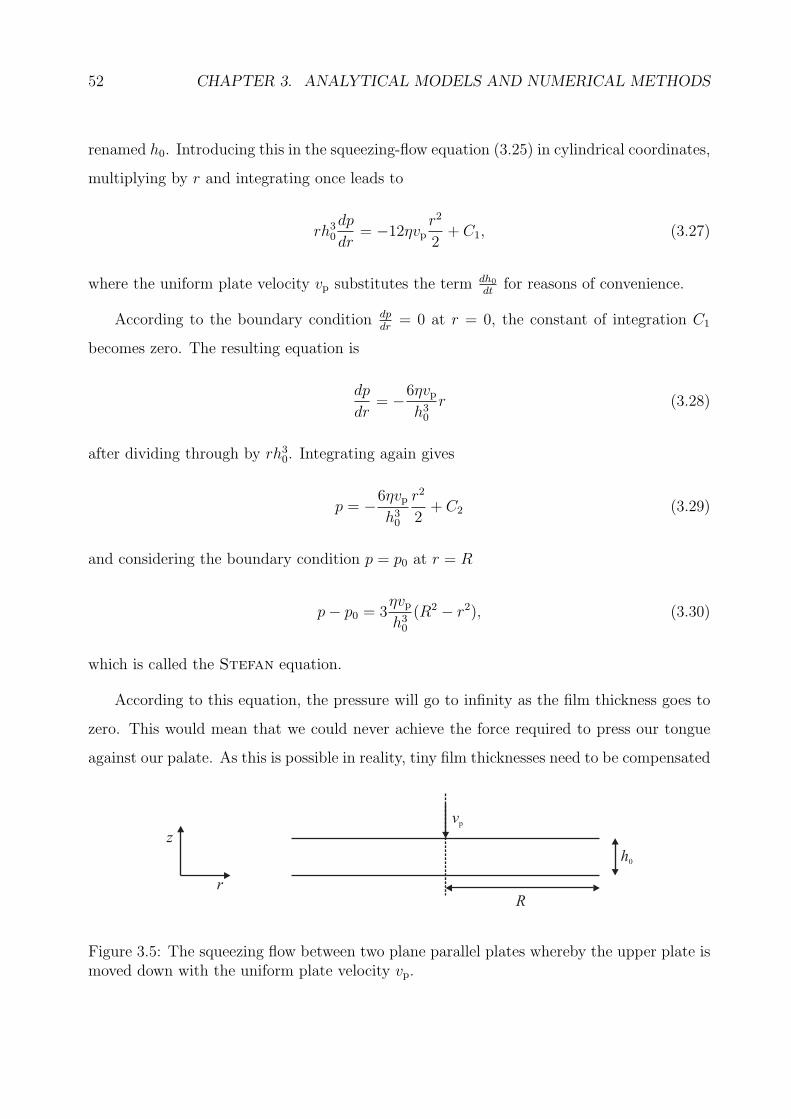
52 CHAPTER 3. ANALYTICAL MODELS AND NUMERICAL METHODS
renamed h0. Introducing this in the squeezing-flow equation (3.25) in cylindrical coordinates,
multiplying by r and integrating once leads to
rh30dp
dr= −12ηvp
r2
2+ C1, (3.27)
where the uniform plate velocity vp substitutes the term dh0
dtfor reasons of convenience.
According to the boundary condition dpdr
= 0 at r = 0, the constant of integration C1
becomes zero. The resulting equation is
dp
dr= −6ηvp
h30r (3.28)
after dividing through by rh30. Integrating again gives
p = −6ηvph30
r2
2+ C2 (3.29)
and considering the boundary condition p = p0 at r = R
p− p0 = 3ηvph30
(R2 − r2), (3.30)
which is called the Stefan equation.
According to this equation, the pressure will go to infinity as the film thickness goes to
zero. This would mean that we could never achieve the force required to press our tongue
against our palate. As this is possible in reality, tiny film thicknesses need to be compensated
z
r
R
h0
vp
Figure 3.5: The squeezing flow between two plane parallel plates whereby the upper plate ismoved down with the uniform plate velocity vp.
3.3. THEORY OF LUBRICATION 53
by moving the tongue with smaller velocities the closer it comes to the palate. Hence, the
tongue velocity cannot be kept constant during the whole process of deglutition.
Knowing the pressure profile it is possible to derive the corresponding velocity distri-
bution. As the squeezing flow is axisymmetric, the equations are derived in cylindrical
coordinates yielding velocity components in the z- and r-directions.
Starting from the equation of continuity,
1
r
∂
∂r(rur) +
1
r
∂uφ∂φ
+∂uz∂z
= 0, (3.31)
the expression for ur can be derived first (Middleman, 1998, Engmann, Servais & Bur-
bidge, 2005). This equation reduces to
1
r
∂
∂r(rur) +
∂uz∂z
= 0 (3.32)
as the fluid flow is axisymmetric. At the surface of the plates, there can only be a velocity
component uz in the z-direction due to the no-slip condition. This assumption is valid along
the radial coordinate r. For that reason, the equation can be rearranged to
1
r
∂
∂r(rur) = −∂uz
∂z= f(z, t), (3.33)
where the partial differentiation ∂uz
∂zis only a function f of the direction z and the time t.
In the next step, this result is substituted in the conservation of momentum equation. This
equation reads
∂p
∂r= η
(∂
∂r
(1
r
∂
∂r(rur)
)+
1
r2∂2ur∂φ2
− 2
r2∂uφ∂φ
+∂2ur∂z2
)(3.34)
in the r-direction considering only the dominant terms in lubrication theory, representing
pressure and friction, and can be reduced to
∂p
∂r= η
(∂
∂r
(1
r
∂
∂r(rur)
)+∂2ur∂z2
)(3.35)
54 CHAPTER 3. ANALYTICAL MODELS AND NUMERICAL METHODS
as a result of the axisymmetry. Inserting equation (3.33) yields
∂p
∂r= η
(∂
∂r(f(z, t)) +
∂2ur∂z2
)(3.36)
and∂p
∂r= η
∂2ur∂z2
(3.37)
respectively, as the function f(z, t) is independent of the r-direction. Integrating twice with
respect to z results in
ur =1
2η
∂p
∂rz2 + C1z + C2 (3.38)
for the velocity component ur. Taking the no-slip condition into consideration, the boundary
conditions are ur(0) = 0 and ur(h0) = 0. From these values, the integration constants C1
and C2 can be determined with the results being
C2 = 0 (3.39)
and
C1 = − 1
2η
∂p
∂rh0. (3.40)
These values lead to the equation
ur =1
2η
∂p
∂rh0z
(z
h0− 1
)(3.41)
and after inserting equation (3.30) to
ur = 3vph20rz
(1− z
h0
)(3.42)
for the velocity component ur.
The second velocity component uz can be derived by means of the continuity equation
3.3. THEORY OF LUBRICATION 55
in cylindrical coordinates (3.32). The result is
1
r
∂
∂r
(3vph20r2z
(1− z
h0
))+∂uz∂z
= 0 (3.43)
substituting the relationship for the velocity component ur. This equation is simplified and
rearranged yielding∂uz∂z
= 6vph30z2 − 6
vph20z (3.44)
and integrating with respect to z
uz = 3vph20z2(2
3
z
h0− 1
)+ C1 (3.45)
for the velocity component uz. The boundary condition is uz(0) = 0. This condition yields
the result
C1 = 0 (3.46)
for the integration constant C1. Therefore, the final equation is
uz = 3vph20z2(2
3
z
h0− 1
)(3.47)
for the velocity component in z-direction. In contrast to the pressure distribution, the
velocity components are independent from both viscosity η and the geometrical dimension,
R, of the plates. Differentiation of the function shows that the maximum and minimum
velocity values are found at the surfaces of the plates and that the inflection point is in the
middle of the fluid film.
Starting from the equation (3.42) for the velocity component in main fluid-flow direc-
tion, ur, the shear rate can be derived by differentiating with respect to the coordinate z.
This yields the equationdurdz
= 3vph20r
(1− 2
z
h0
), (3.48)
which is only dependent on the constants vp and h0. The result is most interesting at the
56 CHAPTER 3. ANALYTICAL MODELS AND NUMERICAL METHODS
surfaces of the models as the mechanoreceptors receive the stimuli here. The results are
durdz
= 3vph20r (3.49)
for z = 0 anddurdz
= −3vph20r (3.50)
for z = h0. This means that the same absolute values of shear rate occur at the different
surfaces. The absolute value of the shear stress,
τzr = 3ηvph20
r
(1− 2
z
h0
), (3.51)
results from the multiplication of the absolute value of the shear rate with the viscosity η.
The external force F that is required to drive the plates together can be obtained by
integrating the normal stress τzz over the radial coordinate of the plates (Middleman, 1998).
The result reads
F = 2π
∫ R
0
τzzrdr (3.52)
and can be further simplified assuming a Newtonian fluid. The equation
τzz = p− 2η∂uz∂z
(3.53)
shows the components of the normal stress τzz. The viscous part of the total normal stress τzz
can be neglected as there cannot be a velocity in the z-direction at the resting surface. Hence,
the force can be described by the equation
F = 2π
∫ R
0
p(r)rdr (3.54)
in which p(r) can be replaced by equation (3.30). Therefore, the equation
F =3
2πηvph30
R4 (3.55)
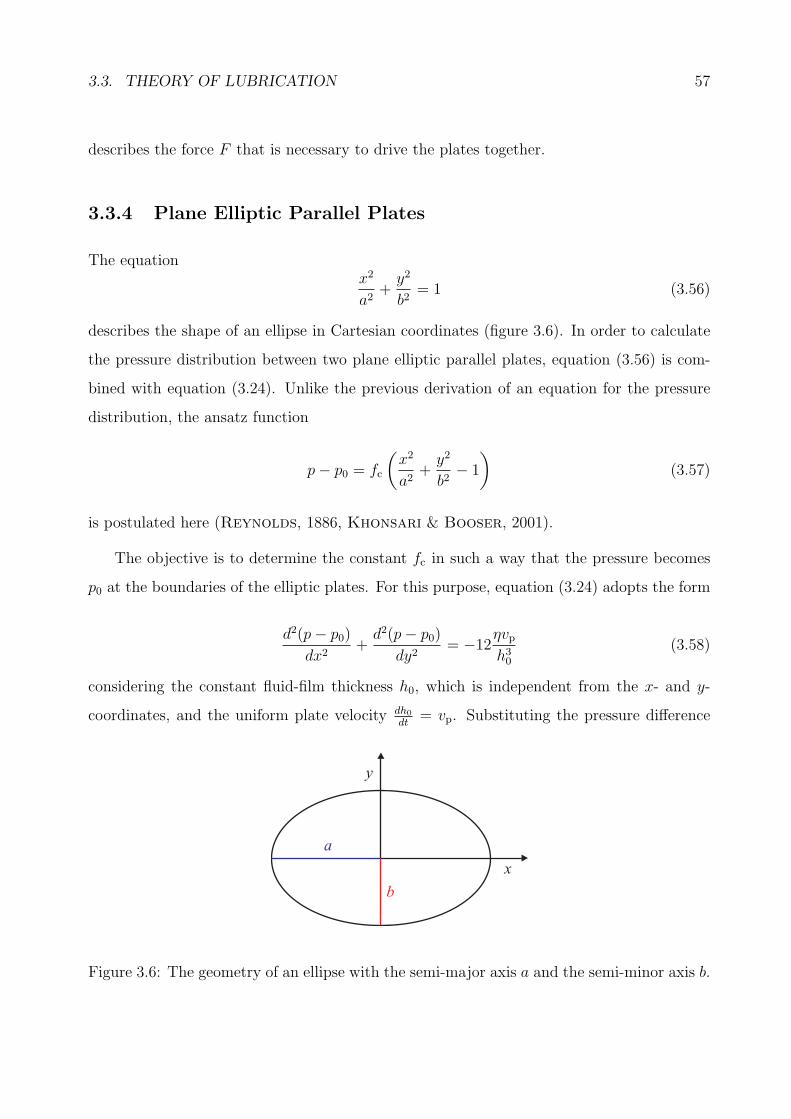
3.3. THEORY OF LUBRICATION 57
describes the force F that is necessary to drive the plates together.
3.3.4 Plane Elliptic Parallel Plates
The equationx2
a2+y2
b2= 1 (3.56)
describes the shape of an ellipse in Cartesian coordinates (figure 3.6). In order to calculate
the pressure distribution between two plane elliptic parallel plates, equation (3.56) is com-
bined with equation (3.24). Unlike the previous derivation of an equation for the pressure
distribution, the ansatz function
p− p0 = fc
(x2
a2+y2
b2− 1
)(3.57)
is postulated here (Reynolds, 1886, Khonsari & Booser, 2001).
The objective is to determine the constant fc in such a way that the pressure becomes
p0 at the boundaries of the elliptic plates. For this purpose, equation (3.24) adopts the form
d2(p− p0)
dx2+d2(p− p0)
dy2= −12
ηvph30
(3.58)
considering the constant fluid-film thickness h0, which is independent from the x- and y-
coordinates, and the uniform plate velocity dh0
dt= vp. Substituting the pressure difference
a
b
y
x
Figure 3.6: The geometry of an ellipse with the semi-major axis a and the semi-minor axis b.
58 CHAPTER 3. ANALYTICAL MODELS AND NUMERICAL METHODS
p− p0 by the ansatz function (3.57) yields
d2(
fa2x2)
dx2+d2(
fb2y2)
dy2= −12
ηvph30
(3.59)
and equivalent rearrangement
fc = −6ηvph30
a2b2
a2 + b2(3.60)
for the constant fc.
Therewith, the equation
p− p0 = −6ηvph30
a2b2
a2 + b2
(x2
a2+y2
b2− 1
)(3.61)
allows the calculation of the pressure distribution between two plane parallel elliptic plates.
In the next step, it is shown that the equation for the pressure distribution between two
parallel elliptic plates can be reduced to the one for plane circular parallel plates. This is the
case when both axes of the elliptic plates a and b are assumed to be equal to the radius R of
a circular plate. Furthermore, the Cartesian coordinates need to be rewritten in cylindrical
ones using x = r cosφ and y = r sinφ. Inserting these relationships in equation (3.61), the
result reads
p− p0 = −6ηvph30
R4
R2 +R2
((r cosφ)2
R2+
(r sinφ)2
R2− 1
). (3.62)
When simplified, this yields
p− p0 = −3ηvph30
R2
(r2(cos2 φ+ sin2 φ)−R2
R2
)(3.63)
and
p− p0 = 3ηvph30
(R2 − r2
), (3.64)
taking into account that cos2 φ+sin2 φ = 1. As this equation is the same as the equation for
a circular system, this shows that the two models [equations (3.30) and (3.61)] are consistent.
The starting point for the derivation of the equation representing the velocity compo-
3.3. THEORY OF LUBRICATION 59
nent ux is equation (3.6). The pressure gradient dpdx
can also be expressed by differentiating
equation (3.61) with respect to x. The equation
∂2ux∂z2
= −12vph30
b2
a2 + b2x (3.65)
arises from both relations. Integrating twice with respect to z yields
ux = −6vph30
b2
a2 + b2xz2 + C1z + C2 (3.66)
for the velocity component ux. The boundary conditions of the system are ux(0) = 0 and
ux(h0) = 0 yielding
C2 = 0 (3.67)
and
C1 = 6vph30
b2
a2 + b2xh0 (3.68)
for the integration constants C1 and C2. Inserting these constants leads to the final equation
ux = 6vph20
b2
a2 + b2xz
(1− z
h0
)(3.69)
for the velocity component ux. The equation
uy = 6vph20
a2
a2 + b2yz
(1− z
h0
)(3.70)
for the velocity component uy can be derived in an analogous manner.
The velocity component uz can be derived from the equation of continuity in Cartesian
coordinates [equation (3.1)]. Inserting the velocity components ux and uy yields the equation
∂uz∂z
= −6vph20z
(1− z
h0
), (3.71)
which was determined in the previous section. Therefore, the final expression for the velocity
component uz is the same as equation (3.47). This result is not surprising as the equation
60 CHAPTER 3. ANALYTICAL MODELS AND NUMERICAL METHODS
is independent of the coordinates of the main fluid-flow direction and only dependent on z.
Both geometrical configurations are similar in the z-direction due to the constant height of
the gap between the plane plates.
The shear rate can be calculated by differentiating the equations of velocity (3.69) and
(3.70) with respect to z. The equations
duxdz
= 6vph20
b2
a2 + b2x
(1− 2
z
h0
)(3.72)
andduydz
= 6vph20
a2
a2 + b2y
(1− 2
z
h0
)(3.73)
show the result. The most interesting shear rates are those at the surfaces of the geometry,
where z = 0 and z = h0, which are the wall shear stresses. These are
duxdz
= 6vph20
b2
a2 + b2x (3.74)
andduydz
= 6vph20
a2
a2 + b2y (3.75)
considering only their absolute values. Multiplying those equations with the viscosity η gives
the shear stress. The resulting equations read
τzx = 6ηvph20
b2
a2 + b2x
(1− 2
z
h0
)(3.76)
for the x-component and
τzy = 6ηvph20
a2
a2 + b2y
(1− 2
z
h0
)(3.77)
for the y-component.
The force F that is necessary to drive the plates together can be calculated by integrating
over the ellipse (Lorentz & Schmidt, 1922). The y-values at the outflow for certain x-
3.3. THEORY OF LUBRICATION 61
values can be derived from the equation of the ellipse (3.56). The equation
y =
∣∣∣∣ ba√a2 − x2∣∣∣∣ (3.78)
shows the absolute values. The outermost values of x are a and −a. Therefore, the integral
F = −6ηvph30
a2b2
a2 + b2
∫ a
−a
∫ ba
√a2−x2
− ba
√a2−x2
(x2
a2+y2
b2− 1
)dxdy (3.79)
leads to the final expression
F = 3πηvph30
a3b3
a2 + b2. (3.80)
This equation can directly be transformed into equation (3.55) considering a = b = R.
3.3.5 Plane and Curved Circular Parallel Plates
Figure 3.7 depicts the geometrical configuration employed by Murti (1975). The fluid film
thickness h is expressed by the double exponential function
h = h0e−βr2 , (3.81)
which obviously changes along the radius r. The distance h0 stands for the closest distance
between the two plates. The thickness h of the lubrication film increases to hmax at the outer
radius R of the circular plates. The variable β stands for the curvature parameter. If β is
zero, the upper plate will be planar. In this case, the derivation in section 3.3.3 is valid.
Equation (3.25) adopts the form
1
r
d
dr
(rh30e
−3βr2 dp
dr
)= −12η
d
dt
(h0e
−βr2)
(3.82)
after insertion of the function representing the film thickness h. The curvature parameter β
and the radial coordinate r are not dependent on the time t. This leaves the derivative dh0
dt
on the right hand side, which is substituted by the uniform plate velocity vp. Multiplying
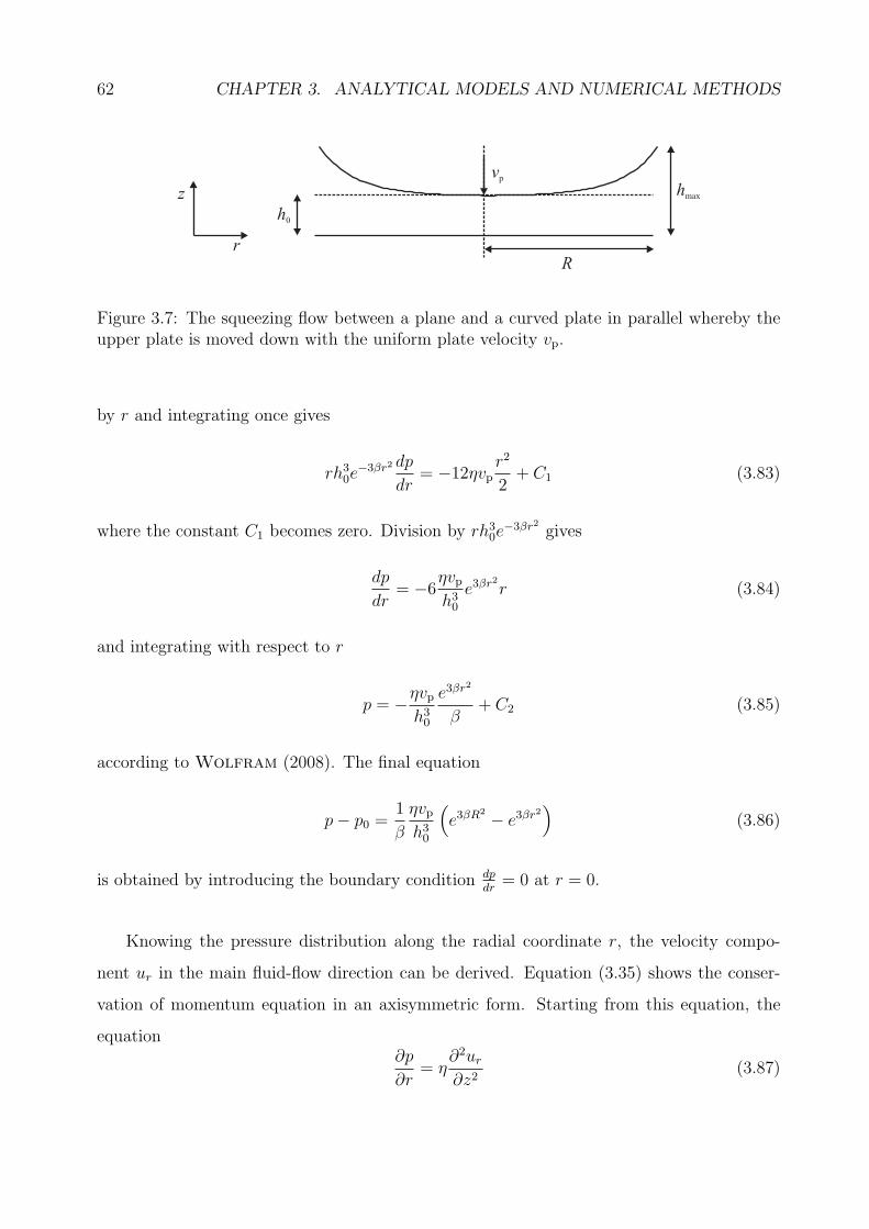
62 CHAPTER 3. ANALYTICAL MODELS AND NUMERICAL METHODS
hmaxz
r
R
h0
vp
Figure 3.7: The squeezing flow between a plane and a curved plate in parallel whereby theupper plate is moved down with the uniform plate velocity vp.
by r and integrating once gives
rh30e−3βr2 dp
dr= −12ηvp
r2
2+ C1 (3.83)
where the constant C1 becomes zero. Division by rh30e−3βr2 gives
dp
dr= −6
ηvph30
e3βr2
r (3.84)
and integrating with respect to r
p = −ηvph30
e3βr2
β+ C2 (3.85)
according to Wolfram (2008). The final equation
p− p0 =1
β
ηvph30
(e3βR
2 − e3βr2)
(3.86)
is obtained by introducing the boundary condition dpdr
= 0 at r = 0.
Knowing the pressure distribution along the radial coordinate r, the velocity compo-
nent ur in the main fluid-flow direction can be derived. Equation (3.35) shows the conser-
vation of momentum equation in an axisymmetric form. Starting from this equation, the
equation∂p
∂r= η
∂2ur∂z2
(3.87)
3.3. THEORY OF LUBRICATION 63
can be deduced from the assumption of lubrication theory that the gradient of the velocity
component ur in the r-direction is negligible. In the next step, the equation representing the
pressure distribution (3.86) needs to be obtained. The resulting equation
∂2ur∂z2
= −6vph30re3βr
2
(3.88)
is integrated twice with respect to z yielding
ur = −3vph30re3βr
2
z2 + C1z + C2 (3.89)
for the velocity component ur. Due to the no-slip condition the boundary conditions are
ur(z = 0) = 0 and ur(z = h0e−βr2) = 0. These give values of
C2 = 0 (3.90)
and
C1 = 3vph20re2βr
2
(3.91)
for the integration constants. Insertion of these values leads to the final equation
ur = 3vph20rze2βr
2
(1− z
h0eβr
2
)(3.92)
for the velocity component ur in the main fluid-flow direction.
The shear ratedurdz
= 3vph20re2βr
2
(1− 2
z
h0eβr
2
)(3.93)
can be derived by differentiating the velocity ur with respect to z. The absolute value of the
shear rate at the surfaces isdurdz
= 3vph20re2βr
2
(3.94)
64 CHAPTER 3. ANALYTICAL MODELS AND NUMERICAL METHODS
taking into account z = 0 and z = h0e−βr2 . The shear stress,
τzr = 3ηvph20
re2βr2
(1− 2
z
h0eβr
2
), (3.95)
is obtained by multiplying the shear rate with the viscosity η.
The force F that is required to move the plates together can be calculated by integration
again. The equation reads
F = 2π
∫ R
0
rp(r)dr (3.96)
and can be transformed into
F =1
3πηvpβ2h30
(e3βR
2
(e3βR2 − 1) + 1
)(3.97)
taking into account equation (3.86).
3.3.6 Sphere in a Hemisphere
On the basis of the given Reynolds equation (3.21) in spherical coordinates (Meyer, 2003)
an equation for a pure squeezing flow between a sphere and a hemisphere can be deduced.
This novel equation reflects the situation in the oral cavity best and is solvable analytically
with several simplifications. It is assumed that the inner sphere lies centric in the outer
hemisphere with regard to the x- and y-direction. Consequently, the resulting fluid flow
must be axially symmetric with respect to the z-axis (figure 3.8).
The Reynolds equation in spherical coordinates (3.21) can be simplified, resulting in
d
dθ
(h3 sin θ
dp
dθ
)= 12R2η
dh
dtsin θ (3.98)
considering the above defined restrictions for a pure squeezing flow. The equation (3.22) for
the film thickness h reduces to
h = c− ez cos θ (3.99)
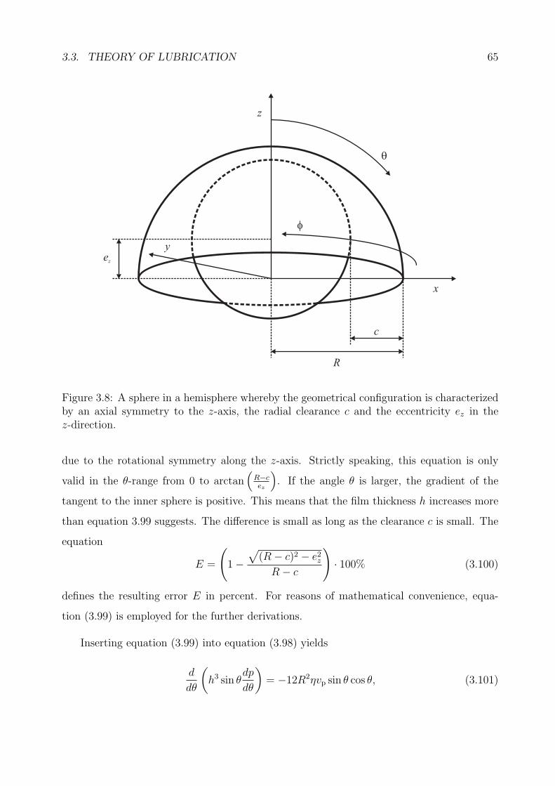
3.3. THEORY OF LUBRICATION 65
x
z
c
R
ez
f
q
y
Figure 3.8: A sphere in a hemisphere whereby the geometrical configuration is characterizedby an axial symmetry to the z-axis, the radial clearance c and the eccentricity ez in thez-direction.
due to the rotational symmetry along the z-axis. Strictly speaking, this equation is only
valid in the θ-range from 0 to arctan(
R−cez
). If the angle θ is larger, the gradient of the
tangent to the inner sphere is positive. This means that the film thickness h increases more
than equation 3.99 suggests. The difference is small as long as the clearance c is small. The
equation
E =
(1−
√(R− c)2 − e2zR− c
)· 100% (3.100)
defines the resulting error E in percent. For reasons of mathematical convenience, equa-
tion (3.99) is employed for the further derivations.
Inserting equation (3.99) into equation (3.98) yields
d
dθ
(h3 sin θ
dp
dθ
)= −12R2ηvp sin θ cos θ, (3.101)
66 CHAPTER 3. ANALYTICAL MODELS AND NUMERICAL METHODS
taking into account that only the eccentricity ez depends on the time and that the uniform
velocity dezdt
can be replaced by vp in analogy to the previous sections.
Integrating this equation results in
h3 sin θdp
dθ= −6R2ηvp sin
2 θ + C1 (3.102)
with C1 = 0 due to the boundary condition dpdθ
= 0 at θ = 0. Dividing through by h3 sin θ
and substituting h by equation (3.99) gives the equation
dp
dθ= − 6R2ηvp sin θ
(c− ez cos θ)3, (3.103)
which needs to be integrated again (Gradshteyn & Ryzhik, 1980). The result
p =3R2ηvp
ez(c− ez cos θ)2+ C2 (3.104)
contains the second constant of integration C2. This constant can be determined to be
C2 = p0 −3R2ηvpezc2
(3.105)
as the pressure becomes p0 at the angle θ = 90◦. The final equation is
p− p0 =3R2ηvpez
(1
(c− ez cos θ)2− 1
c2
)= 3R2ηvp
2c cos θ − ez cos2 θ
c2 (c− ez cos θ)2 , (3.106)
with the restrictions that both the radial clearance c and the film thickness h [see equa-
tion (3.99)] may be small but not zero.
In the next step, the velocity is derived. The conservation of momentum equation in
3.3. THEORY OF LUBRICATION 67
spherical coordinates reads
1
r
∂p
∂θ=
η
(1
r2∂
∂r
(r2∂uθ∂r
)+
1
r2∂
∂θ
(1
sin θ
∂
∂θ(uθ sin θ)
)+
1
r2 sin2 θ
∂2uθ∂ϕ2
+2
r2∂ur∂θ
− 2 cos θ
r2 sin2 θ
∂uϕ∂ϕ
)(3.107)
in its complete form in the θ-direction. This equation reduces to
1
r
∂p
∂θ= η
(1
r2∂
∂r
(r2∂uθ∂r
)+
1
r2∂
∂θ
(1
sin θ
∂
∂θ(uθ sin θ)
)+
2
r2∂ur∂θ
)(3.108)
due to axisymmetry. The main fluid-flow direction is the θ-direction. Again, the assumption
that the velocity gradient in this direction is negligible, is valid. This leads to the greatly
simplified equation∂p
∂θ= η
1
r
∂
∂r
(r2∂uθ∂r
), (3.109)
which features a comparable structure to the initial equations in the former sections. The
equation∂
∂r
(r2∂uθ∂r
)= −6vp
R2 sin θ
(c− ez cos θ)3r (3.110)
arises from inserting the pressure distribution given by equation (3.106). The following steps
are integration with respect to r, dividing by r2 and integration with respect to r again. This
leads to the equation
uθ = −3vpR2 sin θ
(c− ez cos θ)3r − C1
r+ C2 (3.111)
for the velocity component uθ in the main fluid-flow direction. The boundary conditions are
uθ(r = R) = 0 and uθ(r = R− c+ez cos θ) = 0. From these values, the integration constants
C1 = −3vpR3 sin θ
(c− ez cos θ)3((c− ez cos θ)−R) (3.112)
and
C2 = −3vpR2 sin θ
(c− ez cos θ)3((c− ez cos θ)− 2R) (3.113)
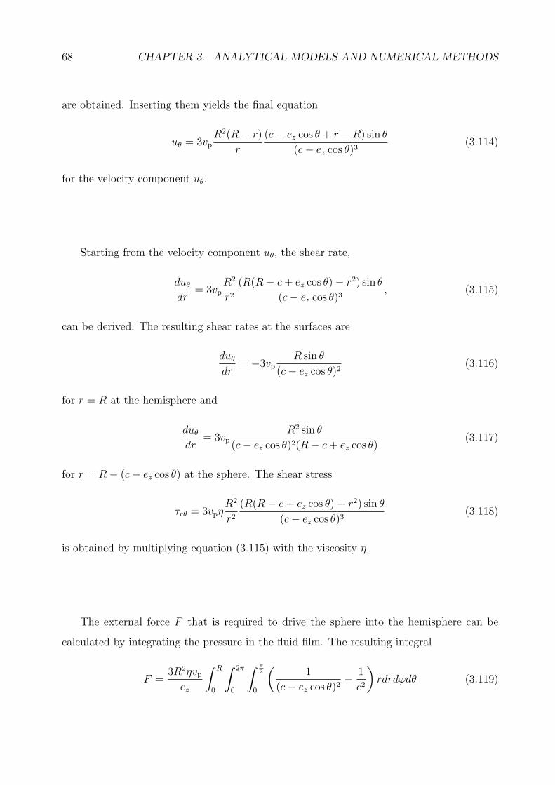
68 CHAPTER 3. ANALYTICAL MODELS AND NUMERICAL METHODS
are obtained. Inserting them yields the final equation
uθ = 3vpR2(R− r)
r
(c− ez cos θ + r −R) sin θ
(c− ez cos θ)3(3.114)
for the velocity component uθ.
Starting from the velocity component uθ, the shear rate,
duθdr
= 3vpR2
r2(R(R− c+ ez cos θ)− r2) sin θ
(c− ez cos θ)3, (3.115)
can be derived. The resulting shear rates at the surfaces are
duθdr
= −3vpR sin θ
(c− ez cos θ)2(3.116)
for r = R at the hemisphere and
duθdr
= 3vpR2 sin θ
(c− ez cos θ)2(R− c+ ez cos θ)(3.117)
for r = R− (c− ez cos θ) at the sphere. The shear stress
τrθ = 3vpηR2
r2(R(R− c+ ez cos θ)− r2) sin θ
(c− ez cos θ)3(3.118)
is obtained by multiplying equation (3.115) with the viscosity η.
The external force F that is required to drive the sphere into the hemisphere can be
calculated by integrating the pressure in the fluid film. The resulting integral
F =3R2ηvpez
∫ R
0
∫ 2π
0
∫ π2
0
(1
(c− ez cos θ)2− 1
c2
)rdrdφdθ (3.119)
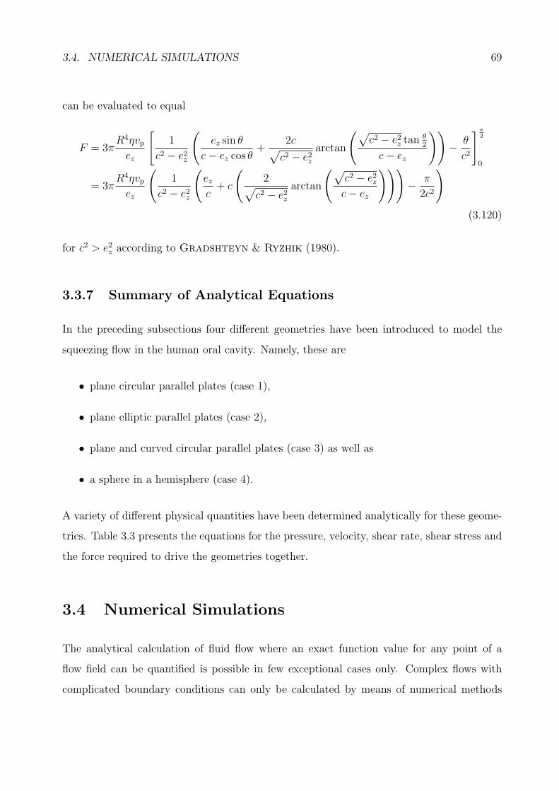
3.4. NUMERICAL SIMULATIONS 69
can be evaluated to equal
F = 3πR4ηvpez
[1
c2 − e2z
(ez sin θ
c− ez cos θ+
2c√c2 − e2z
arctan
(√c2 − e2z tan
θ2
c− ez
))− θ
c2
]π2
0
= 3πR4ηvpez
(1
c2 − e2z
(ezc+ c
(2√
c2 − e2zarctan
(√c2 − e2zc− ez
)))− π
2c2
)(3.120)
for c2 > e2z according to Gradshteyn & Ryzhik (1980).
3.3.7 Summary of Analytical Equations
In the preceding subsections four different geometries have been introduced to model the
squeezing flow in the human oral cavity. Namely, these are
• plane circular parallel plates (case 1),
• plane elliptic parallel plates (case 2),
• plane and curved circular parallel plates (case 3) as well as
• a sphere in a hemisphere (case 4).
A variety of different physical quantities have been determined analytically for these geome-
tries. Table 3.3 presents the equations for the pressure, velocity, shear rate, shear stress and
the force required to drive the geometries together.
3.4 Numerical Simulations
The analytical calculation of fluid flow where an exact function value for any point of a
flow field can be quantified is possible in few exceptional cases only. Complex flows with
complicated boundary conditions can only be calculated by means of numerical methods
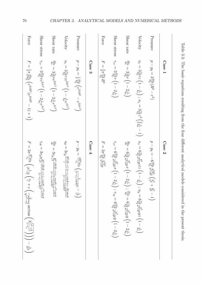
70 CHAPTER 3. ANALYTICAL MODELS AND NUMERICAL METHODSTab
le3.3:
Thebasic
equation
sresu
ltingfrom
thefou
rdifferen
tan
alytical
models
consid
eredin
thepresen
tthesis.
Case
1Case
2
Pressu
rep−p0=
3ηvp
h30(R
2−r2)
p−p0=
−6ηvp
h30
a2b2
a2+b2 (
x2
a2+
y2
b2−
1 )Velo
cityur=
3vp
h20 rz (
1−
zh0 )
;uz=
3vp
h20 z
2 (23
zh0 −
1 )ux=
6vp
h20
b2
a2+b2 xz (
1−
zh0 )
;uy=
6vp
h20
a2
a2+b2 yz (
1−
zh0 )
Shear
ratedur
dz=
3vp
h20 r (
1−
2zh0 )
dux
dz=
6vp
h20
b2
a2+b2 x (
1−2
zh0 )
;duy
dz=
6vp
h20
a2
a2+b2 y (
1−
2zh0 )
Shear
stressτzr=
3ηvp
h20r (
1−
2zh0 )
τzx=
6ηvp
h20
b2
a2+b2 x (
1−2
zh0 )
;τzy=
6ηvp
h20
a2
a2+b2 y (
1−
2zh0 )
Force
F=
32 πηvp
h30R
4F
=3π
ηvp
h30
a3b3
a2+b2
Case
3Case
4
Pressu
rep−p0=
1β
ηvp
h30 (
e3βR
2−e3βr2 )
p−p0=
3R
2ηvp
ez (
1(c−
ezco
sθ)2 −
1c2 )
Velo
cityur=
3vp
h20 rze
2βr2 (
1−
zh0 e
βr2 )
uθ=
3vpR
2(R
−r)
r(c−
ezco
sθ+r−
R)sin
θ(c−
ezco
sθ)3
Shear
ratedur
dz=
3vp
h20 re
2βr2 (
1−2
zh0 e
βr2 )
duθ
dr=
3vpR
2
r2
(R(R
−c+
ezco
sθ)−
r2)sin
θ(c−
ezco
sθ)3
Shear
stressτzr=
3ηvp
h20re
2βr2 (
1−2
zh0 e
βr2 )
τrθ=
3vp η
R2
r2
(R(R
−c+
ezco
sθ)−
r2)sin
θ(c−
ezco
sθ)3
Force
F=
13 πηvp
β2h30 (e3βR
2(e3βR
2−1)
+1 )
F=
3πR
4ηvp
ez (
1c2−
e2z (
ezc+c (
2√
c2−
e2z
arctan (√
c2−
e2z
c−ez )))
−π2c2 )
3.4. NUMERICAL SIMULATIONS 71
(Kowalczyk, Hartmann & Delgado, 2004, Hartmann, Mathmann & Delgado,
2006). Just as with analytical solutions, these calculations are always approximations of
reality. Nevertheless, they are helpful in order to visualize processes, which are difficult to
access.
The process of deglutition taking place isolated from any in vivo insight belongs to such
processes. There is no measurement system that can completely deal with the conditions of
the oral cavity, namely the wetness and the difficulty of fixing a system. For this reason,
numerical simulations offer the appropriate feasibility for studying the process.
Furthermore, numerical simulations offer
• more detailed information about the flow field,
• information about flow variables that are not measurable directly,
• the possibility to eliminate disturbance variables,
• a more flexible adaptation of input variables as well as
• the advantage of being less expensive and time consuming compared to experimental
set-ups
according to Bohme (2000). In computational fluid dynamics, the resulting partial differ-
ential equations are subsequently solved using the numerical code.
3.4.1 Procedure of a CFD Analysis
The procedure of a computational fluid dynamics (CFD) analysis starts with the preprocess-
ing. A grid is generated covering the whole geometrical domain of fluid flow. This entails a
division into discrete cells called control volumes. The basic equations of fluid flow are an
essential part of the selected discrete mathematical model, which is applied on the discrete
cells. The application of the model results in solutions for pressure and velocity in every
single discrete cell of the entire domain for every single time step. The solution for the entire
72 CHAPTER 3. ANALYTICAL MODELS AND NUMERICAL METHODS
domain is merged spatio-temporally based on the results for the single cells (Ferziger &
Peric, 2002). In the final step, the fluid flow is visualized by a postprocessor. This enables
analysis and interpretation of the numerical calculation.
3.4.2 Discretization Methods
The discretization step approximates the non-linear partial differential equations of fluid flow
by transferring them into a system of algebraic equations that can be solved iteratively taking
into account initial and boundary conditions. Hence, the function that is the analytical
solution of the partial differential equations is replaced by a finite amount of values at
discrete locations in space and time. This approximation is made for each small discrete
domain, either for each node, volume or element depending on the discretization method.
There are different strategies and algorithms for discretization methods. Ultimately, all
of them lead to the same solution for the entire flow field. Three methods have proved of value
and are the most important ones, namely the methods of finite differences, finite volumes and
finite elements. These methods are introduced concisely in the following. Other methods
like spectral schemes, boundary element methods and cellular automata are employed for
special classes of problems.
The finite difference method dates back to Leonhard Euler in the 18th century. It is
the simplest method for solving partial differential equations and is known to be applied on
structured grids only. The basic equations of fluid flow in their differential form as presented
above are solved at the grid nodes. For that purpose, the partial derivatives are substituted
by difference quotients resulting in a system of difference equations that can be solved by
means of implicit and explicit algorithms. Knorrenschild (2003) gives an overview of
appropriate algorithms.
The finite volume method is the most frequently used method in computational fluid
dynamics currently. The requirements regarding the grid structure are small, leading to the
application of more flexible unstructured grids. The finite volume method is based on the
3.4. NUMERICAL SIMULATIONS 73
basic equations of fluid flow in their integral form. The integrals are solved by approximations
in the centers of each finite volume.
The finite element method is comparable to the finite volume method in many aspects.
The main difference is that the equations are multiplied by a weight function, which is
defined within the elements before they are integrated over the entire domain.
3.4.3 Types of Grids
Discretization methods are applied on the basis of numerical grids. The grids split the entire
geometrical domain into a finite number of discrete locations. They can be structured or
unstructured.
The structured grid is the simplest grid structure. The regular grid is aligned along the
underlying coordinate system. The grid lines intersect only at the nodes. Therewith, each
element has a fixed number of neighbor elements and nodes. Structured grids can only be
employed for geometrically simple solution domains and are most frequently used with the
finite difference method. In some cases, the appropriate distribution of grid points can be
difficult.
On the contrary, unstructured grids are highly flexible for complex geometries. They can
have arbitrary shapes and no restrictions concerning the number of neighbor elements and
nodes. The most common element shapes are triangles and quadrilaterals in two-dimensional
domains and tetrahedra and hexahedra in three-dimensional domains. This grid technique
is best adapted to both the finite volume and element methods. The most important disad-
vantage of this kind of grid is the resulting irregularity of the data structure as the matrices
are no longer regular or diagonal.
3.4.4 Software
The numerical analysis of the current study is based on several softwares. Each step -
preprocessing, solver, postprocessing - needs its own tool. Due to better availability and
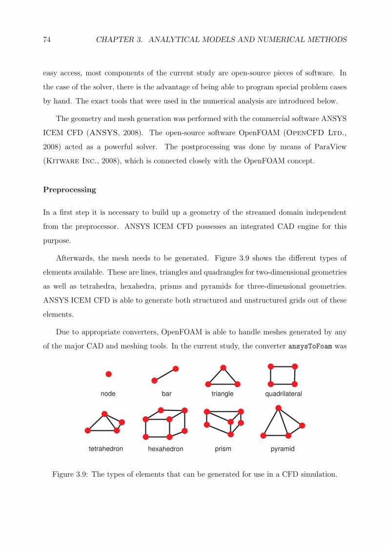
74 CHAPTER 3. ANALYTICAL MODELS AND NUMERICAL METHODS
easy access, most components of the current study are open-source pieces of software. In
the case of the solver, there is the advantage of being able to program special problem cases
by hand. The exact tools that were used in the numerical analysis are introduced below.
The geometry and mesh generation was performed with the commercial software ANSYS
ICEM CFD (ANSYS, 2008). The open-source software OpenFOAM (OpenCFD Ltd.,
2008) acted as a powerful solver. The postprocessing was done by means of ParaView
(Kitware Inc., 2008), which is connected closely with the OpenFOAM concept.
Preprocessing
In a first step it is necessary to build up a geometry of the streamed domain independent
from the preprocessor. ANSYS ICEM CFD possesses an integrated CAD engine for this
purpose.
Afterwards, the mesh needs to be generated. Figure 3.9 shows the different types of
elements available. These are lines, triangles and quadrangles for two-dimensional geometries
as well as tetrahedra, hexahedra, prisms and pyramids for three-dimensional geometries.
ANSYS ICEM CFD is able to generate both structured and unstructured grids out of these
elements.
Due to appropriate converters, OpenFOAM is able to handle meshes generated by any
of the major CAD and meshing tools. In the current study, the converter ansysToFoam was
node bar triangle quadrilateral
tetrahedron hexahedron prism pyramid
Figure 3.9: The types of elements that can be generated for use in a CFD simulation.

3.4. NUMERICAL SIMULATIONS 75
applied in order to transform the geometries and meshes into the format of OpenFOAM.
Solver
The principles of the open-source software OpenFOAM (Open Field Operation and Manip-
ulation) were introduced by Weller, Tabor, Jasak & Fureby (1998). OpenFOAM is a
numerical tool for solving partial differential equations of any kind. The solvers are based on
C++ modules. The wide range of solvers that are already implemented can be viewed on the
website. Emphasis is put on continuum mechanics including computational fluid mechan-
ics. The CFD codes are based on the finite volume method. The different problem-specific
solvers are grouped to the topics “basic” CFD codes, incompressible flow, compressible flow,
multiphase flow, direct numerical simulation and large eddy simulation, combustion, heat
transfer, electromagnetics, stress analysis of solids and even finance.
The solvers that belong to the group of incompressible flow are relevant for the current
study. In order to simulate Newtonian fluid flow, the solver icoDyMFoam was employed. This
solver allows the calculation of laminar and transient flows considering dynamic meshes. For
simulating the non-Newtonian fluid flow it was necessary to program a new solver. This
took place on the basis of the nonNewtonianIcoFoam solver, which supports the calculation
of laminar non-Newtonian and transient flow but not dynamic meshes. The new solver was
generated analogously to the icoDyMFoam solver. The developed nonNewtonianIcoDyMFoam
code can be found in appendix C. The solvers access the Newtonian module, which contains
a linear viscous fluid model, as well as CrossPowerLaw and BirdCarreau, which both contain
nonlinear viscous models.
The solvers output data in terms of pressure and velocity, as well as viscosity in the
non-Newtonian case. Additional modules of OpenFOAM are able to transfer these data into
the required gradients. The magU module calculates the scalar magnitude of the velocity
field ui at each time. Another useful module is magGradU, which calculates and writes the
scalar magnitude of the gradient of the velocity field ui for each time.
76 CHAPTER 3. ANALYTICAL MODELS AND NUMERICAL METHODS
Postprocessing
Once the necessary data are generated they are transformed into an appropriate format for
postprocessing. OpenFOAM features several data converters, which allow the subsequent
analysis by means of third party products like Fluent or EnSight. The converter used in the
current study is the foamToVTK converter. It converts data from its native format to the
VTK format. VTK (Visualization Toolkit) is a platform independent open-source graphics
toolkit. It is used by ParaView as a data-processing and rendering engine.
The ParaView open-source visualization application represents data in structured as well
as in unstructured grids. The software quickly builds visualizations of even extremely large
data sets so that they can be analyzed by qualitative and quantitative techniques. Therefore,
ParaView needs a list of the grid points with the associated data that is to be visualized.
These data are recorded in separate text files.
3.4.5 Introduction of the Geometrical Model
The current thesis continues the previous study of a two-dimensional numerical approach
(Mathmann, Kowalczyk, Petermeier, Baars, Eberhard & Delgado, 2007). The
aim of that study was to determine numerically the fluid-mechanical forces occurring in food
suspensions using a simplified tongue-palate model system consisting of two parallel plates.
The calculations by means of the Stefan equation proved the appropriateness of numerical
methods for the investigation of fluid flow in models of the oral cavity. Due to this validation
of the model consisting of two plane circular parallel plates, further comparisons of numeri-
cally and analytically calculated properties of squeezing flows for other geometries have not
been performed as it is very likely they will give identical results leading to redundant data.
Accordingly, the two-dimensional model used in the first numerical study has been extended
to a more complex three-dimensional model directly. However, this model can be considered
as the logical continuation of the geometrical models that are discussed analytically.
Figure 3.10 shows the geometry of the model based on the dentist replicas introduced
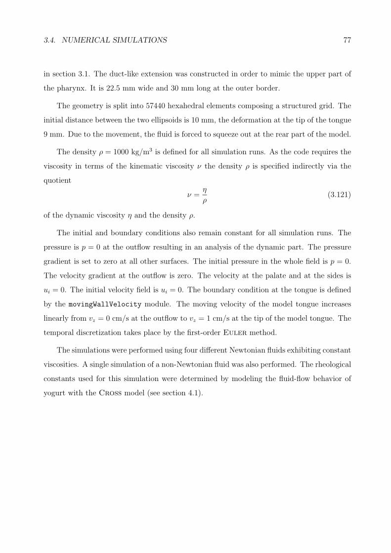
3.4. NUMERICAL SIMULATIONS 77
in section 3.1. The duct-like extension was constructed in order to mimic the upper part of
the pharynx. It is 22.5 mm wide and 30 mm long at the outer border.
The geometry is split into 57440 hexahedral elements composing a structured grid. The
initial distance between the two ellipsoids is 10 mm, the deformation at the tip of the tongue
9 mm. Due to the movement, the fluid is forced to squeeze out at the rear part of the model.
The density ρ = 1000 kg/m3 is defined for all simulation runs. As the code requires the
viscosity in terms of the kinematic viscosity ν the density ρ is specified indirectly via the
quotient
ν =η
ρ(3.121)
of the dynamic viscosity η and the density ρ.
The initial and boundary conditions also remain constant for all simulation runs. The
pressure is p = 0 at the outflow resulting in an analysis of the dynamic part. The pressure
gradient is set to zero at all other surfaces. The initial pressure in the whole field is p = 0.
The velocity gradient at the outflow is zero. The velocity at the palate and at the sides is
ui = 0. The initial velocity field is ui = 0. The boundary condition at the tongue is defined
by the movingWallVelocity module. The moving velocity of the model tongue increases
linearly from vz = 0 cm/s at the outflow to vz = 1 cm/s at the tip of the model tongue. The
temporal discretization takes place by the first-order Euler method.
The simulations were performed using four different Newtonian fluids exhibiting constant
viscosities. A single simulation of a non-Newtonian fluid was also performed. The rheological
constants used for this simulation were determined by modeling the fluid-flow behavior of
yogurt with the Cross model (see section 4.1).
78 CHAPTER 3. ANALYTICAL MODELS AND NUMERICAL METHODS
Figure 3.10: The geometrical configuration and grid in the initial state of the simulations.
Chapter 4
Results and Discussion
This chapter presents the results obtained from the rheological measurements, the theory
of lubrication and the numerical simulations. The chapter begins with the presentation
of the results from the rheological characterization of four different yogurt samples. The
Cross model is used to fit the data from one of the yogurt flow curves as an example. The
values that were found for the parameters act as input data for the numerical simulation
incorporating a non-Newtonian fluid.
The models derived by means of the theory of lubrication yield pressure, velocity, shear
rate and shear stress distributions for each approach. In addition, the force that is required
to drive the geometries together is investigated. The data are compared and conclusions
are drawn concerning the suitability of the different models to represent the human oral
cavity realistically. The results give a clue concerning the values that can be expected in the
numerical simulations.
The evaluation of the numerical simulation is split into subsections dealing with each
fluid-mechanical quantity. The values resulting from the different numerical models are
discussed and collated. Afterwards, the results are compared with those of the theory of
lubrication and the literature.
The velocity of the moving part of the geometry representing the tongue employed is the
same in all studied cases. According to Lee & Camps (1991), the residence time of fluids
79
80 CHAPTER 4. RESULTS AND DISCUSSION
in the oral cavity is dependent on the viscosity but is brief in any case. The values vary
between 1 s for water, 1.5 s for whipped cream and 3 s for honey. Assuming a gap of 1 cm
between the tongue and palate gives a moving velocity of approximately 1 cm/s.
4.1 Rheological Measurements and Fittings
The rheological behavior of yogurt was measured by means of a rotational rheometer. The
rheometer employed for this study was the RC30-CPS from RheoTec Messtechnik GmbH,
Germany, with the C75-2 cone and plate system. This means that the cone diameter is
75 mm and the cone angle is 2◦.
Four different yogurts were characterized. They can be distinguished due to their fat
contents of 0.1%, 1.5%, 3.5% and 3.8%, respectively. These yogurts were produced by two
different German manufacturers A and B. The samples were stored in a refrigerator at 7◦C
and took out immediately before the measurement. After they were put on the plate of the
rheometer they were heated to 25◦C within 30 s.
Afterwards, each sample was characterized rheologically at eight constant shear rates for
30 s. Within this period of time, the gel structure of the samples is irreversibly destroyed. All
shear rates lay in the range between 0.3 s−1 and 100 s−1. The minimum value is the smallest
value that is obtainable with this model of rheometer. The maximum value was chosen
according to Wood (1968) who reported that oral shear rates were in this range. Previous
numerical studies employing two parallel plates have confirmed this range (Mathmann
et al., 2007). Figure 4.1 shows the measurement of the yogurt containing 3.8% fat at a
constant shear rate of γ = 100 s−1. The curve shows that the structural breakdown of yogurt
occurs quickly after applying stress. Starting with a shear stress of σ = 51.60 Pa, the shear
stress decreases to σ = 41.53 Pa. This corresponds to a reduction of 20%.
According to Suwonsichon & Peleg (1999) and Mullineux & Simmons (2008),
the apparent viscosity of yogurt decreases irreversibly as a function of shear rate and time.
Because of the breakdown of the structure it was necessary to renew the samples after each
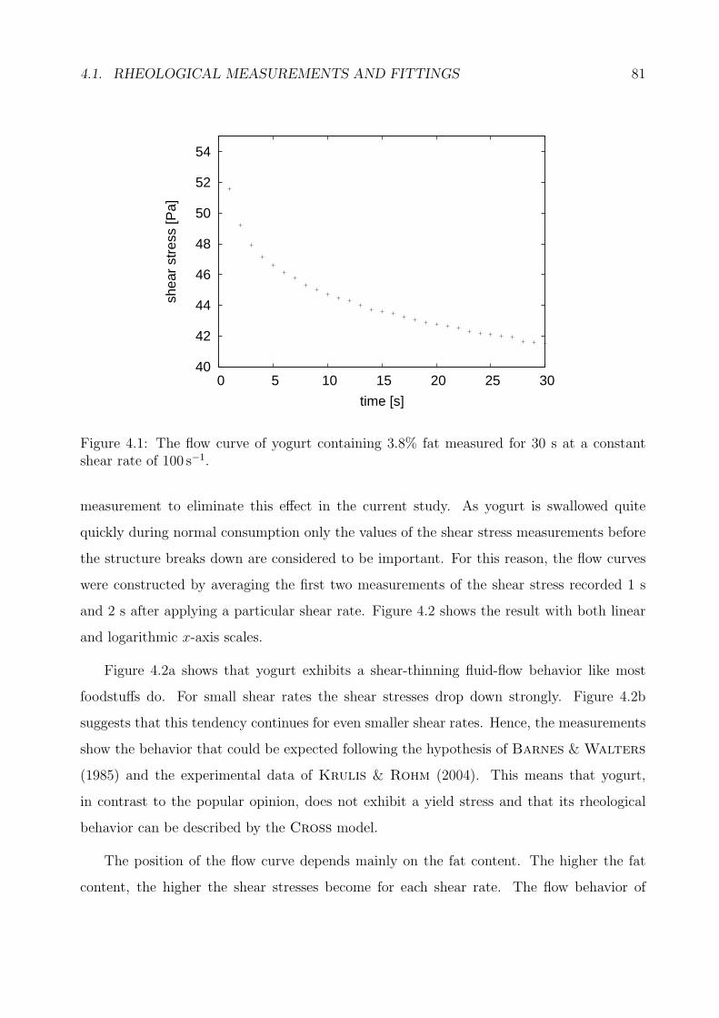
4.1. RHEOLOGICAL MEASUREMENTS AND FITTINGS 81
40
42
44
46
48
50
52
54
0 5 10 15 20 25 30
shea
r st
ress
[Pa]
time [s]
Figure 4.1: The flow curve of yogurt containing 3.8% fat measured for 30 s at a constantshear rate of 100 s−1.
measurement to eliminate this effect in the current study. As yogurt is swallowed quite
quickly during normal consumption only the values of the shear stress measurements before
the structure breaks down are considered to be important. For this reason, the flow curves
were constructed by averaging the first two measurements of the shear stress recorded 1 s
and 2 s after applying a particular shear rate. Figure 4.2 shows the result with both linear
and logarithmic x-axis scales.
Figure 4.2a shows that yogurt exhibits a shear-thinning fluid-flow behavior like most
foodstuffs do. For small shear rates the shear stresses drop down strongly. Figure 4.2b
suggests that this tendency continues for even smaller shear rates. Hence, the measurements
show the behavior that could be expected following the hypothesis of Barnes & Walters
(1985) and the experimental data of Krulis & Rohm (2004). This means that yogurt,
in contrast to the popular opinion, does not exhibit a yield stress and that its rheological
behavior can be described by the Cross model.
The position of the flow curve depends mainly on the fat content. The higher the fat
content, the higher the shear stresses become for each shear rate. The flow behavior of
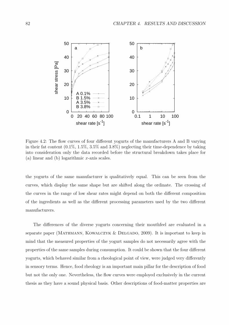
82 CHAPTER 4. RESULTS AND DISCUSSION
0
10
20
30
40
50
0 20 40 60 80 100
shea
r st
ress
[Pa]
shear rate [s-1]
a
A 0.1%B 1.5%A 3.5%B 3.8%
0
10
20
30
40
50
0.1 1 10 100
shear rate [s-1]
b
Figure 4.2: The flow curves of four different yogurts of the manufacturers A and B varyingin their fat content (0.1%, 1.5%, 3.5% and 3.8%) neglecting their time-dependence by takinginto consideration only the data recorded before the structural breakdown takes place for(a) linear and (b) logarithmic x-axis scales.
the yogurts of the same manufacturer is qualitatively equal. This can be seen from the
curves, which display the same shape but are shifted along the ordinate. The crossing of
the curves in the range of low shear rates might depend on both the different composition
of the ingredients as well as the different processing parameters used by the two different
manufacturers.
The differences of the diverse yogurts concerning their mouthfeel are evaluated in a
separate paper (Mathmann, Kowalczyk & Delgado, 2009). It is important to keep in
mind that the measured properties of the yogurt samples do not necessarily agree with the
properties of the same samples during consumption. It could be shown that the four different
yogurts, which behaved similar from a rheological point of view, were judged very differently
in sensory terms. Hence, food rheology is an important main pillar for the description of food
but not the only one. Nevertheless, the flow curves were employed exclusively in the current
thesis as they have a sound physical basis. Other descriptions of food-matter properties are
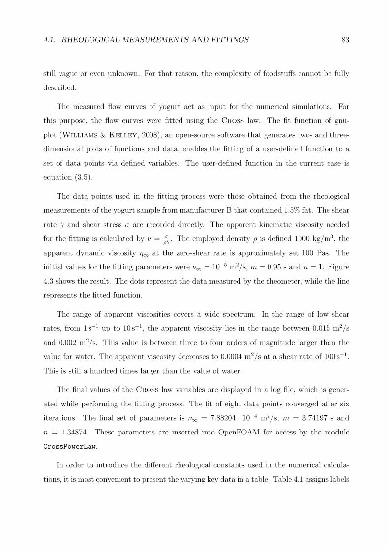
4.1. RHEOLOGICAL MEASUREMENTS AND FITTINGS 83
still vague or even unknown. For that reason, the complexity of foodstuffs cannot be fully
described.
The measured flow curves of yogurt act as input for the numerical simulations. For
this purpose, the flow curves were fitted using the Cross law. The fit function of gnu-
plot (Williams & Kelley, 2008), an open-source software that generates two- and three-
dimensional plots of functions and data, enables the fitting of a user-defined function to a
set of data points via defined variables. The user-defined function in the current case is
equation (3.5).
The data points used in the fitting process were those obtained from the rheological
measurements of the yogurt sample from manufacturer B that contained 1.5% fat. The shear
rate γ and shear stress σ are recorded directly. The apparent kinematic viscosity needed
for the fitting is calculated by ν = σργ. The employed density ρ is defined 1000 kg/m3, the
apparent dynamic viscosity η∞ at the zero-shear rate is approximately set 100 Pas. The
initial values for the fitting parameters were ν∞ = 10−5 m2/s, m = 0.95 s and n = 1. Figure
4.3 shows the result. The dots represent the data measured by the rheometer, while the line
represents the fitted function.
The range of apparent viscosities covers a wide spectrum. In the range of low shear
rates, from 1 s−1 up to 10 s−1, the apparent viscosity lies in the range between 0.015 m2/s
and 0.002 m2/s. This value is between three to four orders of magnitude larger than the
value for water. The apparent viscosity decreases to 0.0004 m2/s at a shear rate of 100 s−1.
This is still a hundred times larger than the value of water.
The final values of the Cross law variables are displayed in a log file, which is gener-
ated while performing the fitting process. The fit of eight data points converged after six
iterations. The final set of parameters is ν∞ = 7.88204 · 10−4 m2/s, m = 3.74197 s and
n = 1.34874. These parameters are inserted into OpenFOAM for access by the module
CrossPowerLaw.
In order to introduce the different rheological constants used in the numerical calcula-
tions, it is most convenient to present the varying key data in a table. Table 4.1 assigns labels
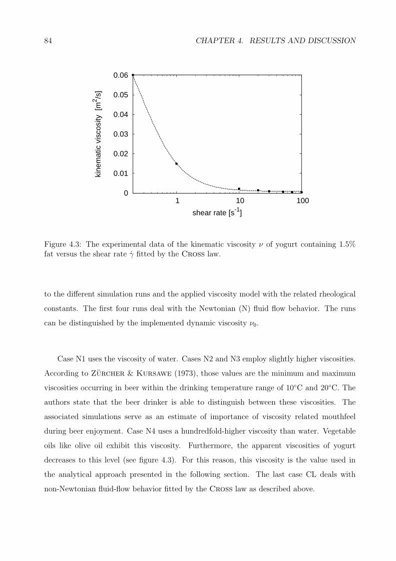
84 CHAPTER 4. RESULTS AND DISCUSSION
0
0.01
0.02
0.03
0.04
0.05
0.06
1 10 100
kine
mat
ic v
isco
sity
[m
2 /s]
shear rate [s-1]
Figure 4.3: The experimental data of the kinematic viscosity ν of yogurt containing 1.5%fat versus the shear rate γ fitted by the Cross law.
to the different simulation runs and the applied viscosity model with the related rheological
constants. The first four runs deal with the Newtonian (N) fluid flow behavior. The runs
can be distinguished by the implemented dynamic viscosity ν0.
Case N1 uses the viscosity of water. Cases N2 and N3 employ slightly higher viscosities.
According to Zurcher & Kursawe (1973), those values are the minimum and maximum
viscosities occurring in beer within the drinking temperature range of 10◦C and 20◦C. The
authors state that the beer drinker is able to distinguish between these viscosities. The
associated simulations serve as an estimate of importance of viscosity related mouthfeel
during beer enjoyment. Case N4 uses a hundredfold-higher viscosity than water. Vegetable
oils like olive oil exhibit this viscosity. Furthermore, the apparent viscosities of yogurt
decreases to this level (see figure 4.3). For this reason, this viscosity is the value used in
the analytical approach presented in the following section. The last case CL deals with
non-Newtonian fluid-flow behavior fitted by the Cross law as described above.
4.2. THEORY OF LUBRICATION 85
4.2 Theory of Lubrication
The results of the theory of lubrication are subdivided into the four different approaches of
squeezing flow introduced and derived in sections 3.3.3 to 3.3.6. As the fluid flow takes place
in the sagittal plane of the oral cavity the focus is mainly on the key points in this plane.
4.2.1 Plane Circular Parallel Plates - Stefan Equation
The Stefan equation (3.30) gives a parabolic profile for the pressure distribution p−p0 along
the radial coordinate r. Inserting the dynamic viscosity η = 100 mPas, which lies in the order
of magnitude of vegetable oils like olive oil and the apparent viscosity of yogurt presented in
the previous section, the uniform plate velocity vp = 1 cm/s determined in section 3.4.5, the
minimum film thickness h0 = 1 mm and the plate radius Rp2 = 29 mm yields the pressure
distribution illustrated in figure 4.4. The maximum pressure difference p− p0 in the center
of the plates for this configuration is 2523 Pa.
In order to present the impact of the different radii that can be found in table 3.2,
figure 4.5 depicts the maximum pressures occurring in the center of the plates depending on
their radius. The Stefan equation (3.30) simplifies to
pmax − p0 = 3ηvph30
R2 (4.1)
for this purpose. The values inserted for the dynamic viscosity η, the uniform plate velocity vp
and the minimum film thickness h0 remain the same.
The maximum pressure goes from 972 Pa to 3675 Pa for the plate radius varying between
18 mm and 35 mm. Over this range of realistic dimensions for the oral cavity, a huge pressure
difference of 2703 Pa is encountered.
The velocity components are evaluated together in terms of the magnitude of velocity.
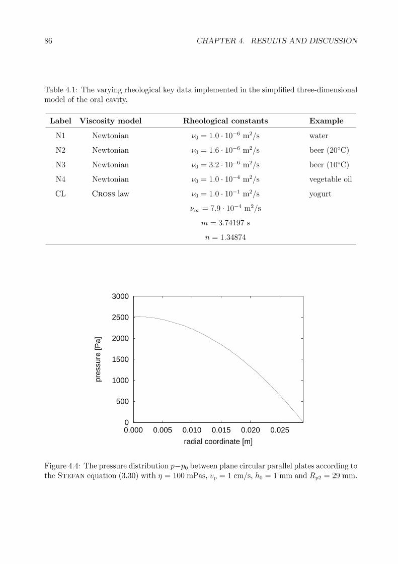
86 CHAPTER 4. RESULTS AND DISCUSSION
Table 4.1: The varying rheological key data implemented in the simplified three-dimensionalmodel of the oral cavity.
Label Viscosity model Rheological constants Example
N1 Newtonian ν0 = 1.0 · 10−6 m2/s water
N2 Newtonian ν0 = 1.6 · 10−6 m2/s beer (20◦C)
N3 Newtonian ν0 = 3.2 · 10−6 m2/s beer (10◦C)
N4 Newtonian ν0 = 1.0 · 10−4 m2/s vegetable oil
CL Cross law ν0 = 1.0 · 10−1 m2/s yogurt
ν∞ = 7.9 · 10−4 m2/s
m = 3.74197 s
n = 1.34874
0
500
1000
1500
2000
2500
3000
0.000 0.005 0.010 0.015 0.020 0.025
pres
sure
[Pa]
radial coordinate [m]
Figure 4.4: The pressure distribution p−p0 between plane circular parallel plates according tothe Stefan equation (3.30) with η = 100 mPas, vp = 1 cm/s, h0 = 1 mm and Rp2 = 29 mm.
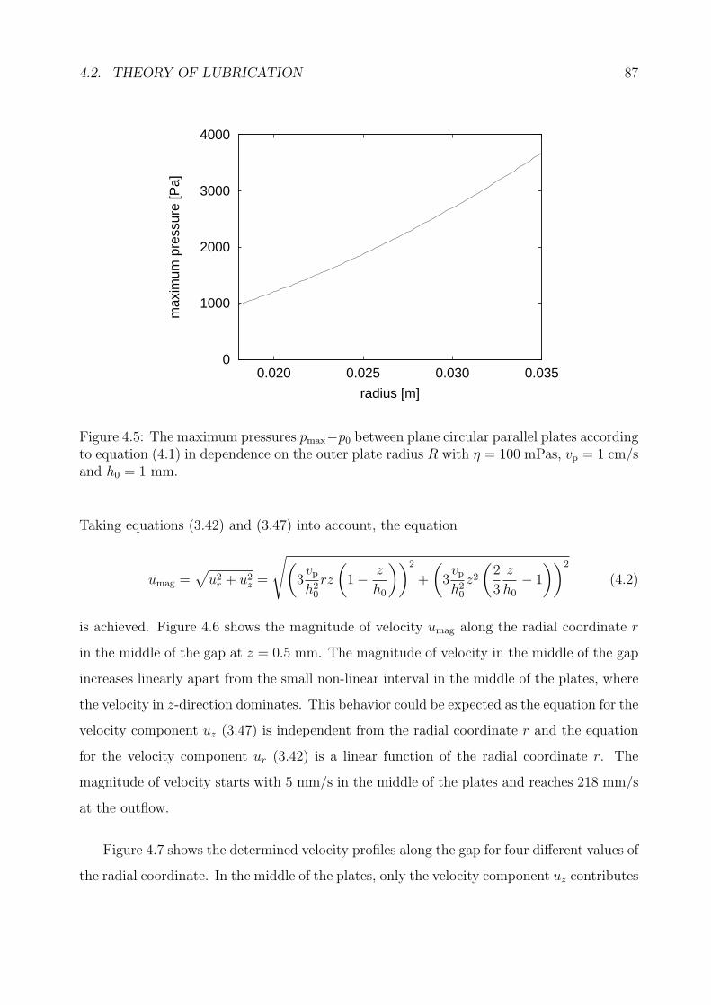
4.2. THEORY OF LUBRICATION 87
0
1000
2000
3000
4000
0.020 0.025 0.030 0.035
max
imum
pre
ssur
e [P
a]
radius [m]
Figure 4.5: The maximum pressures pmax−p0 between plane circular parallel plates accordingto equation (4.1) in dependence on the outer plate radius R with η = 100 mPas, vp = 1 cm/sand h0 = 1 mm.
Taking equations (3.42) and (3.47) into account, the equation
umag =√u2r + u2z =
√(3vph20rz
(1− z
h0
))2
+
(3vph20z2(2
3
z
h0− 1
))2
(4.2)
is achieved. Figure 4.6 shows the magnitude of velocity umag along the radial coordinate r
in the middle of the gap at z = 0.5 mm. The magnitude of velocity in the middle of the gap
increases linearly apart from the small non-linear interval in the middle of the plates, where
the velocity in z-direction dominates. This behavior could be expected as the equation for the
velocity component uz (3.47) is independent from the radial coordinate r and the equation
for the velocity component ur (3.42) is a linear function of the radial coordinate r. The
magnitude of velocity starts with 5 mm/s in the middle of the plates and reaches 218 mm/s
at the outflow.
Figure 4.7 shows the determined velocity profiles along the gap for four different values of
the radial coordinate. In the middle of the plates, only the velocity component uz contributes
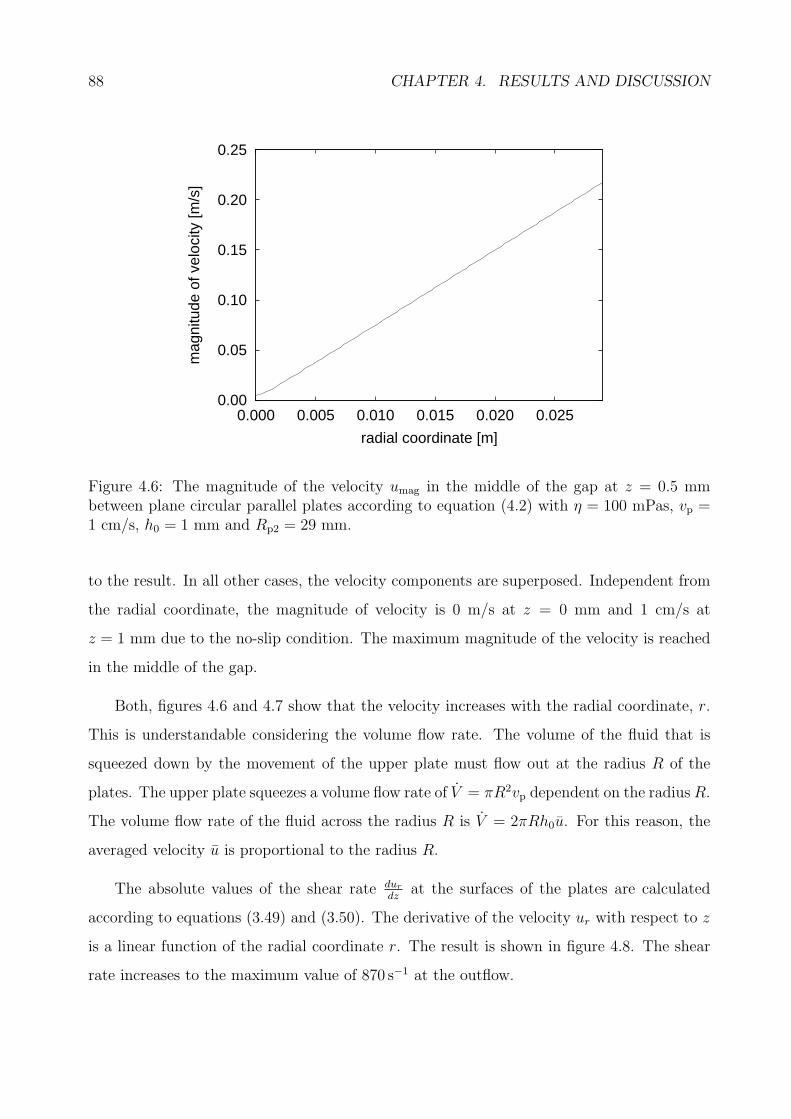
88 CHAPTER 4. RESULTS AND DISCUSSION
0.00
0.05
0.10
0.15
0.20
0.25
0.000 0.005 0.010 0.015 0.020 0.025
mag
nitu
de o
f vel
ocity
[m/s
]
radial coordinate [m]
Figure 4.6: The magnitude of the velocity umag in the middle of the gap at z = 0.5 mmbetween plane circular parallel plates according to equation (4.2) with η = 100 mPas, vp =1 cm/s, h0 = 1 mm and Rp2 = 29 mm.
to the result. In all other cases, the velocity components are superposed. Independent from
the radial coordinate, the magnitude of velocity is 0 m/s at z = 0 mm and 1 cm/s at
z = 1 mm due to the no-slip condition. The maximum magnitude of the velocity is reached
in the middle of the gap.
Both, figures 4.6 and 4.7 show that the velocity increases with the radial coordinate, r.
This is understandable considering the volume flow rate. The volume of the fluid that is
squeezed down by the movement of the upper plate must flow out at the radius R of the
plates. The upper plate squeezes a volume flow rate of V = πR2vp dependent on the radius R.
The volume flow rate of the fluid across the radius R is V = 2πRh0u. For this reason, the
averaged velocity u is proportional to the radius R.
The absolute values of the shear rate dur
dzat the surfaces of the plates are calculated
according to equations (3.49) and (3.50). The derivative of the velocity ur with respect to z
is a linear function of the radial coordinate r. The result is shown in figure 4.8. The shear
rate increases to the maximum value of 870 s−1 at the outflow.
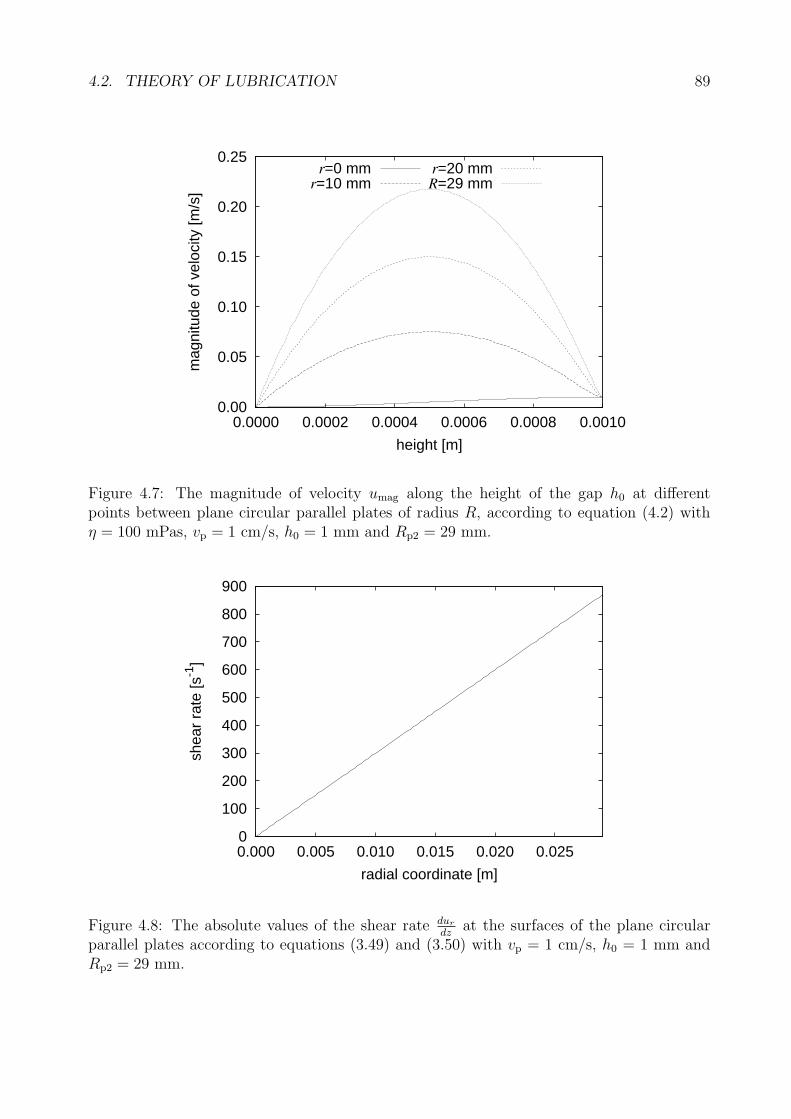
4.2. THEORY OF LUBRICATION 89
0.00
0.05
0.10
0.15
0.20
0.25
0.0000 0.0002 0.0004 0.0006 0.0008 0.0010
mag
nitu
de o
f vel
ocity
[m/s
]
height [m]
r=0 mmr=10 mm
r=20 mmR=29 mm
Figure 4.7: The magnitude of velocity umag along the height of the gap h0 at differentpoints between plane circular parallel plates of radius R, according to equation (4.2) withη = 100 mPas, vp = 1 cm/s, h0 = 1 mm and Rp2 = 29 mm.
0
100
200
300
400
500
600
700
800
900
0.000 0.005 0.010 0.015 0.020 0.025
shea
r ra
te [s
-1]
radial coordinate [m]
Figure 4.8: The absolute values of the shear rate dur
dzat the surfaces of the plane circular
parallel plates according to equations (3.49) and (3.50) with vp = 1 cm/s, h0 = 1 mm andRp2 = 29 mm.
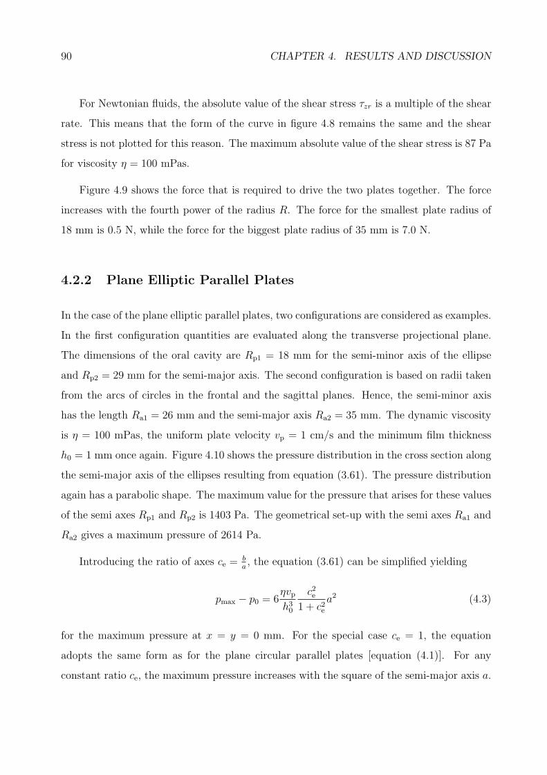
90 CHAPTER 4. RESULTS AND DISCUSSION
For Newtonian fluids, the absolute value of the shear stress τzr is a multiple of the shear
rate. This means that the form of the curve in figure 4.8 remains the same and the shear
stress is not plotted for this reason. The maximum absolute value of the shear stress is 87 Pa
for viscosity η = 100 mPas.
Figure 4.9 shows the force that is required to drive the two plates together. The force
increases with the fourth power of the radius R. The force for the smallest plate radius of
18 mm is 0.5 N, while the force for the biggest plate radius of 35 mm is 7.0 N.
4.2.2 Plane Elliptic Parallel Plates
In the case of the plane elliptic parallel plates, two configurations are considered as examples.
In the first configuration quantities are evaluated along the transverse projectional plane.
The dimensions of the oral cavity are Rp1 = 18 mm for the semi-minor axis of the ellipse
and Rp2 = 29 mm for the semi-major axis. The second configuration is based on radii taken
from the arcs of circles in the frontal and the sagittal planes. Hence, the semi-minor axis
has the length Ra1 = 26 mm and the semi-major axis Ra2 = 35 mm. The dynamic viscosity
is η = 100 mPas, the uniform plate velocity vp = 1 cm/s and the minimum film thickness
h0 = 1 mm once again. Figure 4.10 shows the pressure distribution in the cross section along
the semi-major axis of the ellipses resulting from equation (3.61). The pressure distribution
again has a parabolic shape. The maximum value for the pressure that arises for these values
of the semi axes Rp1 and Rp2 is 1403 Pa. The geometrical set-up with the semi axes Ra1 and
Ra2 gives a maximum pressure of 2614 Pa.
Introducing the ratio of axes ce =ba, the equation (3.61) can be simplified yielding
pmax − p0 = 6ηvph30
c2e1 + c2e
a2 (4.3)
for the maximum pressure at x = y = 0 mm. For the special case ce = 1, the equation
adopts the same form as for the plane circular parallel plates [equation (4.1)]. For any
constant ratio ce, the maximum pressure increases with the square of the semi-major axis a.
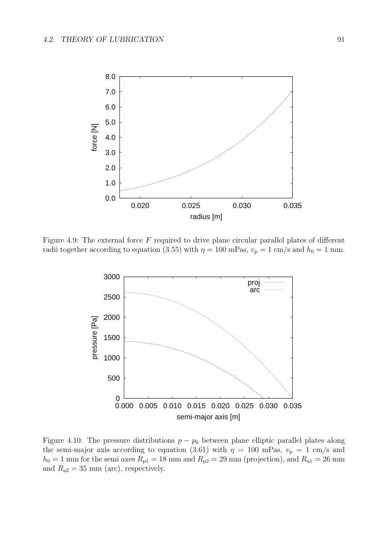
4.2. THEORY OF LUBRICATION 91
0.0
1.0
2.0
3.0
4.0
5.0
6.0
7.0
8.0
0.020 0.025 0.030 0.035
forc
e [N
]
radius [m]
Figure 4.9: The external force F required to drive plane circular parallel plates of differentradii together according to equation (3.55) with η = 100 mPas, vp = 1 cm/s and h0 = 1 mm.
0
500
1000
1500
2000
2500
3000
0.000 0.005 0.010 0.015 0.020 0.025 0.030 0.035
pres
sure
[Pa]
semi-major axis [m]
projarc
Figure 4.10: The pressure distributions p − p0 between plane elliptic parallel plates alongthe semi-major axis according to equation (3.61) with η = 100 mPas, vp = 1 cm/s andh0 = 1 mm for the semi axes Rp1 = 18 mm and Rp2 = 29 mm (projection), and Ra1 = 26 mmand Ra2 = 35 mm (arc), respectively.

92 CHAPTER 4. RESULTS AND DISCUSSION
In the present study, the ratio of the axes is not the same for the arc and projection
configurations. It is 0.62 for the projection configuration and 0.74 for the arc configuration.
In order to demonstrate the influence of altering ratios ce, figure 4.11 shows the maximum
pressure distribution for both semi-major axes. Concerning the semi-major axis Rp2, the
pressure increases from 1401 Pa for the ratio ce = 0.62 to 2523 Pa for the ratio ce = 1
representing the system of plane circular parallel plates. The pressures arising according
to the semi-major axis Ra2 are 2041 Pa and 3675 Pa. This means that the maximum
occurring pressure of the elliptic configuration is 44% smaller compared to the circular one
for a minimum ratio ce = 0.62. For this reason, the shape of plates is of vital importance in
the plane configuration.
A comparison between plane circular and elliptic plates using equal plate areas can also
be performed. The corresponding radii of the circles can be calculated by r =√ab yielding
23 mm and 30 mm for the configurations discussed above. The corresponding maximum
pressures can be calculated as being 1566 Pa and 2730 Pa (figure 4.5). Considering the same
areas for both shows that the maximum pressures are smaller for ellipses than for circles. In
the case of the projection configuration, the difference is about 10%; in the case of the arc
configuration, it is only 4%. Keeping in mind the ratio of the axes, it can again be stated
that the difference diminishes the more the ratio ce converges to 1. Nevertheless, the elliptic
shape of the oral cavity suggests that the result of the Stefan equation (3.30) should be
corrected by an factor of up to 10%.
Figure 4.12 shows the magnitudes of the velocity in the main fluid-flow direction along
the ellipse axes. In analogy to equation (4.2), the underlying equation equals the square
root of the sum of the squares of the velocity components in the x- and z-directions as well
as the y- and z-directions [equations (3.47), (3.69) and (3.70)]. The resulting magnitudes of
velocity are again linear along the axis apart from the small interval at the middle of the
plates where the velocity component in the z-direction dominates. They are bigger along
the minor axes than along the major axes. This can be expected from equations (3.69) and
(3.70).
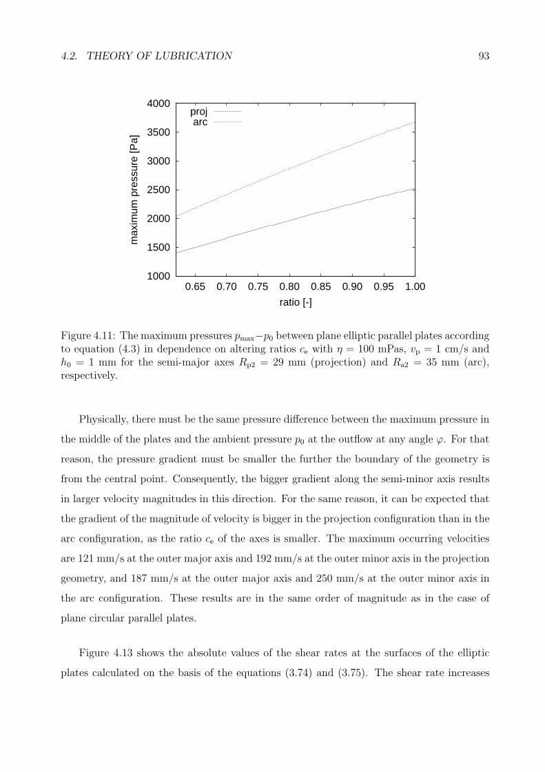
4.2. THEORY OF LUBRICATION 93
1000
1500
2000
2500
3000
3500
4000
0.65 0.70 0.75 0.80 0.85 0.90 0.95 1.00
max
imum
pre
ssur
e [P
a]
ratio [-]
projarc
Figure 4.11: The maximum pressures pmax−p0 between plane elliptic parallel plates accordingto equation (4.3) in dependence on altering ratios ce with η = 100 mPas, vp = 1 cm/s andh0 = 1 mm for the semi-major axes Rp2 = 29 mm (projection) and Ra2 = 35 mm (arc),respectively.
Physically, there must be the same pressure difference between the maximum pressure in
the middle of the plates and the ambient pressure p0 at the outflow at any angle φ. For that
reason, the pressure gradient must be smaller the further the boundary of the geometry is
from the central point. Consequently, the bigger gradient along the semi-minor axis results
in larger velocity magnitudes in this direction. For the same reason, it can be expected that
the gradient of the magnitude of velocity is bigger in the projection configuration than in the
arc configuration, as the ratio ce of the axes is smaller. The maximum occurring velocities
are 121 mm/s at the outer major axis and 192 mm/s at the outer minor axis in the projection
geometry, and 187 mm/s at the outer major axis and 250 mm/s at the outer minor axis in
the arc configuration. These results are in the same order of magnitude as in the case of
plane circular parallel plates.
Figure 4.13 shows the absolute values of the shear rates at the surfaces of the elliptic
plates calculated on the basis of the equations (3.74) and (3.75). The shear rate increases
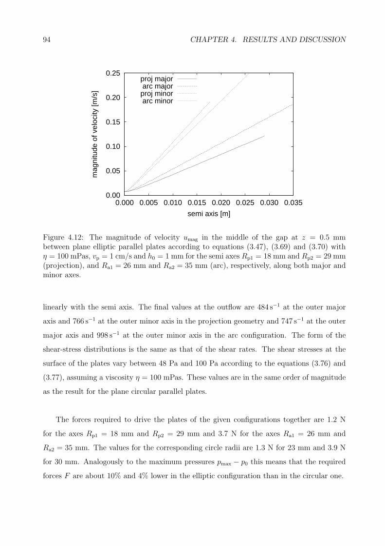
94 CHAPTER 4. RESULTS AND DISCUSSION
0.00
0.05
0.10
0.15
0.20
0.25
0.000 0.005 0.010 0.015 0.020 0.025 0.030 0.035
mag
nitu
de o
f vel
ocity
[m/s
]
semi axis [m]
proj majorarc majorproj minorarc minor
Figure 4.12: The magnitude of velocity umag in the middle of the gap at z = 0.5 mmbetween plane elliptic parallel plates according to equations (3.47), (3.69) and (3.70) withη = 100 mPas, vp = 1 cm/s and h0 = 1 mm for the semi axes Rp1 = 18 mm and Rp2 = 29 mm(projection), and Ra1 = 26 mm and Ra2 = 35 mm (arc), respectively, along both major andminor axes.
linearly with the semi axis. The final values at the outflow are 484 s−1 at the outer major
axis and 766 s−1 at the outer minor axis in the projection geometry and 747 s−1 at the outer
major axis and 998 s−1 at the outer minor axis in the arc configuration. The form of the
shear-stress distributions is the same as that of the shear rates. The shear stresses at the
surface of the plates vary between 48 Pa and 100 Pa according to the equations (3.76) and
(3.77), assuming a viscosity η = 100 mPas. These values are in the same order of magnitude
as the result for the plane circular parallel plates.
The forces required to drive the plates of the given configurations together are 1.2 N
for the axes Rp1 = 18 mm and Rp2 = 29 mm and 3.7 N for the axes Ra1 = 26 mm and
Ra2 = 35 mm. The values for the corresponding circle radii are 1.3 N for 23 mm and 3.9 N
for 30 mm. Analogously to the maximum pressures pmax − p0 this means that the required
forces F are about 10% and 4% lower in the elliptic configuration than in the circular one.
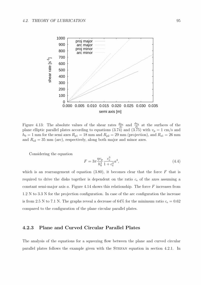
4.2. THEORY OF LUBRICATION 95
0
100
200
300
400
500
600
700
800
900
1000
0.000 0.005 0.010 0.015 0.020 0.025 0.030 0.035
shea
r ra
te [s
-1]
semi axis [m]
proj majorarc major
proj minorarc minor
Figure 4.13: The absolute values of the shear rates dux
dzand duy
dzat the surfaces of the
plane elliptic parallel plates according to equations (3.74) and (3.75) with vp = 1 cm/s andh0 = 1 mm for the semi axes Rp1 = 18 mm and Rp2 = 29 mm (projection), and Ra1 = 26 mmand Ra2 = 35 mm (arc), respectively, along both major and minor axes.
Considering the equation
F = 3πηvph30
c3e1 + c2e
a4, (4.4)
which is an rearrangement of equation (3.80), it becomes clear that the force F that is
required to drive the disks together is dependent on the ratio ce of the axes assuming a
constant semi-major axis a. Figure 4.14 shows this relationship. The force F increases from
1.2 N to 3.3 N for the projection configuration. In case of the arc configuration the increase
is from 2.5 N to 7.1 N. The graphs reveal a decrease of 64% for the minimum ratio ce = 0.62
compared to the configuration of the plane circular parallel plates.
4.2.3 Plane and Curved Circular Parallel Plates
The analysis of the equations for a squeezing flow between the plane and curved circular
parallel plates follows the example given with the Stefan equation in section 4.2.1. In
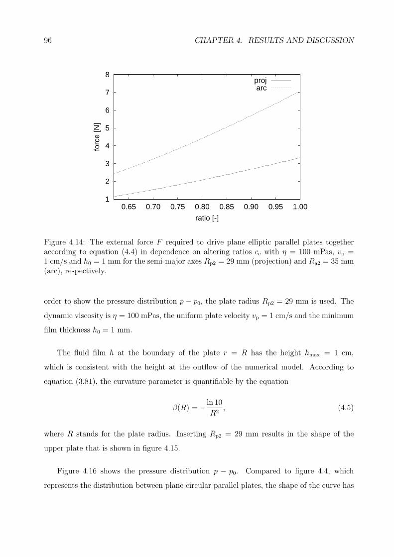
96 CHAPTER 4. RESULTS AND DISCUSSION
1
2
3
4
5
6
7
8
0.65 0.70 0.75 0.80 0.85 0.90 0.95 1.00
forc
e [N
]
ratio [-]
projarc
Figure 4.14: The external force F required to drive plane elliptic parallel plates togetheraccording to equation (4.4) in dependence on altering ratios ce with η = 100 mPas, vp =1 cm/s and h0 = 1 mm for the semi-major axes Rp2 = 29 mm (projection) and Ra2 = 35 mm(arc), respectively.
order to show the pressure distribution p − p0, the plate radius Rp2 = 29 mm is used. The
dynamic viscosity is η = 100 mPas, the uniform plate velocity vp = 1 cm/s and the minimum
film thickness h0 = 1 mm.
The fluid film h at the boundary of the plate r = R has the height hmax = 1 cm,
which is consistent with the height at the outflow of the numerical model. According to
equation (3.81), the curvature parameter is quantifiable by the equation
β(R) = − ln 10
R2, (4.5)
where R stands for the plate radius. Inserting Rp2 = 29 mm results in the shape of the
upper plate that is shown in figure 4.15.
Figure 4.16 shows the pressure distribution p − p0. Compared to figure 4.4, which
represents the distribution between plane circular parallel plates, the shape of the curve has
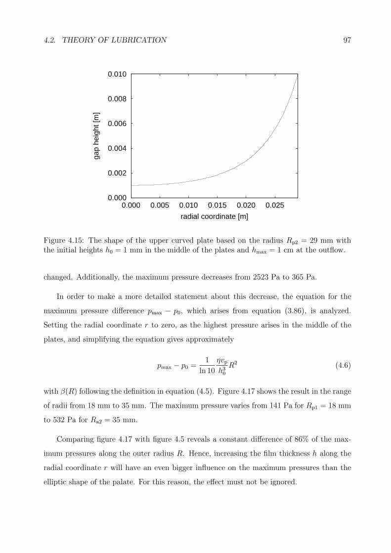
4.2. THEORY OF LUBRICATION 97
0.000
0.002
0.004
0.006
0.008
0.010
0.000 0.005 0.010 0.015 0.020 0.025
gap
heig
ht [m
]
radial coordinate [m]
Figure 4.15: The shape of the upper curved plate based on the radius Rp2 = 29 mm withthe initial heights h0 = 1 mm in the middle of the plates and hmax = 1 cm at the outflow.
changed. Additionally, the maximum pressure decreases from 2523 Pa to 365 Pa.
In order to make a more detailed statement about this decrease, the equation for the
maximum pressure difference pmax − p0, which arises from equation (3.86), is analyzed.
Setting the radial coordinate r to zero, as the highest pressure arises in the middle of the
plates, and simplifying the equation gives approximately
pmax − p0 =1
ln 10
ηvph30
R2 (4.6)
with β(R) following the definition in equation (4.5). Figure 4.17 shows the result in the range
of radii from 18 mm to 35 mm. The maximum pressure varies from 141 Pa for Rp1 = 18 mm
to 532 Pa for Ra2 = 35 mm.
Comparing figure 4.17 with figure 4.5 reveals a constant difference of 86% of the max-
imum pressures along the outer radius R. Hence, increasing the film thickness h along the
radial coordinate r will have an even bigger influence on the maximum pressures than the
elliptic shape of the palate. For this reason, the effect must not be ignored.

98 CHAPTER 4. RESULTS AND DISCUSSION
0
50
100
150
200
250
300
350
400
0.000 0.005 0.010 0.015 0.020 0.025
pres
sure
[Pa]
radial coordinate [m]
Figure 4.16: The pressure distribution p−p0 between plane and curved circular parallel platesaccording to equation (3.86) with η = 100 mPas, vp = 1 cm/s, h0 = 1 mm, hmax = 1 cm andRp2 = 29 mm.
0
100
200
300
400
500
600
0.020 0.025 0.030 0.035
max
imum
pre
ssur
e [P
a]
radius [m]
Figure 4.17: The maximum pressures pmax − p0 between plane and curved circular par-allel plates as a function of the outer plate radius R according to equation (4.6) withη = 100 mPas, vp = 1 cm/s, h0 = 1 mm and the respective height hmax = 1 cm at theboundary of the plate.

4.2. THEORY OF LUBRICATION 99
Figure 4.18 shows the velocity distribution in the r-direction based on equation (3.92).
The velocity at the outlet is 22 mm/s. In contrast to the previous calculations, the maximum
velocity is not reached at the outlet. The maximum value of 61.5 mm/s can be found at
r = 13.5 mm. From there on the height of the gap increases significantly and the pressure
drops down. As the velocity distribution along the radial coordinate is quite different from
the previous cases, a direct comparison is not possible. It can only be stated that the
maximum occurring velocities drop to about a quarter of that compared with the geometry
of two plane circular parallel plates. Figure 4.19 shows the velocity profiles in the gap for
four different values of the radial coordinate r. The profiles are symmetric. The maximum
values follow the distribution shown in figure 4.18.
Figure 4.20 shows the absolute values of the shear rate at the surfaces of the plates
according to equation (3.94). The shear rate has its highest value dudz
= 174 s−1 at r = 9.6 mm.
This is only one fifth of the shear rate occurring at the outflow of the plane circular parallel
plates. The maximum value of the occurring shear stress in a Newtonian medium with a
viscosity η = 100 mPas is 17.4 Pa.
Figure 4.21 shows the force that is required to drive the plates together in dependence
on different values of the plate radius R in the range from 18 mm to 35 mm. The forces
range from 21 mN to 296 mN. Compared to the plane circular parallel plates the required
force is 96% smaller.
4.2.4 Sphere in a Hemisphere
The calculation of a sphere in a hemisphere by means of equation (3.106) is based on the
rounded-down radius through the key points in the sagittal plane R2 = 34 mm, which is
employed for the hemisphere. The minimum distance between the sphere and hemisphere
in the z-direction adopts the same value occurring in the model of the numerical simulation,
namely h0 = 1 mm. This distance is normally maintained in the front part of the numerical
model.
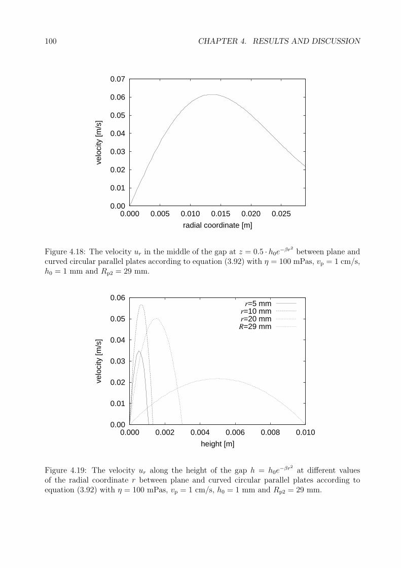
100 CHAPTER 4. RESULTS AND DISCUSSION
0.00
0.01
0.02
0.03
0.04
0.05
0.06
0.07
0.000 0.005 0.010 0.015 0.020 0.025
velo
city
[m/s
]
radial coordinate [m]
Figure 4.18: The velocity ur in the middle of the gap at z = 0.5 · h0e−βr2 between plane andcurved circular parallel plates according to equation (3.92) with η = 100 mPas, vp = 1 cm/s,h0 = 1 mm and Rp2 = 29 mm.
0.00
0.01
0.02
0.03
0.04
0.05
0.06
0.000 0.002 0.004 0.006 0.008 0.010
velo
city
[m/s
]
height [m]
r=5 mmr=10 mmr=20 mmR=29 mm
Figure 4.19: The velocity ur along the height of the gap h = h0e−βr2 at different values
of the radial coordinate r between plane and curved circular parallel plates according toequation (3.92) with η = 100 mPas, vp = 1 cm/s, h0 = 1 mm and Rp2 = 29 mm.
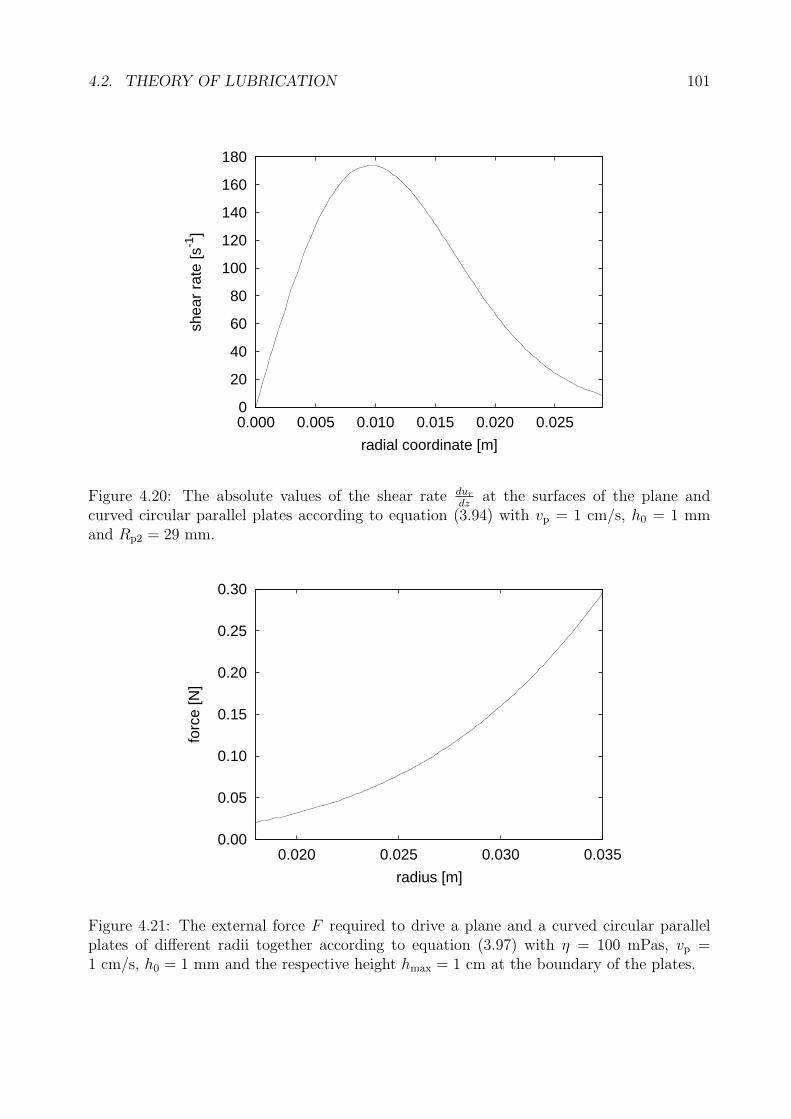
4.2. THEORY OF LUBRICATION 101
0
20
40
60
80
100
120
140
160
180
0.000 0.005 0.010 0.015 0.020 0.025
shea
r ra
te [s
-1]
radial coordinate [m]
Figure 4.20: The absolute values of the shear rate dur
dzat the surfaces of the plane and
curved circular parallel plates according to equation (3.94) with vp = 1 cm/s, h0 = 1 mmand Rp2 = 29 mm.
0.00
0.05
0.10
0.15
0.20
0.25
0.30
0.020 0.025 0.030 0.035
forc
e [N
]
radius [m]
Figure 4.21: The external force F required to drive a plane and a curved circular parallelplates of different radii together according to equation (3.97) with η = 100 mPas, vp =1 cm/s, h0 = 1 mm and the respective height hmax = 1 cm at the boundary of the plates.
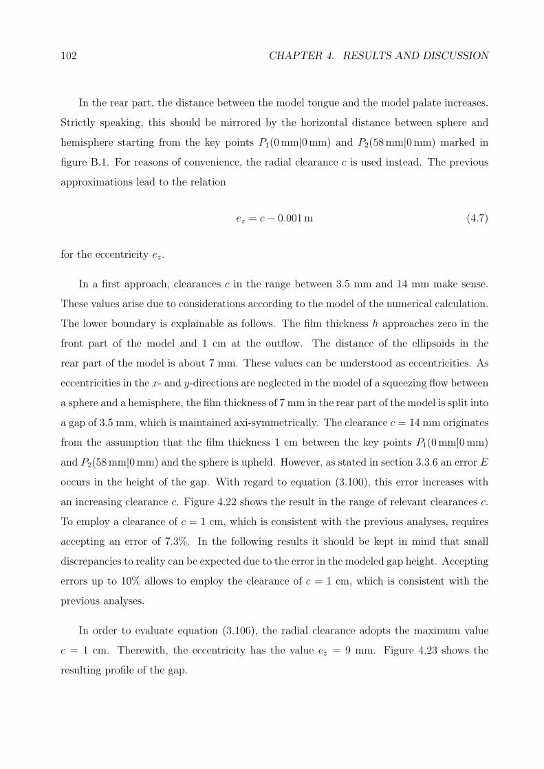
102 CHAPTER 4. RESULTS AND DISCUSSION
In the rear part, the distance between the model tongue and the model palate increases.
Strictly speaking, this should be mirrored by the horizontal distance between sphere and
hemisphere starting from the key points P1(0mm|0mm) and P2(58mm|0mm) marked in
figure B.1. For reasons of convenience, the radial clearance c is used instead. The previous
approximations lead to the relation
ez = c− 0.001m (4.7)
for the eccentricity ez.
In a first approach, clearances c in the range between 3.5 mm and 14 mm make sense.
These values arise due to considerations according to the model of the numerical calculation.
The lower boundary is explainable as follows. The film thickness h approaches zero in the
front part of the model and 1 cm at the outflow. The distance of the ellipsoids in the
rear part of the model is about 7 mm. These values can be understood as eccentricities. As
eccentricities in the x- and y-directions are neglected in the model of a squeezing flow between
a sphere and a hemisphere, the film thickness of 7 mm in the rear part of the model is split into
a gap of 3.5 mm, which is maintained axi-symmetrically. The clearance c = 14 mm originates
from the assumption that the film thickness 1 cm between the key points P1(0mm|0mm)
and P2(58mm|0mm) and the sphere is upheld. However, as stated in section 3.3.6 an error E
occurs in the height of the gap. With regard to equation (3.100), this error increases with
an increasing clearance c. Figure 4.22 shows the result in the range of relevant clearances c.
To employ a clearance of c = 1 cm, which is consistent with the previous analyses, requires
accepting an error of 7.3%. In the following results it should be kept in mind that small
discrepancies to reality can be expected due to the error in the modeled gap height. Accepting
errors up to 10% allows to employ the clearance of c = 1 cm, which is consistent with the
previous analyses.
In order to evaluate equation (3.106), the radial clearance adopts the maximum value
c = 1 cm. Therewith, the eccentricity has the value ez = 9 mm. Figure 4.23 shows the
resulting profile of the gap.
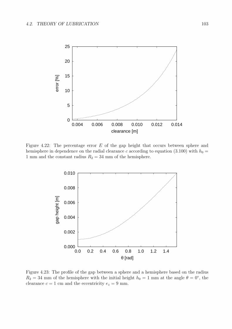
4.2. THEORY OF LUBRICATION 103
0
5
10
15
20
25
0.004 0.006 0.008 0.010 0.012 0.014
erro
r [%
]
clearance [m]
Figure 4.22: The percentage error E of the gap height that occurs between sphere andhemisphere in dependence on the radial clearance c according to equation (3.100) with h0 =1 mm and the constant radius R2 = 34 mm of the hemisphere.
0.000
0.002
0.004
0.006
0.008
0.010
0.0 0.2 0.4 0.6 0.8 1.0 1.2 1.4
gap
heig
ht [m
]
θ [rad]
Figure 4.23: The profile of the gap between a sphere and a hemisphere based on the radiusR2 = 34 mm of the hemisphere with the initial height h0 = 1 mm at the angle θ = 0◦, theclearance c = 1 cm and the eccentricity ez = 9 mm.
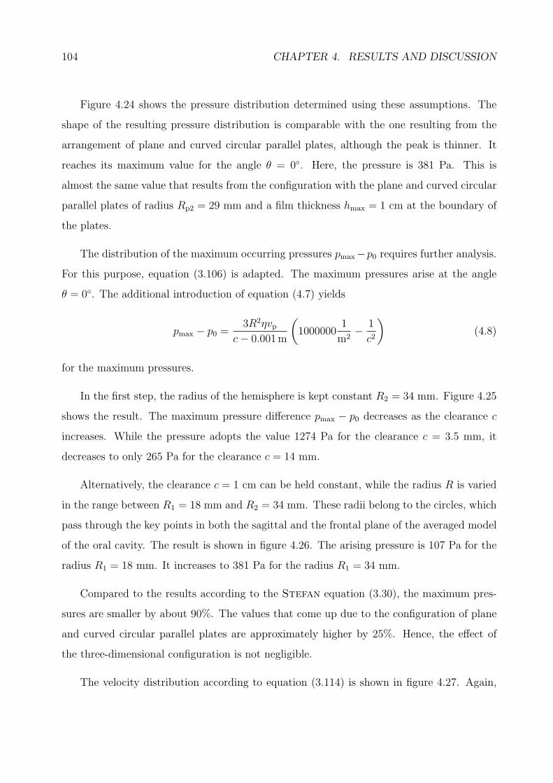
104 CHAPTER 4. RESULTS AND DISCUSSION
Figure 4.24 shows the pressure distribution determined using these assumptions. The
shape of the resulting pressure distribution is comparable with the one resulting from the
arrangement of plane and curved circular parallel plates, although the peak is thinner. It
reaches its maximum value for the angle θ = 0◦. Here, the pressure is 381 Pa. This is
almost the same value that results from the configuration with the plane and curved circular
parallel plates of radius Rp2 = 29 mm and a film thickness hmax = 1 cm at the boundary of
the plates.
The distribution of the maximum occurring pressures pmax−p0 requires further analysis.
For this purpose, equation (3.106) is adapted. The maximum pressures arise at the angle
θ = 0◦. The additional introduction of equation (4.7) yields
pmax − p0 =3R2ηvp
c− 0.001m
(1000000
1
m2− 1
c2
)(4.8)
for the maximum pressures.
In the first step, the radius of the hemisphere is kept constant R2 = 34 mm. Figure 4.25
shows the result. The maximum pressure difference pmax − p0 decreases as the clearance c
increases. While the pressure adopts the value 1274 Pa for the clearance c = 3.5 mm, it
decreases to only 265 Pa for the clearance c = 14 mm.
Alternatively, the clearance c = 1 cm can be held constant, while the radius R is varied
in the range between R1 = 18 mm and R2 = 34 mm. These radii belong to the circles, which
pass through the key points in both the sagittal and the frontal plane of the averaged model
of the oral cavity. The result is shown in figure 4.26. The arising pressure is 107 Pa for the
radius R1 = 18 mm. It increases to 381 Pa for the radius R1 = 34 mm.
Compared to the results according to the Stefan equation (3.30), the maximum pres-
sures are smaller by about 90%. The values that come up due to the configuration of plane
and curved circular parallel plates are approximately higher by 25%. Hence, the effect of
the three-dimensional configuration is not negligible.
The velocity distribution according to equation (3.114) is shown in figure 4.27. Again,
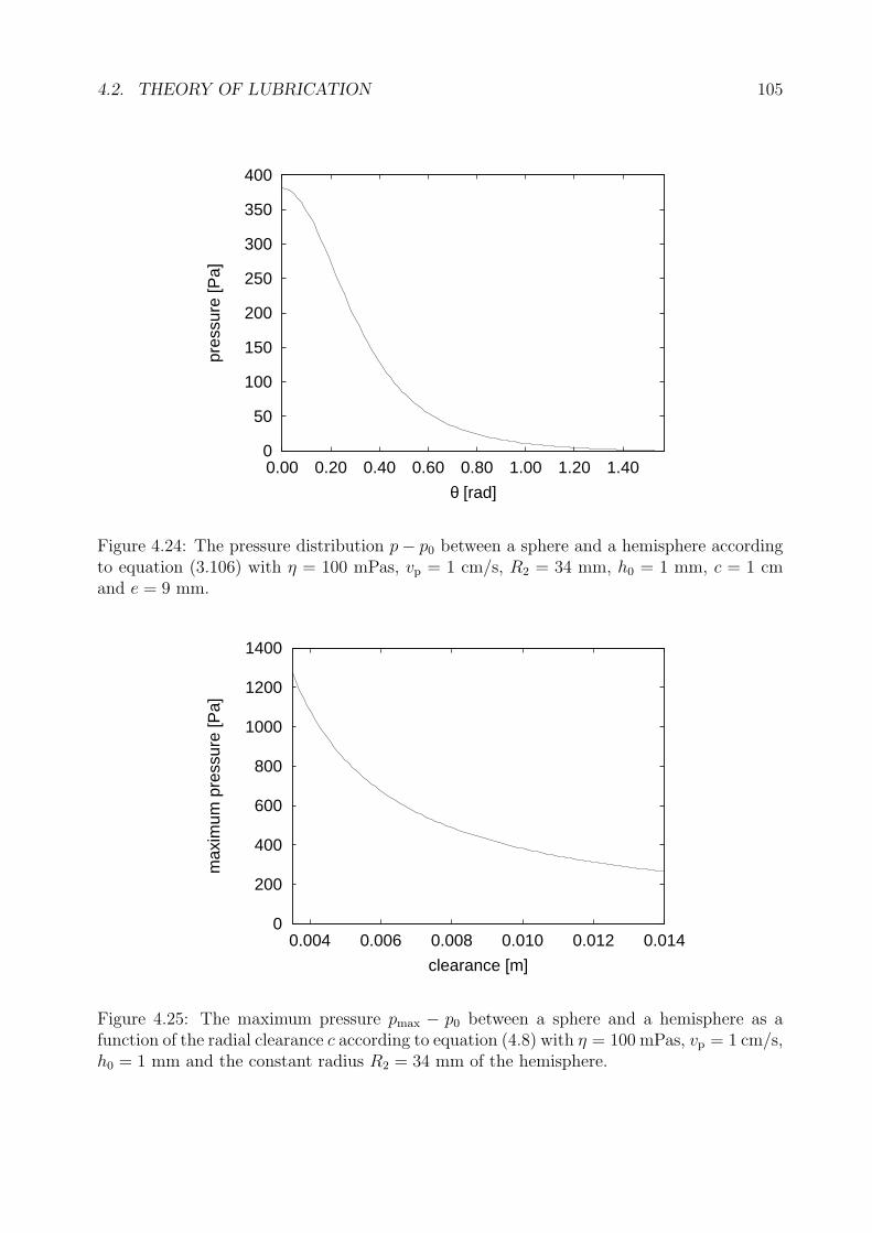
4.2. THEORY OF LUBRICATION 105
0
50
100
150
200
250
300
350
400
0.00 0.20 0.40 0.60 0.80 1.00 1.20 1.40
pres
sure
[Pa]
θ [rad]
Figure 4.24: The pressure distribution p− p0 between a sphere and a hemisphere accordingto equation (3.106) with η = 100 mPas, vp = 1 cm/s, R2 = 34 mm, h0 = 1 mm, c = 1 cmand e = 9 mm.
0
200
400
600
800
1000
1200
1400
0.004 0.006 0.008 0.010 0.012 0.014
max
imum
pre
ssur
e [P
a]
clearance [m]
Figure 4.25: The maximum pressure pmax − p0 between a sphere and a hemisphere as afunction of the radial clearance c according to equation (4.8) with η = 100 mPas, vp = 1 cm/s,h0 = 1 mm and the constant radius R2 = 34 mm of the hemisphere.
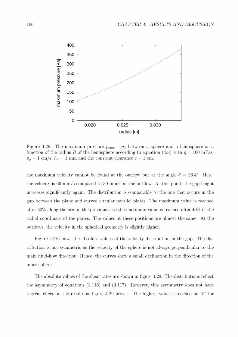
106 CHAPTER 4. RESULTS AND DISCUSSION
0
50
100
150
200
250
300
350
400
0.020 0.025 0.030
max
imum
pre
ssur
e [P
a]
radius [m]
Figure 4.26: The maximum pressure pmax − p0 between a sphere and a hemisphere as afunction of the radius R of the hemisphere according to equation (4.8) with η = 100 mPas,vp = 1 cm/s, h0 = 1 mm and the constant clearance c = 1 cm.
the maximum velocity cannot be found at the outflow but at the angle θ = 26.4◦. Here,
the velocity is 60 mm/s compared to 30 mm/s at the outflow. At this point, the gap height
increases significantly again. The distribution is comparable to the one that occurs in the
gap between the plane and curved circular parallel plates. The maximum value is reached
after 30% along the arc, in the previous case the maximum value is reached after 40% of the
radial coordinate of the plates. The values at these positions are almost the same. At the
outflows, the velocity in the spherical geometry is slightly higher.
Figure 4.28 shows the absolute values of the velocity distribution in the gap. The dis-
tribution is not symmetric as the velocity of the sphere is not always perpendicular to the
main fluid-flow direction. Hence, the curves show a small declination in the direction of the
inner sphere.
The absolute values of the shear rates are shown in figure 4.29. The distributions reflect
the asymmetry of equations (3.116) and (3.117). However, this asymmetry does not have
a great effect on the results as figure 4.29 proves. The highest value is reached at 15◦ for
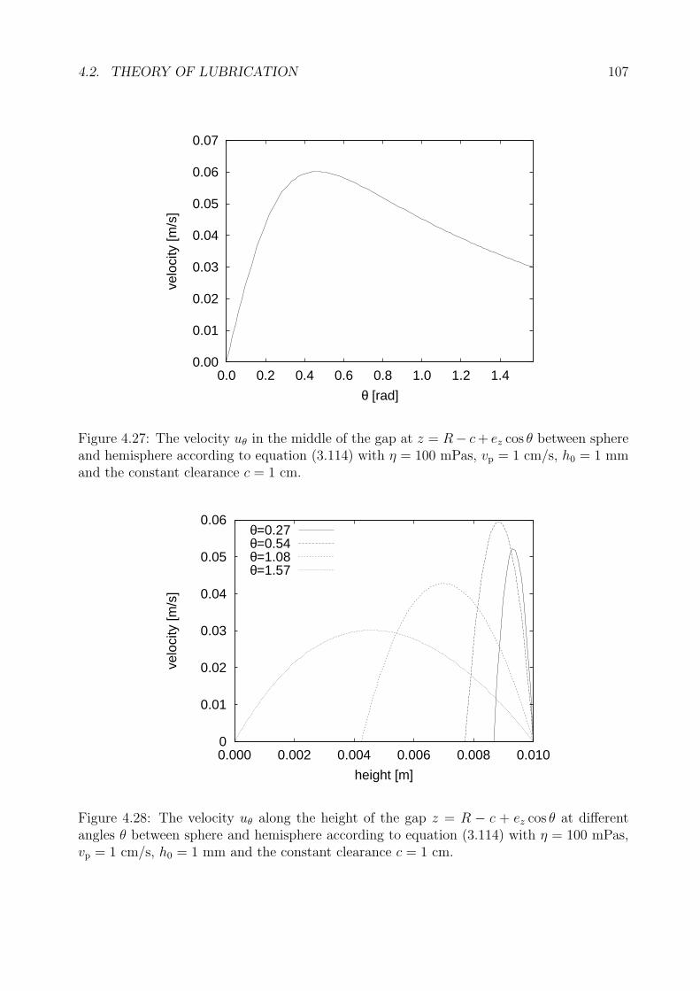
4.2. THEORY OF LUBRICATION 107
0.00
0.01
0.02
0.03
0.04
0.05
0.06
0.07
0.0 0.2 0.4 0.6 0.8 1.0 1.2 1.4
velo
city
[m/s
]
θ [rad]
Figure 4.27: The velocity uθ in the middle of the gap at z = R− c+ ez cos θ between sphereand hemisphere according to equation (3.114) with η = 100 mPas, vp = 1 cm/s, h0 = 1 mmand the constant clearance c = 1 cm.
0
0.01
0.02
0.03
0.04
0.05
0.06
0.000 0.002 0.004 0.006 0.008 0.010
velo
city
[m/s
]
height [m]
θ=0.27θ=0.54θ=1.08θ=1.57
Figure 4.28: The velocity uθ along the height of the gap z = R − c + ez cos θ at differentangles θ between sphere and hemisphere according to equation (3.114) with η = 100 mPas,vp = 1 cm/s, h0 = 1 mm and the constant clearance c = 1 cm.
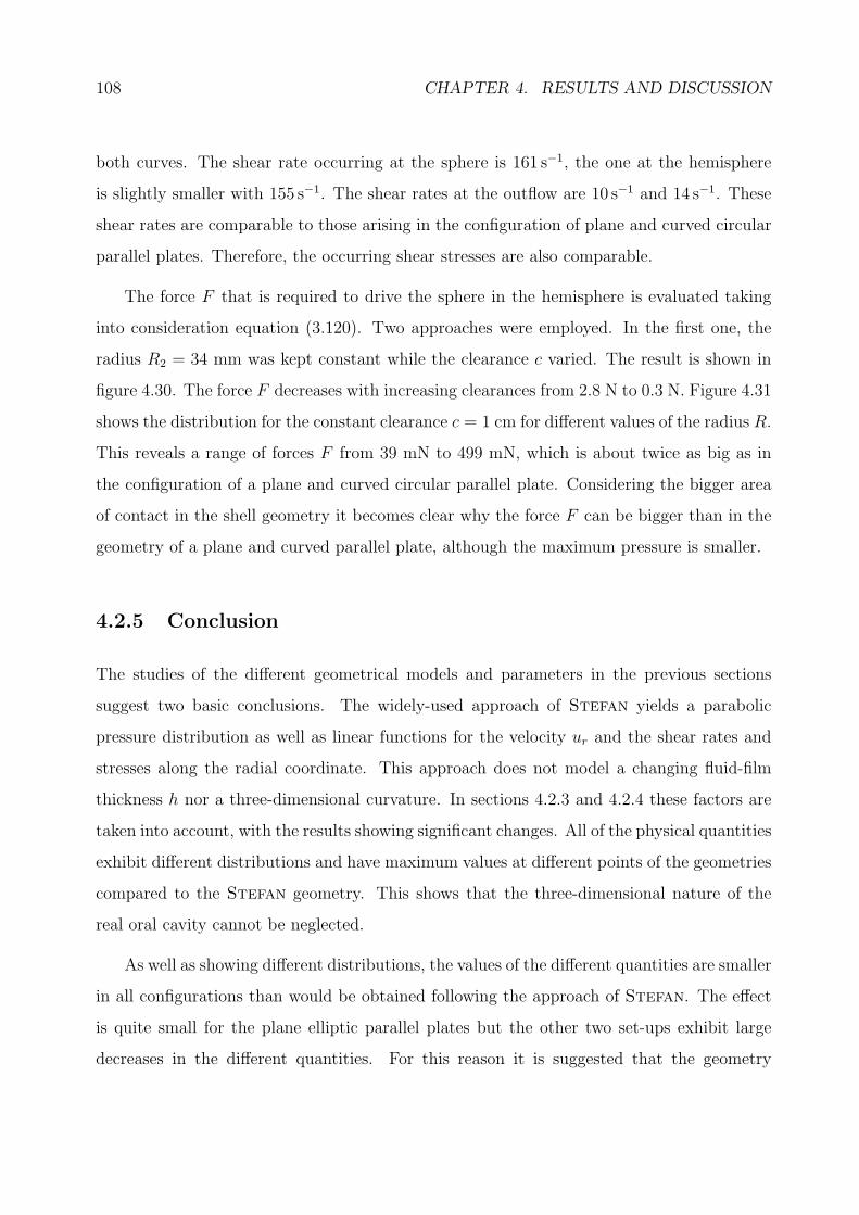
108 CHAPTER 4. RESULTS AND DISCUSSION
both curves. The shear rate occurring at the sphere is 161 s−1, the one at the hemisphere
is slightly smaller with 155 s−1. The shear rates at the outflow are 10 s−1 and 14 s−1. These
shear rates are comparable to those arising in the configuration of plane and curved circular
parallel plates. Therefore, the occurring shear stresses are also comparable.
The force F that is required to drive the sphere in the hemisphere is evaluated taking
into consideration equation (3.120). Two approaches were employed. In the first one, the
radius R2 = 34 mm was kept constant while the clearance c varied. The result is shown in
figure 4.30. The force F decreases with increasing clearances from 2.8 N to 0.3 N. Figure 4.31
shows the distribution for the constant clearance c = 1 cm for different values of the radius R.
This reveals a range of forces F from 39 mN to 499 mN, which is about twice as big as in
the configuration of a plane and curved circular parallel plate. Considering the bigger area
of contact in the shell geometry it becomes clear why the force F can be bigger than in the
geometry of a plane and curved parallel plate, although the maximum pressure is smaller.
4.2.5 Conclusion
The studies of the different geometrical models and parameters in the previous sections
suggest two basic conclusions. The widely-used approach of Stefan yields a parabolic
pressure distribution as well as linear functions for the velocity ur and the shear rates and
stresses along the radial coordinate. This approach does not model a changing fluid-film
thickness h nor a three-dimensional curvature. In sections 4.2.3 and 4.2.4 these factors are
taken into account, with the results showing significant changes. All of the physical quantities
exhibit different distributions and have maximum values at different points of the geometries
compared to the Stefan geometry. This shows that the three-dimensional nature of the
real oral cavity cannot be neglected.
As well as showing different distributions, the values of the different quantities are smaller
in all configurations than would be obtained following the approach of Stefan. The effect
is quite small for the plane elliptic parallel plates but the other two set-ups exhibit large
decreases in the different quantities. For this reason it is suggested that the geometry
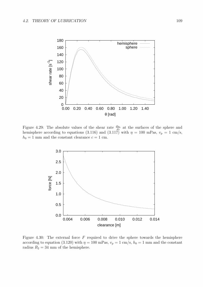
4.2. THEORY OF LUBRICATION 109
0
20
40
60
80
100
120
140
160
180
0.00 0.20 0.40 0.60 0.80 1.00 1.20 1.40
shea
r ra
te [s
-1]
θ [rad]
hemispheresphere
Figure 4.29: The absolute values of the shear rate dur
dzat the surfaces of the sphere and
hemisphere according to equations (3.116) and (3.117) with η = 100 mPas, vp = 1 cm/s,h0 = 1 mm and the constant clearance c = 1 cm.
0.0
0.5
1.0
1.5
2.0
2.5
3.0
0.004 0.006 0.008 0.010 0.012 0.014
forc
e [N
]
clearance [m]
Figure 4.30: The external force F required to drive the sphere towards the hemisphereaccording to equation (3.120) with η = 100 mPas, vp = 1 cm/s, h0 = 1 mm and the constantradius R2 = 34 mm of the hemisphere.

110 CHAPTER 4. RESULTS AND DISCUSSION
0.0
0.1
0.2
0.3
0.4
0.5
0.020 0.025 0.030
forc
e [N
]
radius [m]
Figure 4.31: The external force F required to drive the sphere in the hemisphere according toequation (3.120) with η = 100 mPas, vp = 1 cm/s, h0 = 1 mm and the constant clearance c =1 cm.
of two plane circular parallel plates should be handled with care when employing it as a
reference method for a squeezing flow in the oral cavity. It is advisable also to employ the
other configurations, especially the one of the sphere driving into a hemisphere, in order
to estimate the values of fluid-mechanical quantities in the mouth. This is significant in
terms the human mechanoreceptors as it suggests that they must be even more sensitive
than would be expected from the Stefan model.
4.3 Numerical Simulations
The numerical simulations generate three-dimensional data of flow fields. Figure 4.32 shows
the calculated pressure distribution for the cases N4 and CL from above. It is clear that the
results are qualitatively similar. The pressure has the highest value at the tip of the model
tongue in each case and decreases in the rear part of the model. Additionally, the isolines
of pressure have a parabolic form in both cases.
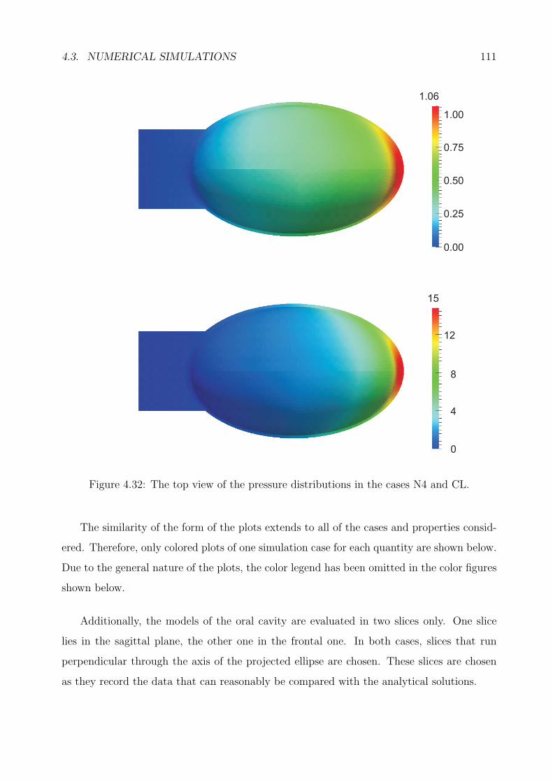
4.3. NUMERICAL SIMULATIONS 111
N4
CL
0.00
0.25
0.50
0.75
1.00
1.06
0
4
8
12
15
Figure 4.32: The top view of the pressure distributions in the cases N4 and CL.
The similarity of the form of the plots extends to all of the cases and properties consid-
ered. Therefore, only colored plots of one simulation case for each quantity are shown below.
Due to the general nature of the plots, the color legend has been omitted in the color figures
shown below.
Additionally, the models of the oral cavity are evaluated in two slices only. One slice
lies in the sagittal plane, the other one in the frontal one. In both cases, slices that run
perpendicular through the axis of the projected ellipse are chosen. These slices are chosen
as they record the data that can reasonably be compared with the analytical solutions.

112 CHAPTER 4. RESULTS AND DISCUSSION
The results in these slices are evaluated on the basis of representative points in which
the vector-field data are read out at the end of the simulation. One set of points lies directly
at the surface of the movable model tongue. The other set is located in the middle of the
bulk. Figure 4.33 shows this configuration exemplarily on the basis of the sagittal plane.
The origin of the x-axis is located at the outflow. The y-axis starts at the major axis of
the projected ellipse. The evaluation in the sagittal plane only starts from x = 0.03 m as
the radical changing of the geometry representing the pharynx causes abrupt changes in the
flow-field data.
4.3.1 Pressures
Figure 4.34 gives a qualitative impression of the pressure distribution in the bulk between
the movable model tongue and the fixed model palate. It is representative for all models
used in the current study and is independent from the implemented rheological model and
the related constants. The detailed evaluation with quantitative values takes place according
to the representative points introduced above.
Figure 4.35 shows the pressure distribution in the middle of the bulk and at the surface
of the model tongue in the sagittal plane using the example of case N4. This case was chosen
for reference as the analytical calculations in section 4.2 are based on the same viscosity.
The values occurring in the bulk and on the surface of the movable tongue do not alter
significantly. This is consistent with the assumptions made for the analytical derivation in
the theory of lubrication (section 3.3). As expected, the maximum pressures occur at the
tip of the model tongue. The qualitative distribution indeed resembles the distributions that
were found analytically in sections 4.2.3 and 4.2.4, which discuss squeezing flows between
plane and curved circular parallel plates and a sphere in a hemisphere.
The pressure drops rapidly until reaching a plateau in the vicinity of the center of the
projected ellipse. The level of this plateau lies at about half the maximum pressure for the
low viscosity cases N1, N2 and N3. The higher the viscosity, the more abrupt the decline is
before reaching the pressure plateau. In case N4, the pressure falls back to approximately
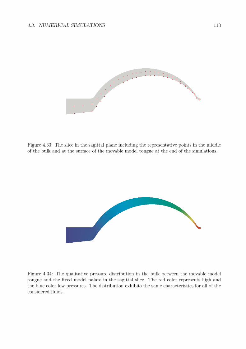
4.3. NUMERICAL SIMULATIONS 113
Figure 4.33: The slice in the sagittal plane including the representative points in the middleof the bulk and at the surface of the movable model tongue at the end of the simulations.
Figure 4.34: The qualitative pressure distribution in the bulk between the movable modeltongue and the fixed model palate in the sagittal slice. The red color represents high andthe blue color low pressures. The distribution exhibits the same characteristics for all of theconsidered fluids.
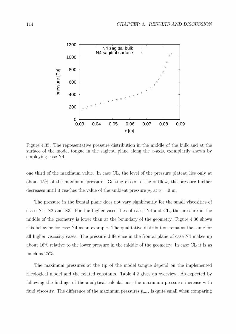
114 CHAPTER 4. RESULTS AND DISCUSSION
0
200
400
600
800
1000
1200
0.03 0.04 0.05 0.06 0.07 0.08 0.09
pres
sure
[Pa]
x [m]
N4 sagittal bulkN4 sagittal surface
Figure 4.35: The representative pressure distribution in the middle of the bulk and at thesurface of the model tongue in the sagittal plane along the x-axis, exemplarily shown byemploying case N4.
one third of the maximum value. In case CL, the level of the pressure plateau lies only at
about 15% of the maximum pressure. Getting closer to the outflow, the pressure further
decreases until it reaches the value of the ambient pressure p0 at x = 0 m.
The pressure in the frontal plane does not vary significantly for the small viscosities of
cases N1, N2 and N3. For the higher viscosities of cases N4 and CL, the pressure in the
middle of the geometry is lower than at the boundary of the geometry. Figure 4.36 shows
this behavior for case N4 as an example. The qualitative distribution remains the same for
all higher viscosity cases. The pressure difference in the frontal plane of case N4 makes up
about 16% relative to the lower pressure in the middle of the geometry. In case CL it is as
much as 25%.
The maximum pressures at the tip of the model tongue depend on the implemented
rheological model and the related constants. Table 4.2 gives an overview. As expected by
following the findings of the analytical calculations, the maximum pressures increase with
fluid viscosity. The difference of the maximum pressures pmax is quite small when comparing
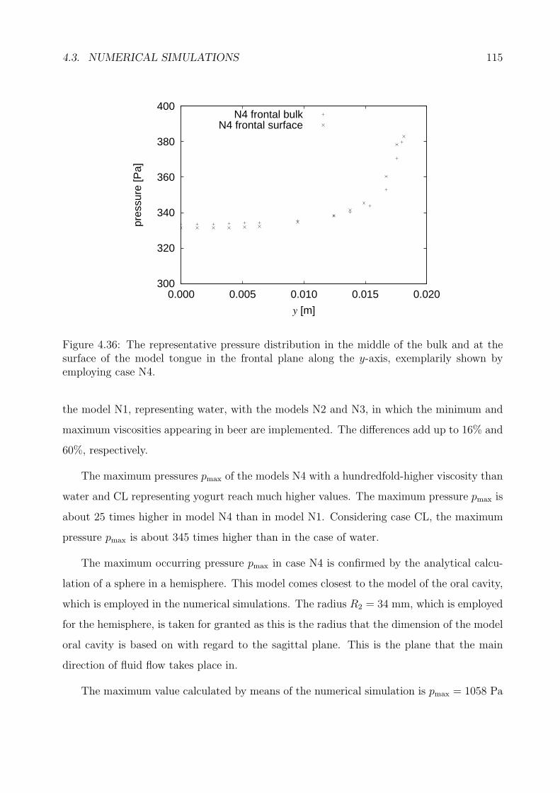
4.3. NUMERICAL SIMULATIONS 115
300
320
340
360
380
400
0.000 0.005 0.010 0.015 0.020
pres
sure
[Pa]
y [m]
N4 frontal bulkN4 frontal surface
Figure 4.36: The representative pressure distribution in the middle of the bulk and at thesurface of the model tongue in the frontal plane along the y-axis, exemplarily shown byemploying case N4.
the model N1, representing water, with the models N2 and N3, in which the minimum and
maximum viscosities appearing in beer are implemented. The differences add up to 16% and
60%, respectively.
The maximum pressures pmax of the models N4 with a hundredfold-higher viscosity than
water and CL representing yogurt reach much higher values. The maximum pressure pmax is
about 25 times higher in model N4 than in model N1. Considering case CL, the maximum
pressure pmax is about 345 times higher than in the case of water.
The maximum occurring pressure pmax in case N4 is confirmed by the analytical calcu-
lation of a sphere in a hemisphere. This model comes closest to the model of the oral cavity,
which is employed in the numerical simulations. The radius R2 = 34 mm, which is employed
for the hemisphere, is taken for granted as this is the radius that the dimension of the model
oral cavity is based on with regard to the sagittal plane. This is the plane that the main
direction of fluid flow takes place in.
The maximum value calculated by means of the numerical simulation is pmax = 1058 Pa
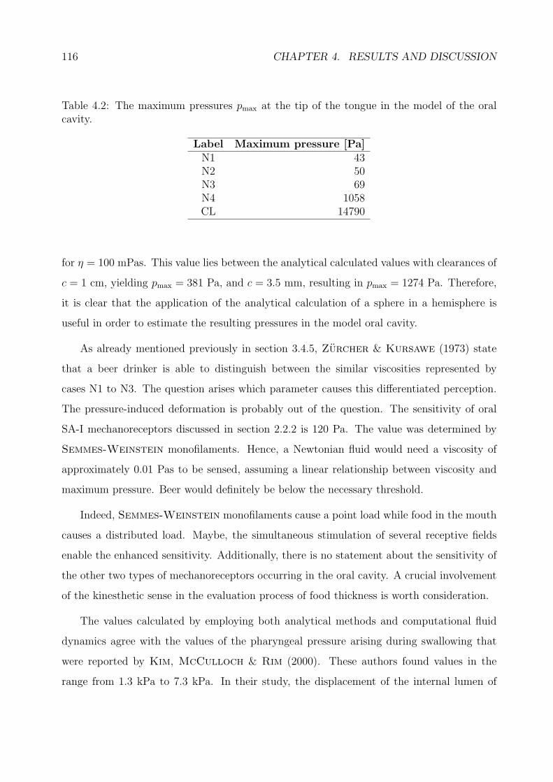
116 CHAPTER 4. RESULTS AND DISCUSSION
Table 4.2: The maximum pressures pmax at the tip of the tongue in the model of the oralcavity.
Label Maximum pressure [Pa]N1 43N2 50N3 69N4 1058CL 14790
for η = 100 mPas. This value lies between the analytical calculated values with clearances of
c = 1 cm, yielding pmax = 381 Pa, and c = 3.5 mm, resulting in pmax = 1274 Pa. Therefore,
it is clear that the application of the analytical calculation of a sphere in a hemisphere is
useful in order to estimate the resulting pressures in the model oral cavity.
As already mentioned previously in section 3.4.5, Zurcher & Kursawe (1973) state
that a beer drinker is able to distinguish between the similar viscosities represented by
cases N1 to N3. The question arises which parameter causes this differentiated perception.
The pressure-induced deformation is probably out of the question. The sensitivity of oral
SA-I mechanoreceptors discussed in section 2.2.2 is 120 Pa. The value was determined by
Semmes-Weinstein monofilaments. Hence, a Newtonian fluid would need a viscosity of
approximately 0.01 Pas to be sensed, assuming a linear relationship between viscosity and
maximum pressure. Beer would definitely be below the necessary threshold.
Indeed, Semmes-Weinstein monofilaments cause a point load while food in the mouth
causes a distributed load. Maybe, the simultaneous stimulation of several receptive fields
enable the enhanced sensitivity. Additionally, there is no statement about the sensitivity of
the other two types of mechanoreceptors occurring in the oral cavity. A crucial involvement
of the kinesthetic sense in the evaluation process of food thickness is worth consideration.
The values calculated by employing both analytical methods and computational fluid
dynamics agree with the values of the pharyngeal pressure arising during swallowing that
were reported by Kim, McCulloch & Rim (2000). These authors found values in the
range from 1.3 kPa to 7.3 kPa. In their study, the displacement of the internal lumen of
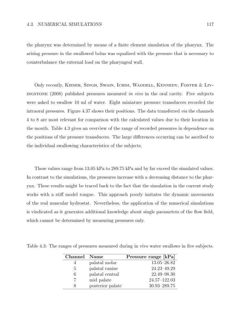
4.3. NUMERICAL SIMULATIONS 117
the pharynx was determined by means of a finite element simulation of the pharynx. The
arising pressure in the swallowed bolus was equalized with the pressure that is necessary to
counterbalance the external load on the pharyngeal wall.
Only recently, Kieser, Singh, Swain, Ichim, Waddell, Kennedy, Foster & Liv-
ingstone (2008) published pressures measured in vivo in the oral cavity. Five subjects
were asked to swallow 10 ml of water. Eight miniature pressure transducers recorded the
intraoral pressures. Figure 4.37 shows their positions. The data transferred via the channels
4 to 8 are most relevant for comparison with the calculated values due to their location in
the mouth. Table 4.3 gives an overview of the range of recorded pressures in dependence on
the positions of the pressure transducers. The large differences occurring can be ascribed to
the individual swallowing characteristics of the subjects.
These values range from 13.05 kPa to 289.75 kPa and by far exceed the simulated values.
In contrast to the simulations, the pressures increase with a decreasing distance to the phar-
ynx. These results might be traced back to the fact that the simulation in the current study
works with a stiff model tongue. This approach poorly imitates the dynamic movements
of the real muscular hydrostat. Nevertheless, the application of the numerical simulations
is vindicated as it generates additional knowledge about single parameters of the flow field,
which cannot be determined by measuring pressures only.
Table 4.3: The ranges of pressures measured during in vivo water swallows in five subjects.
Channel Name Pressure range [kPa]4 palatal molar 13.05–26.825 palatal canine 24.23–49.296 palatal central 22.49–98.307 mid palate 24.57–122.038 posterior palate 30.93–289.75
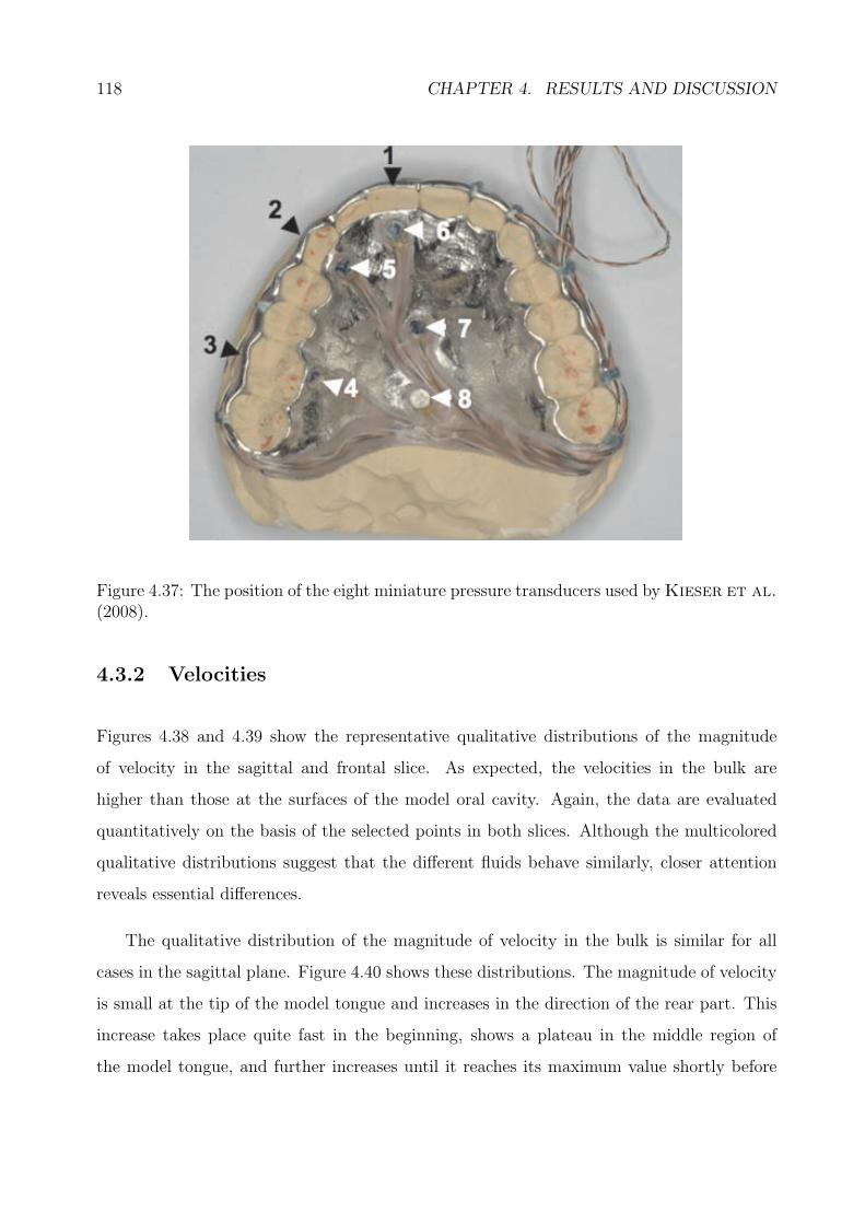
118 CHAPTER 4. RESULTS AND DISCUSSION
Figure 4.37: The position of the eight miniature pressure transducers used byKieser et al.(2008).
4.3.2 Velocities
Figures 4.38 and 4.39 show the representative qualitative distributions of the magnitude
of velocity in the sagittal and frontal slice. As expected, the velocities in the bulk are
higher than those at the surfaces of the model oral cavity. Again, the data are evaluated
quantitatively on the basis of the selected points in both slices. Although the multicolored
qualitative distributions suggest that the different fluids behave similarly, closer attention
reveals essential differences.
The qualitative distribution of the magnitude of velocity in the bulk is similar for all
cases in the sagittal plane. Figure 4.40 shows these distributions. The magnitude of velocity
is small at the tip of the model tongue and increases in the direction of the rear part. This
increase takes place quite fast in the beginning, shows a plateau in the middle region of
the model tongue, and further increases until it reaches its maximum value shortly before
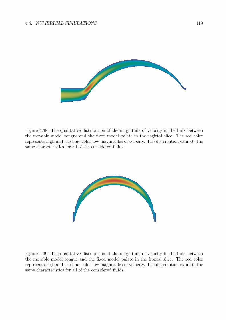
4.3. NUMERICAL SIMULATIONS 119
Figure 4.38: The qualitative distribution of the magnitude of velocity in the bulk betweenthe movable model tongue and the fixed model palate in the sagittal slice. The red colorrepresents high and the blue color low magnitudes of velocity. The distribution exhibits thesame characteristics for all of the considered fluids.
Figure 4.39: The qualitative distribution of the magnitude of velocity in the bulk betweenthe movable model tongue and the fixed model palate in the frontal slice. The red colorrepresents high and the blue color low magnitudes of velocity. The distribution exhibits thesame characteristics for all of the considered fluids.
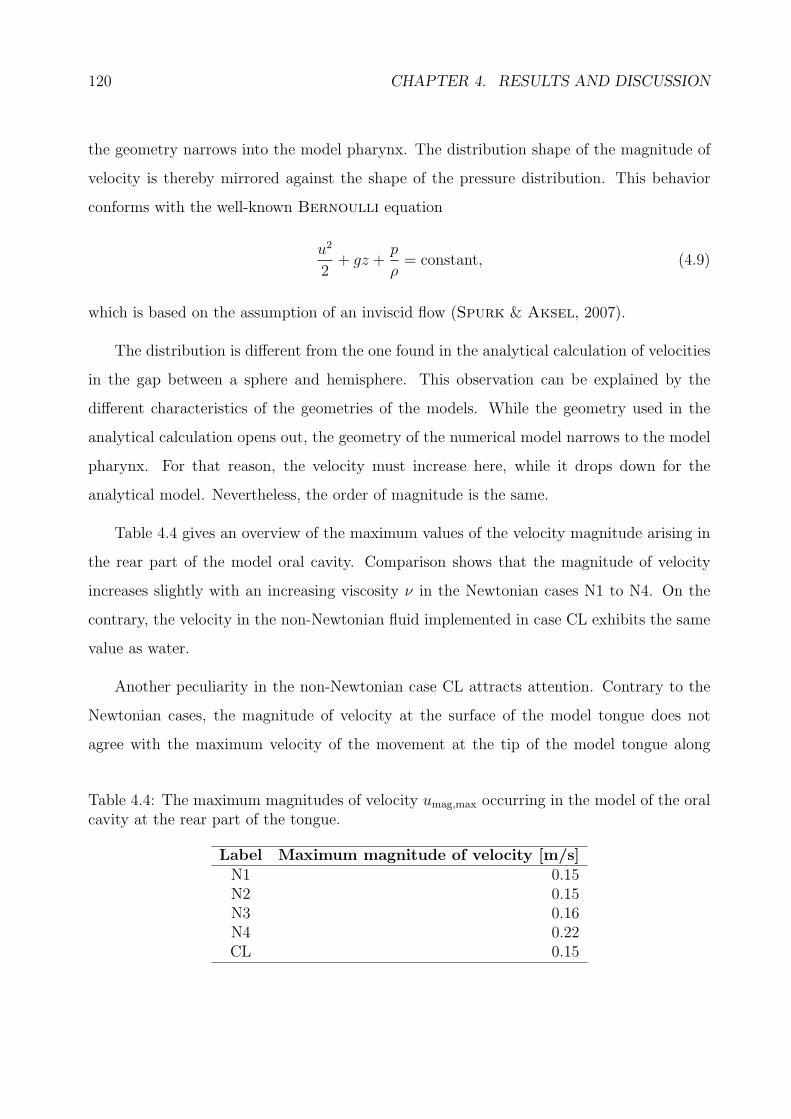
120 CHAPTER 4. RESULTS AND DISCUSSION
the geometry narrows into the model pharynx. The distribution shape of the magnitude of
velocity is thereby mirrored against the shape of the pressure distribution. This behavior
conforms with the well-known Bernoulli equation
u2
2+ gz +
p
ρ= constant, (4.9)
which is based on the assumption of an inviscid flow (Spurk & Aksel, 2007).
The distribution is different from the one found in the analytical calculation of velocities
in the gap between a sphere and hemisphere. This observation can be explained by the
different characteristics of the geometries of the models. While the geometry used in the
analytical calculation opens out, the geometry of the numerical model narrows to the model
pharynx. For that reason, the velocity must increase here, while it drops down for the
analytical model. Nevertheless, the order of magnitude is the same.
Table 4.4 gives an overview of the maximum values of the velocity magnitude arising in
the rear part of the model oral cavity. Comparison shows that the magnitude of velocity
increases slightly with an increasing viscosity ν in the Newtonian cases N1 to N4. On the
contrary, the velocity in the non-Newtonian fluid implemented in case CL exhibits the same
value as water.
Another peculiarity in the non-Newtonian case CL attracts attention. Contrary to the
Newtonian cases, the magnitude of velocity at the surface of the model tongue does not
agree with the maximum velocity of the movement at the tip of the model tongue along
Table 4.4: The maximum magnitudes of velocity umag,max occurring in the model of the oralcavity at the rear part of the tongue.
Label Maximum magnitude of velocity [m/s]N1 0.15N2 0.15N3 0.16N4 0.22CL 0.15
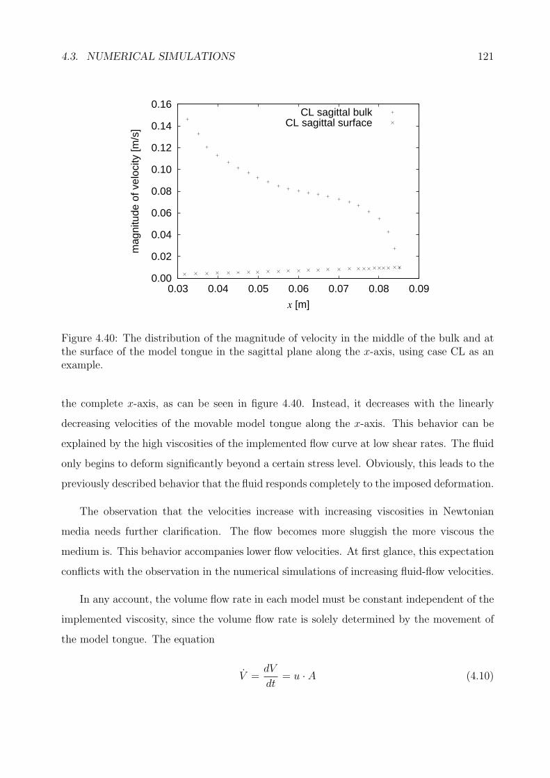
4.3. NUMERICAL SIMULATIONS 121
0.00
0.02
0.04
0.06
0.08
0.10
0.12
0.14
0.16
0.03 0.04 0.05 0.06 0.07 0.08 0.09
mag
nitu
de o
f vel
ocity
[m/s
]
x [m]
CL sagittal bulkCL sagittal surface
Figure 4.40: The distribution of the magnitude of velocity in the middle of the bulk and atthe surface of the model tongue in the sagittal plane along the x-axis, using case CL as anexample.
the complete x-axis, as can be seen in figure 4.40. Instead, it decreases with the linearly
decreasing velocities of the movable model tongue along the x-axis. This behavior can be
explained by the high viscosities of the implemented flow curve at low shear rates. The fluid
only begins to deform significantly beyond a certain stress level. Obviously, this leads to the
previously described behavior that the fluid responds completely to the imposed deformation.
The observation that the velocities increase with increasing viscosities in Newtonian
media needs further clarification. The flow becomes more sluggish the more viscous the
medium is. This behavior accompanies lower flow velocities. At first glance, this expectation
conflicts with the observation in the numerical simulations of increasing fluid-flow velocities.
In any account, the volume flow rate in each model must be constant independent of the
implemented viscosity, since the volume flow rate is solely determined by the movement of
the model tongue. The equation
V =dV
dt= u · A (4.10)
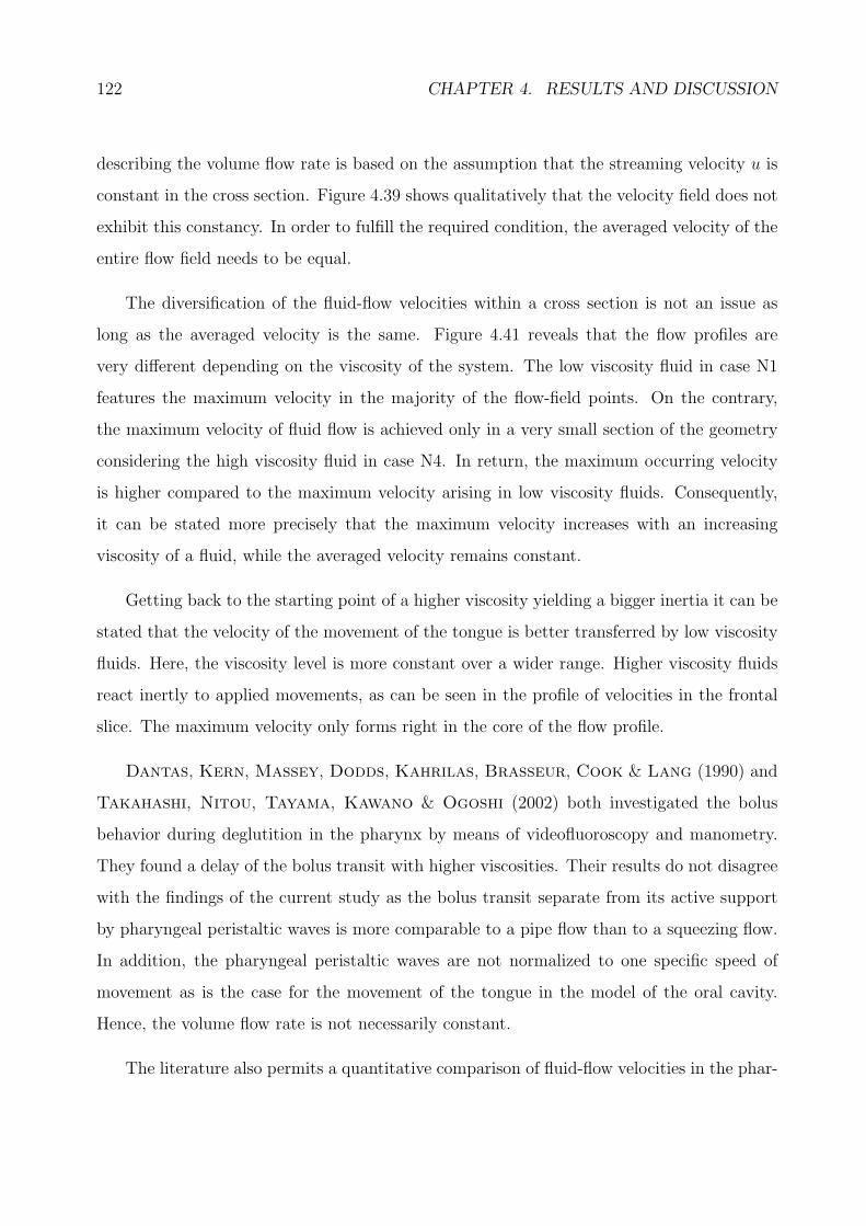
122 CHAPTER 4. RESULTS AND DISCUSSION
describing the volume flow rate is based on the assumption that the streaming velocity u is
constant in the cross section. Figure 4.39 shows qualitatively that the velocity field does not
exhibit this constancy. In order to fulfill the required condition, the averaged velocity of the
entire flow field needs to be equal.
The diversification of the fluid-flow velocities within a cross section is not an issue as
long as the averaged velocity is the same. Figure 4.41 reveals that the flow profiles are
very different depending on the viscosity of the system. The low viscosity fluid in case N1
features the maximum velocity in the majority of the flow-field points. On the contrary,
the maximum velocity of fluid flow is achieved only in a very small section of the geometry
considering the high viscosity fluid in case N4. In return, the maximum occurring velocity
is higher compared to the maximum velocity arising in low viscosity fluids. Consequently,
it can be stated more precisely that the maximum velocity increases with an increasing
viscosity of a fluid, while the averaged velocity remains constant.
Getting back to the starting point of a higher viscosity yielding a bigger inertia it can be
stated that the velocity of the movement of the tongue is better transferred by low viscosity
fluids. Here, the viscosity level is more constant over a wider range. Higher viscosity fluids
react inertly to applied movements, as can be seen in the profile of velocities in the frontal
slice. The maximum velocity only forms right in the core of the flow profile.
Dantas, Kern, Massey, Dodds, Kahrilas, Brasseur, Cook & Lang (1990) and
Takahashi, Nitou, Tayama, Kawano & Ogoshi (2002) both investigated the bolus
behavior during deglutition in the pharynx by means of videofluoroscopy and manometry.
They found a delay of the bolus transit with higher viscosities. Their results do not disagree
with the findings of the current study as the bolus transit separate from its active support
by pharyngeal peristaltic waves is more comparable to a pipe flow than to a squeezing flow.
In addition, the pharyngeal peristaltic waves are not normalized to one specific speed of
movement as is the case for the movement of the tongue in the model of the oral cavity.
Hence, the volume flow rate is not necessarily constant.
The literature also permits a quantitative comparison of fluid-flow velocities in the phar-
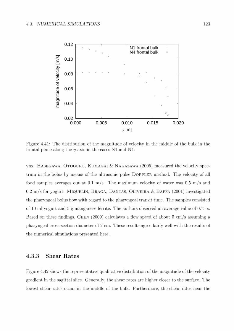
4.3. NUMERICAL SIMULATIONS 123
0.02
0.04
0.06
0.08
0.10
0.12
0.000 0.005 0.010 0.015 0.020
mag
nitu
de o
f vel
ocity
[m/s
]
y [m]
N1 frontal bulkN4 frontal bulk
Figure 4.41: The distribution of the magnitude of velocity in the middle of the bulk in thefrontal plane along the y-axis in the cases N1 and N4.
ynx. Hasegawa, Otoguro, Kumagai & Nakazawa (2005) measured the velocity spec-
trum in the bolus by means of the ultrasonic pulse Doppler method. The velocity of all
food samples averages out at 0.1 m/s. The maximum velocity of water was 0.5 m/s and
0.2 m/s for yogurt. Miquelin, Braga, Dantas, Oliveira & Baffa (2001) investigated
the pharyngeal bolus flow with regard to the pharyngeal transit time. The samples consisted
of 10 ml yogurt and 5 g manganese ferrite. The authors observed an average value of 0.75 s.
Based on these findings, Chen (2009) calculates a flow speed of about 5 cm/s assuming a
pharyngeal cross-section diameter of 2 cm. These results agree fairly well with the results of
the numerical simulations presented here.
4.3.3 Shear Rates
Figure 4.42 shows the representative qualitative distribution of the magnitude of the velocity
gradient in the sagittal slice. Generally, the shear rates are higher closer to the surface. The
lowest shear rates occur in the middle of the bulk. Furthermore, the shear rates near the
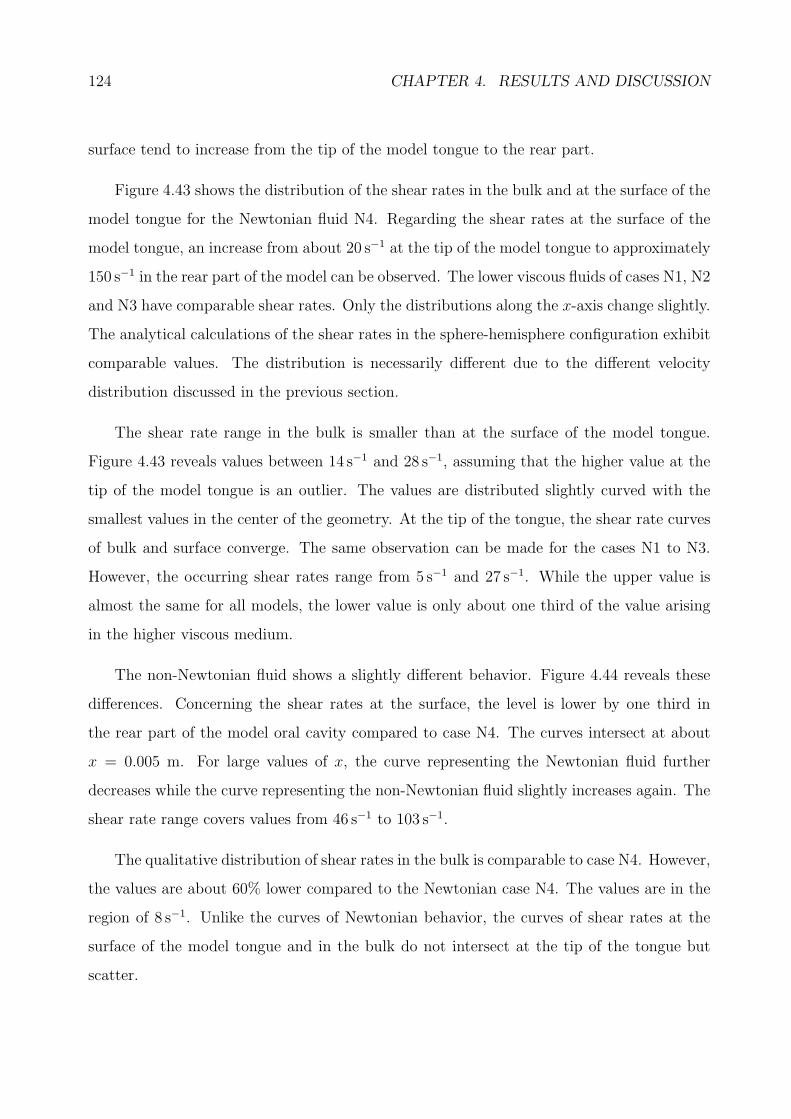
124 CHAPTER 4. RESULTS AND DISCUSSION
surface tend to increase from the tip of the model tongue to the rear part.
Figure 4.43 shows the distribution of the shear rates in the bulk and at the surface of the
model tongue for the Newtonian fluid N4. Regarding the shear rates at the surface of the
model tongue, an increase from about 20 s−1 at the tip of the model tongue to approximately
150 s−1 in the rear part of the model can be observed. The lower viscous fluids of cases N1, N2
and N3 have comparable shear rates. Only the distributions along the x-axis change slightly.
The analytical calculations of the shear rates in the sphere-hemisphere configuration exhibit
comparable values. The distribution is necessarily different due to the different velocity
distribution discussed in the previous section.
The shear rate range in the bulk is smaller than at the surface of the model tongue.
Figure 4.43 reveals values between 14 s−1 and 28 s−1, assuming that the higher value at the
tip of the model tongue is an outlier. The values are distributed slightly curved with the
smallest values in the center of the geometry. At the tip of the tongue, the shear rate curves
of bulk and surface converge. The same observation can be made for the cases N1 to N3.
However, the occurring shear rates range from 5 s−1 and 27 s−1. While the upper value is
almost the same for all models, the lower value is only about one third of the value arising
in the higher viscous medium.
The non-Newtonian fluid shows a slightly different behavior. Figure 4.44 reveals these
differences. Concerning the shear rates at the surface, the level is lower by one third in
the rear part of the model oral cavity compared to case N4. The curves intersect at about
x = 0.005 m. For large values of x, the curve representing the Newtonian fluid further
decreases while the curve representing the non-Newtonian fluid slightly increases again. The
shear rate range covers values from 46 s−1 to 103 s−1.
The qualitative distribution of shear rates in the bulk is comparable to case N4. However,
the values are about 60% lower compared to the Newtonian case N4. The values are in the
region of 8 s−1. Unlike the curves of Newtonian behavior, the curves of shear rates at the
surface of the model tongue and in the bulk do not intersect at the tip of the tongue but
scatter.
4.3. NUMERICAL SIMULATIONS 125
Figure 4.42: The qualitative distribution of the gradient of the magnitude of velocity in thebulk between the movable model tongue and the fixed model palate in the sagittal slice. Thered color represents high and the blue color low gradients of the velocity magnitude. Thedistribution exhibits the same characteristics for all of the considered fluids.
0
20
40
60
80
100
120
140
160
0.03 0.04 0.05 0.06 0.07 0.08 0.09
mag
nitu
de o
f gra
dien
t of v
eloc
ity [
s-1]
x [m]
N4 sagittal bulkN4 sagittal surface
Figure 4.43: The distribution of the magnitude of the gradient of velocity in the middle ofthe bulk and at the surface of the model tongue in the sagittal plane along the x-axis, forNewtonian fluids using case N4 as an example.
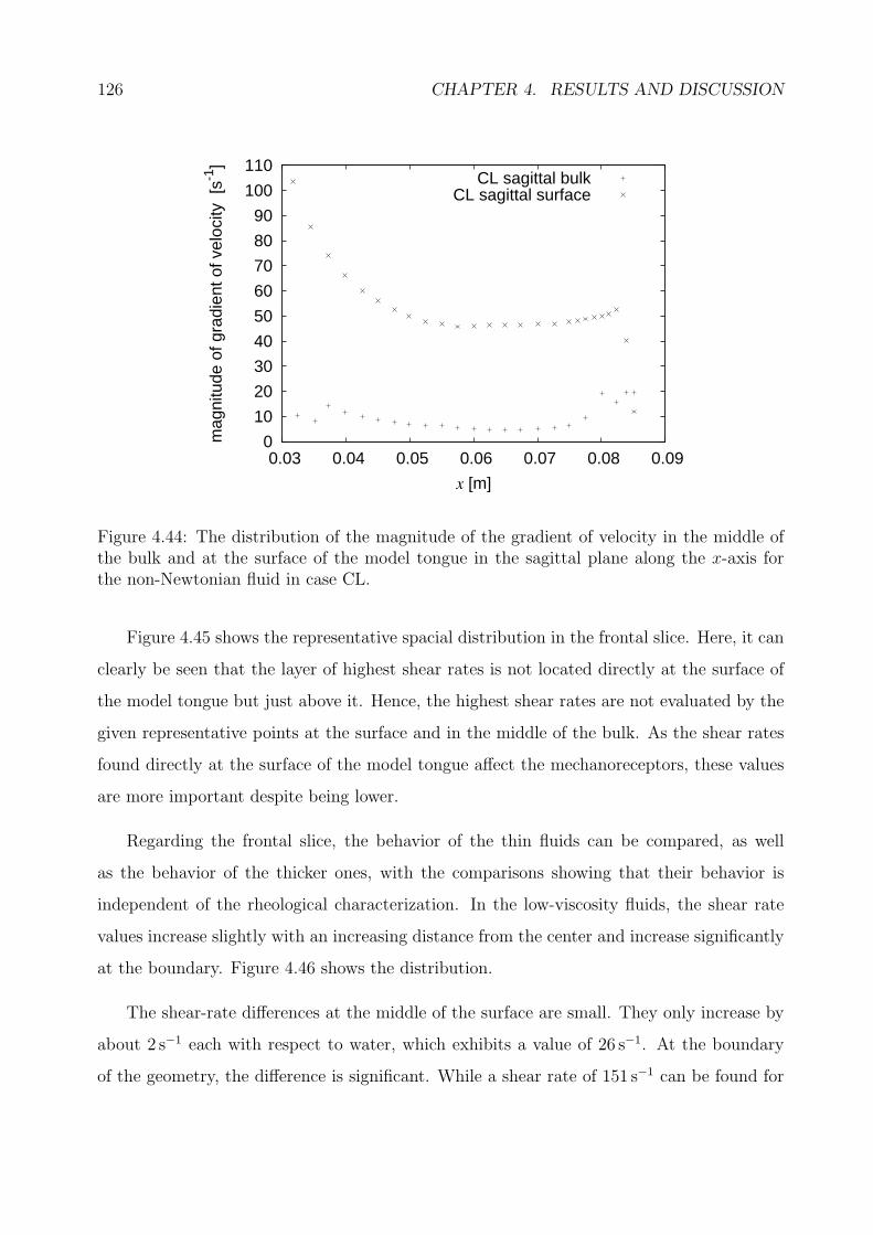
126 CHAPTER 4. RESULTS AND DISCUSSION
0
10
20
30
40
50
60
70
80
90
100
110
0.03 0.04 0.05 0.06 0.07 0.08 0.09
mag
nitu
de o
f gra
dien
t of v
eloc
ity [
s-1]
x [m]
CL sagittal bulkCL sagittal surface
Figure 4.44: The distribution of the magnitude of the gradient of velocity in the middle ofthe bulk and at the surface of the model tongue in the sagittal plane along the x-axis forthe non-Newtonian fluid in case CL.
Figure 4.45 shows the representative spacial distribution in the frontal slice. Here, it can
clearly be seen that the layer of highest shear rates is not located directly at the surface of
the model tongue but just above it. Hence, the highest shear rates are not evaluated by the
given representative points at the surface and in the middle of the bulk. As the shear rates
found directly at the surface of the model tongue affect the mechanoreceptors, these values
are more important despite being lower.
Regarding the frontal slice, the behavior of the thin fluids can be compared, as well
as the behavior of the thicker ones, with the comparisons showing that their behavior is
independent of the rheological characterization. In the low-viscosity fluids, the shear rate
values increase slightly with an increasing distance from the center and increase significantly
at the boundary. Figure 4.46 shows the distribution.
The shear-rate differences at the middle of the surface are small. They only increase by
about 2 s−1 each with respect to water, which exhibits a value of 26 s−1. At the boundary
of the geometry, the difference is significant. While a shear rate of 151 s−1 can be found for
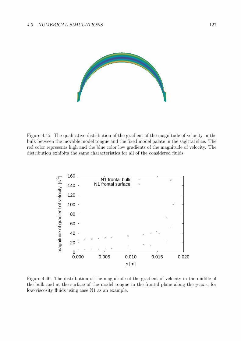
4.3. NUMERICAL SIMULATIONS 127
Figure 4.45: The qualitative distribution of the gradient of the magnitude of velocity in thebulk between the movable model tongue and the fixed model palate in the sagittal slice. Thered color represents high and the blue color low gradients of the magnitude of velocity. Thedistribution exhibits the same characteristics for all of the considered fluids.
0
20
40
60
80
100
120
140
160
0.000 0.005 0.010 0.015 0.020
mag
nitu
de o
f gra
dien
t of v
eloc
ity [
s-1]
y [m]
N1 frontal bulkN1 frontal surface
Figure 4.46: The distribution of the magnitude of the gradient of velocity in the middle ofthe bulk and at the surface of the model tongue in the frontal plane along the y-axis, forlow-viscosity fluids using case N1 as an example.
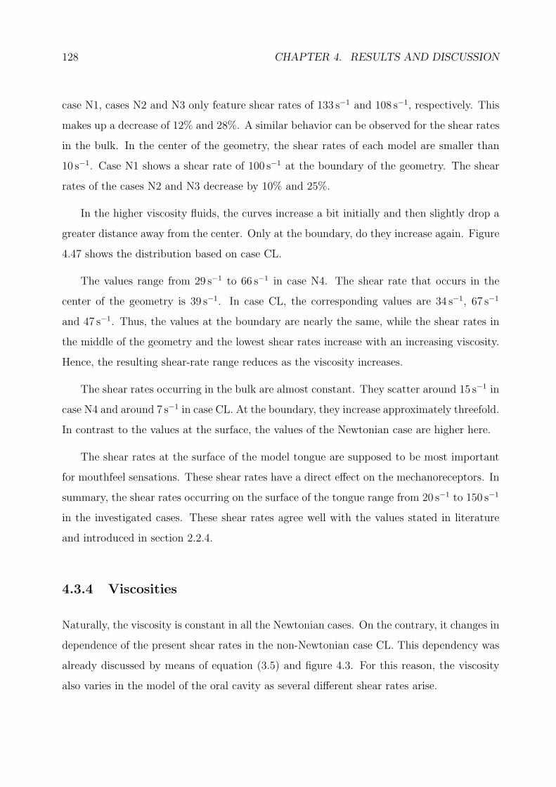
128 CHAPTER 4. RESULTS AND DISCUSSION
case N1, cases N2 and N3 only feature shear rates of 133 s−1 and 108 s−1, respectively. This
makes up a decrease of 12% and 28%. A similar behavior can be observed for the shear rates
in the bulk. In the center of the geometry, the shear rates of each model are smaller than
10 s−1. Case N1 shows a shear rate of 100 s−1 at the boundary of the geometry. The shear
rates of the cases N2 and N3 decrease by 10% and 25%.
In the higher viscosity fluids, the curves increase a bit initially and then slightly drop a
greater distance away from the center. Only at the boundary, do they increase again. Figure
4.47 shows the distribution based on case CL.
The values range from 29 s−1 to 66 s−1 in case N4. The shear rate that occurs in the
center of the geometry is 39 s−1. In case CL, the corresponding values are 34 s−1, 67 s−1
and 47 s−1. Thus, the values at the boundary are nearly the same, while the shear rates in
the middle of the geometry and the lowest shear rates increase with an increasing viscosity.
Hence, the resulting shear-rate range reduces as the viscosity increases.
The shear rates occurring in the bulk are almost constant. They scatter around 15 s−1 in
case N4 and around 7 s−1 in case CL. At the boundary, they increase approximately threefold.
In contrast to the values at the surface, the values of the Newtonian case are higher here.
The shear rates at the surface of the model tongue are supposed to be most important
for mouthfeel sensations. These shear rates have a direct effect on the mechanoreceptors. In
summary, the shear rates occurring on the surface of the tongue range from 20 s−1 to 150 s−1
in the investigated cases. These shear rates agree well with the values stated in literature
and introduced in section 2.2.4.
4.3.4 Viscosities
Naturally, the viscosity is constant in all the Newtonian cases. On the contrary, it changes in
dependence of the present shear rates in the non-Newtonian case CL. This dependency was
already discussed by means of equation (3.5) and figure 4.3. For this reason, the viscosity
also varies in the model of the oral cavity as several different shear rates arise.
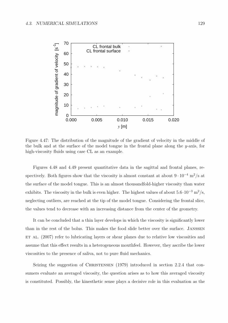
4.3. NUMERICAL SIMULATIONS 129
0
10
20
30
40
50
60
70
0.000 0.005 0.010 0.015 0.020
mag
nitu
de o
f gra
dien
t of v
eloc
ity [
s-1]
y [m]
CL frontal bulkCL frontal surface
Figure 4.47: The distribution of the magnitude of the gradient of velocity in the middle ofthe bulk and at the surface of the model tongue in the frontal plane along the y-axis, forhigh-viscosity fluids using case CL as an example.
Figures 4.48 and 4.49 present quantitative data in the sagittal and frontal planes, re-
spectively. Both figures show that the viscosity is almost constant at about 9 · 10−4 m2/s at
the surface of the model tongue. This is an almost thousandfold-higher viscosity than water
exhibits. The viscosity in the bulk is even higher. The highest values of about 5.6·10−3 m2/s,
neglecting outliers, are reached at the tip of the model tongue. Considering the frontal slice,
the values tend to decrease with an increasing distance from the center of the geometry.
It can be concluded that a thin layer develops in which the viscosity is significantly lower
than in the rest of the bolus. This makes the food slide better over the surface. Janssen
et al. (2007) refer to lubricating layers or shear planes due to relative low viscosities and
assume that this effect results in a heterogeneous mouthfeel. However, they ascribe the lower
viscosities to the presence of saliva, not to pure fluid mechanics.
Seizing the suggestion of Christensen (1979) introduced in section 2.2.4 that con-
sumers evaluate an averaged viscosity, the question arises as to how this averaged viscosity
is constituted. Possibly, the kinesthetic sense plays a decisive role in this evaluation as the
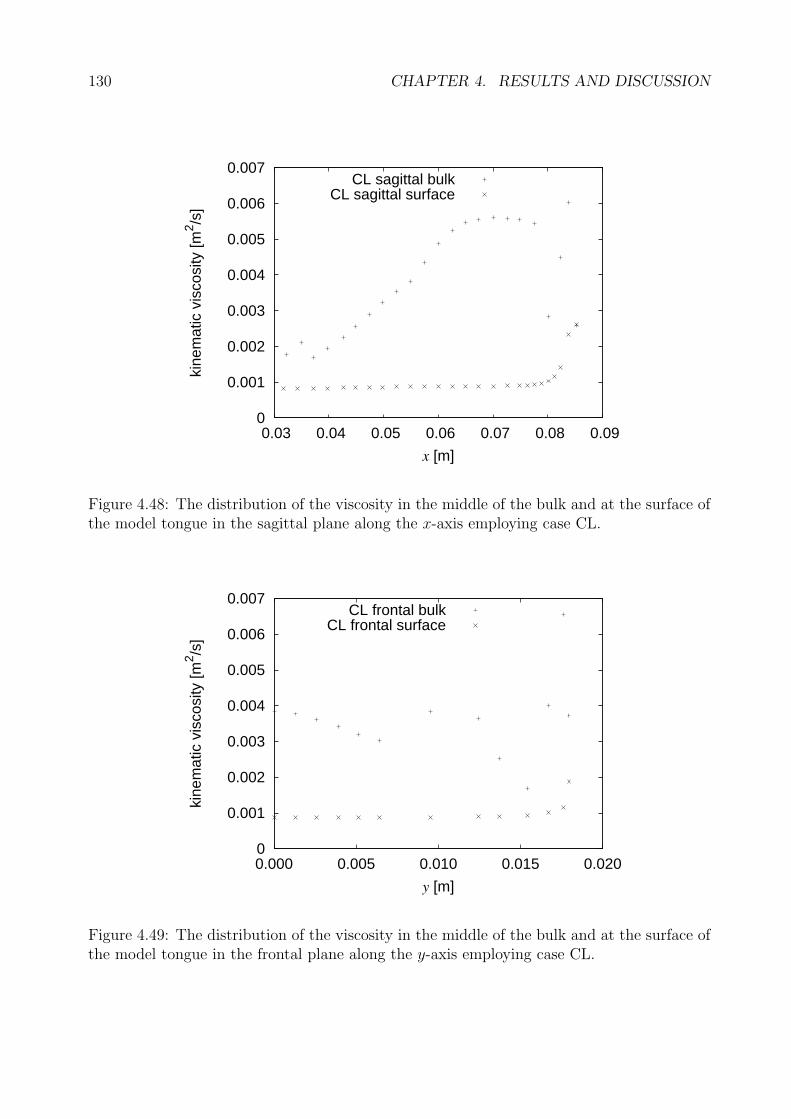
130 CHAPTER 4. RESULTS AND DISCUSSION
0
0.001
0.002
0.003
0.004
0.005
0.006
0.007
0.03 0.04 0.05 0.06 0.07 0.08 0.09
kine
mat
ic v
isco
sity
[m2 /s
]
x [m]
CL sagittal bulkCL sagittal surface
Figure 4.48: The distribution of the viscosity in the middle of the bulk and at the surface ofthe model tongue in the sagittal plane along the x-axis employing case CL.
0
0.001
0.002
0.003
0.004
0.005
0.006
0.007
0.000 0.005 0.010 0.015 0.020
kine
mat
ic v
isco
sity
[m2 /s
]
y [m]
CL frontal bulkCL frontal surface
Figure 4.49: The distribution of the viscosity in the middle of the bulk and at the surface ofthe model tongue in the frontal plane along the y-axis employing case CL.
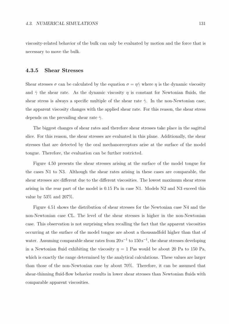
4.3. NUMERICAL SIMULATIONS 131
viscosity-related behavior of the bulk can only be evaluated by motion and the force that is
necessary to move the bulk.
4.3.5 Shear Stresses
Shear stresses σ can be calculated by the equation σ = ηγ where η is the dynamic viscosity
and γ the shear rate. As the dynamic viscosity η is constant for Newtonian fluids, the
shear stress is always a specific multiple of the shear rate γ. In the non-Newtonian case,
the apparent viscosity changes with the applied shear rate. For this reason, the shear stress
depends on the prevailing shear rate γ.
The biggest changes of shear rates and therefore shear stresses take place in the sagittal
slice. For this reason, the shear stresses are evaluated in this plane. Additionally, the shear
stresses that are detected by the oral mechanoreceptors arise at the surface of the model
tongue. Therefore, the evaluation can be further restricted.
Figure 4.50 presents the shear stresses arising at the surface of the model tongue for
the cases N1 to N3. Although the shear rates arising in these cases are comparable, the
shear stresses are different due to the different viscosities. The lowest maximum shear stress
arising in the rear part of the model is 0.15 Pa in case N1. Models N2 and N3 exceed this
value by 53% and 207%.
Figure 4.51 shows the distribution of shear stresses for the Newtonian case N4 and the
non-Newtonian case CL. The level of the shear stresses is higher in the non-Newtonian
case. This observation is not surprising when recalling the fact that the apparent viscosities
occurring at the surface of the model tongue are about a thousandfold higher than that of
water. Assuming comparable shear rates from 20 s−1 to 150 s−1, the shear stresses developing
in a Newtonian fluid exhibiting the viscosity η = 1 Pas would be about 20 Pa to 150 Pa,
which is exactly the range determined by the analytical calculations. These values are larger
than those of the non-Newtonian case by about 70%. Therefore, it can be assumed that
shear-thinning fluid-flow behavior results in lower shear stresses than Newtonian fluids with
comparable apparent viscosities.
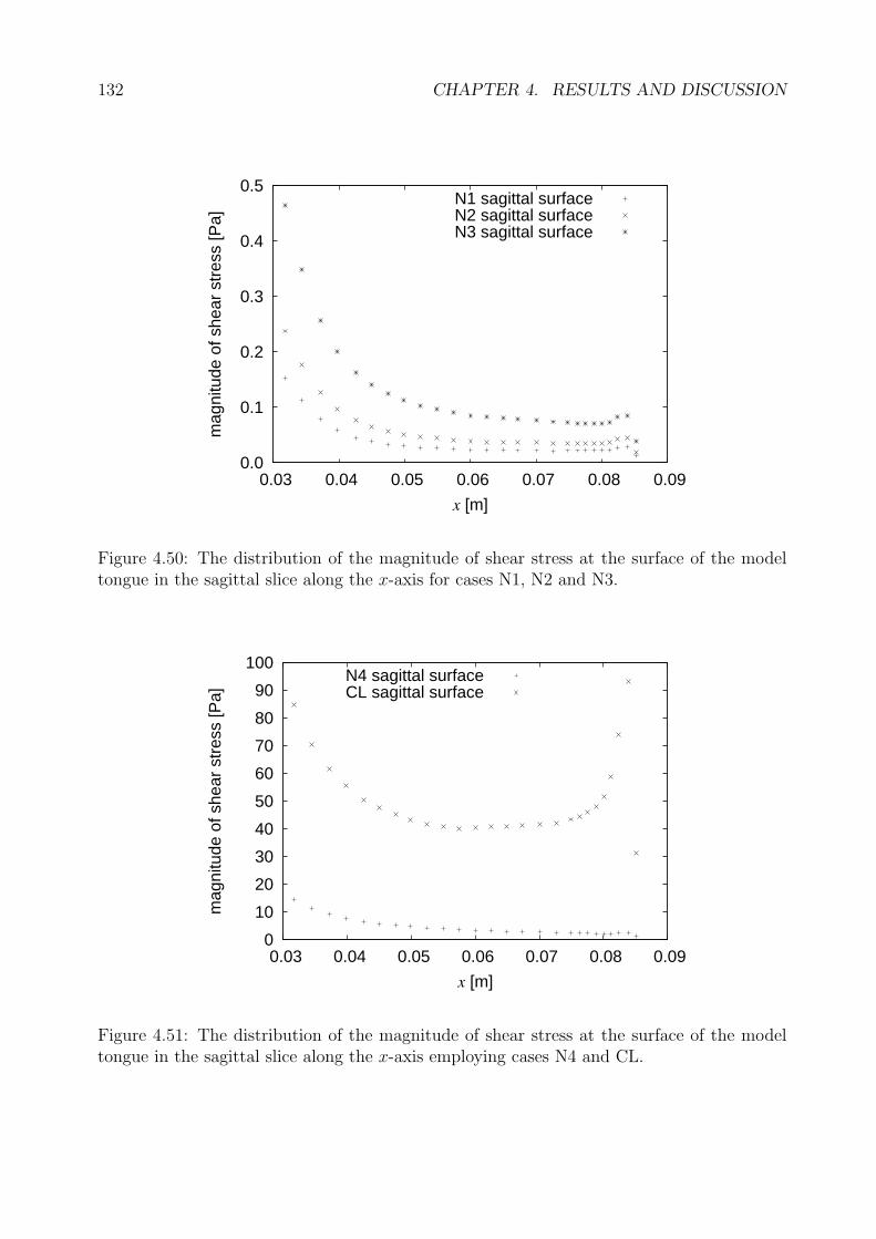
132 CHAPTER 4. RESULTS AND DISCUSSION
0.0
0.1
0.2
0.3
0.4
0.5
0.03 0.04 0.05 0.06 0.07 0.08 0.09
mag
nitu
de o
f she
ar s
tres
s [P
a]
x [m]
N1 sagittal surfaceN2 sagittal surfaceN3 sagittal surface
Figure 4.50: The distribution of the magnitude of shear stress at the surface of the modeltongue in the sagittal slice along the x-axis for cases N1, N2 and N3.
0
10
20
30
40
50
60
70
80
90
100
0.03 0.04 0.05 0.06 0.07 0.08 0.09
mag
nitu
de o
f she
ar s
tres
s [P
a]
x [m]
N4 sagittal surfaceCL sagittal surface
Figure 4.51: The distribution of the magnitude of shear stress at the surface of the modeltongue in the sagittal slice along the x-axis employing cases N4 and CL.
4.4. SUMMARY OF ANALYTICAL AND NUMERICAL FINDINGS 133
Apart from this result, non-Newtonian fluids exhibit a different shear-stress distribution
along the x-axis. While the shear stresses increase from the tip of the model tongue to
its rear part in Newtonian cases, the shear-rate distribution in the non-Newtonian case is
U-shaped due to the altering viscosities. The shear rates near the center of the geometry
stay at about 40 Pa, the shear rates at the tip of the model tongue and in the rear part are
more than twice as high.
The findings can be compared with the results from the literature presented in section
2.2.4. The previously reported shear-stress ranges amount to 10 Pa to 1000 Pa in general,
4.4 Pa to 131 Pa for syrups, 1 Pa for fresh milk and 683 Pa for chocolate spread. Although
the results from the numerical simulation exhibit a smaller minimum value, the order of
magnitude agrees well with previous findings.
4.4 Summary of Analytical and Numerical Findings
In the preceding sections novel approaches to investigate the fluid mechanics in the oral
cavity during deglutition and the resulting values for different physical quantities have been
presented. Table 4.5 compares selected findings from the current analytical and numerical
studies as well as the results of previous studies from literature. As the results of the
different analytical models and the numerical simulations in the present work take the form of
distributions, for comparison with the literature results the maximum value of each quantity
for a range of different geometry sizes has been given. The numerical values are taken from
case N4, as its viscosity is the same as the one used in the analytical considerations. The
physical quantities that are presented are the pressure, velocity, shear rate and shear stress.
It can be seen that the analytical and numerical approaches yield similar results, a strong
indication of the merits of the two approaches. Their favorable comparison with the literature
values is also very encouraging. Hence, the discussed analytical and numerical models offer
new possibilities to emulate the fluid flow between the human tongue and palate.
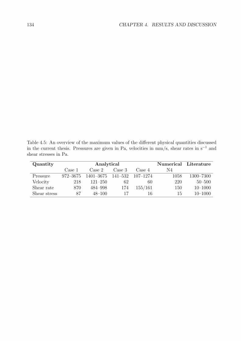
134 CHAPTER 4. RESULTS AND DISCUSSION
Table 4.5: An overview of the maximum values of the different physical quantities discussedin the current thesis. Pressures are given in Pa, velocities in mm/s, shear rates in s−1 andshear stresses in Pa.
Quantity Analytical Numerical LiteratureCase 1 Case 2 Case 3 Case 4 N4
Pressure 972–3675 1401–3675 141–532 107–1274 1058 1300–7300Velocity 218 121–250 62 60 220 50–500Shear rate 870 484–998 174 155/161 150 10–1000Shear stress 87 48–100 17 16 15 10–1000
Chapter 5
Conclusions
Texture is one of the most important factors of food acceptance besides flavor. However,
texture needs to be pointed out to the consumers as it is perceived subliminally as long as it
matches their expectancy. Nevertheless, the food industry is interested in a perfect texture
in order to win subconscious customer loyalty. Thus, food scientists aim at understanding
and objectifying texture perception.
Food texture is a multifaceted attribute. Those attributes have been philosophically
discussed for more than 2000 years. The earliest attempt at description dates back to Aris-
totle who lived in the 4th century BC. He stated in his principle work “Metaphysics” that
“the whole is more than the sum of its parts”. The modern understanding of this hypothesis
is called gestalt psychology. Credited as the founder is Christian von Ehrenfels who
published his essay “Uber Gestaltqualitaten” (On the Qualities of Form) in 1890.
Food texture follows this concept of gestalt. Texture is not one single attribute but con-
sists of many different properties, which together account for the overall mouthfeel sensation.
Nevertheless, it is impossible to investigate texture as a whole without analyzing and under-
standing its components individually. For this reason, the literature describes a multitude
of approaches for understanding textural attributes and their contribution to mouthfeel.
These approaches have aimed at analyzing texture by means of measurable quantities to ob-
jectifying the descriptors. This knowledge helps the food industry to control and influence
135
136 CHAPTER 5. CONCLUSIONS
the texture parameters actively, yielding an improvement of products and customer loyalty.
Complete knowledge about the interaction of food-texture attributes will be a milestone in
food research.
Texture can be understood as a collective term of physics-related terms such as hardness,
cohesiveness, viscosity, elasticity and adhesiveness. Of these terms, viscosity is the dominant
attribute for foods capable of flowing. For this reason, the current thesis has focused on
the enhancement of existing and the development of novel fluid-mechanical models for de-
scribing the squeezing flow in the oral cavity during deglutition. The models considered are
analytically solvable ones, which have been derived on the basis of the theory of lubrication,
as well as numerical models that are based on the geometry of two ellipsoids mimicking the
complex dimensions of the human oral cavity.
5.1 Analytical Models
Simple models of the fluid mechanics of thin Newtonian fluid films can be calculated analyti-
cally by means of the theory of lubrication. In the context of the current thesis, four different
tongue-palate model systems have been introduced and developed on the basis of this theory.
These include systems of plane circular parallel plates, plane elliptic parallel plates, plane
and curved circular parallel plates, and a sphere in a hemisphere. All these systems have
been discussed with regard to squeezing in order to imitate the process of deglutition in a
simplified manner. Only the first model has been used as a reference for the squeezing flow
in the oral cavity so far. The other models are introduced as tongue-palate model systems
for the first time.
The first system of plane circular parallel plates dates back to Stefan’s paper “Versuche
uber die scheinbare Adhasion” (Experiments on the Apparent Adhesion) from 1874 and
was also discussed by Reynolds twelve years later. Until today, the system has been
used as the reference to estimate fluid-mechanical quantities occurring in the oral cavity
during deglutition. These include the distributions of pressure, velocities, shear rates and
5.1. ANALYTICAL MODELS 137
shear stresses as well as the force required to drive the plates together. Obviously, different
approximations have to be accepted when employing the model. The human tongue and
palate are not circular nor is the fluid film of constant height while the bolus is being
squeezed out of the oral cavity. These important factors are taken into account by the
other models and studied separately. Nevertheless, the rigid nature of the geometries is a
fundamental drawback of this analytical approach.
The model of plane elliptic parallel plates reflects the shape of the projected palate. The
derivations of the pressure distribution in the system and the force required to drive the
geometries together also date back to Reynolds (1886). As far as is known, the equations
for the other physical quantities have been derived for the first time.
The model of the plane and curved circular parallel plates is much more recent. Murti
developed it in 1975. The model is characterized by an increasing film thickness along the
radial coordinate. For this reason, it mimics the squeezing flow in the oral cavity better than
the previously introduced models. Again, the derivation was limited to the equations for
pressure and force. The current thesis additionally shows the derivations for the equations
of the radial velocity component as well as the shear rates and shear stresses.
The last model of a sphere in a hemisphere has for the first time been deduced from
the given Reynolds equation in spherical coordinates. A comparable approach cannot be
found in literature of any branch of research. It is the best possibility to imitate the squeezing
conditions in the oral cavity realistically.
The comparison of the different models shows that the changes in geometry have signifi-
cant effect on the shapes of distribution and the orders of magnitude of the fluid mechanical
quantities. Slightly viscous fluids with a hundredfold-higher viscosity than water have been
chosen as a reference. Foods that feature this viscosity include vegetable oils and stirred
yogurt. The previously-used reference model introduced by Stefan leads to a parabolic
pressure distribution with maximum values of about 1000 Pa to 3700 Pa for the reference
viscosity and oral-cavity dimensions. The functions standing for velocity, shear rate and
shear stress exhibit linear behavior. The maximum value of velocity at the outflow of the
138 CHAPTER 5. CONCLUSIONS
geometry is in the order of magnitude of 20 cm/s. Here, the velocities have been shown to
be independent from the viscosity of the fluid, which does not reflect the true behavior of
the system. However, the shear rate and shear stress are dependent on the fluid viscosity,
as expected. The shear rates at the surface of the geometry show maximum values up to
900 s−1 at the outflow. This results in a shear stress up to 90 Pa. The force required to drive
the upper plate of the geometry against the lower one is strongly dependent on the radius
of the plates. It increases with the fourth power of the plate radius. The required force can
be as high as 7 N.
The small changes in geometry in the other tongue-palate model systems could be shown
to be responsible for significant changes in the different fluid-mechanical quantities. Con-
cerning the pressure, the application of the elliptical configuration results in a decrease of
about 10% of the maximum pressures. The effect of a variable film thickness is even bigger.
Not only does the maximum pressure drop down by more than 80% and 90% compared to
the Stefan model, respectively, but also the shape of the distribution changes.
The velocity does not change much comparing the Stefan model with the elliptical
geometry. This is different considering the two models with varying film thicknesses. Again,
the shape of the distribution changes, in fact more rapidly than for pressure. The function
is no longer linearly increasing with the radial and angular coordinate but exhibits a large
gradient in the first third of the interval followed by the maximum value of the velocity and
a gentle decrease to the outflow of the geometry. The maximum values both decrease to
about 6 cm/s, which is about 70% of the Stefan-model value.
Due to their strong relation with the velocity, the curves for shear rate and shear stress
show a similar behavior concerning their shape. The amount of change is also comparable;
it sums up to more than an 80% decrease compared to the Stefan model. Notable is the
fact that the absolute values are not the same for both surfaces in the configuration of the
sphere and hemisphere. The effect is not big but can be drawn back to the asymmetry of
the geometry at the surfaces.
The force required to drive the geometry together stays nearly the same for the elliptical
5.2. NUMERICAL MODELS 139
configuration. It drops down significantly to 0.3 N and 0.5 N for the other configurations.
This amounts to values that are about 95% smaller than in the Stefan model.
Hence, the results of the analytical calculations show that the application of the Stefan
model for the estimation of the profiles and values of the fluid-mechanical quantities in the
oral cavity must be called into question. Employing the same geometrical dimensions for each
model reveals significant decreases in the analyzed quantities as well as significant changes
in the distributions the more complex and the more anatomically realistic the geometries
become. For this reason, it is advisable to use the most realistic model of a sphere in a
hemisphere as a reference model exclusively.
5.2 Numerical Models
The calculation of the fluid flow through movable ellipsoidal shells takes place by means
of numerical analysis. Four different Newtonian viscosities representing water, beer as well
as olive oil and the order of magnitude of strongly-sheared yogurt, respectively, and the
non-Newtonian Cross law representing the shear-thinning behavior of yogurt have been
implemented. The Cross law has been chosen for this study as a previously published paper
reports on its suitability for yogurt over a wide range of shear rates and on its particular
appropriateness in low shear-rate ranges. Moreover, the concept of the more frequently used
rheological models featuring yield stress is questionable following an often-cited hypothesis
of Barnes & Walters (1985). These authors state that no material exhibits yield stress
but that only the measurement techniques are too insufficient to record the real material
behaviors.
The results of the numerical studies have been visualized by multicolored plots in repre-
sentative slices of the geometry. Any flow variable can be displayed here. The quantitative
evaluation concentrates on defined points of the flow field. They are located in the slices
of the semi-minor and semi-major axes of the ellipse projected in the xy-plane. One set of
points is located directly at the surface of the model tongue, the other one in the middle of
140 CHAPTER 5. CONCLUSIONS
the bulk.
The maximum pressure calculated numerically is approximately 1000 Pa for a viscosity
of 100 mPas. Comparison with the analytical model of a sphere in a hemisphere suggests
that quite a small radial clearance of about 4 mm should be chosen to match the analytical
and numerical results. Despite the currently chosen clearance of 1 cm for evaluation of the
analytical model in line with the other models, the smaller clearance does make sense. The
system is rotational symmetrical with regard to the z-axis. This means that there is a gap
height of 1 cm around the whole system. In the ellipsoidal model used for the numerical
simulations, the film thickness only exhibits this value at one side where the fluid streams
out. Consequently, the area of the outflow relative to the volume of the geometry is much
smaller. This effect can obviously been compensated by choosing a smaller clearance in the
analytical model. Apart from the maximum pressure, the model of a sphere in a hemisphere
also shows good agreement with the numerical results of the qualitative pressure distribution.
The pressures that can be expected for yogurt lie in the range from 1 to 15 kPa. Comparable
pressures are reported in the literature.
The magnitude of velocity ranges from 15 cm/s to 22 cm/s in the middle of the bulk in
all cases. This finding is in agreement with the literature. It shows also the same order of
magnitude as the analytical calculations of the plane circular parallel plates and the plane
elliptic parallel plates. The distribution is not linearly though. Also the velocity distribution
determined by the other analytical models does not fit. This observation is not surprising
bearing in mind the above mentioned difference of the ratio from the area of the outflow to
the squeezed volume. Due to the well-known law of Bernoulli the velocity in the numerical
model must increase in comparison to the analytical model of a sphere in a hemisphere. As
mentioned in the previous section, the velocities calculated due to the analytical models are
not dependent on the viscosity of the fluid. This relationship cancels out in the derivation
of the equations. Nevertheless, the effect is present in the numerical investigation leading to
slight velocity increases with increasing viscosities. Only the non-Newtonian case does not
follow this tendency but only develops velocities comparable to those arising in water.
5.2. NUMERICAL MODELS 141
The higher velocities with higher viscosities in the Newtonian cases are not immediately
acceptable. According to the higher inertia effects in the fluid, one would expect lower
velocities with increasing viscosities. The clue is the necessity of a constant volume flow
in all considered cases. As the streamed areas are constant from case to case, the solution
lies in the velocity profiles. In the case of the lower viscosity fluids, the maximum velocity
is achieved over wide parts of the cross section. The profile becomes more tapered with
increasing viscosities. As the averaged velocity over the cross-section needs to be constant
in continuity with the constant volume-flow rate, the magnitude of velocity is necessarily
higher for higher viscosity fluids due to the observed profile.
The shear rates that were found lie in the range between 20 s−1 and 150 s−1. These results
agree well with the literature. Most authors report ranges between 10 s−1 and 1000 s−1 with
an emphasis on the values up to approximately 100 s−1. Naturally, the values that can
be found at the surface of the model tongue are higher than those that are observed in
the middle of the bulk. The analytical calculations of the geometries featuring increasing
fluid-film thicknesses confirm these findings exactly.
The viscosity in the non-Newtonian case varies between 0.9 Pas at the surface of the
model tongue and 5.6 Pas in the bulk at the tip of the model tongue. The surface of the
tongue is therefore covered by a thin film of constant low viscosity. This finding agrees with
the observed high shear rates at the surface of the model tongue. The higher viscosities in
the middle of the bulk might be detected by the kinesthetic sense during active manipulation
of the food.
The shear stresses are directly proportional to the shear rates in the Newtonian cases.
Due to the altering viscosities in the non-Newtonian case the profile changes considerably.
Additionally, shear-thinning non-Newtonian behavior reduces the developing shear stresses
significantly by about 70% compared to the expected shear stresses in a Newtonian case of
comparable viscosity. The shear stresses of all considered models range from approximately
0.01 Pa to 90 Pa. These lie exactly in the range the literature predicts for liquid foods,
including yogurt and syrups. The analytical calculations arrive at the same result.
142 CHAPTER 5. CONCLUSIONS
5.3 Mechanoreception
The role of the mechanoreceptors in texture perception needs further clarification. Medical
scientists use a different vocabulary for measured quantities than engineers do. For that
reason, the data given in the literature are not always clear from the engineering point of
view. Moreover, the information about mechanoreception in the mouth is rather small.
Nevertheless, a rough estimation and comparison of detectable and occurring quantities
is achievable by calculating the average values of force per area. Considering the mechanore-
ceptors, the sizes of the receptive fields and the detection thresholds in mN are known (see
table 2.4). The forces that are required to drive the analytical models together have been
calculated. Additionally, the areas of the geometries can be determined.
The resulting averaged thresholds for the pressure perception are 190 N/m2 for the SA I
receptors, 58 N/m2 for the SA II receptors and 55 N/m2 for the RA I receptors. The
averaged pressures for the analytical fluid-mechanical models are 1819 N/m2 for the plane
circular parallel plates, 2484 N/m2 for the plane elliptic parallel plates, 77 N/m2 for the
plane and curved circular parallel plates taking the area of the plane plate, and 69 N/m2 for
the sphere in a hemisphere with respect to the area of the hemisphere.
These estimations show that the detection thresholds of all mechanoreceptors lie under
the averaged pressures in the analytical models. Hence, it seems to be reasonable that
the superficial mechanoreceptors are partly responsible for the texture evaluation of foods
capable of flowing. Additionally, the receptors responsible for the kinesthetic perception will
contribute to the texture perception.
5.4 Outlook
Summarizing, the current thesis confirms a multitude of different findings and aspects. The
most important result is that the established tongue-palate model system according to Ste-
fan has been called into question. The newly developed squeezing model of a sphere driving
5.4. OUTLOOK 143
into a hemisphere brings out values for the fluid-mechanical quantities that are closer to re-
ality. Only the velocity cannot be modeled correctly because of the wrong ratio of streamed
outflow area to squeezed volume. Here, the established model yields better values although
the geometrical imitation is even worse and also does not include the right area-volume ratio.
Moreover, the current thesis clarifies the fluid-mechanical relationships by bringing to-
gether all flow variables and their dependencies. In the future, it is conceivable to intensify
the research on non-Newtonian fluid-flow behavior. An extension to the newly found analyt-
ical models is imaginable, possibly along the lines of the analytical approach of calculating
non-Newtonian fluids between two parallel plates. In the same way, further material laws
representing non-Newtonian fluids can be incorporated into the numerical code. The con-
sideration of particle flow would improve considerably the emulation of real food systems.
Both approaches would yield a better understanding of different foodstuffs.
A further challenge is the improved emulation of the human tongue. The rigid model does
not, of course, mimic the nature of the highly flexible muscular hydrostat realistically. Com-
bining existing simulations of muscle-induced tongue movement with the fluid-mechanical
investigations presented in this thesis might be the most powerful simulation technique.
Therewith, the vision of a tailored texture that meets all desires comes closer step by step.

Bibliography
ANSYS, 2008. ICEM CFD. http://www.ansys.com/products/icemcfd.asp/.
Barnes HA, Walters K, 1985. The yield stress myth? Rheologica Acta 24 (4) 323–326.
Bohme G, 2000. Stromungsmechanik nichtnewtonscher Fluide. Teubner Verlag, Stuttgart.
Bistany KL, Kokini JL, 1983. Comparison of steady shear rheological properties and
small amplitude dynamic viscoelastic properties of fluid food materials. Journal of Texture
Studies 14 (2) 113–124.
Boliek CA, Rieger JM, Li SYY, Mohamed Z, Kickham J, Amundsen K, 2007.
Establishing a reliable protocol to measure tongue sensation. Journal of Oral Rehabilitation
34 (6) 433–441.
Bourgin P, Francois JM, Gay B, 1985. Numerical modelling of viscous non-Newtonian
effects in lubricating systems. International Journal for Numerical Methods in Fluids 5 (9)
831–845.
Bourne MC, 2002. Food texture and viscosity: concept and measurement. Academic Press,
London.
Buchaillard S, Brix M, Perrier P, Payan Y, 2007. Simulations of the consequences
of tongue surgery on tongue mobility: implications for speech production in post-surgery
conditions. International Journal of Medical Robotics and Computer Assisted Surgery
3 (3) 252–261.
145
146 BIBLIOGRAPHY
Cameron A, 1966. The principles of lubrication. Longmans, London.
Campanella OH, Peleg M, 1987. Lubricated squeezing flow of a Newtonian liquid
between elastic and rigid plates. Rheologica Acta 26 (4) 396–400.
Chang MW, Rosendall B, Finlayson BA, 1998. Mathematical modeling of normal
pharyngeal bolus transport: a preliminary study. Journal of Rehabilitation Research and
Development 35 (3) 327–334.
Cheer AY, Ogami Y, Sanderson SL, 2001. Computational fluid dynamics in the oral
cavity of ram suspension-feeding fishes. Journal of Theoretical Biology 210 (4) 463–474.
Chen JS, 2009. Food oral processing - a review. Food Hydrocolloids 23 (1) 1–25.
Christensen CM, 1979. Oral perception of solution viscosity. Journal of Texture Studies
10 (2) 153–164.
Christensen CM, 1984. Food texture perception. Advances in Food Research 29 159–199.
Christensen CM, Casper LM, 1987. Oral and nonoral perception of solution viscosity.
Journal of Food Science 52 (2) 445–447.
Cook D, Hollowood TA, Linforth RST, Taylor AJ, 2003. Oral shear stress predicts
flavour perception in viscous solutions. Chemical Senses 28 (1) 11–23.
Cross MM, 1965. Rheology of non-Newtonian fluids: A new flow equation for pseudoplastic
systems. Journal of Colloid Science 20 (5) 417–437.
Cutler AN, Morris ER, Taylor LJ, 1983. Oral perception of viscosity in fluid foods
and model systems. Journal of Texture Studies 14 (4) 377–395.
Dantas RO,Kern MK,Massey BT,Dodds WJ,Kahrilas PJ, Brasseur JG,Cook
IJ, Lang IM, 1990. Effect of swallowed bolus variables on oral and pharyngeal phases of
swallowing. American Journal of Physiology 258 (5) G675–G681.
BIBLIOGRAPHY 147
Datta AK, 1998. Computer-aided engineering in food process and product design. Food
Technology 52 (10) 44–52.
de Wijk R, Terpstra R, Janssen A, Prinz J, 2006. Perceived creaminess of semi-solid
foods. Trends in Food Science & Technology 17 (8) 412–422.
DeMartine ML, Cussler EL, 1975. Predicting subjective spreadability, viscosity, and
stickiness. Journal of Pharmaceutical Sciences 64 (6) 976–982.
Dickie AM, Kokini JL, 1983. An improved model for food thickness from non-Newtonian
fluid mechanics in the mouth. Journal of Food Science 48 (1) 57–65.
Durst F, 2006. Grundlagen der Stromungsmechanik - Eine Einfuhrung in die Theorie der
Stromung von Fluiden. Springer, Berlin.
Elejalde CC, Kokini JL, 1992. The psychophysics of pouring, spreading and in-mouth
viscosity. Journal of Texture Studies 23 (3) 315–336.
Engelen L, de Wijk RA, Prinz JF, Janssen AM, Weenen H, Bosman F, 2003. The
effect of oral and product temperature on the perception of flavor and texture attributes
of semi-solids. Appetite 41 (3) 273–281.
Engelen L, van der Bilt A, 2008. Oral physiology and texture perception of semisolids.
Journal of Texture Studies 39 (1) 83–113.
Engmann J, Servais C, Burbidge AS, 2005. Squeeze flow theory and applications to
rheometry: A review. Journal of Non-Newtonian Fluid Mechanics 132 (1-3) 1–27.
Ferziger JH, Peric M, 2002. Computational Methods for Fluid Dynamics. Springer,
Berlin.
Geng JP, Tan KBC, Liu GR, 2001. Application of finite element analysis in implant
dentistry: a review of the literature. Journal of Prosthetic Dentistry 85 (6) 585–598.
148 BIBLIOGRAPHY
Geraghty R, Butler F, 1999. Viscosity characterization of a commercial yogurt at 5◦C
using a cup in bob and a vane geometry over a wide shear rate range (10−5 s−1-103 s−1).
Journal Of Food Process Engineering 22 (1) 1–10.
Goenka PK, Booker JF, 1980. Spherical bearings - static and dynamic analysis via the
finite-element method. Journal of Lubrication Technology - Transactions of the ASME
102 (3) 308–319.
Gradshteyn IS, Ryzhik IM, 1980. Table of integrals, series, and products. Academic
Press, London.
Hartmann C,Mathmann K,Delgado A, 2006. Mechanical stresses in cellular structures
under high hydrostatic pressure. Innovative Food Science & Emerging Technologies 7 (1-2)
1–12.
Hasegawa A, Otoguro A, Kumagai H, Nakazawa F, 2005. Velocity of swallowed
gel food in the pharynx by ultrasonic method. Journal of the Japanese Society for Food
Science and Technology 52 (10) 441–447.
Holdsworth SD, 1993. Rheological models used for the prediction of the flow properties of
food products: a literature review. Transactions of the Institution of Chemical Engineers,
Part C 71 (3) 139–179.
Houska M, Valentova H, Novotna P, Strohalm J, Sestak J, Pokorny J, 1998.
Shear rates during oral and nonoral perception of viscosity of fluid foods. Journal of
Texture Studies 29 (6) 603–615.
Jacobs R, Wu CH, Goossens K, van Loven K, van Hees J, van Steenberghe D,
2002. Oral mucosal versus cutaneous sensory testing: a review of the literature. Journal
of Oral Rehabilitation 29 (10) 923–950.
Janssen AM, Terpstra ME, de Wijk RA, Prinz JF, 2007. Relations between rhe-
ological properties, saliva-induced structure breakdown and sensory texture attributes of
custards. Journal of Texture Studies 38 (1) 42–69.
BIBLIOGRAPHY 149
Johnson KO, 2001. The roles and functions of cutaneous mechanoreceptors. Current
Opinion in Neurobiology 11 (4) 455–461.
Jowitt R, 1974. The terminology of food texture. Journal of Texture Studies 5 (3) 351–358.
Khonsari MM, Booser ER, 2001. Applied tribology - bearing design and lubrication.
John Wiley & Sons, New York.
Kieser J, Singh B, Swain M, Ichim I, Waddell JN, Kennedy D, Foster K, Liv-
ingstone V, 2008. Measuring intraoral pressure: adaptation of a dental appliance allows
measurement during function. Dysphagia 23 (3) 237–243.
Kilcast D, Eves A, 1991. Feeding and the texture of food, chapter Integrating texture and
physiology - techniques, pages 167–183. Cambridge University Press, Cambridge.
Kim SM, McCulloch TM, Rim K, 2000. Pharyngeal pressure analysis by the finite
element method during liquid bolus swallow. Annals of Otology, Rhinology & Laryngology
109 (6) 585–589.
Kitware Inc, 2008. ParaView. http://www.paraview.org/.
Knorrenschild M, 2003. Numerische Mathematik - Eine beispielorientierte Einfuhrung.
Fachbuchverlag Leipzig im Carl Hanser Verlag, Munchen.
Kokini JL, Cussler EL, 1983. Predicting the texture of liquid and melting semi-solid
foods. Journal of Food Science 48 (4) 1221–1225.
Kokini JL, Kadane JB, Cussler EL, 1977. Liquid texture perceived in the mouth.
Journal of Texture Studies 8 (2) 195–218.
Komiyama O, de Laat A, 2005. Tactile and pain thresholds in the intra- and extra-oral
regions of symptom-free subjects. Pain 115 (3) 308–315.
Komiyama O, Kawara M, de Laat A, 2007. Ethnic differences regarding tactile and
pain thresholds in the trigeminal region. The Journal of Pain 8 (4) 363–369.
150 BIBLIOGRAPHY
Kowalczyk W, Hartmann C, Delgado A, 2004. Modelling and numerical simulation
of convection driven high pressure induced phase changes. International Journal of Heat
and Mass Transfer 47 (5) 1079–1089.
Krulis M, Rohm H, 2004. Adaption of a vane tool for the viscosity determination of
flavoured yoghurt. European Food Research And Technology 218 (6) 598–601.
Lee WE, Camps MA, 1991. Tracking foodstuff location within the mouth in real-time - a
sensory method. Journal of Texture Studies 22 (3) 277–287.
Li MJ, Brasseur JG, 1993. Non-steady peristaltic transport in finite-length tubes. Journal
of Fluid Mechanics 248 129–151.
Li MJ, Brasseur JG, Dodds WJ, 1994. Analyses of normal and abnormal esophageal
transport using computer simulations. American Journal of Physiology 266 (4) G525–
G543.
Lorentz HA, Schmidt GC, 1922. Lehrbuch der Differential- und Integralrechnung. Barth,
Leipzig.
Mathmann K, Kowalczyk W, Delgado A, 2009. Development of a hybrid model
predicting the mouthfeel of yogurt. Journal of Texture Studies 40 (1) 16–35.
Mathmann K, Kowalczyk W, Petermeier H, Baars A, Eberhard M, Delgado
A, 2007. A numerical approach revealing the impact of rheological properties on mouthfeel
caused by food. International Journal of Food Science & Technology 42 (6) 739–745.
Meng Y, Rao MA, Datta AK, 2005. Computer simulation of the pharyngeal bolus trans-
port of Newtonian and non-Newtonian fluids. Food and Bioproducts Processing 83 (C4)
297–305.
Meyer D, 2003. Reynolds equation for spherical bearings. Journal of Tribology - Transac-
tions of the ASME 125 (1) 203–206.
BIBLIOGRAPHY 151
Middleman S, 1998. An introduction to fluid dynamics - principles of analysis and design.
Wiley, New York.
Miquelin CA, Braga FJHN, Dantas RO, Oliveira RB, Baffa O, 2001. Pharyngeal
clearance and pharyngeal transit time determined by a biomagnetic method in normal
humans. Dysphagia 16 (4) 308–312.
Morike KD, Betz E, Mergenthaler W, 1997. Biologie des Menschen. Quelle & Meyer,
Wiebaden.
Muller HG, 1969. Mechanical properties, rheology, and haptaesthesis of food. Journal of
Texture Studies 1 (1) 38–42.
Mullineux G, Simmons MJH, 2008. Influence of rheological model on the processing of
yoghurt. Journal Of Food Engineering 84 (2) 250–257.
Murti PRK, 1975. Squeeze films in curved circular plates. Journal of Lubrication Tech-
nology - Transactions of the ASME 97 (4) 650–652.
Najji B, Bousaid B, Berthe D, 1989. New formulation for lubrication with non-
Newtonian fluids. Journal of Tribology - Transactions of the ASME 111 (1) 29–34.
Nicosia MA, 2007. A planar finite element model of bolus containment in the oral cavity.
Computers in Biology and Medicine 37 (10) 1472–1478.
Nicosia MA, Robbins J, 2001. The fluid mechanics of bolus ejection from the oral cavity.
Journal of Biomechanics 34 (12) 1537–1544.
OpenCFD Ltd, 2008. OpenFOAM. http://www.opencfd.co.uk/.
Parkinson C, Sherman P, 1971. The influence of turbulent flow on the sensory assessment
of viscosity in the mouth. Journal of Texture Studies 2 (4) 451–459.
Peiran Y, Shizhu W, 1990. A generalized Reynolds equation based on non-Newtonian
flow in lubrication mechanics. Acta Mechanica Sinica 6 (4) 289–295.
152 BIBLIOGRAPHY
Peleg M, 1993. Tailoring texture for the elderly - theoretical aspects and technological
options. Critical Reviews in Food Science and Nutrition 33 (1) 45–55.
Peleg M, 2006. On fundamental issues in texture evaluation and texturization: A view.
Food Hydrocolloids 20 (4) 405–414.
Pinkus O, 1987. The Reynolds centennial - a brief history of the theory of hydrodynamic
lubrication. Journal of Tribology - Transactions of the ASME 109 (1) 2–20.
Pollen NR, Daubert CR, Prabhasankar R, Drake MA, Gumpertz ML, 2004.
Quantifying fluid food texture. Journal of Texture Studies 35 (6) 643–657.
Rao MA, 1977. Rheology of liquid foods - a review. Journal of Texture Studies 8 (2)
135–168.
Reynolds O, 1886. On the theory of lubrication and its application to Mr. Beauchamp
Tower’s experiments, including an experimental determination of the viscosity of olive oil.
Philosophical Transactions of the Royal Society of London 177 (1) 157–234.
Richardson RK, Morris ER, Ross-Murphy SB, Taylor LJ, Dea ICM, 1989. Char-
acterization of the perceived texture of thickened systems by dynamic viscosity measure-
ments. Food Hydrocolloids 3 (3) 175–192.
Roberts BJ, 1977. A study of the viscosity of saliva at different shear rates in dentate and
edentulous patients. Journal of Dentistry 5 (4) 303–309.
Schlutt B, Moran N, Schieberle P, Hofmann T, 2007. Sensory-directed identifi-
cation of creaminess-enhancing volatiles and semivolatiles in full-fat cream. Journal of
Agricultural and Food Chemistry 55 (23) 9634–9645.
Schmidt RF, 1998. Neuro- und Sinnesphysiologie. Springer, Berlin.
Schmidt RF, Lang F, Thews G, 2005. Physiologie des Menschen mit Pathophysiologie.
Springer, Heidelberg.
BIBLIOGRAPHY 153
Schuenke M, Schulte E, Schumacher U, 2006. Atlas of Anatomy - General Anatomy
and Musculoskeletal System. Thieme, Stuttgart.
Shama F, Sherman P, 1973. Identification of stimuli controlling the sensory evaluation of
viscosity: II. Oral methods. Journal of Texture Studies 4 (1) 111–118.
Sherman P, 1970. Industrial rheology: with particular reference to foods, pharmaceuticals,
and cosmetics. Academic Press, London.
Spurk JH, Aksel N, 2007. Stromungslehre: Einfuhrung in die Theorie der Stromungen.
Springer, Berlin.
Stanley NL, Taylor LJ, 1993. Rheological basis of oral characteristics of fluid and
semi-solid foods: A review. Acta Psychologica 84 (1) 79–92.
Stefan J, 1874. Versuche ueber die scheinbare Adhaesion. Sitzungsberichte der
mathematisch-naturwissenschaftlichen Classe der Kaiserlichen Akademie der Wis-
senschaften 69 (1-4) 713–735.
Steffe JF, 1996. Rheological methods in food process engineering. Freeman Press, East
Lansing.
Stevens SS, Guirao M, 1964. Scaling of apparent viscosity. Science 144 (362) 1157–1158.
Strassburg J, Burbidge A, Delgado A, Hartmann C, 2007. Geometrical resolution
limits and detection mechanisms in the oral cavity. Journal of Biomechanics 40 (16)
3533–3540.
Suwonsichon T, Peleg M, 1999. Rheological characterisation of almost intact and stirred
yogurt by imperfect squeezing flow viscometry. Journal of the Science of Food and Agri-
culture 79 (6) 911–921.
Szczesniak AS, 1963. Classification of textural characteristics. Journal of Food Science
28 (4) 385–389.
154 BIBLIOGRAPHY
Szczesniak AS, 1979. Food Texture and Rheology, chapter Classification of mouthfeel:
characteristics of beverages, pages 1–20. Academic Press, London.
Szczesniak AS, 2002. Texture is a sensory property. Food Quality and Preference 13 (4)
215–225.
Szczesniak AS, Kahn EL, 1971. Consumer awareness of and attitudes to food texture.
I: Adults. Journal of Texture Studies 2 (3) 280–295.
Takahashi T, Nitou T, Tayama N, Kawano A, Ogoshi H, 2002. Effects of physical
properties and oral perception on transit speed and passing time of semiliquid foods from
the mid-pharynx to the hypopharynx. Journal of Texture Studies 33 (6) 585–598.
Tanaka E, Detamore MS, Tanimoto K, Kawai N, 2008. Lubrication of the temporo-
mandibular joint. Annals of Biomedical Engineering 36 (1) 14–29.
Trulsson M, Essick GK, 1997. Low-threshold mechanoreceptive afferents in the human
lingual nerve. Journal of Neurophysiology 77 (2) 737–748.
Tyle P, 1993. Effect of size, shape and hardness of particles in suspension on oral texture
and palatability. Acta Psychologica 84 (1) 111–118.
Unsworth A, Dowson D, Wright V, 1975. Some new evidence on human joint lubri-
cation. Annals of the Rheumatic Diseases 34 (4) 277–285.
Vallbo AB, Johansson RS, 1984. Properties of cutaneous mechanoreceptors in the
human hand related to touch sensation. Human Neurobiology 3 (1) 3–14.
van Aken GA, Vingerhoeds MH, de Hoog EHA, 2007. Food colloids under oral
conditions. Current Opinion in Colloid & Interface Science 12 (4-5) 251–262.
Verhagen JV, Engelen L, 2006. The neurocognitive bases of human multimodal food
perception: Sensory integration. Neuroscience & Biobehavioral Reviews 5 (30) 613–650.
BIBLIOGRAPHY 155
Vogt F, Lloyd JE, Buchaillard S, Perrier P, Chabanas M, Payan Y, Fels SS,
2006. Efficient 3D finite element modeling of a muscle-activated tongue. Lecture Notes in
Computer Science - Biomedical Simulation 4072 19–28.
Wakabayashi N,Ona M, Suzuki T, Igarashi Y, 2008. Nonlinear finite element analyses:
advances and challenges in dental applications. Journal of Dentistry 36 (7) 463–471.
Weinstein AM, Klawitter JJ, Anand SC, Schuessler R, 1976. Stress analysis of
porous rooted dental implants. Journal of Dental Research 55 (5) 772–777.
Weller HG, Tabor G, Jasak H, Fureby C, 1998. A tensorial approach to compu-
tational continuum mechanics using object-oriented techniques. Computers in Physics
12 (6) 620–631.
Williams T, Kelley C, 2008. Gnuplot. http://www.gnuplot.info/.
Wolff R, Kubo A, 1996. A generalized non-Newtonian fluid model incorporated into
elastohydrodynamic lubrication. Journal of Tribology - Transactions of the ASME 118 (1)
74–82.
Wolfram, 2008. Mathematica online integrator. http://integrals.wolfram.com/.
Wood FW, 1968. Psychophysical studies on the consistency of liquid foods. S.C.I. Mono-
graph No. 27: Rheology and texture of foodstuffs. Staples Printers Limited, London.
Yang W, Fung TC, Chian KS, Chong CK, 2007. Finite element simulation of food
transport through the esophageal body. World Journal of Gastroenterology 13 (9) 1352–
1359.
Zurcher C, Kursawe R, 1973. Das rheologische Verhalten einiger Wurze- und Bierin-
haltstoffe. Proceedings of the EBC Congress 14 445–462.
Zur KB, Genden EM, Urken ML, 2004. Sensory topography of the oral cavity and the
impact of free flap reconstruction: A preliminary study. Head & Neck 26 (10) 884–889.

Appendix A
Peer-reviewed Papers
Hartmann C, Mathmann K, Delgado A, 2006. Mechanical stresses in cellular struc-
tures under high hydrostatic pressure. Innovative Food Science & Emerging Technologies
7 (1-2) 1–12.
Mechanical stresses and deformation of cellular structures due to the application of high
hydrostatic pressure (HHP) is analysed for two cases. In the first case, a liquid-filled spherical
shell with linear elastic material properties is considered as first approximation of a biologi-
cal cell. The theoretical analysis reveals the existence of severe non-hydrostatic mechanical
stresses in the wall of the structure. As second case, a nonlinear model of a yeast cell (Saccha-
romyces cerevisiae) under high hydrostatic pressure is assessed by use of the finite-element
method. It is observed that hydrostatic stress conditions are preserved in the interior part of
the cell, while nonhydrostatic stress is encountered in the cell wall. There, von-Mises stress
reaches its critical value upon failure (70±4 MPa) at a pressure load between 415 MPa and
460 MPa. This confirms observations of cell wall damage at this pressure as reported earlier
by other authors.
157
158 APPENDIX A. PEER-REVIEWED PAPERS
Mathmann K,Kowalczyk W,Petermeier H,Baars A,Eberhard M,Delgado A,
2007. A numerical approach revealing the impact of rheological properties on mouthfeel
caused by food. International Journal of Food Science & Technology 42 (6) 739–745.
In contrast to the static chemoreceptor-related flavour perception, texture of food capa-
ble of flow is detected dynamically with oral mechanoreceptors while the food is manipulated
in the mouth. The resulting sensation called mouthfeel strongly depends on the different
physical properties of food. Aim of the current study is to determine numerically the oc-
curring fluid mechanical forces in food suspensions using a simplified tongue-palate model
system consisting of two parallel plates. For this purpose, the equations of fluid and particle
motion are numerically solved by using structured overlapping grids. In the computational
experiment, a density neutral fluid system between the plates is compressed by moving the
upper plate with constant velocity down to the other one. It has been found that suspended
particles move with the fluid flow but have only minor effect on the global flow field in the
applied concentration.
Mathmann K, Kowalczyk W, Delgado A, 2009. Development of a hybrid model
predicting the mouthfeel of yogurt. Journal of Texture Studies 40 (1) 16–35.
Texture perception and mouthfeel are sensory variables that still need further clarifica-
tion. A reliable method to describe mouthfeel quantitatively by means of physicochemical
measurements is missing so far. The current study focuses on a better understanding of
the texture perception of yogurt. The final aim of the study consists of the development
of a novel hybrid model, which is able to predict mouthfeel sensations objectively. For this
purpose, cognitive methods are used in order to merge underlying data pools with respect to
process parameters and the composition of dry matter content. These employed data pools
result from rheological characterizations as well as sensory analyses of yogurt and from nu-
merical simulations of fluid flow in a simplified anatomical model of the human mouth. This
paper introduces the exact procedure of the study. Furthermore, the methods for generating
the underlying data pools are described, and the results are presented.
Appendix B
Calculation of the Arc of Circle
One of the analytical approaches is based on the consideration that the fluid streams in an
arc. Figure B.1 shows this concept illustrated for the sagittal plane. The arc of the circle
that is relevant for further calculations is marked in red. It is characterized by the three key
points P1(0mm|0mm), P2(58mm|0mm) and P3(29mm|16mm).
The equation of a circle,
(x− xM)2 + (y − yM)2 = r2, (B.1)
allows the calculation of the central point M and the radius R2. The equation is converted
equivalently into
x2 + y2 + 2 (−xM)︸ ︷︷ ︸a
x+ 2 (−yM)︸ ︷︷ ︸b
y + x2M + y2M − r2︸ ︷︷ ︸c
= 0 (B.2)
for that purpose. Then a system of linear equations is built up relying on the key points in
the sagittal plane. Taking P1 directly brings c = 0mm2, taking into consideration P2 yields
a = −29mm and setting P3 into the remaining equation leads to b = 18.28mm. Hence, the
central point is M(29mm| − 18.28mm) and the radius R2 = 34.28mm.
In order to determine the length of the arc of the circle between the key points P1 and
159
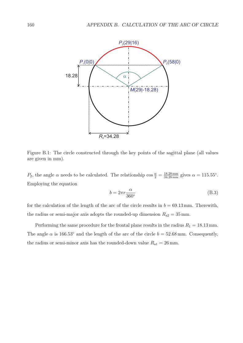
160 APPENDIX B. CALCULATION OF THE ARC OF CIRCLE
P1(0|0) P2(58|0)
P3(29|16)
M(29|-18.28)
R2=34.28
18.28 a
Figure B.1: The circle constructed through the key points of the sagittal plane (all valuesare given in mm).
P2, the angle α needs to be calculated. The relationship cos α2= 18.28mm
34.28mmgives α = 115.55◦.
Employing the equation
b = 2πrα
360◦(B.3)
for the calculation of the length of the arc of the circle results in b = 69.13mm. Therewith,
the radius or semi-major axis adopts the rounded-up dimension Ra2 = 35mm.
Performing the same procedure for the frontal plane results in the radius R1 = 18.13mm.
The angle α is 166.53◦ and the length of the arc of the circle b = 52.68mm. Consequently,
the radius or semi-minor axis has the rounded-down value Ra1 = 26mm.
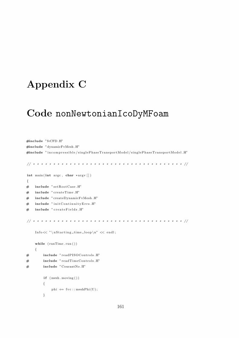
Appendix C
Code nonNewtonianIcoDyMFoam
#include ”fvCFD .H”
#include ”dynamicFvMesh .H”
#include ” incompre s s i b l e / s inglePhaseTransportModel / s inglePhaseTransportModel .H”
// ∗ ∗ ∗ ∗ ∗ ∗ ∗ ∗ ∗ ∗ ∗ ∗ ∗ ∗ ∗ ∗ ∗ ∗ ∗ ∗ ∗ ∗ ∗ ∗ ∗ ∗ ∗ ∗ ∗ ∗ ∗ ∗ ∗ ∗ ∗ ∗ ∗ //
int main ( int argc , char ∗argv [ ] )
{
# include ” setRootCase .H”
# include ” createTime .H”
# include ”createDynamicFvMesh .H”
# include ” i n i tCon t i nu i t yEr r s .H”
# include ” c r e a t eF i e l d s .H”
// ∗ ∗ ∗ ∗ ∗ ∗ ∗ ∗ ∗ ∗ ∗ ∗ ∗ ∗ ∗ ∗ ∗ ∗ ∗ ∗ ∗ ∗ ∗ ∗ ∗ ∗ ∗ ∗ ∗ ∗ ∗ ∗ ∗ ∗ ∗ ∗ ∗ //
Info<< ”\ nStar t ing time loop \n” << endl ;
while ( runTime . run ( ) )
{
# include ” readPISOControls .H”
# include ” readTimeControls .H”
# include ”CourantNo .H”
i f (mesh . moving ( ) )
{
phi += fvc : : meshPhi (U) ;
}
161
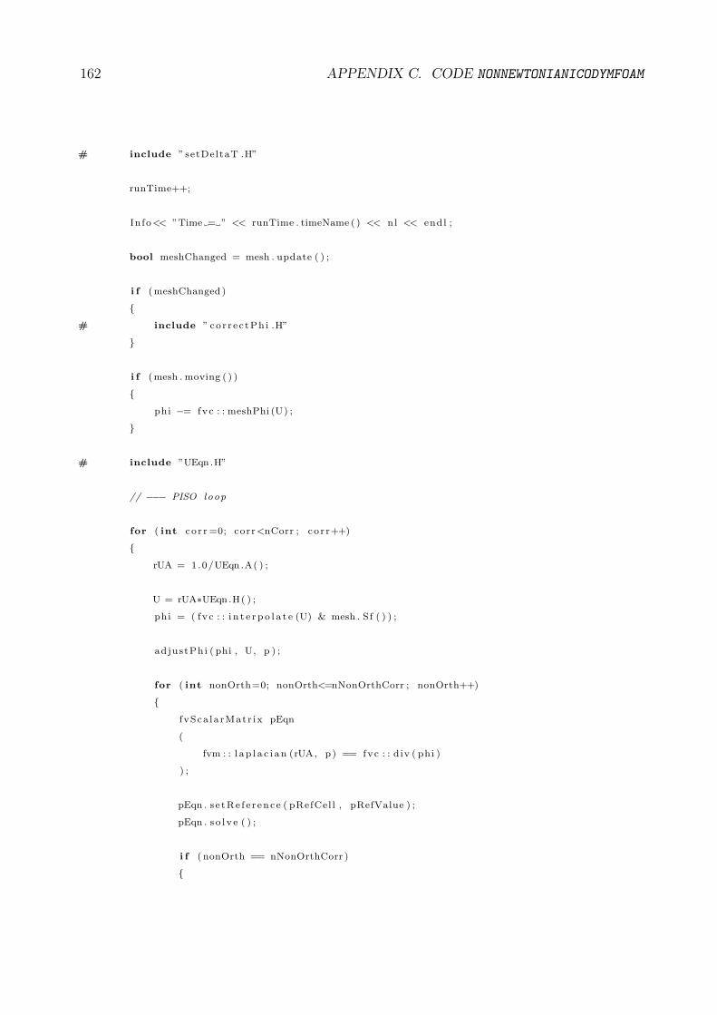
162 APPENDIX C. CODE NONNEWTONIANICODYMFOAM
# include ” setDeltaT .H”
runTime++;
Info<< ”Time = ” << runTime . timeName ( ) << nl << endl ;
bool meshChanged = mesh . update ( ) ;
i f (meshChanged )
{
# include ” co r r e c tPh i .H”
}
i f (mesh . moving ( ) )
{
phi −= fvc : : meshPhi (U) ;
}
# include ”UEqn .H”
// −−− PISO loop
for ( int co r r =0; corr<nCorr ; c o r r++)
{
rUA = 1.0/UEqn .A( ) ;
U = rUA∗UEqn .H( ) ;
phi = ( fvc : : i n t e r p o l a t e (U) & mesh . Sf ( ) ) ;
adjustPhi ( phi , U, p ) ;
for ( int nonOrth=0; nonOrth<=nNonOrthCorr ; nonOrth++)
{
f vSca la rMatr ix pEqn
(
fvm : : l a p l a c i a n (rUA, p) == fvc : : d iv ( phi )
) ;
pEqn . s e tRe f e r ence ( pRefCel l , pRefValue ) ;
pEqn . s o l v e ( ) ;
i f ( nonOrth == nNonOrthCorr )
{
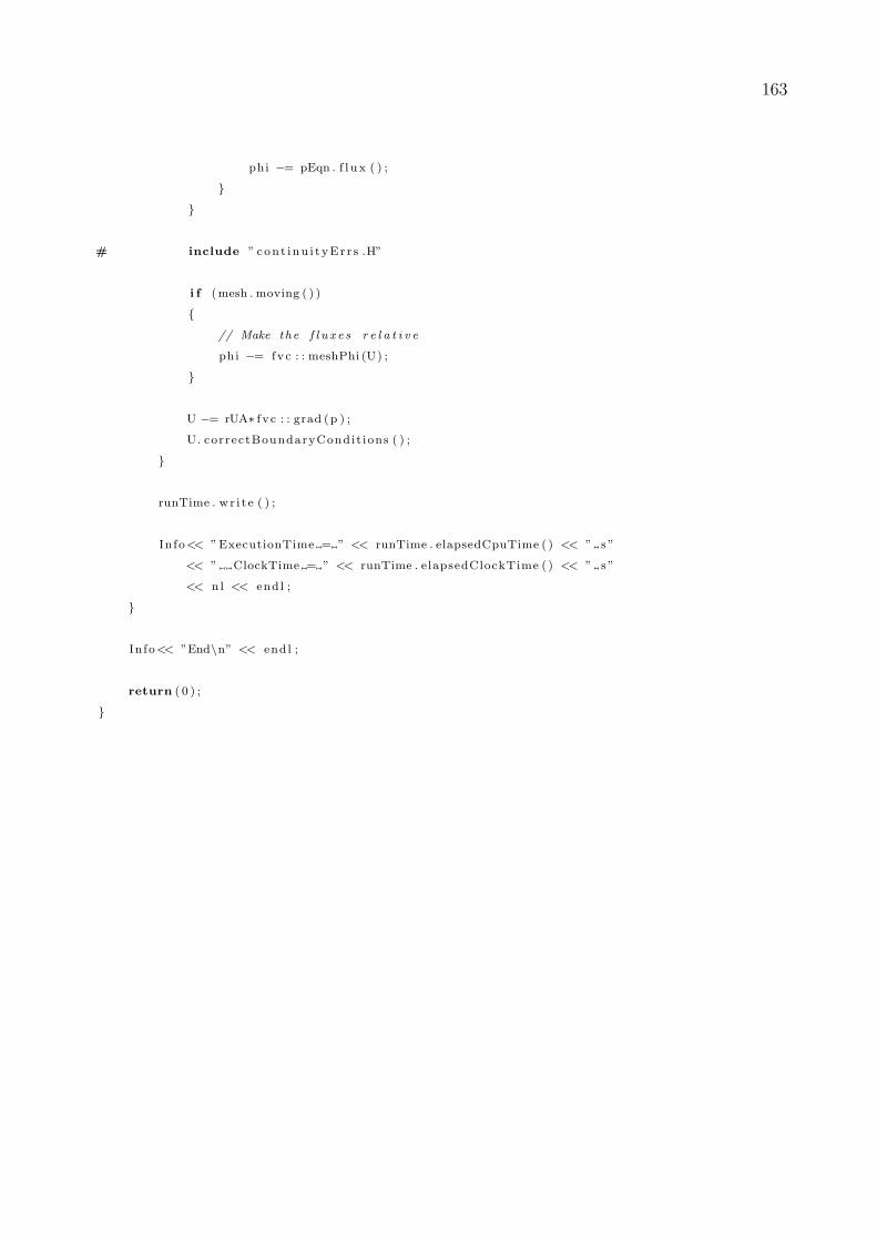
163
phi −= pEqn . f l u x ( ) ;
}
}
# include ” con t inu i t yEr r s .H”
i f (mesh . moving ( ) )
{
// Make the f l u x e s r e l a t i v e
phi −= fvc : : meshPhi (U) ;
}
U −= rUA∗ f v c : : grad (p ) ;
U. correctBoundaryCondit ions ( ) ;
}
runTime . wr i t e ( ) ;
In fo<< ”ExecutionTime = ” << runTime . elapsedCpuTime ( ) << ” s ”
<< ” ClockTime = ” << runTime . elapsedClockTime ( ) << ” s ”
<< nl << endl ;
}
Info<< ”End\n” << endl ;
return ( 0 ) ;
}