University of KentuckyUKnowledge

Theses and Dissertations--Mining Engineering Mining Engineering

2018

INVESTIGATION OF ENVIRONMENTALCADMIUM SOURCES IN EASTERNKENTUCKYElizabeth MaherUniversity of Kentucky, lizziemae26@hotmail.comAuthor ORCID Identifier:

https://orcid.org/0000-0002-7496-5951Digital Object Identifier: https://doi.org/10.13023/ETD.2018.167

Click here to let us know how access to this document benefits you.

This Master's Thesis is brought to you for free and open access by the Mining Engineering at UKnowledge. It has been accepted for inclusion in Thesesand Dissertations--Mining Engineering by an authorized administrator of UKnowledge. For more information, please contactUKnowledge@lsv.uky.edu.

Recommended CitationMaher, Elizabeth, "INVESTIGATION OF ENVIRONMENTAL CADMIUM SOURCES IN EASTERN KENTUCKY" (2018).Theses and Dissertations--Mining Engineering. 41.https://uknowledge.uky.edu/mng_etds/41

STUDENT AGREEMENT:

I represent that my thesis or dissertation and abstract are my original work. Proper attribution has beengiven to all outside sources. I understand that I am solely responsible for obtaining any needed copyrightpermissions. I have obtained needed written permission statement(s) from the owner(s) of each third-party copyrighted matter to be included in my work, allowing electronic distribution (if such use is notpermitted by the fair use doctrine) which will be submitted to UKnowledge as Additional File.

I hereby grant to The University of Kentucky and its agents the irrevocable, non-exclusive, and royalty-free license to archive and make accessible my work in whole or in part in all forms of media, now orhereafter known. I agree that the document mentioned above may be made available immediately forworldwide access unless an embargo applies.

I retain all other ownership rights to the copyright of my work. I also retain the right to use in futureworks (such as articles or books) all or part of my work. I understand that I am free to register thecopyright to my work.

REVIEW, APPROVAL AND ACCEPTANCE

The document mentioned above has been reviewed and accepted by the student’s advisor, on behalf ofthe advisory committee, and by the Director of Graduate Studies (DGS), on behalf of the program; weverify that this is the final, approved version of the student’s thesis including all changes required by theadvisory committee. The undersigned agree to abide by the statements above.

Elizabeth Maher, Student

Dr. Joseph Sottile, Major Professor

Dr. Zacharias Agioutantis, Director of Graduate Studies

INVESTIGATION OF ENVIRONMENTAL CADMIUM SOURCES IN EASTERN KENTUCKY

_____________________________________

THESIS _____________________________________

A thesis submitted in partial fulfillment of the

requirements for the degree of Master of Science in Mining Engineering at the University of Kentucky

By

Elizabeth Maher

Lexington, Kentucky

Director: Dr. Joseph Sottile, Professor of Mining Engineering

Lexington, Kentucky

2018

Copyright © Elizabeth Maher 2018

ABSTRACT OF THESIS

INVESTIGATION OF ENVIRONMENTAL CADMIUM SOURCES IN EASTERN KENTUCKY

Utilizing data collected by the University of Kentucky Lung Cancer Research

Initiative (LCRI), this study investigated potential mining-related sources for the elevated levels of cadmium in Harlan and Letcher counties. Statistical analyses for this study were conducted utilizing SAS. A number of linear regression models and logarithmic models were used to evaluate the significance of the data. The linear regression models consisted of both simple and multivariate types, with the simple models seeking to establish significance between the potential sources and urine cadmium levels and the multivariate models seeking both to identify any statistically significant linear relationships between source types as well as establish a relationship between the potential source and the urine cadmium levels.

The analysis began by investigating which ingestion method caused the increased levels of cadmium exposure, including ingestion through water sources and inhalation of dust. The second step was to analyze a number of sources of dust, particularly those related to mining practices in the area. These included the proximity to the Extended Haul Road System, secondary haul roads, rail roads, and processing plants. Of the variables in the analysis, only the proximity to processing plants showed statistical significance.

KEYWORDS: Mining, Cadmium, Dust, Processing Plants, Transportation

Elizabeth Maher

05/03/2018

INVESTIGATION OF ENVIRONMENTAL CADMIUM SOURCES IN EASTERN KENTUCKY

By

Elizabeth Mae Maher

Dr. Joseph Sottile Director of Thesis

Dr. Zacharias Agioutantis Director of Graduate Studies

04/13/2018

iii

Acknowledgement Statement of support:

This research was supported by the Department of Defense [Congressionally Directed

Medical Research Program, U.S. Army Medical Research and Materiel Command

Program] under award number: 10153006 (W81XWH-11-1-0781). Views and opinions

of, and endorsements by the author(s) do not reflect those of the US Army or the

Department of Defense.

This research was also supported by unrestricted infrastructure funds from the UK Center

for Clinical and Translational Science, NIH grant UL1TR000117.

iv

Contents

Acknowledgement ............................................................................................................. iii

List of Tables ...................................................................................................................... v

List of Figures ....................................................................................................................vi

Section 1: Literature Review .............................................................................................. 1

Section 1.1: Cancer on the National Scope ..................................................................... 1

Section 1.2: Kentucky Cancer Registry Data Collection ................................................ 2

Section 1.3: Previous Studies ......................................................................................... 8

Section 1.4: Current Research ....................................................................................... 12

Section 2: Methodology .................................................................................................... 13

Section 2.1: Information Sources .................................................................................. 13

Section 2.2: Created GIS Data ...................................................................................... 20

Section 3: Discussion ........................................................................................................ 21

Section 3.1: Arsenic Analysis ....................................................................................... 21

Section 3.2: Respiratory vs. Ingestion Through Water ................................................. 22

Section 3.3: Dust Source Analyses ............................................................................... 29

Section 4: Conclusions and Future Work ......................................................................... 36

Section 4.1: Conclusions ............................................................................................... 36

Section 4.2: Future Work .............................................................................................. 38

References ......................................................................................................................... 40

Vita .................................................................................................................................... 43

Table of Contents ............................................................................................................... iv

v

List of Tables

Table 1. Cases and Controls............................................................................................... 5 Table 2. Cadmium Correlation between Zn/Mn .............................................................. 12 Table 3. Sample ANOVA Table ...................................................................................... 18 Table 4. Cadmium vs. Arsenic ANOVA Table ............................................................... 21 Table 5. Well Data ANOVA Table .................................................................................. 22 Table 6. Linear 250 μm < x < 2 mm Dust ANOVA Table ........................................... 23 Table 7. Logarithmic 250 μm < x < 2 mm Dust ANOVA Table..................................... 23 Table 8. Linear 100 μm < x < 250 μm Dust ANOVA Table ........................................... 24 Table 9. Logarithmic 100 μm < x < 250 μm ANOVA Table ........................................ 24 Table 10. Linear 10 μm < x < 100 μm Dust ANOVA Table ....................................... .. 25 Table 11. Logarithmic 10 μm < x < 100 μm Dust ANOVA Table .......................... .......25 Table 12. Linear 2.5 μm < x < 10 μm Dust ANOVA Table .................................... ...... 26 Table 13. Logarithmic 2.5 μm < x < 10 μm Dust ANOVA Table ........................... ...... 26 Table 14. Linear x < 2.5 μm Dust ANOVA Table ..................................................... .... 27 Table 15. Logarithmic s < 2.5 μm Dust ANOVA Table . ............................................. 27 Table 16. Linear Extended Haul Road ANOVA Table ................................................... 29 Table 17. Logarithmic Extended Haul Road ANOVA Table .......................................... 29 Table 18. Linear Secondary Haul Road ANOVA Table ................................................. 30 Table 19. Logarithmic Secondary Haul Road ANOVA Table ........................................ 30 Table 20. Linear Haul Road ANOVA Table ................................................................... 31 Table 21. Logarithmic Haul Road ANOVA Table .......................................................... 31 Table 22. Linear Railroad ANOVA Table ....................................................................... 32 Table 23. Logarithmic Railroad ANOVA Table ............................................................. 32 Table 24. Linear Processing Plant ANOVA Table .......................................................... 34 Table 25. Linear Processing Plant Parameter Estimates .................................................. 34 Table 26. Logarithmic Processing Plant ANOVA Table................................................. 34 Table 27. Logarithmic Processing Plant Parameter Estimates ........................................ 34 Table 28. Multivariate Linear Regression ANOVA Table .............................................. 35 Table 29. Summary Table ................................................................................................ 37

vi

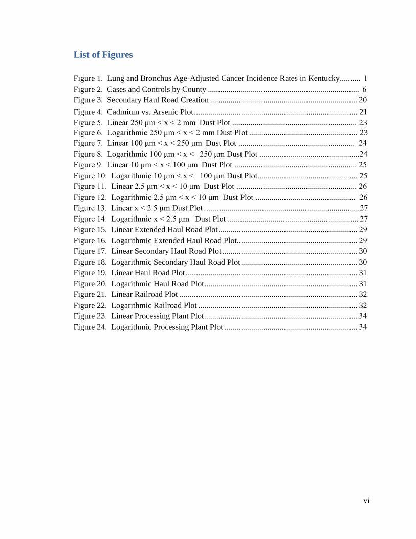
List of Figures

Figure 1. Lung and Bronchus Age-Adjusted Cancer Incidence Rates in Kentucky .......... 1 Figure 2. Cases and Controls by County .......................................................................... 6 Figure 3. Secondary Haul Road Creation ........................................................................ 20 Figure 4. Cadmium vs. Arsenic Plot ................................................................................ 21 Figure 5. Linear 250 μm < x < 2 mm Dust Plot ............................................................. 23 Figure 6. Logarithmic 250 μm < x < 2 mm Dust Plot ..................................................... 23 Figure 7. Linear 100 μm < x < 250 μm Dust Plot ......................................................... 24 Figure 8. Logarithmic 100 μm < x < 250 μm Dust Plot .................................................24 Figure 9. Linear 10 μm < x < 100 μm Dust Plot ............................................................ 25 Figure 10. Logarithmic 10 μm < x < 100 μm Dust Plot................................................. 25 Figure 11. Linear 2.5 μm < x < 10 μm Dust Plot ........................................................... 26 Figure 12. Logarithmic 2.5 μm < x < 10 μm Dust Plot ................................................. 26 Figure 13. Linear x < 2.5 μm Dust Plot . ...........................................................................27 Figure 14. Logarithmic x < 2.5 μm Dust Plot ................................................................ 27 Figure 15. Linear Extended Haul Road Plot .................................................................... 29 Figure 16. Logarithmic Extended Haul Road Plot ........................................................... 29 Figure 17. Linear Secondary Haul Road Plot .................................................................. 30 Figure 18. Logarithmic Secondary Haul Road Plot ......................................................... 30 Figure 19. Linear Haul Road Plot .................................................................................... 31 Figure 20. Logarithmic Haul Road Plot ........................................................................... 31 Figure 21. Linear Railroad Plot ....................................................................................... 32 Figure 22. Logarithmic Railroad Plot .............................................................................. 32 Figure 23. Linear Processing Plant Plot ........................................................................... 34 Figure 24. Logarithmic Processing Plant Plot ................................................................. 34

Section 1: Literature Review

Section 1.1: Cancer on the National Scope

Cancer is the second most common cause of death in the United States and

accounts for twenty percent of the deaths annually in the U.S. (CDC 2017a). With no

absolute cure, over 100 billion dollars is spent annually on the treatment of cancer in the

United States (NIH 2011). “Lung cancer is the leading cause of cancer death and the

second most common cancer among both men and women in the United States” (CDC

2017b). Figure 1 is produced by the Kentucky Cancer Registry (KCR 2017), and depicts

the incidence rates of lung cancer within the state of Kentucky on a county level. This

figure shows an alarming incidence rate of lung cancer in individuals living in

southeastern Kentucky.

Figure 1. Lung and Bronchus Age-Adjusted Cancer Incidence Rates in Kentucky

1

Lung cancer is the “the most common cause of cancer death in Kentucky (KCC

2013).” The state possesses the highest fatality and incidence rates in the country, with

these rates being 69.5 and 94.3 people per 100,000, respectively (CDC 2016a).

Furthermore, every county in Kentucky has a higher incidence rate than the national

average of 62.4 (NIH 2017). Due to the high prevalence of lung cancer in Kentucky, a

large focus of the Center for Disease Control is to determine how to prevent and treat the

potential and current cases in the state.

Section 1.2: Kentucky Cancer Registry Data Collection

In order to study this incidence rate, toenail, hair, dust, and urine samples were

taken from 520 people within Kentucky’s 5th Congressional District. The people within

this study were selected from the list of recently diagnosed individuals from the

Kentucky Cancer Registry. The diagnosed individuals were contacted and asked to

consent to the use of their information for the study. After 150 people with lung cancer

consented to the study, controls were selected on an approximately 2:1 ratio, totaling 370

controls, i.e., individuals diagnosed with cancer, but not lung cancer.

Qualifying Lung Cancers

Qualifying cancers for this study include the subset of cancers located within the

lung. Of those with qualifying cancer types, the cancers were organized by their

topography, histology, and stage.

2

Topography of Cancer

The topography classifications include upper lobe, middle lobe, lower lobe,

overlapping, and not otherwise specified. There are three lobes on the right side of the

lung (upper, middle, and lower) and two lobes on the left side of the lung (upper and

lower) (ACS 2016). Where cancer is seen in the lung is at times indicative of the

contaminant that causes the cancer. This can be seen when looking at the location of

cancers with heavy materials, such as asbestos. However, many contaminants are known

to cause cancer throughout the lung as well. Since the determining method of

contamination is the purpose of the study, and, therefore, unknown, we are under the

assumption that the topography of the cancer is not a useful analyte for this study

(Sanderson, W. personal communication).

Histology of Cancer

The histology of the cancers analyzed throughout this study includes a number of

different cancer types. For the purpose of this analysis, these will be broken down into

small cell carcinoma, large cell carcinoma, adenocarcinoma, squamous cell carcinoma,

neuroendocrine carcinoma, and papillary carcinoma.

Small cell and large cell carcinomas are defined by the size of the affected cells

compared with the size of normal lung cells. Thus, if affected cells are smaller than

normal lung cells, the carcinoma is classified as small cell. Conversely, if affected cells

are larger than normal lung cells, the carcinoma is classified as large cell. Large cell

carcinoma can be divided into a number of different categories based on the appearance

of the lung cancer cells and the cells that they affect.

3

Adenocarcinoma is the cancer originating in the structural cells of the lung. In

contrast, squamous cell carcinoma defines cancer originating in cells located within the

lining of the lung, specifically squamous cells. Neuroendocrine carcinoma refers to those

cancers found in the hormone producing cells of the body, bronchoalveolar carcinoma is

that found in the bronchioles or alveoli, and mucin-producing adenocarcinoma is that

found in the cells that produce mucus for the body.

Another factor utilized in the classification of lung cancer is the shape of the

affected cells; papillary adenocarcinoma refers to cancers in which the afflicted cells

form abnormally shaped cells known as papillary cells. The last classification to address

is the adenosquamous cancer, which is attributed to cases possessing a combination of

adenocarcinoma and squamous cell carcinoma (Sanderson, W. personal communication).

The type of cancer that develops and specific contaminant exposure causing the

cancer are theorized to have a connection; however, there is no distinct research into the

effect of cadmium on the different types of cancer. Therefore, during this study, the

cancer type will not be a factor for analysis (Sanderson, W. personal communication).

Stage of Cancer

The stage of cancer describes the severity of the cancer at the time of detection

and is therefore, highly significant in the determination of proper treatment. Cancer

attributed to stage one is early in development, typically small, and has not spread into

the other parts of the body. Stage Two cancers are typically larger compared to those of

stage one but remain isolated from other regions of the body. If stage two cancers have

spread, typically only the surrounding lymph nodes are affected. Stage three cancer

means that the cancer has started invading the surrounding tissues and is much larger than

4

either stage one or stage two cancers. The most severe cancer stage is Stage Four, where

the cancer has metastasized throughout the entire body, including regions distal to the

cancer’s origin site. In most cases, Stage Four Cancer is fatal (CRU 2017).

Case or Control Status

This study is a single blind study where the analyst for the study was not informed

of the status of the individuals. The study contained 370 controls, which did not have

lung cancer, but underwent the same tests as those with lung cancer. The study also

included 150 cases that did have lung cancer. In order to take a closer look at these data,

the study area was reduced from the original region to include only two counties: Harlan

and Letcher. These two counties had a combined total of 49 case and control points.

Table 1 displays the number of cases and controls contained in the two counties. Three

of the points did not have corresponding GPS coordinates; therefore, the total observation

count is 46 data points.

Table 1. Cases and Controls

Harlan Letcher Case 7 0

Control 18 24

The case and control status of each person in the study was not known to the

researcher at the time the analyses were conducted. The determination of the counties

chosen was based on an overview map of the cases and controls as shown in Figure 2.

5

Figure 2. Cases and Controls by County

Demographic Information and Prior Cancer Status

During the study, a variety of demographical information was collected for further

analysis. These demographics include the participant’s gender, age, BMI, race, marital

status, education, income, health coverage, and county of residence. In addition, the

study specifies only individuals previously registered with the Kentucky Cancer Registry.

Smoking Questionnaire Data

The Kentucky Cancer Registry had all participants answer a number of questions

based on each individual’s past and present smoking practices. The questionnaire

includes the smoking of cigarettes, cigars, pipes, marijuana, and other smoking methods.

Examples of the questions asked include the age smoking began and if the participant

tried to quit. Data collected via the questionnaire were compared with the participants’

hair nicotine levels for informal validation of their responses, as described in the next

section.

6

Validated Data

The numerical data collected for the study includes toenail, soil, water, and urine

samples, as well as GPS coordinates. These data sets were analyzed for the following

analytes:

• Aluminum (Al)

• Chromium (Cr)

• Manganese (Mn)

• Iron (Fe) (All Except Soil

Data)

• Cobalt (Co)

• Nickel (Ni)

• Copper (Cu)

• Zinc (Zn)

• Arsenic (As)

• Selenium (Se)

• Cadmium (Cd)

• Lead (Pb)

• Uranium (U)

The elements studied in this analysis are hazardous to the human body when

ingested. The ingestion of these materials can be achieved via dust inhalation, food

consumption, liquid consumption, and skin contact. The ingestion method and level of

carcinogenicity vary greatly on the analyte. The nail and urine samples were used to

determine the long-term and short-term exposures of the individuals while the water and

soil analyses were used to aid in quantifying possible levels of environmental exposures.

The study also included the collection of hair samples. The hair samples are meant to

determine the nicotine level of each participant, and thus determine the how much the

participant smokes. This information was used to mitigate potential response bias

inherently present in a questionnaire-based study by comparing answers with the

individual’s hair nicotine levels. The GPS coordinates collected during the study include

the latitude and longitude of each individual’s residence.

7

Questionnaire Data

The questionnaire answered by each member of the study includes family history,

health, occupation, physical activity, and residential history. The family history of the

participant includes all cancers known to have occurred in the past, with lung cancer

being isolated as the focus and all other cancers being grouped together. The

participants’ family members include mother, father, sister, brother, daughter, and son.

The health data collected in the questionnaire include various lifestyle questions

pertaining to sleep time and perceived energy level. These questions intend to identify

the level of the stress and activity of the participants. In addition, data concerning levels

of daily physical activity were collected with activity being classified as strenuous,

moderate, and mild. This information was used as a measure of fitness. The occupational

information of each participant was also collected to determine what potential

occupational exposures might exist. Furthermore, residential history was collected to

determine the levels of exposure that may be experienced by each participant based upon

the environment in which they live.

Section 1.3: Previous Studies

Most of the lung cancer cases in the United States, i.e., 80-90%, are attributed to

cigarette smoking (CDC 2016c). While smoking is the predominant cause of lung

cancer, there are still over 10,000 lung cancer fatalities per 100,000 due to other sources.

Kentucky has the highest rate of smoking in the United States with 28.3% of Kentuckians

being current smokers (KCC 2013). Because of this, the first hypothesis tested with this

data determined if the high lung cancer incidence rate was simply a product of the high

smoking rate in the area. The hair samples were used to determine the level of nicotine

8

in the individuals’ system. This analysis was conducted by Dr. Nancy Johnson and Ms.

Ellen Flora at the University of Kentucky. The conclusions show that there is

insignificant correlation between smoking rates and cadmium levels to establish that

smoking is the sole cause of the high cancer rates observed in eastern Kentucky.

However, because there is an extremely high rate of smoking throughout the

region, the effect of smoking should be adjusted for subsequent analyses. The high

cadmium subset includes 179 of the 520 case and control subjects. In this case, high

cadmium is defined as those individuals with cadmium exposure levels above the ACGIH

(American Conference of Governmental Industrial Hygienists) suggested limit. Using

this subset, the researchers determined that “[only] the correlation between smokers with

high Cd is statistically significant (Flora 2017).” This significant correlation is only

present in this subset of the data, rather than throughout the entire data set. This analysis

suggests a possible synergistic effect between cadmium exposure and smoking since the

cadmium levels only showed correlation within the high cadmium subgroup (Flora 2017).

Dr. Johnson also conducted analysis comparing the urine samples to the case-

control status of the individual. Based on the statistical analysis, it was concluded that

the case or control status of an individual correlated with the level of cadmium in their

urine. This means that the cases are more likely to have a high cadmium level and the

controls are likely not to be contained in the high cadmium subset.

In a study conducted by Li, et. al., they concluded that “cadmium, [copper], and

[lead] from anthropogenic source[s] were mainly found at mine entrance road sides and

in sites closest to coal mines (Li, et al. 2017).” The same study concluded that the “total

carcinogenic risk was mainly contributed by Cd and Ni (Li, et. al. 2017).”

9

Since cadmium is known to be a carcinogen with effect on the respiratory system,

correlations of other elements to cadmium were conducted and it was concluded that Zinc

and Manganese in urine each showed a high level of correlation with the elevated

cadmium levels for both, the overall urine values, and the high cadmium subset.

Table 2. Cadmium Correlation between Zn/Mn

All Urine High Cadmium Subset

Urine Manganese

Urine Zinc Urine

Manganese Urine Zinc

Coefficient 0.59780 0.26244 Coefficient 0.31125 0.20141 p-value <0.0001 <0.0001 p-value <0.0001 0.0069

Sample size 520 520 Sample size 179 179

These results, shown in Table 2, demonstrate that the level of Zinc and

Manganese were highly correlated to the levels of Cadmium in urine. Based on current

cancer research, compiled by ACGIH, both Manganese and Zinc have insufficient

evidence to show causation of lung cancer (ACGIH 2015). Due to this, it was concluded

that cadmium was the contaminant that should be the focus of subsequent analyses.

Upon analyzing the correlation between the different elements tested, it was also

determined that Arsenic showed a possible correlation with cadmium, therefore Arsenic

was a secondary analyte for this study.

Cadmium is classified as a type A2 carcinogen. This classification means that it

is a “suspected human carcinogen” according to the (ACGIH) book (ACGIH 2015).

Cadmium is a naturally occurring element that can enter the body in a number of ways.

Cadmium is typically found in zinc, lead, and carbonate ores. While cadmium is

naturally occurring, it does not break down once it is on ground surface level. It can be

found in the air through the breakdown of rock and once deposited; it stays in the system

of the plants and animals that absorb it. The exposure most humans have to cadmium is 10

through ingesting food, inhalation, or ingestion through water. Analysis was conducted

on the water sources of the homes of the study group. The results of this analysis

showed that tap water was not the source of cadmium contamination.

One of the main sources of cadmium exposure throughout the country is tobacco

cigarette smoking, which is why the cadmium levels present due to cigarettes must be

accounted for in subsequent studies. In addition to lung cancer, cadmium is found to

cause cancer in the prostate as well as a low possibility of cancer in the pancreas, kidney,

renal cell, bladder, breast and endometrium (IARC 2013). “Exposure to cadmium

particulates leads to cadmium absorption in animals and humans”; however, the rate of

absorption is extremely low. When it is absorbed, it causes damage to the tubular cells

and is excreted very slowly (IARC 2013). There is limited data on the effect of cadmium

in humans, though animal research suggests that cadmium causes cancer through

induction of oxidative stress, inhibition of DNA repair, and deregulation of cell

proliferation and disturbance of tumor-suppressor functions.

The Agency for Toxic Substances and Disease Registry (ATSDR) provides a

comprehensive study of the use of urine for the analysis of cadmium exposure:

“With low to moderate chronic exposure, urinary cadmium reflects integrated

exposure over time and total body burden (Jarup, 2002). According to the

National Health and Nutrition Examination Survey (NHANES) data, healthy

young non-exposed, nonsmokers in the United States have very low levels of

urinary cadmium (average cadmium level of 0.08 µg/g creatinine; levels increase

with age to 0.26 µg/gm of creatinine). “The Third National Report on Human

Exposure to Environmental Chemicals" showed that during 2001- 2002 the

11

geometric means for adults aged 20 and older was 0.210µg/gm creatinine (CDC

2005) (ATSDR 2008).”

In a study conducted by Nancy Johnson, the cadmium levels for the overall study

group correlate with the age of the participants; however, the cadmium levels do not

correlate for the high cadmium subgroup. This means that the elevated levels of

cadmium exposure do not depend on the age of the participant as it should if the

cadmium exposure was consistent through time.

Section 1.4: Current Research

Current research focused on the determining the sources of cadmium exposure.

One type of analysis is to look at the ‘valleyness factor’ of the living location of each

resident. This intends to look at how far into the valley the individual lives as well as

taking into account how steep the nearby slopes are. Another study is to consider

whether or not the individual maintains a garden and whether there is run off from the

roads entering the water supply to the garden. Another study looks at the occupational

history of those within the study group and determines if they have a correlation to the

data. An additional study focuses on the proximity of the house to the closest road.

Coal mining is the major industry throughout the study region. With this

in mind, it is crucial to determine if the exposure is due to the environment of the

industry. Analyses of the coal layers within the region were used to determine if the coal

dust was a source of cadmium; however, the levels of cadmium in the coal bed are very

low (Eble, C. personal communication). The levels of cadmium in the surrounding rock

layers have not been determined. The possibility that an individual worked in the

industry was not adjusted for in the data and is part of a separate occupational study.

12

Section 2: Methodology

Section 2.1: Information Sources

Lung Cancer Research Initiative Data

The Lung Cancer Research Initiative (LCRI) provided the data used for this

study, including the urine and nail cadmium levels, GPS coordinates, and urine arsenic

values. The cadmium levels utilized for this study do not contain the adjustment for the

smoking levels of the participants. This means that any data variability will be under

represented since there is a known presence of smoking in the area.

Creatinine correction procedures were utilized to validate the data being used.

“Correction to creatinine excretion would seem most appropriate in routine biological

monitoring. Manganese, cadmium, and hippuric acid are candidates for this approach

(WHO, 1996). Creatinine correction values are obtained by the following adjustment:

𝐶𝐶𝐶𝐶𝑚𝑚_𝑐𝑐𝑐𝑐𝑐𝑐𝑐𝑐 =𝐶𝐶𝐶𝐶𝑣𝑣_𝑐𝑐𝑐𝑐𝑐𝑐𝑐𝑐

𝐶𝐶𝐶𝐶𝐶𝐶𝑐𝑐𝑐𝑐𝑐𝑐𝑐𝑐

Where,

𝐶𝐶𝐶𝐶𝑚𝑚_𝑐𝑐𝑐𝑐𝑐𝑐𝑐𝑐 = corrected mass concentration of Cadmium, 𝜇𝜇𝜇𝜇𝜇𝜇

,

𝐶𝐶𝐶𝐶𝑣𝑣_𝑐𝑐𝑐𝑐𝑐𝑐𝑐𝑐 = Cadmium concentration in urine, 𝜇𝜇𝜇𝜇𝐿𝐿

𝐶𝐶𝐶𝐶𝐶𝐶𝑐𝑐𝑐𝑐𝑐𝑐𝑐𝑐 = Creatinine concentration in urine, 𝜇𝜇𝐿𝐿

13

This correction allows researchers to take into account the volume of urine

collected, thereby mitigating error for dilution. According to the World Health

Organization (WHO), “When the urine is very dilute (urinary creatinine < 0.3 g/L) or

concentrated (urinary creatinine > 3.0 g/L) it is unlikely that any correction will give

accurate results (WHO, 1996).” After the creatinine corrections were completed, one

sample was eliminated for a creatinine level below 0.3 g/L and two others were

eliminated because the creatinine levels were above 3.0 g/L to follow the WHO

recommendation.

Road Data

The road data utilized during this study includes local, county, state, and interstate

routes in the study area. The road data was obtained from the Kentucky Geological

Survey because the KGS keeps detailed road data in a useful format.

Railroads

The railroad data was also provided by the KGS, which keeps records of the

railroads present throughout the state and marks them as active or inactive (historic).

This study looks at the railroads present during all stages of time, so both sets of railroad

data were combined into a single data set for this analysis.

14

Extended Haul Roads

The Extended Haul Roads were provided by the Kentucky Transportation Center

(KTC) at the University of Kentucky. Extended Haul Roads are defined as those that

“exceed normal weight limits through the payment of an annual decal fee (Pigman, et. al.,

1995)”. These roads “carry over 50,000 tons of coal in a calendar year,” making them

extremely important to the survival of the coal industry in Eastern Kentucky (Pigman, et.

al., 1995). With the knowledge that these roads carry extremely high levels of coal

traffic, it was important to conduct an analysis of these transportation routes.

Permitted Haul Roads

The permitted haul roads are those created by a mining company to transport coal

within the limits of the mine site. These roads were determined using the data collected

by Kentucky Geological Survey from mine permit applications. The permitted haul

roads include all of the roads permitted for construction. Note that in some cases, a road

permitted for construction may not have been constructed by the mining company, and

there are no records of indicating which permitted haul roads were constructed. For this

research, all permitted haul roads were included.

Well Data

The well water data was collected by members of the Kentucky Geological

Survey. The Kentucky Geological Survey keeps a record of the chemical levels measured

within the wells throughout the state. The study utilizes both, the levels of cadmium

measured within the wells, and the GPS coordinates of the well.

15

Processing Plant Data

The processing plants within this study came from two different sources. The

first is the University of Kentucky Mining Engineering Department and the second is the

Kentucky Geological Survey. Both data sets contain the GPS coordinates of the

processing plants as well as the company name of the mine. Both of the data sets were

combined to create a more complete image of the processing plants within the region,

however, they did not show much overlap, so it is likely that the current analysis does not

contain a complete processing plant data set.

Statistical Analysis

The statistical analyses of this study were conducted using SAS. SAS

(previously, Statistical Analysis System) was developed by North Carolina State

University from 1966-1976, when the SAS Institute was incorporated. The SAS software

Suite has been developed for advanced analytics, multivariate analyses, predictive

analytics, data management, and business intelligence. For this research, the analyses

consist of simple linear regression models and multivariate regression models depending

on the type of analysis desired and determine if there is a possible relationship between

the variables in the analysis. For the logarithmic models of the data, the logarithmic

values were computed and used as a new variable in the subsequent linear analysis. For

these equations, y refers to the dependent variable, x refers to the regressor (independent)

variable, a refers to the y-intercept and b refers to the correlation coefficient.

The simple linear regression analyses create the summary equation:

𝑦𝑦 = 𝑎𝑎 + 𝑏𝑏𝑏𝑏

16

Multivariate linear regression analyses create the summary equation:

𝑦𝑦 = 𝑎𝑎 + 𝑏𝑏1𝑏𝑏1 + ⋯+ 𝑏𝑏𝑐𝑐𝑏𝑏𝑐𝑐

For the purpose of this study, three parameters are used to determine the adequacy

of the regression model and significant factors: the p-value, the adjusted 𝐶𝐶2 value, and the

model coefficient(s).

Regression analysis is used to produce an equation that describes the relationship

between one or more regressor variables and the response variable. A hypothesis test is

used to determine if the coefficient for each term in the regression equation is equal to

zero, i.e., that a particular regressor has no significant effect on the response. For this

analysis, the null hypothesis is that the coefficient is equal to zero. The alternative

hypothesis is that the coefficient is not equal to zero, i.e., that a particular regressor does

affect the response.

Determination of the probability of a Type I error is used to test for significance.

The probability of a Type I error is the probability of incorrectly rejecting the null

hypothesis, or colloquially, falsely inferring the existence of something that is not

present. In the case of regression analysis, it is inferring the existence of a non-zero

coefficient when the true coefficient is zero. Therefore, it is necessary for the individual

conducting the analysis to select the probability of a Type I error to be sufficiently small

such that there is a high level of confidence in concluding that a particular coefficient is

non-zero. Typical values selected for the probability of a Type I error are 0.01, 0.05, and

0.10. The Greek letter α is commonly used to represent the probability of a Type I error.

17

The p-value approach is commonly used to determine statistical significance in

regression analysis. The desired level for the probability of a Type I error (the p-value) is

selected before analysis is conducted, and if the probability of a Type I error (α) is less

than the p-value, the null hypothesis is rejected and the coefficient is considered to be

significant. Although the selection of an appropriate p-value is somewhat arbitrary, most

statisticians select a p-value of 0.05. Therefore, for this research, a p-value of 0.05 was

used in all analyses.

The analysis of the p-value utilized an Analysis of Variance (ANOVA) table. An

example of the ANOVA table format used for subsequent analyses is shown below:

Table 3. Sample ANOVA Table

Source DF Sum of Squares Mean Squares F value Pr>F Model k-1 SSM SST/(k-1) MSM/MSE Error N-k SSE SSE/(N-k)

Corrected Total N-1 SST

Where,

𝐷𝐷𝐷𝐷 = 𝐶𝐶𝐶𝐶𝑑𝑑𝐶𝐶𝐶𝐶𝐶𝐶𝑑𝑑 𝑜𝑜𝑜𝑜 𝑜𝑜𝐶𝐶𝐶𝐶𝐶𝐶𝐶𝐶𝑜𝑜𝑓𝑓

𝑘𝑘 = 𝑛𝑛𝑛𝑛𝑓𝑓𝑏𝑏𝐶𝐶𝐶𝐶 𝑜𝑜𝑜𝑜 𝑣𝑣𝑎𝑎𝐶𝐶𝑣𝑣𝑎𝑎𝑏𝑏𝑣𝑣𝐶𝐶𝑑𝑑 𝑣𝑣𝑛𝑛 𝑎𝑎𝑛𝑛𝑎𝑎𝑣𝑣𝑦𝑦𝑑𝑑𝑣𝑣𝑑𝑑 𝑁𝑁 =

𝑇𝑇ℎ𝐶𝐶 𝑛𝑛𝑛𝑛𝑓𝑓𝑏𝑏𝐶𝐶𝐶𝐶 𝑜𝑜𝑜𝑜 𝑑𝑑𝑎𝑎𝑓𝑓𝑠𝑠𝑣𝑣𝐶𝐶𝑑𝑑 𝑜𝑜𝑜𝑜 𝐶𝐶𝑎𝑎𝑒𝑒ℎ 𝑣𝑣𝑎𝑎𝐶𝐶𝑣𝑣𝑎𝑎𝑏𝑏𝑣𝑣𝐶𝐶 𝑠𝑠𝐶𝐶𝐶𝐶𝑑𝑑𝐶𝐶𝑛𝑛𝑝𝑝

𝑆𝑆𝑆𝑆𝑆𝑆 = 𝑆𝑆𝑛𝑛𝑓𝑓 𝑜𝑜𝑜𝑜 𝑆𝑆𝑆𝑆𝑛𝑛𝑎𝑎𝐶𝐶𝐶𝐶𝑑𝑑 𝑜𝑜𝑜𝑜𝐶𝐶 𝑝𝑝ℎ𝐶𝐶 𝑆𝑆𝑜𝑜𝐶𝐶𝐶𝐶𝑣𝑣

𝑆𝑆𝑆𝑆𝑆𝑆 = 𝑆𝑆𝑛𝑛𝑓𝑓 𝑜𝑜𝑜𝑜 𝑆𝑆𝑆𝑆𝑛𝑛𝑎𝑎𝐶𝐶𝐶𝐶𝑑𝑑 𝑜𝑜𝑜𝑜𝐶𝐶 𝑝𝑝ℎ𝐶𝐶 𝑆𝑆𝐶𝐶𝐶𝐶𝑜𝑜𝐶𝐶

𝑆𝑆𝑆𝑆𝑇𝑇 = 𝑇𝑇𝑜𝑜𝑝𝑝𝑎𝑎𝑣𝑣 𝑆𝑆𝑛𝑛𝑓𝑓 𝑜𝑜𝑜𝑜 𝑆𝑆𝑆𝑆𝑛𝑛𝑎𝑎𝐶𝐶𝐶𝐶𝑑𝑑

𝑆𝑆𝑆𝑆𝑆𝑆 = 𝑆𝑆𝐶𝐶𝑎𝑎𝑛𝑛 𝑆𝑆𝑆𝑆𝑛𝑛𝑎𝑎𝐶𝐶𝐶𝐶𝑑𝑑 𝐷𝐷𝑜𝑜𝐶𝐶 𝑝𝑝ℎ𝐶𝐶 𝑆𝑆𝑜𝑜𝐶𝐶𝐶𝐶𝑣𝑣

𝑆𝑆𝑆𝑆𝑆𝑆 = 𝑆𝑆𝐶𝐶𝑎𝑎𝑛𝑛 𝑆𝑆𝑆𝑆𝑛𝑛𝑎𝑎𝐶𝐶𝐶𝐶𝑑𝑑 𝑜𝑜𝑜𝑜𝐶𝐶 𝑝𝑝ℎ𝐶𝐶 𝑆𝑆𝐶𝐶𝐶𝐶𝑜𝑜𝐶𝐶

𝐷𝐷 = 𝐷𝐷 − 𝑑𝑑𝑝𝑝𝑎𝑎𝑝𝑝𝑣𝑣𝑑𝑑𝑝𝑝𝑣𝑣𝑒𝑒

18

The Sum of Squares for the model, error, and total are determined using:

�(𝑏𝑏 − �̅�𝑏)2

Where,

𝑏𝑏 = 𝑑𝑑𝑎𝑎𝑓𝑓𝑠𝑠𝑣𝑣𝐶𝐶 𝑣𝑣𝑎𝑎𝑣𝑣𝑛𝑛𝐶𝐶

�̅�𝑏 = 𝑑𝑑𝑎𝑎𝑓𝑓𝑠𝑠𝑣𝑣𝐶𝐶 𝑓𝑓𝐶𝐶𝑎𝑎𝑛𝑛

By adding the variability up for each of the samples in the set, the variance

present in the entire set is determined and the subsequently divided by the number of

degrees of freedom. This allows for the determination of the F-statistic. The F-statistic is

a measure of the ratio of the variation between the sample means to the variation within

the samples. The p-value is determined using the F-statistic and the degrees of freedom.

In all subsequent analyses, 𝑃𝑃𝐶𝐶 > 𝐷𝐷 denotes the p-value present.

In simple linear regression analysis, the coefficient of determination (𝐶𝐶2) is used

to ascertain how well the data fit the model. In particular, the coefficient of

determination refers to the amount of variability that the model explains. In multivariate

regression, the coefficient of multiple determination (also 𝐶𝐶2) is used to determine how

well the data fit the regression model. Below is the equation for the 𝐶𝐶2value:

𝐶𝐶2 =(𝑛𝑛(∑𝑏𝑏𝑦𝑦) − (∑𝑏𝑏)(∑𝑦𝑦))2

[(𝑛𝑛(∑𝑏𝑏2)) − (∑𝑏𝑏)2][(𝑛𝑛(∑𝑦𝑦2)) − (∑𝑦𝑦)2]

The adjusted 𝐶𝐶2 value differs from is by adjusting the value for the number of variables

considered in the analysis. The final reporting within the analysis is the final equation

generated by the regression analysis.

19

Section 2.2: Created GIS Data

Secondary Haul Roads

Secondary Haul Roads were identified utilizing the overall road data, the

permitted haul roads, and the Extended Haul Roads. The concept was to connect the two

haul road data types together using the roads recorded by all road data. This would

identify the most likely routes from each mine site to the highest-trafficked coal roads in

the region. The aim of this analysis was to determine if the dust from the transportation of

the coal was contributing to the high cadmium levels and increased rate of lung cancer in

the study area. This procedure is shown in Figure 3, with the extended haul roads

denoted in black and the permitted haul roads in green and all roads shown in yellow.

Those roads flagged as secondary haul roads are those (in purple) where, as the figure

shows, the permitted haul roads link directly to a main road, which can be followed to the

nearest extended haul road in the vicinity.

Figure 3. Secondary Haul Road Creation

20

Section 3: Discussion

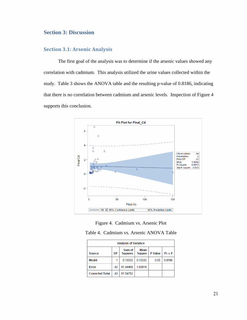
Section 3.1: Arsenic Analysis

The first goal of the analysis was to determine if the arsenic values showed any

correlation with cadmium. This analysis utilized the urine values collected within the

study. Table 3 shows the ANOVA table and the resulting p-value of 0.8186, indicating

that there is no correlation between cadmium and arsenic levels. Inspection of Figure 4

supports this conclusion.

Figure 4. Cadmium vs. Arsenic Plot

Table 4. Cadmium vs. Arsenic ANOVA Table

21

Section 3.2: Respiratory vs. Ingestion Through Water

The second goal of this analysis was to determine whether the method of

exposure was through airborne particles or through waterborne particles. In order to

determine this, the cadmium levels within the urine were compared both to the cadmium

levels in the dust collected at the house as well as to the cadmium levels within, and the

location of, the nearest well.

Water Sources

Previous analysis has shown that tap water was not a significant source of

cadmium exposure. However, throughout most of the United States, including Eastern

Kentucky, individual houses have transitioned to being supplied via city water rather than

utilizing their own well. Because this is a fairly recent change, the nearby wells were

used to show possible previous cadmium exposures. As shown in Table 4, with a p-value

of 0.5789, the well data shows that when doing a multivariate analysis on the two

variables (levels and distance), there is no significant correlation.

Table 5. Well Data ANOVA Table

22

Respiratory Sources

The respiratory data collected was divided into five different categories based on

particle sizes, with each size fraction analyzed separately.

Linear and Logarithmic Analyses of Size Fraction 250 μm < x < 2 mm

Based on the p-values from the two statistical analyses (0.5532 and 0.3960), we

can conclude that there is no statistically significant relationship between the urine

cadmium levels and the dust cadmium levels within this size fraction.

Linear

Figure 5. Linear 250 μm < x < 2 mm Dust Plot

Table 6. Linear 250 μm < x < 2 mm Dust ANOVA Table

Logarithmic

Figure 6. Logarithmic 250 μm < x < 2 mm Dust Plot

Table 7. Logarithmic 250 μm < x < 2 mm Dust ANOVA Table

23

Linear and Logarithmic Analyses of Size Fraction 100 μm < x < 250 μm

The linear and logarithmic relationships both show no statistical significance with

p-values of 0.4128 and 0.2938, respectively.

Linear

Figure 7. Linear 100 μm < x < 250 μm Dust Plot

Table 8. Linear 100 μm < x < 250 μm Dust ANOVA Table

Logarithmic

Figure 8. Logarithmic 100 μm < x < 250 μm Dust Plot

Table 9. Logarithmic 100 μm < x < 250 μm ANOVA Table

24

Linear and Logarithmic Analyses of Size Fraction 10 μm < x < 100 μm

The p-values obtained through the linear and logarithmic analyses are 0.7015 and

0.4675, respectively. These p-values are much higher than the required value of 0.05, so

the cadmium levels in the dust show no statistically significant relationship with the

cadmium levels found in the urine.

Linear

Figure 9. Linear 10 μm < x < 100 μm Dust Plot

Table 10. Linear 10 μm < x < 100 μm Dust ANOVA Table

Logarithmic

Figure 10. Logarithmic 10 μm < x < 100 μm Dust Plot

Table 11. Logarithmic 10 μm < x < 100 μm Dust ANOVA Table

25

Linear and Logarithmic Analyses of Size Fraction 2.5 μm < x < 10 μm

The p-values found through this analysis are 0.9321 along the linear scale and

0.9247 along the logarithmic scale. Neither of these show a statistically significant

relationship between the variables.

Linear

Figure 11. Linear 2.5 μm < x < 10 μm Dust Plot

Table 12. Linear 2.5 μm < x < 10 μm Dust ANOVA Table

Logarithmic

Figure 12. Logarithmic 2.5 μm < x < 10 μm Dust Plot

Table 13. Logarithmic 2.5 μm < x < 10 μm Dust ANOVA Table

26

Linear and Logarithmic Analyses of Size Fraction x < 2.5 μm

The linear relationship of analysis produced a p-value of 0.4563 while the

logarithmic relationship analysis produces a 0.3451. These p-values are larger than the

required alpha of 0.05, so we conclude that the relationship between the variables is not

statistically significant for both sets.

Linear

Figure 13. Linear x < 2.5 μm Dust Plot

Table 14. Linear x < 2.5 μm Dust ANOVA Table

Logarithmic

Figure 14. Logarithmic x < 2.5 μm Dust Plot

Table 15. Logarithmic s < 2.5 μm Dust ANOVA Table

27

Analysis Discussion of All Size Fractions

None of the p-values shows that there are statistically significant relationships

between the cadmium levels in dust and the cadmium levels in urine. These results are

not indicative of a relationship between the dust and urine cadmium levels; however,

there are only four values for the lowest three size fractions and six values for the highest

two. This means that while the results of the analysis are insignificant, the power of the

results is extremely low. Due to this, it is recommended that additional studies take place

to expand the power of the statistics and provide a more thorough look into the

relationship.

Discussion on the Well Data vs. the Dust Data

Based on the data obtained through the two analyses, it was concluded that

sources of dust should be analyzed for any correlation between proximity to these sources

and the urine cadmium levels measured during the preliminary part of this study. This

conclusion is based on the fact that the power of the well data is so much greater than that

of the dust data. Since there are only a maximum of six observations for the dust, no real

conclusion can be made from this, while conclusions can be made based on the well data

because there are 43 observations. In this study, the sources of dust analyzed include

Extended Haul Roads, secondary haul roads, processing plants, and railroads.

28

Section 3.3: Dust Source Analyses

Linear and Logarithmic Extended Haul Road Analyses

The p-values determined through the Extended Haul Road analysis were 0.7681

and 0.8430 for the linear and logarithmic models, respectively. These p-values indicate

that there is insufficient evidence to conclude that there is any correlation between the

proximity to the Extended Haul Roads and the cadmium levels within the urine.

Linear

Figure 15. Linear Extended Haul Road Plot

Table 16. Linear Extended Haul Road ANOVA Table

Logarithmic

Figure 16. Logarithmic Extended Haul Road Plot

Table 17. Logarithmic Extended Haul Road ANOVA Table

29

Linear and Logarithmic Secondary Haul Road Analyses

The p-values for these analyses are 0.7495 and 0.2172, for the linear and

logarithmic analyses, respectively. These p-values are greater than 0.05, so the

conclusion can be made that there is no interaction between the two variables.

Linear

Figure 17. Linear Secondary Haul Road Plot

Table 18. Linear Secondary Haul Road ANOVA Table

Logarithmic

Figure 18. Logarithmic Secondary Haul Road Plot

Table 19. Logarithmic Secondary Haul Road ANOVA Table

30

Linear and Logarithmic Combined Haul Road Analyses

The p-values from the combined (Extended Haul Roads and secondary haul

roads) lead to the same conclusions as the individual analyses. The p-values are 0.3871

and 0.1186, respectively. This indicates that the increased levels of cadmium in urine are

not due to the transportation of coal along the roadways.

Linear

Figure 19. Linear Haul Road Plot

Table 20. Linear Haul Road ANOVA Table

Logarithmic

Figure 20. Logarithmic Haul Road Plot

Table 21. Logarithmic Haul Road ANOVA Table

31

Linear and Logarithmic Railroad Analyses

The other major transportation method utilized by mining companies throughout

the year is the railroad system. The linear and logarithmic values from the analysis are

0.1181 and 0.0608, respectively. These p-values are relatively low, but still greater than

the required p-value of 0.05. Through this analysis, it is concluded that the railroads do

not have an effect on the cadmium levels in the urine of those living nearby.

Linear

Figure 21. Linear Railroad Plot

Table 22. Linear Railroad ANOVA Table

Logarithmic

Figure 22. Logarithmic Railroad Plot

Table 23. Logarithmic Railroad ANOVA Table

32

Linear and Logarithmic Processing Plant Analysis

The linear and logarithmic p-values of the regression analysis on the processing

plants are 0.0185 and 0.0062, respectively. Both of these analyses return statistically

significant values. The parameter estimate for the linear model is -0.2746, meaning that

for each mile farther from a processing plant one lives, cadmium level decreases by

0.2746. Similarly, when looking at the logarithmic model, the slope is also negative with

a coefficient of -0.11111. The linear model is shown by 𝑣𝑣𝑜𝑜𝑑𝑑10(𝑦𝑦𝐶𝐶𝐶𝐶) = 𝑎𝑎𝑏𝑏 + 𝛽𝛽 where x

represents miles, a represents the coefficient and β represents the intercept of the line.

𝑦𝑦𝐶𝐶𝐶𝐶 = 10𝑎𝑎𝑎𝑎+𝛽𝛽 = 10𝛽𝛽10𝑎𝑎𝑎𝑎

𝑦𝑦𝐶𝐶𝐶𝐶 = 100.0868810−0.11111𝑎𝑎

𝑦𝑦𝐶𝐶𝐶𝐶 = 1.2214 ∗ 10−0.11111𝑎𝑎

From this, it is concluded that the farther one lives from a processing plant, the

lower the level of cadmium in the urine since both of the values show a negative

relationship.

The adjusted 𝐶𝐶2 values are 0.1068 and 0.1487 for the linear and logarithmic

models, respectively. These 𝐶𝐶2 values indicate that, while the effect of proximity to

processing plants is significant, it only explains approximately 15% of the observed

variability. This value is skewed since the information utilized in this study had not been

adjusted for the cadmium levels present due to smoking.

33

Table 24. Linear Processing Plant ANOVA Table

Table 25. Linear Processing Plant Parameter Estimates

Figure 24. Logarithmic Processing Plant Plot

Table 26. Logarithmic Processing Plant ANOVA Table

Table 27. Logarithmic Processing Plant Parameter Estimates

34

Figure 23. Linear Processing Plant Plot

Multivariate Linear Regression

The variables used in the overall multivariate regression removed the processing

plants and used the other factors to determine if the combined effect of those variables

changed the level of influence they have on the urine cadmium levels. The p-value of

0.6418 indicates that none of the variables can be used to predict the cadmium levels in

urine.

Table 28. Multivariate Linear Regression ANOVA Table

35

Section 4: Conclusions and Future Work

Section 4.1: Conclusions

The first step of the analysis conducted in this study was to determine whether the

urine arsenic values correlated with the urine cadmium levels. In this case, the

conclusion was made that there is no statistically significant correlation between the

cadmium and arsenic levels.

The second step of the research investigated the correlation between the urine

cadmium levels and, both, the cadmium levels in the wells and the proximity to those

wells. This analysis returned with the conclusion that there is no correlation between

these variables.

The next step of the research was to determine if the cadmium dust levels

correlated with the cadmium urine levels. In this analysis, it was determined that there

was no correlation for any of the size fractions. The collected dust sample size within the

study area was extremely small, varying between four and six samples depending on the

size fraction in question. Due to this, these analyses have very little statistical weight.

Due the low statistical weight of the analyses, no tangible conclusions can be

made. Between the water and dust analyses, the conclusion was made to investigate

further the possible dust sources in the area.

The final group of analyses investigated urine cadmium levels with proximity to

haul roads, rail system, and processing plants to determine if the elevated levels are due

to individuals living close to these dust sources. The results are summarized in Table 28.

36

Table 29. Summary Table

Linear Logarithmic Extended Haul Roads 0.7681 0.8430 Secondary Haul Roads 0.7495 0.2172 Combined Haul Roads 0.3871 0.1186

Railroads 0.1181 0.0608 Processing Plants 0.0185 0.0062

As shown in the Table 29, there is no correlation for the Extended Haul Roads,

secondary haul roads, or the combined haul roads. The analysis for the railroads also did

not yield a correlation; however, the p-values are close to the threshold value of 0.05.

This indicates that there should be further analysis into the correlation between urine

cadmium and the proximity to the railroads.

The final analysis on the sources of dust yields a correlation between the

processing plant proximity and the cadmium levels. While the correlation is statistically

significant, the adjusted R-squared values are 0.1068 and 0.1487, meaning that the

proximity to processing plants only explains 10.68% of the variability for the linear

model and 14.87% of the variability in the logarithmic model. Both of the correlation

coefficients from these analyses indicate that there is a non-negligible slope to the

relationship as well.

The final analysis conducted during this study looked into the combined effect of

the Extended Haul Roads, secondary haul roads, railroads, well cadmium levels, and well

proximity. The multivariate model showed that none of these variables has a significant

effect on the urine cadmium levels. While this was previously shown through the

individual analyses, this analysis considered the combined effect of these variables and

determined that there was no synergistic effect.

37

Section 4.2: Future Work

For all future studies, the cadmium levels within the study should be adjusted for

the cadmium levels present due to smoking. This would increase the amount of

variability explained by the statistical models and remove the variability that is known to

exist. This would help adjust for any synergistic effect between smoking and the

cadmium exposure.

Additionally, it is recommended that the correlation between the dust cadmium

and the urine cadmium be investigated on a larger scale. The low statistical weight

produced by the limited samples available made the correlation produced

inconsequential. Further investigation into this phenomenon would either remove the

statistical correlation or strengthen its weight. This would need to occur prior to any

further investigation into dust sources. Because the analysis for the railroads did not

yield a correlation, yet still generated low p-values, there should be further analysis into

the correlation between urine cadmium and the proximity to railroads.

The analysis between the proximity to processing plants and the cadmium levels

yields a statistically significant correlation, so the correlation should be further

investigated to confirm the results. This procedure could be performed by expanding the

analysis to include all of the counties for which the study collected urine cadmium levels.

If the processing plants are the source of the increased cadmium levels, there should be

an additional study into the occupational history of the study participants. The exposure

to cadmium found inside the processing plant would be greatly increased if living in

proximity to the processing plant leads to cadmium exposure.

38

If the cadmium is entering the environment through the processing plants, dust

analyses should also be done in the areas directly outside the processing plants. If the

processing plant is the source, and the proximity to the processing plant determines the

level of exposure, then determining the cadmium levels in the surrounding areas would

either confirm or disprove that the environmental exposure is due to the presence of

processing plants.

39

References

ACGIH (American Conference of Governmental Industrial Hygienists), 2015. TLVs and

BEIs. Cincinnati: Signature Publications.

ATSDR (Agency for Toxic Substances and Disease Registry), 2008. Cadmium Toxicity.

Case Studies in Environmental Medicine (CSEM).

www.atsdr.cdc.gov/csem/cadmium/docs/cadmium.pdf. Accessed April 2017.

ACS (American Cancer Society). 2016. What is Small Cell Lung Cancer? American

Cancer Society. www.cancer.org/cancer/small-cell-lung-cancer/about/what-is-

small-cell-lung-cancer.html. Accessed December 2017.

CDC (Centers for Disease Control and Prevention), 2016a. Lung Cancer rates by State.

Centers for Disease Control and Prevention.

www.cdc.gov/cancer/lung/statistics/state.htm. Accessed April 2017.

CDC (Centers for Disease Control and Prevention), 2016b. Lung Cancer Statistics.

Centers for Disease Control and Prevention.

www.cdc.gov/cancer/lung/statistics/. Accessed April 2017.

CDC (Centers for Disease Control and Prevention), 2016c. What Are the Risk Factors

for Lung Cancer? Centers for Disease Control and Prevention.

www.cdc.gov/cancer/lung/basic_info/risk_factors.htm. Accessed April 2017.

CDC (Centers for Disease Control and Prevention), 2017a. Leading Causes of Death.

Centers for Disease Control and Prevention. www.cdc.gov/nchs/fastats/leading-

causes-of-death.htm. Accessed April 2017.

40

CDC (Centers for Disease Control and Prevention), 2017b. Lung Cancer. Centers for

Disease Control and Prevention. www.cdc.gov/cancer/lung/. Accessed April

2017.

CRU (Cancer Research UK). 2017. Stages of Cancer. Cancer Research UK.

www.cancerresearchuk.org/about-cancer/what-is-cancer/stages-of-cancer.

Accessed December 2017.

Flora, E. 2017. CADMIUM EXPOSURE AND RESIDENCE-TO-ROAD PROXIMITY

IN EASTERN KENTUCKY. These sand Dissertations--Public Health (M.P.H.

& D.Ph.). 140. http://uknowledge.uky.edu/cph_etds/140

IARC (International Agency for Research on Cancer), 2013. Cadmium and Cadmium

Compounds. In Arsenic, Metals, Fibres, and Dusts. IARC Monographs on the

Evaluation of Carcinogenic Risks to Humans Volume 100C.

monographs.iarc.fr/ENG/Monographs/vol100C/mono100C-8.pdf. Accessed

April 2017.

Johnson, N. 2016. University of Kentucky, Lexington, KY. Unpublished report.

KCC (Kentucky Cancer Consortium), 2013. A KCC Snapshot of Lung Cancer.

Kentucky Cancer Consortium.

www.kycancerc.org/docsandpubs/lung%20cancer%20snapshot%20october%2020

13.pdf. Accessed April 2017.

KCR (Kentucky Cancer Registry). 2017. Age-Adjusted Cancer Incidence Rates in

Kentucky. Kentucky Cancer Registry. www.cancer-rates.info/ky/. Accessed

December 2017.

41

Li, H., Ji, H., Shi, C., Gao, Y., Zhang, Yan., Xu, X., Ding, H., Tang, K., Xing, Y. 2017.

Distribution of heavy metals and metalloids in bulk and particle size fractions of

soils from coal-mine brownfield and implications on human health.

Chemosphere. 172:505-515.

Mandal, A. 2017. Cancer History. News Medical. www.news-

medical.net/health/Cancer-History.aspx. Accessed April 2017.

NIH (National Institutes of Health), 2011. Cancer costs projected to reach at least $158

billion in 2020. National Institutes of Health. www.nih.gov/news-events/news-

releases/cancer-costs-projected-reach-least-158-billion-2020. Accessed April

2017.

NIH (National Institute of Health), 2017. State Cancer Profiles. National Institutes of

Health.

statecancerprofiles.cancer.gov/map/map.withimage.php?21&001&047&00&0&0

1&0&1&10&0#results. Accessed April 2017.

Pigman, J.G., Crabtree, J.D., Kenneth, R.A., Graves, R.C., Deacon, J.A. 1995. Impacts of

the Extended-Weight Coal Haul Road System. Kentucky Transportation Center

Research Report. https://uknowledge.uky.edu/ktc_researchreports/740. Accessed

August 2017.

WHO (World Health Organization), 1996. Biological Monitoring of Chemical Exposure

in the Workplace. World Health Organization. 1(1):23-24.

42

Vita

Place of Birth:

Westerville, Ohio

Educational Institutions attended and Degrees Awarded:

University of Kentucky

Bachelor of Science in Mining Engineering

Minor in Flute Performance

Minor in Mathematics

Professional Positions Held:

Mining Undergraduate Research Assistantship under Braden Lusk

ATF Student Intern

Melvin Stone Blast Design and Analysis Student Intern

Scholastic and Professional Honors

Magna Cum Laude

Mu Nu Gamma

Tau Beta Pi

Elizabeth Maher

43