ProQuest Number:

All rights reserved

INFORMATION TO ALL USERSThe quality of this reproduction is dependent upon the quality of the copy submitted.

In the unlikely event that the author did not send a complete manuscriptand there are missing pages, these will be noted. Also, if material had to be removed,

a note will indicate the deletion.

ProQuest

Published by ProQuest LLC ( ). Copyright of the Dissertation is held by the Author.

All rights reserved.This work is protected against unauthorized copying under Title 17, United States Code

Microform Edition © ProQuest LLC.

ProQuest LLC.789 East Eisenhower Parkway

P.O. Box 1346Ann Arbor, MI 48106 - 1346

10790236

10790236

2018

Accepted by the faculty of the College of Science, Morehead State University, in partial fulfillment of the requirements for the Master of Science degree.

____________________________ Jeffrey A. Kruth Director of Thesis

Master’s Committee: ________________________________, Chair Dr. Benjamin K. Malphrus

_________________________________ Kevin Z. Brown

_________________________________ Dr. Charles D. Conner

________________________ Date

INVESTIGATION OF DEEP NEURAL NETWORK IMAGE PROCESSING FOR CUBESAT SIZE SATELLITES

Adam D. Braun Morehead State University, 2018

Director of Thesis: __________________________________________________

Jeffrey A. Kruth Cubesats first became effective space-based platforms when commercial-off-the-shelf

hardware became cheap, powerful, and small enough for groups with low budgets to perform

truly useful missions in space. With the growing use of embedded systems for consumers,

billions of dollars being poured into artificial intelligence research, and the production of

commodity hardware capable of utilizing this AI technology in consumer products, small form

factor processors are now available that can multiply the computational capabilities of current

Cubesat designs. Some of these embedded processors, such as the Nvidia Jetson TX2 and the

Movidius Neural Compute Stick, have been specifically developed to run deep learning

algorithms for Earth-based embedded systems. Since Cubesats tend to follow technology

capabilities and trends of Earth-based systems, the current technology on the commercial market

now allows even simple CubeSats to utilize AI algorithms. These computationally intensive AI

algorithms, such as Deep Learning, are now possible to use in power limited devices with these

off-the-shelf embedded systems with GPU integrations or special chip architectures for Deep

Neural Network computations. This project investigates some uses of Deep Neural Networks on

Cubesats and the capabilities of some low-cost, off-the-shelf hardware that could be

implemented on a Cubesat to do the computations for Deep Neural Networks. An image

inferencing system is developed and benchmarked on hardware that is small, lightweight, and

low enough power to be used on a Cubesat and it is determined that Deep Neural Networks can

be practically used on small satellites in some cases.

Accepted by: ______________________________, Chair

Dr. Benjamin K. Malphrus

______________________________ Kevin Z. Brown

______________________________ Dr. Charles D. Conner

Table of Contents

1. Introduction 2

1.1 Summary of Problem 2

1.2 Design Solution 4

1.3 Motivations 5

1.4 List of Acronyms and Abbreviations 5

2. Relevant Technical Issues 7

2.1 CubeSats 7

2.2 Deep Learning 11

3. Design Tradeoffs 21

3.1 Considerations 21

3.2 Nvidia Jetson TX2 22

3.3 Raspberry Pi 3 B 25

3.4 Movidius Neural Compute Stick 26

3.5 DNN Architecture 29

4. Design Implementation 31

4.1 Nvidia DIGITS Workstation 31

4.2 Creating a Dataset 32

1

4.4 Training the Deep Neural Network 37

4.5 Deep Neural Network at Runtime 41

5. Results 45

6. Conclusion 55

7. References 56

8. Appendix 58

8.1 Python Scripts 58

8.2 Full Data Pipeline 60

8.3 GoogleNet Architecture and Timing Information for NCS 65

2

1. Introduction

1.1 Summary of Problem

Cubesats are designed with very strict requirements on bandwidth usage, size, weight,

and power consumption. Several problems arise from this that require careful mission design to

mitigate. One major problem is that low power requirements restrict how much data processing

can be performed on the CubeSat itself. If more processing power could fit in to the size, weight,

and power budget of a CubeSat design, higher levels of data analysis could be performed

onboard the CubeSat that would allow the system to have more autonomy and complex

behaviors. These more complex behaviors will allow greater variations of mission design to

circumvent the limitations of small satellites.

Artificial Intelligence is a quickly growing field of research that has implications for

numerous industry and commercial markets. Incorporating Artificial Intelligence techniques into

CubeSats could be a way to greatly increase the complexity of CubeSat behavior. This project

has two goals. The first goal is to seek to determine if current state-of-the-art processors are now

high enough performance and low enough power to be able to incorporate Deep Neural

Networks, a type of Artificial Intelligence, into CubeSat designs. The second goal is to provide a

starting point for future work by the author or other parties to incorporate Deep Neural Networks

into CubeSat designs.

To achieve these goals, a specific use case for Deep Neural Networks has been chosen.

This project will seek to develop a software system that would allow an Earth observing CubeSat

to reduce bandwidth requirements when transferring images to Earth. Bandwidth available for

3

CubeSats is limited because frequency allocations for typical cubesat missions are limited to

amateur radio bands or small portions in S-band or X-band. Secondly and the fact that CubeSats

are not large enough and have too limited a power budget to feature powerful radio systems.

These factors greatly limit the amount of data that can be transmitted back to Earth from the

orbiting satellite. Bandwidth limitations mean that Earth observation cubesats are unable to send

all of their images and and data back to Earth. Some images collected by a satellite are irrelevant

to the mission outcome. How exactly does a mission controller and a CubeSat decide which data

should be prioritized to send back to Earth? This problem must be accounted for during the

design of a mission and the decisions made in this area often limit the effectiveness of a mission.

Some missions may be designed to take very infrequent images to reduce the amount of

data that must be transmitted. Other missions may send lower resolution images than what is

truly desired to reduce bandwidth. Other techniques are also used with various technological

trade-offs with regard to mission design. All too often, undesirable data is sent to a ground

station, making an entire downlink pass useless to the goal of the mission. This project seeks to

find a technique of processing imaging data onboard a CubeSat that could prioritize data for

transmission to Earth. This would reduce the number of images needed to transmit to Earth by

weeding out the less important data, effectively reducing bandwidth requirements.

4

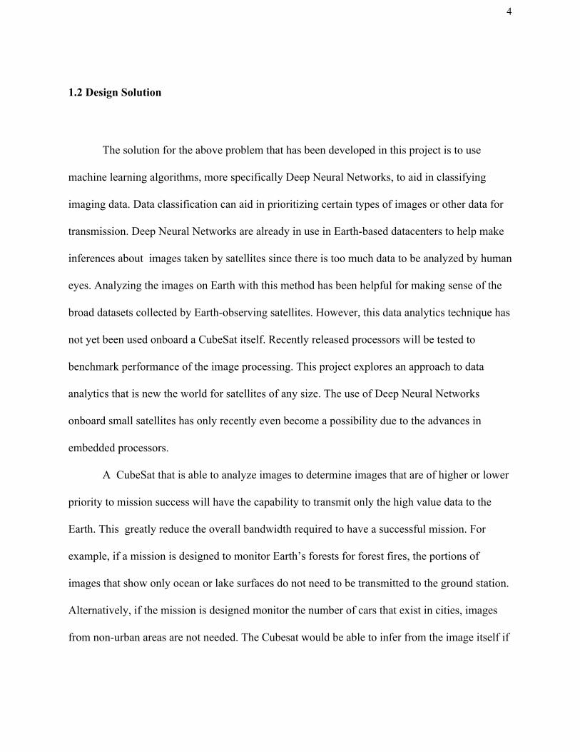
1.2 Design Solution

The solution for the above problem that has been developed in this project is to use

machine learning algorithms, more specifically Deep Neural Networks, to aid in classifying

imaging data. Data classification can aid in prioritizing certain types of images or other data for

transmission. Deep Neural Networks are already in use in Earth-based datacenters to help make

inferences about images taken by satellites since there is too much data to be analyzed by human

eyes. Analyzing the images on Earth with this method has been helpful for making sense of the

broad datasets collected by Earth-observing satellites. However, this data analytics technique has

not yet been used onboard a CubeSat itself. Recently released processors will be tested to

benchmark performance of the image processing. This project explores an approach to data

analytics that is new the world for satellites of any size. The use of Deep Neural Networks

onboard small satellites has only recently even become a possibility due to the advances in

embedded processors.

A CubeSat that is able to analyze images to determine images that are of higher or lower

priority to mission success will have the capability to transmit only the high value data to the

Earth. This greatly reduce the overall bandwidth required to have a successful mission. For

example, if a mission is designed to monitor Earth’s forests for forest fires, the portions of

images that show only ocean or lake surfaces do not need to be transmitted to the ground station.

Alternatively, if the mission is designed monitor the number of cars that exist in cities, images

from non-urban areas are not needed. The Cubesat would be able to infer from the image itself if

5

it is valuable for the mission and discard or de-prioritize images with lower informational value.

Also, sections of images where the scene is obscured, such as cloud cover in a visible light

image, can be deprioritized for transmission.

1.3 Motivations

The use of machine learning techniques are becoming more widespread across many

areas in commerce, robotics, and nearly every field that deals with large amounts data. Small

satellites are constantly borrowing from technologies that are present in commercial and

commodity products. The miniaturization of processors has reached the point where Cubesats

can wield great computational power on their miniscule power and size budgets. Following this

trend of borrowing from other technological areas, this project is an attempt to take data

interencing seen on terrestrial robotics into space. This project was used to expand the author’s

knowledge in the field of Deep Learning as well as trying to find novel approaches for Cubesat

data processing.

1.4 List of Acronyms and Abbreviations

DNN - Deep Neural Network

DIGITS - NVIDIA Deep Learning GPU Training System

GPU - Graphics Processing Unit

CPU - Central Processing Unit

RAM - Random Access Memory

6

SDK - Software Development Kit

API - Application Programming Interface

NCSDK - Neural Compute Software Developer Kit

COTS - Commercial off-the-shelf

TX2 - Nvidia Jetson TX2 System on a Module

NCS - Neural Compute Stick

RGB - Red Green Blue

CUDA - Compute Unified Device Architecture

cm - centimeter

kg - kilogram

GB - Gigabyte

MB - Megabyte

FLOPS - Floating Point Operations Per Second

TRL - Technology Readiness Level

7

2. Relevant Technical Issues

2.1 CubeSats

CubeSats are a type of small satellite that are typically developed to reduce the cost and

development time of a space mission. The CubeSat design standard was developed in 1999 by

California Polytechnic State University. CubeSats are made of multiples of 10x10x10 centimeter

cubes with each cubic unit having a mass of no more that 1.33 kilograms [1]. The motivation to

produce small, standard-sized satellites was to combat the typical design cycle of a satellite

mission that results in several years to decade long development periods an hundreds of millions

of dollar budget requirements. While the first CubeSats often lacked enough capability to be

considered more than a toy or educational experience for the developers, as technology becomes

smaller, more capable, and more accessible, CubeSats can be launched with more and more

capabilities.

8

Figure 2.1: 1U CubeSat

To decrease development time and budget, CubeSats are typically developed with

Commercial-Off-The-Shelf (COTS) components. Larger, hundred-million-dollar satellites are

often unable to utilize parts such as these because COTS components that have been developed

for terrestrial application insert a significant amount of risk into a satellite mission. The

comparatively low cost of a CubeSat mission allows missions to be designed with higher risk

levels. With some considerations, cutting edge COTS components that were designed to be use

in terrestrial applications can be implemented in CubeSats in ways that traditional satellite

designs could never not consider.

9

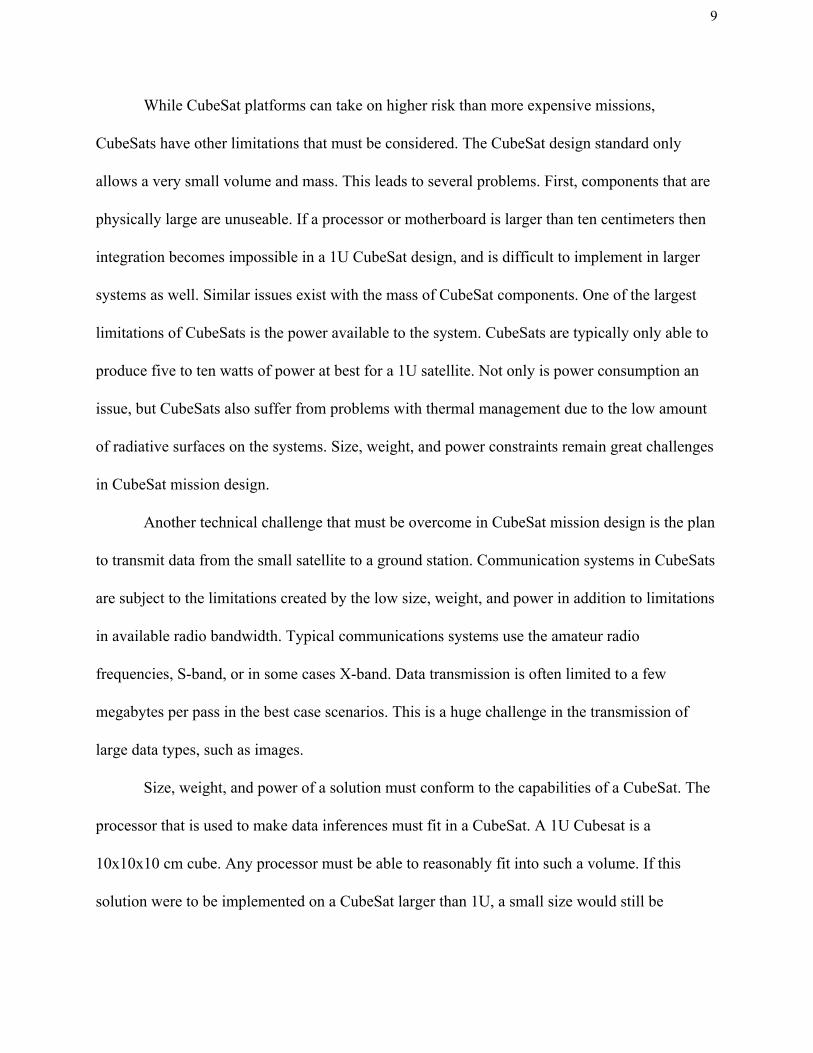
While CubeSat platforms can take on higher risk than more expensive missions,

CubeSats have other limitations that must be considered. The CubeSat design standard only

allows a very small volume and mass. This leads to several problems. First, components that are

physically large are unuseable. If a processor or motherboard is larger than ten centimeters then

integration becomes impossible in a 1U CubeSat design, and is difficult to implement in larger

systems as well. Similar issues exist with the mass of CubeSat components. One of the largest

limitations of CubeSats is the power available to the system. CubeSats are typically only able to

produce five to ten watts of power at best for a 1U satellite. Not only is power consumption an

issue, but CubeSats also suffer from problems with thermal management due to the low amount

of radiative surfaces on the systems. Size, weight, and power constraints remain great challenges

in CubeSat mission design.

Another technical challenge that must be overcome in CubeSat mission design is the plan

to transmit data from the small satellite to a ground station. Communication systems in CubeSats

are subject to the limitations created by the low size, weight, and power in addition to limitations

in available radio bandwidth. Typical communications systems use the amateur radio

frequencies, S-band, or in some cases X-band. Data transmission is often limited to a few

megabytes per pass in the best case scenarios. This is a huge challenge in the transmission of

large data types, such as images.

Size, weight, and power of a solution must conform to the capabilities of a CubeSat. The

processor that is used to make data inferences must fit in a CubeSat. A 1U Cubesat is a

10x10x10 cm cube. Any processor must be able to reasonably fit into such a volume. If this

solution were to be implemented on a CubeSat larger than 1U, a small size would still be

10

preferable to allow room for other payloads on the satellite. The power budget of a CubeSat

limits the available power that can be provided to a processor to just a few watts per CubeSat

Unit. The maximum power of processors examined in this project will need to remain under

about ten watts, which is about the maximum a processor could possibly be allowed on a 3U

CubeSat. Higher power consumptions could possibly be implemented, but this ten watt figure

provides a general goal.

The solution provided for this data analytics must also be able to survive the space

environment. Most COTS hardware is designed with the terrestrial environment in mind, making

them susceptible to malfunctions due to thermal problems, the radiation environment in space, or

other complications from the space environment. Finding hardware that operates in space is a

considerable problem and CubeSat designers often resort to only implementing hardware that

already has flight heritage. This strategy of only flying components that have flown before will

not be useful for this study since this data analysis technique has not been implemented on any

satellite mission, CubeSat or larger, known to the author.

The computational power required for processing images with neural networks greatly

surpasses what is typical on a CubeSat. Hardware must be chosen that is capable of completing

the calculations in a small enough time to be worthwhile to the satellite mission. An inference to

a single image requires millions of floating point operations. The data inference system designed

must be able to analyze an image in a few seconds. If inference takes too long, the CubeSat may

not be able to keep up with image capture and/or data transfer to Earth.

11

2.2 Deep Learning

Artificial Neural Networks are a machine learning technique that are inspired by the

connected systems of biological neural networks in the human brain. They are able to ‘learn’ by

considering data examples that are fed into the algorithm. An example of a use for this would be

image classification. An Artificial Neural Network might be trained to identify that an image is

either a cat or a dog by training the algorithm on thousands of images of that have been labelled

as cats or dogs. The process of using a DNN to classify and image requires first that the DNN in

trained on a dataset. After the DNN is trained, the algorithm can then be used in runtime to make

data inferences. Neural Network mathematics, the process of training, and the requirements for

runtime inferencing will be explained further in the following paragraphs.

Artificial Neural Networks are made up of a collection of nodes, referred to as artificial

neurons. These nodes are connected to one another and can transmit signals to one another.

Layers of these artificial neurons have ‘synapses’ that are connected between artificial neurons to

form a Neural Network. Each artificial neuron receives a signal, processes the signal, and then

sends the processed signal to the artificial neurons connected to it. Typically these artificial

neurons are arranged in layers, and the neurons feed numerical values to one another. When a

neural network has multiple layers between the input and the output it is said to be “deep” i.e. the

phrase Deep Learning . Data is given to the DNN through the input layer. Each neuron in the

input layer processes the input, then passes the processed signal to the next layer, an so on until

final signals come out of the output layer. Typically the processing that happens within each

artificial neuron is some variation of a non-linear scaling of the sum of its inputs. This is called

12

an activation function. The output of this nonlinear function is sent out through each synapse.

Each synapse multiplies the the value that is being passed through it by some weight. The

processing of designing a neural network involves choosing how many layers exist in the

network, how each layer and artificial neuron is interconnected, and which activation functions

to use in each artificial neuron, and several other hyperparameters . The process of training a

neural network involves adjusting the weights on each synapse. The following is an image that

represents a simple neural network.

Figure 2.2: Example of Simple Neural Network Design

13

In Figure 2.2, a simple neural network is depicted with an Input Layer containing three

inputs, a single hidden layer with four neurons, and an Output Layer with two output neurons.

Each circle represents a neuron and each arrow represents a synapse. A neural network such as

this could be trained to take in three data points and provide two outputs. An example of such a

situation could be trying to determine if a student was going to pass or fail an exam. In such a

scenario, the input data could be the number of minutes the student studied, the number of hours

the student slept the night before the exam, and the student’s current grade in the class. The two

output neurons would infer whether the student would pass the test or fail the test. If the input

data indicated the student was going to pass, the first output neuron would have a value close to

1 and the second output neuron would be close to 0. If the input data indicated the student was

going to fail, the values in the output neuron would be vice versa. This is an example of a

classification problem. An input is fed into a neural network and an output is given to be one of

certain number of classes.

The mathematics of how a neural network would make an inference starts at the input

layer. With three inputs (x1, x2, x3) and a synapse between every input node and every neuron in

the hidden layer with weights W1-1, W1-2, W1-3, W1-4, W2-1, W2-2, …., W3-4, the numerical

calculation to take the input values to the input of the hidden layer would be the following:

14

Figure 2.3: Matrix Multiplications between Neural Network layers where x is output from

previous layer, W is the weight of each synapse, and i in the input of the next layer.

The outputs of the weighted inputs would then be used as the input of the activation

function in each neuron in the hidden layer. The activation function is what introduces

non-linearity into a neural network. Without this activation function, a neural network would

become a linear regression model. By introducing an activation function at each neuron, a neural

network is able to make inferences on much more complicated dataset. Originally the sigmoid

function was a commonly used activation function because they are easy to manipulate

mathematically. Now rectified linear unit (ReLu) or similar functions are most commonly used

as activation functions due to performance increases. These two functions and their plots are

shown in the following figure.

15

Figure 2.4: Sigmoid Function

Figure 2.5: ReLu Function

After the activation function is performed on the neuron inputs, the calculated value is

then passed through the synapses into the next layer of the network. This process is repeated for

each layer in the network. In the example given above, an inference on the input data may take

only about a few hundred floating point operations in a computer. This is certainly achievable for

most processors to compute in a reasonable time. However, such a simple data analysis is not the

16

typical use case for a DNN. A typical image inference uses each pixel as an input in the input

layer. GoogleNet, as an example, uses a 224x224 pixel RGB image as the input [2]. That is over

150,528 neurons in the input layer alone. Additionally, typical DNNs certainly have more than

one hidden layer. AlexNet, a DNN from 2012 that started the ‘Big Bang’ of Deep Learning, has

seven layers [3]. GoogleNet has twenty-two layers. Other DNN architectures exist with even

more than that. To make a data inference on an image using Deep Learning, billions to trillions

of operations must be performed. This number of operations simply cannot be computed fast to

enough to be useful on most processors that could fit the size, weight, and power requirements

for a CubeSat.

The explanations in previous paragraphs showed how a data inference is made at run time

with a DNN. However, before a DNN is useful, it must be trained on how to make those

inferences. The process of training requires a vast training dataset. For image classification,

which is the technique used in this project, each of the training images must also be labelled as to

which class the image belongs to. This is because image classification is a form of supervised

learning, where a computer learns how to inference data based on thousands to millions of

pre-labelled examples given to it by a human. Training a DNN involves adjusting the weights on

each synapse in the network. This adjustment is done by entering each piece of data in the

training dataset into the DNN, then checking the output against the label that the training data

belongs to. Starting from the synapses closest to the output layer, the weights that cause the most

error in the output of the DNN is adjusted using Stochastic Gradient Descent or other algorithm

designed for this purpose. This process of sending training data through the DNN, then adjusting

the errors starting from the weights closest to the output of the DNN is called Backpropagation .

17

The training process requires significantly more computational resources than using a

DNN in runtime. The mathematics for Stochastic Gradient Descent demand a great deal of

computations and this backpropagation is done for every single data point in the training data

multiple times while training. If a training dataset has one million images in it and the training

process uses thirty epochs of backpropagation, the DNN will be adjusted thirty million times in

training with each adjustment requiring millions to billions of operations each.

Figure 2.6: 2-Dimensional Representation of Stochastic Gradient Descent, where J(w) is the

output of the cost function that measures the error in the DNN

While the above example was an instance where Deep Learning could be used to classify

images, several other machine learning problems can be solved with DNNs. As stated

18

previously, classification is when data is processed and labelled to belong to one of many

predefined classes of data, such as classifying that an image is an image of a cat. DNNs can also

perform detection. This would be where a neural network could determine if a cat was in an

image and where the cat was located within the image. Image segmentation can also be

performed by DNNs. Image segmentation is when an image is broken down pixel by pixel to

determine what objects exist in each area of the image. Segmentation can be used to do image

processing important for self-driving cars such as determining which pixels in an image are the

road, which pixels are the sidewalk, and which pixels are cars. DNNs are not limited to image

data. Very interesting work in Deep Learning is being done with time-series data. Companies are

using DNNs to predict stock prices, make Radio Frequency noise filters, perform image

restoration, perform speech analysis, cut highlight clips from sports games, play video games,

and many more uses [10] [11] [12] [13].

Figure 2.7: Image processing examples possible with DNNs

Credit: Nvidia

19

It wasn’t until the last decade that computers with enough computational power to

perform training or runtime calculations for DNNs even existed. Because of this, Deep Learning

is still a very new field. While the mathematics describing neural networks were invented in the

1940’s, it was not practical until computers could calculate the output of a neural network in just

a few seconds. Because of the sheer number of calculations required to make a data inference

using Deep Learning, it is still most commonly performed at data centers with powerful compute

clusters or on servers and computers with large, power hungry Graphical Processing Units

(GPU). The computations needed for DNNs lend themselves well to being performed on GPUs

because the matrix calculations needed can be parallelized. GPUs excel in parallel computation.

As computers have gotten powerful and more power efficient, Deep Learning has crept

into more and more uses. It is likely that the reader has used Deep Learning today, even if they

do not realize it. Amazon uses Deep Learning to process human speech for its Alexa enabled

devices. Netflix uses Deep Learning to recommend what movies to watch. Facebook uses DNNs

to determine which ads to serve users. Google, Tesla, and several other autonomous vehicle

companies are using Deep Learning in the development of self-driving technology. Billions of

dollars have been poured into Deep Learning research and more and more uses are being

discovered for them everyday. One of the areas of research is how to do more data inferencing

on the edge , rather than in a data center far away from the device collecting the data. DNNs are

being designed that require less computation. More importantly for this project, hardware is

being designed specifically for Deep Learning at the edge. This hardware is being designed for

low size, weight, and power uses such as robotics, mobile devices, or other small electronics.

20

This could be of great use for a CubeSat developer. The movement of DNN inference to CubeSat

platforms could be the first instance of DNNs in space, at the far edge.

Even though some inferencing can now be done on the edge, the processing of training a

DNN still lives in a workstation or data center not suitable for low size, weight, and power

systems. The performance of a DNN for its intended task largely depends on the size and quality

of the training data that is used to train it. This can be a deal breaker for some potential uses for

DNNs. In some cases, training data may not be available in the quantities required because it has

either never been gathered or is difficult to gather. The data that makes up the training dataset

should closely represent the data that the DNN will receive for inferencing at runtime. Also, for

supervised learning such as image classification and detection, the dataset must be labelled so

that the training process can correct itself from the labels. This process of labelling images can

be difficult and tedious. Typical image datasets for image classification contain at least tens of

thousands of images, with all images being labelled as the class that the DNN should output. A

typical rule of thumb for training dataset size is that there should be no fewer than one thousand

images for each class that is being classified.

21

3. Design Tradeoffs

3.1 Considerations

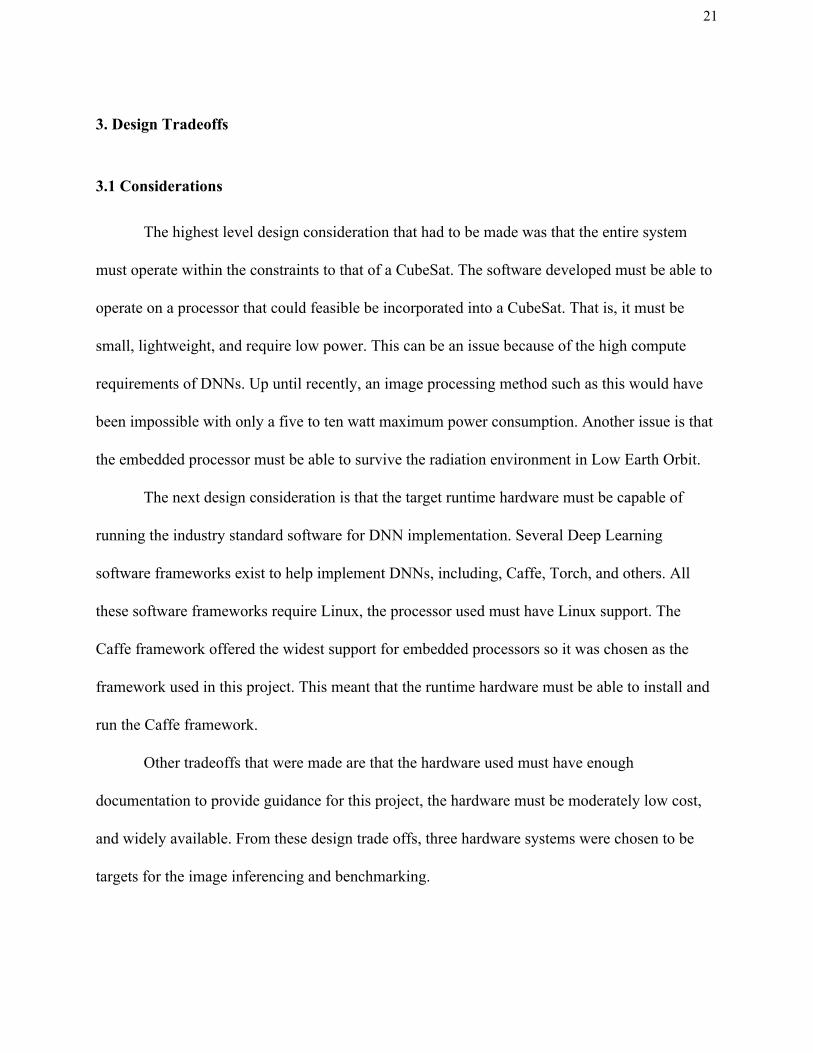
The highest level design consideration that had to be made was that the entire system

must operate within the constraints to that of a CubeSat. The software developed must be able to

operate on a processor that could feasible be incorporated into a CubeSat. That is, it must be

small, lightweight, and require low power. This can be an issue because of the high compute

requirements of DNNs. Up until recently, an image processing method such as this would have

been impossible with only a five to ten watt maximum power consumption. Another issue is that

the embedded processor must be able to survive the radiation environment in Low Earth Orbit.

The next design consideration is that the target runtime hardware must be capable of

running the industry standard software for DNN implementation. Several Deep Learning

software frameworks exist to help implement DNNs, including, Caffe, Torch, and others. All

these software frameworks require Linux, the processor used must have Linux support. The

Caffe framework offered the widest support for embedded processors so it was chosen as the

framework used in this project. This meant that the runtime hardware must be able to install and

run the Caffe framework.

Other tradeoffs that were made are that the hardware used must have enough

documentation to provide guidance for this project, the hardware must be moderately low cost,

and widely available. From these design trade offs, three hardware systems were chosen to be

targets for the image inferencing and benchmarking.

22

3.2 Nvidia Jetson TX2

The first system chosen was the Nvidia Jetson TX2. The TX2 is a System on a Module

developed by Nvidia specifically for artificial intelligence on at the edge. It consists of two

multi-core ARM processors and has a 256 CUDA core GPU onboard. This hardware was chosen

because it was designed specifically for applications such as these. This processor has been

implemented in a plethora of industry robotics, video analytics, image processing, and other

compute intensive tasks that are conscience of power consumption and size. The TX2 comes

with incredible documentation and software tools to allow development on the platform to be

very approachable. This processor is has the highest power consumption of the hardware types

tested here, but provides by far the highest performance. The power consumption can be adjusted

between ~5 watts and ~12.5 watts. One major drawback of this system is that no similar

hardware has ever been flown in space and it is difficult to know how the hardware would

behave in the radiation environment of Low Earth Orbit. No GPU has ever been flown in space,

and the specific ARM chips used in the TX2 also have limited to no flight heritage. Significant

risk would be incurred if this processor was used on a CubeSat. Specifications for the TX2, and

Nvidia’s older version, the Jetson TX1 can be found in the following figure:

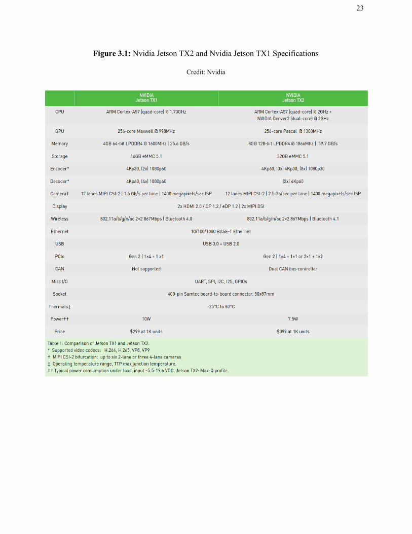
23

Figure 3.1: Nvidia Jetson TX2 and Nvidia Jetson TX1 Specifications

Credit: Nvidia

24

Figure 3.2: Nvidia Jetson TX2 Development Kit

Figure 3.3: Nvidia Jetson TX2 Module

Credit: Nvidia

25

3.3 Raspberry Pi 3 B

The Raspberry Pi is one of the most common consumer/commodity microprocessors. Its

availability, low price, and extensive resources and tutorials make it a common first step into the

world of embedded processors. Its ubiquity in the market makes it familiar with many engineers

so benchmarking on this platform is a good starting point to understand the performance of DNN

inferencing. This is lowest capability hardware tested. While the hardware has the lowest

computational power, it does have limited flight heritage such as the Astro-Pi project on the

International Space Station [14]. Specifications for the Raspberry Pi 3 B can be found in the

following figure.

Figure 3.4: Raspberry Pi 3 B Specifications

Credit: Hackaday.com

26

Figure 3.5: Raspberry Pi 3 B

3.4 Movidius Neural Compute Stick

The Neural Compute Stick (NCS) made by Movidius is an embedded specialty processor

that is made to perform artificial intelligence algorithms at the edge. It is a USB device that

contains a low power visual processing chip that it meant to augment the processing power of

small embedded devices, such as a Raspberry Pi. The NCS can be used with any x86_64

computer running Ubuntu 16.06 or a Raspberry Pi with Debian Stretch installed. This makes it a

very useful device for rapid prototyping, validation, and deployment of DNNs. For this project,

the NCS us used in conjunction with a Raspberry Pi 3 B. This system is greatly superior than the

Raspberry Pi alone, but is not as high of performance as the Nvidia Jetson TX2. This product and

chipset that it uses has been on the market for less than a year, so no flight heritage or

information about radiation tolerance is available. Also, the temperature range for the device is

well out of what is required for the space environment. It is possible that the visual processing

chipset used could be updated to have better temperature range capabilities, or future similar

27

products could be more suitable. Once again, the reliability of the device in the space

environment is traded for the performance the hardware provides. Specifications for the device

are in the following figure.

Figure 3.6: Movidius Neural Compute Specifications

28

Figure 3.7: Movidius Neural Compute Specifications

Figure 3.8: Movidius Neural Compute Stick Installed in Raspberry Pi 3 B

29

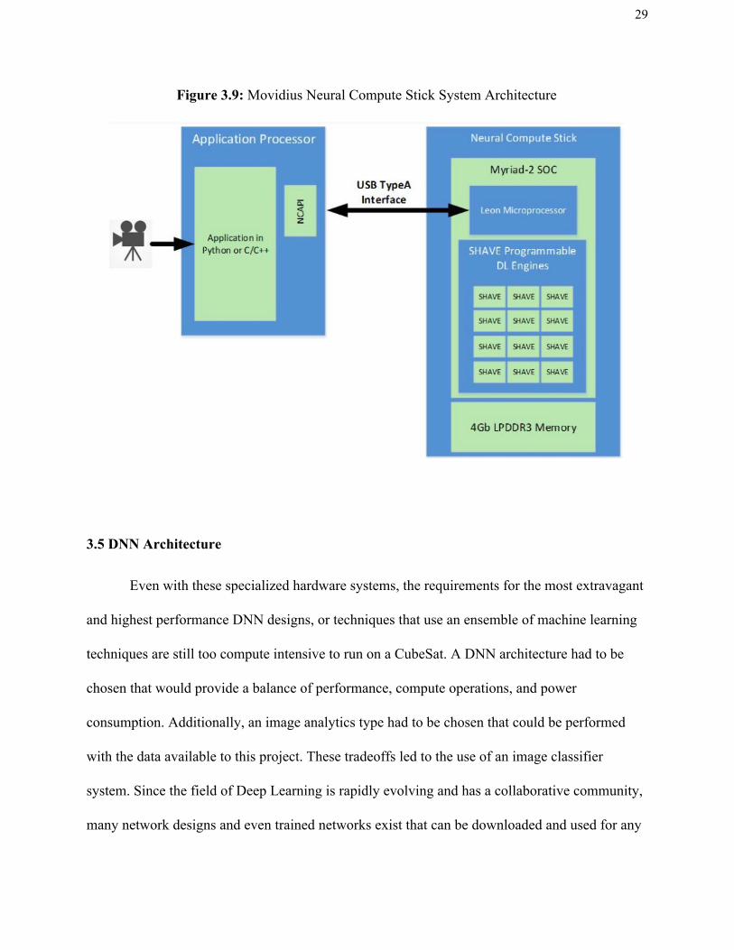
Figure 3.9: Movidius Neural Compute Stick System Architecture

3.5 DNN Architecture

Even with these specialized hardware systems, the requirements for the most extravagant

and highest performance DNN designs, or techniques that use an ensemble of machine learning

techniques are still too compute intensive to run on a CubeSat. A DNN architecture had to be

chosen that would provide a balance of performance, compute operations, and power

consumption. Additionally, an image analytics type had to be chosen that could be performed

with the data available to this project. These tradeoffs led to the use of an image classifier

system. Since the field of Deep Learning is rapidly evolving and has a collaborative community,

many network designs and even trained networks exist that can be downloaded and used for any

30

use. These trained models exits in “Model Zoos” from several different sources. Since no

pre-trained model existed to perform the exact image classification done within this project, a

DNN was trained specifically for the use in this project. Also, to make the benchmarks

performed in this project as relevant to future work as possible, a well known DNN architecture

should be chosen rather than an obscure or custom design. A common, high performance image

classifier network design called GoogleNet [2] was used as the DNN architecture to balance all

the trade offs considered.

31

4. Design Implementation

The solution designed was an image analysis software system that could be run on

hardware that could be implemented within the size, weight, and power constraints of a CubeSat

system. The image analysis takes a large, high resolution image of Earth’s surface and classifies

small regions within the image as being either covered with clouds, covered in water, a city

environment, or non of the other classes. The image analysis software was then benchmarked on

the intended hardware to provide a baseline performance measurement for future work with

DNNs on CubeSats. The implementation of this design is explained in the following sections.

4.1 Nvidia DIGITS Workstation

Nvidia DIGITS is a tool provided by Nvidia for creating Deep Learning dataset and for

training neural networks. DIGITS simplifies common deep learning tasks such as managing data,

designing and training neural networks on multi-GPU systems, monitoring performance in real

time with visualizations while training, and selecting the best performing model from the results

browser for deployment. DIGITS was installed on an Ubuntu workstation at the Morehead office

of Rajant Corporation. This workstation was built with an Intel i7 processor, 32GB of RAM, and

two Titan xP GPUs. The DIGITS tool was made accessible with a web browser within the local

network of the Morehead Rajant Corporation office.

32

4.2 Creating a Dataset

In order to implement a DNN Classifier, the DNN must be trained on a large dataset.

Data collection, curation, and implementation was a significant effort for this project. The

following paragraphs will explain the process of collecting and curating the dataset.

The first task for choosing a dataset was deciding on a source for the images. First and

foremost, the images must represent the type of data that one could expect to obtain on an Earth

observing satellite. In this case, this means the dataset must be built from images of Earth’s

surface taken from satellites. Secondly, the dataset must have clear distinctions between the

classes of data that this project seeks to classify. The dataset must include examples of all the

different classes that are to be classified. It must show areas covered in water, areas with cloud

obstruction, areas of cities, and other areas. A source for images that could result in a successful

project must give access to tens of thousands of smaller (512x512 pixels) or give access to

hundreds of larger images. The goal for this project was to have 20,000 images in the training

dataset so a vast amount of source data is required. Results for this project will be optimal if the

image quality of training data is consistent, and conditions of how the images were obtained and

processed were consistent with both the rest of the training data and the data that the final trained

algorithm will be inferencing during run-time. Lastly, for quality of life for the data curator, a

dataset that is straightforward to obtain, curate, and hand classify is optimal.

The pool of possible candidates for source data was the following: web crawling Google

image results, finding a pre-curated dataset, or finding a satellite mission that provides public

access to raw or minimally processed images. Web crawling was not chosen because image

33

quality and consistency could not be guaranteed without considerable effort. This could have

been successful, but was far from optimal. Finding a pre-curated dataset would have been the

optimal path if such a dataset existed. Several services exist that allow users to share and obtain

curated data. One such place for this is kaggle.com, which is a website dedicated to machine

learning competitions, datasets, and learning resources. After searching Kaggle for an

appropriate dataset, this idea was also abandoned. No dataset existed that was perfect for this

project. The final option, and the method that was utilized in the end was to access data that has

been released from previous satellite missions and curate this data.

The dataset was created with data obtained from Planet Labs, using their Planet Explorer

web application. With a free account, a user can obtain free data from seven different satellite

image sources. This free account is only allowed access to imaging data that is a few weeks old

or older and images taken of the state of California. These limitations were of no consequence

for the creation of this dataset since it was still possible to obtain thousands of consistent, high

quality images featuring all four classes of images required. Additionally, the Planet Explorer

web application had many features that made obtaining the raw images very user friendly.

The Planet Labs data repository offers imagery collected from several sources, including

PlanetScope, RapidEye, Skysat, Sentinel 2, and Landsat 8. Source images from PlanetScope

were chosen for the training set because it contains the highest resolution imagery and the largest

number of accessible images. Within the PlanetScope imagery, four-band (red, green, blue, and

near infrared) and three-band (red, green, and blue) images are available. The dataset created

used the there-band images because the input layer of typical image classifier networks only

accepts three color bands. The color depth of the downloaded images was 8-bit. Higher bit-depth

34

(16 bit) imagery was available but not required for this dataset. If the performance of the DNN

classifier was not high enough to be useable, the higher color depth images could have been

used.

Once the raw images were obtained from Planet Labs, more processing was required to

produce a usable training dataset. A typical image from Planet Labs was about 8000-9000 pixels

wide. The raw images are also oriented to north and south. Since the satellite passes are done at a

non-zero inclination, the raw images show a diagonal swath of land. In order to make the image

rectangular, the blank areas of the raw image are filled with black pixels.

Figure 4.1: Example of Raw Image Downloaded from Planet Explorer

35

The goal of this project is be able to classify small areas of Earth’s surface so the training

data needs to show smaller regions that what is depicted in these large images. Additionally, the

input layer of a typical image classify DNN accepts a 224 x 224 pixel image. If one of these

large, 9000 pixel wide images were used as training data, it would be squashed to 224 x 224 in

the preprocessing step of the final algorithm so much of the high detail would be lost. These

large, raw images were tiled into smaller 512 x 512 pixel images to create the training set. This

tiling process also has the benefit of creating dozens of training images from a single raw image,

and allowed the final algorithm to be able to classify smaller areas of land. This helped with

obtaining enough images to produce a training dataset. Before tiling, the images were rotated so

that the swath of land could be cropped into a rectangle and the black filler pixels could be

removed. This process resulted in approximately 80 512x512 pixel image tiles for each raw

image downloaded from the 3-band Planetscope Scene database. The scripts used to rotate and

crop the source images, then tile the images can be found in section 8.1.

Figure 4.2: Rotated and Cropped Source Image

36

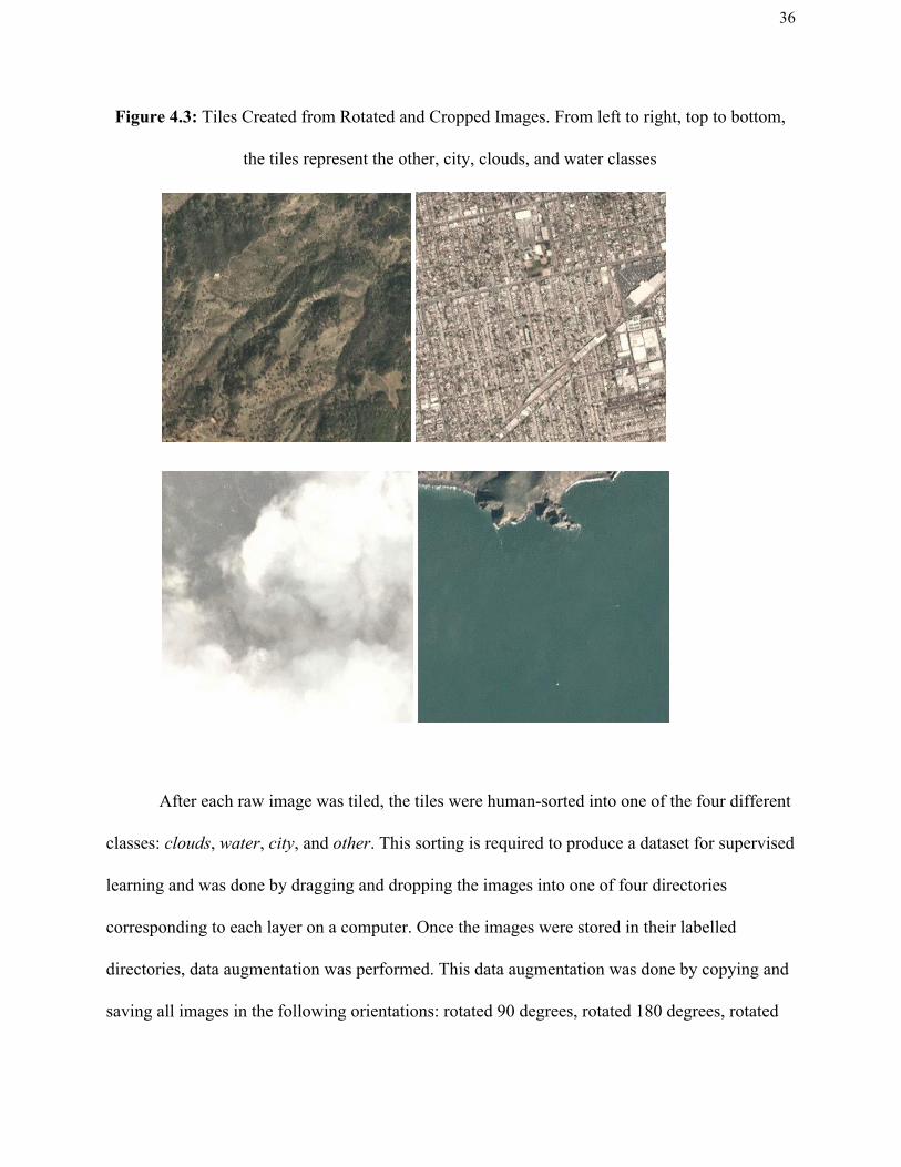
Figure 4.3: Tiles Created from Rotated and Cropped Images. From left to right, top to bottom,

the tiles represent the other, city, clouds, and water classes

After each raw image was tiled, the tiles were human-sorted into one of the four different

classes: clouds , water , city , and other . This sorting is required to produce a dataset for supervised

learning and was done by dragging and dropping the images into one of four directories

corresponding to each layer on a computer. Once the images were stored in their labelled

directories, data augmentation was performed. This data augmentation was done by copying and

saving all images in the following orientations: rotated 90 degrees, rotated 180 degrees, rotated

37

270 degrees, flipped horizontally, and flipped vertically. This results in 6 total training images

from each tile, and about 500 training images for each raw image from Planet Labs. Data

augmentation was performed after sorting the tiles because it reduces the amount of data that

required manual sorting. While the augmented images are different enough to provide valuable

training images, the augmentation does not change which class they belong to so all 6 iterations

of a tile can remain in the same labelled directory. This data augmentation was performed by the

script “augmenter.py” shown in section 8.1.

After the raw data was split into tiles and augmented, the tiled and augmented dataset still

requires some manipulation to optimize the dataset for training the Googlenet image classifier.

The Nvidia DIGITS tool was used to finish the dataset processing. The labelled images were

uploaded to the DIGITS server. For the final processing of the dataset, the images were resized

with a squash transformation to 256 x 256 pixel images, converted to PNG image format, and

saved in an Lightning Memory-Mapped Database, which is a typical database used for dataset

storage in Deep Learning. The images were separated into training images, validation images,

and testing images. This finalized the training dataset creation.

4.4 Training the Deep Neural Network

One of the strengths of DNNs is that the layers of the network can be designed to do a

great number of data inference tasks. Many neural network designs are freely available and

openly documented due to the quickly evolving nature of the field of deep learning. Papers are

published every day with new advances in the field. Rather than designing a neural network

specifically for the use of this project, a suitable network design was chosen. This was due to

38

many reasons. First, the scope of this project was to find, implement, and benchmark a practical

use of deep learning on a cubesat, rather than to delve deep into neural network design. Second,

several neural network designs already exist that provide sufficient performance for the uses of

this project. The systems level approach of choosing a premade neural network architecture was

more suitable for this project.

Googlenet was chosen for the neural network architecture. Googlenet was published in

2014 [2]. It was developed for the ImageNet competition, which was a competition for image

classification algorithms. GoogleNet was the first image classification algorithm that scores as

well as humans on the dataset provided for the ImageNet challenge. Due to its performance, and

the fact that it is one of the most widely cited, published, and implemented DNNs, it makes a

great candidate for a project such as this one. GoogleNet has been implemented on nearly every

type of hardware that is capable of deep learning. Tutorials for how to use GoogleNet are

abundant. Because of this, the accuracy of the trained models can be checked against other

published figures and the benchmarks provided by this study can be understood by others who

plan to implement deep learning. An image depicting each layer of GoogleNet can be found in

section 8.3.

After creating the training dataset and choosing the neural network architecture, the next

step was to train the neural network on the dataset. NVIDIA DIGITS was used for this task and

the training took place on the DIGITS workstation at Rajant Morehead. The network was trained

three times with different training parameter settings. The parameter that was adjusted between

different trained models was the process used to normalize the training image. The first trained

model used Mean Image Subtraction, the second model used no mean subtraction, and the third

39

model used Mean Pixel Subtraction. In Mean Image Subtraction, an ‘average image’ is produced

from all images in the dataset by averaging the red, green, and blue values for each pixel

coordinate. This results in 256x256 pixel averages. The average image consisting of each of

these pixel values is subtracted from each training image before being used for training. In Mean

Pixel Subtraction, a single average value for all pixels in the dataset is calculated. This one value

is subtracted from each pixel in an image before being used for training. The Mean Pixel

Subtraction resulted in the highest accuracy of the training and validation dataset. This mean

pixel subtraction model was the model implemented in the run-time software. Several other

parameters could be modified if the performance of the trained network was not good enough to

be implemented. Fortunately, all other parameters could be left to the default values provided by

DIGITS. Once the network is trained, the Caffe model and all supporting files are downloaded

from the DIGITS server to be used in runtime.

40

Figure 4.4: DIGITS Training interface showing parameters used for DNN training

41

Figure 4.5: DIGITS Training interface showing parameters used for DNN training

4.5 Deep Neural Network at Runtime

The next phase of the project was to implement this trained neural network on hardware

that could be fit into a Cubesat or small satellite. Three different hardware systems were chosen

to give a well rounded view of the performance an engineer could expect to see on such a

system. While none of the systems are specially designed with the space environment in mind,

the results of the testing will give a mission designer some range of benchmarks with which to

practically estimate performance. The systems used in this comparison are the Nvidia Jetson

TX2, Raspberry Pi 3 B, and Raspberry Pi 3 B with a Movidius Neural Compute Stick.

42

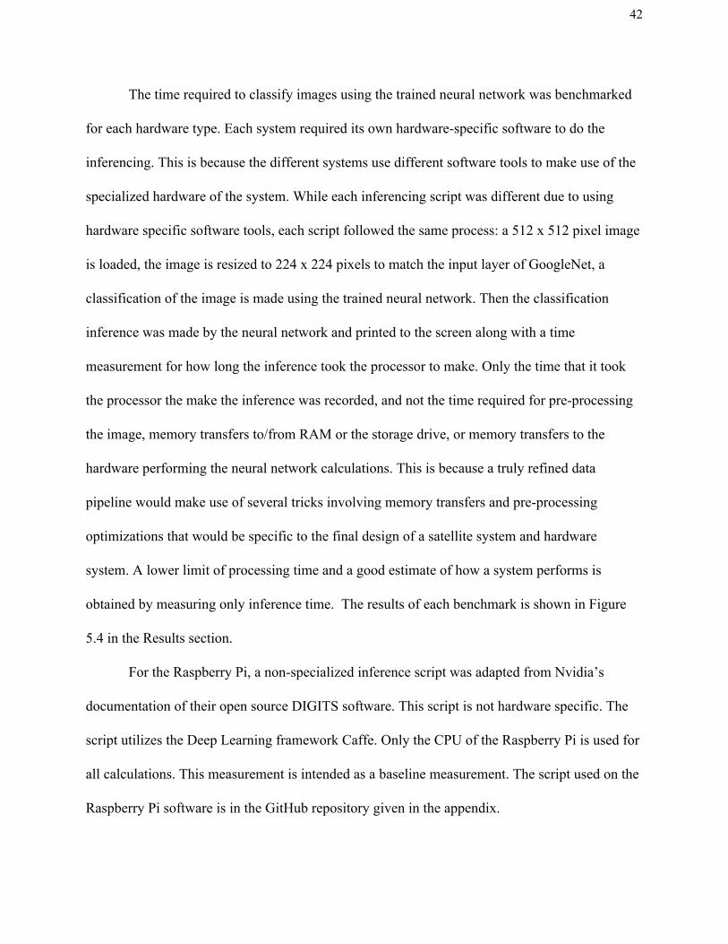
The time required to classify images using the trained neural network was benchmarked

for each hardware type. Each system required its own hardware-specific software to do the

inferencing. This is because the different systems use different software tools to make use of the

specialized hardware of the system. While each inferencing script was different due to using

hardware specific software tools, each script followed the same process: a 512 x 512 pixel image

is loaded, the image is resized to 224 x 224 pixels to match the input layer of GoogleNet, a

classification of the image is made using the trained neural network. Then the classification

inference was made by the neural network and printed to the screen along with a time

measurement for how long the inference took the processor to make. Only the time that it took

the processor the make the inference was recorded, and not the time required for pre-processing

the image, memory transfers to/from RAM or the storage drive, or memory transfers to the

hardware performing the neural network calculations. This is because a truly refined data

pipeline would make use of several tricks involving memory transfers and pre-processing

optimizations that would be specific to the final design of a satellite system and hardware

system. A lower limit of processing time and a good estimate of how a system performs is

obtained by measuring only inference time. The results of each benchmark is shown in Figure

5.4 in the Results section.

For the Raspberry Pi, a non-specialized inference script was adapted from Nvidia’s

documentation of their open source DIGITS software. This script is not hardware specific. The

script utilizes the Deep Learning framework Caffe. Only the CPU of the Raspberry Pi is used for

all calculations. This measurement is intended as a baseline measurement. The script used on the

Raspberry Pi software is in the GitHub repository given in the appendix.

43

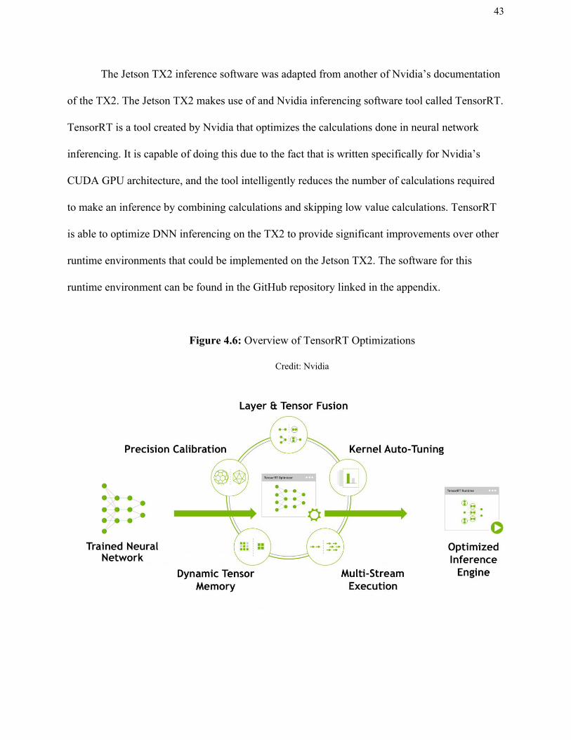
The Jetson TX2 inference software was adapted from another of Nvidia’s documentation

of the TX2. The Jetson TX2 makes use of and Nvidia inferencing software tool called TensorRT.

TensorRT is a tool created by Nvidia that optimizes the calculations done in neural network

inferencing. It is capable of doing this due to the fact that is written specifically for Nvidia’s

CUDA GPU architecture, and the tool intelligently reduces the number of calculations required

to make an inference by combining calculations and skipping low value calculations. TensorRT

is able to optimize DNN inferencing on the TX2 to provide significant improvements over other

runtime environments that could be implemented on the Jetson TX2. The software for this

runtime environment can be found in the GitHub repository linked in the appendix.

Figure 4.6: Overview of TensorRT Optimizations

Credit: Nvidia

44

The Movidius Neural Compute Stick makes use of a special Software Development Kit

and Application Programming Interface to utilize the hardware. Much like TensorRT, the NCS

SDK processes the DNN to optimize its performance on the specialized hardware of the NCS.

The Caffe model that was trained in the training process is compiled by a tool called

mvNCCompile . The output of this tool is a binary of optimized version of the trained DNN. This

binary is called upon during the runtime of the DNN inference and run on the NCS. The SDK

also comes with tools to analyze the performance and timing information of each layer in the

DNN. This tool is of great use in trying to modify DNNs to reduce inference time.

After inference time benchmarking, a full run-time inferencing data pipeline was

developed to demonstrate how a complete image processing system could work on a satellite and

to visualize the results of the classifier. This full inferencing pipeline was developed for use on

the Raspberry Pi with the Movidius Neural Compute Stick. The software was written in Python

and utilizes the NCSDK software provided with the Neural Compute Stick. The full data

inferencing pipeline takes in a large image, tiles the image into 512 x 512 pixel tiles,

preprocesses the tiles for classification, colors the tile red, blue, green, or yellow depending on

which class the tile belongs to, then recombines the tinted tiles back into the original image. The

image coloring is used to visualize the output of the data pipeline for the purposes of this paper.

Four of the resulting images can be found in the following section. The software developed for

the Movidius Neural Compute Stick is section 8.2.

45

5. Results

The final dataset produced in this project consisted of 6903 images in the Training set,

813 images in the validation set, and 404 image in the Test set. Each image was prepared in the

method outlined above. The final dataset size was 656 MB. The original plan for the project was

to produce 20,000 or more training images but the performance of the network trained from this

dataset had sufficient performance. Figures further breaking down the dataset prepared are

shown below.

Figure 5.1: Training Dataset Specifics from DIGITS

46

Figure 5.2: Training Dataset Specifics from DIGITS, showing the amount of images in each

class. From left to right in the bar graph the categories are water , other , clouds , city .

47

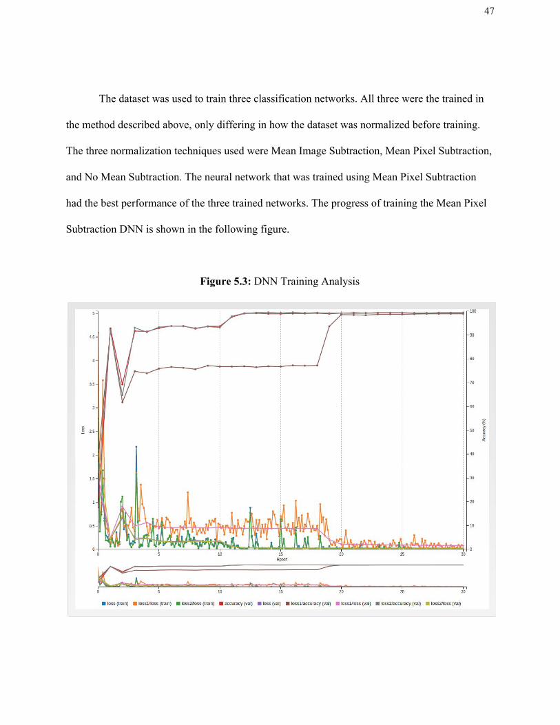
The dataset was used to train three classification networks. All three were the trained in

the method described above, only differing in how the dataset was normalized before training.

The three normalization techniques used were Mean Image Subtraction, Mean Pixel Subtraction,

and No Mean Subtraction. The neural network that was trained using Mean Pixel Subtraction

had the best performance of the three trained networks. The progress of training the Mean Pixel

Subtraction DNN is shown in the following figure.

Figure 5.3: DNN Training Analysis

48

Figure 5.3 shows the progress of the neural network as it is trained. The DNN was trained

for 30 epochs. This means that every image in the training dataset was used for backpropagation

30 times. After each training epoch, the neural network checks the accuracy of the model by

inferencing all the images in the validation dataset. This allows the progress of the training to be

monitored. This plot shows the losses (errors from the output of the DNN compared to the label

of the data that was inferences) of the training and validation datasets and the accuracy that the

model predicts the validation dataset. The takeaways from this plot are that over time the losses

decrease and the accuracy of classifying the validation dataset go up. This plot shows that

overfitting has not occured. Overfitting is when a DNN is “remembers” the training dataset and

their classifications rather than being able to make inferences about new data. In the case of

overfitting, the accuracy of the validation dataset (which are images not used in the training

dataset) would go up to a high accuracy, then the accuracy of the validation set classifications

would decrease as training continues. This trend is not shown in the training analysis. In the end,

the accuracy of classifying the validation dataset is 99.26%.

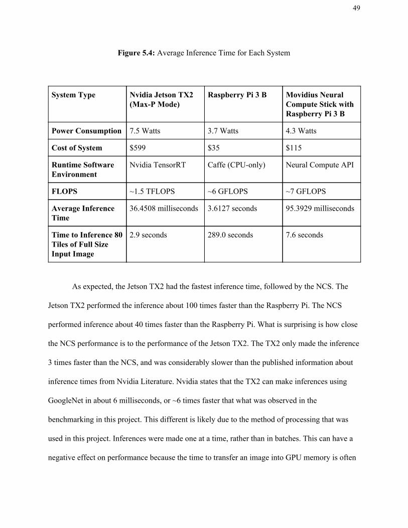
Benchmarking of the trained GoogleNet classifier was performed with the trained DNN.

A summary table is shown in the following figure. The figure shows the average inference time

of each of the systems after 20 or more image inferences.

49

Figure 5.4: Average Inference Time for Each System

System Type Nvidia Jetson TX2 (Max-P Mode)

Raspberry Pi 3 B Movidius Neural Compute Stick with Raspberry Pi 3 B

Power Consumption 7.5 Watts 3.7 Watts 4.3 Watts

Cost of System $599 $35 $115

Runtime Software Environment

Nvidia TensorRT Caffe (CPU-only) Neural Compute API

FLOPS ~1.5 TFLOPS ~6 GFLOPS ~7 GFLOPS

Average Inference Time

36.4508 milliseconds 3.6127 seconds 95.3929 milliseconds

Time to Inference 80 Tiles of Full Size Input Image

2.9 seconds 289.0 seconds 7.6 seconds

As expected, the Jetson TX2 had the fastest inference time, followed by the NCS. The

Jetson TX2 performed the inference about 100 times faster than the Raspberry Pi. The NCS

performed inference about 40 times faster than the Raspberry Pi. What is surprising is how close

the NCS performance is to the performance of the Jetson TX2. The TX2 only made the inference

3 times faster than the NCS, and was considerably slower than the published information about

inference times from Nvidia Literature. Nvidia states that the TX2 can make inferences using

GoogleNet in about 6 milliseconds, or ~6 times faster that what was observed in the

benchmarking in this project. This different is likely due to the method of processing that was

used in this project. Inferences were made one at a time, rather than in batches. This can have a

negative effect on performance because the time to transfer an image into GPU memory is often

50

longer than the time it takes to inference the image. A more efficient inference software that uses

batch processing rather than single image processing would likely reduce the time it takes for the

Jetson TX2 to make an inference. This slowdown in performance from single image processing

does not exist for the CPU processing done in the Raspberry Pi because the image does not need

to transfered to a different memory location. The CPU takes the image directly from RAM rather

than transferring it to GPU memory. The timing information obtained from the NCS took this

memory manipulation into account.

The full image processing pipeline was run on a Raspberry Pi with a Movidius Neural

Compute Stick. The software used to implement this pipeline is shown section 8.2. This image

processing pipeline was completed for several test images. The original image and the results of

the classification are shown in the images below. In the output images, tiles from the water class

are tinted blue, clouds tiles are tinted yellow, city tiles are tinted red, and other tiles are tinted

green. These color tints are used simply as a visualization.

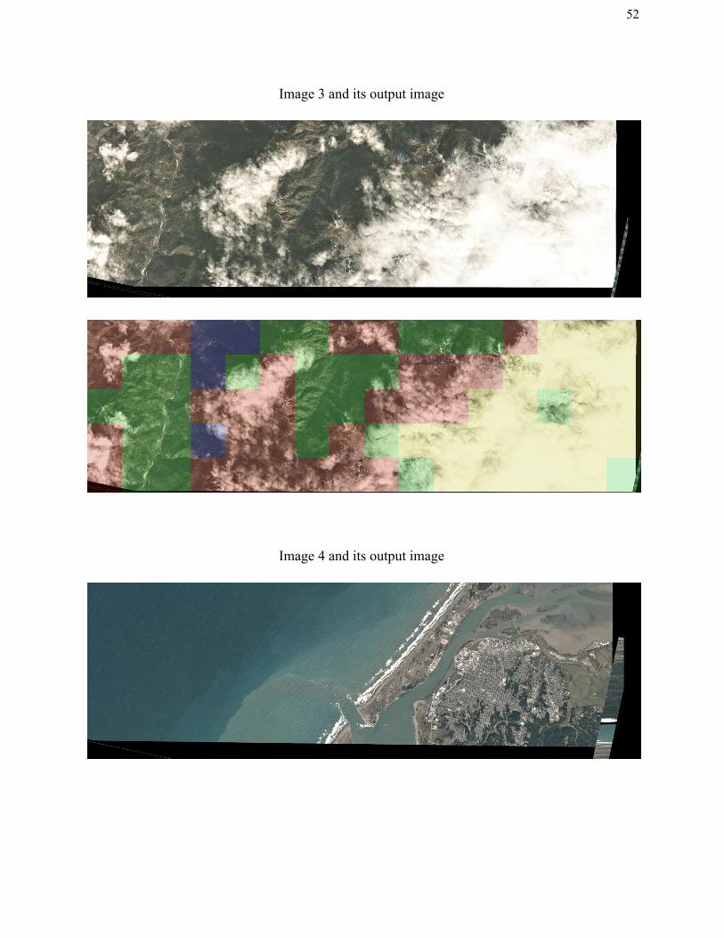
Figure 5.5: Input and Outputs of full data processing pipeline

Image 1 and its output image

51


52



53

Images 1,2 and 4 were processed and the output was as expected. Each area was

classified appropriately. Some limitations of the image analysis strategy were shown. One of

these limitations is that in an area that is half of one class and half of another, how should the

DNN classify the area? This can be seen in the middle of Image 1. One of the tiles is about one

third water and about two thirds other . The data processing pipeline labelled the tile as other , as

it should have, but a CubeSat mission may desire finer tiling than what was used in this project.

Image segmentation may have been an effective strategy rather than classification of several tiles

to solve this issue. Another problem with the image analysis system is apparent in Image 3 and

its output image. Most of the tiles had sparse cloud cover which led to erroneous classifications

of the majority of tiles in the image. The sparse cloud cover caused the confidence of

classification to be comparatively low to the other images. While the classification confidence

for the tiles in Image 1, 2, and 4 were typically 90% and above, the confidences for the tiles in

Image 3 ranged from 50% to 70% for many of the wrongly classified tiles, meaning that the

DNN thought it could possibly be of another class. This problem could be mitigated by retraining

the DNN with more pictures that represent images with sparse cloud cover. Areas with heavy

54

cloud coverage were no problem for the DNN. Additionally, classifications could only be

accepted if confidences were above a certain threshold. If the image was not above this threshold

it could remain unclassified.

55

6. Conclusion

This thesis has found a method of image analysis that has not yet been implemented on

any satellite system by borrowing from cutting edge techniques used in terrestrial robotics and

industry. This method implements Deep Neural Networks, and was implemented on three

different software systems that fit the size, weight, and power requirements of CubeSat Systems.

The performance of each system revealed that it is possible to use DNNs to perform image

analytics on a CubeSat system.

CubeSats could implement this data processing technique by adopting hardware such as

the Nvidia Jetson TX2 or Movidius Neural Compute Stick. However, this would incur great risk

due to the fact that neither system has flown in space. It is not known how they will react in the

radiation environment of Low Earth Orbit. A processor that is of similar capability to a

Raspberry Pi 3 Model B could also be used to run image inferencing with DNNs as long as the

processing was not time sensitive. If the CubeSat took only a few images per ninety minute orbit,

a processing time of five to size minutes would not hinder the mission objective.

Future work based off the results of this thesis could unlock even more potential of using

DNNs in space. Recent developments in Deep Learning have discovered effective DNN designs

that require even less processing power than the GoogleNet DNN used here. Additionally,

hardware that has never been flown before, such as the Jetson TX2 could be tested in satellite

missions to raise its TRL level to acceptable levels to be implemented in future satellite designs.

56

7. References

1. CubeSat Design Specification (13 Revision) [PDF]. The CubeSat

Program, California Polytechnic State University. (2014, February 20). Retrieved from

http://www.cubesat.org/

2. Szegedy, Christian, et al. “Going Deeper with Convolutions.” 2015 IEEE Conference on

Computer Vision and Pattern Recognition (CVPR), 2015,

doi:10.1109/cvpr.2015.7298594.

3. Krizhevsky, Alex, et al. “ImageNet Classification with Deep Convolutional Neural

Networks.” Communications of the ACM, vol. 60, no. 6, 2017, pp. 84–90.,

doi:10.1145/3065386.

4. Goodfellow, Ian, et al. Deep Learning. MIT Press, 2017.

5. “Movidius/Ncsdk.” GitHub, Intel Movidius, 15 Apr. 2018, github.com/movidius/ncsdk.

6. “NVIDIA/DIGITS.” GitHub, Nvidia, 15 Apr. 2018, github.com/NVIDIA/DIGITS.

7. NVIDIA Developer Documentation, 15 Apr. 2018,

docs.nvidia.com/deeplearning/digits/digits-user-guide/index.html.

8. “NVIDIA TensorRT.” NVIDIA Developer, 13 Apr. 2018, developer.nvidia.com/tensorrt.

9. “Planet Platform Documentation.” Planet, 22 Jan. 2018, www.planet.com/docs/.

10. Abdel-Hamid, O.; et al. (2014). "Convolutional Neural Networks for Speech

Recognition". IEEE/ACM Transactions on Audio, Speech, and Language Processing. 22

(10): 1533–1545. doi:10.1109/taslp.2014.2339736.

57

11. Tóth, Laszló (2015). "Phone Recognition with Hierarchical Convolutional Deep Maxout

Networks". EURASIP Journal on Audio, Speech, and Music Processing. 2015.

doi:10.1186/s13636-015-0068-3.

12. G. W. Smith; Frederic Fol Leymarie (10 April 2017). "The Machine as Artist: An

Introduction". Arts. Retrieved 4 October 2017.

13. Schmidt, Uwe; Roth, Stefan. Shrinkage Fields for Effective Image Restoration (PDF).

Computer Vision and Pattern Recognition (CVPR), 2014 IEEE Conference on.

14. “Past Missions.” Astro Pi, 15 Apr. 2018, astro-pi.org/past-missions/.

15. Dustin Franklin. “Dusty-Nv/Jetson-Inference.” GitHub, 12 Feb. 2018,

github.com/dusty-nv/jetson-inference.

58

8. Appendix

All software can be found at the following:

https://github.com/Adam-Braun/MastersThesis

Select Software will be provided in this Appendix

8.1 Python Scripts

8.1.1 cropper.py

#!/usr/bin/env python

from PIL import Image

import glob

target_directory = '/home/adam/Desktop/source_images_rotated'

# filename = '/home/adam/Desktop/source_images/source_14.tif'

for filename in glob.glob(target_directory + '/*.jpg'):

split_name = filename.split('/')

name = split_name[5].split('.')

name = name[0]

print name

img = Image.open(filename)

cropped_image = img.crop((200, 900, 8700, 3600))

# rotated_image.show()

cropped_image.save(name + '_cropped.jpg')

8.1.2 rotator.py #!/usr/bin/env python


import glob

target_directory = '/home/adam/Desktop/source_images'

# filename = '/home/adam/Desktop/source_images/source_14.tif'

for filename in glob.glob(target_directory + '/*.tif'):

59



name = name[0]

print name


rotated_image = img.rotate(348)

# rotated_image.show()

rotated_image.save(name + '_rotated.jpg')

8.1.3 image-tiler.py #!/usr/bin/env python

import cv2

img_file_prefix =

"/home/adam/Desktop/source_images_rotated_cropped/source_"

export_prefix =

"/home/adam/Desktop/source_images_rotated_cropped/tiles/"

index = 1

final_index = 35

while index <= final_index:

img_file = img_file_prefix + str(index) + '_rotated_cropped.jpg'

print 'next source image +++++++++++++++++++++++'

print img_file

img = cv2.imread(img_file)

height, width, channels = img.shape

num_cols = height // 512

num_rows = width // 512

print 'tiling....................................'

for x in range(0, num_rows):

for n in range(0, num_cols):

name = img_file_prefix + str(index) + '_' + str(n) + '_' +

str(x) + '.jpg'

col_pixel_start = (512 * n) + 1

row_pixel_start = (512 * x) + 1

tile = img[col_pixel_start:(col_pixel_start + 512),

row_pixel_start:(row_pixel_start + 512)]

print name

60

split_name = name.split('/')

output_name = split_name[5]

cv2.imwrite(export_prefix + output_name, tile)

index = index + 1

8.1.4 augmenter.py #!/usr/bin/env python


import glob

target_directory = '/home/adam/thesis/images/tiles_batch1/water'

for filename in glob.glob(target_directory + '/*.jpg'):



name = name[0]

print name



rotated_image.save(name + '_90.jpg')





flipped_image = img.transpose(Image.FLIP_LEFT_RIGHT)

flipped_image.save(name + '_flippedLR.jpg')

flipped_image = img.transpose(Image.FLIP_TOP_BOTTOM)

flipped_image.save(name + '_flippedTB.jpg')

8.2 Full Data Pipeline full_pipeline_classifier.py

61

#!/usr/bin/python3

import numpy

import time

import cv2

import mvnc.mvncapi as mvnc

graph_file = 'graph2' # file name of compiled neural network

source_image = 'source_17_rotated_cropped.jpg' # name of image file

to be processed

# average pixel color of training dataset

average_pixel = numpy.float16([135.42515564, 143.031448364,

141.488006592])

# image overlays to be applied in post processing to visualize data

output

blue_overlay = numpy.zeros((512, 512, 3), numpy.uint8)

blue_overlay[:] = (255, 0, 0)

red_overlay = numpy.zeros((512, 512, 3), numpy.uint8)

red_overlay[:] = (0, 0, 255)

green_overlay = numpy.zeros((512, 512, 3), numpy.uint8)

green_overlay[:] = (0, 255, 0)

yellow_overlay = numpy.zeros((512, 512, 3), numpy.uint8)

yellow_overlay[:] = (0, 255, 255)

# empty list to hold how long each inference takes

inference_time_list = []

def open_ncs_device():

# Look for enumerated NCS device(s); quit program if none found.

devices = mvnc.EnumerateDevices()

if len(devices) == 0:

print("No devices found")

quit()

# Get a handle to the first enumerated device and open it

device = mvnc.Device(devices[0])

device.OpenDevice()

return device

62

def load_graph(device):

# Read the graph file into a buffer

with open(graph_file, mode='rb') as f:

g_file = f.read()

# Load the graph buffer into the NCS

graph = device.AllocateGraph(g_file)

return graph

def pre_process_image(img):

# process the image to 224x224 pixels because that is was the

input layer of GoogleNet requires

img = cv2.resize(img, (int(224), int(224)))

# convert image to fp16 data type and perform mean pixel

subtraction on each pixel

img = img.astype(numpy.float16)

img = (img - numpy.float16(average_pixel))

# return pre-processed image

return img

def infer_image(graph, img, image):

# Labels used for classification output

labels = ['city', 'clouds', 'other', 'water']

# Load the image as a half-precision floating point array

graph.LoadTensor(img, 'user object')

# Get the results from NCS

output, userobj = graph.GetResult()

# Get execution time

inference_time =

numpy.sum(graph.GetGraphOption(mvnc.GraphOption.TIME_TAKEN))

inference_time_list.append(inference_time)

# Get classification inference and print to screen

top_prediction = output.argmax()

print(labels[top_prediction])

# Read tile that has been saved to file for post processing

image = cv2.imread('staging.jpg')

63

# Tint tile to color representing class it belongs to

if labels[top_prediction] == 'city':

image = cv2.addWeighted(image, 0.8, red_overlay, 0.15, 0)

elif labels[top_prediction] == 'water':

image = cv2.addWeighted(image, 0.8, blue_overlay, 0.15, 0)

elif labels[top_prediction] == 'clouds':

image = cv2.addWeighted(image, 0.8, yellow_overlay, 0.15, 0)

else:

image = cv2.addWeighted(image, 0.8, green_overlay, 0.15, 0)

# return post processed image

return image

def close_ncs_device(device, graph):

# use NCSDK to close Neural Compute Stick

graph.DeallocateGraph()

device.CloseDevice()

def main():

start_time = time.time() # note start time of script for timing

# open Movidius Neural Compute Stick

device = open_ncs_device()

# Load compiled GoogleNet classification network onto device

graph = load_graph(device)

# read image into script

image_file = cv2.imread(source_image)

# determine the size of the image loaded and calculate how many

tiles will be produced from image

height, width, channels = image_file.shape

num_cols = height // 512 # tiles will be 512 pixels wide

num_rows = width // 512 # tiles will be 512 pixels tall

number_of_inferences = 0 # index for how many tiles are produced

# tile the large input image into 512x512 pixel images

for x in range(num_rows):

for n in range(num_cols):

col_pixel_start = (512 * n) + 1

64

row_pixel_start = (512 * x) + 1

tile = image_file[col_pixel_start:(col_pixel_start +

512), row_pixel_start:(row_pixel_start + 512)]

cv2.imwrite('staging.jpg', tile) # write tile to file to

be used in post processing

img = pre_process_image(tile) # process image to be used

in neural network

output_image = infer_image(graph, img, image_file) # add

post processed tile to row of final image

if n == 0:

row_img = output_image

else:

row_img = numpy.concatenate((row_img, output_image),

axis=0)

number_of_inferences = number_of_inferences + 1

# add the rows of post processed image into final processed

image

if x == 0:

final_img = row_img

else:

final_img = numpy.concatenate((final_img, row_img),

axis=1)

close_ncs_device(device, graph) # close the Movidius Neural

Compute Stick

cv2.imwrite('output_image.jpg', final_img) # save the output

image to a file

# print out information about processing time, etc.

print ('Completed in: ')

print(time.time() - start_time)

print('Total number of tiles classified')

print(number_of_inferences)

print('Total milliseconds spent in inference: ')

print(sum(inference_time_list))

print('Average inference time (in milliseconds): ')

print(numpy.mean(inference_time_list))

if __name__ == '__main__':

main()

65

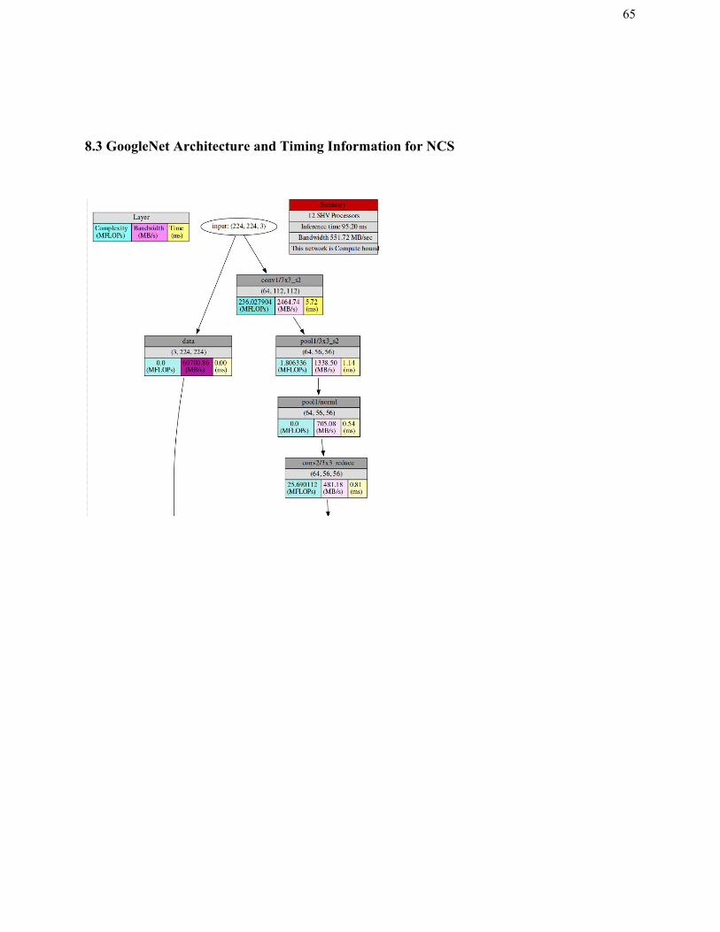
8.3 GoogleNet Architecture and Timing Information for NCS

investigation of deep neural network image processing for

Documents