investigation into the impact of biosurfactant in heavy oil...

i

Investigation into the Impact of Biosurfactant in Heavy

Oil Reservoirs

Sunday Victor Ukwungwu

(B. Eng., M.Sc.)

School of Computing, Science and Engineering

Petroleum Technology and Spray Research Group

University of Salford, Manchester, UK

Supervisors

Dr. A. J. Abbas

Professor G. G. Nasr

Submitted in Partial Fulfilment of the Requirement of the Degree of Doctor of

Philosophy, October 2017

ii

Table of Contents

Table of Contents ..................................................................................................................... ii

List of Tables ........................................................................................................................... ix

List of Figures ........................................................................................................................... x

Acknowledgement ................................................................................................................. xiv

Declaration.............................................................................................................................. xv

Nomenclature ........................................................................................................................ xvi

Conversion Table .................................................................................................................. xix

Publications and Conference ................................................................................................ xx

Abstract .................................................................................................................................. xxi

Chapter 1 .................................................................................................................................. 1

1 Introduction ...................................................................................................................... 1

Chapter 2 .................................................................................................................................. 6

2 Literature Review ............................................................................................................. 6

Chemistry, Structure and Classification of Surfaces active compounds ........... 14

Biosurfactant Producing Microorganisms ......................................................... 16

Biosurfactant in the Petroleum Industry ............................................................ 17

Classification of MEOR ..................................................................................... 18

MEOR mechanism ............................................................................................. 19

iii

Carbon Source .................................................................................................... 21

Nitrogen Source ................................................................................................. 22

Chapter 3 ................................................................................................................................ 31

3 Experimental Apparatus, Materials and Procedure ................................................... 31

Experimental Apparatus and Materials .............................................................. 34

3.2.1.1 Fume cupboard ........................................................................................... 34

3.2.1.2 Eppendorf mastercycler® pro S ................................................................. 34

3.2.1.3 Measurement of the Cell Concentration by Optical Density (OD) ............ 35

3.2.1.4 Growth Media ............................................................................................. 36

3.2.1.5 Microorganism............................................................................................ 36

3.2.1.6 Reference Strains ........................................................................................ 37

Procedure of data collection............................................................................... 37

3.2.2.1 Nutrient Agar-Luria Broth .......................................................................... 37

3.2.2.2 Bacterial strain revival ................................................................................ 38

3.2.2.3 Growth at Different Temperatures ............................................................. 38

3.2.2.4 Stock Solution (Preservation of the Strains) ............................................... 38

3.2.2.5 Determination of Phenotypic Characteristics ............................................. 40

3.2.2.5.1 Colony Morphology of Microorganisms ................................................. 40

3.2.2.5.2 Gram-Staining ......................................................................................... 40

3.2.2.5.3 PCR Amplification .................................................................................. 41

3.2.2.6 Serial Dilution for bacterial strain .............................................................. 43

3.2.2.7 Biosurfactant Extraction Process ................................................................ 44

Error and Accuracy ............................................................................................ 44


iv

3.3.1.1 The TEMCO Pendant Drop ........................................................................ 45

3.3.1.2 The Quizix pump ........................................................................................ 50

3.3.1.3 Fluid Samples ............................................................................................. 51

3.3.1.4 Produced Biosurfactants ............................................................................. 52


3.3.2.1 Dilutions of produced biosurfactants with brine. ....................................... 52

3.3.2.2 Procedure for Interfacial Tension and Contact Angle Measurements ........ 54

3.3.2.3 Filling the system with liquid ..................................................................... 54

3.3.2.4 Pressurizing the IFT cell using the hand pump .......................................... 55

3.3.2.5 Experimental run/IFT measurement ........................................................... 56

3.3.2.6 Cleaning of the IFT Cell ............................................................................. 57

3.3.2.7 Precautions.................................................................................................. 57



3.4.1.1 The Soxhlet Extraction ............................................................................... 59

3.4.1.2 Principle of the Soxhlet extraction method ................................................ 60

3.4.1.3 Rock Samples ............................................................................................. 61


3.4.2.1 The Soxhlet extraction/Core Cleaning ....................................................... 62

3.4.2.2 Core Sample preparation for crude oil treatment ....................................... 63

3.4.2.3 Core Sample Preparation for bio-surfactant treatments ............................. 64

3.4.2.4 Floating test ................................................................................................ 65

3.4.2.5 Two phase separation test ........................................................................... 65



3.5.1.1 Description of CoreLab UFS-200............................................................... 67

3.5.1.2 Core Holder ................................................................................................ 70

3.5.1.3 The Injection System .................................................................................. 71

3.5.1.3.1 Floating-Piston Accumulators ................................................................. 71

3.5.1.3.2 Metering Pump and Overburden Pressure Pump .................................... 73

3.5.1.4 The Collection System................................................................................ 74

3.5.1.5 The Data Acquisition and Control System. ................................................ 75

v

3.5.1.6 Back-Pressure Regulator, Pressure Gauges, Air Actuated Valves, and

Pressure Transducers ...................................................................................................... 75

75

5.5.1.7 Materials ..................................................................................................... 75


76

5.5.2.1 Initial Setup................................................................................................. 76

3.5.2.2 Filling the Floating-Piston Accumulators with Lexan CC Cells ................ 76

3.5.2.3 Inserting Sample in the Core Holder .......................................................... 77

3.5.2.4 Applying Overburden Pressure and Back Pressure .................................... 77

3.5.2.5 Fluid Injection System ................................................................................ 78

3.5.2.5.1 Saturating the sample with formation water ............................................ 79

3.5.2.5.2 Displacing the formation water with crude oil ........................................ 79

3.5.2.5.3 Displacing the crude oil with distilled water (waterflooding) ................. 80

3.5.2.5.4 Displacing the crude oil with bio-surfactant (bioflooding) ..................... 80

3.5.2.6 End Test ...................................................................................................... 80

Errors and Accuracy .......................................................................................... 81

Chapter 4 ................................................................................................................................ 83

4 Result and Discussions ................................................................................................... 83

Culture and Growth............................................................................................ 84

Phenotypic Characteristics ................................................................................. 84

4.2.2.1 Colony Morphology of Microorganisms .................................................... 84

4.2.2.2 Gram Staining ............................................................................................. 88

PCR Amplification............................................................................................. 88

Serial Dilutions .................................................................................................. 88

Measurement of the Cell Concentration by Optical Density (OD) .................... 93

Interfacial Tension Measurements ..................................................................... 94

4.3.1.1 Bacillus subtilis (BS-1) cells ....................................................................... 95

4.3.1.2 Bacillus subtilis (BS-1) cell-free ................................................................. 99

4.3.1.3 Bacillus licheniformis (BS-2) with cells ................................................... 100

vi

4.3.1.4 Bacillus licheniformis (BS-2) cell-free ..................................................... 103

4.3.1.5 Paenibacillus polymyxa (BS-3) Cells ....................................................... 107

4.3.1.6 Paenibacillus polymyxa (BS-3) cell-free .................................................. 108

4.3.1.7 Comparison of IFT with temperature and time for BS-1, BS-2 and BS-3

Biosurfactants with Cells .............................................................................................. 110

4.3.1.8 Comparison of the effect of IFT with temperature for supernatant BS-1, BS-

2 and BS-3 Biosurfactants ............................................................................................ 112

Contact Angle Measurements .......................................................................... 114

4.3.2.1 Film (oil-drop) formation ......................................................................... 116

Floating Test .................................................................................................... 119

Two-phase separation test ................................................................................ 122

Oil Recovery .................................................................................................... 128

Chapter 5 .............................................................................................................................. 134

5 Risk Assessment in Utilising Biosurfactant produced from the Bacillus Genus .... 134

Identification and Overview ............................................................................ 137

Physical/Chemical Properties Assessment ...................................................... 138

Ecological Risk Assessment ............................................................................ 138

Human Health Risk Assessment ...................................................................... 138

Identification and Overview ............................................................................ 142

Human Health Risk Assessment ...................................................................... 143

Ecological Risk Assessment ............................................................................ 143

Biological and ecological properties ................................................................ 147

Effects on the environment .............................................................................. 147

Effects on human health................................................................................... 148

vii

Hazard severity ................................................................................................ 148

Sources of exposure ......................................................................................... 148

Risk Characterization ....................................................................................... 149

Chapter 6 .............................................................................................................................. 154

6 Economic Analysis Using BS-2 Biosurfactant to Enhance Residual Oil in Nembe

field, Niger delta. .................................................................................................................. 154

Total Capital Cost for Drilling the Injection Well ........................................... 155

Estimation of operating expenditure (OPEX) .................................................. 156

6.2.2.1 Preparation of Biosurfactant ..................................................................... 156

Revenue generated from the sales of Oil produced ......................................... 157

Estimation of Depreciation Cost/Tax............................................................... 158

Chapter 7 .............................................................................................................................. 167

Conclusions and Future Works .......................................................................................... 167

References ............................................................................................................................. 170

APPENDICES ...................................................................................................................... 182

ix

List of Tables

Table 2.1: Use of cheap raw materials to produce biosurfactants by various microbial strains

.................................................................................................................................................. 24

Table 3.1: Strains used in this study. ...................................................................................... 37

Table 3.2: Nucleotide sequence of the 16s rRNA gene .......................................................... 42

Table 3.3: Crude-oil Characteristics ....................................................................................... 51

Table 3.4: Composition of formation water ............................................................................ 52

Table 3.5: Density measurements for cultured biosurfactants ................................................ 53

Table 3.6: Core Characterisation ............................................................................................ 61

Table 4.1: Greatest contact angle reduction of all produced biosurfactant ........................... 115

Table 4.2: Wettability effect on sandstone grains after treatment with biosurfactants ......... 122

Table 4.3: Data analysis for recovery factor ......................................................................... 130

Table 5.1: Probability of occurrence ..................................................................................... 140

Table 5.2: Risk rating matrix ................................................................................................ 141

Table 5.3: Planned response (mitigation) ............................................................................. 142







Table 6.1: Typical cost estimate for drilling an injection well ............................................. 156

Table 6.2: Annual operating costs......................................................................................... 157

Table 6.3: Annual sales of oil produced ............................................................................... 158

Table 6.4: Cash flow at 10% discount rate of drilling an injection well ............................... 163

Table 6.5: Cost Summary of Drilling Injection Well............................................................ 165

x

List of Figures

Figure 1.1: Process of microbial recovery of crude oil using biosurfactant ............................. 2

Figure 2.1: Forming a transition zone ....................................................................................... 9

Figure 2.2: Wetting in pores ................................................................................................... 11

Figure 2.3: Surfactant structure of surfactin (C53H93N7O13) ................................................... 14

Figure 2.4: Structure of a (bio/surfactant) molecule ............................................................... 15

Figure 2.5: Surfactant adsorption process at interface ............................................................ 16

Figure 2.6: The basic process of microbial enhanced oil recovery ........................................ 18

Figure 2.7: Cyclic microbial oil recovery ............................................................................... 19

Figure 2.8: Microbial flooding recovery................................................................................. 20

Figure 2.9: Pendant drop method ............................................................................................ 28

Figure 3.1: Structure and sequence of experimental methodology ........................................ 33

Figure 3.2: Retrieving of the selected bacteria strains ............................................................ 34

Figure 3.3: Eppendorf mastercycler® pro S ........................................................................... 35

Figure 3.4: UV spectrophotometer ......................................................................................... 35

Figure 3.5: Liquid nutrient broths ........................................................................................... 36

Figure 3.6: Pouring a plate of nutrient agar ............................................................................ 38

Figure 3.7: Stock solutions of the revived freezed dreid strains ............................................. 39

Figure 3.8: Serial dilution for bacteria strain .......................................................................... 43

Figure 3.9: Schematic illustration of the pendant drop set-up ................................................ 46

Figure 3.10: The complete set-up of the IFT-cell ................................................................... 47

Figure 3.11: Low temperature/high pressure interfacial tension/contact angle cell apparatus

.................................................................................................................................................. 48

Figure 3.12: Pressure transducer/acquisition section .............................................................. 49

Figure 3.13: The Quizix pump ................................................................................................ 50

Figure 3.14: Crude oil and synthetic formation water ............................................................ 51

Figure 3.15: MSM and dilutions of produced biosurfactants for cells and cell-free cultures 54

Figure 3.16: Soxhlet kit .......................................................................................................... 59

Figure 3.17: Heating mantle ................................................................................................... 60

Figure 3.18: Heating Mantle (Temperature) controller .......................................................... 60

Figure 3.19: The soxhlet extraction process ........................................................................... 61

Figure 3.20: Sandstone core plugs .......................................................................................... 62

Figure 3.21: Crushed grains of sizes 300 µm and 225 µm. .................................................... 63

xi

Figure 3.22: Aging of the sandstone cores in crude oil .......................................................... 63

Figure 3.23: Saturation of bandera gray sandstone in BS-1 BS-2 and BS-3 ........................... 64

Figure 3.24: Saturation of scioto sandstone in BS-1 BS-2 and BS-3....................................... 64

Figure 3.25: Floating test (a) oil-wet rock (b) water-wet rock ............................................... 65

Figure 3.26: Two phase separation test (a) oil-wet rock (b) water-wet rock .......................... 66

Figure 3.27: Cross-section of the UFS-200 core flooding equipment. ................................... 68

Figure 3.28: Schematic diagram of the flow path used in the core flooding experiment ....... 69

Figure 3.29: Core holder ......................................................................................................... 70

Figure 3.30: A cross-section of the hassle core holder ........................................................... 71

Figure 3.31: Floating-piston accumulators ............................................................................. 72

Figure 3.32: CC cells .............................................................................................................. 72

Figure 3.33: Metering Isco pumps .......................................................................................... 73

Figure 3.34: Overburden pump and relevant reservoirs ......................................................... 74

Figure 3.35: Hameg electronic balance .................................................................................. 74

Figure 3.36: Adjustable and fixed end plug ............................................................................ 77

Figure 3.37: The fluid Injection process. ................................................................................ 79

Figure 4.1: Isolation of pure cultures and growth of bacteria ................................................. 85

Figure 4.2: Bacteria growth after 48 hours, stores at 30oC. .................................................... 86

Figure 4.3: Bacteria growth after 48 hours, stores at 37oC. .................................................... 87

Figure 4.4: Appearance of gram-positive cells of the selected strains ................................... 90

Figure 4.5: Sequence alignment for the selected strains. ........................................................ 91

Figure 4.6: View of bacteria colonies from Bacillus subtilis at different dilutions................ 92

Figure 4.7: Effect of temperature on IFT for crude oil/distilled water system ....................... 95

Figure 4.8: Experimental of IFT data with temperature for Bacillus subtilis cells ................ 97

Figure 4.9: Pressure effect on IFT for BS-1 cells ................................................................... 98

Figure 4.10: Temperature effect on IFT for BS-1 cell-free biosurfactant. .............................. 99

Figure 4.11: Effect of pressure on IFT for cell-free BS-1-biosurfactant .............................. 100

Figure 4.12: Pressure effect on IFT for BS-2 biosurfactant cells .......................................... 101

Figure 4.13: IFT with temperature at varying pressures for BS-2 with cells. ....................... 102

Figure 4.14: IFT with time for BS-2 biosurfactant at 42oC .................................................. 103

Figure 4.15: Variation of IFT with time for BS-2 biosurfactant at 75oC .............................. 103

Figure 4.16: IFT with temperature at varying pressures for BS-2 biosurfactant cell-free .... 104

Figure 4.17: IFT with time for BS-2 biosurfactant cell-free at 32oC .................................... 106


xii


Figure 4.20: IFT with temperature at varying pressures for BS-3 with cells ........................ 107

Figure 4.21: Pressure effect on IFT for BS-3 cell-free at varying temperatures ................... 108

Figure 4.22: Temperature effect on IFT for BS-3 cell-free at varying pressures. ................. 109

Figure 4.23: Comparison of IFT with temperature for biosurfactants with cells ................. 111

Figure 4.24: Comparison of IFT with temperature for supernantant biosurfactants ............ 113

Figure 4.25: Effect of drop size on contact angle values for different pressures at 75oC ..... 116

Figure 4.26: Film formation of oil with Bacillus subtilis cells biosurfactant at; (a) 26oC, 0.15

MPa (b) 42oC, 0.15 MPa (c) 60oC, 13.89 MPa ...................................................................... 116

Figure 4.27: Film formation of oil with Bacillus licheniformis biosurfactant cells at 0.15

MPa; (a) 26oC, (b) 42oC, (c) 75oC ......................................................................................... 117

Figure 4.28: Film formation of oil with Bacillus subtilis cell-free biosurfactant at; (a) 26oC,

0.15 MPa (b) 42oC, 12.51 MPa (c) 75oC, 10.44 MPa ............................................................ 117

Figure 4.29: Film formation of oil with Bacillus licheniformis cell-free biosurfactant at 3.10

MPa; (a) 26oC, (b) 42oC, (c) 75oC ......................................................................................... 117

Figure 4.30: Film formation of oil with paenibacillus polymyxa cell-free biosurfactant at

10.44 MPa (a) 32oC, (b) 42oC, (c) 75oC ................................................................................ 118

Figure 4.31: Control test for distilled water and untreated grain samples without

biosurfactant (a) Scioto, (b) Bandera gray ............................................................................. 119

Figure 4.32: Distilled water and treated scioto grain sample in biosurfactant with cells ..... 120

Figure 4.33: Distilled water and treated bandera gray grain sample in biosurfactant with cells

................................................................................................................................................ 121

Figure 4.34: Distilled water and treated scioto grain sample in cell-free biosurfactants ...... 121

Figure 4.35: Distilled water and treated bandera gray grain sample in cell-free biosurfactants

................................................................................................................................................ 122

Figure 4.36: Distilled water with kerosene plus treated grain samples in biosurfactants for

both cells and cell-free ........................................................................................................... 123

Figure 4.37: Distilled water with sunflower plus treated grain sample in biosurfactant with

cells ........................................................................................................................................ 124

Figure 4.38: Distilled water with sunflower plus treated grain sample in cell-free

biosurfactants. ........................................................................................................................ 124

Figure 4.39: Distilled water flooding versus time ................................................................ 127

Figure 4.40: Biosurfactant flooding versus time. ................................................................. 127

xiii

Figure 4.41: Differential pressure across the sample versus time for the water flooding cycle

................................................................................................................................................ 128

Figure 4.42: Differential pressure across the sample versus time for the biosurfactant

flooding cycle......................................................................................................................... 129

Figure 4.43: Oil recovery curves with injected pore volumes .............................................. 131

Figure 4.44: Comparison between surfactant solutions in residual oil recovery .................. 132

Figure 5.1: Stages of risk assessment ................................................................................... 135

Figure 5.2: Adopted 3 × 3 impact matrix.............................................................................. 137

Figure 5.3: Probability impact grid ....................................................................................... 141



Figure 6.1: Cooperate cash flow diagram ............................................................................. 160

Figure 6.2: Payback period for drilling the injection well .................................................... 164

Figure 6.3: Break-even graph of enhanced recovery using BS-2 biosurfactant .................... 166

xiv

Acknowledgement

With gratitude in my heart, I thank God for bringing me this far to successfully complete this

dream despite all odds. And to my wonderful parents, who have always been the source of

my inspiration, I cannot thank you enough for how much you invested in my education; you

are truly the world’s best anyone would wish for. May the good Lord continue to bless you

and grant you long life. To my supervisors, Dr. A. J. Abbas and Prof. Nasr, I sincerely

appreciate your support, encouragements and guidance during my research study. It was a

good experience working with you.

To my lecturers and staff, Dr. Enyi, Dr. Burby, and Mr Alan Mappin, I appreciate all the

help, advice and academic support especially during my laboratory experimental work. And

to all my colleagues in the Petroleum and Spray Research Group, I want to say big thank you

for being part of my success story, it was a lot of fun working with you and knowing you.

And a special thanks to, Dr. Heather Allison and Sean Goodman, from the department of

Functional and Comparative Genomics, Institute of Integrative Biology, University of

Liverpool, for their support in carrying out the phase I of this study.

I appreciate my dearest siblings and especially my twin, for your prayers, love, and the trust

you have in me. You guys are just the best siblings I could ever have wished for, even with

miles apart, you all are always close to my heart. I will sure make you and our family proud

for believing so much in me. Thank you for your prayers; it gave me so much grace to

journey smoothly through my lowest moments.

To my darling wife, my jewel of inestimable value, my ever-smiling wife, I thank you for

your patience, love and endurance throughout my research study; you have and will always

be my pillar and source of strength. Thank you for bearing forth our little angel and daughter

and for caring for her while I studied, you both are everything I work and live for. May God

bless and keep you both. Now that I have completed my studies, I will surely make up for all

the times I was unavoidably absent at home.

Finally, to all my friends and relatives who have always been there to support and encourage

me when I needed it the most, may God bless you and reward you for your kindness. I give

special thanks to Esosa, Chika, Oge, Ifeanyi, Isaac, Kevin, Emeka, Francis, Busayo, Ebimor,

Lucky; you guys have always looked out for me.

xv

Declaration

I Ukwungwu Sunday Victor, declare that this thesis report is my original work, and has not

been submitted elsewhere for any award. Any section, part or phrasing that has been used or

copied from other literature or documents copied has been clearly referenced at the point of

use as well as in the reference section of this thesis.

…………………………. ……………………..

Signature Date

……………………… …………………

Approved by

Prof. G. G. Nasr

Dr A. J. Abbas (Supervisor)

(Supervisor)

xvi

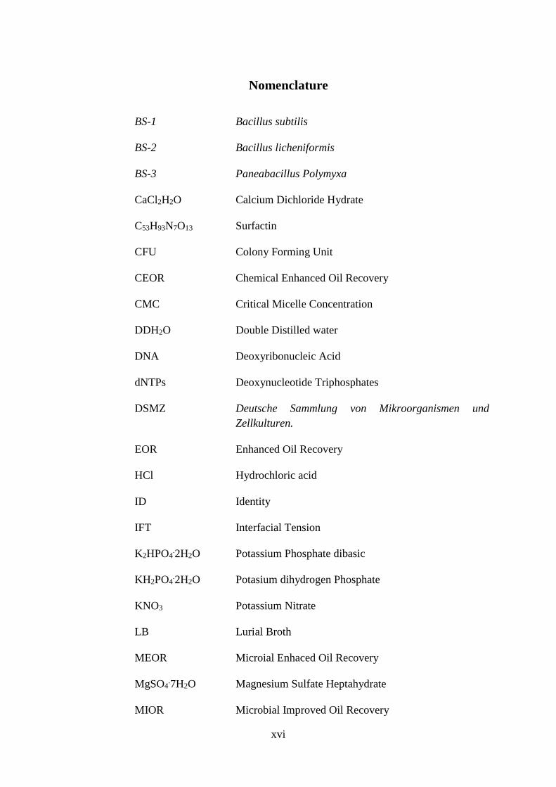
Nomenclature

BS-1 Bacillus subtilis

BS-2 Bacillus licheniformis

BS-3 Paneabacillus Polymyxa

CaCl2H2O Calcium Dichloride Hydrate

C53H93N7O13 Surfactin

CFU Colony Forming Unit

CEOR Chemical Enhanced Oil Recovery

CMC Critical Micelle Concentration

DDH2O Double Distilled water

DNA Deoxyribonucleic Acid

dNTPs Deoxynucleotide Triphosphates

DSMZ Deutsche Sammlung von Mikroorganismen und

Zellkulturen.

EOR Enhanced Oil Recovery

HCl Hydrochloric acid

ID Identity

IFT Interfacial Tension

K2HPO4.2H2O Potassium Phosphate dibasic

KH2PO4.2H2O Potasium dihydrogen Phosphate

KNO3 Potassium Nitrate

LB Lurial Broth

MEOR Microial Enhaced Oil Recovery

MgSO4.7H2O Magnesium Sulfate Heptahydrate

MIOR Microbial Improved Oil Recovery

xvii

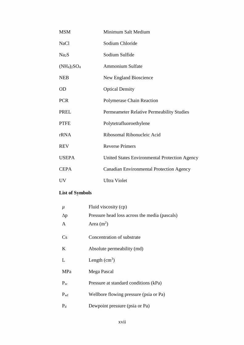
MSM Minimum Salt Medium

NaCl Sodium Chloride

Na2S Sodium Sulfide

(NH4)2SO4 Ammonium Sulfate

NEB New England Bioscience

OD Optical Density

PCR Polymerase Chain Reaction

PREL Permeameter Relative Permeability Studies

PTFE Polytetrafluoroethylene

rRNA Ribosomal Ribonucleic Acid

REV Reverse Primers

USEPA United States Environmental Protection Agency

CEPA Canadian Environmental Protection Agency

UV Ultra Violet

List of Symbols

µ Fluid viscosity (cp)

∆p Pressure head loss across the media (pascals)

A Area (m2)

Cs Concentration of substrate

K Absolute permeability (md)

L Length (cm3)

MPa Mega Pascal

Psc Pressure at standard conditions (kPa)

Pwf Wellbore flowing pressure (psia or Pa)

Pd Dewpoint pressure (psia or Pa)

xviii

Q Volumetric flow rate (Mscfd)

Tsc Temperature at standard conditions (K)

V Volume (m3/s)

xix

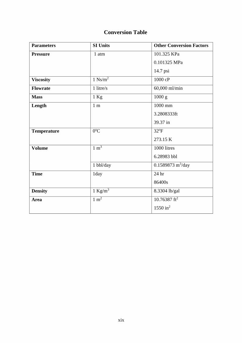
Conversion Table

Parameters SI Units Other Conversion Factors

Pressure 1 atm

101.325 KPa

0.101325 MPa

14.7 psi

Viscosity 1 Ns/m2 1000 cP

Flowrate 1 litre/s 60,000 ml/min

Mass 1 Kg 1000 g

Length 1 m 1000 mm

3.2808333ft

39.37 in

Temperature 0oC 32oF

273.15 K

Volume 1 m3

1000 litres

6.28983 bbl

1 bbl/day 0.1589873 m3/day

Time 1day 24 hr

86400s

Density 1 Kg/m3 8.3304 lb/gal

Area 1 m2 10.76387 ft2

1550 in2

xx

Publications and Conference

1. Ukwungwu, S.V., Abbas, A.J. and Nasr, G.G., 2016. Experimental investigation of

the impact of biosurfactants on residual-oil recovery. 18th International Conference

on Biological Ecosystems and Ecological Networks, Madrid, Spain, 24 - 25 March

2016.


the impact of biosurfactants on residual-oil recovery. International Journal of

Biological, Biomolecular, Agricultural, Food and Biotechnological

Engineering, 10(3), pp.130-133.

3. Ukwungwu, S.V., Abbas, A.J. and Nasr, G.G., Allison, H., Goodman, S., 2017.

Wettability Effects on Bandera Gray Sandstone using Biosurfactants. Journal of

Engineering Technology. Volume 6, Issue 2, July, 2017, PP.605-617.

(See Appendix A)

xxi

Abstract

Exploitation of oil resources in mature reservoirs is essential for meeting future energy

demands. Despite the primary and secondary oil recovery, significant amount of residual oil

is still left behind in the reservoir, necessitating tertiary recovery methods. These typically

includes surfactant flooding, polymer flooding, Microbial Enhanced Oil Recovery (MEOR)

etc. To exemplify the potential of microorganisms to degrade heavy crude oil to reduce its

viscosity, is part of a process known as MEOR. In recent times surfactants produced by

microbes have gained wider acceptability in the petroleum industry due to their low toxicity

and ease with which they are naturally broken down in the environment. Petrochemical-based

synthetic surfactants are currently used in substantial amounts to increase recovery of

hydrocarbons, and these surfactants are more recalcitrant in the environment.

The present study therefore, uses a technique to utilise microbes that will economically

achieve a scale of Enhanced Oil Recovery (EOR) through biosurfactant production, lowering

of interfacial tension (IFT) and contact angle, changes in rock wettability of sandstone grains

and biosurfactant flooding. Three biosurfactants were produced under laboratory conditions,

from three species of the genus bacillus using sucrose 3% (w/v) as their carbon source for

growth and metabolism. These species produced biosurfactants of different specific activities

that resulted in different impacts on IFT and contact angle. The biosurfactants produced are

BS-1, BS-2 & BS-3. After applying the cell-free extracellular biosurfactants to the system, the

results show that there is reduction in interfacial tension from 56.95 mN/m to 4.49 mN/m,

6.69 mN/m, and 10.94 mN/m. Also, the contact angle of the oil film was significantly

reduced from 147.04° to 111.84o, when the cell-free extracellular biosurfactant (BS-2) was

applied to the system.

Qualitative wettability tests were also performed on the sandstone crushed rock samples,

which shows that, the spent culture medium changes wettability of the grains to water-wet

and intermediate-wet. It should be noted that the decomposition property of sucrose as a

carbon source makes it eco-friendly for biosurfactant production. The biosurfactant flooding

also found to have a recovery of 38% (an interval of nominally 8%) against 30% water

flooding, due to the development of a water-wet state, which was achieved by flooding the

core with 5PV of BS-2 supernatant solution.

xxii

Economic analysis was also considered in determining the possible profitability of the

corresponding MEOR method with addition of biosurfactant costs that were utilised during

this study. The case study results of these analysis show that the cumulative cashflow,

indicated a payback period of 2.54 years for a capital investment of $45.32 million, given a

typical oil production of 2,720 barrel per day. Moreover, with this type of biosurfactant (BS-

2) supernatant, it has become evident that there can be an enhance recovery in the heavy oil

reservoir by changing the wettability of rock grains. This thus, provides new tools for use in

EOR schemes that leads to promising environmental sustainability.

1

Chapter 1

1 Introduction

Exploitation of oil resources in mature reservoirs is an essential task for meeting the current

and future energy demands. Advances in petroleum biotechnology in recent years has been

driven by the growing global demand for sustainable technologies, that improves the

efficiency of petrochemical processes in the oil industry (De Almeida et al., 2016), as well as

providing promising schemes for oil recovery. An important tertiary oil recovery technique is

Microbial Enhanced Oil Recovery (MEOR) which is an eco-friendly technology and cost-

effective alternative (Banat et al., 2010) to both thermal and chemical enhanced oil recovery

methods, in which microbes or their metabolic products are used to drive the residual oil

trapped in the reservoirs (de Lima & de Souzaa, 2014; Filho, Carioca, Gonzales, de Lucena,

& Tavares, 2012; S. Johnson, Salehi, Eisert, & Fox, 2009). The potential of microorganisms

to produce sufficient biosurfactants, starting with low-cost substrates raw materials is mainly

to degrade heavy crude oil to reduce viscosity and improve hydrocarbon mobilization. This is

considered to be very effective in enhancing crude oil recovery from reservoirs (Sarafzadeh

et al., 2014; Silva et al., 2014). Since thermophilic spore-forming bacteria can thrive in very

extreme conditions in oil reservoirs (up to 80oC), they are the most suitable organisms for this

purpose (Nicholson, Munakata, Horneck, Melosh, & Setlow, 2000; Shibulal et al., 2014).

Surfactants of microbial origin in the last decade have become of great interest because of

their advantages over their chemical counterparts, which include low toxicity,

biodegradability, effectiveness in adverse environmental conditions, ability to produce from

renewable resources and environmental compatibility (Filho et al., 2012). These benefits of

metabolic products can be explored in solving many problems often encountered during oil

production in respect to improving the recovery of crude oil from reservoir rocks (Lazar,

Petrisor, & Yen, 2007). It is therefore very necessary to protect the environment by utilizing

microbial flooding technique for EOR processes, and the products of microbial fermentation

of carbohydrates. The fundamental cause for leaving oil behind is economics. In general, the

process of recovering oil from any conventional reservoir requires firstly, a pathway which

connects oil in the pore spaces of a reservoir to the surface, and secondly, sufficient energy in

the reservoir to drive the oil to the surface. Lack of these inter-linked requirements in a

reservoir results in oil getting left behind (Springham, 1984). The varying permeability of

petroleum reservoirs is also a major concern in EOR processes. It is important to know that

2

the chemicals used for EOR must be compatible with the physical and chemical

environments of oil reservoirs.

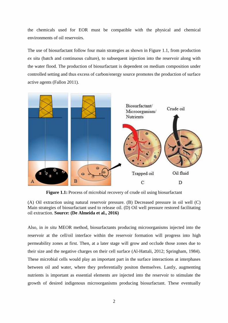
The use of biosurfactant follow four main strategies as shown in Figure 1.1, from production

ex situ (batch and continuous culture), to subsequent injection into the reservoir along with

the water flood. The production of biosurfactant is dependent on medium composition under

controlled setting and thus excess of carbon/energy source promotes the production of surface

active agents (Fallon 2011).

Figure 1.1: Process of microbial recovery of crude oil using biosurfactant

(A) Oil extraction using natural reservoir pressure. (B) Decreased pressure in oil well (C)

Main strategies of biosurfactant used to release oil. (D) Oil well pressure restored facilitating

oil extraction. Source: (De Almeida et al., 2016)

Also, in in situ MEOR method, biosurfactants producing microorganisms injected into the

reservoir at the cell/oil interface within the reservoir formation will progress into high

permeability zones at first. Then, at a later stage will grow and occlude those zones due to

their size and the negative charges on their cell surface (Al-Hattali, 2012; Springham, 1984).

These microbial cells would play an important part in the surface interactions at interphases

between oil and water, where they preferentially positon themselves. Lastly, augmenting

nutrients is important as essential elements are injected into the reservoir to stimulate the

growth of desired indigenous microorganisms producing biosurfactant. These eventually

3

helps to increase the sweep efficiency, and thus a more efficient oil transport can be achieved

(Al-Bahry et al., 2013; Bachmann, Johnson, & Edyvean, 2014).

On a fundamental level, the process of MEOR results in beneficial effects such as formation

of stable oil-water emulsions, reduced interfacial tension/capillary forces, clogging the high

permeable zones and the breakdown of the oil film in the rocks which are important for

maximizing and extending the reservoir life time (Al-Bahry et al., 2013; Bachmann et al.,

2014).

Oil advancement through porous media is expedited by modifying the interfacial properties

of the oil-water minerals. In such a system, microbial activity alters fluidity (viscosity

reduction, miscible flooding); displacement efficiency (decrease of interfacial tension,

increase of permeability); sweep efficiency (mobility control, selective plugging); and driving

force (reservoir pressure). The second principle is known as upgrading. In this case, the

degradation of heavy oils into lighter ones occurs by microbial activity. Instead, it can also

aid in the removal of sulphur from heavy oils as well as the removal of heavy metals (H. Al-

Sulaimani et al., 2011; Sen, 2008; Vazquez-Duhalt & Quintero-Ramirez, 2004).

Microorganisms can synthesize useful products by fermenting low-cost substrates or raw

materials. Therefore, MEOR can substitute Chemical Enhanced Oil Recovery (CEOR),

which is a very pricey technology (Banat et al., 2010; Lazar et al., 2007). In MEOR, the

chosen microbial strains are used to synthesize compounds analogous to those used in CEOR

processes, to increase the recovery of oil from depleted and marginal reservoirs.

1.1 Problem Statement

Environmental impacts, surfactant cost and oil price are the three main parameters that have

effect on the robustness of the surfactant flooding in oil reservoirs. Interfacial tension

reduction and wettability alteration of the reservoir rocks are the two-main mechanism of oil

recovery by utilizing surfactant flooding. There are a number of methods used to improve

well productivity by earlier studies of MEOR (Davis & Updegraff, 1954; Kuznetsov, 1950;

Updegraff & Wren, 1954) were based on three broad areas: injection, dispersion, and

propagation of microorganisms in petroleum reservoirs; selective degradation of oil

components to improve flow characteristics; and production of metabolites by

microorganisms and their effects (Shibulal et al., 2014).

4

Great emphasis has been given to the ecological effects (Dusseault, 2001; Ivanković &

Hrenović, 2010; Venhuis & Mehrvar, 2004; Ying, 2006) caused by chemical surfactants due

to their toxicity and difficulty of degrading in the environment. Increasing ecological

concerns, development in biotechnology, and the rise of more stringent environmental laws

have prompted biosurfactants being a potential option to the synthetic surfactants available in

the market. For as long as oil production will continue, the adoption of an environmentally

friendly technique for enhancing effective oil recovery must be considered. Specifically, this

study is focused on the following aspects:

Environmental impact: addressing the adverse effects of CEOR on the eco-system,

this study utilises thermophilic spore-forming bacteria to grow on a carbohydrate

substrate which are easily degradable.

Producing schemes: different producing schemes may affect the composition structure

between the values of flowing and static properties and the amount of trapped oil in

the reservoir, which may in turn influence the well productivity and hence the

ultimate oil recovery from the reservoir. Changing the wettability of the rock and the

manner in which the well is brought into flowing condition can affect the pore spaces

and subsequently prolong the life of mature fields.

1.2 Contribution to research

Utilisation of biosurfactants through re-generation and characterisation of related species,

leading to optimisation of the ultimate oil transport and enhancing oil recovery.

1.3 Aim

To develop a technique for MEOR in heavy oil reservoirs to effectively transport residual oil

left behind and economically beneficial, when compared to other conventional techniques.

1.4 Objectives

1. To isolate pure culture and investigate the strain of bacteria that can be effectively

used to produce the required biosurfactant through the addition of LB broth and

culturing on LB agar plates.

2. To investigate surface reaction of these biosurfactants in reducing the interfacial

tension and contact angle of heavy oil.

5

3. To investigate changes in wettability for different types of rocks and for a variety of

biosurfactants using the qualitative wettability tests.

4. To investigate biosurfactants that can change formation wettability by measuring

unsteady-state relative permeability before and after biosurfactant treatments through

core flooding.

5. To develop an economic evaluation for the MEOR project.

1.5 Thesis Outline

This thesis is arranged in part structures, with each section providing the set of information

and actions carried out as contained in the study as follows;

Chapter 2: This chapter presents a literature review on the role of biosurfactants in

enhancing oil recovery as well as laboratory and field projects of MEOR. The chapter

includes existing techniques on oil and gas recovery, and other associated issues on flow

behaviour are discussed.

Chapter 3: In this chapter, the description of the experimental procedure for producing

biosurfactant using the spread plate technique in culturing the bacteria species was outlined.

Biosurfactant screening for reduction in interfacial tension, brief description of the IFT

measurement equipment by TEMCO and a description of the IFT software/procedure were

also presented. Two methods for qualitative wettability tests were also discussed and a

description of the UFS-200 core flooding equipment.

Chapter 4: This chapter discusses the analysis and outcome of the laboratory investigations

that proved a positive approach to enhancing oil recovery while comparing with relevant

literatures.

Chapter 5: The environmental risk analysis was evaluated for all three produced

biosurfactant, for any possible treats of the microbes to the environment.

Chapter 6: The economic viability of the experimental outcome was considered, if the

project were to be escalated into actual field project.

Chapter 7: This chapter give the conclusion of the entire thesis and future works that could

be further researched into.

6

Chapter 2

2 Literature Review

2.1 Significance of Enhanced Oil Recovery

To meet the global demand for energy consumption, it has become imperative to increase oil

reserve through Enhanced Oil Recovery (EOR). A good understanding and definition of oil

reserves must be determined to obtain what the life of a hydrocarbon reservoir is, since

natural depletion (primary recovery) of a reservoir allows very limited recovery of the oil in

place (Hammershaimb, Kuuskraa, & Stosur, 1983). Reserves refer to the amount of oil that

can be produced from a reservoir under existing economics and with available technology,

which is given by the following material balance equation in Eqn (2.1).

𝑃𝑟𝑒𝑠𝑒𝑛𝑡 𝑟𝑒𝑠𝑒𝑟𝑣𝑒 = 𝑃𝑎𝑠𝑡 𝑟𝑒𝑠𝑒𝑟𝑣𝑒 + 𝐴𝑑𝑑𝑖𝑡𝑖𝑜𝑛𝑎𝑙 𝑟𝑒𝑠𝑒𝑟𝑣𝑒

− 𝑃𝑟𝑜𝑑𝑢𝑐𝑡𝑖𝑜𝑛 𝑟𝑒𝑠𝑒𝑟𝑣𝑒 (2.1)

With the current increase in demand for energy consumption (Miller & Sorrell, 2014; R.

Santos, Loh, Bannwart, & Trevisan, 2014), it has become necessary to either maintain oil

reserves by implementing new techniques to increase the percentage of recovery from

existing reservoirs, drill new wells or discover new fields, to meet this demand. However, the

likelihood of discovering large fields is declining (Michael J McInerney, Nagle, & Knapp,

2005; Muggeridge et al., 2014; Sun, Zhang, Chen, & Gai, 2017), and this has encouraged the

need to increase the percentage of recovery from known reserves with the practical solution

through the application of EOR methods.

2.2 Factors Influencing remaining oil Saturation

EOR implies a reduction of the remaining oil saturation. There are three major factors which

influences the remaining oil saturation in a reservoir. The first factor is the capillary number

(Nc), which affects the pore level oil displacement (Alvarado & Manrique, 2010), and it’s

defined as the ratio of the viscous forces to surface or interfacial tension forces, denoted as;

𝑁𝑐 =µ × 𝑣

𝜎 𝐶𝑜𝑠𝜃 (2.2)

7

Where; v, is the Darcy velocity (m/s), 𝜇 the displacing fluid viscosity (Pa. s), 𝜎, the interfacial

tension (IFT) (mN/m) and θ, is the contact angle.

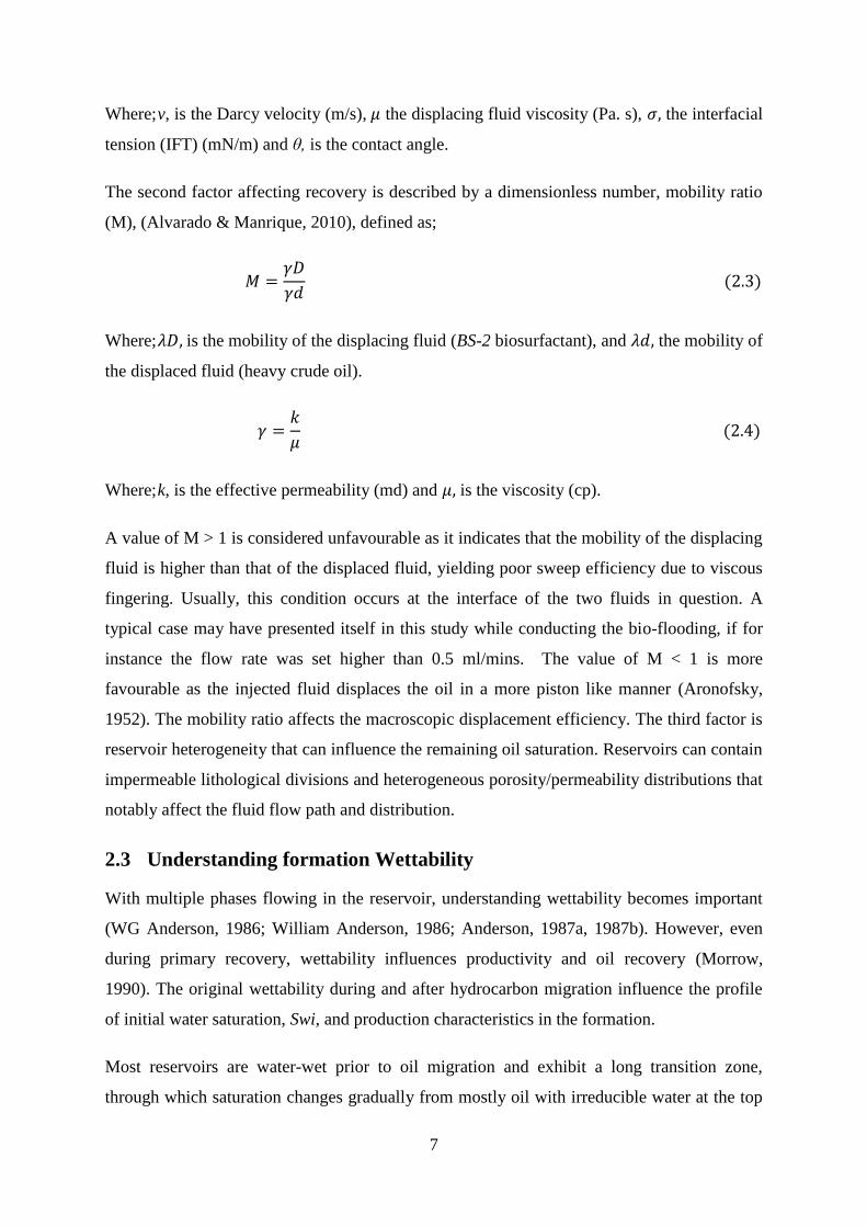
The second factor affecting recovery is described by a dimensionless number, mobility ratio

(M), (Alvarado & Manrique, 2010), defined as;

𝑀 =𝛾𝐷

𝛾𝑑 (2.3)

Where; 𝜆𝐷, is the mobility of the displacing fluid (BS-2 biosurfactant), and 𝜆𝑑, the mobility of

the displaced fluid (heavy crude oil).

𝛾 =𝑘

𝜇 (2.4)

Where; k, is the effective permeability (md) and 𝜇, is the viscosity (cp).

A value of M > 1 is considered unfavourable as it indicates that the mobility of the displacing

fluid is higher than that of the displaced fluid, yielding poor sweep efficiency due to viscous

fingering. Usually, this condition occurs at the interface of the two fluids in question. A

typical case may have presented itself in this study while conducting the bio-flooding, if for

instance the flow rate was set higher than 0.5 ml/mins. The value of M < 1 is more

favourable as the injected fluid displaces the oil in a more piston like manner (Aronofsky,

1952). The mobility ratio affects the macroscopic displacement efficiency. The third factor is

reservoir heterogeneity that can influence the remaining oil saturation. Reservoirs can contain

impermeable lithological divisions and heterogeneous porosity/permeability distributions that

notably affect the fluid flow path and distribution.

2.3 Understanding formation Wettability

With multiple phases flowing in the reservoir, understanding wettability becomes important

(WG Anderson, 1986; William Anderson, 1986; Anderson, 1987a, 1987b). However, even

during primary recovery, wettability influences productivity and oil recovery (Morrow,

1990). The original wettability during and after hydrocarbon migration influence the profile

of initial water saturation, Swi, and production characteristics in the formation.

Most reservoirs are water-wet prior to oil migration and exhibit a long transition zone,

through which saturation changes gradually from mostly oil with irreducible water at the top

8

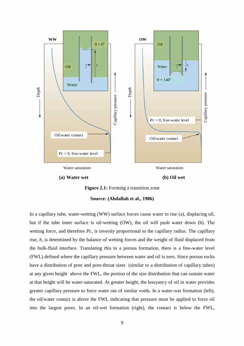
of the transition zone to water at the bottom. This distribution is determined by the bouyancy-

based pressure, Pc as seen in Figure 2.1. Oil migrating into an oil-wet reservoir would

display a different saturation profile: essentially maximum oil saturation down to the base of

the reservoir. This difference reflects the ease of invasion by a wetting fluid. Wettability also

affects the amount of oil that can be produced at the pore level, as measured after waterflood

by the residual oil saturatio (Sor). In a water-wet formation, oil remains in the larger pores,

where it can snap off, or become disconnected from a continous mass of oil, and become

trapped. In an oil-wet or mixed-wet formation, oil adheres to surfaces, increasing the

probability of a contionus path to a producing well and resulting in a lower Sor (Abdallah et

al., 1986).

A homogenious formation exhibits a zone of transition from high oil saturation at the top to

high water saturation at the botton (blue curves). This saturation transition has its origin in the

capillary pressure, Pc, which is the difference between the water and oil pressures at the

interface (Figure 2.1).

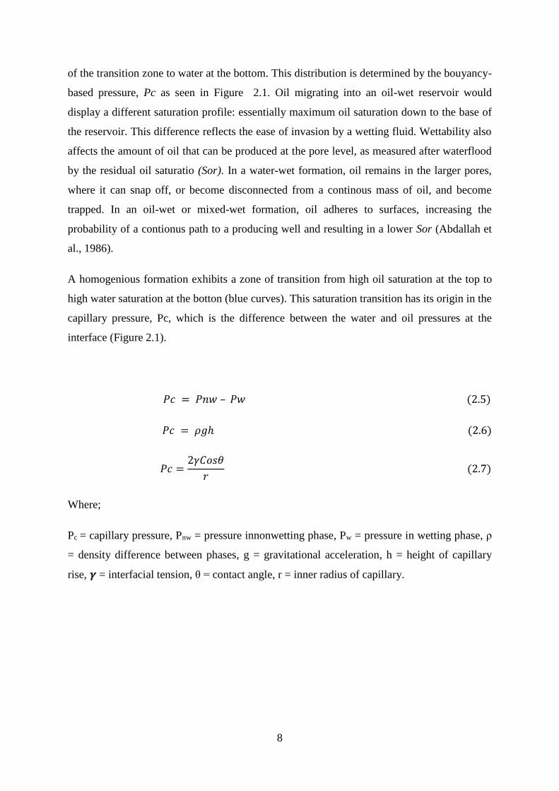
𝑃𝑐 = 𝑃𝑛𝑤 – 𝑃𝑤 (2.5)

𝑃𝑐 = 𝜌𝑔ℎ (2.6)

𝑃𝑐 =2𝛾𝐶𝑜𝑠𝜃

𝑟 (2.7)

Where;

Pc = capillary pressure, Pnw = pressure innonwetting phase, Pw = pressure in wetting phase, ρ

= density difference between phases, g = gravitational acceleration, h = height of capillary

rise, 𝜸 = interfacial tension, θ = contact angle, r = inner radius of capillary.

9

Water saturation Water saturation

Cap

illa

ry p

ress

ure

Cap

illa

ry p

ress

ure

Oil/water contact

Dep

th

Dep

th

Water

Water

θ = 140o

Pc = 0, free-water level

Pc = 0, free-water level

Oil/water contact

WW OW

Oil

Oil

θ = 0o

(a) Water wet (b) Oil wet

Figure 2.1: Forming a transition zone

Source: (Abdallah et al., 1986)

In a capillary tube, water-wetting (WW) surface forces cause water to rise (a), displacing oil,

but if the tube inner surface is oil-wetting (OW), the oil will push water down (b). The

wetting force, and therefore Pc, is inversly proportional to the capillary radius. The capillary

rise, h, is determined by the balance of wetting forces and the weight of fluid displaced from

the bulk-fluid interface. Translating this to a porous formation, there is a free-water level

(FWL) defined where the capillary pressure between water and oil is zero. Since porous rocks

have a distribution of pore and pore-throat sizes (similar to a distribution of capillary tubes)

at any given height above the FWL, the portion of the size distribution that can sustain water

at that height will be water-saturated. At greater height, the bouyancy of oil in water provides

greater capillary pressure to force water out of similar voids. In a water-wet formation (left),

the oil/water contact is above the FWL indicating that pressure must be applied to force oil

into the largest pores. In an oil-wet formation (right), the contact is below the FWL,

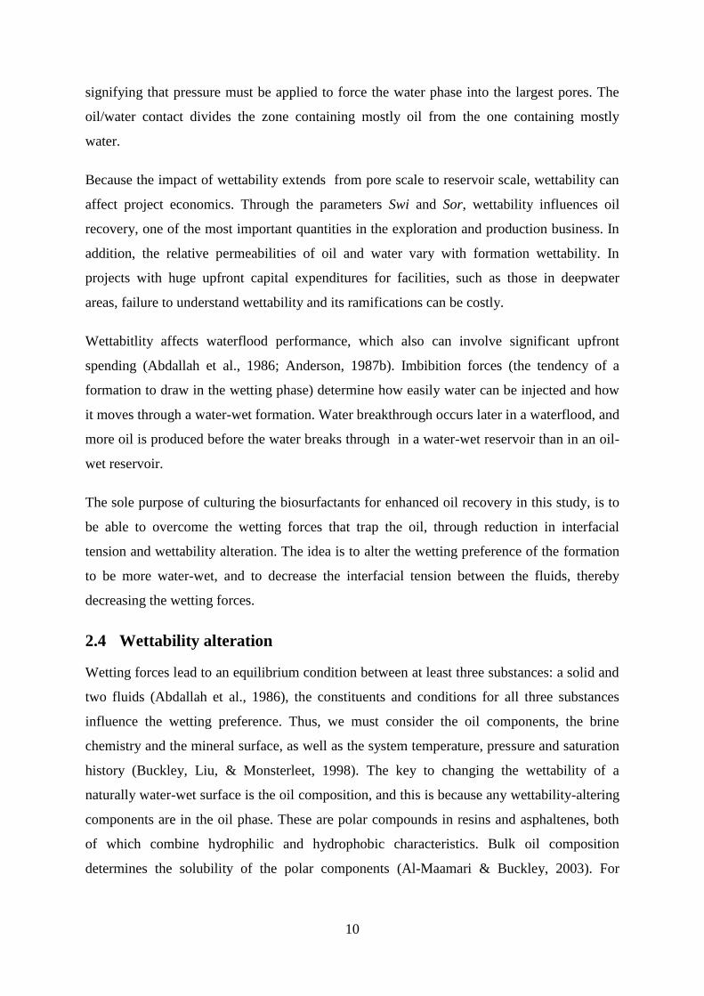
10

signifying that pressure must be applied to force the water phase into the largest pores. The

oil/water contact divides the zone containing mostly oil from the one containing mostly

water.

Because the impact of wettability extends from pore scale to reservoir scale, wettability can

affect project economics. Through the parameters Swi and Sor, wettability influences oil

recovery, one of the most important quantities in the exploration and production business. In

addition, the relative permeabilities of oil and water vary with formation wettability. In

projects with huge upfront capital expenditures for facilities, such as those in deepwater

areas, failure to understand wettability and its ramifications can be costly.

Wettabitlity affects waterflood performance, which also can involve significant upfront

spending (Abdallah et al., 1986; Anderson, 1987b). Imbibition forces (the tendency of a

formation to draw in the wetting phase) determine how easily water can be injected and how

it moves through a water-wet formation. Water breakthrough occurs later in a waterflood, and

more oil is produced before the water breaks through in a water-wet reservoir than in an oil-

wet reservoir.

The sole purpose of culturing the biosurfactants for enhanced oil recovery in this study, is to

be able to overcome the wetting forces that trap the oil, through reduction in interfacial

tension and wettability alteration. The idea is to alter the wetting preference of the formation

to be more water-wet, and to decrease the interfacial tension between the fluids, thereby

decreasing the wetting forces.

2.4 Wettability alteration

Wetting forces lead to an equilibrium condition between at least three substances: a solid and

two fluids (Abdallah et al., 1986), the constituents and conditions for all three substances

influence the wetting preference. Thus, we must consider the oil components, the brine

chemistry and the mineral surface, as well as the system temperature, pressure and saturation

history (Buckley, Liu, & Monsterleet, 1998). The key to changing the wettability of a

naturally water-wet surface is the oil composition, and this is because any wettability-altering

components are in the oil phase. These are polar compounds in resins and asphaltenes, both

of which combine hydrophilic and hydrophobic characteristics. Bulk oil composition

determines the solubility of the polar components (Al-Maamari & Buckley, 2003). For

11

components of an oil to alter wetting, the oil phase must displace brine from the surface. The

surface of a water-wet material is coated by a film of the water phase (Hirasaki, 1991).

2.5 A pore level view

The application of the wetting principles discussed above is complicated by pore geometry.

Understanding a contact angle is easiest when the surface is a smooth plane. However, pore

walls are not smooth, flat surfaces, and typically, more than one mineral species composes

the matrix surrounding the pores. In reality, the complex geometry of a pore is defined by the

grain surfaces surrounding it. The capillary entry pressure in this geometry relates to the

inscribed radius of the largest adjacent pore throat. Although most of the pore body may fill

with oil, the interstices where the grains meet is insufficient to force the non-wetting oil phase

into those spaces (Abdallah et al., 1986).

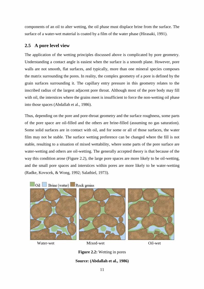
Thus, depending on the pore and pore-throat geometry and the surface roughness, some parts

of the pore space are oil-filled and the others are brine-filled (assuming no gas saturation).

Some solid surfaces are in contact with oil, and for some or all of those surfaces, the water

film may not be stable. The surface wetting preference can be changed where the fill is not

stable, resulting to a situation of mixed wettability, where some parts of the pore surface are

water-wetting and others are oil-wetting. The generally accepted theory is that because of the

way this condition arose (Figure 2.2), the large pore spaces are more likely to be oil-wetting,

and the small pore spaces and interstices within pores are more likely to be water-wetting

(Radke, Kovscek, & Wong, 1992; Salathiel, 1973).

Water-wet Mixed-wet Oil-wet

Figure 2.2: Wetting in pores

Source: (Abdallah et al., 1986)

12

2.6 Wetting in porous media

For any alteration of core wettability, the initially brine-saturated cores are flooded with

crude oil to establish an initial water saturation and an initial measurement of the oil

permeability is made. The value of initial water saturation, aging time, and aging temperature

are the main variables assiociated with the extent of wetting alteration at this stage.

Darcy’s Law describes the relationship between pressure head loss and flow rate in a

homogenous porous media saturated with a monophasic fluid, which is moving through it

(Dake, 2001). In the absence of gravity and for a linear geometry, fluid flow rates depend on:

The geometry of the system; area (A) and Length (L)

Fluid viscosity (µ)

Pressure head loss across the media (∆p)

Experiments have shown that, other variables remaining constant, rate (Q) is proportional to

A and ∆p and inversely proportional to µ and L.

Thus;

𝑄 =𝑘𝐴∆𝑃

𝜇𝐿 (2.8)

2.7 The use of biosurfactant in microbial enhanced oil recovery

In numerous parts of the world for example the North Sea, Mexico, Angola, Brazil, etc., oil

production has been experiencing decline because of oil field development. The increasing

high price of crude oil with attendant increase in demand on world markets and the difficulty

in discovering new oil fields as an alternative to the exploited oil fields in recent years has

contributed to oil decline. Roughly, around 67% of the aggregate petroleum reservoirs in the

world are made up of residual oil, which speaks of the relative inefficiency of the primary

and secondary production methods. A large amount of residual crude oil in depleted

reservoirs can be recovered using MEOR method since the current extraction technique

leaves behind about two-third of the original oil in place. This low cost working technology

can be used to extract about half the leftover residual oil by utilizing microorganisms to haul

out the remaining oil from the reservoirs (Shibulal et al., 2014). In in situ MEOR technique,

microorganisms inoculated with water are injected into the well and at first will advance into

13

high permeability zones, which takes close to a fortnight to do their job. The permeable

medium of reservoir rock is a natural habitat for microorganisms. The organisms then grow

and occlude those zones at a later stage because of their size and the negative charge on their

cell surface (Al-Hattali, 2012). This is accomplished by these organisms producing carbon

dioxide and methane, gases that enter the pores, actively working at the oil-water interface to

possibly squeeze out every ounce of oil. These microorganisms likewise produce

biosurfactants that decrease the tension between oil and the rock surface, which help to

release the oil. The chemical reaction of these microorganisms in oil releases alcohol and

volatile fatty acids. The alcohol reduces the viscosity of the heavy oil, making it sufficiently

light enough to flow out. The fatty acids solubilize the rock surface and in this way push oil

off them. These alterations of the physical and chemical properties of reservoir rocks and

crude oil, extends an opportunity to reverse the declining pattern of oil production by

increasing the sweep efficiency and possibly maintain a curve with a positive slope (Rebecca

S. Bryant & Burchfield, 1989).

2.8 Surfactant and Biosurfactant

The use of organic substrates for biological oil recovery is considered as a more favourable

method than other physical and chemical methods. The amphipathic nature (short chain fatty

acids) of surfactant compounds enables it to have both the polar and non-polar sides, which

enables them to interact with two phases of immiscible emulsions. On an industrial scale,

surfactants are applied to oil reservoirs for the recovery of residual oil (heavy oil fractions)

trapped in the rocks (Perfumo, Rancich, & Banat, 2010). This has prompted the need to

enhance the recovery of oil from oil reservoirs utilizing biologically based EOR process, also

known as MEOR (Sen, 2008).

Biosurfactants, like surfactants are surface active agents that can reduce surface and

interfacial tension between oil and water because of their low molecular weight, whereas,

their high molecular weight (emulsan) enhances the mobility of heavy oil (Banat et al., 2010;

Rosenberg & Ron, 1999). Biological surfactants also reduce viscosity and increase the

feasibility of oil recovery processes like micellar flooding, rock wetting and de-emulsification

(Brown, 2010; Lazar et al., 2007). Biosurfactant have recently been the focus of extensive

research and are preferred to their chemical counterparts because of their several advantages

which includes; lower toxicity, non-hazardous, biodegradability, environmentally friendly

14

and production from renewable raw materials (Desai & Banat, 1997; Pacwa-Płociniczak,

Płaza, Piotrowska-Seget, & Cameotra, 2011).

The use of biosurfactants can be considered beneficial as a relatively inexpensive method of

oil recovery; however, the bulk availability compared to their synthetic counterparts, limits

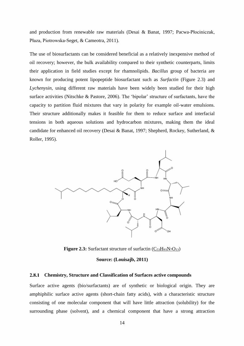
their application in field studies except for rhamnolipids. Bacillus group of bacteria are

known for producing potent lipopeptide biosurfactant such as Surfactin (Figure 2.3) and

Lychenysin, using different raw materials have been widely been studied for their high

surface activities (Nitschke & Pastore, 2006). The ‘bipolar’ structure of surfactants, have the

capacity to partition fluid mixtures that vary in polarity for example oil-water emulsions.

Their structure additionally makes it feasible for them to reduce surface and interfacial

tensions in both aqueous solutions and hydrocarbon mixtures, making them the ideal

candidate for enhanced oil recovery (Desai & Banat, 1997; Shepherd, Rockey, Sutherland, &

Roller, 1995).

Figure 2.3: Surfactant structure of surfactin (C53H93N7O13)

Source: (Louisajb, 2011)

Chemistry, Structure and Classification of Surfaces active compounds

Surface active agents (bio/surfactants) are of synthetic or biological origin. They are

amphiphilic surface active agents (short-chain fatty acids), with a characteristic structure

consisting of one molecular component that will have little attraction (solubility) for the

surrounding phase (solvent), and a chemical component that have a strong attraction

https://pubchem.ncbi.nlm.nih.gov/search/#collection=compounds&query_type=mf&query=C53H93N7O13&sort=mw&sort_dir=asc

15

(solubility) for the surrounding phase. In these aqueous system, the hydrophobic (their tails)

is the nonpolar chain hydrocarbon and hydrophilic (their heads) or polar end moieties that

reduce the surface tension of a liquid, the interfacial tension between two liquids, or that

between a liquid and a solid of the medium in which they are dissolved (Taylor, 2001). A

schematic of a surfactant molecule structure is shown in Figure 2.4.

Figure 2.4: Structure of a (bio/surfactant) molecule

Source: (Salehi, 2009)

de Guertechin, (2001) classified surfactants into four general groups, and it is the nature of

the polar head group which is important to apportion surfactants into various categories.

These groups are; anionic, (negative charge), cationic (positive charge), nonionic (wetting

agent), and zwitterionic (both a negative and a positive charge). These materials have the

tendency to adsorb at the interfaces of a system, or to form aggregates in solution at very low

molar concentrations.

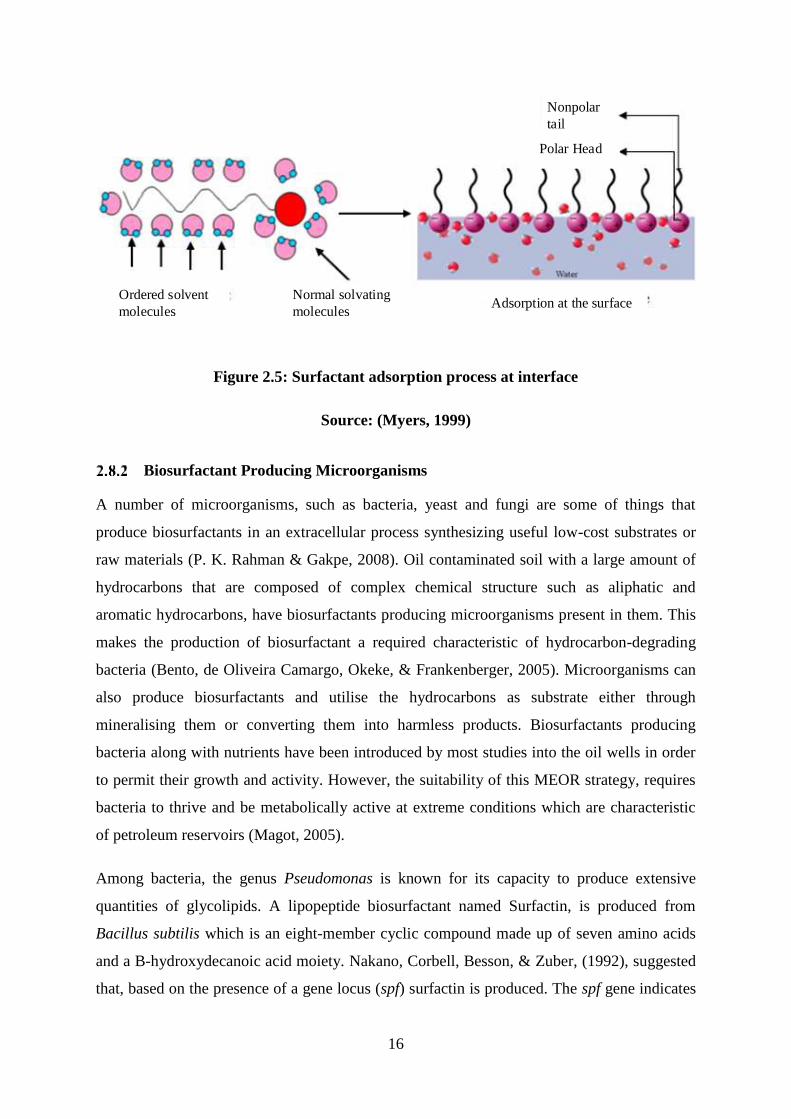
This surfactant adsorption phenomenon can be explained thus that when a surfactant is

dissolved in a solvent (water), the hydrophobic group causes an unfavourable distortion

(ordering) of the liquid structure and the result would be an increase in the overall free energy

of the system and a decrease in the overall entropy of the system as seen in Figure 2.5. This

entropy of the system can be regained when surfactant molecules are transferred to an

interface and the associated water molecules are released. Therefore, the surfactant will

adsorb, or it may undergo some other process like micelle formation to lower the energy of

the system. On the other hand, the presence of surfactant molecules at the interface decreases

the amount of work required to increase the interfacial area, resulting in a decrease of surface

or interfacial tensions.

16

Ordered solvent

molecules

Normal solvating

moleculesAdsorption at the surface

Nonpolar

tail

Polar Head

Figure 2.5: Surfactant adsorption process at interface

Source: (Myers, 1999)

Biosurfactant Producing Microorganisms

A number of microorganisms, such as bacteria, yeast and fungi are some of things that

produce biosurfactants in an extracellular process synthesizing useful low-cost substrates or

raw materials (P. K. Rahman & Gakpe, 2008). Oil contaminated soil with a large amount of

hydrocarbons that are composed of complex chemical structure such as aliphatic and

aromatic hydrocarbons, have biosurfactants producing microorganisms present in them. This

makes the production of biosurfactant a required characteristic of hydrocarbon-degrading

bacteria (Bento, de Oliveira Camargo, Okeke, & Frankenberger, 2005). Microorganisms can

also produce biosurfactants and utilise the hydrocarbons as substrate either through

mineralising them or converting them into harmless products. Biosurfactants producing

bacteria along with nutrients have been introduced by most studies into the oil wells in order

to permit their growth and activity. However, the suitability of this MEOR strategy, requires

bacteria to thrive and be metabolically active at extreme conditions which are characteristic

of petroleum reservoirs (Magot, 2005).

Among bacteria, the genus Pseudomonas is known for its capacity to produce extensive

quantities of glycolipids. A lipopeptide biosurfactant named Surfactin, is produced from

Bacillus subtilis which is an eight-member cyclic compound made up of seven amino acids

and a B-hydroxydecanoic acid moiety. Nakano, Corbell, Besson, & Zuber, (1992), suggested

that, based on the presence of a gene locus (spf) surfactin is produced. The spf gene indicates

17

production of biosurfactant in many Bacillus species creating the basis of the study conducted

by (Hsieh, Li, Lin, & Kao, 2004). Candida bombicola and Candida lipolytica are among the

most commonly studied yeast for the production of biosurfactants (Campos et al., 2013).

Most of the biosurfactants are known for their high molecular weight lipid complexes which

are normally produced under highly aerobic conditions. Ex-situ production in aerated

bioreactors makes this production achievable. The in-situ production (and action) becomes

advantageous when their large-scale application and soil is encountered. Maintenance of

anaerobic microorganisms and their anaerobic synthesis of biosurfactants are required when

there is low oxygen availability under the conditions outlined above. Therefore, screening for

anaerobic biosurfactants producers in these conditions is of immense importance (M. J.

McInerney, Javaheri, & Nagle, 1990).

Biosurfactant in the Petroleum Industry

The hypothesis for use of microorganisms in the improvement of oil recovery was initially

proposed for the first time by Beckman in 1926. Zobell was the first to carry out investigation

of petroleum microbiology with application in microbial enhanced oil recovery and this

provided a base for researchers to carry out further experiments in that area. The results of

these investigations have constantly revealed that under reservoir conditions such as high

temperature, pressure and salinity, certain microbes along with proper nutrients and bio-

catalysts can grow and produce biosurfactants, alcohols, bio-polymers, gases and acids as

metabolic by products (Zobell, 1946). By altering saturations and rock wettability these

metabolic products can displace trapped oil thus, resulting in enhanced oil recovery from oil

reservoirs.

According to Zobell the main mechanisms behind oil release from permeable media are

processes such as bacterial metabolites that break up inorganic carbonates; bacterial gases

which reduce the viscosity of oil, thus increasing its flow; surface-active substances or

wetting agents produced by some microbes; and the high affinity of bacteria for solids to

crowd off the oil films, processes by which bacterial products (gases, acids, solvents, surface-

active agents, and cell biomas) releasing oil from the sand pack columns in wet labs were

patented by Zobell (Shibulal et al., 2014).

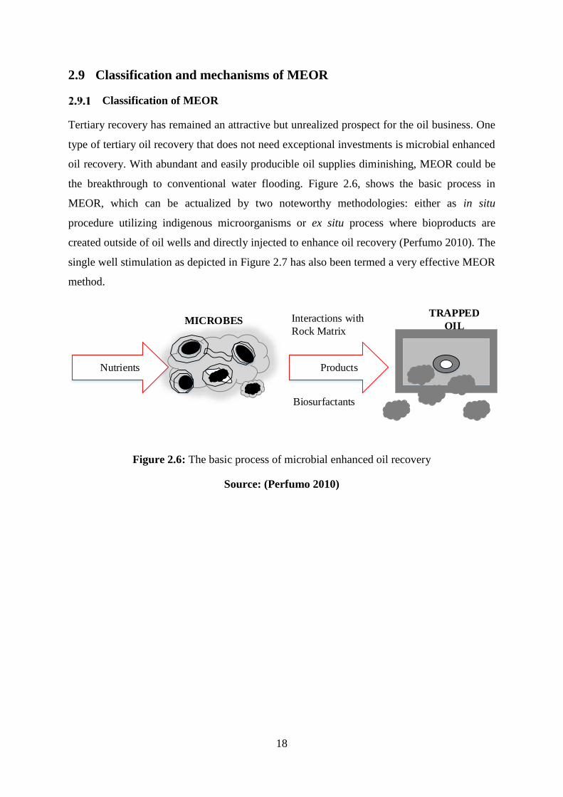
18

2.9 Classification and mechanisms of MEOR

Classification of MEOR

Tertiary recovery has remained an attractive but unrealized prospect for the oil business. One

type of tertiary oil recovery that does not need exceptional investments is microbial enhanced

oil recovery. With abundant and easily producible oil supplies diminishing, MEOR could be

the breakthrough to conventional water flooding. Figure 2.6, shows the basic process in

MEOR, which can be actualized by two noteworthy methodologies: either as in situ

procedure utilizing indigenous microorganisms or ex situ process where bioproducts are

created outside of oil wells and directly injected to enhance oil recovery (Perfumo 2010). The

single well stimulation as depicted in Figure 2.7 has also been termed a very effective MEOR

method.

Nutrients Products

Biosurfactants

Interactions with

Rock MatrixMICROBES

TRAPPED

OIL

Figure 2.6: The basic process of microbial enhanced oil recovery

Source: (Perfumo 2010)

19

Figure 2.7: Cyclic microbial oil recovery

Source: (Hsieh et al., 2004)

MEOR mechanism

The main mechanism for MEOR process is identified based on the end products generated

from bacteria metabolism. Rock dissolution, reduction in viscosity and permeability were

classified as some of the main mechanisms for MEOR (Janshekar 1985). These mechanisms

are similar to that of chemical EOR technique with a difference in the required products

coming from bacteria metabolism, and it’s expected to satisfy the basic law of

thermodynamics. These mechanisms have been proposed to take place through solubilisation,

mobilisation, or emulsification, increasing the contact area of hydrocarbons (Santos et al.,

2016), as shown in Figure 2.8. More so, it is very necessary to know the characteristics of a

reservoir before selection of the type of microbe to use since MEOR mechanism could differ

from bacteria to bacteria.

20

Production well

Oil

Injection

well

(Single 5-Spot Pattern Shown)

Injection

fluids

Injection

pump

Driving Fluid

(water)

Fresh Water

Buffer to Protect

biosurfactant

Biosurfactant

Solution for

Mobility Control

Micellar Fluid

for Releasing

Oil

AdditionalOil

Recovery (Oil

Bank)

Preflush to

Control

Reservoir

Figure 2.8: Microbial flooding recovery

Source: (Sheehy, 2008)

2.10 Influence of culture medium composition on biosurfactant production

The productions of biosurfactants are seen predominantly during their growth on water

immiscible substrates. However, biosurfactants may be produced by some yeast in the

presence of different forms of substrates, like carbohydrates. The usage of different carbon

sources changes the structure of biosurfactant produced and its properties, and can be

exploited to get products with preferred properties for specific applications.

Several investigations carried out relating to the optimization of the physicochemical

properties in biosurfactant production, have shown some similarities in the culture conditions,

in developing these microbes. In almost all cases, the inoculum used was prepared and

incubated overnight, which is the ideal procedure for better results. However, in some

experiments the inoculum was isolated from an oil contaminated soil. Based on literature

biosurfactants have been cultured at different ranges of temperature and pH in a controlled

fermenter. For example, Anita and Roberto, (2014) used vinasse as a substrate in the

fermentation process for the production of biosurfactants well as inoculum fermentation

media by Bacillus subtilis PC, in order to reduce environmental impacts generated by this

effluent and cut down production costs. The operating conditions; temperature and stirring

rate where kept constant at 30oC and 120 rpm, and pH value of 6.5. The successful isolation

21

of an anaerobic thermophilic bacterium named AR80 was evaluated by Purwasena, Sugai, &

Sasaki, (2014) to know its probability as a candidate for MEOR. It was identified as a strain

belonging to the Petrotoga sp. AR80 decreased the oil viscosity by 60% in the culture

medium and grew well in a reservoir of brine supplemented with yeast extract (0.05 g/l). The

most suitable conditions in which AR80 grows well are at temperatures between 50oC and

70oC and at salinity of <30 g/L. The core flooding experiment revealed that this bacterium

can possibly enhance MEOR and reduce excessive costs.

The production experiments of Bacillus subtilis lipopeptide biosurfactant was carried out at

37oC and at pH 7.0 (Ghribi and Ellouze, 2011), using carbohydrate as the carbon source and

ammonium chloride as inorganic nitrogen source. The inocula was incubated in a rotatory

shaker at 200rpm and kept overnight. Special conditions were devised to produce

biosurfactant from three Candida strains at culture conditions of temperature, 20oC and pH

7.0 (Mandy et al., 2012). Sucrose concentration of 1.0% and (NH4)2SO4 concentration of 12%

nitrogen source was best for biosurfactant production. Yields of biosurfactants grown on

Bacillus licheniformis strain were considerably higher in cultures grown anaerobically at a

C/N ratio of 1:24, pH 7.0, and temperature of 30oC. Concentrations of NaCl and Na2S and on

water characteristics in the medium broth favoured biosurfactant production (Gogotov and

Miroshnikov, 2009).

Carbon Source

Carbon is a very essential component of media for microbial growth and different

microorganisms that produce biosurfactant. It is therefore important to select a suitable

carbon supplements which would affect the composition of the produced biosurfactant. A

biosurfactant produced by Y. lipolytica IA 1055 was identified by Sarubbo et al., (2001),

using glucose as a carbon source and concluded that the stimulation of biosurfactant

production is independent on the presence of hydrocarbons. Kitamoto et al., (2001) studied

the production of mannosylerythritol lipids (MEL), a biosurfactant produced by Candida

antarctica, using different n-alkanes as carbon source. The productivity of MEL was

significantly affected by the chain-length of the alkane substrates, with the highest

productivity obtained from n-octadecane. Zinjarde & Pant, (2002), demonstrated the

surfactant biosynthesis by Y. lipolytica NCIM 3589 using soluble carbon source such as

glycerol, glucose and sodium acetate. Reduction is surface tension was better when glucose,

sucrose, yeast extract, beef extract, sodium pyruvate and tri sodium citrate were used as

22

carbon sources. Mannan-proteins have been produced by Kluyveromyces marxianus, using

lactose as the soluble substrate (Lukondeh, Ashbolt, & Rogers, 2003). The soy molasses, a

by-product from the production of soyabean oil, plus oleic acid were tested as carbon sources

for the production of sophorolipids by the yeast C. bombicola (Solaiman, Ashby, Nuñez, &

Foglia, 2004). Recently, Karimi, Mahmoodi, Niazi, Al-Wahaibi, & Ayatollahi, (2012)

investigated Enterobacter cloacae strain which produced different amounts of biosurfactants

in the growth culture, using sucrose and n-dodecane as the carbon source. Results indicated

that E. cloacae had the ability to adhere to the desired surface. The described carbon source,

like glycerol, glucose, acetates and other organic acids, as well as pure n-alkanes are quite

expensive and cannot reduce the cost of biosurfactant production. An approach to lessen the

cost is partial or complete replacement of pure reagents with industrial/agricultural mixtures

(Saharan, Sahu, & Sharma, 2012).

Nitrogen Source

Nitrogen is important in the biosurfactant production medium because it is an essential

component of the proteins that are essential for the growth of microbes and for production of

enzymes for the fermentation process. Several sources of nitrogen have been used for the

production of biosurfactants, such as sodium nitrate, meat extract and malt extract (Mata-

Sandoval, Karns, & Torrents, 2001), urea, peptone, ammonium sulphate, ammonium nitrate

(Thanomsub et al., 2004). Yeast extract is the most widely used nitrogen source for

biosurfactant production, but its required concentration depends on the nature of

microorganism and the culture medium to be used. The production of biosurfactants often

occurs when the nitrogen source is depleted in the culture medium, during the stationary

phase of cell growth. Lukondeh et al., (2003) investigated the production of biosurfactant by

K. marxianus FII 510700 using yeast extract (2 g L-1) and ammonium (5 g L-1) as nitrogen

sources.

The composition and characteristics of biosurfactants are influenced by the external electron

acceptor for respiration, nature of the nitrogen source, presence of sulphur, manganese, iron,

magnesium and phosphorus in the media. Therefore, the fundamental factors for

understanding, forecasting and designing MEOR projects successfully is to determine which

mechanisms that allow bacteria to increase oil recovery (Shabani Afrapoli, Nikooee, Alipour,

& Torsater, 2011).

23

2.11 Economical and promising alternatives for Biosurfactant Production

For the production of commercially viable biosurfactants, the development of efficient and

successfully optimized bioprocesses, including optimization of the culture conditions and

cost-effective recovery processes for maximum biosurfactant production and recovery needs

to be improved. More so, the use of inexpensive and waste substrate for the formulation of

fermentation media which lower the initial raw material costs involved in the process needs

to be harnessed. The use of agro-based low-cost raw materials (Table 2.1), have been

explored extensively and were found to be suitable for microbial growth and substrates for

biosurfactant production (Al-Bahry et al., 2013; Joshi et al., 2008).

2.12 Biosurfactants as potential candidate for wetting agents

In investigating wettability alteration at pore scale, Karimi et al., (2012) used Enterobacter

Cloacae strain which produced different amounts of biosurfactants in the growth culture,

using sucrose and n-dodecane as the carbon source. This strain which was isolated from an

oil contaminated soil sample is a facultive anaerobic gram-negative bacterium that changed

the wettability towards water-wet state. High amounts of biosurfactants were produced from

E. cloacae and when n-dodecane was used, it considerably reduced the surface tension. Also

the contact angle measurement high-lighted the importance of inclusion of microbial cells for

wettability alteration. (Afrapoli, Crescente, Alipour, & Torsaeter, 2009), revealed the

effectiveness of Rhodococcus sp. 094 (an alkane oxidizing bacteria), to increase oil

recoveries from Berea sandstone cores using the Amott index method. The bacteria was

isolated from the sea water (fjord of Trondheim) that has the tendency of extremely forming a

stable crude oil-in-water emulsion. Interfacial tension reduction and the effect of wettability

on residual oil saturation resulted during metabolic activities. The experimental results by

Kowalewski, Rueslåtten, Steen, Bødtker, & Torsæter, (2006), showed the importance of

bacterial on IFT reduction and wettability change towards water wet. The oil degrading

bacteria (Aerobic mesophilic) used, grew on the oil-water interface with saturated sandstone

core and cultured at temperatures between 20oC-45oC for optimum growth. However, the

core (sandstone) experiment carried out revealed a low total production of oil. It is interesting

to note here that the growing of bacteria in this interface can result to a major increase in oil

recovery upon water flooding. The application of bacterial/fungal biofilms on quartz resulted

in wettability changes in the direction of more oil wet, characterized by high dome-spherical

droplets of water, with contact angle of greater than 90oC (Polson et al., 2010).

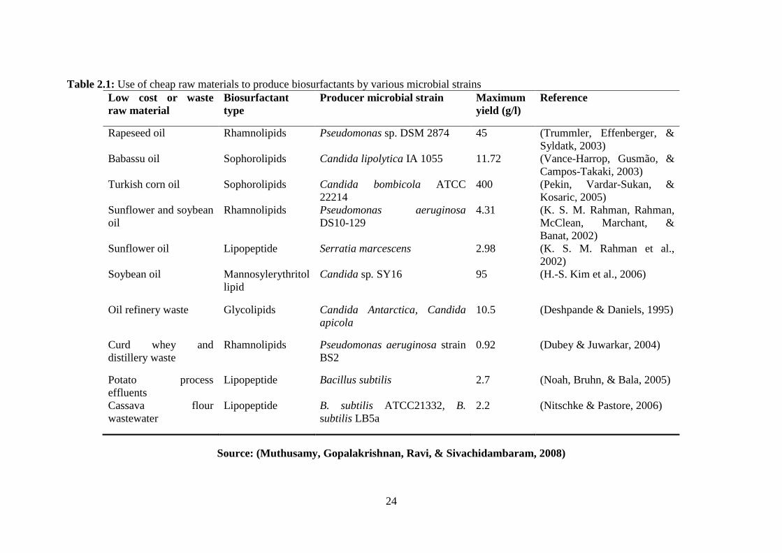
24

Table 2.1: Use of cheap raw materials to produce biosurfactants by various microbial strains

Low cost or waste

raw material

Biosurfactant

type

Producer microbial strain Maximum

yield (g/l)

Reference

Rapeseed oil Rhamnolipids Pseudomonas sp. DSM 2874 45 (Trummler, Effenberger, &

Syldatk, 2003)

Babassu oil Sophorolipids Candida lipolytica IA 1055 11.72 (Vance-Harrop, Gusmão, &

Campos-Takaki, 2003)

Turkish corn oil Sophorolipids Candida bombicola ATCC

22214

400 (Pekin, Vardar-Sukan, &

Kosaric, 2005)

Sunflower and soybean

oil

Rhamnolipids Pseudomonas aeruginosa

DS10-129

4.31 (K. S. M. Rahman, Rahman,

McClean, Marchant, &

Banat, 2002)

Sunflower oil Lipopeptide Serratia marcescens 2.98 (K. S. M. Rahman et al.,

2002)

Soybean oil Mannosylerythritol

lipid

Candida sp. SY16 95 (H.-S. Kim et al., 2006)

Oil refinery waste Glycolipids Candida Antarctica, Candida

apicola

10.5 (Deshpande & Daniels, 1995)

Curd whey and

distillery waste

Rhamnolipids Pseudomonas aeruginosa strain

BS2

0.92 (Dubey & Juwarkar, 2004)

Potato process

effluents

Lipopeptide Bacillus subtilis 2.7 (Noah, Bruhn, & Bala, 2005)

Cassava flour

wastewater

Lipopeptide B. subtilis ATCC21332, B.

subtilis LB5a

2.2 (Nitschke & Pastore, 2006)

Source: (Muthusamy, Gopalakrishnan, Ravi, & Sivachidambaram, 2008)

25

2.13 Waterflooding

A predominant fraction of the world’s oil reservoirs is produced by the solution gas drive

mechanism (Gulick & McCain Jr, 1998). This drive mechanism has low energy and thus

leaving behind large quantities of oil trapped in small pores of the rock formation, when the

production reaches its economic limit. In addition, poor displacement efficiency, viscosity

forces and reservoir heterogeneities contributes to the problem of leaving behind huge

reserves of unproduced oil (Elraies & Tan, 2012; D. K. F. Santos, Rufino, Luna, Santos, &

Sarubbo, 2016). One of the cheapest and most popular means of maintaining and restoring

reservoir energy is waterflooding. Waterflooding is the most predominant improved recovery

process in both onshore and offshore regions. This recovery method consists of injecting

water through an injector well to push oil to the producing wellbore, which can lead to an

increase of total recovery up to 40 – 50% of OOIP (Bachmann et al., 2014).

The history of waterflooding goes back to the 1860s. However, the use of waterflooding as a

means of recovery was not widely accepted until the 1950’s where there was discovery of

several gigantic reservoirs (i.e. Wasson, Slaughter, Levelland, North and South Cowden,

Means, and Seminole) in West Texas (Gulick & McCain Jr, 1998). These reservoirs were

found in highly heterogeneous shallow shelf carbonates and had a solution gas drive

mechanism. Thus, the reservoir energy depleted within a few years and producing rates

rapidly dropped. Consequently, it was crucial to find a way to restore and maintain the

reservoir energy, hence the wide use of water injection.

2.14 Biosurfactant flooding

MEOR is the tertiary recovery of oil in which microbes or their metabolic products are used

to enhance and recover residual oil. Zobell, (1946), patented a process for secondary oil

recovery, using anaerobic, hydrocarbon-utilising, and sulfate-reducing bacteria such as

Desulfovibrio species in situ. Updegraff & Wren, (1954), the proposed that this bacterium use

molasses as a nutrient to produce large amounts of organic acids and carbon dioxide to

enhance oil recovery in wet labs. In studies conducted by Bond, (1961), he injected 5,000 gal

of agar medium containing sand and Desulfovibrio hydrocarbonoclasticus into a sandstone

reservoir initially producing 15 bbl/day, at a depth of 3,000 ft. The well was shut for 3

months after injecting the inoculum, for the bacterial growth and action. After production

started again, the well produced 25 bbl/day.

26

The process of injecting bacterial spores along with nutrients into a reservoir was patented by

(ZoBell, 1947). In his findings, a medium containing molasses and spores of Clostridium

roseum was passed through a sand packed column saturated with oil. The spores would

germinate in the reservoir and enhance oil recovery from the reservoir rock, bringing about a

30% increase in oil recovery. Similar results in the release of oil was studied by A. Johnson,

(1979), inoculating a mixed culture of Bacillus and Clostridium spp. (1 to 10 gal) with crude

molasses and mineral salts as nutrients, in 150 stripper wells in the USA. These wells have an

average reservoir temperature of 38oC, depths 200 to 1000 ft, porosities were 10 to 30% and

producing at an average of 2 bbl/day. The additional recovery averaged between 20 to 30%

across all the wells. Yarbrough & Coty, (1983), reported increase in oil production from 0.6

bbl/day to 2.1 bbl/day in field test performed in Arkansas, after injecting Clostridium

acetobutylicum with a 2% solution of beet molasses, during aa 6-month period.

In the later works, Rebecca S Bryant & Douglas, (1988), utilised different bacterial strains in

Berea sandstone cores which gave additional recovery of 32% compared to water flooding,

and some spore forming bacteria even showed 50-60% additional oil recovery. A mixed

culture of aerobic and anaerobic bacteria with acid-hydrolysed substances from peat and soils

was introduced by (Kuznet︠s︡ov, 1963), and shut in the well for 6 months. When production

reopened, the rate of oil released rose to 300 bbl/day from 275 bbl/day. It is important to

know the right amount of bacterial to inject into the reservoir to prevent plugging of the pores

to allow for efficient mobilisation of microorganisms through the reservoir pore spaces. One

of the main function of biosurfactants is to reduce interfacial tension and in Section 3.3, the

IFT experiments were conducted and discussed in Section 4.3.

2.15 Theoretical Background of Pendant Drop Interfacial Tension

The drop shape analysis is a convenient way to measure interfacial tension with the following

two principal assumption; firstly, the drop is symmetric about a central vertical axis (it is

irrelevant from the direction the drop is viewed) and secondly, the drop is not in motion

implying that viscosity and inertia are playing a role in determining its shape (Woodward,

2013). The shape of a liquid drop being acted upon solely by gravitational and surface energy

forces is given by the Laplace equation,

𝛾 = ∆𝜌𝑔𝑅𝑂

2

𝛽 (2.10)

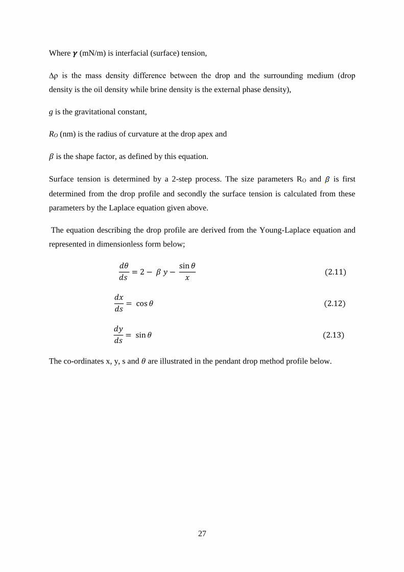
27

Where 𝜸 (mN/m) is interfacial (surface) tension,

∆ρ is the mass density difference between the drop and the surrounding medium (drop

density is the oil density while brine density is the external phase density),

g is the gravitational constant,

RO (nm) is the radius of curvature at the drop apex and

𝛽 is the shape factor, as defined by this equation.

Surface tension is determined by a 2-step process. The size parameters RO and is first

determined from the drop profile and secondly the surface tension is calculated from these

parameters by the Laplace equation given above.

The equation describing the drop profile are derived from the Young-Laplace equation and

represented in dimensionless form below;

𝑑𝜃

𝑑𝑠 = 2 − 𝛽 𝑦 −

sin 𝜃

𝑥 (2.11)

𝑑𝑥

𝑑𝑠= cos 𝜃 (2.12)

𝑑𝑦

𝑑𝑠= sin 𝜃 (2.13)

The co-ordinates x, y, s and 𝜃 are illustrated in the pendant drop method profile below.

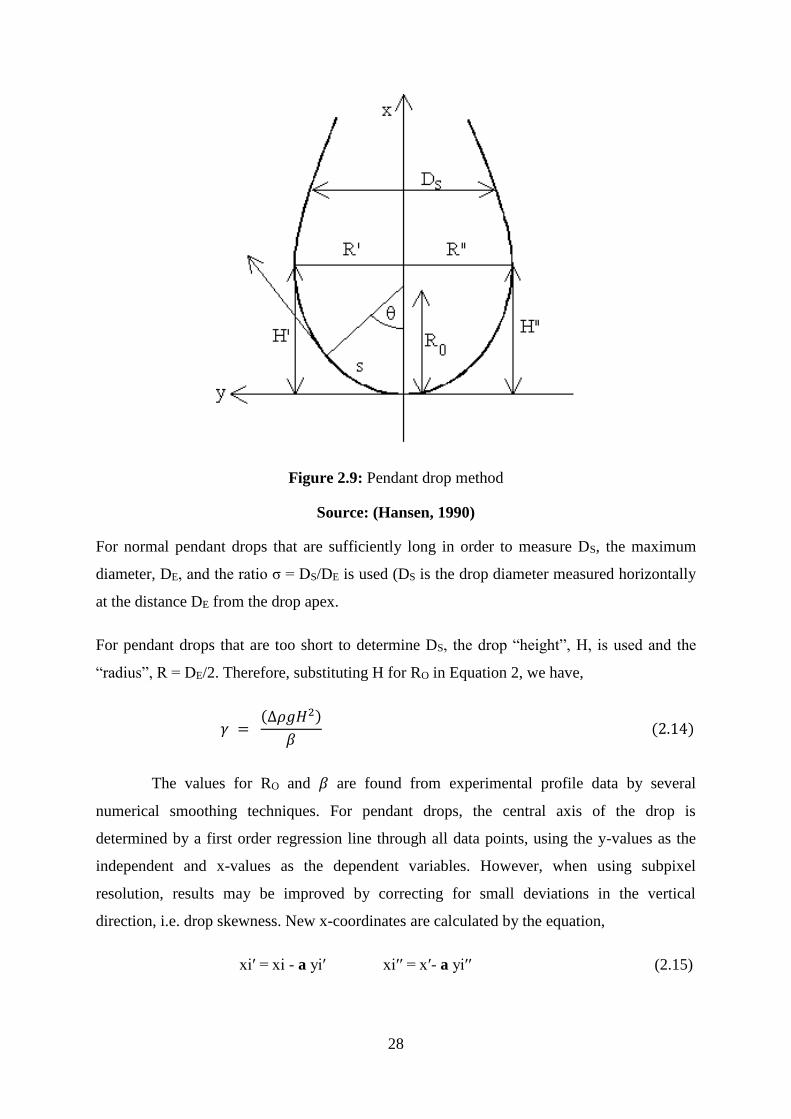
28

Figure 2.9: Pendant drop method

Source: (Hansen, 1990)

For normal pendant drops that are sufficiently long in order to measure DS, the maximum

diameter, DE, and the ratio σ = DS/DE is used (DS is the drop diameter measured horizontally

at the distance DE from the drop apex.

For pendant drops that are too short to determine DS, the drop “height”, H, is used and the

“radius”, R = DE/2. Therefore, substituting H for RO in Equation 2, we have,

𝛾 = (∆𝜌𝑔𝐻2)

𝛽 (2.14)

The values for RO and 𝛽 are found from experimental profile data by several

numerical smoothing techniques. For pendant drops, the central axis of the drop is

determined by a first order regression line through all data points, using the y-values as the

independent and x-values as the dependent variables. However, when using subpixel

resolution, results may be improved by correcting for small deviations in the vertical

direction, i.e. drop skewness. New x-coordinates are calculated by the equation,

xiʹ = xi - a yiʹ xiʹʹ = xʹ- a yiʹʹ (2.15)

29

Where xʹ and xʹʹ are the corrected coordinates for the left and right side of the drop,

respectively (yʹ and yʹʹ have opposite signs). More so, the y-values may be corrected in a

similar way by using the factor , but these corrections will be very small, because a

is very small, and may be neglected. For the determination of RO and 𝛽, the values for the

two sides are averaged; in addition, an asymmetry factor can be calculated from the equation,

Ass = (Hʹ – Hʹʹ)/ (Hʹ + Hʹʹ) (2.16)

Here, H is the drop “height”.

What needs to be considered when measuring surface and interfacial tension is the size of the

droplet used, which will help to achieve reliable results. At the point when measuring

interfacial tension, both density difference and interfacial tension have an impact on the

required droplet size. As a rule of thumb, smaller the density difference, bigger the droplet

has to be.

2.16 Measurement of Contact Angle

In measuring contact angle, this programme utilises a distinct technique which main strategy

uses the full theoretical drop profile that is ascertained in the curve fitting part of an

interfacial tension calculation. This implies that the entire drop must be visible, and that the

surface must be undisturbed, for example articles like rods and pipette should not be present.

Since every one of the conditions of interfacial tension must be satisfied, the contact angle

calculation will always be performed when interfacial tensions are measured. Of the

theoretical co-ordinates calculated by the numerical integration of the Young-Laplace

equation, not very many would coincide with the drop’s endpoint (the horizontal crosshair

cursor). The program will therefore interpolate between the two (2) points on each side of the

end, utilizing 2 extra points away in a cubic introduction method. This interpolation has been

shown to give exceptionally precise values compared to the exact theoretical calculation.

2.17 Chapter summary

This chapter began by explaining the significance of enhanced oil recovery,

influencing factors of remaining oil saturation, and an understanding of wettability. It

then detailed the use of biosurfactants in microbial enhanced oil recovery, and

identified the main mechanism for this process which includes; reduction in viscosity

permeability, rock dissolution, interfacial tension and wettability.

30

It further describes several culture medium for bacteria growth, which depend a lot on

the carbon source, as it can also change the structure of the biosurfactant produced.

This chapter also presented promising alternatives that are economical for

biosurfactant production, in-situ and ex situ biosurfactant flooding and a theoretical

understanding of the pedant drop equipment utilised later in this study.

The next chapter gives an illustration in a flow chart and discussion of the experimental

research methods that will help achieve this research objectives.

31

Chapter 3

3 Experimental Apparatus, Materials and Procedure

3.1 Overview

This Chapter describes the experimental procedures in Figure 3.1, which were utilised for the

successful progression of this study and details the steps involved to ensure that the results

obtained were accurate. This chapter covers four phases which includes:

Phase I – Microbial Culture: The isolation and reviving of selected microbes

from freeze dried condition was carried out in a fume cupboard to produce bio-

surfactants. A description of how the growth media is made is detailed in Section

3.2.1.4 As well as aseptically pouring of agar on petri dishes to prevent

contamination and further characterisation of these microbes to determine if they

are gram positive bacterial described in Section 3.2.2.1. Proper labelling of agar

plates and broths to include name (initials), date and code was ensured to prevent

any mix up and enable identification of the different species.

Phase II – Interfacial tension and Contact Angle: The assay used here for the

qualitative screening of the produced bio-surfactants was to check for possible

reduction in IFT/contact angle. An extensive experiment was carried out across

varying temperature, pressure and time to observe the different behaviours of the

bio-surfactants. A positive result could give an indication that the produced bio-

surfactants can possibly be utilised in enhancing oil recovery. The fluid sample

characteristics are detailed in Section 3.3.1.3 as well as the description of the

technique used is detailed in Section 3.3.1.1 using the DROPimage programme

designed by ramé-hart laboratory.

Phase III – Qualitative Wettability Tests: Two methods for qualitative

wettability tests is presented in summary which applies the principle of floatation

is described in Section 3.4. The rock grains will be treated with both the oil

sample and bio-surfactants to change the grain chemistry thus altering the

wettability. Two methods were implored which includes; the floating test and two-

phase separation test.

32

Phase IV - Coreflooding: A description of the core flooding experiment is

presented in Section 3.5.1.1 and consists of the major parts of the apparatus which

includes the injection system, core holder, the collection system and the data

acquisition and control system. The flooding was conducted using the BS-2

biosurfactant that gave the greatest reduction on interfacial tension of the crude

oil, to evaluate its treatment in effectively altering the wettability of Bandera Gray

sandstone to enhance oil recovery.

The flow chart (Figure 3.1) represents the steps of the experimental procedure in a summary.

33

Phase I

Microbial Culture

(Section 3.2)

Phase II

Interfacial Tension &

Contact Angle

(Section 3.3)

Phase III

Qualitative Wettability

Tests

(Section 3.4)

Phase IV

Core flooding

(Section 3.5)

Experimental

Apparatus and

Materials

(Section 3.2.1)

Errors &

Accuracy

(Section 3.3.3)

Errors &

Accuracy

(Section 3.4.3)

Errors &

Accuracy

(Section 3.2.3)

Procedure of data

collection

(Section 3.2.2)

Errors &

Accuracy

(Section 3.5.3)

Results & Discussion

(Chapter 4)

Experimental

Apparatus and

Materials

(Section 3.3.1)

Experimental

Apparatus and

Materials

(Section 3.4.1)

Experimental

Apparatus and

Materials

(Section 3.5.1)

Procedure of data

collection

(Section 3.3.2)

Procedure of data

collection

(Section 3.4.2)

Procedure of data

collection

(Section 3.5.2)

Figure 3.1: Structure and sequence of experimental methodology

34

3.2 Phase-1: Microbial Culture

Experimental Apparatus and Materials

3.2.1.1 Fume cupboard

The fume cupboard as seen in Figure 3.2, is a large piece of equipment, which was used in

the retrieval of the bacteria strains for biosafety, and to prevent contaminating the strains

from any external source. The principle of operation is simple: air is drawn in front (open)

side of the cabinet, and either expelled outside the building or made safe through filtration

and fed back into the room.

Figure 3.2: Retrieving of the selected bacteria strains

3.2.1.2 Eppendorf mastercycler® pro S

The PCR amplification was carried out with the Eppendorf Mastercycler pro S (Eppendorf

AG, Hamburg, Germany) which is a fast PCR cycler. It is used to control the temperature of

aqueous solutions, suspensions, and emulsions as seen in Figure 3.3. This equipment uses a

technique to amplify specific DNA fragments. Only a single DNA fragment is needed to

generate a million to a billion copies with a device like this. Tubes with the samples

consisting of the right ingredients are placed in the device to start the reaction, and a program

is set-up.

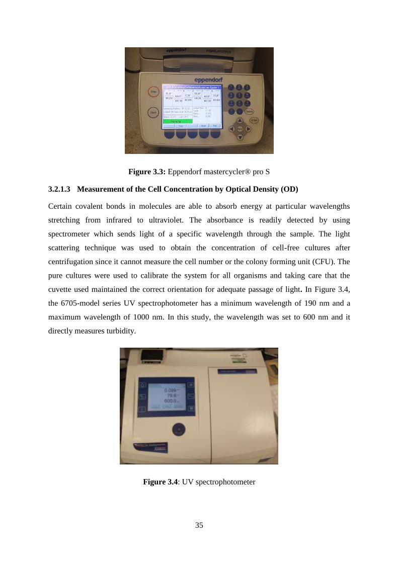
35

Figure 3.3: Eppendorf mastercycler® pro S

3.2.1.3 Measurement of the Cell Concentration by Optical Density (OD)

Certain covalent bonds in molecules are able to absorb energy at particular wavelengths

stretching from infrared to ultraviolet. The absorbance is readily detected by using

spectrometer which sends light of a specific wavelength through the sample. The light

scattering technique was used to obtain the concentration of cell-free cultures after

centrifugation since it cannot measure the cell number or the colony forming unit (CFU). The

pure cultures were used to calibrate the system for all organisms and taking care that the

cuvette used maintained the correct orientation for adequate passage of light. In Figure 3.4,

the 6705-model series UV spectrophotometer has a minimum wavelength of 190 nm and a

maximum wavelength of 1000 nm. In this study, the wavelength was set to 600 nm and it

directly measures turbidity.

Figure 3.4: UV spectrophotometer

36

3.2.1.4 Growth Media

Minimal salt medium: Sucrose (30 g L-1), KNO3 (5 g L-1), KH2PO4.2H2O (1 g L-1),

K2HPO4.2H2O (1 g L-1), NaCl (3 g L-1), MgSO4

.7H2O (0.2 g L-1), CaCl2H2O (0.2 g L-1), was

stirred in a duran with 1L distilled water for 30 minutes to mix thoroughly and pH was

adjusted to 6.8. The medium was then filter sterilzed using a 0.22µm filters and delivered into

ninety six (96) universal tubes to a volume of 10 mL each, using an electronic stripette as

seen in Figure 3.5. MSM medium was also filter sterilised into durans, containing 200ml and

400ml of media. These were to be the formation media for bacterial cultures, which the

interfacial measurements would be later carried out.

Figure 3.5: Liquid nutrient broths

3.2.1.5 Microorganism

As all oil reservoirs are essentially devoid of oxygen, anaerobic bacteria are generally

preferred in field applications. The types of bacteria used in this study are listed below and

are facultative anaerobes and are able to grow on nutrient agars (Table 3.1).

1. B. subtilis was obtained freeze dried from Leibniz Institute DSMZ-German Collection

of Microorganisms and Cell Cultures. The organism was maintained and stored as

recommended by DSMZ (Nakamura, Roberts, & Cohan, 1999).

2. B. licheniformis, type strain from Leibniz Institute DSMZ-German Collection of

Microorganisms and Cell Cultures (Chester, 1901), was maintained on nutrient agar at

37oC.

3. Paenibacillus polymyxa, type strain formally known as Bacillus polymyxa was

obtained from Leibniz Institute DSMZ-German Collection of Microorganisms and

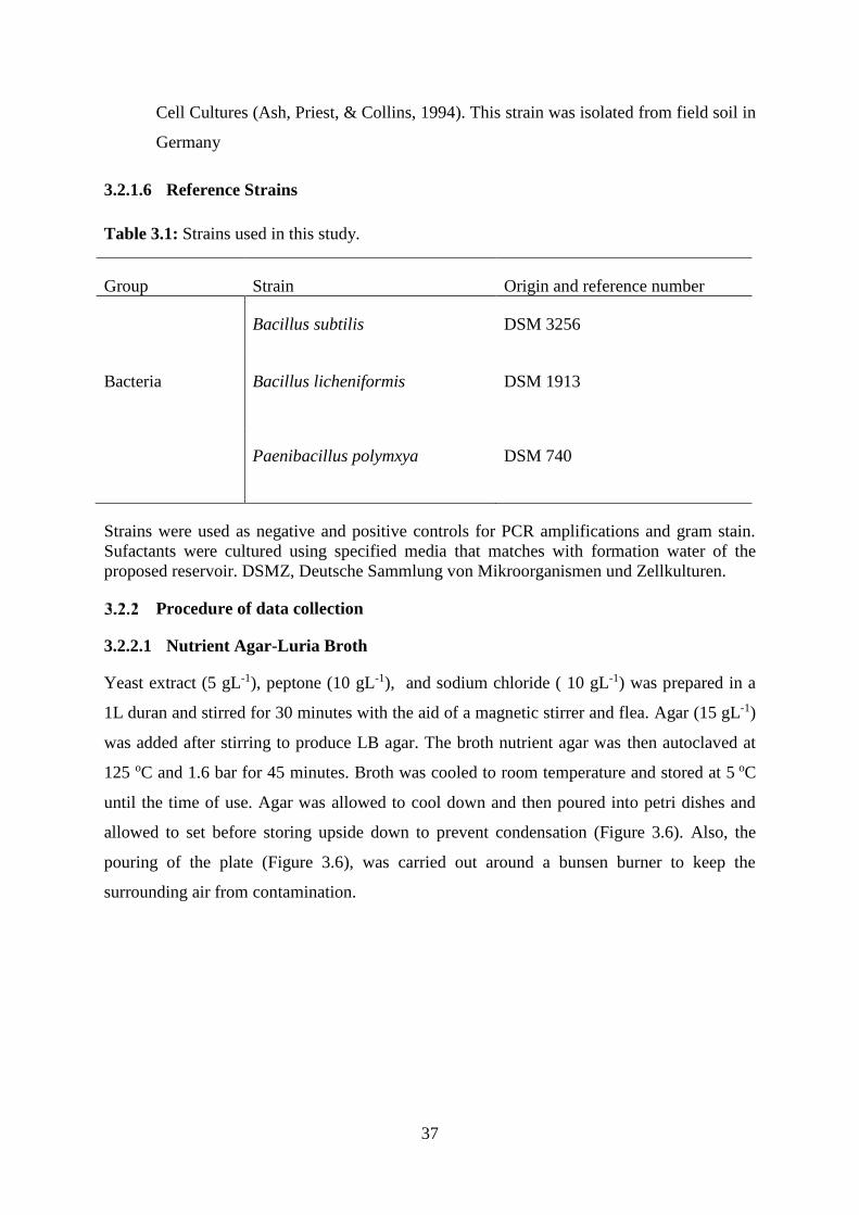
37

Cell Cultures (Ash, Priest, & Collins, 1994). This strain was isolated from field soil in

Germany

3.2.1.6 Reference Strains

Table 3.1: Strains used in this study.

Group Strain Origin and reference number

Bacillus subtilis

DSM 3256

Bacteria Bacillus licheniformis

DSM 1913

Paenibacillus polymxya

DSM 740

Strains were used as negative and positive controls for PCR amplifications and gram stain.

Sufactants were cultured using specified media that matches with formation water of the

proposed reservoir. DSMZ, Deutsche Sammlung von Mikroorganismen und Zellkulturen.

Procedure of data collection

3.2.2.1 Nutrient Agar-Luria Broth

Yeast extract (5 gL-1), peptone (10 gL-1), and sodium chloride ( 10 gL-1) was prepared in a

1L duran and stirred for 30 minutes with the aid of a magnetic stirrer and flea. Agar (15 gL-1)

was added after stirring to produce LB agar. The broth nutrient agar was then autoclaved at

125 oC and 1.6 bar for 45 minutes. Broth was cooled to room temperature and stored at 5 oC

until the time of use. Agar was allowed to cool down and then poured into petri dishes and

allowed to set before storing upside down to prevent condensation (Figure 3.6). Also, the

pouring of the plate (Figure 3.6), was carried out around a bunsen burner to keep the

surrounding air from contamination.

38

Figure 3.6: Pouring a plate of nutrient agar

3.2.2.2 Bacterial strain revival

This procedure was carried out in a fume cupboard, to prevent any external contamination.

Freeze dried strains (DSM 3256, DSM 1913 and DSM 740) were carefully removed from

glass tubes using a diamond cutter. 1000 µL of freshly prepared LB media was added to each

sample with the aid of generic filters to dissolve the freeze dried strains. The strains were left

for 20 minutes to dissolve properly and with the aid of a sterile innoculating loop it was

stirred to further aid dissolution.

3.2.2.3 Growth at Different Temperatures

The strains were plated on three (3) agar plates seperately and further innoculated into broths

previously made, imploring sterile innoculating loop and generic filters respectively. The

broth for the three samples where placed in a 30 oC shaking incubator to aid growing. Two

samples of the different strains on agar plates were placed in a 37 oC incubator and one

sample strain each in a 30 oC incubator to compare which temperature the bacteria grows

faster. The growth was checked periodically.

3.2.2.4 Stock Solution (Preservation of the Strains)

A stock solution is a concentrated solution that will be diluted to a lower concentration for

actual use. They help to conserve the strains and save preparation time. A stock solution was

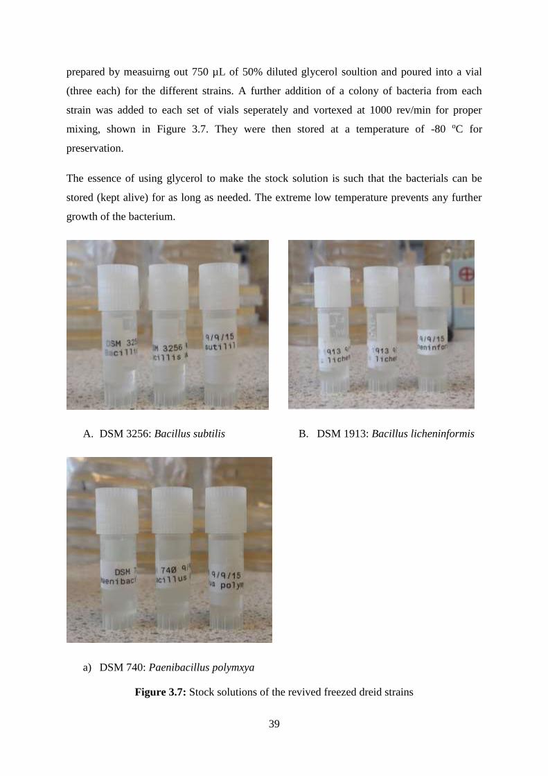
39

prepared by measuirng out 750 µL of 50% diluted glycerol soultion and poured into a vial

(three each) for the different strains. A further addition of a colony of bacteria from each

strain was added to each set of vials seperately and vortexed at 1000 rev/min for proper

mixing, shown in Figure 3.7. They were then stored at a temperature of -80 oC for

preservation.

The essence of using glycerol to make the stock solution is such that the bacterials can be

stored (kept alive) for as long as needed. The extreme low temperature prevents any further

growth of the bacterium.

A. DSM 3256: Bacillus subtilis B. DSM 1913: Bacillus licheninformis

a) DSM 740: Paenibacillus polymxya

Figure 3.7: Stock solutions of the revived freezed dreid strains

40

3.2.2.5 Determination of Phenotypic Characteristics

3.2.2.5.1 Colony Morphology of Microorganisms

On solid agar media, there are various physical appearance that colonies of bacterial and

fungal usually exhibit. Characteristics of colonies of a specific microbial species are

markedly stable. The characteristic morphology of a microbial colony ordinarily indicates

and likely proposes a particular type of microorganism upon examination of gross

morphology. Along these lines, any identification scheme for a microbial isolate ought to

begin with an intensive depiction of the appearances of colonies. Tentative identification of

type of organism (bacterial or fungal) and suspected genera or species, based on colonial

morphology, may help early avoidance of an extensive variety of other microbial types thus

reducing the number of potential candidates in the subsequent identification steps.

Furthermore, colonial morphology is critical in perceiving mutational changes in the

populace which occur upon repeated sub culturing of microbial strains. Mutant colonies

generally indicate changes in colonial properties, for example, surface, texture, or colour,

which can be easily separated from the wild sort. A description of colony characteristics more

often than not, includes the shape (structure), margin, elevation, optical properties, texture,

and pigmentation of the colonies.

3.2.2.5.2 Gram-Staining

The gram stain is the most important and universally used technique in the bacteriology

laboratory in differentiating bacterial species into two large groups (gram-positive and gram-

negative). This technique helps to understand how the gram stain reaction affects both

varieties of bacteria based on the biochemical and structural differences of their cell walls.

Gram-positives have a thick, moderately impermeable wall that resist decolorization and is

made out of peptidoglycan and secondary polymers. Gram-negatives has a thin peptidoglycan

layer in addition to an overlying lipid-protein bilayer known as the outer membrane, which

can be disturbed by decolorization (Beveridge, 2001).

The procedure is based on the ability of the microorganism to retain color of the stains used

during the stain reaction. Gram-positive bacteria are not decolorized by alcohol and will

remain as purple (retaining the initial violet stain). The gram-negative bacteria are

41

decolorized by the alcohol, losing the color of the primary stain, purple (hence show the pink

counter stain).

In the gram-stain method for each bacterium:

1. A loop full of the culture was spread on microscopic glass slides and first heat fixed

by passing the slide through flame for about 3 seconds until a thin film is formed and

allowed to dry.

2. The heat fixed smear was then stained with a basic dye, Crystal Violet, for 30

seconds, which is taken up in similar amounts by the bacteria.

3. After rinsing under tap water, the slides was treated with iodine (I2) for 30 seconds,

which is mordant to fix the stain.

4. The slides was then destained by washing briefly with acetone for 2 seconds.

5. Lastly, counterstained with a paler dye of different color (safranin) for 30 seconds. It

was then allowed to dry and viewed under a light microscope.

3.2.2.5.3 PCR Amplification

Polymerase Chain Reaction is an in vitro technique utilised in amplifying DNA sequences

with the aid of oligonucleotide primers that are complimentary to specific sequences in the

target gene (Willey, 2008; Wilson & Walker, 2010). The region of the chromosome for DNA

sequencing must be short comprising of variable sequence flanked by greatly conserved

region. To be able to differentiate microorganisms, their must be sufficient variability within

the selected sequence. Furthrmore the chosen sequence should not be horizontally

transmissible to other strains of species (Olive & Bean, 1999).

Subsamples of 3-10 ml of the media from the incubations were filtered through a 0.2 μm

filter in order to collect microbial cells on the filter surface. DNA extraction was carried out

using the method described by (Griffiths, Whiteley, O'Donnell, & Bailey, 2000) with

exception that 1 µg / µl-1 glycogen was added prior to the PEG precipitation stage to increase

nucleic acid precipitation efficiency. DNA quantification was performed using Qubit 3.0

Fluorometer and specified reagents (Life Technologies). Samples were stored at -20°C.

Bacteria 16S rRNA genes were amplified with polymerase chain reaction (PCR), using

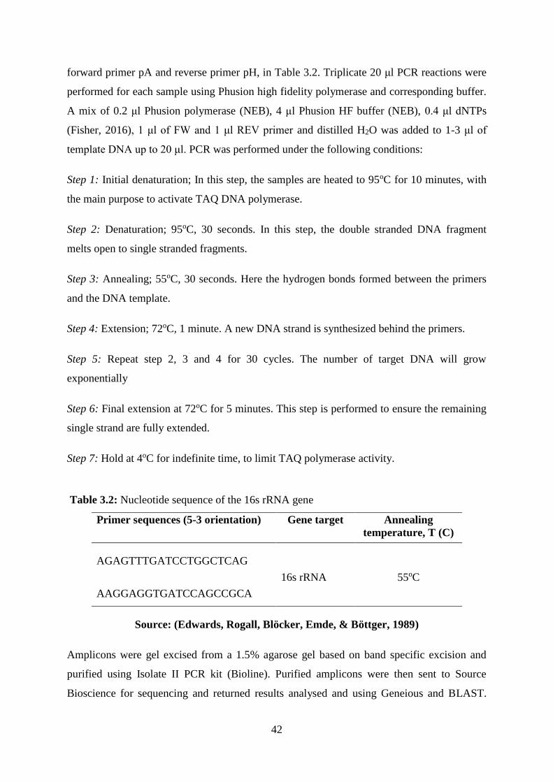
42

forward primer pA and reverse primer pH, in Table 3.2. Triplicate 20 μl PCR reactions were

performed for each sample using Phusion high fidelity polymerase and corresponding buffer.

A mix of 0.2 μl Phusion polymerase (NEB), 4 μl Phusion HF buffer (NEB), 0.4 μl dNTPs

(Fisher, 2016), 1 μl of FW and 1 μl REV primer and distilled H2O was added to 1-3 μl of

template DNA up to 20 μl. PCR was performed under the following conditions:

Step 1: Initial denaturation; In this step, the samples are heated to 95oC for 10 minutes, with

the main purpose to activate TAQ DNA polymerase.

Step 2: Denaturation; 95oC, 30 seconds. In this step, the double stranded DNA fragment

melts open to single stranded fragments.

Step 3: Annealing; 55oC, 30 seconds. Here the hydrogen bonds formed between the primers

and the DNA template.

Step 4: Extension; 72oC, 1 minute. A new DNA strand is synthesized behind the primers.

Step 5: Repeat step 2, 3 and 4 for 30 cycles. The number of target DNA will grow

exponentially

Step 6: Final extension at 72oC for 5 minutes. This step is performed to ensure the remaining

single strand are fully extended.

Step 7: Hold at 4oC for indefinite time, to limit TAQ polymerase activity.

Table 3.2: Nucleotide sequence of the 16s rRNA gene

Primer sequences (5-3 orientation) Gene target Annealing

temperature, T (C)

AGAGTTTGATCCTGGCTCAG

16s rRNA 55oC

AAGGAGGTGATCCAGCCGCA

Source: (Edwards, Rogall, Blöcker, Emde, & Böttger, 1989)

Amplicons were gel excised from a 1.5% agarose gel based on band specific excision and

purified using Isolate II PCR kit (Bioline). Purified amplicons were then sent to Source

Bioscience for sequencing and returned results analysed and using Geneious and BLAST.

43

The blast program (basic local alignment search tool) is a web search tool to show the

identity and similarity (99% - 99.5%) between different species belonging to the same genus.

3.2.2.6 Serial Dilution for bacterial strain

A set of serial dilutions was made for all three strains. In Figure 3.8, a sample of culture in a

broth was diluted to 10-7. Streak plating was then carried out using diluted solutions at 10-1,

10-4, and 10-6 on agar plates. This was done because agar plate allows accurate counting of

the microorganisms, resulting from the equal distribution across the plate. This cannot be

done with a fluid solution (broth).

In this study, the dilution series was calculated in the format below;

Figure 3.8: Serial dilution for bacteria strain

𝐷𝑖𝑙𝑢𝑡𝑖𝑜𝑛 𝑓𝑎𝑐𝑡𝑜𝑟 𝑓𝑜𝑟 𝑡𝑢𝑏𝑒 = 𝑎𝑚𝑜𝑢𝑛𝑡 𝑜𝑓 𝑠𝑎𝑚𝑝𝑙𝑒

𝑉𝑜𝑙𝑢𝑚𝑒 𝑜𝑓 𝑠𝑝𝑒𝑐𝑖𝑚𝑒𝑛 𝑡𝑟𝑎𝑛𝑠𝑓𝑒𝑟𝑒𝑑 +𝑣𝑜𝑙𝑢𝑚𝑒 𝑜𝑓 𝑑𝑖𝑙𝑢𝑒𝑛𝑡 𝑡𝑢𝑏𝑒 (3.1)

The total dilution factor = previous dilution factor of tube × dilution of the next tube

For this serial dilution;

1 ml culture = 10-1 for the first tube

0.1 ml added to 0.9 ml = previous dilution 10-1 (first tube) × 10-1 (second tube) = 10-2 total

dilution.

44

After successfully culturing, growing and testing the produced bio-surfactants in this section,

these bio-surfactants were then introduced into the formation water in a glass bottle at a ratio

of 1:1, with a total volume of 400 ml.

3.2.2.7 Biosurfactant Extraction Process

The biosurfactant was finally extracted and produced using the following protocol. A 400 ml

of prepared LB broth was inoculated at time point 0 to 0.1 Abs at 600 nm with the selected

bacterial culture. After 24-hour growth, cell-free supernatant from the culture broth was

obtained by centrifugation at 10,000 x g (m/s2) for 20 min at 4°C. The remaining cells were

removed by filtration using a 0.2 µM filters. The cell-free supernatant underwent acid

precipitation by adjusting the pH2 using 6 M HCl, and placed at 4°C overnight. The

precipitate was separated by centrifugation at a relative centrifugal force (RCF) of 10,000 x g

(m/s2) for 25 min at 4°C and extracted two times with methanol and solvent evaporated using

a rotary evaporator at 50°C (Pathak, Keharia, Gupta, Thakur, & Balaram, 2012). Finally, the

crude biosurfactant was collected and weighed for total surfactant extraction concentration.

Error and Accuracy

i. Sample specimen containers (petri dishes, test tubes) were correctly labelled to

include, name of the strain, date of preparation and initials of the collector.

ii. Safety precautions were put in place to avoid contamination of the samples, by

wearing safety gloves, and maintaining a sterile environment by flame sterilisation,

prior to processing the samples.

iii. The incubation temperature for growing the cultures was maintained for effective

growth rates.

iv. In using the UV spectrophotometer for measuring the absorbent, the system was first

calibrated at a wavelength of 600 nm, by firstly inserting the blank UV quartz

cuvettes which is the prepared media (substrate), and then followed with the bacteria

samples. This gave a tolerance of ±0.099.

3.3 Phase-II: Interfacial Tension and Contact Angle

As all oil reservoirs are essentially devoid of oxygen, anaerobic bacteria are generally

preferred in field applications. The types of bacteria used in this study are aerobic

microorganism. Bacillus are aerobic or facultative anaerobic (having the ability to be aerobic

45

or anaerobic) depending on the species. They are also facultative fermentative and can grow

on nutrient agar.

An extensive laboratory study was conducted for the measurement of the interfacial tension

between oil-synthetic formation water-bio-surfactant, covering pressure ranges of 0.15 to

13.89 MPa and temperatures of 26 to 75oC. The laboratory experiments were conducted

using the pendant drop method combined with the solution of the Laplace equation for

capillarity for the profile of the oil drop in the oil-brine equilibrium environment.

Measurements were made for each set of temperature and water salinity for pressures of

(0.15, 3.10, 5.10, 10.44, 12.51 and 13.89) MPa for a total of 285 IFT (mN/m) measurements.


3.3.1.1 The TEMCO Pendant Drop

Investigations of surface and interfacial tension by a pendant drop apparatus consists

typically of three parts: a viewing environmental chamber, temperature and pressure control,

and observation system to visualise the drop and a data acquisition system to infer the

interfacial tension from the pendant drop profile. This can be seen in the schematic sketch in

Figure 3.9 and complete set-up as seen in Figure 3.10. The IFT-10 Cell operates to 68.95

MPa (10000 psi) at 176 oC (350oF). Within this range, most reservoir conditions can be safely

simulated. The TEMCO Pendant Drop visual cell requires a light source to illuminate an oil

drop in its glass windowed chamber approximately 41.5 cm3 by volume. This pendant drop

method requires the fluid filling the cell to be transparent, to enable viewing of the drop of

the other fluid inside. In this study, with the aid of the pump, the brine-bio-surfactant flowed

from the continuous phase into the IFT cell (reservoir), while the oil sample flowed from the

drop phase through the capillary needle into the cell. The pendant oil drop (a clinging bubble

of oil in brine) was observed in silhouette by the low-power video microscope as seen in

Figure 3.11. In Figure 3.12, the temperature and pressure meter were used to regulate the

different variations of the reservoir conditions investigated and in turn, operating the

DROPimage Advanced software through the computer. The oil drop is equilibrated with

other fluids, and if desired, in contact with rock crystals, to simulate in-situ reservoir

conditions. Measurement of the oil drop dimensions and fluid densities enables calculation of

surface tension. Rigid film formation and aging effects may also be observed.

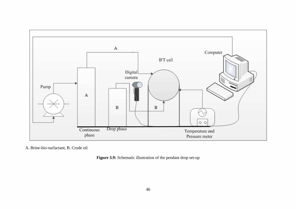
46

A. Brine-bio-surfactant, B. Crude oil

Figure 3.9: Schematic illustration of the pendant drop set-up

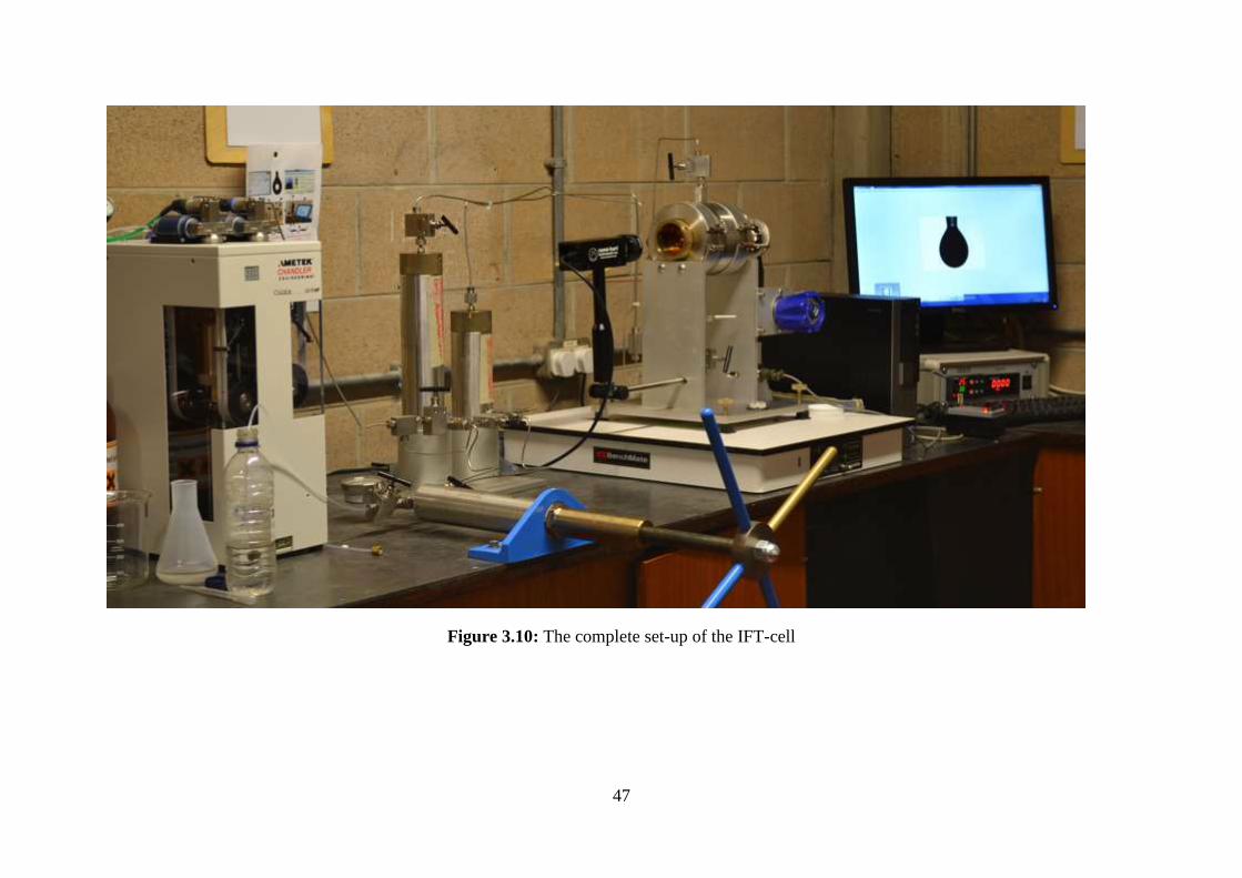
47

Figure 3.10: The complete set-up of the IFT-cell

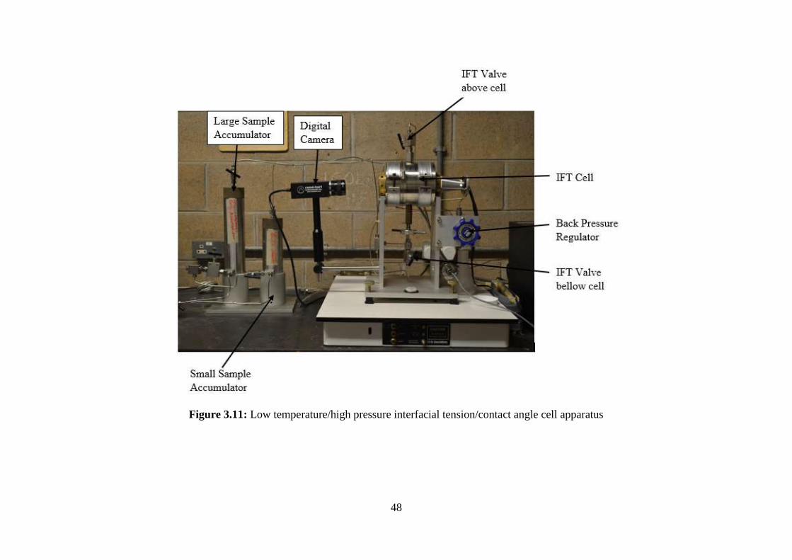
48

Figure 3.11: Low temperature/high pressure interfacial tension/contact angle cell apparatus

49

Figure 3.12: Pressure transducer/acquisition section

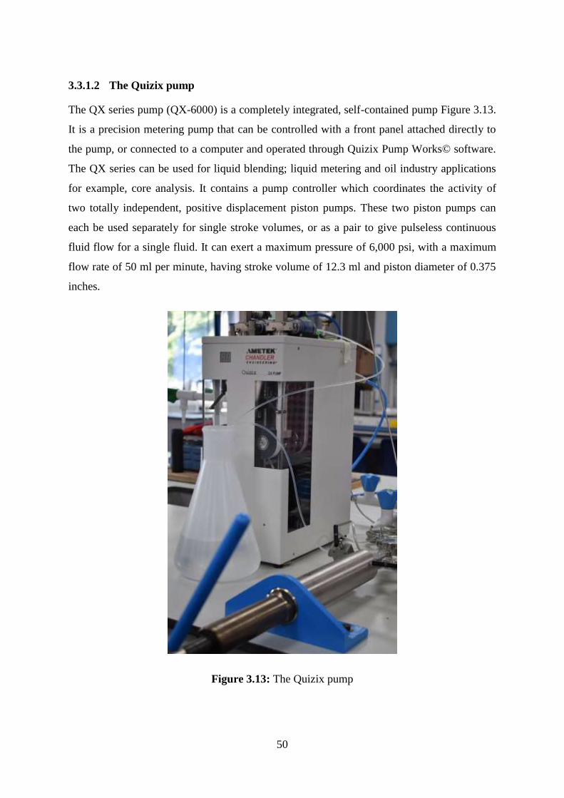
50

3.3.1.2 The Quizix pump

The QX series pump (QX-6000) is a completely integrated, self-contained pump Figure 3.13.

It is a precision metering pump that can be controlled with a front panel attached directly to

the pump, or connected to a computer and operated through Quizix Pump Works© software.

The QX series can be used for liquid blending; liquid metering and oil industry applications

for example, core analysis. It contains a pump controller which coordinates the activity of

two totally independent, positive displacement piston pumps. These two piston pumps can

each be used separately for single stroke volumes, or as a pair to give pulseless continuous

fluid flow for a single fluid. It can exert a maximum pressure of 6,000 psi, with a maximum

flow rate of 50 ml per minute, having stroke volume of 12.3 ml and piston diameter of 0.375

inches.

Figure 3.13: The Quizix pump

51

3.3.1.3 Fluid Samples

The characteristics of the crude oil from the Niger Delta oil field, and the composition of the

synthetic formation water are listed in Table 3.3 and Table 3.4 respectively, and shown in

Figure 3.14. The formation water used in this study was reconstructed in the laboratory on the

basis of specific formation water analysis from the formation of interest.

Table 3.3: Crude-oil Characteristics

API gravity Viscosity (cSt) Density (g/cm3) Salt Content

(ptb)

Classification

20.3 134.828 0.9322 13.9 Heavy oil

Figure 3.14: Crude oil and synthetic formation water

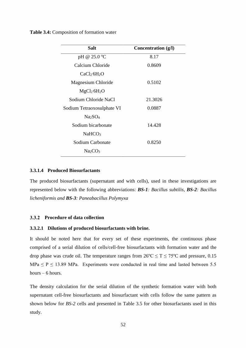
52

Table 3.4: Composition of formation water

Salt Concentration (g/l)

pH @ 25.0 oC 8.17

Calcium Chloride

CaCl2.6H2O

0.8609

Magnesium Chloride

MgCl2.6H2O

0.5102

Sodium Chloride NaCl 21.3026

Sodium Tetraoxosulphate VI

Na2SO4

0.0887

Sodium bicarbonate

NaHCO3

14.428

Sodium Carbonate

Na2CO3

0.8250

3.3.1.4 Produced Biosurfactants

The produced biosurfactants (supernatant and with cells), used in these investigations are

represented below with the following abbreviations: BS-1: Bacillus subtilis, BS-2: Bacillus

licheniformis and BS-3: Paneabacillus Polymyxa


3.3.2.1 Dilutions of produced biosurfactants with brine.

It should be noted here that for every set of these experiments, the continuous phase

comprised of a serial dilution of cells/cell-free biosurfactants with formation water and the

drop phase was crude oil. The temperature ranges from 26oC ≤ T ≤ 75oC and pressure, 0.15

MPa ≤ P ≤ 13.89 MPa. Experiments were conducted in real time and lasted between 5.5

hours – 6 hours.

The density calculation for the serial dilution of the synthetic formation water with both

supernatant cell-free biosurfactants and biosurfactant with cells follow the same pattern as

shown below for BS-2 cells and presented in Table 3.5 for other biosurfactants used in this

study.

53

Volume, V of solution = 100 ml

Weight of measuring cylinder (𝑊𝑡𝑐) = 47.12 g

𝑊𝑡𝑐 + formation water (𝐻2𝑂𝑓) = 146.45

𝑀𝑎𝑠𝑠, 𝑀 𝑜𝑓 𝐻2𝑂𝑓 = 𝑊𝑡𝑐 – (𝑊𝑡𝑐 + 𝐻2𝑂𝑓) (3.2)

𝑀 = 146.45 − 47.12 = 99.33

𝐷𝑒𝑛𝑠𝑖𝑡𝑦, 𝜌 = 𝑀

𝑉 (3.3)

𝜌 =99.33

100 = 0.9933 𝑔/𝑚3

Table 3.5: Density measurements for cultured biosurfactants

Biosurfactants Densities

BS-1 Cells 0.9863

BS-1 Cell-free 0.9763

BS-2 Cells 0.9933

BS-2 Cell-free 0.9823

BS-3 Cells 0.9939

BS-3 cell-free 0.9870

The volume of the produced biosurfactants were kept constant at 200 ml, for both cultures of

cells and cell-free. The biosurfactants where diluted serially with the synthetic brine to a ratio

of 1:1, thus the addition of 200 ml of synthetic brine with the aid of sterilised filters to

prevent contamination of the solution making the total solution 400 ml (Figure 3.15). For

optimum measurements, the calibration of the capillary tube was necessary before beginning

any experiment. The diameter of the needle was 3.03 mm and measured with the aid of a

digital Vernier calliper.

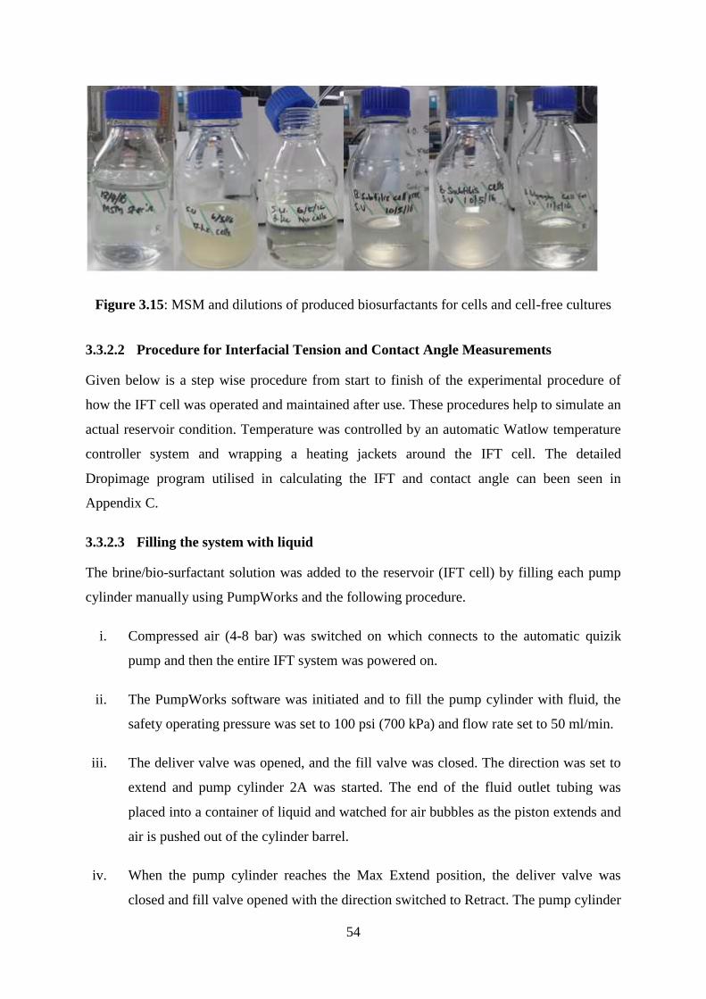
54

Figure 3.15: MSM and dilutions of produced biosurfactants for cells and cell-free cultures

3.3.2.2 Procedure for Interfacial Tension and Contact Angle Measurements

Given below is a step wise procedure from start to finish of the experimental procedure of

how the IFT cell was operated and maintained after use. These procedures help to simulate an

actual reservoir condition. Temperature was controlled by an automatic Watlow temperature

controller system and wrapping a heating jackets around the IFT cell. The detailed

Dropimage program utilised in calculating the IFT and contact angle can been seen in

Appendix C.

3.3.2.3 Filling the system with liquid

The brine/bio-surfactant solution was added to the reservoir (IFT cell) by filling each pump

cylinder manually using PumpWorks and the following procedure.

i. Compressed air (4-8 bar) was switched on which connects to the automatic quizik

pump and then the entire IFT system was powered on.

ii. The PumpWorks software was initiated and to fill the pump cylinder with fluid, the

safety operating pressure was set to 100 psi (700 kPa) and flow rate set to 50 ml/min.

iii. The deliver valve was opened, and the fill valve was closed. The direction was set to

extend and pump cylinder 2A was started. The end of the fluid outlet tubing was

placed into a container of liquid and watched for air bubbles as the piston extends and

air is pushed out of the cylinder barrel.

iv. When the pump cylinder reaches the Max Extend position, the deliver valve was

closed and fill valve opened with the direction switched to Retract. The pump cylinder

55

was re-started and as the piston retracts, fluid was drawn into the cylinder barrel. Then

on the next extend stroke mostly air was still delivered out of the fluid outlet fitting.

v. The procedure was repeated until a piston stroke was reached where no air bubbles

come out, only liquid. End with a retract stroke.

vi. After completely purging of air, the filling of the cell commenced. The automatic

pump valve 1B sample valve was connected to a 400 ml beaker already filled with

brine solution.

vii. The valve connecting the automatic pump to the outer phase (100cc accumulator) was

fully opened (counter-clock wise). Valve above outer phase accumulator was open

and valve below was closed. Valve above cell connected to contact angle was opened

and valve under cell connected to needle was closed. The Back Pressure (BP)

regulator was turned fully counter clockwise.

viii. The fill valve was opened to retract fluid in the piston, and deliver valve opened to

extend fluid into the continuous phase.

ix. This procedure continued until the cell (reservoir) was completely filled with brine

solution. And this was observed with fluid outing from the exit valve into a beaker.

x. The pump was then isolated by closing the valve that connects the pump and the

continuous phase accumulator and then switched off from the power source.

3.3.2.4 Pressurizing the IFT cell using the hand pump

i. The 400 ml beaker was filled with brine solution and connected to the manual pump

sample valve. The top and bottom valve connecting the 100cc and 50cc accumulator

was closed and the sample valve opened. The vacuum barrel of the hand pump was

filled with fluid on full counter-clock wise turning, close valve.

ii. Close valve above cell, connected to contact angle.

iii. To develop pressure, both valves connecting the outer phase and sample phase were

opened. The hand pump turned slowly in clockwise direction.

iv. When the required pressure was reached, the valve at the bottom of the outer phase

accumulator was closed. This was responsible for stabilizing the cell pressure.

56

v. The sample phase accumulator cover was opened and then oil sample was manually

poured into it until inside trend mark for its maximum filling is reached. Close cover.

vi. A continuous turning of the pump persisted to increase the gauge pressure to be above

the reservoir pressure. This was done in order to develop the pressure that will be

responsible for existence in the absence of air for release the drop into the cell.

vii. The valve below the IFT cell was slowly opened with fine adjustment to control the

sample drop.

viii. To de-pressurize the cell, the heater was first turned off and the cell was allowed to

gradually cool off. At room temperature, the remaining pressure was released slowly.

3.3.2.5 Experimental run/IFT measurement

i. Droping.exe file on the desktop was initiated, which opened a new experiment wizard

option box. Surface Tension-Pendant was selected.

ii. On clicking next, an option box to name the new experiment was displayed, and

SVU_IFT was entered.

iii. The drop phase was oil and formation water mixed with bio-surfactant was selected as

the outer phase. The solid phase was steel, which refers to the tip of the needle.

iv. This followed by setting the data for the experiment’s timing. Number of experiment

was selected to ten (10), and time interval of two (3) seconds. The wizard then saved

the choices in new parameter and method files.

v. The yes button was then clicked to start the experiment. The measure parameter box

appeared with the crosshair lines (vertical and horizontal).

vi. The drop was released to the near buoyant point. A picture of the drop was taken

using the camera button on the tool bar. Then the crosshairs were positioned correctly

on the drop for accurate readings, and the measure button was clicked to take

measurements. The IFT values were recorded.

vii. Before the readings were taken, the video setup was selected from the view option

box on the main window to adjust the video properties. This was necessary for clearer

viewing of the drop profile. The camera zoom was adjusted to 100%

57

3.3.2.6 Cleaning of the IFT Cell

A very important procedure in achieving reliable results for interfacial tension and contact

angle is a thorough cleaning of the apparatus, since contamination of trace amounts can alter

the measurement results.

i. Repetition of steps 1-10 in phase 1 with Hexane as the outer phase and sample phase

in order to flush out oil contaminants from the system.

ii. The valve under the IFT cell was unscrewed using spanner (size 19) which allowed

the draining of Hexane. The screwing of the valve followed immediately.

iii. Repetition of step 1 and 2 of phase 4 were carried out with Acetone as the outer phase

and sample phase to flush out Hexane.

iv. Repetition of steps 1-3 of phase 4 were carried out with distilled water as the outer

phase and sample phase to flush out the Acetone.

v. Repetitions of step 4 phase 4 with distilled water and heating the cell to at least a

temperature of 100oC for 15 mins. Temperature adjustment was achieved using the up

and down arrow buttons in the Watlow temperature controller to set the needed

temperature.

vi. The system was allowed to cool down to room temperature, before repeating step 2 of

phase 4 to expel the distilled water from the cell.

3.3.2.7 Precautions

Precautions must be observed since the IFT cell is a high-pressure/temperature system of

which some will aid in having accurate results:

Avoid close viewing of a high-pressure cell without protective eyewear in case of

a sudden glass window failure.

It is also advisable to place shields at each end of the window axis, especially if

the cell is left unattended.

Do not view the cell directly in line with the window: use the video system to

view the cell indirectly, or use a mirror to view the cell at an angle.

Avoid contact with exterior surfaces of the IFT Cell as it can become very hot.

58

It is necessary to always change the associated fluid densities in the software. This

will insure an accurate calculation.

Cell should be cleaned periodically to remove any heavy fluid build-up.

Error and Accuracy

i. For every IFT and contact angle measured, the oil film was assumed to be at

equilibrium 5 minutes after film formation, before then taking the measurements.

ii. For every single variable that was considered, the error given were calculated by the

program and given by the standard deviation between 0.02 to 0.12, of the regression

in the x-direction at the critical surface tension.

iii. Calibration of the total magnification in the system was always carried whenever

there was a change in optical magnification. Calibration was performed by measuring

the diameter of the needle (capillary tube), which is the solid phase.

iv. The time in which the mechanical equilibrium of the drop is reached, was highly

considered before commencing any measurement. With the help of a vibration-proof

table, this was achieved.

59

3.4 Phase-III: Qualitative Wettability Test

Qualitative wettability test will be performed on crushed rock material to check the

effectiveness of the core cleaning and aging procedures as well as the effectiveness of the

bio-surfactants in changing the wettability of the crude-oil aged crushed rocks.


3.4.1.1 The Soxhlet Extraction

It is important that the core be cleaned to a repeatable initial state (water-wet) that existed

before oil accumulated the formation. This process follows a procedure as discussed in

Section 3.4.3.1. The following are the apparatus used for the Soxhlet extraction process:

soxhlet extractor tube, glass thimble, reflux condenser tube (Figure 3.16), hose for water inlet

and outlet, extraction solvent – toluene, heating mantle, 500 ml round-bottom distillation

flask, retort stand (Figure 3.17), and fume cupboard. The heating mantle (temperature)

controller in Figure 3.18, is a single circuit, 10A 2400 Watts, 240V, that is used to manually

regulate the heating mantle with an adjustable output range from 5% to 100% of the rated

voltage.

Figure 3.16: Soxhlet kit

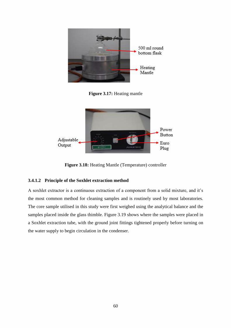
60

Figure 3.17: Heating mantle

Figure 3.18: Heating Mantle (Temperature) controller

3.4.1.2 Principle of the Soxhlet extraction method

A soxhlet extractor is a continuous extraction of a component from a solid mixture, and it’s

the most common method for cleaning samples and is routinely used by most laboratories.

The core sample utilised in this study were first weighed using the analytical balance and the

samples placed inside the glass thimble. Figure 3.19 shows where the samples were placed in

a Soxhlet extraction tube, with the ground joint fittings tightened properly before turning on

the water supply to begin circulation in the condenser.

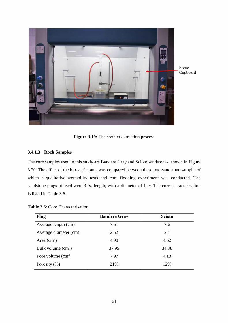
61

Figure 3.19: The soxhlet extraction process

3.4.1.3 Rock Samples

The core samples used in this study are Bandera Gray and Scioto sandstones, shown in Figure

3.20. The effect of the bio-surfactants was compared between these two-sandstone sample, of

which a qualitative wettability tests and core flooding experiment was conducted. The

sandstone plugs utilised were 3 in. length, with a diameter of 1 in. The core characterization

is listed in Table 3.6.

Table 3.6: Core Characterisation

Plug Bandera Gray Scioto

Average length (cm) 7.61 7.6

Average diameter (cm) 2.52 2.4

Area (cm2) 4.98 4.52

Bulk volume (cm3) 37.95 34.38

Pore volume (cm3) 7.97 4.13

Porosity (%) 21% 12%

62

Figure 3.20: Sandstone core plugs


3.4.2.1 The Soxhlet extraction/Core Cleaning

The heater was turned on and the rate of boiling adjusted bringing the toluene to a slow boil

in a Pyrex flask so that the reflux from the condenser is a few drops of solvent (toluene)/per

second. It boiling solvent vapours move upwards through the larger side-arm and the core

becomes engulfed in the toluene vapours (at approximately 60oC). Eventually water within

the core sample in the thimble will be vaporised. The toluene and water vapour then enters

the inner chamber of the condenser; the cold water circulating about the inner chamber

condenses both vapours to immiscible liquids.

Re-condensed toluene together with liquid water falls from the base of the condenser onto the

core sample in the thimble; the toluene soaks the core sample dissolving any oil or

contaminant with which it comes into contact. When the liquid level within the soxhlet tube

reaches the top of the siphon tube arrangement, the liquids within the soxhlet tube are

automatically emptied by a siphon effect and flow into the boiling flask.

The toluene is then ready to start another cycle. The complete cleaning was achieved after 14

cycles with close monitoring of the toluene level during the cleaning to ensure that the

sample was completely submerged in the solvent. The samples were then placed in the oven

at 62oC and allowed to dry for 3 days and were weighed accordingly. Drying at this low

temperature was necessary to preserve and maintain the properties of the core samples.

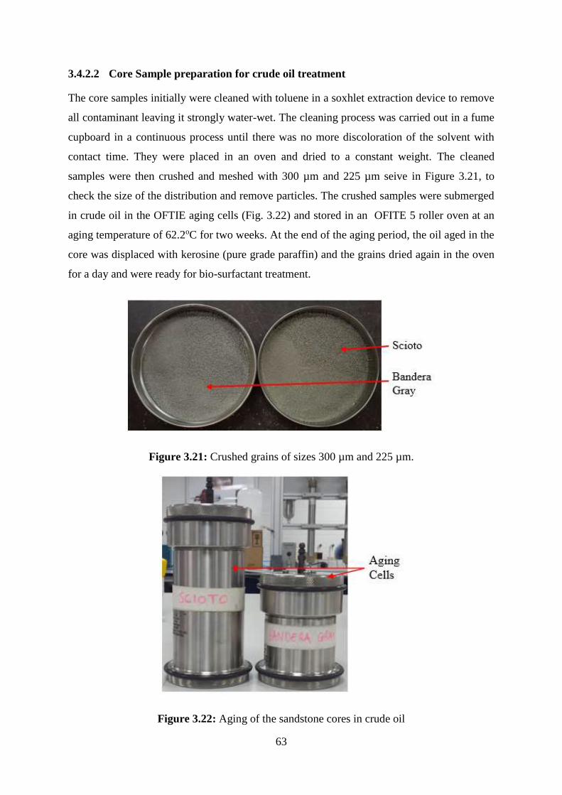
63

3.4.2.2 Core Sample preparation for crude oil treatment

The core samples initially were cleaned with toluene in a soxhlet extraction device to remove

all contaminant leaving it strongly water-wet. The cleaning process was carried out in a fume

cupboard in a continuous process until there was no more discoloration of the solvent with

contact time. They were placed in an oven and dried to a constant weight. The cleaned

samples were then crushed and meshed with 300 µm and 225 µm seive in Figure 3.21, to

check the size of the distribution and remove particles. The crushed samples were submerged

in crude oil in the OFTIE aging cells (Fig. 3.22) and stored in an OFITE 5 roller oven at an

aging temperature of 62.2oC for two weeks. At the end of the aging period, the oil aged in the

core was displaced with kerosine (pure grade paraffin) and the grains dried again in the oven

for a day and were ready for bio-surfactant treatment.

Figure 3.21: Crushed grains of sizes 300 µm and 225 µm.

Figure 3.22: Aging of the sandstone cores in crude oil

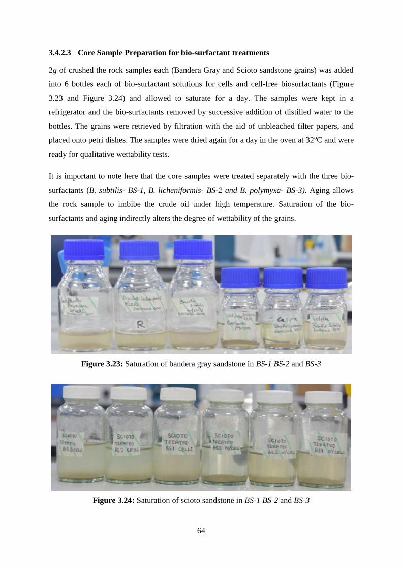
64

3.4.2.3 Core Sample Preparation for bio-surfactant treatments

2g of crushed the rock samples each (Bandera Gray and Scioto sandstone grains) was added

into 6 bottles each of bio-surfactant solutions for cells and cell-free biosurfactants (Figure

3.23 and Figure 3.24) and allowed to saturate for a day. The samples were kept in a

refrigerator and the bio-surfactants removed by successive addition of distilled water to the

bottles. The grains were retrieved by filtration with the aid of unbleached filter papers, and

placed onto petri dishes. The samples were dried again for a day in the oven at 32oC and were

ready for qualitative wettability tests.

It is important to note here that the core samples were treated separately with the three bio-

surfactants (B. subtilis- BS-1, B. licheniformis- BS-2 and B. polymyxa- BS-3). Aging allows

the rock sample to imbibe the crude oil under high temperature. Saturation of the bio-

surfactants and aging indirectly alters the degree of wettability of the grains.

Figure 3.23: Saturation of bandera gray sandstone in BS-1 BS-2 and BS-3

Figure 3.24: Saturation of scioto sandstone in BS-1 BS-2 and BS-3

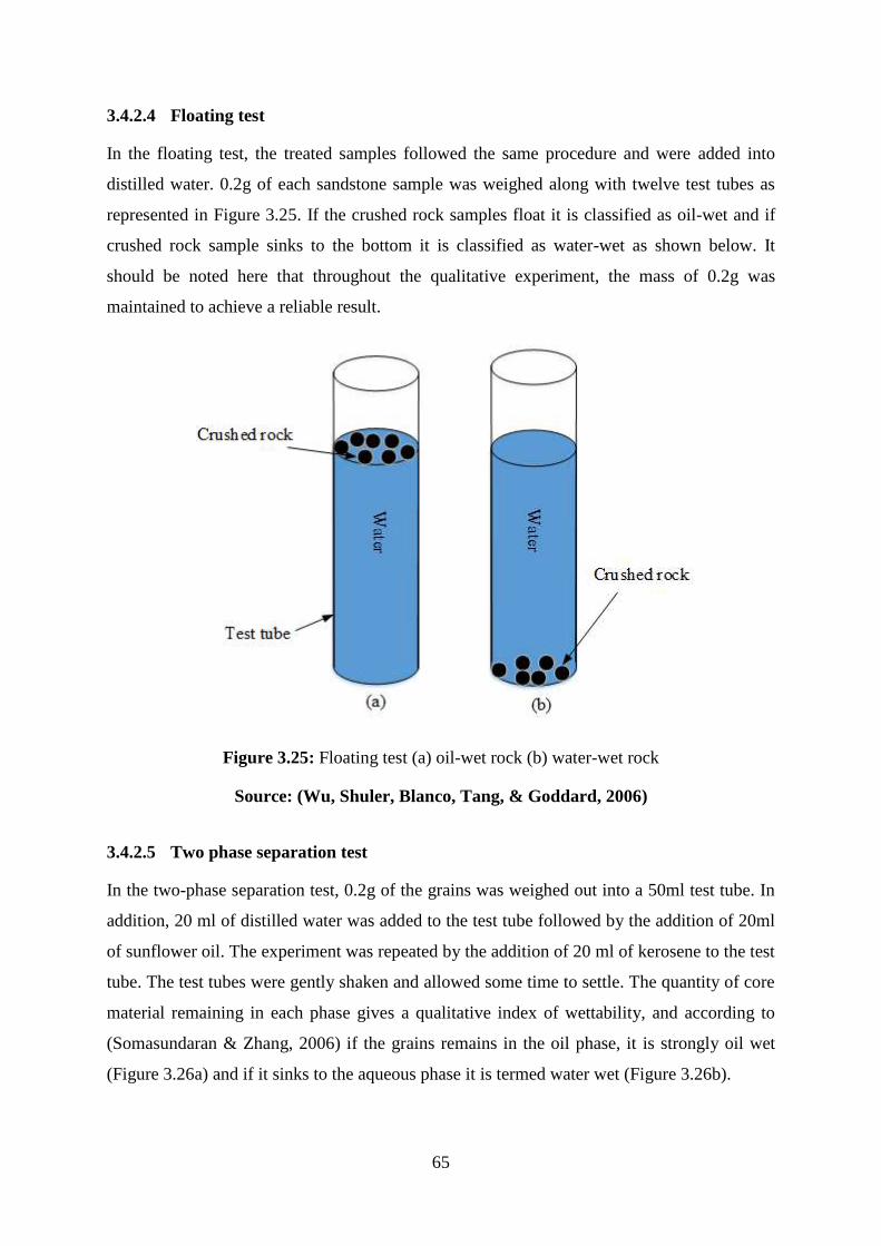
65

3.4.2.4 Floating test

In the floating test, the treated samples followed the same procedure and were added into

distilled water. 0.2g of each sandstone sample was weighed along with twelve test tubes as

represented in Figure 3.25. If the crushed rock samples float it is classified as oil-wet and if

crushed rock sample sinks to the bottom it is classified as water-wet as shown below. It

should be noted here that throughout the qualitative experiment, the mass of 0.2g was

maintained to achieve a reliable result.

Figure 3.25: Floating test (a) oil-wet rock (b) water-wet rock

Source: (Wu, Shuler, Blanco, Tang, & Goddard, 2006)

3.4.2.5 Two phase separation test

In the two-phase separation test, 0.2g of the grains was weighed out into a 50ml test tube. In

addition, 20 ml of distilled water was added to the test tube followed by the addition of 20ml

of sunflower oil. The experiment was repeated by the addition of 20 ml of kerosene to the test

tube. The test tubes were gently shaken and allowed some time to settle. The quantity of core

material remaining in each phase gives a qualitative index of wettability, and according to

(Somasundaran & Zhang, 2006) if the grains remains in the oil phase, it is strongly oil wet

(Figure 3.26a) and if it sinks to the aqueous phase it is termed water wet (Figure 3.26b).

66

Figure 3.26: Two phase separation test (a) oil-wet rock (b) water-wet rock

Source: (Somasundaran & Zhang, 2006)

Error and Accuracy

i. Sampling errors have been accounted for by repeating each set of experiment over

three uniquely measured samples, following the same procedures.

ii. The grain size and weight may have had influence on the buoyancy force of the fluid.

3.5 Phase-IV: Core Flooding

The core flooding experiment will be performed to evaluate the effectiveness of bio-

surfactant treatments in altering wettability of sandstone reservoirs. Sandstone reservoir core

will be used in core flood tests at simulated reservoir conditions. For a treatment to be

considered for core flooding, it must be stable at ambient and reservoir conditions to avoid

damaging the rock permeability. Therefore, the treatment solution should not polymerise;

should not precipitate before or during injection into the core, or upon heating; and it should

not cause any unwanted reaction in the core with either rock minerals or other fluid(s)

initially in the core.


A major part of the experimental work related to this study was the bio-surfactant flooding,

which was carried out using Figure 3.27, the CoreLab UFS-200 core flooding system student

67

module apparatus, located within the Department of Petroleum Engineering at The University

of Salford. The equipment is configured for two phase liquid displacements under unsteady

state or steady-state conditions and single phase gas steady-state experiments. For this study,

the unsteady state liquid displacement method was adopted due to the displacement of each

fluid utilised at a time. The flow path of the core flooding experiment can be seen in a simple

schematic shown in Figure 3.28.

3.5.1.1 Description of CoreLab UFS-200

The system is rated to 5,000 psig confining pressure, 3,500 psig pore pressure at room

temperature. An integral part of the system is the SmartFlood software and computer data-

acquisition-and-control system hardware, which provides on-screen display of all measured

values (pressures, temperatures, volumes etc.), automatic logging of test data to a computer

data file, alarms, graphing, calculation of permeability, operate the pump delivery system for

the start/stop of fluid flow and control of the flow rate. The major components of the core

flooding apparatus is further explained in details to highlight their mode of operation and

their importance in effectively performing the experiments. The entire system can be divided

into four sections; to include the core holder, fluid injection system, data acquisition system

and the collection tube.

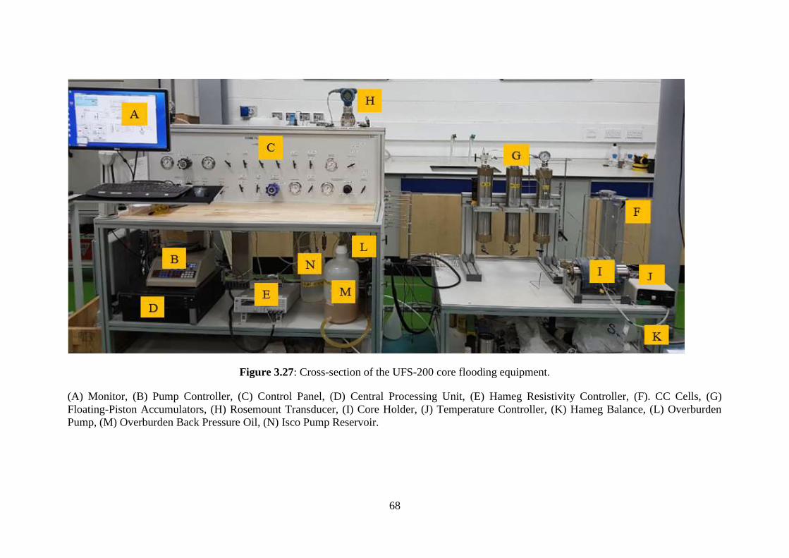
68

Figure 3.27: Cross-section of the UFS-200 core flooding equipment.

(A) Monitor, (B) Pump Controller, (C) Control Panel, (D) Central Processing Unit, (E) Hameg Resistivity Controller, (F). CC Cells, (G)

Floating-Piston Accumulators, (H) Rosemount Transducer, (I) Core Holder, (J) Temperature Controller, (K) Hameg Balance, (L) Overburden

Pump, (M) Overburden Back Pressure Oil, (N) Isco Pump Reservoir.

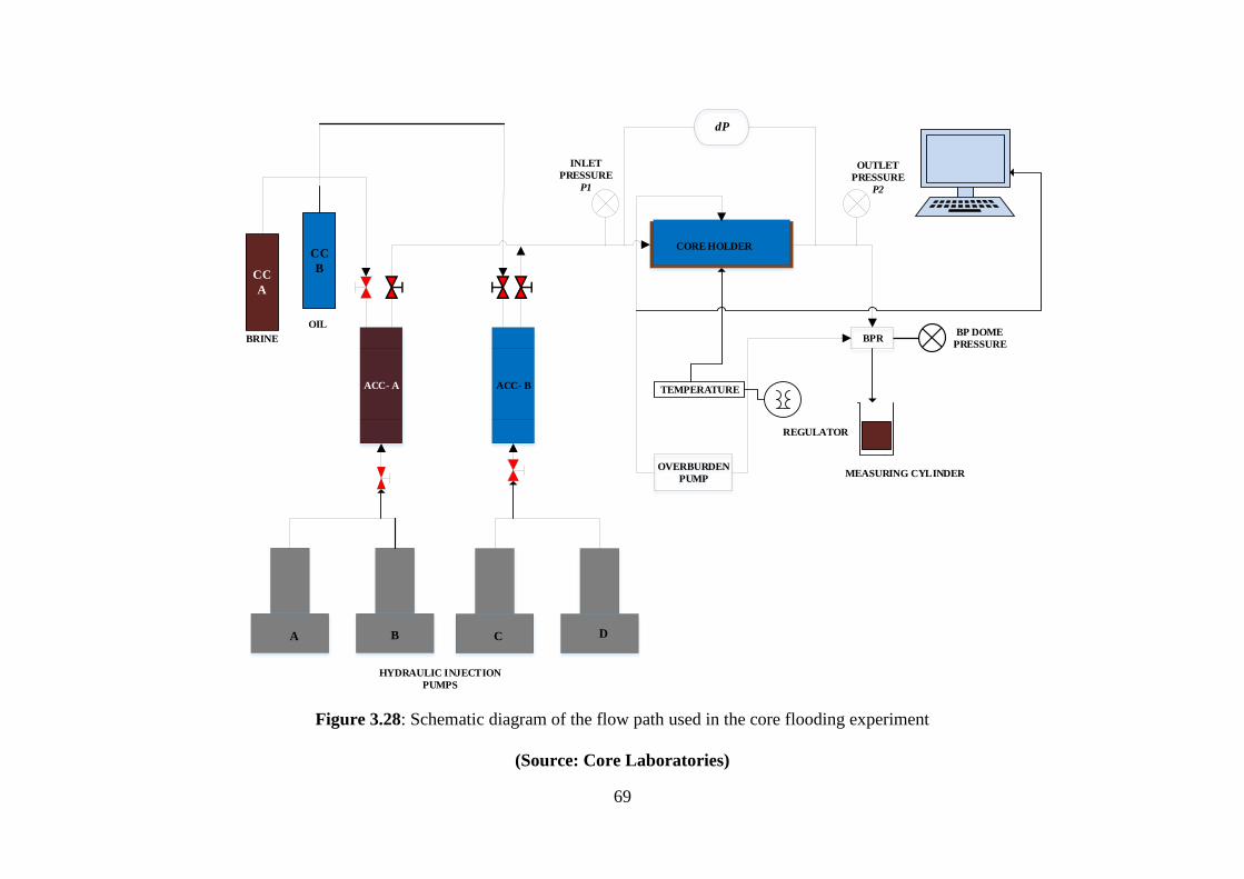
69

OVERBURDEN

PUMP

ACC- A ACC- B

CORE HOLDER

dP

BP DOME

PRESSUREBPR

INLET

PRESSURE

P1

OUTLET

PRESSURE

P2

HYDRAULIC INJECTION

PUMPS

A B C D

CC

A

CC

B

BRINE

OIL

MEASURING CYLINDER

TEMPERATURE

REGULATOR

Figure 3.28: Schematic diagram of the flow path used in the core flooding experiment

(Source: Core Laboratories)

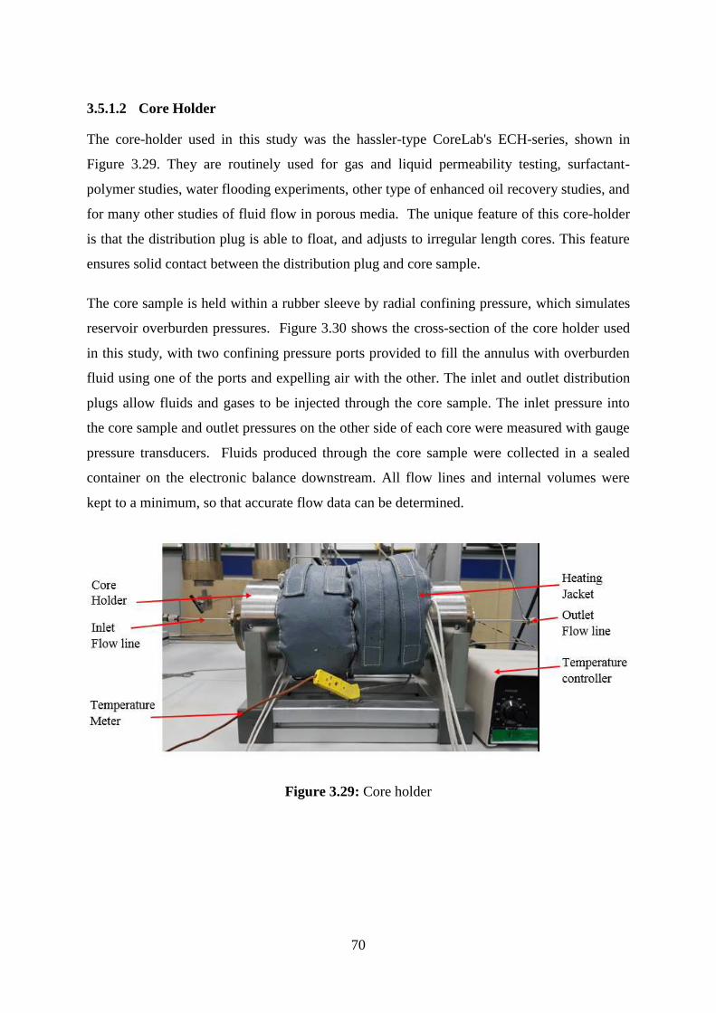
70

3.5.1.2 Core Holder

The core-holder used in this study was the hassler-type CoreLab's ECH-series, shown in

Figure 3.29. They are routinely used for gas and liquid permeability testing, surfactant-

polymer studies, water flooding experiments, other type of enhanced oil recovery studies, and

for many other studies of fluid flow in porous media. The unique feature of this core-holder

is that the distribution plug is able to float, and adjusts to irregular length cores. This feature

ensures solid contact between the distribution plug and core sample.

The core sample is held within a rubber sleeve by radial confining pressure, which simulates

reservoir overburden pressures. Figure 3.30 shows the cross-section of the core holder used

in this study, with two confining pressure ports provided to fill the annulus with overburden

fluid using one of the ports and expelling air with the other. The inlet and outlet distribution

plugs allow fluids and gases to be injected through the core sample. The inlet pressure into

the core sample and outlet pressures on the other side of each core were measured with gauge

pressure transducers. Fluids produced through the core sample were collected in a sealed

container on the electronic balance downstream. All flow lines and internal volumes were

kept to a minimum, so that accurate flow data can be determined.

Figure 3.29: Core holder

71

Figure 3.30: A cross-section of the hassle core holder

(Source: Core Laboratory)

3.5.1.3 The Injection System

3.5.1.3.1 Floating-Piston Accumulators

CoreLab floating-piston accumulators are rated for 5,000 psig pressure and 350°F (177°C)

temperature. The accumulator volumes are 500 cc each and provide for injecting fluids

without allowing the fluid to come in contact with the metering pump (Figure 3.31). In this

study, accumulator A (oil) and accumulator B (brine/bio-surfactant) were used in saturation

and the flooding process. The CC-series reservoirs were used for the storage and transfer of

test fluids. The test fluids of known volume were fed into the CC-cells A/B in Figure 3.32, by

opening the top assembly and then opening the appropriate valve at the bottom the CC-cell,

the fluid was injected into the desired accumulator with the aid of the ISCO pump.

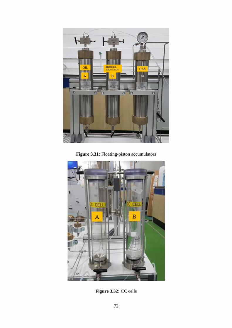
72

Figure 3.31: Floating-piston accumulators

Figure 3.32: CC cells

73

3.5.1.3.2 Metering Pump and Overburden Pressure Pump

The ISCO model 500D is a two-barrel metering pump system which has a flow rate range

adjustable from 0 to 200 ml/min and a maximum pressure rating of 3,750 psig (Figure 3.33).

It’s pump’s limits are set to turn off itself before it reaches too high of a pressure. The ISCO

pump can be controlled by the pump controller as seen in Figure 3.27-B, and can be used to

inject brine or test fluid into the core sample via the floating piston accumulator. The simple

procedure here is to close the valves to the confining pressure system and release the pressure

in the ISCO pump. Then open the valve to accumulator and the valve at the bottom of the

accumulator. Also, open the purge valve at the top of the accumulator to drain all air out of

the flow lines. With a properly filled accumulator, brine or other test liquid can now be

injected into the core sample.

Figure 3.33: Metering Isco pumps

Figure 3.34, represents the overburden (confining) pressure pump is a hydraulic pump, with a

maximum pressure output of 10,000 psig. The maximum overburden pressure rating of the

core holder and system is 5,000 psig. It functions by gradually pumping hydraulic oil into the

annulus of the core holder to build up the desired overburden confining pressure as well as

the back pressure.

74

Figure 3.34: Overburden pump and relevant reservoirs

3.5.1.4 The Collection System

As part of the process during initializing the equipment, the hameg balance is turned on and

tared (zeroed). The leak-off fluids produced through the core during experimental runs can be

collected by the electronic balance at the outlet of the core’s BPR. The liquids flow through

the back-pressure regulator (BPR) and into a sealed container on the balance (Figure 3.25).

The produced fluid is then poured into a measuring cylinder and allowed to settled before

taking any measurements.

Figure 3.35: Hameg electronic balance

75

3.5.1.5 The Data Acquisition and Control System.

The data acquisition system consists of a personal computer and the control system

SmartFlood software communicates to the UFS system through Ethernet. The entire hardware

components and sensors of the system is controlled and monitored with the computer by

providing on-screen display of all measured values (flow rates, pressures, temperature etc.),

remote control of flow rates, automatic logging of test data to a data file, alarms, calculations

and graphing as seen in Figure 3.27-A. A major advantage of this system is that it provides a

means to remotely acquire and record test results. The data logging features in the software

relieves the operator of much of the tedious, time-consuming setup and data recording that

used to be required when running tests.

3.5.1.6 Back-Pressure Regulator, Pressure Gauges, Air Actuated Valves, and Pressure

Transducers

The CoreLab back-pressure regulator controls the back (outlet) pressure. It is rated for a

maximum working pressure of 5,000 psig, and is a dome-loaded type which controls the back

pressure to whatever pressure is supplied to its dome. For this system, 2.5-inch-dial pressure

gauges are used to monitor the Overburden Pressure and the BPR Dome Pressure. The

pressure range on these gauges is 15,000-psig full scale. A 160-psi gauge is provided to

monitor the main inlet air going to the pump and air actuated valves. The system uses

Vindum, CV series High Pressure (10,000 psig) three-way valves, which can be operated

remotely via the SmartFlood software. The Rosemount transducer measures the differential

pressure across the core holder.

5.5.1.7 Materials

The following listed materials were used in successfully performing the bio-

flooding/waterflooding experiments.

i. Bandera Gray core sample, as described in Section 3.4.2.1

ii. Crude oil sample, as described in Table 3.3

iii. BS-2 supernatant biosurfactant

iv. Distilled water

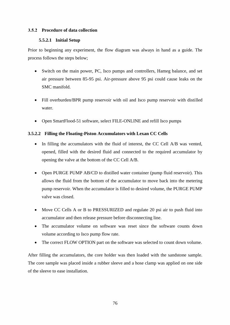
76


5.5.2.1 Initial Setup

Prior to beginning any experiment, the flow diagram was always in hand as a guide. The

process follows the steps below;

Switch on the main power, PC, Isco pumps and controllers, Hameg balance, and set

air pressure between 85-95 psi. Air-pressure above 95 psi could cause leaks on the

SMC manifold.

Fill overburden/BPR pump reservoir with oil and Isco pump reservoir with distilled

water.

Open SmartFlood-51 software, select FILE-ONLINE and refill Isco pumps

3.5.2.2 Filling the Floating-Piston Accumulators with Lexan CC Cells

In filling the accumulators with the fluid of interest, the CC Cell A/B was vented,

opened, filled with the desired fluid and connected to the required accumulator by

opening the valve at the bottom of the CC Cell A/B.

Open PURGE PUMP AB/CD to distilled water container (pump fluid reservoir). This

allows the fluid from the bottom of the accumulator to move back into the metering

pump reservoir. When the accumulator is filled to desired volume, the PURGE PUMP

valve was closed.

Move CC Cells A or B to PRESSURIZED and regulate 20 psi air to push fluid into

accumulator and then release pressure before disconnecting line.

The accumulator volume on software was reset since the software counts down

volume according to Isco pump flow rate.

The correct FLOW OPTION part on the software was selected to count down volume.

After filling the accumulators, the core holder was then loaded with the sandstone sample.

The core sample was placed inside a rubber sleeve and a hose clamp was applied on one side

of the sleeve to ease installation.

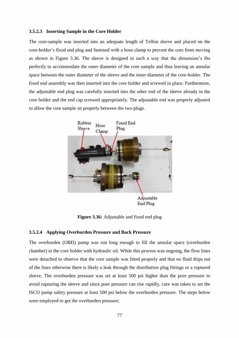
77

3.5.2.3 Inserting Sample in the Core Holder

The core-sample was inserted into an adequate length of Telfon sleeve and placed on the

core-holder’s fixed end plug and fastened with a hose clamp to prevent the core from moving

as shown in Figure 3.36. The sleeve is designed in such a way that the dimension’s fits

perfectly to accommodate the outer diameter of the core sample and thus leaving an annular

space between the outer diameter of the sleeve and the inner diameter of the core-holder. The

fixed end assembly was then inserted into the core holder and screwed in place. Furthermore,

the adjustable end plug was carefully inserted into the other end of the sleeve already in the

core holder and the end cap screwed appropriately. The adjustable end was properly adjusted

to allow the core sample sit properly between the two plugs.

Figure 3.36: Adjustable and fixed end plug

3.5.2.4 Applying Overburden Pressure and Back Pressure

The overburden (OBD) pump was run long enough to fill the annular space (overburden

chamber) in the core holder with hydraulic oil. While this process was ongoing, the flow lines

were detached to observe that the core sample was fitted properly and that no fluid drips out

of the lines otherwise there is likely a leak through the distribution plug fittings or a ruptured

sleeve. The overburden pressure was set at least 500 psi higher than the pore pressure to

avoid rupturing the sleeve and since pore pressure can rise rapidly, care was taken to set the

ISCO pump safety pressure at least 500 psi below the overburden pressure. The steps below

were employed to get the overburden pressure;

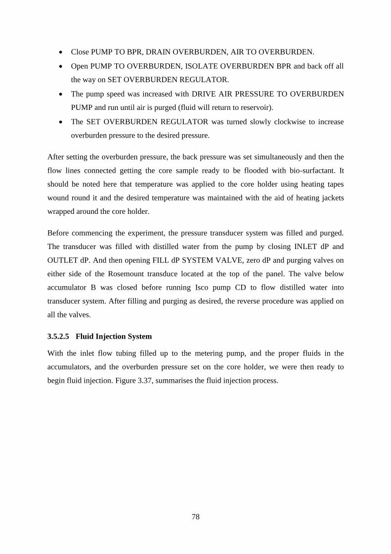
78

Close PUMP TO BPR, DRAIN OVERBURDEN, AIR TO OVERBURDEN.

Open PUMP TO OVERBURDEN, ISOLATE OVERBURDEN BPR and back off all

the way on SET OVERBURDEN REGULATOR.

The pump speed was increased with DRIVE AIR PRESSURE TO OVERBURDEN

PUMP and run until air is purged (fluid will return to reservoir).

The SET OVERBURDEN REGULATOR was turned slowly clockwise to increase

overburden pressure to the desired pressure.

After setting the overburden pressure, the back pressure was set simultaneously and then the

flow lines connected getting the core sample ready to be flooded with bio-surfactant. It

should be noted here that temperature was applied to the core holder using heating tapes

wound round it and the desired temperature was maintained with the aid of heating jackets

wrapped around the core holder.

Before commencing the experiment, the pressure transducer system was filled and purged.

The transducer was filled with distilled water from the pump by closing INLET dP and

OUTLET dP. And then opening FILL dP SYSTEM VALVE, zero dP and purging valves on

either side of the Rosemount transduce located at the top of the panel. The valve below

accumulator B was closed before running Isco pump CD to flow distilled water into

transducer system. After filling and purging as desired, the reverse procedure was applied on

all the valves.

3.5.2.5 Fluid Injection System

With the inlet flow tubing filled up to the metering pump, and the proper fluids in the

accumulators, and the overburden pressure set on the core holder, we were then ready to

begin fluid injection. Figure 3.37, summarises the fluid injection process.

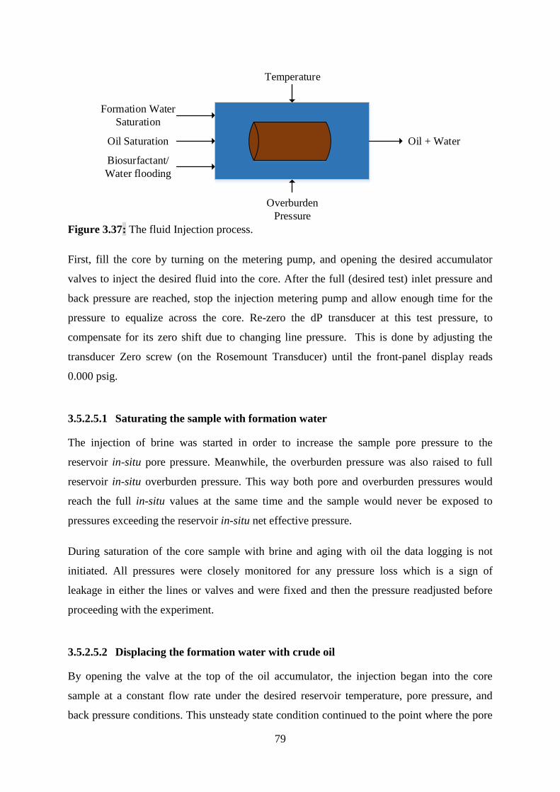
79

Formation Water

Saturation

Biosurfactant/

Water flooding

Oil Saturation Oil + Water

Temperature

Overburden

Pressure Figure 3.37: The fluid Injection process.

First, fill the core by turning on the metering pump, and opening the desired accumulator

valves to inject the desired fluid into the core. After the full (desired test) inlet pressure and

back pressure are reached, stop the injection metering pump and allow enough time for the

pressure to equalize across the core. Re-zero the dP transducer at this test pressure, to

compensate for its zero shift due to changing line pressure. This is done by adjusting the

transducer Zero screw (on the Rosemount Transducer) until the front-panel display reads

0.000 psig.

3.5.2.5.1 Saturating the sample with formation water

The injection of brine was started in order to increase the sample pore pressure to the

reservoir in-situ pore pressure. Meanwhile, the overburden pressure was also raised to full

reservoir in-situ overburden pressure. This way both pore and overburden pressures would

reach the full in-situ values at the same time and the sample would never be exposed to

pressures exceeding the reservoir in-situ net effective pressure.

During saturation of the core sample with brine and aging with oil the data logging is not

initiated. All pressures were closely monitored for any pressure loss which is a sign of

leakage in either the lines or valves and were fixed and then the pressure readjusted before

proceeding with the experiment.

3.5.2.5.2 Displacing the formation water with crude oil

By opening the valve at the top of the oil accumulator, the injection began into the core

sample at a constant flow rate under the desired reservoir temperature, pore pressure, and

back pressure conditions. This unsteady state condition continued to the point where the pore

80

pressure almost equal the back pressure thus initiating a flow. At this point, brine was

produced which was collected into a measuring cylinder and with continued flow a

breakthrough was achieved (a mixture of oil and brine) and then only oil started flowing.

Once the breakthrough was achieved, the time and other pressure conditions were noted. The

oil injection continued until 3 pore volumes were produced at which point the core should be

fully saturated with oil and then the produced water measured. However, in order to be

certain of full oil saturation, the sample was left for 24-hours to age under reservoir in-situ P-

T conditions, while all pressures were monitored for any fluctuations and then adjusted

accordingly.

3.5.2.5.3 Displacing the crude oil with distilled water (waterflooding)

This flooding process was carried out as a control measure to set a benchmark of the oil

recovered while comparing the outcome with the bio-surfactant recovery. Also, it was

necessary to determine the best flow rate that would give the maximum oil recovery by

carrying out repetitive test runs at different flow rates. During the injection of distilled water,

the overburden pressure and back pressure was maintained. The pore pressure however

increased to a point where flow was initiated until there was a breakthrough of water. The

low flow rate was necessary to avoid a viscous fingering through the core, therefore

displacing more of the oil. The amount of oil recovered was then measured and the residual

oil left behind was calculated and used as the benchmark for this study.

3.5.2.5.4 Displacing the crude oil with bio-surfactant (bioflooding)

At the start of the distilled water/bio-surfactant flooding, the data logging is initiated with 10

seconds logging interval. To be able to achieve one of the aims of this study, the basic

flooding procedure was slightly modified and extended with repeatability experiment carried

during the procedure above, certain parameters which would be used during data

analysis/interpretation, were recorded against time. These parameters included the brine and

oil production and/or injection volumes and flowrates, core holder inlet and outlet pressures,

breakthrough time and stabilised conditions e.g. differential pressure.

3.5.2.6 End Test

The back pressure was released by opening BPR VENT

81

Release (back off on SET OVERBURDEN regulator) and drain overburden to

remove the core (open AIR TO OVERBURDEN and DRAIN OVERBURDEN).

All the lines were then cleaned by flowing through with either distilled water and/or soap as

needed.

Errors and Accuracy

i. Re-zero the dP transducer at the test pressure, to compensate for its zero-shift due to

changing line pressure. This is done by adjusting the transducer Zero screw (on the

Rosemount Transducer) until the front-panel display reads 0.000 psig.

ii. All measurements were made in triplicate at elevated temperature (60±2)oC and

flowrate (0.25 ml/min), and the average values were reported.

3.6 Chapter Summary

The main points of the experimental process of this chapter may be summarised as follows:

The recovering of pure cultures:

Three selected microbial strains were retrieved from freeze dried condition.

These microbes were grown on selected media and LB agar

The growth was carried out on different temperatures, and a phenotypic characteristic

which is gram-stain was performed to determine if the microbes were gram-positive

bacterial.

Quantitative screening:

Heavy oil was utilised in a pendant drop system, comprising of synthetic formation

water and the produced biosurfactants, to observe for reduction in IFT and contact

angle, in the liquid-liquid phase.

This sets of experiments were performed at varying temperatures and pressures, for

both supernatant biosurfactants and biosurfactants with cells.

Qualitative analysis:

Two sandstones of different permeability’s were used here to see how effective these

microbes could be in affecting their pore spaces.

82

Two qualitative tests (floating and two-phase separation) were used here, to determine

the effectiveness of the core cleaning, as well the effectiveness of the biosurfactants in

changing the wettability of the crude oil aged crushed rock.

Core flooding:

The core flood test was carried out on Bandera Gray sandstone at simulated reservoir

conditions, using supernatant BS-2 biosurfactant, and also waterflooding was

performed, for a direct comparison of the oil recovered.

The next chapter describes the experimental analysis and results obtained from this study.

83

Chapter 4

4 Result and Discussions

4.1 Overview

This chapter introduces the results obtained from the experimental investigation conducted

according to the equipment, material selection and procedure, set out in Figure 3.1, which is

in line with the original target of this investigation in utilising microbial surfactants to

mobilize residual oil from mature reservoir and increase production. The results are

categorised into four phases in which the experimental sequence followed.

Phase I: Microbial culture: Section 4.2 highlights the condition for effectively

growing the strains in producing the required biosurfactant and determination of

phenotypic characteristics of the strains to verify that they are gram-positive bacterials

as will be detailed in Section 4.2.1. The extraction of the produced biosurfactants is

given in Section 4.2.3. The qualititative results have been illustrated in relation to the

microbial culture.

Phase II: Interfacial tension/contact angle measurements were conducted

quantitatively using Pendant DROPimage technique as detailed in Section 3.3.3.2 for

both cells and cell-free cultures of BS-1, BS-2 and BS-3. The measurement of the

effect of biosurfactants in reducing the IFT/contact angle of heavy crude oil is a first

step towards achieving enhance recovery.

Phase III: Qualitative wettability tests. In Section 4.4 the effects of the biosurfactants

can be seen on how it has been able to effectively change the rock chemistry, thus

altering the wettability of the crude oil aged crushed rock. This qualitative process

follows the principle of floatation in two forms, which includes the floating test in

Section 4.4.2 and two-phase seperation test in Section 4.4.3.

Phase IV: Coreflooding in enhancing recovery in heavy oil reservoirs. In Section 3.5,

the unsteady state liquid displacement was utilised during the bioflooding process,

and the biosurfactant that gave the best IFT reduction was then used to perform the

tertiary recovery, since it could be a potential candidate for EOR.

84

4.2 Phase I - Microbial Culture

Culture and Growth

The isolation of pure cultures from freeze dried condition to recover the cells is summarized

in Figure 4:1 below, showing the growth of bacteria on nutrient agar and liquid broth. The

strains used were grown for 48 hours at 30oC and 37oC respectively. It was observed that

there was faster growth at 37oC in the first 24 hours for all three strains, and more visible

growth was seen at both temperatures after 48 hours. However, the growth of type strain

DSM 740, was minimal, even after 2 days, and the weak observation of growth was taken as

a positive result as shown in Figure 4.2 and Figure 4.3.

Phenotypic Characteristics

The observable physical characteristics of the microbes used in this study were determined to

confirm that the selected bacterial were gram positive.

4.2.2.1 Colony Morphology of Microorganisms

In this study, the strains used were proven to be gram-positive bacterial, B. subtilis (Perez,

Abanes-De Mello, & Pogliano, 2000), B. licheniformis (Jeong et al., 2011), and B.

Paenibacillus polymyxa. The colonies of B. licheniformis appeared whitish at 37oC like

lichens or a big wad of snot that grow on rocks, about 1 µm in diameter. After 48 hours of

incubating B. subtilis at 37oC, the cream-colored colonies formed appeared thick and opaque

with lobate margins about 2.0-3.0/0.7-0.8 µm. In addition, P. polymyxa, 0.3 by 0.6 µm in size

produced thin-pale colonies on agar. These strains are motile by peritrichous flagella

(containing protein) and their vegetative cell were not destroyed because they form a sub-

terminal or paracentral spore. These features can be seen in Figure 4.3.

85

Figure 4.1: Isolation of pure cultures and growth of bacteria

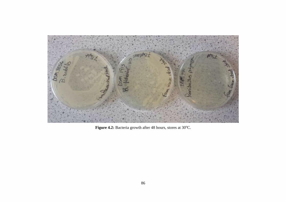
86

Figure 4.2: Bacteria growth after 48 hours, stores at 30oC.

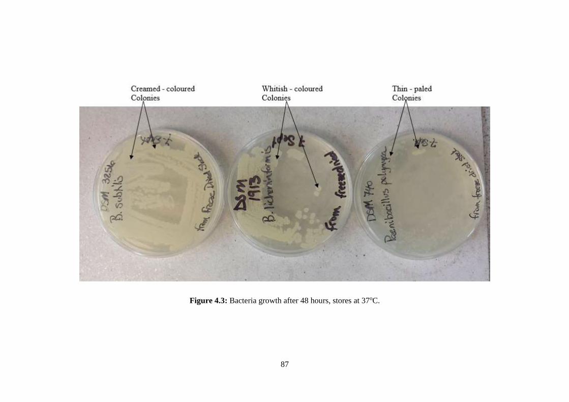
87

Figure 4.3: Bacteria growth after 48 hours, stores at 37oC.

88

4.2.2.2 Gram Staining

It was observed that all three strains of bacteria selected for this study were not decolorised

by alcohol and remained purple, when the cells were observed under light microscope, as

seen in Figure 4.4. This procedure has helped to determine the presence of bacteria in the

selected strains, and has proven that, all three strains are gram-positive bacteria, and accepted

to be gram-positive cells. The bacterials were able to retain the crystal violet dye that was

used to stain the cells, because the gram-positive bacteria have a very thick cell wall made of

protein called peptidoglycan.

PCR Amplification

PCR is sometimes refered to as molecular photocopying, which is used to amplify small

segments of DNA into larger ones. It was necessary to carry out this process, due to the

sample strains having small amount of DNA to characterise it by sequencing. Larger amounts

of DNA mean more accurate and realiable results.

The sequence of each of the bacterium was compared with the 16S rRNA sequence in the

Generious R9 library (v 9.15) . Upon comparison, the software provided a potential ID for the

unknown bacterial species. The Generious R9 ID 16S rRNA library (v 9.15) included over

1489 validated 16S rRNA sequences for each bacterium (NCBI, 2016). All sequences and

strains were carefully checked and quality controlled to achieve maximum realibility.

Identically colored boxes as seen in Figure 4.5, indicates the selected bacterial belonging to

the same gene family in which they were compared with. The different colors represents the

different sequence idientities which can easily be observed by the broken portions. The

complete sequence alignment and comparison between the the strains and the reference

strains can futher be seen in Appendix B.

Serial Dilutions

The sequential dilutions were used to reduce the dense culture of the cells to a more usable

concentration. It helped to determine the number of bacteria per unit volume in the original

culture, and determination of the culture density in cells per ml. B. subtilis strain as a

representative example and were formed in 10-1 to 10-6 dilutions after 48 hours of incubation

as seen in Figure 4.6. Each countable colony contains thousands of individual bacteria. The

simple calculation is thus presented below.

89

The concentration of microscopic cells in a sample of B. subtilis can be calculated thus;

𝑁𝑢𝑚𝑏𝑒𝑟 𝑜𝑓 𝑐𝑜𝑙𝑜𝑛𝑖𝑒𝑠 𝑜𝑛 𝑝𝑙𝑎𝑡𝑒 × 𝑟𝑒𝑐𝑖𝑝𝑟𝑜𝑐𝑎𝑙 𝑜𝑓 𝑑𝑖𝑙𝑢𝑡𝑖𝑜𝑛 𝑜𝑓 𝑠𝑎𝑚𝑝𝑙𝑒 =

𝑛𝑢𝑚𝑏𝑒𝑟 𝑜𝑓 𝑏𝑎𝑐𝑡𝑒𝑟𝑖𝑎/𝑚𝑙 (4.1)

For example, there are 52 colonies on the plate of 1/1,000,000 dilution, then the count is:

52 × 1000000 = 52, 000, 000 𝑏𝑎𝑐𝑡𝑒𝑟𝑖𝑎/𝑚𝑙 𝑖𝑛 𝑠𝑎𝑚𝑝𝑙𝑒

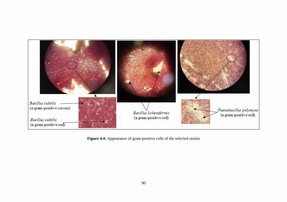
90

Figure 4.4: Appearance of gram-positive cells of the selected strains

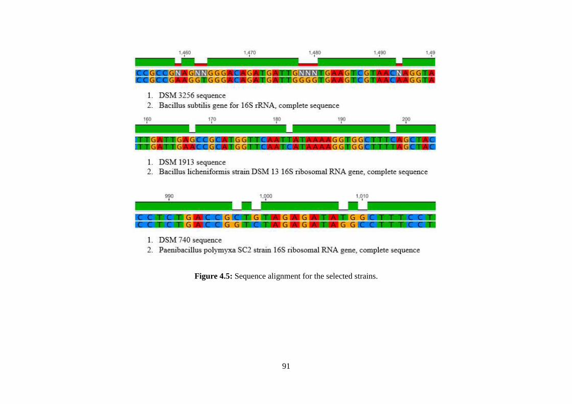
91

Figure 4.5: Sequence alignment for the selected strains.

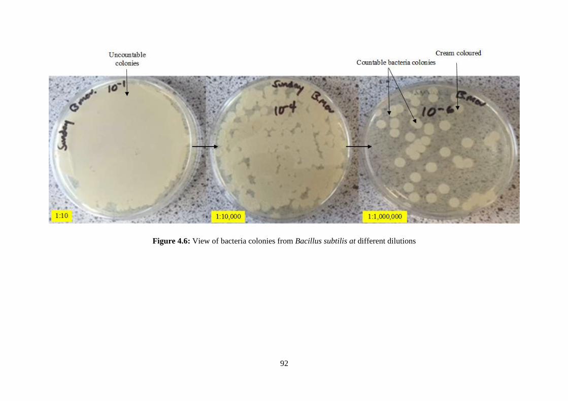
92

Figure 4.6: View of bacteria colonies from Bacillus subtilis at different dilutions

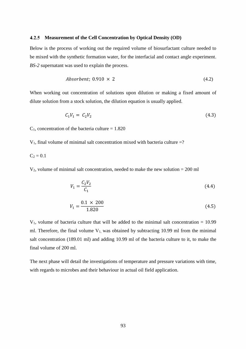
93

Measurement of the Cell Concentration by Optical Density (OD)

Below is the process of working out the required volume of biosurfactant culture needed to

be mixed with the synthetic formation water, for the interfacial and contact angle experiment.

BS-2 supernatant was used to explain the process.

𝐴𝑏𝑠𝑜𝑟𝑏𝑒𝑛𝑡; 0.910 × 2 (4.2)

When working out concentration of solutions upon dilution or making a fixed amount of

dilute solution from a stock solution, the dilution equation is usually applied.

𝐶1𝑉1 = 𝐶2𝑉2 (4.3)

C1, concentration of the bacteria culture = 1.820

V1, final volume of minimal salt concentration mixed with bacteria culture =?

C2 = 0.1

V2, volume of minimal salt concentration, needed to make the new solution = 200 ml

𝑉1 =𝐶2𝑉2

𝐶1 (4.4)

𝑉1 =0.1 × 200

1.820 (4.5)

V1, volume of bacteria culture that will be added to the minimal salt concentration = 10.99

ml. Therefore, the final volume V1, was obtained by subtracting 10.99 ml from the minimal

salt concentration (189.01 ml) and adding 10.99 ml of the bacteria culture to it, to make the

final volume of 200 ml.

The next phase will detail the investigations of temperature and pressure variations with time,

with regards to microbes and their behaviour in actual oil field application.

94

4.3 Phase II - Interfacial Tension and Contact Angle

Interfacial Tension Measurements

The measurement of interfacial tension is an integral part of this investigation as the

application of biosurfactant can aggregate at the interfaces between fluids having different

polarities, such as water and oil, leading to the reduction in interfacial tension (El-Sheshtawy,

Aiad, Osman, Abo-ELnasr, & Kobisy, 2015; Fang et al., 2007). One of the major

considerations, with enhanced oil recovery, is how much the injected bacteria can stimulate

the production of additional oil from reservoirs. Usually, this is achieved by the addition of

nutrients during water injection. The reduction in interfacial tension is possible by

stimulating the growth of bacteria at an oil/water interface, which in turn can aid the recovery

of oil. The effects of temperature and pressure on interfacial activity helps to show the

behaviour of liquids during interfacial tension measurements. And with the help of densitiy

difference between liquids, interfacial tension is easily calculated by the pendant drop

method.

Previously, Lin, Chen, Xyu, & Wang, (1995) concluded that after experimenting with

air/water and fluid/fluid interfaces, the measured IFT is drop dependent. In this present study,

it is demonstrated that there is a reasonable and clear impact of the drop size on the

measurment of the IFT. The bigger the drop the more reasonable it is in estimating the IFT by

the pendant drop technique, in light of the fact that with this there is higher accuracy, in the

image edge detection process. This perception concurs with Yang, Wei, & Lin, (2007) who

likewise contempleted the impact of drop size on the IFT and adsorption of surfactants, and it

demonstrates the high accuracy with which the drop coordinates, must be resolved and not

just rely upon the numerical treatment of the data, but also on the experimental data itself.

In this present study, a total of three hundred and thirty nine (285) IFT measurements were

performed at different temperatures and pressure ranges from 0.15 MPa to 13.89 MPa. The

interfacial tension data generated from the analysis are discussed below.

The control experiment for crude oil/distilled water system was conducted using the

equipment and procedure that were described in the previous Chapter 3. The results shows

that there are variations between the interfacial tension with the temperatures. The expected

decrease of interfacial tension from 56.95 to 29.47 mN/m, between 26oC and 75oC, for raw

crude oil/distilled water system is typified in Figure 4.7. A similar trend was also reported by

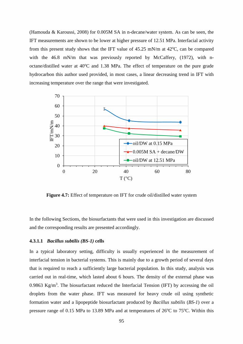
95

(Hamouda & Karoussi, 2008) for 0.005M SA in n-decane/water system. As can be seen, the

IFT measurements are shown to be lower at higher pressure of 12.51 MPa. Interfacial activity

from this present study shows that the IFT value of 45.25 mN/m at 42oC, can be compared

with the 46.8 mN/m that was previously reported by McCaffery, (1972), with n-

octane/distilled water at 40oC and 1.38 MPa. The effect of temperature on the pure grade

hydrocarbon this author used provided, in most cases, a linear decreasing trend in IFT with

increasing temperature over the range that were investigated.

Figure 4.7: Effect of temperature on IFT for crude oil/distilled water system

In the following Sections, the biosurfactants that were used in this investigation are discussed

and the corresponding results are presented accordingly.

4.3.1.1 Bacillus subtilis (BS-1) cells

In a typical laboratory setting, difficulty is usually experienced in the measurement of

interfacial tension in bacterial systems. This is mainly due to a growth period of several days

that is required to reach a sufficiently large bacterial population. In this study, analysis was

carried out in real-time, which lasted about 6 hours. The density of the external phase was

0.9863 Kg/m3. The biosurfactant reduced the Interfacial Tension (IFT) by accessing the oil

droplets from the water phase. IFT was measured for heavy crude oil using synthetic

formation water and a lipopeptide biosurfactant produced by Bacillus subtilis (BS-1) over a

pressure range of 0.15 MPa to 13.89 MPa and at temperatures of 26oC to 75oC. Within this

0

10

20

30

40

50

60

70

0 20 40 60 80

IFT

/mN

/m

T (°C)

oil/DW at 0.15 MPa

0.005M SA + decane/DW

oil/DW at 12.51 MPa

96

reservoir conditions, IFT was varied with time up to 15 minutes at three selected set

pressures.

Further IFT data obtained from biosurfactant with cells from BS-1 is also represented in

Appendix D. The results tabulate the average analysed IFT values at varying pressures and

temperatures. The reduction in interfacial tension followed a similar pattern for all pressures

but for 0.15 MPa that fluctuated slightly.

Figure 4.8 shows the IFT of Bacillus subtilis (BS-1) biosurfactant and heavy oil at different

reservoir conditions. The data analysed between 26oC and 32oC (0.15 MPa), may indicate the

system probably had not attained equilibrium when the first two measurements were taken 5

minutes after the oil film was formed. The subsequent analysed data lowered the IFT value

from 39.85 mN/m (2oC) to 13.29 mN/m (75oC) which corroborates the effect of high

temperature in reducing interfacial tension Figure 4.8 (c). There was however a slight

reduction in the size of the drop volume from 39.74 µl (26oC) to 38.56 µl (75oC) which may

have resulted due to high oil viscosity.

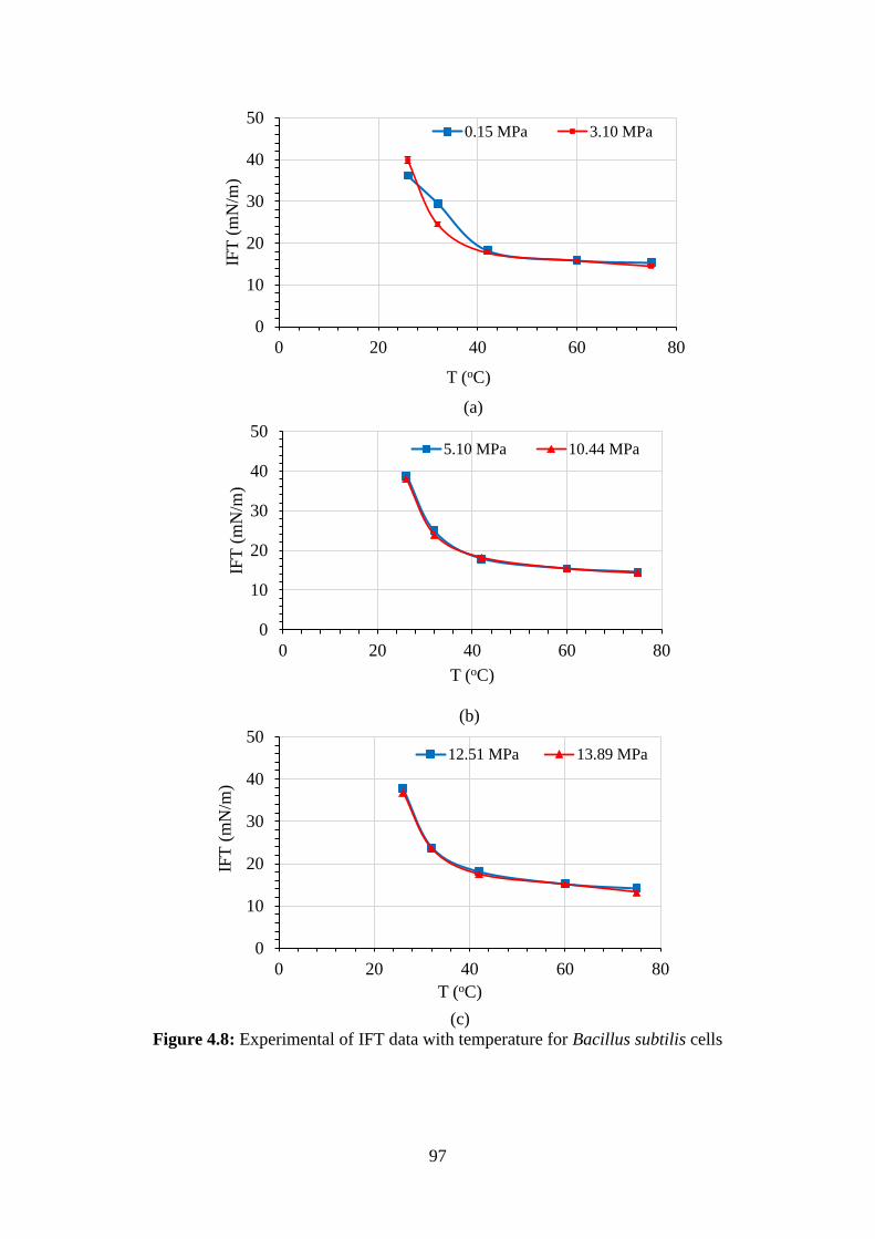
97

(a)

(b)

(c)

Figure 4.8: Experimental of IFT data with temperature for Bacillus subtilis cells

0

10

20

30

40

50

0 20 40 60 80

IFT

(m

N/m

)

T (oC)

0.15 MPa 3.10 MPa

0

10

20

30

40

50

0 20 40 60 80

IFT

(m

N/m

)

T (oC)

5.10 MPa 10.44 MPa

0

10

20

30

40

50

0 20 40 60 80

IFT

(m

N/m

)

T (oC)

12.51 MPa 13.89 MPa

98

Figure 4.9 is a plot of the variation of IFT with pressure for BS-1 cells. An increase in

pressure did not show any significant reduction in interfacial tension except at 3.10 MPa

(26oC and 32oC) where minimal increase and decrease of IFT was seen. This conforms to

conclusion made by Cai, Yang, & Guo, (1996), that IFT is weakly dependent on pressure.

Figure 4.9: Pressure effect on IFT for BS-1 cells

The Figure and data of a series of IFT trend with time obtained at three different temperature

and pressures is presented in Appendix E. Measurement at a given temperature and pressure

were always taken at intervals up to 3 minutes aging time, and often to 15 minutes. In

Appendix E-1, the biosurfactant capacity to reduce interfacial tension had negligible effect at

12.51 MPa (32oC) may be attributed to less microbial activity. The activity of the

biosurfactant was clearly seen in Appendix E-2 at 0.15 MPa (42oC) where the IFT reduced

from 18.23 mN/m to 17.73 mN/m and then increased across other selected pressures. This

reduction may well be due to the fact that there was a significant growth of microbial

population at that temperature and pressure. Recalling that Bacillus subtilis grow optimally

between temperatures of 37oC and 55oC. In Appendix E-3 there was a significant decrease in

IFT indicating a strong activity of the biosurfactant. However, after nine minutes of

incubation at 5.10 MPa (75oC) IFT increased for the remaining aging time.

0

5

10

15

20

25

30

35

40

45

0 5 10 15

IFT

/mN

.m-1

Pressure (MPa)

26 °C 32 °C 42 °C 60 °C 75 °C

99

4.3.1.2 Bacillus subtilis (BS-1) cell-free

The effect of BS-1 cell-free biosurfactant was adequately noticed in the reduction of IFT

investigated under thermophilic conditions. In Figure 4.10, the variation of IFT is seen to

decline in a similar trend that the isotherms overlap. In this analysis, IFT significantly

decreased from 47.06 mN/m to 10.94 mN/m (see also Appendix F) which was expected since

the effect of temperature dependence on IFT reduction is highly effective.

(a)

(b)

(c)

Figure 4.10: Temperature effect on IFT for BS-1 cell-free biosurfactant.

0

10

20

30

40

50

0 20 40 60 80

IFT

/mN

.m-1

T(oC)

0.15 MPa 3.10 MPa

0

20

40

60

0 20 40 60 80

IFT

(m

N/m

)

T (oC)

5.10 MPa 10.34 MPa

0

10

20

30

40

50

0 20 40 60 80

IFT

(m

N/m

)

T (oC)

12.51 MPa 13.89 MPa

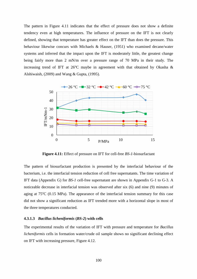
100

The pattern in Figure 4.11 indicates that the effect of pressure does not show a definite

tendency even at high temperatures. The influence of pressure on the IFT is not clearly

defined, showing that temperature has greater effect on the IFT than does the pressure. This

behaviour likewise concurs with Michaels & Hauser, (1951) who examined decane/water

systems and inferred that the impact upon the IFT is moderately little, the greatest change

being fairly more than 2 mN/m over a pressure range of 70 MPa in their study. The

increasing trend of IFT at 26oC maybe in agreement with that obtained by Okasha &

Alshiwaish, (2009) and Wang & Gupta, (1995).

Figure 4.11: Effect of pressure on IFT for cell-free BS-1-biosurfactant

The pattern of biosurfactant production is presented by the interfacial behaviour of the

bacterium, i.e. the interfacial tension reduction of cell free supernatants. The time variation of

IFT data (Appendix G) for BS-1 cell-free supernatant are shown in Appendix G-1 to G-3. A

noticeable decrease in interfacial tension was observed after six (6) and nine (9) minutes of

aging at 75oC (0.15 MPa). The appearance of the interfacial tension summary for this case

did not show a significant reduction as IFT trended more with a horizontal slope in most of

the three temperatures conducted.

4.3.1.3 Bacillus licheniformis (BS-2) with cells

The experimental results of the variation of IFT with pressure and temperature for Bacillus

licheniformis cells in formation water/crude oil sample shows no significant declining effect

on IFT with increasing pressure, Figure 4.12.

0

10

20

30

40

50

0 5 10 15

IFT

/mN

m-1

P/MPa

26 °C 32 °C 42 °C 60 °C 75 °C

101

Figure 4.12: Pressure effect on IFT for BS-2 biosurfactant cells

The analysis further revealed that under the same conditions of pressure, increasing

temperature and microbial activity, IFT decreases and is changing with a lower slope, Figure

4.13 (a). For IFT values of 13.10 mN/m (60oC) and 12.99 mN/m (75oC) respectively may

indicate that the concentration and activity of the biosurfactant (B. licheninformis cells)

molecule is approaching a stable value Appendix H. More interestingly as the interface ages,

it was observed in Figure 4.13 (b, c), that IFT showed a stable trend between 42oC and 60oC,

but further decreased down the slope. This may have resulted to abrupt changes in the

physical properties such as osmotic pressure and turbidity as the liquids (crude oil and

formation water) react with the biosurfactant concentration. It can therefore be inferred here

that the rate at which the osmotic pressure increases with microbial concentration turns out to

be unusually low, and the rate of increase of turbidity with concentration is highly improved,

which suggests that considerable association was taking place. Turbidity in the IFT cell will

look like the reaction in a broth culture which occur due to increase in the bacterial

population after growth.

0

5

10

15

20

25

30

35

40

45

0 5 10 15

IFT

/mN

.-1

Pressure (MPa)

26 °C 32 °C 42 °C 60 °C 75 °C

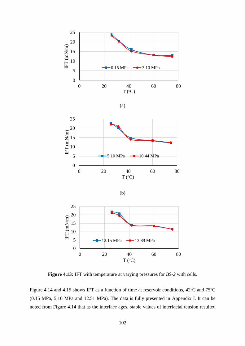
102

(a)

(b)

Figure 4.13: IFT with temperature at varying pressures for BS-2 with cells.

Figure 4.14 and 4.15 shows IFT as a function of time at reservoir conditions, 42oC and 75oC

(0.15 MPa, 5.10 MPa and 12.51 MPa). The data is fully presented in Appendix I. It can be

noted from Figure 4.14 that as the interface ages, stable values of interfacial tension resulted

0

5

10

15

20

25

0 20 40 60 80

IFT

(m

N/m

)

T (oC)

0.15 MPa 3.10 MPa

0

5

10

15

20

25

0 20 40 60 80

IFT

(m

N/m

)

T (oC)

5.10 MPa 10.44 MPa

0

5

10

15

20

25

0 20 40 60 80

IFT

(m

N/m

)

T (oC)

12.15 MPa 13.89 MPa

103

after 3 minutes for 0.15 MPa (42oC), while a gradual decline of interfacial tension value

occurred between the two other pressures. We found out that at a given temperature and

pressure, IFT didn’t show a significant decrease with time at 12.51 MPa (75oC), as IFT

initially was increasing (Figure 4.15). The uncommon decrease of IFT with time may be the

result of mutual solubility changes of the system with pressure, which may have resulted to

changes in the physical properties such as osmotic pressure and turbidity. However, no

literature was found to support this unusual effect.

Figure 4.14: IFT with time for BS-2 biosurfactant at 42oC

Figure 4.15: Variation of IFT with time for BS-2 biosurfactant at 75oC

4.3.1.4 Bacillus licheniformis (BS-2) cell-free

Cell-free biosurfactant of Bacillus licheniformis gave the greatest reduction values of IFT as,

also seen in the data generated in Appendix J. It was assumed that equilibrium between the

liquids was reached after five minutes of forming the oil film before the measurement were

taken to observe the effect of the biosurfactant concentration . This is in conformity with

10

12

14

16

18

0 5 10 15 20

IFT

(m

N/m

)

Time (Mins)

0.15 MPa 5.10 MPa 12.15 MPa

10

12

14

16

18

0 5 10 15 20

IFT

(m

N/m

)

Time (Mins)

0.15 MPa 5.10 MPa 12.15 MPa

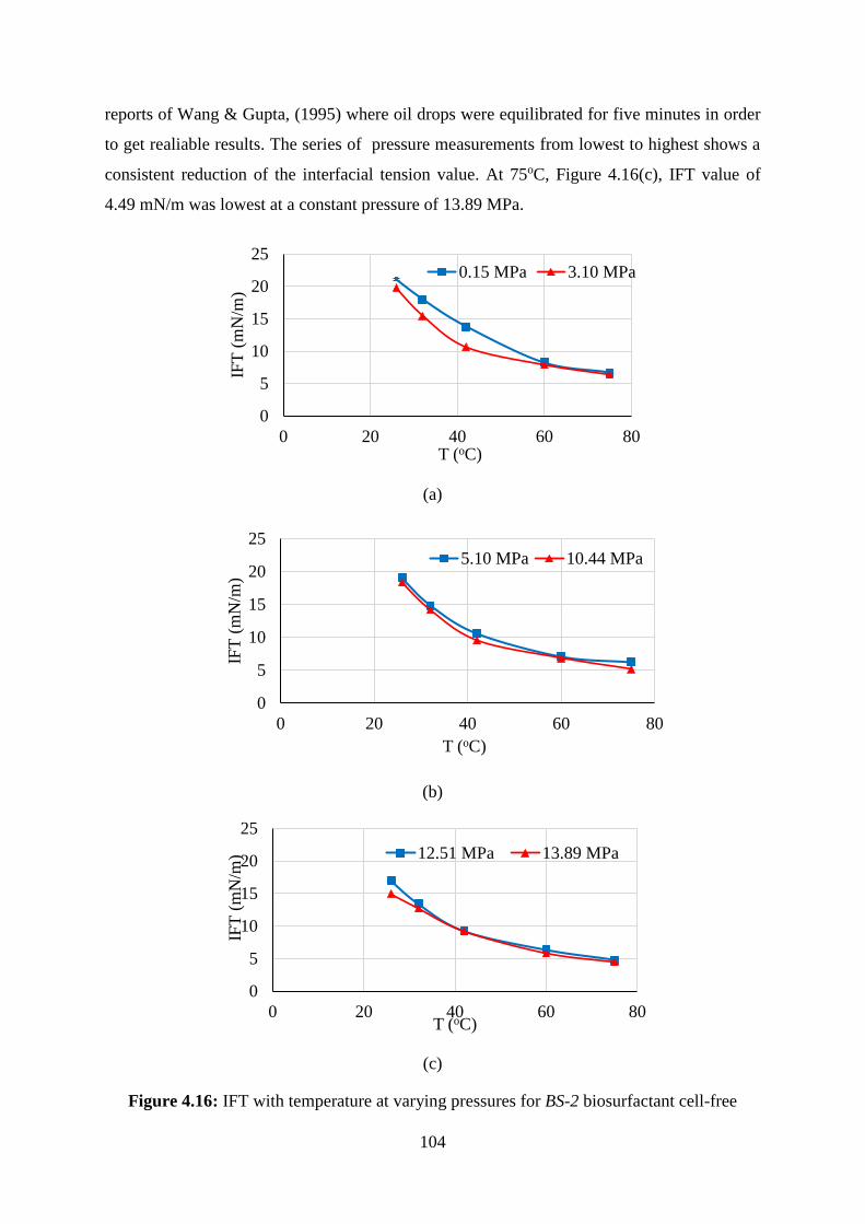
104

reports of Wang & Gupta, (1995) where oil drops were equilibrated for five minutes in order

to get realiable results. The series of pressure measurements from lowest to highest shows a

consistent reduction of the interfacial tension value. At 75oC, Figure 4.16(c), IFT value of

4.49 mN/m was lowest at a constant pressure of 13.89 MPa.

(a)

(b)

(c)

Figure 4.16: IFT with temperature at varying pressures for BS-2 biosurfactant cell-free

0

5

10

15

20

25

0 20 40 60 80

IFT

(m

N/m

)

T (oC)

0.15 MPa 3.10 MPa

0

5

10

15

20

25

0 20 40 60 80

IFT

(m

N/m

)

T (oC)

5.10 MPa 10.44 MPa

0

5

10

15

20

25

0 20 40 60 80

IFT

(m

N/m

)

T (oC)

12.51 MPa 13.89 MPa

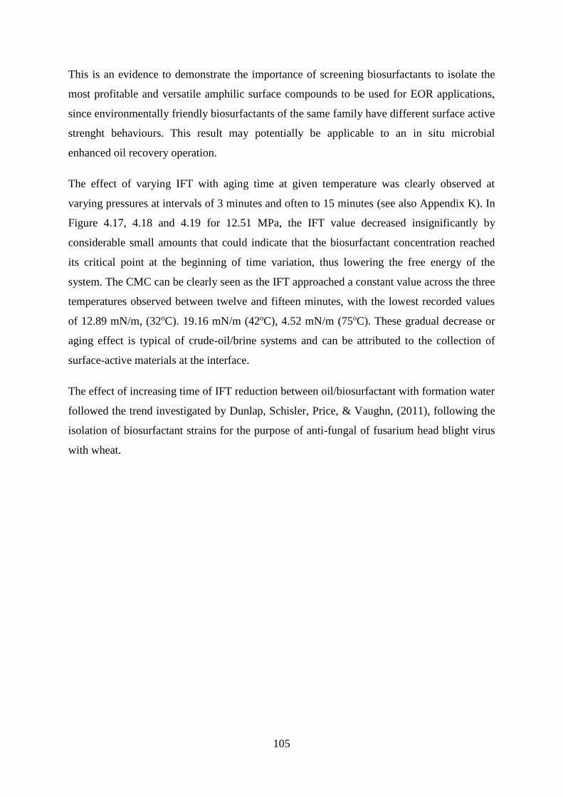
105

This is an evidence to demonstrate the importance of screening biosurfactants to isolate the

most profitable and versatile amphilic surface compounds to be used for EOR applications,

since environmentally friendly biosurfactants of the same family have different surface active

strenght behaviours. This result may potentially be applicable to an in situ microbial

enhanced oil recovery operation.

The effect of varying IFT with aging time at given temperature was clearly observed at

varying pressures at intervals of 3 minutes and often to 15 minutes (see also Appendix K). In

Figure 4.17, 4.18 and 4.19 for 12.51 MPa, the IFT value decreased insignificantly by

considerable small amounts that could indicate that the biosurfactant concentration reached

its critical point at the beginning of time variation, thus lowering the free energy of the

system. The CMC can be clearly seen as the IFT approached a constant value across the three

temperatures observed between twelve and fifteen minutes, with the lowest recorded values

of 12.89 mN/m, (32oC). 19.16 mN/m (42oC), 4.52 mN/m (75oC). These gradual decrease or

aging effect is typical of crude-oil/brine systems and can be attributed to the collection of

surface-active materials at the interface.

The effect of increasing time of IFT reduction between oil/biosurfactant with formation water

followed the trend investigated by Dunlap, Schisler, Price, & Vaughn, (2011), following the

isolation of biosurfactant strains for the purpose of anti-fungal of fusarium head blight virus

with wheat.

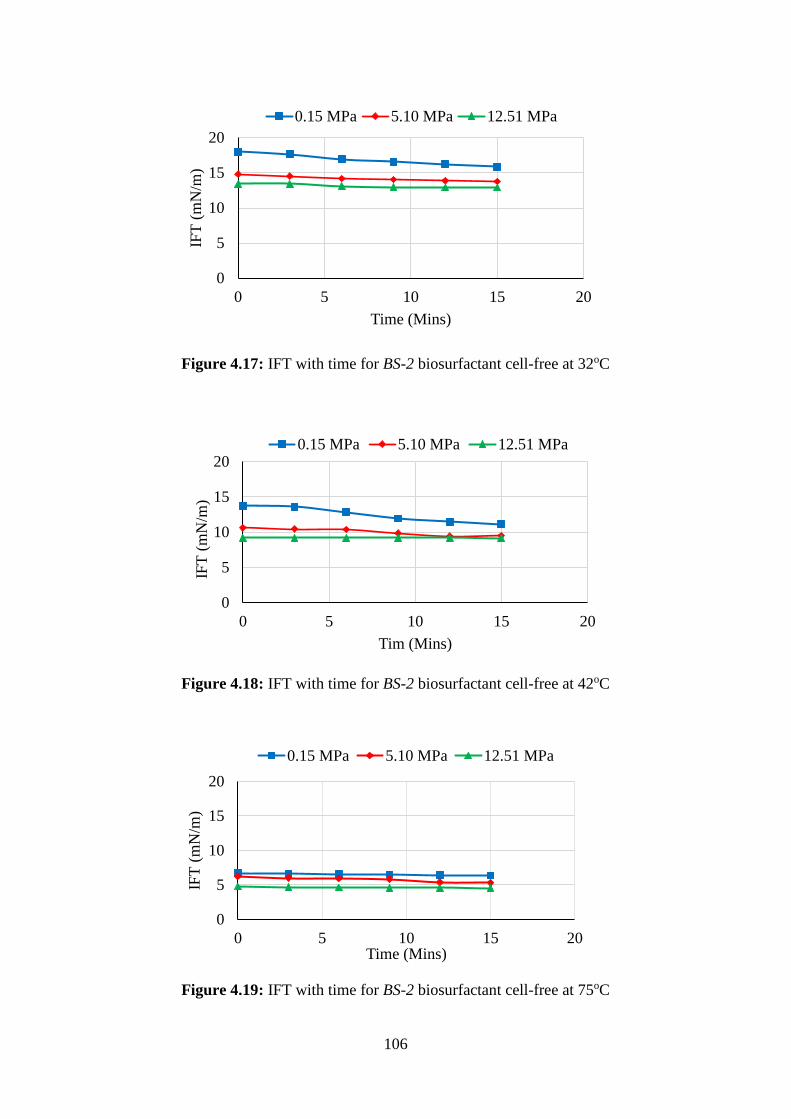
106

Figure 4.17: IFT with time for BS-2 biosurfactant cell-free at 32oC



0

5

10

15

20

0 5 10 15 20

IFT

(m

N/m

)

Time (Mins)

0.15 MPa 5.10 MPa 12.51 MPa

0

5

10

15

20

0 5 10 15 20

IFT

(m

N/m

)

Tim (Mins)

0.15 MPa 5.10 MPa 12.51 MPa

0

5

10

15

20

0 5 10 15 20

IFT

(m

N/m

)

Time (Mins)

0.15 MPa 5.10 MPa 12.51 MPa

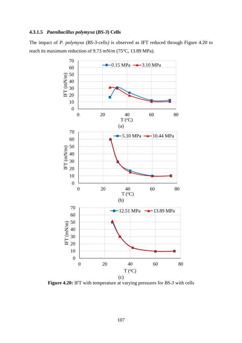
107

4.3.1.5 Paenibacillus polymyxa (BS-3) Cells

The impact of P. polymyxa (BS-3-cells) is observed as IFT reduced through Figure 4.20 to

reach its maximum reduction of 9.73 mN/m (75oC, 13.89 MPa).

(a)

(b)

(c)

Figure 4.20: IFT with temperature at varying pressures for BS-3 with cells

0

10

20

30

40

50

60

70

0 20 40 60 80

IFT

(m

N/m

)

T (oC)

0.15 MPa 3.10 MPa

0

10

20

30

40

50

60

70

0 20 40 60 80

IFT

(m

N/m

)

T (oC)

5.10 MPa 10.44 MPa

0

10

20

30

40

50

60

70

0 20 40 60 80

IFT

(m

N/m

)

T (oC)

12.51 MPa 13.89 MPa

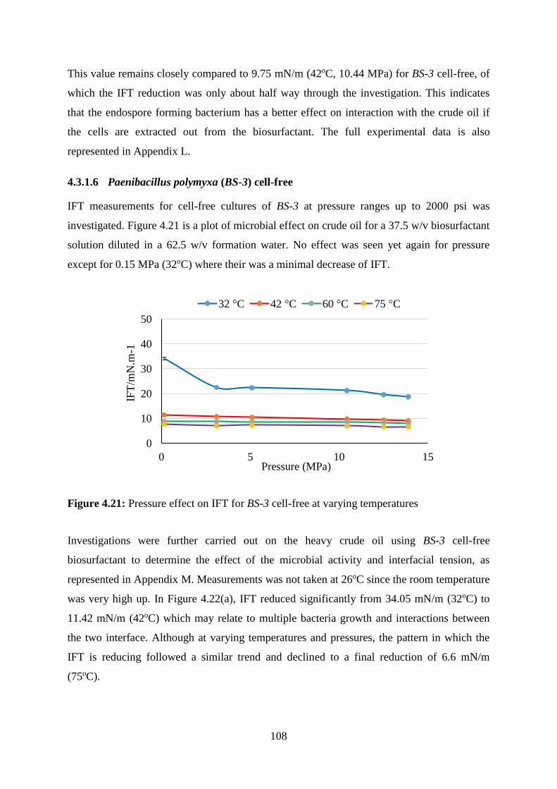
108

This value remains closely compared to 9.75 mN/m (42oC, 10.44 MPa) for BS-3 cell-free, of

which the IFT reduction was only about half way through the investigation. This indicates

that the endospore forming bacterium has a better effect on interaction with the crude oil if

the cells are extracted out from the biosurfactant. The full experimental data is also

represented in Appendix L.

4.3.1.6 Paenibacillus polymyxa (BS-3) cell-free

IFT measurements for cell-free cultures of BS-3 at pressure ranges up to 2000 psi was

investigated. Figure 4.21 is a plot of microbial effect on crude oil for a 37.5 w/v biosurfactant

solution diluted in a 62.5 w/v formation water. No effect was seen yet again for pressure

except for 0.15 MPa (32oC) where their was a minimal decrease of IFT.

Figure 4.21: Pressure effect on IFT for BS-3 cell-free at varying temperatures

Investigations were further carried out on the heavy crude oil using BS-3 cell-free

biosurfactant to determine the effect of the microbial activity and interfacial tension, as

represented in Appendix M. Measurements was not taken at 26oC since the room temperature

was very high up. In Figure 4.22(a), IFT reduced significantly from 34.05 mN/m (32oC) to

11.42 mN/m (42oC) which may relate to multiple bacteria growth and interactions between

the two interface. Although at varying temperatures and pressures, the pattern in which the

IFT is reducing followed a similar trend and declined to a final reduction of 6.6 mN/m

(75oC).

0 5 10 15

0

10

20

30

40

50

Pressure (MPa)

IFT

/mN

.m-1

32 °C 42 °C 60 °C 75 °C

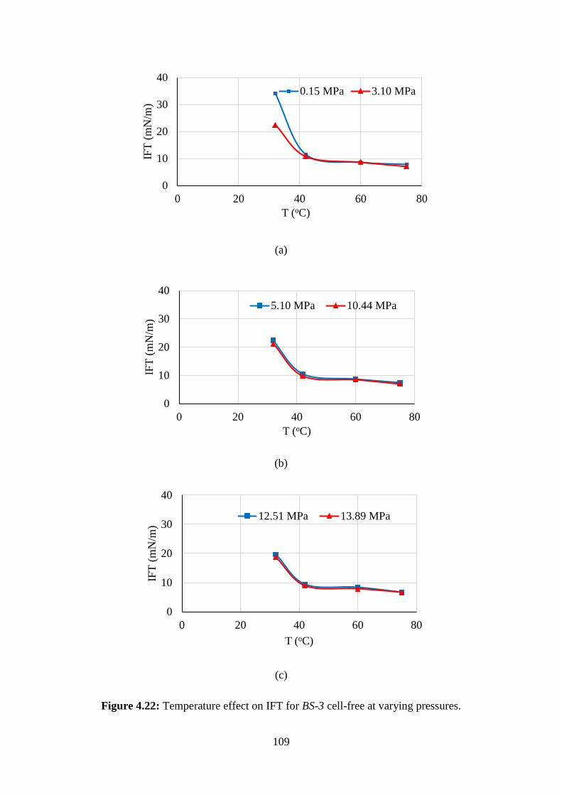
109

(a)

(b)

(c)

Figure 4.22: Temperature effect on IFT for BS-3 cell-free at varying pressures.

0

10

20

30

40

0 20 40 60 80

IFT

(m

N/m

)

T (oC)

0.15 MPa 3.10 MPa

0

10

20

30

40

0 20 40 60 80

IFT

(m

N/m

)

T (oC)

5.10 MPa 10.44 MPa

0

10

20

30

40

0 20 40 60 80

IFT

(m

N/m

)

T (oC)

12.51 MPa 13.89 MPa

110

The plot for IFT with time at constant pressure in 32oC and 42oC for BS-3 cell-free

supernatant is presented in Appendix N-1 and N-2. The lowest reduction recorded at 42oC

was 10.07 mN/m, and it was observed that this reduction was the same at 12 mins and 15

mins of the time measured. This reduction followed a similar pattern by (H. S. Al-Sulaimani

et al., 2010), where strain W19 gave a maximum IFT reduction to 3.28 mN/m in 16 hours of

incubation.

4.3.1.7 Comparison of IFT with temperature and time for BS-1, BS-2 and BS-3

Biosurfactants with Cells

In aqueous surfactant solutions, there is a large body of data on the surface and interfacial

tension which demonstrates that the structure of the surfactant molecule has a pronounced

capacity to reduce these tensions (Möbius, Miller, & Fainerman, 2001). However, this study

was not able to verify the biological structures of these produced biosurfactants, since it was

a costly process to undertake a mass spectrometry of the lipopeptide. I however assumed their

structures to be like that of surfactin, since they belong to the same family of lipopeptide.

Comparison of the cultured biosurfactants with cells in terms of IFT and contact angle

reduction, showed higher values when compared to interactions with cultured cell-free

biosurfactants at constant pressures as shown in Figure 4.23. Measurements of interfacial

tension reduction by these three biosurfactants with cells showed that Paenibacillus polymyxa

(BS-3) gave the greatest IFT reduction of 9.73 mN/m. This could be because BS-3 was

isolated from an oil field, which explains this interfacial activity. However, at the start of the

experiment, Appendix O, IFT can be seen to be constantly increasing, and may have resulted

due to a slow interaction of BS-3 cells with the oil, since further down, the effect was

significantly noticed.

The influence of pressure on the IFT is not clearly defined and did not indicate any

significant reduction in interfacial tension, showing that temperature has a greater effect on

the IFT than does the pressure. This behaviour likewise concurs with conclusion made by Cai

et al., (1996), that IFT is weakly dependent on pressure. Michaels and Hauser, (1951) who

examined decane/water systems and inferred that the impact upon the IFT is moderately

little, the greatest change being more than 2 mN/m over a pressure range of 70 MPa in their

report. However, the sharp increase of IFT at 26oC for cell-free BS-1, maybe in agreement

111

with results obtained by Wang and Gupta, (1995) and Okasha and Alshiwaish, (2009) when

IFT increased with pressure at constant temperature.

Further data are also shown in Appendix P that there was an insignificant reduction in IFT

with time for all three biosurfactants as the trend followed a reduction parallel to each other.

(a) At constant pressure of 0.15 MPa (b) At constant pressure of 3.10 MPa

(c) At constant pressure of 5.10 MPa (d) At constant pressure of 10.44 MPa

(e) At constant pressure of 12.51 MPa (f) At constant pressure of 13.89 MPa

Figure 4.23: Comparison of IFT with temperature for biosurfactants with cells

20 40 60 80

0

10

20

30

40

50

60

T (oC)

IFT

(m

N/m

)

BS 1 BS 2 BS 3

20 40 60 80

0

10

20

30

40

50

60

T (oC)IF

T (

mN

/m)

BS 1 BS 2 BS 3

20 40 60 80

0

10

20

30

40

50

60

T (oC)

IFT

(m

N/m

)

BS 1 BS 2 BS 3

20 40 60 80

0

10

20

30

40

50

60

T (oC)

IFT

(m

N/m

)

BS 1 BS 2 BS 3

20 40 60 80

0

10

20

30

40

50

60

T (oC)

IFT

(m

N/m

)

BS 1 BS 2 BS 3

20 40 60 80

0

10

20

30

40

50

60

T (oC)

IFT

(m

N/m

)

BS 1 BS 2 BS 3

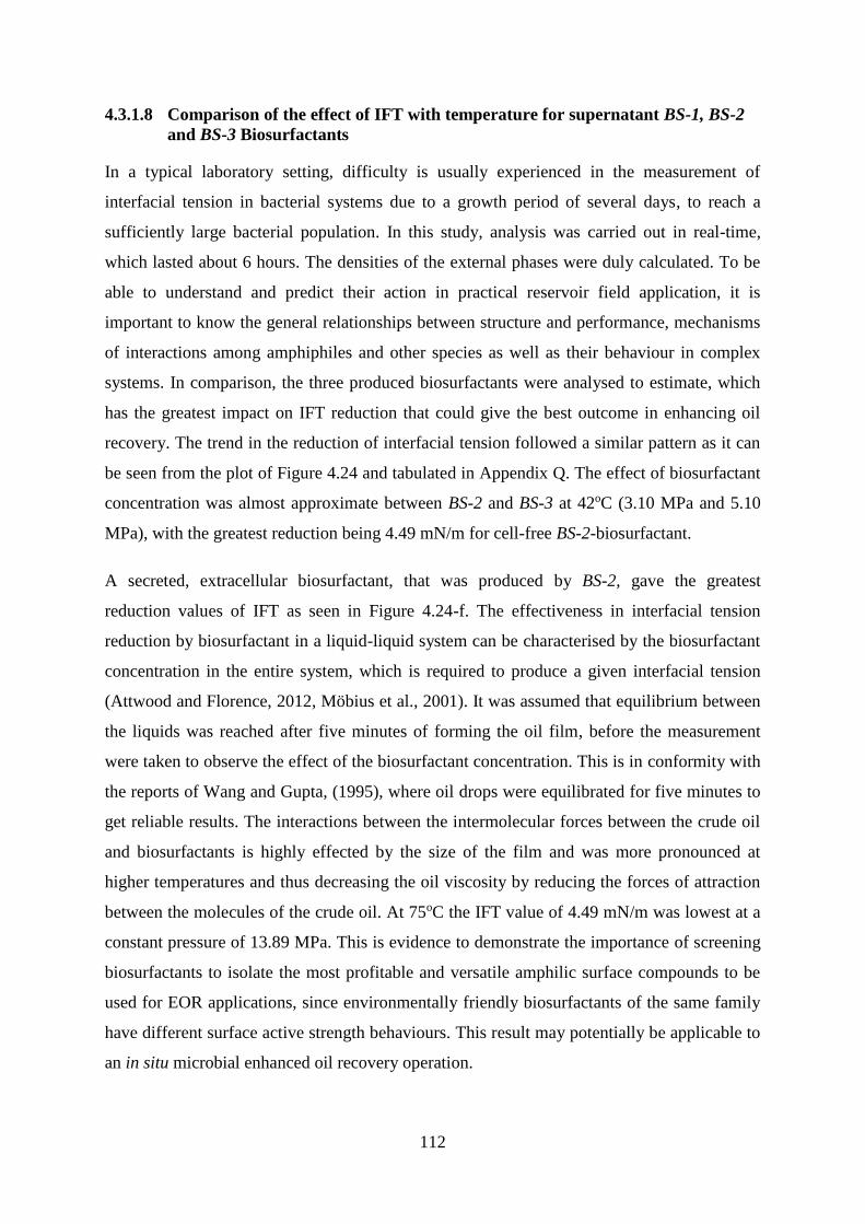
112

4.3.1.8 Comparison of the effect of IFT with temperature for supernatant BS-1, BS-2

and BS-3 Biosurfactants

In a typical laboratory setting, difficulty is usually experienced in the measurement of

interfacial tension in bacterial systems due to a growth period of several days, to reach a

sufficiently large bacterial population. In this study, analysis was carried out in real-time,

which lasted about 6 hours. The densities of the external phases were duly calculated. To be

able to understand and predict their action in practical reservoir field application, it is

important to know the general relationships between structure and performance, mechanisms

of interactions among amphiphiles and other species as well as their behaviour in complex

systems. In comparison, the three produced biosurfactants were analysed to estimate, which

has the greatest impact on IFT reduction that could give the best outcome in enhancing oil

recovery. The trend in the reduction of interfacial tension followed a similar pattern as it can

be seen from the plot of Figure 4.24 and tabulated in Appendix Q. The effect of biosurfactant

concentration was almost approximate between BS-2 and BS-3 at 42oC (3.10 MPa and 5.10

MPa), with the greatest reduction being 4.49 mN/m for cell-free BS-2-biosurfactant.

A secreted, extracellular biosurfactant, that was produced by BS-2, gave the greatest

reduction values of IFT as seen in Figure 4.24-f. The effectiveness in interfacial tension

reduction by biosurfactant in a liquid-liquid system can be characterised by the biosurfactant

concentration in the entire system, which is required to produce a given interfacial tension

(Attwood and Florence, 2012, Möbius et al., 2001). It was assumed that equilibrium between

the liquids was reached after five minutes of forming the oil film, before the measurement

were taken to observe the effect of the biosurfactant concentration. This is in conformity with

the reports of Wang and Gupta, (1995), where oil drops were equilibrated for five minutes to

get reliable results. The interactions between the intermolecular forces between the crude oil

and biosurfactants is highly effected by the size of the film and was more pronounced at

higher temperatures and thus decreasing the oil viscosity by reducing the forces of attraction

between the molecules of the crude oil. At 75oC the IFT value of 4.49 mN/m was lowest at a

constant pressure of 13.89 MPa. This is evidence to demonstrate the importance of screening

biosurfactants to isolate the most profitable and versatile amphilic surface compounds to be

used for EOR applications, since environmentally friendly biosurfactants of the same family

have different surface active strength behaviours. This result may potentially be applicable to

an in situ microbial enhanced oil recovery operation.

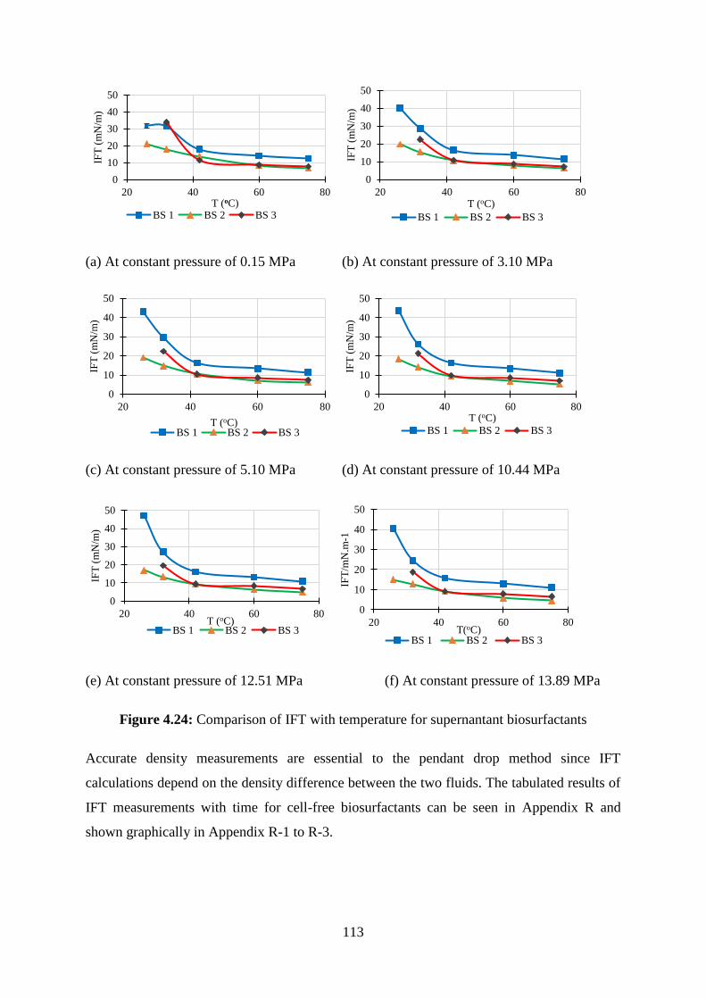
113

(a) At constant pressure of 0.15 MPa (b) At constant pressure of 3.10 MPa

(c) At constant pressure of 5.10 MPa (d) At constant pressure of 10.44 MPa

(e) At constant pressure of 12.51 MPa (f) At constant pressure of 13.89 MPa

Figure 4.24: Comparison of IFT with temperature for supernantant biosurfactants

Accurate density measurements are essential to the pendant drop method since IFT

calculations depend on the density difference between the two fluids. The tabulated results of

IFT measurements with time for cell-free biosurfactants can be seen in Appendix R and

shown graphically in Appendix R-1 to R-3.

0

10

20

30

40

50

20 40 60 80

IFT

(m

N/m

)

T (oC)BS 1 BS 2 BS 3

0

10

20

30

40

50

20 40 60 80

IFT

(m

N/m

)

T (oC)

BS 1 BS 2 BS 3

0

10

20

30

40

50

20 40 60 80

IFT

(m

N/m

)


0

10

20

30

40

50

20 40 60 80

IFT

(m

N/m

)

T (oC)

BS 1 BS 2 BS 3

0

10

20

30

40

50

20 40 60 80

IFT

(m

N/m

)


0

10

20

30

40

50

20 40 60 80

IFT

/mN

.m-1

T(oC)BS 1 BS 2 BS 3

114

The data displayed a time variation of 15 minutes at selected pressures. No meaningful

reduction of interfacial tension occurred except for BS-3 at 32oC (0.15 MPa) where a steep

decrease of IFT from 36.74 mN/m - 18.82 mN/m was observed. This pattern however,

indicated that IFT was weakly dependant on time, which could have resulted due to short

time variation in which the measurements were taken.

Contact Angle Measurements

Contact angle is the most acceptable measure of the natural wettability of a reservoir rock.

When a drop of liquid is placed on a surface immersed in another liquid, a contact angle is

formed which can range from 0o to 180o. A contact angle of 0o means total hydrophilicity,

which indicates completely water-wet, whereas and an angle of 180o means the surface is

totally hydrophobic, completely oil-wet. Wettability evaluation in the form of contact angle

estimation is a difficult type of measurement, since it is so sensitive to the surrounding

environment. In addition, Young’s equation (Eqn. 4.6) describes the sensitivity in the

measurement of a drop by considering the equilibrium between forces factors at the three-

phase-contact for oil/water/rock system.

𝜎𝑜𝑠 = 𝜎𝑤𝑠 + 𝜎𝑜𝑤. 𝑐𝑜𝑠𝜃 (4.6)

Where θ, is the contact angle at the oil/water/solid contact line, 𝜎𝑜𝑠, oil-solid (N/m), 𝜎𝑤𝑠, oil-

water (N/m), 𝜎𝑜𝑤, water-solid (N/m)

When the contact angle is greater than 90o, it is said to be oil-wet. If the angle is below 90o it

indicates water-wet surface, with a higher affinity for water than oil. If the surface shows

affinity for both phases, it is called intermediate-wet with an angle close to 90o. Since the

measurement techniques influence the value of contact angle, the angles measured by

different techniques may not be comparable. The generally accepted wetting classification is

given by (Anderson, 1986): 0o-75o, water-wet; 75o-115o, intermediate-wet; 115o-180o, oil-

wet. In this study, 95o-115o was defined as weakly intermediate-wet and 115o-135o was

defined as weakly oil-wet.

The results obtained from this study for the contact angle investigation was summarised and

presented with the lowest reductions for all the biosurfactant applied to the system. The

contact angle of the oil film reduced from 147.04o to 111.84o. Table 4.1, represents a

115

summary of this reductions which was recorded at different pressures and at elevated

temperature of 75oC.

Table 4.1: Greatest contact angle reduction of all produced biosurfactant

Parameters

Temperature

(oC)

Pressure

(MPa)

Contact

Angle (o)

Formation water 75 12.51 147.04

BS-1 Cells 75 13.89 135.86

BS-1 Cell-free 75 5.10 131.35

BS-2 Cells 75 10.44 125.11

BS-2 Cell-free 75 0.15 111.84

BS-3 Cells 75 12.51 133.36

BS-3 Cell-free 75 13.89 130.66

As the pressure increased, the contact angle became smaller and for most of the biosurfactant

applied to the system, the contact angle remained weakly oil-wet, mostly ranging between

125o to 136o. Although, the effect of BS-2 cell-free biosurfactant was significant enough to

reduce the contact angle to 111.84o, a weakly intermediate-wet state as seen in Figure 4.25.

However, none of the biosurfactants could reduce the contact angle enough to alter the

wettability of the oil film into a water-wet state. Although, the low salinity of the formation

water which influenced the preparation of the MSM used during the bacteria culture, could

have affected the outcome of the results. Thus, for each scenario investigated in this study,

the contact angle decreases as the temperature was increased, which means that the system

was greatly influenced at elevated temperature.

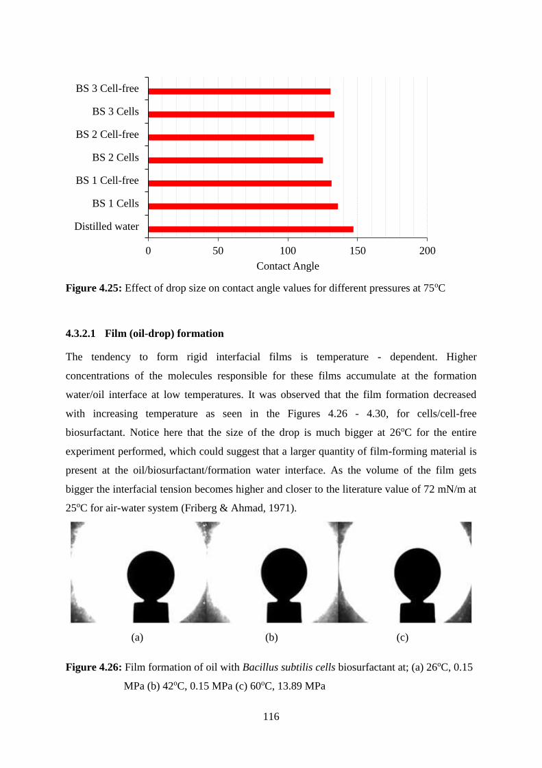
116

Figure 4.25: Effect of drop size on contact angle values for different pressures at 75oC

4.3.2.1 Film (oil-drop) formation

The tendency to form rigid interfacial films is temperature - dependent. Higher

concentrations of the molecules responsible for these films accumulate at the formation

water/oil interface at low temperatures. It was observed that the film formation decreased

with increasing temperature as seen in the Figures 4.26 - 4.30, for cells/cell-free

biosurfactant. Notice here that the size of the drop is much bigger at 26oC for the entire

experiment performed, which could suggest that a larger quantity of film-forming material is

present at the oil/biosurfactant/formation water interface. As the volume of the film gets

bigger the interfacial tension becomes higher and closer to the literature value of 72 mN/m at

25oC for air-water system (Friberg & Ahmad, 1971).

(a) (b) (c)

Figure 4.26: Film formation of oil with Bacillus subtilis cells biosurfactant at; (a) 26oC, 0.15

MPa (b) 42oC, 0.15 MPa (c) 60oC, 13.89 MPa

0 50 100 150 200

Distilled water

BS 1 Cells

BS 1 Cell-free

BS 2 Cells

BS 2 Cell-free

BS 3 Cells

BS 3 Cell-free

Contact Angle

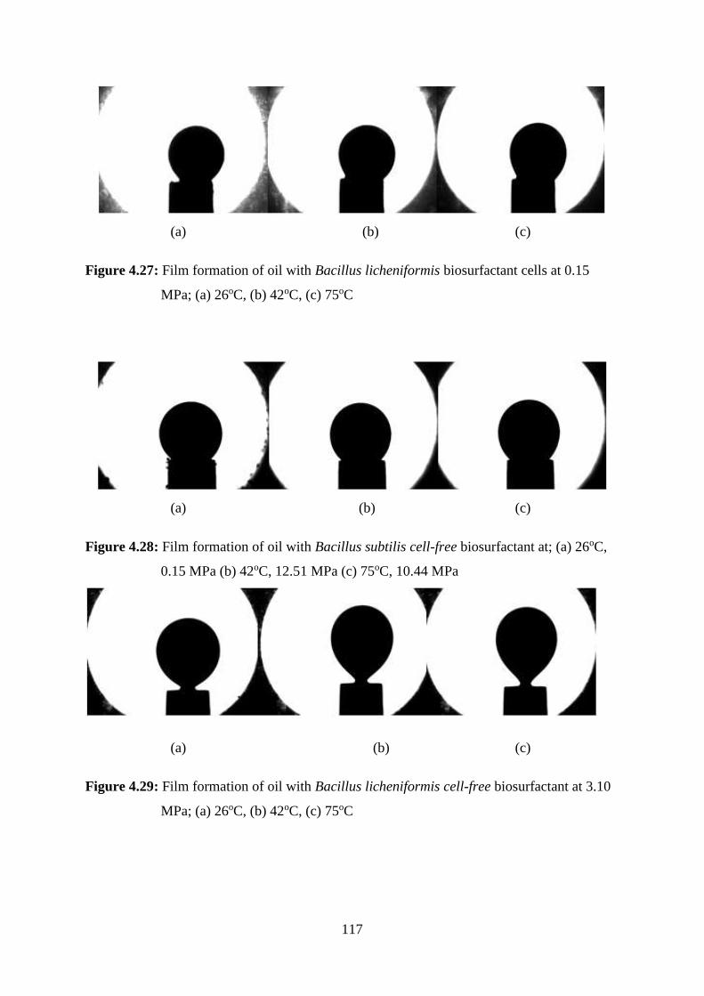
117

(a) (b) (c)

Figure 4.27: Film formation of oil with Bacillus licheniformis biosurfactant cells at 0.15

MPa; (a) 26oC, (b) 42oC, (c) 75oC

(a) (b) (c)

Figure 4.28: Film formation of oil with Bacillus subtilis cell-free biosurfactant at; (a) 26oC,

0.15 MPa (b) 42oC, 12.51 MPa (c) 75oC, 10.44 MPa

(a) (b) (c)

Figure 4.29: Film formation of oil with Bacillus licheniformis cell-free biosurfactant at 3.10

MPa; (a) 26oC, (b) 42oC, (c) 75oC

118

(a) (b) (c)

Figure 4.30: Film formation of oil with paenibacillus polymyxa cell-free biosurfactant at

10.44 MPa (a) 32oC, (b) 42oC, (c) 75oC

The ability to form interfacial films, as well as the type of film, has been shown to be closely

related to the amount of polar compounds (i.e. asphaltenes and resins) in the crude oil as well

as brine pH (Hasiba & Jessen, 1968; Strassner, 1968). In this study, the impact of pH on

interfacial tension was not examined. The transition of a rigid film into a liquid expanded

film may explain the reduction of film size with temperature Davies & Rideal, (1963). In all

the oil film framed in this study, the shape was spherical with a clearly formed neck, except

for BS-2 cells and BS-3 cell-free that did not form a clear neck. Subsequently, measures were

taking into consideration, by adjusting the horizontal cross-hair line to the point of

convergence before taking the IFT measurements.

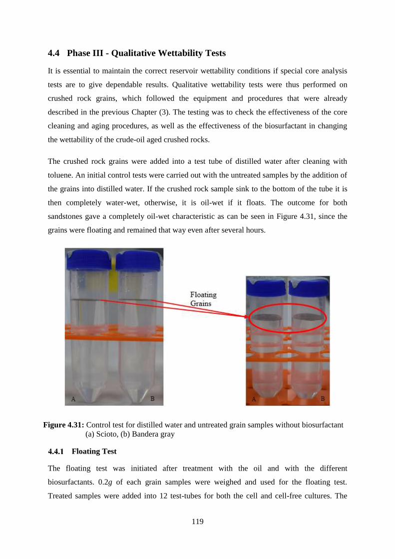
119

4.4 Phase III - Qualitative Wettability Tests

It is essential to maintain the correct reservoir wettability conditions if special core analysis

tests are to give dependable results. Qualitative wettability tests were thus performed on

crushed rock grains, which followed the equipment and procedures that were already

described in the previous Chapter (3). The testing was to check the effectiveness of the core

cleaning and aging procedures, as well as the effectiveness of the biosurfactant in changing

the wettability of the crude-oil aged crushed rocks.

The crushed rock grains were added into a test tube of distilled water after cleaning with

toluene. An initial control tests were carried out with the untreated samples by the addition of

the grains into distilled water. If the crushed rock sample sink to the bottom of the tube it is

then completely water-wet, otherwise, it is oil-wet if it floats. The outcome for both

sandstones gave a completely oil-wet characteristic as can be seen in Figure 4.31, since the

grains were floating and remained that way even after several hours.

Figure 4.31: Control test for distilled water and untreated grain samples without biosurfactant

(a) Scioto, (b) Bandera gray

Floating Test

The floating test was initiated after treatment with the oil and with the different

biosurfactants. 0.2g of each grain samples were weighed and used for the floating test.

Treated samples were added into 12 test-tubes for both the cell and cell-free cultures. The

120

impressive performance of the effect of these biosurfactants was observed as the samples

were added into distilled water. Interestingly most of the outcome gave a positive effect in

altering the degree of wettability as can be seen in Figure 4.32 to 4.35. These results can be

compared to the floatation experiment conducted by Wu et al., (2006), where different

surfactants and naphthenic acids, treated with calcite powder, provided information about the

mechanisms responsible for the reversal to a water-wet state. The polar compounds in resins

and asphaltenes both combine hydrophilic and hydrophobic characteristics. Most of the

grains, treated with the biosurfactants, showed alteration in wettability from hydrophobic to a

slightly intermediate wet, rather than to a water-wet state, throughout the pore system for this

test. A summary of the results is presented in Table 4.2.

Figure 4.32: Distilled water and treated scioto grain sample in biosurfactant with cells

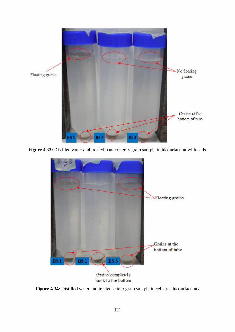
121

Figure 4.33: Distilled water and treated bandera gray grain sample in biosurfactant with cells

Figure 4.34: Distilled water and treated scioto grain sample in cell-free biosurfactants

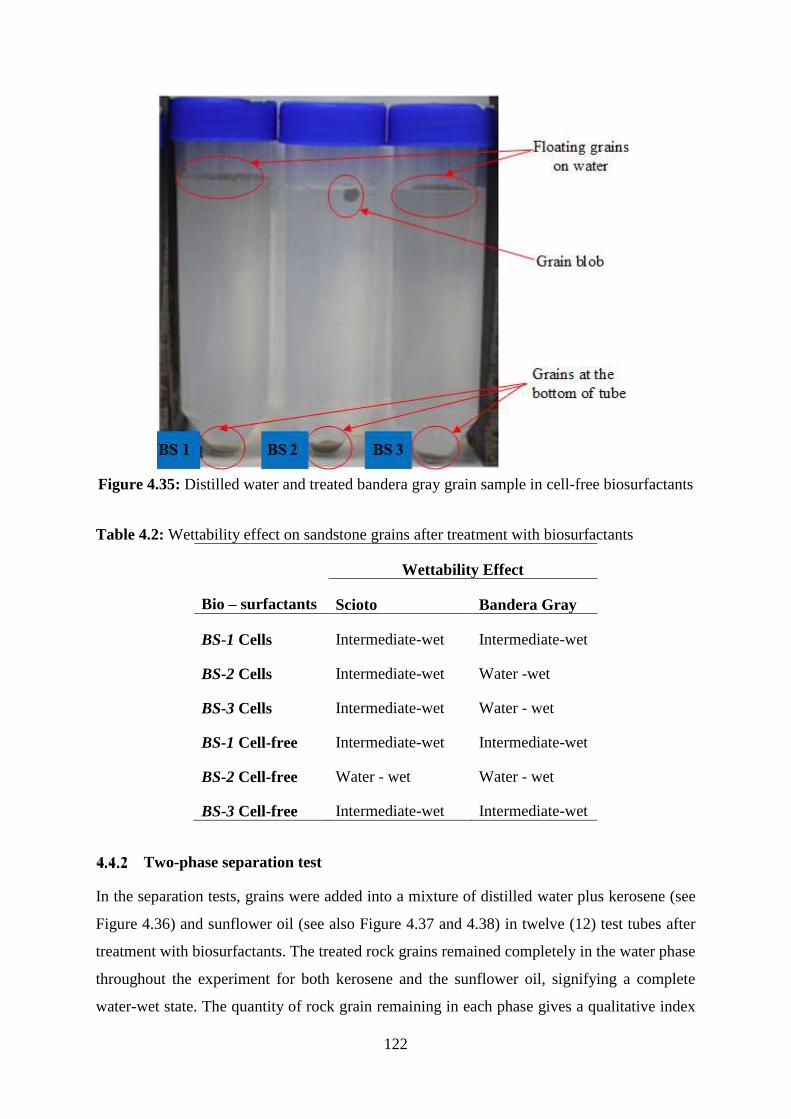
122

Figure 4.35: Distilled water and treated bandera gray grain sample in cell-free biosurfactants

Table 4.2: Wettability effect on sandstone grains after treatment with biosurfactants

Bio – surfactants

Wettability Effect

Scioto Bandera Gray

BS-1 Cells Intermediate-wet Intermediate-wet

BS-2 Cells Intermediate-wet Water -wet

BS-3 Cells Intermediate-wet Water - wet

BS-1 Cell-free Intermediate-wet Intermediate-wet

BS-2 Cell-free Water - wet Water - wet

BS-3 Cell-free Intermediate-wet Intermediate-wet

Two-phase separation test

In the separation tests, grains were added into a mixture of distilled water plus kerosene (see

Figure 4.36) and sunflower oil (see also Figure 4.37 and 4.38) in twelve (12) test tubes after

treatment with biosurfactants. The treated rock grains remained completely in the water phase

throughout the experiment for both kerosene and the sunflower oil, signifying a complete

water-wet state. The quantity of rock grain remaining in each phase gives a qualitative index

123

of its wettability, and according to (Somasundaran & Zhang, 2006), if the grains remain in

the oil phase, it is strongly oil wet, otherwise it is water wet.

Figure 4.36: Distilled water with kerosene plus treated grain samples in biosurfactants for

both cells and cell-free

124

Figure 4.37: Distilled water with sunflower plus treated grain sample in biosurfactant with

cells

Figure 4.38: Distilled water with sunflower plus treated grain sample in cell-free

biosurfactants.

125

Most sandstone reservoirs in the Niger Delta are not strongly water-wet, but are recognised

generally to exhibit a largely intermediate to slightly oil-wetting behaviour (McPhee, Reed,

& Zubizarreta, 2015). The wettability for Scioto and Bandera Gray, treated with these

biosurfactants, displayed an alteration in wettability from hydrophilic to hydrophobic,

characterised by the grains completely remaining in the aqueous phase. The crude oil utilised,

while preparing the grains, showed that it is a poor solvent for the biosurfactants, thus having

a greater propensity to change wettability (Al-Maamari & Buckley, 2003).

126

4.5 Phase - IV: Core flooding

The bio-flooding trials were conducted with a specific focus of investigating the effect of

biosurfactant injection on unsteady state flow behaviour of rock-fluids systems in changing

the wettability of the rock grain to further enhance oil recovery. These experiments were run

on a selected sandstone sample as described in Chapter-3, having same porosity and

permeability. All experiments were carried out using the core-flooding tests described

according to the procedures that were outlined in the previous Chapter (3).

One of the main objectives of this investigation was also to produce biosurfactant that can

ultimately improve oil recovery when compared with the conventional water flood. In order

to achieve this goal, the produced biosurfactant that gave the best outcome, (BS-2

supernatant), from the results obtained in IFT (Phase-II) and wettability experiments (Phase-

III) was selected. Also, the parameters needed to be established were, flowrate and pore

volume. This was necessitated to serve as a control for the initial conditions that will give an

ultimate recovery. Hence, 15 sets of core-flooding trials were conducted at different

repeatability runs, at flow rates of 0.75 ml/min, 0.5 ml/min and 0.25 ml/min, out of which 3

trials generated acceptable results which formed the basis of these series of experiments.

These different flow rates were ideal to obtain the optimum flowrate that gives the best

recovery prior to the injection of the biosurfactant. The best recovery was recorded at a flow

rate of 0.25 ml/min, with a breakthrough time of 246 minutes as shown in Figure 4.39.

During each of the injection cycle (preliminary and actual runs), on the average, about 13

pore volumes of biosurfactant/distilled water were injected into the core sample before

reaching stabilised conditions i.e. the displaced phase was no longer produced and reaching a

stable pressure drop across the sample.

In Figure 4.40, the performance of BS-2- supernatant flooding showed a significant amount

of oil was produced at a reduced breakthrough time with decrease in pore volume (PV)

compared to the water flooding, leading to a higher recovery rate.

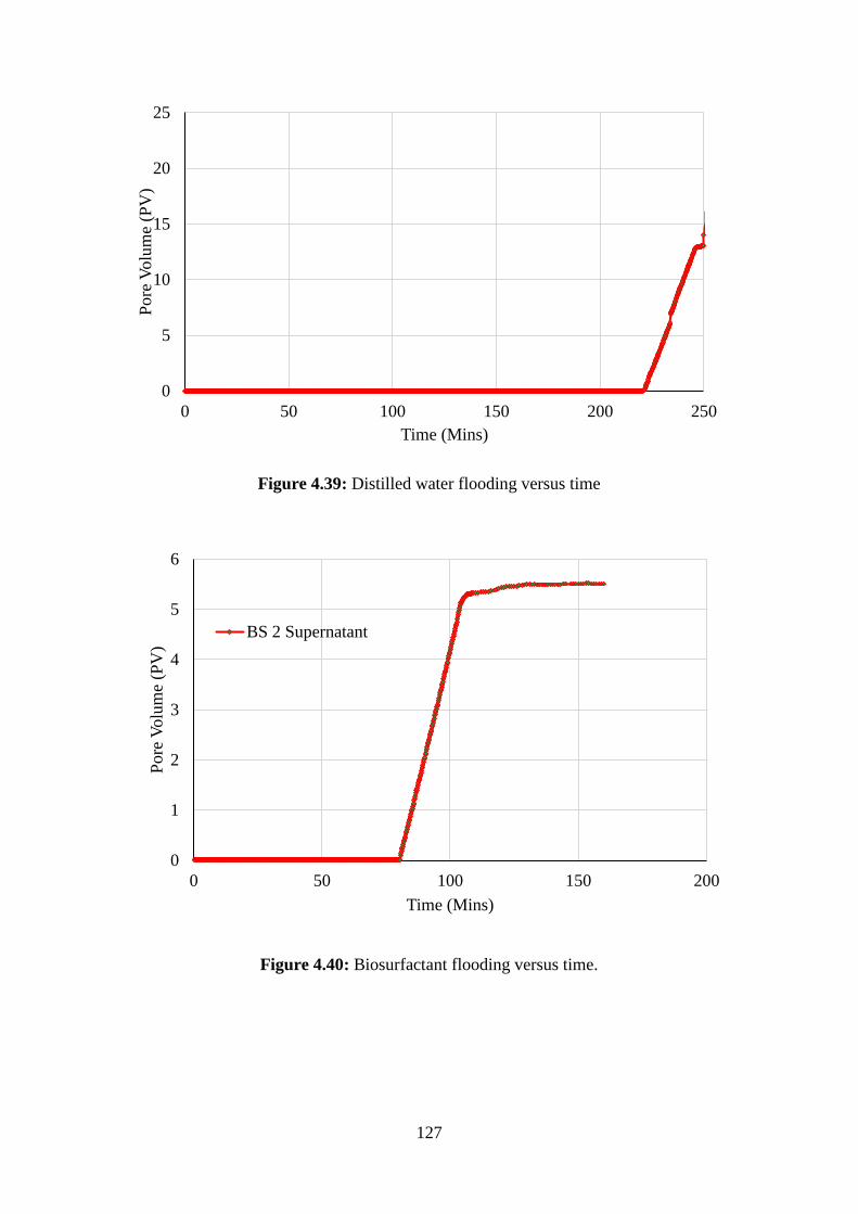
127

Figure 4.39: Distilled water flooding versus time

Figure 4.40: Biosurfactant flooding versus time.

0

5

10

15

20

25

0 50 100 150 200 250

Pore

Volu

me

(PV

)

Time (Mins)

0

1

2

3

4

5

6

0 50 100 150 200

Pore

Volu

me

(PV

)

Time (Mins)

BS 2 Supernatant

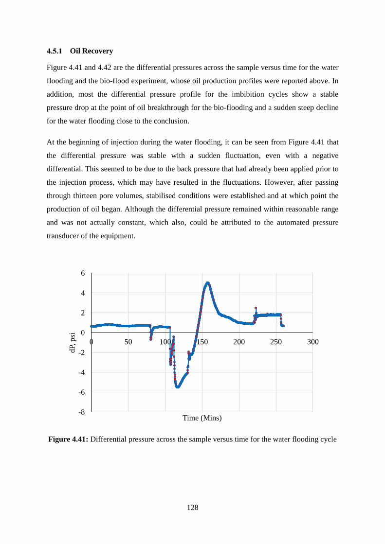
128

Oil Recovery

Figure 4.41 and 4.42 are the differential pressures across the sample versus time for the water

flooding and the bio-flood experiment, whose oil production profiles were reported above. In

addition, most the differential pressure profile for the imbibition cycles show a stable

pressure drop at the point of oil breakthrough for the bio-flooding and a sudden steep decline

for the water flooding close to the conclusion.

At the beginning of injection during the water flooding, it can be seen from Figure 4.41 that

the differential pressure was stable with a sudden fluctuation, even with a negative

differential. This seemed to be due to the back pressure that had already been applied prior to

the injection process, which may have resulted in the fluctuations. However, after passing

through thirteen pore volumes, stabilised conditions were established and at which point the

production of oil began. Although the differential pressure remained within reasonable range

and was not actually constant, which also, could be attributed to the automated pressure

transducer of the equipment.

Figure 4.41: Differential pressure across the sample versus time for the water flooding cycle

-8

-6

-4

-2

0

2

4

6

0 50 100 150 200 250 300

dP,

psi

Time (Mins)

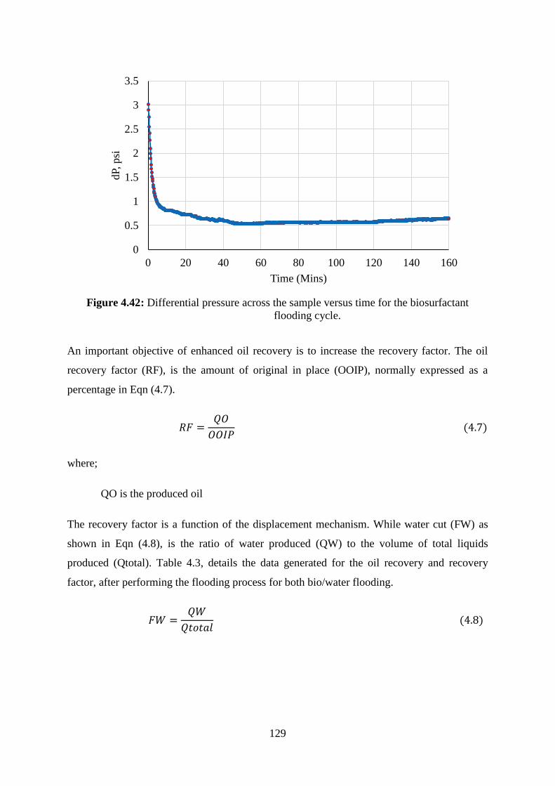
129

Figure 4.42: Differential pressure across the sample versus time for the biosurfactant

flooding cycle.

An important objective of enhanced oil recovery is to increase the recovery factor. The oil

recovery factor (RF), is the amount of original in place (OOIP), normally expressed as a

percentage in Eqn (4.7).

𝑅𝐹 =𝑄𝑂

𝑂𝑂𝐼𝑃 (4.7)

where;

QO is the produced oil

The recovery factor is a function of the displacement mechanism. While water cut (FW) as

shown in Eqn (4.8), is the ratio of water produced (QW) to the volume of total liquids

produced (Qtotal). Table 4.3, details the data generated for the oil recovery and recovery

factor, after performing the flooding process for both bio/water flooding.

𝐹𝑊 =𝑄𝑊

𝑄𝑡𝑜𝑡𝑎𝑙 (4.8)

0

0.5

1

1.5

2

2.5

3

3.5

0 20 40 60 80 100 120 140 160

dP,

psi

Time (Mins)

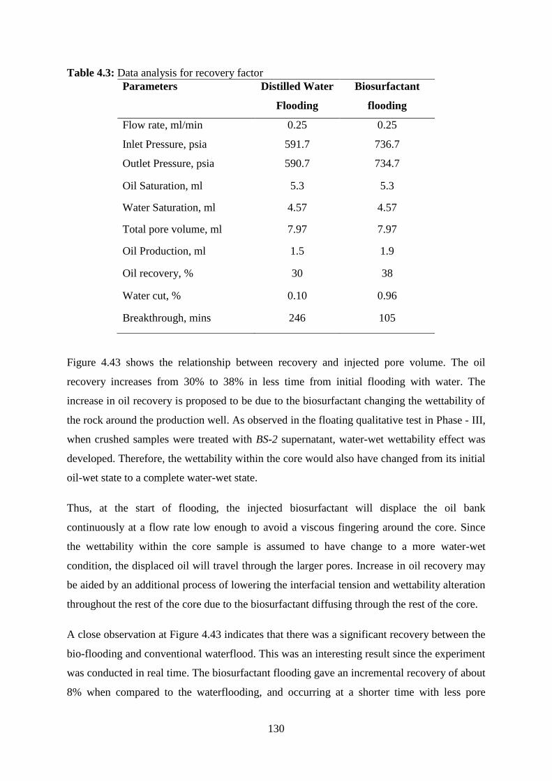
130

Table 4.3: Data analysis for recovery factor

Parameters Distilled Water

Flooding

Biosurfactant

flooding

Flow rate, ml/min 0.25 0.25

Inlet Pressure, psia 591.7 736.7

Outlet Pressure, psia 590.7 734.7

Oil Saturation, ml 5.3 5.3

Water Saturation, ml 4.57 4.57

Total pore volume, ml 7.97 7.97

Oil Production, ml 1.5 1.9

Oil recovery, % 30 38

Water cut, % 0.10 0.96

Breakthrough, mins 246 105

Figure 4.43 shows the relationship between recovery and injected pore volume. The oil

recovery increases from 30% to 38% in less time from initial flooding with water. The

increase in oil recovery is proposed to be due to the biosurfactant changing the wettability of

the rock around the production well. As observed in the floating qualitative test in Phase - III,

when crushed samples were treated with BS-2 supernatant, water-wet wettability effect was

developed. Therefore, the wettability within the core would also have changed from its initial

oil-wet state to a complete water-wet state.

Thus, at the start of flooding, the injected biosurfactant will displace the oil bank

continuously at a flow rate low enough to avoid a viscous fingering around the core. Since

the wettability within the core sample is assumed to have change to a more water-wet

condition, the displaced oil will travel through the larger pores. Increase in oil recovery may

be aided by an additional process of lowering the interfacial tension and wettability alteration

throughout the rest of the core due to the biosurfactant diffusing through the rest of the core.

A close observation at Figure 4.43 indicates that there was a significant recovery between the

bio-flooding and conventional waterflood. This was an interesting result since the experiment

was conducted in real time. The biosurfactant flooding gave an incremental recovery of about

8% when compared to the waterflooding, and occurring at a shorter time with less pore

131

volume. This indicates that the biosurfactant was effective in real time, and could be

attributed to its concentration and rich nutrient present, which will allow for the bacterial

growth and diffusion through the rest of the core. A very important observation made by

analysing the recovery trends is that the longer the saturation period is, the more time

available for the biosurfactant to redistribute in the core, and therefore more volume of oil

that will be produced.

Figure 4.43: Oil recovery curves with injected pore volumes

Al-Sulaimani et al., 2012 reported that biosurfactant had a potential for MEOR technology

because it yielded a total production of 23% of residual oil when treated with 0.25% (w/v)

biosurfactant. In this study, a total of 38% of residual oil was recovered when injected with

pure biosurfactant (BS-2) of 174.17 ml/L (w/v). In both cases, the biosurfactant used for the

core flooding were produced from a B. subtilis strain, W19 and BS-2 respectively. The core

flood experiments were also conducted at 60oC, to mimic the average reservoir temperature

of the field of interest. Oil production however, increased to 30% when injected with pure

chemical surfactant (Al-Sulaimani et al., 2012). Figure 4.44 presents a summary of these core

flooding results.

0

5

10

15

20

25

30

35

40

0 2 4 6 8 10 12 14

Rec

over

y (

%O

OIP

)

Pore Volume

Bioflooding

Water flooding

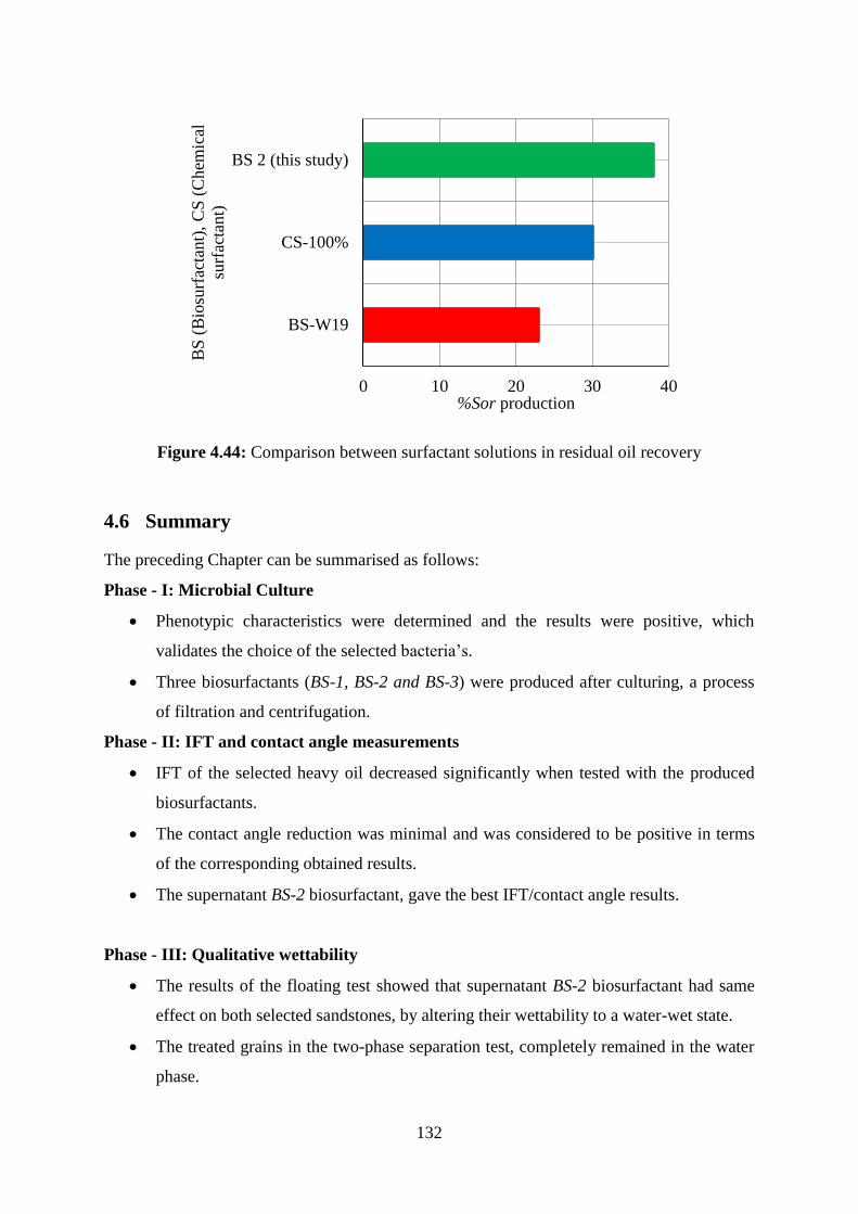
132

Figure 4.44: Comparison between surfactant solutions in residual oil recovery

4.6 Summary

The preceding Chapter can be summarised as follows:

Phase - I: Microbial Culture

Phenotypic characteristics were determined and the results were positive, which

validates the choice of the selected bacteria’s.

Three biosurfactants (BS-1, BS-2 and BS-3) were produced after culturing, a process

of filtration and centrifugation.

Phase - II: IFT and contact angle measurements

IFT of the selected heavy oil decreased significantly when tested with the produced

biosurfactants.

The contact angle reduction was minimal and was considered to be positive in terms

of the corresponding obtained results.

The supernatant BS-2 biosurfactant, gave the best IFT/contact angle results.

Phase - III: Qualitative wettability

The results of the floating test showed that supernatant BS-2 biosurfactant had same

effect on both selected sandstones, by altering their wettability to a water-wet state.

The treated grains in the two-phase separation test, completely remained in the water

phase.

0 10 20 30 40

BS-W19

CS-100%

BS 2 (this study)

%Sor production

BS

(B

iosu

rfac

tant)

, C

S (

Chem

ical

surf

acta

nt)

133

Phase – IV: Core Flooding

After flooding bandera gray with supernatant BS-2 biosurfactant, 38% of the residual

oil was recovered, which was a better outcome when compared with water flooding in

the same core system.

The next chapter will discuss the environmental risk assessment of the microbes selected to

produce the biosurfactants in this study.

134

Chapter 5

5 Risk Assessment in Utilising Biosurfactant produced from the Bacillus

Genus

5.1 Introduction

The environment is a broad concept that describes our biophysical surroundings. It includes

air, water, land and living organisms such as plants and wild life. Environmental risk

assessment is a scientific process that identifies and evaluates treats to the environment in

particular to living organism, habitats and ecosystems (Raz & Hillson, 2005). The causes of

environmental treats are diverse, some are natural, for example earthquake or volcanic

eruptions, whilst others might be as a result of human activities such as industrialization and

urbanisation. For instance, air pollution, toxic chemicals in food and water and sanitation. In

the petroleum industry, individual companies are responsible for carrying out risk assessment

for chemicals utilised during a recovery process that do not follow the natural production

process. This is because the use of these products may pose a risk to the environment.

This study evaluates the risk assessment in the following generalised areas to include, human

risk assessment and ecological risk assessment. The purpose of this assessment is to access

the seriousness and the likelihood of harm to the environment, which might arise following a

specific activity such as, inadequate controlled environment during bacteria culture and non-

treatment of wastewater. These assessments follow several stages as presented in Figure 5.1

beginning with the problem formulation. This is the first critical step because it defines the

scope of the environment risk assessment, by specifying what needs to be protected from

harm and by identifying potential harmful effects. This is then followed by a hazard and

exposure characterisation. In hazard characterisation, potential hazards and the seriousness of

potential harm are examined, while the exposure characterisation considers the likelihood and

the level of exposure to the hazards and thus how likely is it that harm will occur. The final

step involves the characterisation of risk. Here the seriousness and the likelihood of harm are

combined to estimate the level of risk. In some cases, the environmental risk assessment also

includes risk mitigation measure, such measures aim to reduce and identify risk to an

acceptable level or level of no concern (AIRMIC, 2002). This risk assessment is carried out

to ensure that the produced biosurfactant in Chapter-3, if used in an actual field in-situ

operation, do not cause an unacceptable harm to the environment.

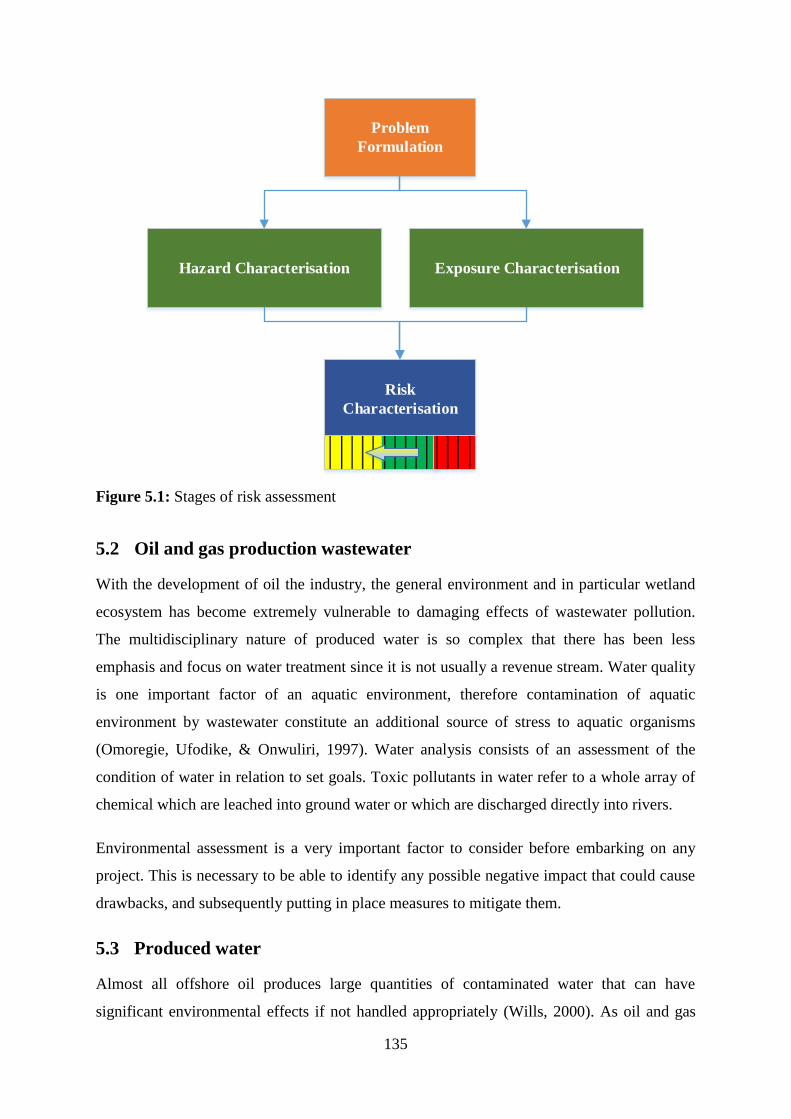
135

Hazard Characterisation Exposure Characterisation

Problem

Formulation

Risk

Characterisation

Figure 5.1: Stages of risk assessment

5.2 Oil and gas production wastewater

With the development of oil the industry, the general environment and in particular wetland

ecosystem has become extremely vulnerable to damaging effects of wastewater pollution.

The multidisciplinary nature of produced water is so complex that there has been less

emphasis and focus on water treatment since it is not usually a revenue stream. Water quality

is one important factor of an aquatic environment, therefore contamination of aquatic

environment by wastewater constitute an additional source of stress to aquatic organisms

(Omoregie, Ufodike, & Onwuliri, 1997). Water analysis consists of an assessment of the

condition of water in relation to set goals. Toxic pollutants in water refer to a whole array of

chemical which are leached into ground water or which are discharged directly into rivers.

Environmental assessment is a very important factor to consider before embarking on any

project. This is necessary to be able to identify any possible negative impact that could cause

drawbacks, and subsequently putting in place measures to mitigate them.

5.3 Produced water

Almost all offshore oil produces large quantities of contaminated water that can have

significant environmental effects if not handled appropriately (Wills, 2000). As oil and gas

136

production proceed, formation water eventually reaches the production well, and water

begins to appear alongside the hydrocarbons. This produced water is a mixture of injected

water, formation water, biosurfactants, and hydrocarbons (Pichtel, 2016). Tertiary oil-

recovery processes that uses water injection result in the production of even more water with

the oil. Most offshore platforms dispose of their produced water directly into the ocean, but

have to meet increasingly stringent regulations on the entrained and dissolved oil and other

chemicals that are in the produced water. Some offshore operators are considering produced-

water reinjection to avoid meeting these expensive ocean-disposal requirements. The product

of the formation and injected water is referred to as produced water.

This chapter is primarily focused on the environmental impact of the biosurfactants used in

this study for enhancing production. Thus, this evaluation will be in line with the US

Environmental Protection Agency (EPA), Canadian Environmental Protection Agency

(CEPA), the European Federation of Biotechnology guidelines, and other guidelines. The

three-produced bio-surfactant in Chapter-3, will be discussed to evaluate the likelihood of

harm, identify the risks of being exposed to them, and provide possible ways of mitigating

such risk to prevent it from occurring.

5.4 Risk Matrices

Risk matrices are probably one of the most commonly used tools of evaluating risk. They are

mainly used to determine the size of a risk and whether or not the risk is sufficiently

controlled. Figure 5.2, a bowtie diagram was adopted for this assessment to explain the use of

the risk matrices in the most common three areas, which include;

The low probability or insignificant impact (usually green) which indicates the risk of

an event is sufficiently controlled, or not high enough. No action is usually required

with this.

The high or extreme probability, high impact (usually red) that is not acceptable and

which indicates work should not be started or continued until risk has been mitigated.

In the event, significant resources or more control measures is needed to bring the

probability or impact down.

In the medium category (usually yellow), efforts should be made to mitigate the risk

within a pre-defined time period. Events should be monitored and controlled as low as

137

reasonably practicable, which implies that if the risk is kept at that level, it will be

accepted. However, the cost of prevention should be carefully considered.

Extremely

Harmful

Medium

Risk

High Risk

Extreme

Risk

Harmful

Low Risk

Medium

Risk

High Risk

Slightly

Harmful

Insignificant

Risk

Low Risk

Medium

Risk

Highly

Unlikely

Unlikely

Likely

Figure 5.2: Adopted 3 × 3 impact matrix

5.5 Microbial Pesticide Name: Bacillus licheniformis strain DSM 1918

Identification and Overview

Bacillus licheniformis is a ubiquitous saprophytic bacterium that is wide spread in nature and

thought to contribute to nutrient cycling and displays antifungal activity (Claus and Berkeley,

1986). It has been used in the fermentation industry for production of proteases, amylases,

antibiotics, and specialty chemicals for over a decade with no known reports of adverse

effects to human health or the environment. This species is easily differentiated from other

members of the genus that are pathogenic to humans and animals.

A series of literature searches have been conducted to determine whether any adverse effects

from B. licheniformis have been reported. There are no indications that B. licheniformis is

pathogenic to plants and estuarine marine species. However, reports in literature indicating

human infections with B. licheniformis, occurred in immunosuppressed individuals or

following trauma. Also, there are reports links B. licheniformis and abortions in livestock. In

most reports, there were predisposing factors which may have resulted in immunosuppression

of the affected animals.

138

Since B. licheniformis is ubiquitous in the environment and appears to be an opportunistic

pathogen in compromised hosts, the potential risk associated with the use of this bacterium in

fermentation facilities is low.

Physical/Chemical Properties Assessment

B. licheniformis does not produce significant quantities of extracellular enzymes or other

factors that would predispose it to cause infection. Unlike several other species in the genus,

B. licheniformis does not produce toxins. Overall, B. licheniformis has a low degree of

virulence. Although the possibility of human infection is not non-existent, it is low in the

industrial setting where highly immunocompromised individuals would not be present.

Infection might be a possibility following trauma, but in the industrial setting with the use of

proper safety precautions, good laboratory practices, and proper protective clothing and

eyewear, the potential for infection of workers should be quite low.

Ecological Risk Assessment

Likewise, the ecological hazards associated with the use of B. licheniformis are low. There

are various reports in the literature suggesting that B. licheniformis is a cause of abortion in

livestock. However, Koch's postulates have not been satisfied demonstrating that this

microorganism was the causal agent. In most of these cases, infections with B. licheniformis

occurred in animals already in an immunocompromised state resulting from either infection

with other organisms or poor nutrition. Apparently, there is immunosuppression

associated with maternal and fetal placentas in pregnant livestock, whereby opportunistic

microorganisms are capable of causing infection and lesions in fetuses. Although B.

licheniformis has not been shown to be an etiological agent of livestock abortion, it has been

associated with a number of cases. Even so, the association of B. licheniformis with livestock

abortion is quite small compared to the total number of abortions in livestock caused by all

other microorganisms, particularly viruses and fungi.

Human Health Risk Assessment

The use of B. licheniformis for industrial production of enzymes should not pose

environmental hazards. First, the number of microorganisms released from the fermentation

facility is low. In addition, B. licheniformis is ubiquitous in the environment, and the releases

expected from fermentation facilities operating under the conditions of this exemption will

139

not significantly increase populations of this microorganism in the environment. Therefore,

although B. licheniformis may be associated with livestock abortions, the use of this

microorganism in fermentation facilities will not substantially increase the frequency of this

occurrence, even if a scenario for high exposure to B. licheniformis released from the

fermentation facility to livestock could be envisioned.

In conclusion, the use of B. licheniformis in fermentation facilities for production of

enzymes, biosurfactants or specialty chemicals presents low risk. Although not completely

innocuous, B. licheniformis presents low risk of adverse effects to human health or the

environment. This assessment thus, justifies the use of B. licheniformis in producing BS-2

biosurfactant, that resulted in a positive experimental outcome as discussed in Chapter-4,

without causing any harm.

The probability of risk occurence is used to estimate the likelihood of risk occurrence and

impact on positive events and decrease the likelihood and negative events in a project as seen

in Table 5.1.

140

Table 5.1: Probability of occurrence

Descriptor Frequency

Insignificant

Could only occur as the result of multiple, independent system or control

failures.

Occurrence is thought most unlikely and does not produce toxins.

No comparable occurrence is known.

Low

Could occur in immunosuppressed individual or following trauma.

Environmental hazard occurrence is unlikely as the number of

microorganisms released from fermentation facility is low.

Would probably occur from high level of exposure during fermentation

operation.

Comparable reports of infections are known to have occurred in the past.

Medium

Could result from predisposing factors in immunosuppression of the affected

animals.

Could be expected to occur in animals already in an immunocompromised

state resulting from either infection with other organisms or poor nutrition.

Comparable reports in association with abortion in livestock is quite small.

High Occurrence is highly unlikely to occur.

The final risk writing is made up from the likelihood writing and overlaid against the

consequence or impact writing. This risk matrix rating presented here is specific only for this

study as represented in Table 5.2 and Figure 5.3.

In the event of likelihood of a risk to occur, response strategy to avoid such risk should be put

in place to avoid and decrease the likelihood of such impact, which is presented in Table 5.3

as a mitigation plan.

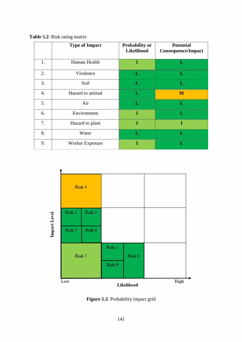
141

Table 5.2: Risk rating matrix

Figure 5.3: Probability impact grid

Type of Impact

Probability or

Likelihood

Potential

Consequence/Impact

1. Human Health I L

2. Virulence L L

3. Soil L L

4. Hazard to animal L M

5. Air L L

6. Environment I L

7. Hazard to plant I I

8. Water L L

9. Worker Exposure I L

142

Table 5.3: Planned response (mitigation)

Risk

Probability Mitigation Plan

Low

The use of proper safety precautions, good laboratory practices, and proper

protective clothing and eyewear in industrial settings can influence impact

on workers.

Risk reduction measures are unlikely to be cost-effective.

Medium

Avoid high level of inhalation exposure due to point source releases.

Risk reduction measures will be roughly cost-neutral.

5.6 Microbial Pesticide Name: Bacillus subtilis strain DSM 3256

Identification and Overview

Bacillus subtilis is a ubiquitous, saprophytic, soil bacterium which is thought to contribute to

nutrient cycling due to its ability to produce a wide variety of enzymes. This latter feature of

the microorganism has been commercially exploited for over a decade and has been used for

industrial production of proteases, amylases, antibiotics, and specialty chemicals. The US

EPA agency (1997) has reviewed the production of enzymes using genetically modified B.

subtilis and found no unreasonable risks to human health or the environment from the use of

this microorganism in fermentation facilities. It is not considered pathogenic and does not

possess traits that cause disease.

Historically, B. subtilis was a term given to all aerobic endospore-forming bacilli. Later, B.

subtilis and two closely related species, B. licheniformis, and B. pumilus, were grouped

taxonomically into what was known as the subtilis-group. However, recently methods have

been developed that allow B. subtilis to be distinguished from these other species. B. subtilis

is not a frank human pathogen, but has on several occasions been isolated from human

infections.

Infections attributed to B. subtilis include bacteraemia, endocarditis, pneumonia, and

septicaemia. However, these infections were found in patients in compromised immune

states. There must be immunosuppression of the host followed by inoculation in high

143

numbers before infection with B. subtilis can occur. There also have been several reported

cases of food poisoning attributed to large numbers of B. subtilis contaminated food. B.

subtilis does not produce significant quantities of extracellular enzymes or other factors that

would predispose it to cause infection. Unlike several other species in the genus, B. subtilis is

not consider toxigenic. B. subtilis does produce the extracellular enzyme subtilisin that has

been reported to cause allergic or hypersensitivity reactions in individuals repeatedly exposed

to it (Edberg, 1991).

Human Health Risk Assessment

B. subtilis is considered a Class 1 containment agent under the National Institute of Health

(NIH) guidelines for research involving recombinant DNA molecules (USHHS, 1986). This

microorganism also falls under the Class 1 containment under the European Federation of

Biotechnology guidelines (Frommer et al., 1989)

In an industrial setting with the use of proper safety precautions, good laboratory practices,

and proper protective clothing and eyewear, the potential for infection of workers should be

quite low, as further explained in Table 5.4. The only human health concern for workers in

the fermentation facility is the potential for allergic reactions with chronic exposure to

subtilisin. Overall, B. subtilis has a low degree of virulence (Edberg, 1991; Ihde &

Armstrong, 1973). Although the possibility of human infection is not non-existent, it is low in

the industrial setting where exposure to the bacterium is expected to be low, and where

highly immunocompromised individuals would not be present.

Ecological Risk Assessment

Likewise, the ecological hazards associated with the use of B. subtilis are low. There are

several reports in the literature on the association of B. subtilis with abortions in livestock

(Fossum, Herikstad, Binde, & Pettersen, 1985). However, these few reports indicate that this

association must be fairly rare, and typically, the animals were immunocompromised. In

addition, B. subtilis has not been shown to be a causal agent and is not considered an animal

pathogen (Logan, 1988). Likewise, B. subtilis is not considered a plant pathogen. Although it

produces enzymes such as polygalacturonase and cellulase that are sometimes associated

with the ability to produce soft rot in plant tissue, there are many organisms that are capable

of producing a soft rot when injected beneath the outer protective epidermal layers. The use

of B. subtilis in an industrial setting should not pose an unreasonable risk to human health or

144

the environment as rated in Table 5.5. First, human health and environmental hazards of B.

subtilis are low. Second, the number of microorganisms released from the fermentation

facility is low. In addition, B. subtilis is ubiquitous in the environment, and the releases

expected from the fermentation facilities will not significantly increase populations of this

bacterium in the environment.

Specific data which indicate the survivability of B. subtilis in the atmosphere after release are

currently unavailable. Air releases from fermentor off-gas could potentially result in non-

occupational inhalation exposures due to point source releases. The natural habitat for B.

subtilis is the soil. Therefore, long-term survival in soil may be expected to occur.

In conclusion, the use of B. subtilis in fermentation facilities to produce BS-1 biosurfactants

or specialty chemicals has a low risk. Although not completely innocuous, the industrial use

of B. subtilis presents low risk of adverse effects to human health or the environment. This is

represented in the risk matrix of Figure 5.4 with a response plan in Table 5.6.

145



Insignificant


failures.

Occurrence is thought most unlikely and does not produce toxins.

No comparable occurrence is known.

Low

Infection could occur in immunosuppressed individual or following exposure

to the bacterium. It has a low degree of virulence.

Environmental hazard occurrence is unlikely as the number of

microorganisms released from fermentation facility is low.

Concerns for workers in the fermentation facility is the potential for allergic

reactions or hypersensitivity with high level of exposure is low.

Comparable reports of food poisoning attributed to large number of B.

subtilis contaminated food..

Medium

Could result from predisposing factors in immunosuppression of the affected

animals.

Could be expected to occur in animals already in an immunocompromised


Comparable reports in association with abortion in livestock are fairly rare.


146



Type of Impact

Probability or

Likelihood

Potential

Consequence/Impact

1. Human Health L L

2. Virulence L I

3. Soil L I

4. Hazard to animal L M

5. Water L L

6. Environment I L

7. Hazard to plant L I

8. Food poison L M

9. Worker Exposure L L

147


Risk


Low

The use of proper safety precautions, good laboratory practices, and proper

protective clothing and eyewear in industrial settings can influence impact

on workers.


Medium

Avoid high level of inhalation exposure due to point source releases.

Risk reduction measures will be roughly cost-neutral.

5.7 Microbial Pesticide Name: Paenibacillus polymxya strain DSM 3256

P. polymyxa is a facultatively anaerobic bacterium that is present in many environments and

it’s not known as an animal, plant or human pathogen. P. polymyxa strain DSM 740 share

characteristics with other P. polymyxa strains that occur in the environment. This assessment

will consider the environmental and human health effects associated with this product use

and industrial processes subject to (CEPA, 1999), including releases to the environment

through waste streams and incidental human exposure through environmental media.

Biological and ecological properties

P. polymyxa is a spore-forming bacterium (Priest, 2015). As a facultative anaerobe, it can be

active under anaerobic conditions and thrives in semi-anaerobic environments, and has a

broad host range as a plant growth–promoting bacterium. It is present in many environments

occuring naturally in marine sediments (Lal & Tabacchioni, 2009), and has also been isolated

from various soils and from cultivated olive trees in an organic orchard farm (Blibech 2012),

and other plant and crops (Lal & Tabacchioni, 2009; Raza, Yang, & Shen, 2008).

Effects on the environment

In agricultural ecosystems in spite of the well-accepted role of P. polymyxa as a plant

growth–promoting bacterium, a few studies have shown that it can also act as a deleterious

rhizobacterium under certain circumstances which resulted in reduction of plant growth and

stunted root system (Timmusk, 2003; Timmusk & Wagner, 1999). It is also known to cause

148

blight in tomato seedlings (Caruso, Zuck, & Bessette, 1984). A comprehensive scientific

literature search did not reveal any further reports of P. polymyxa or

other Paenibacillus species in association with aquatic plants.

Effects on human health

Thus far, there are only two reports associated with human infection involving P. polymyxa,

one involving self-injection of a polymicrobial product containing P. polymyxa and the other

involving a serious comorbidity (pre-existing health condition or disorder) (Galanos et al.,

2003; Nasu et al., 2003). Taken together with the ubiquity of this organism, the significance

of these two cases appears to be negligible. In the unlikely event of P. polymyxa infection,

there are effective antibiotic treatments available (Galanos et al., 2003). However,

other Paenibacillus species occasionally cause disease in humans or are isolated from clinical

samples (K. K. Kim et al., 2010; Ouyang et al., 2008).

Hazard severity

There is little information in the literature to suggest that P. polymyxa is pathogenic to

aquatic or terrestrial plants, vertebrates or invertebrates, in spite of its widespread distribution

in the environment. No reports of animal or plant diseases are attributed to P.

polymyxa strains DSM 740. As discussed previously, P. polymyxa appears to have a history

of safe use based on the range of products known to be in commerce and on an absence of

reports of adverse effects. A few experimental challenge studies have suggested some

potential for adverse effects in plants when directly inoculated with high concentrations of P.

polymyxa (Timmusk (El-Hadad et al., 2011; Liu, Dai, Wu, Li, & Liu, 2012; Timmusk,

Grantcharova, & Wagner, 2005), Blibech et al. 2012. The environmental and human hazard

severity for P. polymyxa strains is therefore estimated to be low.

Sources of exposure

Based on disposal of produced water into the sea, it could likely introduce the strain into

aquatic and terrestrial ecosystems. The magnitude of plant and animal exposure to P.

polymyxa will depend on their persistence and survival in the environment. P. polymyxa is an

endospore-forming facultative anaerobe, capable of thriving in environments with limited

oxygen availability. This explains its ubiquity in soils and in the rhizosphere of various plants

as well as in deeper sub-surface zones in marine sediments. Although this evidence suggests

that P. polymyxa strains introduced to soil and water will likely decrease to background levels

149

over time. Under sub-optimal conditions the spores of P. polymyxa strains are likely to persist

and could accumulate in the environment (Providenti et al., 2009).

Human exposure is expected primarily through direct contact with consumer products

containing P. polymyxa. Secondary to product application, residual P. polymyxa DSM 740 on

surfaces and in reservoirs such as treated drains could result in dermal exposure, as well as

exposure through inadvertent ingestion where the organism persists on food preparation

surfaces and through inhalation where aerosols are generated.

Indirect exposure to P. polymyxa in the environment subsequent to its use in water and

wastewater treatment or produced water disposal, or disposal of waste from its use in the

production of enzymes is also likely to occur in the vicinity of application or disposal sites. In

the event that the organisms enter municipal drinking water treatment systems through

release from potential uses, the water treatment process, which includes coagulation,

flocculation, ozonation, filtration and chlorination, is expected to effectively eliminate these

micro-organisms from drinking water.

Risk Characterization

In this assessment, risk is characterized according to a model embedded in section 64 of

CEPA 1999, that a hazard and exposure to that hazard are both required for there to be a risk.

The risk assessment conclusion is based on the hazard, and on what is known about exposure

from current uses. Hazard has been estimated for P. polymyxa DSM 740 to be low for the

environment and low for human health. Exposures to P. polymyxa DSM 740 from its

deliberate use in industrial processes or consumer or commercial products is not currently

expected (low exposure), so the risk associated with current uses is estimated to be low for

both the environment and human health. The determination of risk from current uses is

followed by consideration of the estimated hazard in relation to foreseeable future exposures.

P. polymyxa DSM 740 have useful properties that make them of interest for use in additional

industrial processes or consumer or commercial products. In the event that potential

consumer, commercial or industrial uses of P. polymyxa is realized, the level of

environmental and human exposure to this strain could increase. Nevertheless, the risk from

foreseeable potential uses of P. polymyxa remains low, given that there is no evidence of

effects on human health or adverse ecological effects at the population level for

150

environmental species, despite widespread distribution of P. polymyxa in the environment

and the history of industrial, environmental and commercial uses of strains DSM 740.

The release of these strains into the environment is not expected to adversely affect

ecosystems. Therefore, in conclusion, based on the information presented in this assessment,

P. polymyxa strains DSM 740 is not entering the environment in a quantity or concentration

or under conditions that:

have or may have an immediate or long-term harmful effect on the environment or its

biological diversity;

constitute or may constitute a danger to the environment on which life depends; or

constitute or may constitute a danger to human life or health.

Therefore, it is concluded that this substance does not meet the criteria as set out in section 64

of CEPA 1999, and therefore, the use of BS-3 biosurfactant in Chapter-4 did not result in any

human risk.

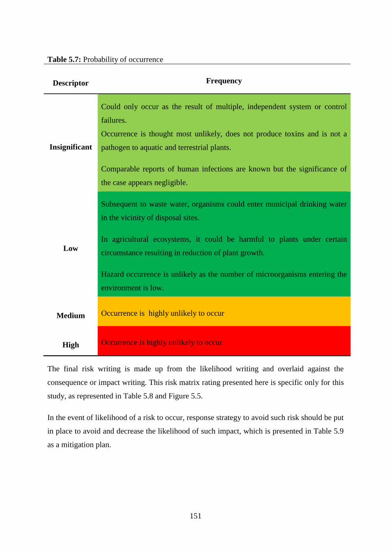
151



Insignificant


failures.

Occurrence is thought most unlikely, does not produce toxins and is not a

pathogen to aquatic and terrestrial plants.

Comparable reports of human infections are known but the significance of

the case appears negligible.

Low

Subsequent to waste water, organisms could enter municipal drinking water

in the vicinity of disposal sites.

In agricultural ecosystems, it could be harmful to plants under certain

circumstance resulting in reduction of plant growth.

Hazard occurrence is unlikely as the number of microorganisms entering the

environment is low.

Medium Occurrence is highly unlikely to occur


The final risk writing is made up from the likelihood writing and overlaid against the

consequence or impact writing. This risk matrix rating presented here is specific only for this

study, as represented in Table 5.8 and Figure 5.5.

In the event of likelihood of a risk to occur, response strategy to avoid such risk should be put

in place to avoid and decrease the likelihood of such impact, which is presented in Table 5.9

as a mitigation plan.

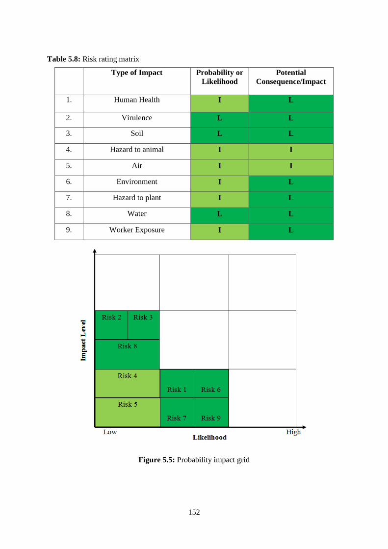
152



Type of Impact

Probability or

Likelihood

Potential

Consequence/Impact

1. Human Health I L

2. Virulence L L

3. Soil L L

4. Hazard to animal I I

5. Air I I

6. Environment I L

7. Hazard to plant I L

8. Water L L

9. Worker Exposure I L

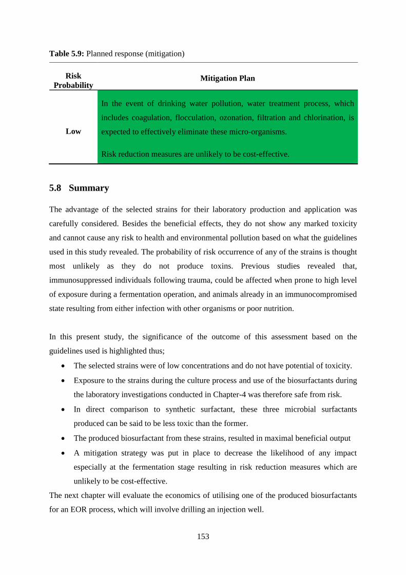
153


Risk


Low

In the event of drinking water pollution, water treatment process, which

includes coagulation, flocculation, ozonation, filtration and chlorination, is

expected to effectively eliminate these micro-organisms.


5.8 Summary

The advantage of the selected strains for their laboratory production and application was

carefully considered. Besides the beneficial effects, they do not show any marked toxicity

and cannot cause any risk to health and environmental pollution based on what the guidelines

used in this study revealed. The probability of risk occurrence of any of the strains is thought

most unlikely as they do not produce toxins. Previous studies revealed that,

immunosuppressed individuals following trauma, could be affected when prone to high level

of exposure during a fermentation operation, and animals already in an immunocompromised


In this present study, the significance of the outcome of this assessment based on the

guidelines used is highlighted thus;

The selected strains were of low concentrations and do not have potential of toxicity.

Exposure to the strains during the culture process and use of the biosurfactants during

the laboratory investigations conducted in Chapter-4 was therefore safe from risk.

In direct comparison to synthetic surfactant, these three microbial surfactants

produced can be said to be less toxic than the former.

The produced biosurfactant from these strains, resulted in maximal beneficial output

A mitigation strategy was put in place to decrease the likelihood of any impact

especially at the fermentation stage resulting in risk reduction measures which are

unlikely to be cost-effective.

The next chapter will evaluate the economics of utilising one of the produced biosurfactants

for an EOR process, which will involve drilling an injection well.

154

Chapter 6

6 Economic Analysis Using BS-2 Biosurfactant to Enhance Residual Oil

in Nembe field, Niger delta.

6.1 Introduction

Economic optimisation is the ultimate goal of any reservoir engineering management, leading

to the main objective of any business project, which is to evaluate the project economic

value, to estimate the return of investment. This is achieved by firstly carrying out a financial

analysis and secondly the economic analysis quantifying all factors to determine whether the

project is profitable or not. In essence, the purpose of any project economics is to determine

the economic value of the project and to support decision-making. Most projects are

prioritised according to investment alternatives whether there is a need to revise, postpone or

even reject the proposal for financial reasons or other intangible considerations.

The majority of oil companies today are focusing on maximizing the recovery factor (RF)

from their oilfields as well as maintaining an economic oil rate. This is because it is

becoming increasingly difficult to discover new oilfields. The average RF from mature

oilfields around the world is somewhere between 20% and 40% (OECD/IEA, 2008; Sandrea

& Sandrea, 2007). This contrasts with a typical RF from gas fields of between 80% and 90%.

At current production rates existing proven oil reserves will last 54 years (Dudley, 2012).

This is probably as good as it has ever been. Improving oil recovery to that typical of gas

fields could more than double the time for which oil is available or alternatively allow for

increased production rates. This would provide more time for an increasingly energy-hungry

world to develop alternative energy sources and technologies (Muggeridge et al., 2014).

The oil market has been at the centre of economic news over much of the past year: what

should we make of the US shale revolution; how will the rebalancing of the Chinese

economy affect demand; and most obviously, what are the implications of the dramatic fall in

oil prices over the past year or so? The implications of these developments are far reaching.

For policymakers, responding to their impact on the prospects for demand and inflation; for

financial markets, involved in the trading and financing of oil flows; and most fundamentally

of all, for businesses and families across the world that rely on oil to fuel their everyday

businesses and lives. As economists, when faced with questions about the oil market and oil

prices, a natural instinct is to revert to the key principles and beliefs that we think underpin

the operation of the oil market (Dale, 2015).

155

Economic evaluation consists of comparing the costs of a project and the effort needed to

finance it, with the value of the expected benefits, which may not be necessarily monetary in

nature, but non-monetary benefits such as social and environmental benefits are also

considered. To make this comparison as many factors as possible are measured in the same

cash units, this evaluation uses the dollar (US$), since most international business in oil and

gas are quoted in dollar.

6.2 Consideration of Economic Parameters and Assumptions

In order to conduct the economic analysis for drilling the injection well, the following

economic parameters and assumptions were considered in this research based on a case

study.

Amount of biosurfactant required for injection is 5,000 gals

Estimated project life is 5 years

Oil price is US$54.89 per barrel flat, Brent Oil (19/04/2017)

Estimated recoverable reserve, 48 million barrels

Uptime 90%, meaning productivity is 0.9 * 365 days

Depreciation follows a straight-line model

A salvage value of zero is assumed

Cooperate taxes rate, 75%

Cost escalation (Inflation rate) 3% every year

Annual production increased by 2.9%

Real discount rate taken to be 10 %

Royalty taken as zero

Capital Expenditure acquired at year 0, while production starts from year 1

Total Capital Cost for Drilling the Injection Well

Although various studies have taken different approaches to calculating the capital cost

associated with drilling and maintaining wells (Godec, 2011), therefore, for the purpose of

targeting enhanced oil recovery in depleted oil reservoirs, this study used the capital cost

estimate based on a case study of Nembe field, within the Niger Delta, Nigeria. Drilling costs

are somewhat dependent upon the type of formations that must be drilled through in order to

reach the target zones; however, that level of detail is not applicable in this study. The

estimated recoverable reserve is 48 million barrels and current production rate is 31,285.62

156

barrels per day. Although, the well production rate was initially 51,530.68 barrels per day

before depleting to its current rate, hence the need for enhanced recovery. The breakdown of

drilling the injection well or capital expenditure (CAPEX) is shown in Table 6.1.

Table 6.1: Typical cost estimate for drilling an injection well

Unit Total Cost

(%)

Cost $

(Millions of Dollar)

Biosurfactant Production 10 4.52

Pump 10.4 4.17

Surface Equipment 44.5 20.17

Plugging Costs 0.6 0.27

Drilling/Pipping 13.4 6.07

Biosurfactant Storage Plant 6.7 3.04

Power Plant 8.2 3.72

Miscellaneous 6.2 2.81

Total Cost 100.0 45.32

Estimation of operating expenditure (OPEX)

As it is imperative to incur a daily operating expenditure of running the injection well, the

significance of OPEX has no future benefits, and thus needs to be managed not to consume

the profits made. The use of inexpensive and waste substrate for the formulation of

fermentation media, which lower the initial raw material costs involved in the process of

biosurfactant production, needs to be harnessed. A series of financial assumptions was

incorporated that affected the price estimates. The OPEX for this recovery process are

divided into two separate costs. Firstly, the cost of raw materials (feed costs) and secondly,

non-feed costs.

6.2.2.1 Preparation of Biosurfactant

The production of biosurfactant requires the formation media for bacterial cultures and the

broth nutrient agar for growing the bacterial. The main raw materials used for this process are

substrates, microorganism, Luria Broth (LB) and Minimal Salt Medium (MSM). However,

there is difficulty in estimating the individual cost of these raw materials, since the LB and

MSM contain several chemical compounds in g/L. Therefore, a lump estimate of 9.5% of the

157

total capital cost of drilling the injection well was taken as the cost of the raw materials.

When we consider the cost of $45.32 million US dollars in drilling the injection well, the

feed cost is then estimated to be $4,305,400 per year.

The non-feed cost includes expenses like maintenance, wages, utilities and miscellaneous

costs. In the absence of itemized costs, the non-feed cost was taken to be 4.05% of the capital

expenditure and it is estimated to be $1,835,460 per year.

Hence the total operating cost for the entire injection process to enhance oil recovery is the

addition of both the feed (raw materials) and non-feed costs as shown in Table 6.2.

Table 6.2: Annual operating costs

Items Total annual Cost

($)

Raw-material 4,305,400

Non-feed cost 1,835,460

Total 6,140,806

Revenue generated from the sales of Oil produced

Cash inflows are generated by the production of oil. The well of interest has the current

capacity of producing 31,285.62 barrels per day. The well was injected with BS-2 supernatant

biosurfactant and shut-in for a two-month period before commencing production again,

(Kuznet︠so︡v, 1963). The choice of the biosurfactant for this analysis, is due to the results

obtained in Chapter-4 for BS-2 supernatant biosurfactant, which gave the best outcome in all

experimental phase. The essence of closing the well for the time period, was to allow for

adequate reaction between the biosurfactant and oil in the pore spaces, of the formation to

take place, to enable an added recovery. With the current oil price and the additional product

yield, the annual sale of the oil produced is estimated as shown in Table 6.3.

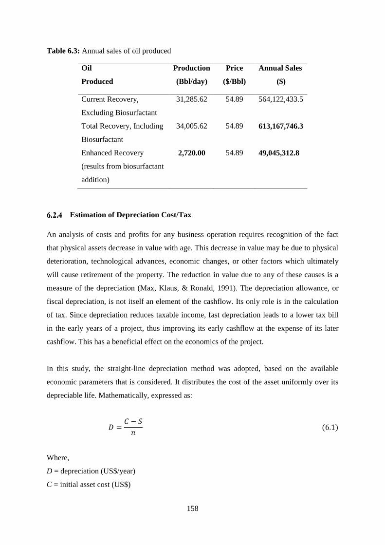
158

Table 6.3: Annual sales of oil produced

Oil

Produced

Production

(Bbl/day)

Price

($/Bbl)

Annual Sales

($)

Current Recovery,

Excluding Biosurfactant

31,285.62 54.89 564,122,433.5

Total Recovery, Including

Biosurfactant

34,005.62 54.89 613,167,746.3

Enhanced Recovery

(results from biosurfactant

addition)

2,720.00 54.89 49,045,312.8

Estimation of Depreciation Cost/Tax

An analysis of costs and profits for any business operation requires recognition of the fact

that physical assets decrease in value with age. This decrease in value may be due to physical

deterioration, technological advances, economic changes, or other factors which ultimately

will cause retirement of the property. The reduction in value due to any of these causes is a

measure of the depreciation (Max, Klaus, & Ronald, 1991). The depreciation allowance, or

fiscal depreciation, is not itself an element of the cashflow. Its only role is in the calculation

of tax. Since depreciation reduces taxable income, fast depreciation leads to a lower tax bill

in the early years of a project, thus improving its early cashflow at the expense of its later

cashflow. This has a beneficial effect on the economics of the project.

In this study, the straight-line depreciation method was adopted, based on the available

economic parameters that is considered. It distributes the cost of the asset uniformly over its

depreciable life. Mathematically, expressed as:

𝐷 =𝐶 − 𝑆

𝑛 (6.1)

Where,

D = depreciation (US$/year)

C = initial asset cost (US$)

159

S = expected salvage value at the end of useful life of asset (US$)

n = estimated useful life of asset (year)

At the end of the project some salvage value can be recovered. The salvage value is a net

amount, net of any removal or dismantling costs but may be very difficult to forecast. If the

net salvage value is small, it can be excluded from the cash flow analysis. Salvage value is

usually positive, which means it is a cash inflow. But there can be cases when the

dismantling and removal costs outweigh the returns from the salvaged asset, thereby

rendering the net salvage value negative. The usual practice is to assume zero salvage value

(Perry & Green, 1999). Hence this value assumed in this study.

For the initial capital investment of $45.32 million and estimate plant life of 5 years, the

depreciation cost is estimated as:

𝐷 = 45.32 − 0

5 (6.2)

= $9.064 Million

The effect of tax on capex/opex/production trade-offs can be very significant. It tends to

make capex more difficult to justify, because the tax relief (through the depreciation

allowance) is deferred and loses Present Value by comparison with the immediate relief on

operating expenditure and the immediate tax on revenue.

6.3 Cash Flow Model

A project or business cash flow is an important financial statement because cash is important

to the survival of a business. This statement reveals the movements of cash over a period and

the effect of these movements of cash position with regards to the economic performance of

the project (McLaney & Atrill, 2015).

A company typical flow of funds is illustrated in Figure 6.1. The excess of sales over

operating costs is called gross profit. From this point, depreciation is deducted, leaving the

taxable income. The taxable income is subjected to state, federal and other fiscal taxes. The

profit remaining after taxes, combined with depreciation is termed cash flow of the venture.

This is the amount of money that goes to the account of the company.

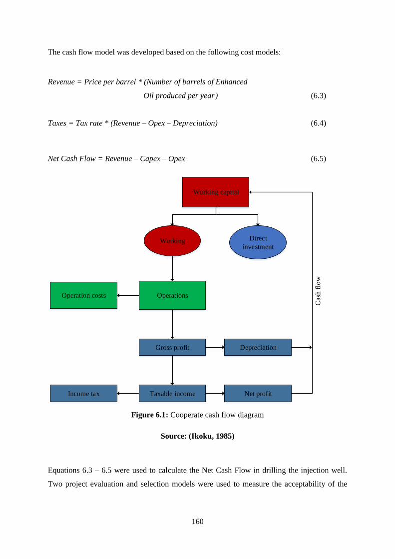
160

The cash flow model was developed based on the following cost models:

Revenue = Price per barrel * (Number of barrels of Enhanced

Oil produced per year ) (6.3)

Taxes = Tax rate * (Revenue – Opex – Depreciation) (6.4)

Net Cash Flow = Revenue – Capex – Opex (6.5)

Working Direct

investment

Working capital

OperationsOperation costs

Gross profit

Taxable income

Depreciation

Net profitIncome tax

Cas

h f

low

Figure 6.1: Cooperate cash flow diagram

Source: (Ikoku, 1985)

Equations 6.3 – 6.5 were used to calculate the Net Cash Flow in drilling the injection well.

Two project evaluation and selection models were used to measure the acceptability of the

161

proposed well in this study. The first was after-tax Net Present Value (NPV) and the later the

Payback period.

6.4 Net Present Value (NPV) Analysis

A project net present value, or alternatively called its present value cash surplus, is the sum

over the years of the project of its discounted cashflow. This represents the value of the

project to the investor. When a project has a positive NPV, it becomes more economically

attractive and the project is likely to be accepted. However, where capital is limited, the

project with the highest NPV is usually accepted. The economic aim in considering

alternatives it to reduce the negative NPV to as low as can be possible.

The net present value realistically predicts the future cash flows against the initial investment.

Mathematically, expressed in Eqn. (6.6). If the project is affected by the impact of

inflation/deflation, then Eqn. (6.6) is modified into Eqn. (6.7) to take care of the impact.

𝑁𝑃𝑉 (𝑝𝑟𝑜𝑗𝑒𝑐𝑡) = 𝐴𝑂 + ∑𝐹𝑡

(1 + 𝑘)𝑡

𝑛

𝑡=1

(6.6)

𝑁𝑃𝑉 (𝑝𝑟𝑜𝑗𝑒𝑐𝑡) = 𝐴𝑂 + ∑𝐹𝑡

(1 + 𝑘 + 𝑝𝑡)𝑡

𝑛

𝑡=1

(6.7)

Where,

Ft = the net cash flow in period t

A0 = initial cash investment (it is negative because it is outflow)

k = the discount rate

pt = predicted rate of inflation/deflation during period t (only if applicable)

t = year of evaluation

n = total number of years of the project life

Investment decisions are based on capital availability; predictions of costs, revenues tax,

inflation, etc.; alternative investments available, attitude to the risks involved. Therefore,

162

appraisal should assess cash flow related to the reject, degree of risk involved and expected

return on investment. Thus, decision-making criteria using NPV are as follows:

where NPV is equal zero or positive, accept the project.

where, NPV is less than zero, reject the project.

In the early life of a project, the net cash is likely to be negative, since the major cash outflow

is the initial investment in the project, A0. The cash flow will be positive if the project is

successful.

6.5 Net Cash Flow of Oil Recovery

Cash flow helps to predict whether the sales or income you forecast will cover the costs of

operation. It also allows you to analyse whether a project will be sufficiently profitable to

justify the effort put into it.

Table 6.4, shows the discounted cash flow generated from drilling the injection well for

enhancing oil recovery using BS-2 supernatant biosurfactant, at 10% discount rate, using

equations 6.3 – 6.7. It can be seen from Table 6.4, that at the end of a five-year period, the

NPV of the project at the discount rate of 10% is $28.340 million, while the cumulative cash

flow was $75.868 million.

163

Table 6.4: Cash flow at 10% discount rate of drilling an injection well

Year

Annual

Revenue

($)

Capex

($)

Opex

($)

Depree

Tax

Net Cash

Flow

(%)

Inflation

Rate

(%)

NPV

($)

Cum. Cash

Flow

($)

0 0 0 0 0 0 0 0 0 0

1 0 45.32 0 0 0 -45.32 0 -41.2 -45.32

2 49.045 45.32 6.14 9.064 22.587 29.382 0.03 23.010 -15.938

3 50.467 45.32 6.14 9.064 22.587 30.804 0.06 19.735 14.866

4 50.496 45.32 6.14 9.064 22.587 30.833 0.09 15.375 45.699

5 50.525 45.32 6.14 9.064 22.587 30.862 0.12 11.419 76.561

Total 200.533

76.561

28.340 75.868

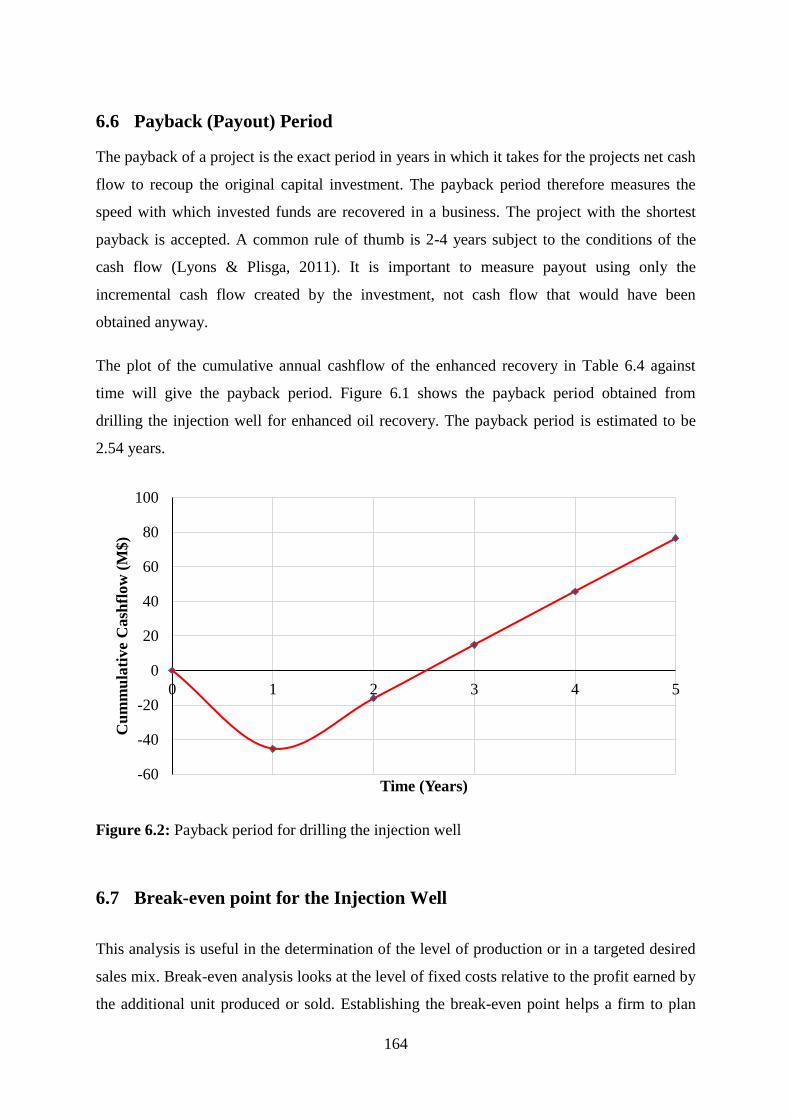
164

6.6 Payback (Payout) Period

The payback of a project is the exact period in years in which it takes for the projects net cash

flow to recoup the original capital investment. The payback period therefore measures the

speed with which invested funds are recovered in a business. The project with the shortest

payback is accepted. A common rule of thumb is 2-4 years subject to the conditions of the

cash flow (Lyons & Plisga, 2011). It is important to measure payout using only the

incremental cash flow created by the investment, not cash flow that would have been

obtained anyway.

The plot of the cumulative annual cashflow of the enhanced recovery in Table 6.4 against

time will give the payback period. Figure 6.1 shows the payback period obtained from

drilling the injection well for enhanced oil recovery. The payback period is estimated to be

2.54 years.

Figure 6.2: Payback period for drilling the injection well

6.7 Break-even point for the Injection Well

This analysis is useful in the determination of the level of production or in a targeted desired

sales mix. Break-even analysis looks at the level of fixed costs relative to the profit earned by

the additional unit produced or sold. Establishing the break-even point helps a firm to plan

-60

-40

-20

0

20

40

60

80

100

0 1 2 3 4 5

Cu

mm

ula

tive

Cash

flow

(M

$)

Time (Years)

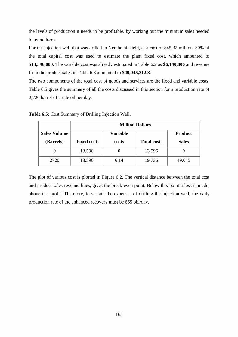
165

the levels of production it needs to be profitable, by working out the minimum sales needed

to avoid loses.

For the injection well that was drilled in Nembe oil field, at a cost of $45.32 million, 30% of

the total capital cost was used to estimate the plant fixed cost, which amounted to

$13,596,000. The variable cost was already estimated in Table 6.2 as $6,140,806 and revenue

from the product sales in Table 6.3 amounted to $49,045,312.8.

The two components of the total cost of goods and services are the fixed and variable costs.

Table 6.5 gives the summary of all the costs discussed in this section for a production rate of

2,720 barrel of crude oil per day.

Table 6.5: Cost Summary of Drilling Injection Well.

Sales Volume

(Barrels)

Million Dollars

Fixed cost

Variable

costs Total costs

Product

Sales

0 13.596 0 13.596 0

2720 13.596 6.14 19.736 49.045

The plot of various cost is plotted in Figure 6.2. The vertical distance between the total cost

and product sales revenue lines, gives the break-even point. Below this point a loss is made,

above it a profit. Therefore, to sustain the expenses of drilling the injection well, the daily

production rate of the enhanced recovery must be 865 bbl/day.

166

Figure 6.3: Break-even graph of enhanced recovery using BS-2 biosurfactant

6.8 Chapter summary

The economic parameters and assumption were established to perform the viability of using

the BS-2 supernatant biosurfactant in an EOR process. All the financial parameters utilised as

a part of this present study, demonstrated that the proposed technique which entails drilling

an injection well for enhancing recovery, is monetarily better and environmentally safe when

used to the oil industry.

A cash flow for the enhanced oil recovered was established, to forecast if the income

generated will cover for the cost of operation. The outcome indicated a payback period of

2.54 years, which may be acceptable for this project.

The cumulative cash flow of US$75,868,000 million dollars was generated by the proposed

injection well. The results also showed that the generated revenue at the end of the estimated

project life, has over 75% influence on the profitability of the project.

The next chapter will give comprehensive conclusion on the findings of this research and

give some future recommendation that could be further studied.

0

10

20

30

40

50

60

0 500 1000 1500 2000 2500 3000

Mil

lio

n D

oll

ars

Sales Volume(Bbls)

Fixed cost Variable cost Total cost Product sales

167

Chapter 7

Conclusions and Future Works

7.1 Conclusions

The experimental methodology utilised in this study gave the main impact and outcome, and

the proposed biosurfactant has been demonstrated to be capable of enhancing residual oil in a

heavy oil reservoir.

A detailed review and discussion of the main mechanisms of MEOR was presented in

Chapter 2, and the significance of wettability in EOR was also discussed. Furthermore,

discussed in Chapter 2 was theoretical background of the pendant drop interfacial tension tool

that was used to quantitatively investigate the effect of the biosurfactants on IFT and contact

angle. Chapter 3 provided a detailed description of the experimental equipment, materials and

procedure used during this experimental work. These procedures followed the conventional

and widely accepted standard protocols outlined in the literature, and at the same time were

modified to achieve the objectives set for this study.

The results of the various concluded experiments were included, interpreted and analysed in

Chapter 4. The effects of the main MEOR mechanisms were also discussed in-line with the

results obtained. Chapter 5, provided a detailed risk assessment of the three strains utilised in

this study in producing the biosurfactants, based on some specific guidelines. The economic

analysis of the proposed injection well was also carried out in Chapter 6, to determine the

profitability of the proposed method.

Based on the findings from this present study, it can be stated that the potential to enhance oil

recovery by these biosurfactants are considerable. All the above work led to the conclusion

that are listed in the different phases below.

Phase – I (Microbial culture)

The selected bacteria strains were successfully extracted from freeze dried conditions,

cultured, inoculated and grown at different temperatures to produce biosurfactants. The

phynotypic characteristic of the bacteria were initially determined, and further sequencing of

the strain using PCR to amplify their DNA, using the forward and reverse primers. The

biosurfactants produced in this present study were named; BS-1, BS-2 and BS-3 respectively.

168

Phase – II (Interfacial tension and contact angle)

The experimental findings of decreasing IFT and contact angle indicated that there was a

considerable reaction between the oil-formation water-biosurfactant interface, which led to

the reduction of intermolecular forces between the oil and formation water at increasing

temperatures.

The produced biosurfactant BS-2 cell-free supernatant gave the best outcome in IFT reduction

and contact angle, against the BS-1 cells with the least performance.

Phase – III (Qualitative wettability tests)

The findings of the qualitative wettability tests revealed that the produced biosurfactants can

decrease the oil wetting of strongly oil-wet Scioto and Bandera Gray sandstones, by changing

the wettability of the surface chemistry of the rock grain to being both water-wet and

intermediate-wet, respectively.

Phase – IV (Core flooding)

The oil recovery increased from 30% to 38% in lesser time from initial water flooding, giving

a recovery factor of 8% after flooding with BS-2 biosurfactant. The increase in oil recovery is

proposed to be due to the biosurfactant changing the wettability of the rock around the

production well.

Chapter 5

Increased environmental awareness has been the main driver for the search for a replacement

to the chemical surfactants. Sucrose, which is a hydrophobic carbon source, was selected as a

suitable carbon nutrient supplement to produce the three biosurfactants. And according to

research findings in the last decade, decomposition property of sucrose makes it eco-friendly

for biosurfactant production.

Chapter 6

The cashflow was discounted at a rate of 10%, which gave a payback period for the proposed

injection well to be 2.54 years. A good knowledge of break-even point for a project can be a

basis for risk assessment. In this analysis, the break-even point has aided to see the volume of

169

daily oil production rates (865 bbl/day), to cover the variable costs and contributing to the

payment of the fixed costs.

7.2 Future Works

The physical characteristics and chemical structure of the biosurfactant produced by

the different strains of Bacillus subtilis BS-1, Bacillus licheniformis BS-2 and

paenibacillus polymyxa BS-3, needed to be determined or identified using mass

spectrometry on each of the samples.

The process for identifying the Critical Micelle Concentration (CMC) is to take

multiple different concentrations of purified surfactant, and measure the surface

tension at each concentration. This process required the use of a DeNouy ring which

was not available and expensive to rent. At the point that the surface tension does not

reduce any lower, this is the point where micelles begin to form and as such is

classified as the CMC using regression analysis. Furthermore, due to the amount of

cell suspension (volume) the equipment requires (reservoir), it would require to make

masses of culture to make enough to create each CMC concentration.

Consideration of the thermal stability and salinity tolerance of the produced

biosurfactants, which also involves the alterations of CMC at different salinities,

temperatures and mineral concentrations of waters. When the CMC increases, the

tolerance is lost at that specific concentration of ion or temperature.

170

References

Abdallah, W., Buckley, J. S., Carnegie, A., Edwards, J., Herold, B., Fordham, E., . . . Signer,

C. (1986). Fundamentals of Wettability. Technology, 38, 1125-1144.

Afrapoli, M. S., Crescente, C., Alipour, S., & Torsaeter, O. (2009). The effect of bacterial

solution on the wettability index and residual oil saturation in sandstone. Journal of

Petroleum Science and Engineering, 69(3-4), 255-260.

doi:10.1016/j.petrol.2009.09.002

AIRMIC, A. (2002). IRM," A Risk Management Standard," The Institute of Risk

Management. Paper presented at the The National Forum for risk Management in the

Public Sector, The Association of Insurance and Risk Managers, London, UK.

Al-Bahry, S., Al-Wahaibi, Y., Elshafie, A., Al-Bemani, A., Joshi, S., Al-Makhmari, H., &

Al-Sulaimani, H. (2013). Biosurfactant production by Bacillus subtilis B20 using date

molasses and its possible application in enhanced oil recovery. International

Biodeterioration & Biodegradation, 81, 141-146.

Al-Hattali, R. (2012). Microbial Biomass for Improving Sweep Efficiency in Fractured

Carbonate Reservoir Using Date Molasses as Renewable Feed Substrate. Paper

presented at the SPE Annual Technical Conference and Exhibition, 8-10 October, San

Antonio, Texas, USA.

Al-Maamari, R. S., & Buckley, J. S. (2003). Asphaltene precipitation and alteration of

wetting: the potential for wettability changes during oil production. SPE Reservoir

Evaluation & Engineering, 6(04), 210-214.

Al-Sulaimani, H., Joshi, S., Al-Wahaibi, Y., Al-Bahry, S., Elshafie, A., & Al-Bemani, A.

(2011). Microbial biotechnology for enhancing oil recovery: current developments

and future prospects. Biotechnol. Bioinf. Bioeng, 1(2), 147-158.

Al-Sulaimani, H. S., Al-Wahaibi, Y. M., Al-Bahry, S., Elshafie, A., Al-Bemani, A. S., Joshi,

S. J., & Zargari, S. (2010). Experimental investigation of biosurfactants produced by

Bacillus species and their potential for MEOR in Omani oil field. Paper presented at

the SPE EOR Conference at Oil & Gas West Asia.

Alvarado, V., & Manrique, E. (2010). Enhanced oil recovery: field planning and

development strategies: Gulf Professional Publishing.

Anderson, W. (1986). Wettability literature survey-Part 1: Rock/oil/brine interactions and the

effects of core handling on wettability. J. Pet. Technol.;(United States), 38(11).

Anderson, W. (1986). Wettability literature survey-part 2: Wettability measurement. Journal

of petroleum technology, 38(11), 1,246-241,262.

Anderson, W. G. (1987a). Wettability literature survey-part 4: Effects of wettability on

capillary pressure. Journal of petroleum technology, 39(10), 1,283-281,300.

Anderson, W. G. (1987b). Wettability literature survey-part 6: the effects of wettability on

waterflooding. Journal of petroleum technology, 39(12), 1,605-601,622.

171

Aronofsky, J. (1952). Mobility ratio-Its influence on flood patterns during water

encroachment. Journal of petroleum technology, 4(01), 15-24.

Ash, C., Priest, F., & Collins, M. (1994). Paenibacillus gen. nov. and Paenibacillus polymyxa

comb. nov. Validation of the publication of new names and new combinations

previously effectively published outside the IJSB, List(51).

Bachmann, R. T., Johnson, A. C., & Edyvean, R. G. (2014). Biotechnology in the petroleum

industry: an overview. International Biodeterioration & Biodegradation, 86, 225-237.

Banat, I., Franzetti, A., Gandolfi, I., Bestetti, G., Martinotti, M., Fracchia, L., . . . Marchant,

R. (2010). Microbial biosurfactants production, applications and future potential.

Applied Microbiology and Biotechnology, 87(2), 427-444. doi:10.1007/s00253-010-

2589-0

Bento, F. M., de Oliveira Camargo, F. A., Okeke, B. C., & Frankenberger, W. T. (2005).

Diversity of biosurfactant producing microorganisms isolated from soils contaminated

with diesel oil. Microbiological research, 160(3), 249-255.

Beveridge, T. J. (2001). Use of the Gram stain in microbiology. Biotechnic & Histochemistry,

76(3), 111-118.

Bond, D. C. (1961). Bacteriological method of oil recovery: Google Patents.

Brown, L. R. (2010). Microbial enhanced oil recovery (MEOR). Curr Opin Microbiol, 13(3),

316-320. doi:http://dx.doi.org/10.1016/j.mib.2010.01.011

Bryant, R. S., & Burchfield, T. E. (1989). Review of Microbial Technology for Improving

Oil Recovery. SPE Reservoir Engineering, 151-154. doi:10.2118/16646-PA

Bryant, R. S., & Douglas, J. (1988). Evaluation of microbial systems in porous media for

EOR. SPE Reservoir Engineering, 3(02), 489-495.

Buckley, J., Liu, Y., & Monsterleet, S. (1998). Mechanisms of wetting alteration by crude

oils. SPE journal, 3(01), 54-61.

Cai, B.-Y., Yang, J.-T., & Guo, T.-M. (1996). Interfacial tension of hydrocarbon+

water/brine systems under high pressure. Journal of chemical & engineering data,

41(3), 493-496.

Campos, J. M., Montenegro Stamford, T. L., Sarubbo, L. A., de Luna, J. M., Rufino, R. D., &

Banat, I. M. (2013). Microbial biosurfactants as additives for food industries.

Biotechnology Progress, 29(5), 1097-1108.

Caruso, F., Zuck, M., & Bessette, A. (1984). Bacterial seedling blight of tomato caused by

Bacillus polymyxa. Plant disease, 68(7), 617-620.

CEPA. (1999). Paenibacillus polymxya https://www.canada.ca/en/environmental-

assessment-agency.html.

Chester, F. D. (1901). A manual of determinative bacteriology: Macmillan Company.

http://dx.doi.org/10.1016/j.mib.2010.01.011

https://www.canada.ca/en/environmental-assessment-agency.html

https://www.canada.ca/en/environmental-assessment-agency.html

172

Dake, L. P. (2001). The practice of reservoir engineering (revised edition) (Vol. 36):

Elsevier.

Dale, S. (2015). New economics of oil.

Davies, J., & Rideal, E. (1963). Interfacial Phenomena, Acad. Press, NY.

Davis, J. B., & Updegraff, D. M. (1954). Microbiology in the petroleum industry.

Bacteriological reviews, 18(4), 215.

De Almeida, D. G., Rita de Cássia, F., Silva, J. M. L., Rufino, R. D., Santos, V. A., Banat, I.

M., & Sarubbo, L. A. (2016). Biosurfactants: Promising Molecules for Petroleum

Biotechnology Advances. Frontiers in Microbiology, 7.

de Guertechin, L. O. (2001). Classification of Surfactants. Handbook of Cosmetic Science

and Technology, Third Edition, 431-450.

de Lima, A. M., & de Souzaa, R. R. (2014). Use of Sugar Cane Vinasse as Substrate for

Biosurfactant Production Using Bacillus subtilis PC. CHEMICAL ENGINEERING,

37.

Desai, J. D., & Banat, I. M. (1997). Microbial production of surfactants and their commercial

potential. Microbiology and Molecular Biology Reviews, 61(1), 47-64.

Deshpande, M., & Daniels, L. (1995). Evaluation of sophorolipid biosurfactant production by

Candida bombicola using animal fat. Bioresource Technology, 54(2), 143-150.

doi:http://dx.doi.org/10.1016/0960-8524(95)00116-6

Dubey, K., & Juwarkar, A. (2004). Determination of genetic basis for biosurfactant

production in distillery and curd whey wastes utilizing Pseudomonas aeruginosa strain

BS2. Indian Journal of Biotechnology, 3(1), 74-81.

Dudley, B. (2012). BP statistical review of world energy. June 2012. London, UK.

Dunlap, C., Schisler, D., Price, N., & Vaughn, S. (2011). Cyclic lipopeptide profile of three

Bacillus subtilis strains; antagonists of Fusarium head blight. The Journal of

Microbiology, 49(4), 603-609. doi:10.1007/s12275-011-1044-y

Dusseault, M. (2001). Comparing Venezuelan and Canadian heavy oil and tar sands. Paper

presented at the Canadian International Petroleum Conference.

Edberg, S. (1991). US EPA human health assessment: Bacillus subtilis. Unpublished, US

Environmental Protection Agency, Washington, DC.

Edwards, U., Rogall, T., Blöcker, H., Emde, M., & Böttger, E. C. (1989). Isolation and direct

complete nucleotide determination of entire genes. Characterization of a gene coding

for 16S ribosomal RNA. Nucleic Acids Research, 17(19), 7843-7853.

El-Hadad, M., Mustafa, M., Selim, S. M., El-Tayeb, T., Mahgoob, A., & Aziz, N. H. A.

(2011). The nematicidal effect of some bacterial biofertilizers on Meloidogyne

incognita in sandy soil. Brazilian Journal of Microbiology, 42(1), 105-113.

http://dx.doi.org/10.1016/0960-8524(95)00116-6

173

El-Sheshtawy, H., Aiad, I., Osman, M., Abo-ELnasr, A., & Kobisy, A. (2015). Production of

biosurfactant from Bacillus licheniformis for microbial enhanced oil recovery and

inhibition the growth of sulfate reducing bacteria. Egyptian Journal of Petroleum,

24(2), 155-162.

Elraies, K. A., & Tan, I. M. (2012). The Application of a New Polymeric Surfactant for

Chemical EOR: INTECH Open Access Publisher.

Fang, X., Wang, Q., Bai, B., Liu, C. X., Tang, Y., Shuler, P. J., & Goddard III, W. A. (2007).

Engineering rhamnolipid biosurfactants as agents for microbial enhanced oil

recovery. Paper presented at the International Symposium on Oilfield Chemistry.

Filho, J. H., Carioca, O. B., Gonzales, R. B., de Lucena, L., & Tavares, C. A. (2012).

Biosurfactants: Production and Utilization in Oil Sludge Cleaning. Paper presented at

the Presented at the SPE EOR Conference at Oil and Gas West Asia held in Muscat,

Oman 16 - 18 April 2012.

Fisher, T. (2016). Phusion DNA Polymerases.

https://www.thermofisher.com/uk/en/home/brands/thermo-scientific/molecular-

biology/thermo-scientific-molecular-biology-products/phusion.html.

Fossum, K., Herikstad, H., Binde, M., & Pettersen, K. (1985). Isolation of Bacillus subtilis in

connection with bovine mastitis. Nordisk veterinaermedicin, 38(4), 233-236.

Friberg, S., & Ahmad, S. (1971). Liquid crystals and the foaming capacity of an amine

dissolved in water and p-xylene. Journal of Colloid and Interface Science, 35(1), 175.

Frommer, W., Ager, B., Archer, L., Brunius, G., Collins, C., Donikian, R., . . . Küenzi, M.

(1989). Safe biotechnology. Applied Microbiology and Biotechnology, 30(6), 541-

552.

Galanos, J., Perera, S., Smith, H., O'Neal, D., Sheorey, H., & Waters, M. J. (2003).

Bacteremia due to three Bacillus species in a case of Munchausen's syndrome.

Journal of Clinical Microbiology, 41(5), 2247-2248.

Godec, M. L. (2011). Global technology roadmap for CCS in industry sectoral assessment

CO2 enhanced oil recovery. Arlington, Virginia.

Griffiths, R. I., Whiteley, A. S., O'Donnell, A. G., & Bailey, M. J. (2000). Rapid method for

coextraction of DNA and RNA from natural environments for analysis of ribosomal

DNA-and rRNA-based microbial community composition. Applied and

environmental microbiology, 66(12), 5488-5491.

Gulick, K. E., & McCain Jr, W. D. (1998). Waterflooding heterogeneous reservoirs: An

overview of industry experiences and practices. Paper presented at the International

Petroleum Conference and Exhibition of Mexico.

Hammershaimb, E., Kuuskraa, V., & Stosur, G. (1983). Recovery efficiency of enhanced oil

recovery methods: a review of significant field tests. Paper presented at the SPE

Annual Technical Conference and Exhibition.

https://www.thermofisher.com/uk/en/home/brands/thermo-scientific/molecular-biology/thermo-scientific-molecular-biology-products/phusion.html

https://www.thermofisher.com/uk/en/home/brands/thermo-scientific/molecular-biology/thermo-scientific-molecular-biology-products/phusion.html

174

Hamouda, A. A., & Karoussi, O. (2008). Effect of temperature, wettability and relative

permeability on oil recovery from oil-wet chalk. Energies, 1(1), 19-34.

Hansen, F. K. (1990). ramé-hart, inc.

Hasiba, H., & Jessen, F. (1968). Film-forming compounds from crude oils, interfacial films

and paraffin deposition. Journal of Canadian Petroleum Technology, 7(01), 1-12.

Hirasaki, G. (1991). Wettability: fundamentals and surface forces. SPE Formation

Evaluation, 6(02), 217-226.

Hsieh, F.-C., Li, M.-C., Lin, T.-C., & Kao, S.-S. (2004). Rapid detection and characterization

of surfactin-producing Bacillus subtilis and closely related species based on PCR.

Current microbiology, 49(3), 186-191.

Ihde, D. C., & Armstrong, D. (1973). Clinical spectrum of infection due to Bacillus species.

The American journal of medicine, 55(6), 839-845.

Ikoku, C. U. (1985). Economic analysis and investment decisions.

Ivanković, T., & Hrenović, J. (2010). Surfactants in the environment. Arhiv za higijenu rada i

toksikologiju, 61(1), 95-109.

Jeong, H., Park, S.-Y., Chung, W.-H., Kim, S. H., Kim, N., Park, S.-H., & Kim, J. F. (2011).

Draft genome sequence of the Paenibacillus polymyxa type strain (ATCC 842T), a

plant growth-promoting bacterium. Journal of Bacteriology, 193(18), 5026-5027.

Johnson, A. (1979). Microbial oil release technique for enhanced oil recovery. Paper

presented at the Proceedings of the Conference on Microbiological Processes Useful

in Enhanced Oil Recovery.

Johnson, S., Salehi, M., Eisert, K., & Fox, S. (2009). Using Biosurfactants Produced from

Agriculture Process Waste Streams to Improve Oil Recovery in Fractured Carbonate

Reservoirs. Retrieved from http://www.osti.gov/scitech//servlets/purl/945026/

Joshi, S., Bharucha, C., Jha, S., Yadav, S., Nerurkar, A., & Desai, A. J. (2008). Biosurfactant

production using molasses and whey under thermophilic conditions. Bioresource

Technology, 99(1), 195-199.

Karimi, M., Mahmoodi, M., Niazi, A., Al-Wahaibi, Y., & Ayatollahi, S. (2012). Investigating

wettability alteration during MEOR process, a micro/macro scale analysis. Colloids

Surf B Biointerfaces, 95, 129-136. doi:10.1016/j.colsurfb.2012.02.035

Kim, H.-S., Jeon, J.-W., Kim, B.-H., Ahn, C.-Y., Oh, H.-M., & Yoon, B.-D. (2006).

Extracellular production of a glycolipid biosurfactant, mannosylerythritol lipid, by

Candida sp. SY16 using fed-batch fermentation. Applied Microbiology and

Biotechnology, 70(4), 391-396. doi:10.1007/s00253-005-0092-9

Kim, K. K., Lee, K. C., Yu, H., Ryoo, S., Park, Y., & Lee, J.-S. (2010). Paenibacillus sputi

sp. nov., isolated from the sputum of a patient with pulmonary disease. International

journal of systematic and evolutionary microbiology, 60(10), 2371-2376.

http://www.osti.gov/scitech/servlets/purl/945026/

175

Kitamoto, D., Ikegami, T., Suzuki, G., Sasaki, A., Takeyama, Y.-i., Idemoto, Y., . . .

Yanagishita, H. (2001). Microbial conversion of n-alkanes into glycolipid

biosurfactants, mannosylerythritol lipids, by Pseudozyma (Candida antarctica).

Biotechnology Letters, 23(20), 1709-1714. doi:10.1023/A:1012464717259

Kowalewski, E., Rueslåtten, I., Steen, K. H., Bødtker, G., & Torsæter, O. (2006). Microbial

improved oil recovery—bacterial induced wettability and interfacial tension effects on

oil production. Journal of Petroleum Science and Engineering, 52(1-4), 275-286.

doi:10.1016/j.petrol.2006.03.011

Kuznetsov, S. (1950). Possibilities of production of methane in oil fields of Saratov and

Buguruslan. Mikrobiologiia, 19(3), 193.

Kuznet︠s︡ov, S. I. (1963). Introduction to geological microbiology: McGraw-Hill.

Lal, S., & Tabacchioni, S. (2009). Ecology and biotechnological potential of Paenibacillus

polymyxa: a minireview. Indian Journal of Microbiology, 49(1), 2-10.

Lazar, I., Petrisor, I., & Yen, T. (2007). Microbial enhanced oil recovery (MEOR). Petroleum

Science and Technology, 25(11), 1353-1366.

Lin, S.-Y., Chen, L.-J., Xyu, J.-W., & Wang, W.-J. (1995). An examination on the accuracy

of interfacial tension measurement from pendant drop profiles. Langmuir, 11(10),

4159-4166.

Liu, R., Dai, M., Wu, X., Li, M., & Liu, X. (2012). Suppression of the root-knot nematode

[Meloidogyne incognita (Kofoid & White) Chitwood] on tomato by dual inoculation

with arbuscular mycorrhizal fungi and plant growth-promoting rhizobacteria.

Mycorrhiza, 22(4), 289-296.

Logan, N. (1988). Bacillus species of medical and veterinary importance. Journal of medical

microbiology, 25(3), 157-165.

Louisajb. (2011). Structure of Surfactin. Wikipedia

https://en.wikipedia.org/wiki/File:Surfactin.png.

Lukondeh, T., Ashbolt, N. J., & Rogers, P. L. (2003). Evaluation of Kluyveromyces

marxianus as a source of yeast autolysates. Journal of Industrial Microbial

Biotechnology, 30, 52-56. doi:10.1007/s10295-002-0008-y

Lyons, W. C., & Plisga, G. J. (2011). Standard handbook of petroleum and natural gas

engineering: Gulf Professional Publishing.

Magot, M. (2005). Indigenous microbial communities in oil fields. Petroleum microbiology.

ASM Press, Washington, DC, 21-33.

Mata-Sandoval, J. C., Karns, J., & Torrents, A. (2001). Effect of nutritional and

environmental conditions on the production and composition of rhamnolipids by P.

aeruginosa UG2.pdf. Microbiology Research, 155, 249-256.

Max, S. P., Klaus, D. T., & Ronald, E. W. (1991). Plant design and economics for chemical

engineers. International edition.

https://en.wikipedia.org/wiki/File:Surfactin.png

176

McCaffery, F. G. (1972). Measurement of interfacial tensions and contact angles at high

temperature and pressure. Journal of Canadian Petroleum Technology, 11(03).

McInerney, M. J., Javaheri, M., & Nagle, D. P., Jr. (1990). Properties of the biosurfactant

produced by Bacillus licheniformis strain JF-2. J Ind Microbiol, 5(2-3), 95-101.

McInerney, M. J., Nagle, D. P., & Knapp, R. M. (2005). Microbially enhanced oil recovery:

past, present, and future Petroleum microbiology (pp. 215-238): American Society of

Microbiology.

McLaney, E., & Atrill, P. (2015). Accounting and Finance: An Introduction 8th edition:

Pearson Higher Ed.

McPhee, C., Reed, J., & Zubizarreta, I. (2015). Core analysis : a best practice guide.

Retrieved from

http://search.ebscohost.com/login.aspx?direct=true&scope=site&db=nlebk&db=nlabk

&AN=1107651

Michaels, A., & Hauser, E. (1951). Interfacial Tension at Elevated Pressure and Temperature.

II. Interfacial Properties of Hydrocarbon–Water Systems. The Journal of Physical

Chemistry, 55(3), 408-421.

Miller, R. G., & Sorrell, S. R. (2014). The future of oil supply: The Royal Society.

Möbius, D., Miller, R., & Fainerman, V. B. (2001). Surfactants: chemistry, interfacial

properties, applications (Vol. 13): Elsevier.

Morrow, N. R. (1990). Wettability and its effect on oil recovery. Journal of petroleum

technology, 42(12), 1,476-471,484.

Muggeridge, A., Cockin, A., Webb, K., Frampton, H., Collins, I., Moulds, T., & Salino, P.

(2014). Recovery rates, enhanced oil recovery and technological limits. Phil. Trans.

R. Soc. A, 372(2006), 20120320.

Muthusamy, K., Gopalakrishnan, S., Ravi, T., & Sivachidambaram. (2008). Biosurfactants

Properties commercial production and application.pdf. Current Science, 94(6), 736.

Myers, D. (1999). Surfaces, interfaces, and colloids: Wiley-Vch New York etc.

Nakamura, L., Roberts, M. S., & Cohan, F. M. (1999). Relationship between the Bacillus

subtilis clades associated with strains 168 and W23: a proposal for B. subtilis subsp.

subtilis and B. subtilis subsp. spizizenii. International journal of systematic

bacteriology, 49, 1211-1215.

Nakano, M. M., Corbell, N., Besson, J., & Zuber, P. (1992). Isolation and characterization of

sfp: a gene that functions in the production of the lipopeptide biosurfactant, surfactin,

in Bacillus subtilis. Molecular and General Genetics MGG, 232(2), 313-321.

Nasu, Y., Nosaka, Y., Otsuka, Y., Tsuruga, T., Nakajima, M., Watanabe, Y., & Jin, M.

(2003). A case of Paenibacillus polymyxa bacteremia in a patient with cerebral

infarction. Kansenshogaku zasshi. The Journal of the Japanese Association for

Infectious Diseases, 77(10), 844-848.

http://search.ebscohost.com/login.aspx?direct=true&scope=site&db=nlebk&db=nlabk&AN=1107651

http://search.ebscohost.com/login.aspx?direct=true&scope=site&db=nlebk&db=nlabk&AN=1107651

177

NCBI. (2016). Primer-Blast. National Centre for Biotechnology Information,

https://blast.ncbi.nlm.nih.gov/Blast.cgi(25th May 2016).

Nicholson, W. L., Munakata, N., Horneck, G., Melosh, H. J., & Setlow, P. (2000). Resistance

of Bacillus endospores to extreme terrestrial and extraterrestrial environments.

Microbiology and Molecular Biology Reviews, 64(3), 548-572.

Nitschke, M., & Pastore, G. M. (2006). Production and properties of a surfactant obtained

from Bacillus subtilis grown on cassava wastewater. Bioresource Technology, 97(2),

336-341. doi:http://dx.doi.org/10.1016/j.biortech.2005.02.044

Noah, K., Bruhn, D., & Bala, G. (2005). Surfactin Production from Potato Process Effluent

by Bacillus subtilis in a Chemostat. In B. Davison, B. Evans, M. Finkelstein, & J.

McMillan (Eds.), Twenty-Sixth Symposium on Biotechnology for Fuels and Chemicals

(pp. 465-473): Humana Press.

OECD/IEA. (2008). World Energy Outlook.

Okasha, T. M., & Alshiwaish, A. (2009). Effect of brine salinity on interfacial tension in

Arab-D carbonate reservoir, Saudi Arabia. Paper presented at the SPE Middle East

Oil and Gas Show and Conference.

Olive, D. M., & Bean, P. (1999). Principles and applications of methods for DNA-based

typing of microbial organisms. Journal of Clinical Microbiology, 37(6), 1661-1669.

Omoregie, E., Ufodike, E., & Onwuliri, C. (1997). Effects of water soluble fractions of crude

oil on carbohydrate reserves of Oreochromis niloticus(L.). Journal of Aquatic

Sciences, 12, 1-7.

Ouyang, J., Pei, Z., Lutwick, L., Dalal, S., Yang, L., Cassai, N., . . . Bluth, M. (2008).

Paenibacillus thiaminolyticus: a new cause of human infection, inducing bacteremia

in a patient on hemodialysis. Annals of Clinical & Laboratory Science, 38(4), 393-

400.

Pacwa-Płociniczak, M., Płaza, G. A., Piotrowska-Seget, Z., & Cameotra, S. S. (2011).

Environmental applications of biosurfactants: recent advances. International Journal

of Molecular Sciences, 12(1), 633-654.

Pathak, K. V., Keharia, H., Gupta, K., Thakur, S. S., & Balaram, P. (2012). Lipopeptides

from the banyan endophyte, Bacillus subtilis K1: mass spectrometric characterization

of a library of fengycins. Journal of the American Society for Mass Spectrometry,

23(10), 1716-1728.

Pekin, G., Vardar-Sukan, F., & Kosaric, N. (2005). Production of Sophorolipids from

Candida bombicola ATCC 22214 Using Turkish Corn Oil and Honey. Engineering in

Life Sciences, 5(4), 357-362. doi:10.1002/elsc.200520086

Perez, A. R., Abanes-De Mello, A., & Pogliano, K. (2000). SpoIIB Localizes to Active Sites

of Septal Biogenesis and Spatially Regulates Septal Thinning during Engulfment in

Bacillus subtilis. Journal of Bacteriology, 182(4), 1096-1108.

https://blast.ncbi.nlm.nih.gov/Blast.cgi(25th

http://dx.doi.org/10.1016/j.biortech.2005.02.044

178

Perfumo, A., Rancich, I., & Banat, I. M. (2010). Possibilities and challenges for

biosurfactants use in petroleum industry Biosurfactants (pp. 135-145): Springer.

Perry, R. H., & Green, D. W. (1999). Perry's chemical engineers' handbook: McGraw-Hill

Professional.

Pichtel, J. (2016). Oil and Gas Production Wastewater: Soil Contamination and Pollution

Prevention. Applied and Environmental Soil Science, 2016.

Polson, E. J., Buckman, J. O., Bowen, D. G., Todd, A. C., Gow, M. M., & Cuthbert, S. J.

(2010). An Environmental-Scanning-Electron-Microscope Investigation Into the

Effect of Biofilm on the Wettability of Quartz. 15(01), 223-227. doi:10.2118/114421-

PA

Priest, F. G. (2015). Paenibacillus. Bergey's Manual of Systematics of Archaea and Bacteria.

Providenti, M. A., Begin, M., Hynes, S., Lamarche, C., Chitty, D., Hahn, J., . . . Smith, M. L.

(2009). Identification and application of AFLP-derived genetic markers for

quantitative PCR-based tracking of Bacillus and Paenibacillus spp. released in soil.

Canadian Journal of Microbiology, 55(10), 1166-1175.

Purwasena, I., Sugai, Y., & Sasaki, K. (2014). Estimation of the potential of an anaerobic

thermophilic oil-degrading bacterium as a candidate for MEOR. Journal of Petroleum

Exploration and Production Technology, 4(2), 189-200. doi:10.1007/s13202-013-

0095-5

Radke, C., Kovscek, A., & Wong, H. (1992). A pore-level scenario for the development of

mixed wettability in oil reservoirs. Paper presented at the SPE Annual Technical

Conference and Exhibition.

Rahman, K. S. M., Rahman, T. J., McClean, S., Marchant, R., & Banat, I. M. (2002).

Rhamnolipid Biosurfactant Production by Strains of Pseudomonas aeruginosa Using

Low-Cost Raw Materials. Biotechnology Progress, 18(6), 1277-1281.

doi:10.1021/bp020071x

Rahman, P. K., & Gakpe, E. (2008). Production, characterisation and applications of

biosurfactants-Review. Biotechnology.

Raz, T., & Hillson, D. (2005). A comparative review of risk management standards. Risk

Management, 7(4), 53-66.

Raza, W., Yang, W., & Shen, Q. (2008). Paenibacillus polymyxa: antibiotics, hydrolytic

enzymes and hazard assessment. Journal of Plant Pathology, 419-430.

Rosenberg, E., & Ron, E. (1999). High-and low-molecular-mass microbial surfactants.

Applied Microbiology and Biotechnology, 52(2), 154-162.

Saharan, B., Sahu, R., & Sharma, D. (2012). A Review on Biosurfactants Fermentation

Current Developments and Perspectives.pdf. Genetic Engineering and Biotechnology,

2011, 1-14.

179

Salathiel, R. (1973). Oil recovery by surface film drainage in mixed-wettability rocks.

Journal of petroleum technology, 25(10), 1,216-211,224.

Salehi, M. (2009). Enhancing the Spontaneous Imbibition Process in Naturally Fractured

Reservoirs through Wettability Alteration Using Surfactant: Mechanistic Study and

Feasibility of Using Biosurfactants Produced from Agriculture Waste Streams.pdf.

PhD Dissertation, University of Kansas, 22-100.

Sandrea, I., & Sandrea, R. (2007). Recovery factors leave vast target for EOR technologies.

Oil & gas journal, 105(41), 44-48.

Santos, D. K. F., Rufino, R. D., Luna, J. M., Santos, V. A., & Sarubbo, L. A. (2016).

Biosurfactants: multifunctional biomolecules of the 21st century. International

Journal of Molecular Sciences, 17(3), 401.

Santos, R., Loh, W., Bannwart, A., & Trevisan, O. (2014). An overview of heavy oil

properties and its recovery and transportation methods. Brazilian Journal of Chemical

Engineering, 31(3), 571-590.

Sarafzadeh, P., Niazi, A., Oboodi, V., Ravanbakhsh, M., Hezave, A. Z., Ayatollahi, S. S., &

Raeissi, S. (2014). Investigating the efficiency of MEOR processes using

Enterobacter cloacae and Bacillus stearothermophilus SUCPM# 14 (biosurfactant-

producing strains) in carbonated reservoirs. Journal of Petroleum Science and

Engineering, 113, 46-53.

Sarubbo, L., Marçal, M., Neves, M., Silva, M., Porto, L., & Campos-Takaki, G. (2001).

Bioemulsifier production in batch culture using glucose as carbon source by Candida

lipolytica. Applied Biochemistry and Biotechnology, 95(1), 59-67.

doi:10.1385/ABAB:95:1:59

Sen, R. (2008). Biotechnology in petroleum recovery: the microbial EOR. Progress in

Energy and Combustion Science, 34(6), 714-724.

Shabani Afrapoli, M., Nikooee, E., Alipour, S., & Torsater, O. (2011). Experimental and

Analytical Study of Microscopic Displacement Mechanisms of MIOR in Porous

Media. Paper presented at the SPE AMericas E & P Health, Safety, Security and

Environmental Conference, Houston, Texas, USA.

Shepherd, R., Rockey, J., Sutherland, I. W., & Roller, S. (1995). Novel bioemulsifiers from

microorganisms for use in foods. Journal of Biotechnology, 40(3), 207-217.

Shibulal, B., Al-Bahry, S. N., Al-Wahaibi, Y. M., Elshafie, A. E., Al-Bemani, A. S., & Joshi,

S. J. (2014). Microbial Enhanced Heavy Oil Recovery by the Aid of Inhabitant Spore-

Forming Bacteria: An Insight Review. The Scientific World Journal, 2014.

Silva, R. d. C. F., Almeida, D. G., Rufino, R. D., Luna, J. M., Santos, V. A., & Sarubbo, L.

A. (2014). Applications of biosurfactants in the petroleum industry and the

remediation of oil spills. International Journal of Molecular Sciences, 15(7), 12523-

12542.

180

Solaiman, D. Y., Ashby, R., Nuñez, A., & Foglia, T. (2004). Production of sophorolipids by

Candida bombicola grown on soy molasses as substrate*,**. Biotechnology Letters,

26(15), 1241-1245. doi:10.1023/B:BILE.0000036605.80577.30

Somasundaran, P., & Zhang, L. (2006). Adsorption of surfactants on minerals for wettability

control in improved oil recovery processes. Journal of Petroleum Science and

Engineering, 52(1–4), 198-212. doi:http://dx.doi.org/10.1016/j.petrol.2006.03.022

Springham, D. G. (1984). Microbiological methods for the enhancement of oil recovery.

Biotechnology and genetic engineering reviews, 1(1), 187-222.

Strassner, J. (1968). Effect of pH on interfacial films and stability of crude oil-water

emulsions. Journal of petroleum technology, 20(03), 303-312.

Sun, X., Zhang, Y., Chen, G., & Gai, Z. (2017). Application of Nanoparticles in Enhanced

Oil Recovery: A Critical Review of Recent Progress. Energies, 10(3), 345.

Taylor, S. E. (2001). Surfactants. Fundamentals and Applications in the Petroleum Industry:

Cambridge University Press; ISBN No.: 0 521 64067 9; Edited by L.L. Schramm,

2000, 621 pp. Journal of Petroleum Science and Engineering, 30(3–4), 258-259.

doi:http://dx.doi.org/10.1016/S0920-4105(01)00115-2

Thanomsub, B., Watcharachaipong, T., Chotelersak, K., Arunrattiyakorn, P., Nitoda, T., &

Kanzaki, H. (2004). Monoacylglycerols: glycolipid biosurfactants produced by a

thermotolerant yeast, Candida ishiwadae. Journal of Applied Microbiology, 96(3),

588-592. doi:10.1111/j.1365-2672.2004.02202.x

Timmusk, S. (2003). Mechanism of action of the plant growth promoting bacterium

Paenibacillus polymyxa. Acta Universitatis Upsaliensis.

Timmusk, S., Grantcharova, N., & Wagner, E. G. H. (2005). Paenibacillus polymyxa invades

plant roots and forms biofilms. Applied and environmental microbiology, 71(11),

7292-7300.

Timmusk, S., & Wagner, E. G. H. (1999). The plant-growth-promoting rhizobacterium

Paenibacillus polymyxa induces changes in Arabidopsis thaliana gene expression: a

possible connection between biotic and abiotic stress responses. Molecular Plant-

Microbe Interactions, 12(11), 951-959.

Trummler, K., Effenberger, F., & Syldatk, C. (2003). An integrated microbial/enzymatic

process for production of rhamnolipids and L-(+)-rhamnose from rapeseed oil with

Pseudomonas sp. DSM 2874. European Journal of Lipid Science and Technology,

105(10), 563-571. doi:10.1002/ejlt.200300816

Updegraff, D., & Wren, G. B. (1954). The release of oil from petroleum-bearing materials by

sulfate-reducing bacteria. Applied microbiology, 2(6), 309.

USHHS. (1986). Bacillus subtilis U.S. Department of Health and Human Services, 1986,

https://www.usa.gov/federal-agencies/u-s-department-of-health-and-human-services.

http://dx.doi.org/10.1016/j.petrol.2006.03.022

http://dx.doi.org/10.1016/S0920-4105(01)00115-2

https://www.usa.gov/federal-agencies/u-s-department-of-health-and-human-services

181

Vance-Harrop, M. H., Gusmão, N. B. d., & Campos-Takaki, G. M. d. (2003). New

bioemulsifiers produced by Candida lipolytica using D-glucose and babassu oil as

carbon sources. Brazilian Journal of Microbiology, 34, 120-123.

Vazquez-Duhalt, R., & Quintero-Ramirez, R. (2004). Biotechnological approach for

development of microbial enhanced oil recovery technique. Petroleum Biotechnology:

Developments and Perspectives, 151, 405 -445.

Venhuis, S. H., & Mehrvar, M. (2004). Health effects, environmental impacts, and

photochemical degradation of selected surfactants in water. International Journal of

photoenergy, 6(3), 115-125.

Wang, W., & Gupta, A. (1995). Investigation of the effect of temperature and pressure on

wettability using modified pendant drop method. Paper presented at the SPE Annual

Technical Conference and Exhibition.

Willey, J. (2008). Prescott, Harley, and Klein's Microbiology-7th international ed./Joanne

M. Willey, Linda M. Sherwood, Christopher J. Woolverton: New York [etc.]:

McGraw-Hill Higher Education.

Wills, M. (2000). Ekologicheskaya Vahkta Sakhalina (Sakhalin Environment Watch Ph. D.

Thesis M. Inst. Petroleum.

Wilson, K., & Walker, J. (2010). Principles and techniques of biochemistry and molecular

biology: Cambridge university press.

Woodward, R. P. (2013). Surface tension measurements using the drop shape method. First

Ten Angstroms), http://www. first tenangstroms. com/pdfdocs/STPaper. pdf. Accessed,

28.

Wu, Y., Shuler, P. J., Blanco, M., Tang, Y., & Goddard, W. A. (2006). A study of wetting

behavior and surfactant EOR in carbonates with model compounds. Paper presented

at the SPE/DOE Symposium on Improved Oil Recovery.

Yang, M.-W., Wei, H.-H., & Lin, S.-Y. (2007). A theoretical study on surfactant adsorption

kinetics: Effect of bubble shape on dynamic surface tension. Langmuir, 23(25),

12606-12616.

Yarbrough, H., & Coty, V. (1983). Microbial enhanced oil recovery from the upper

crustaceous nacatoch formation. Paper presented at the Proceedings of the

International Conference on Microbial Enhancement of Oil Recovery.

Ying, G.-G. (2006). Fate, behavior and effects of surfactants and their degradation products

in the environment. Environment international, 32(3), 417-431.

Zinjarde, S. S., & Pant, A. (2002). Emulsifier from a tropical marine yeast Yarrowia

lipolytica NCIM 3589.pdf. Journal of Basic Microbiology, 42, 67-73.

Zobell, C. E. (1946). Bacteriological process for treatment of fluid-bearing earth formations:

Google Patents.

ZoBell, C. E. (1947). Bacterial release of oil, from oil-bearing materials. World oil, 1, 35-41.

http://www/

182

APPENDICES

Appendix A Journal Publications and Conferences


the impact of biosurfactants on residual-oil recovery. 18th International Conference

on Biological Ecosystems and Ecological Networks, Madrid, Spain, 24 - 25 March

2016.


the impact of biosurfactants on residual-oil recovery. International Journal of

Biological, Biomolecular, Agricultural, Food and Biotechnological

Engineering, 10(3), pp.130-133.

3. Ukwungwu, S.V., Abbas, A.J. and Nasr, G.G., Allison, H., Goodman, S., 2017.

Wettability Effects on Bandera Gray Sandstone using Biosurfactants. Journal of

Engineering Technology. Volume 6, Issue 2, July, 2017, PP.605-617.

183

Appendix B 16S ribosomal RNA gene

184

B1: Bacillus subtilis (DSM 3256), complete sequence

185

B2: Bacillus licheniformis (DSM 1913), complete sequence

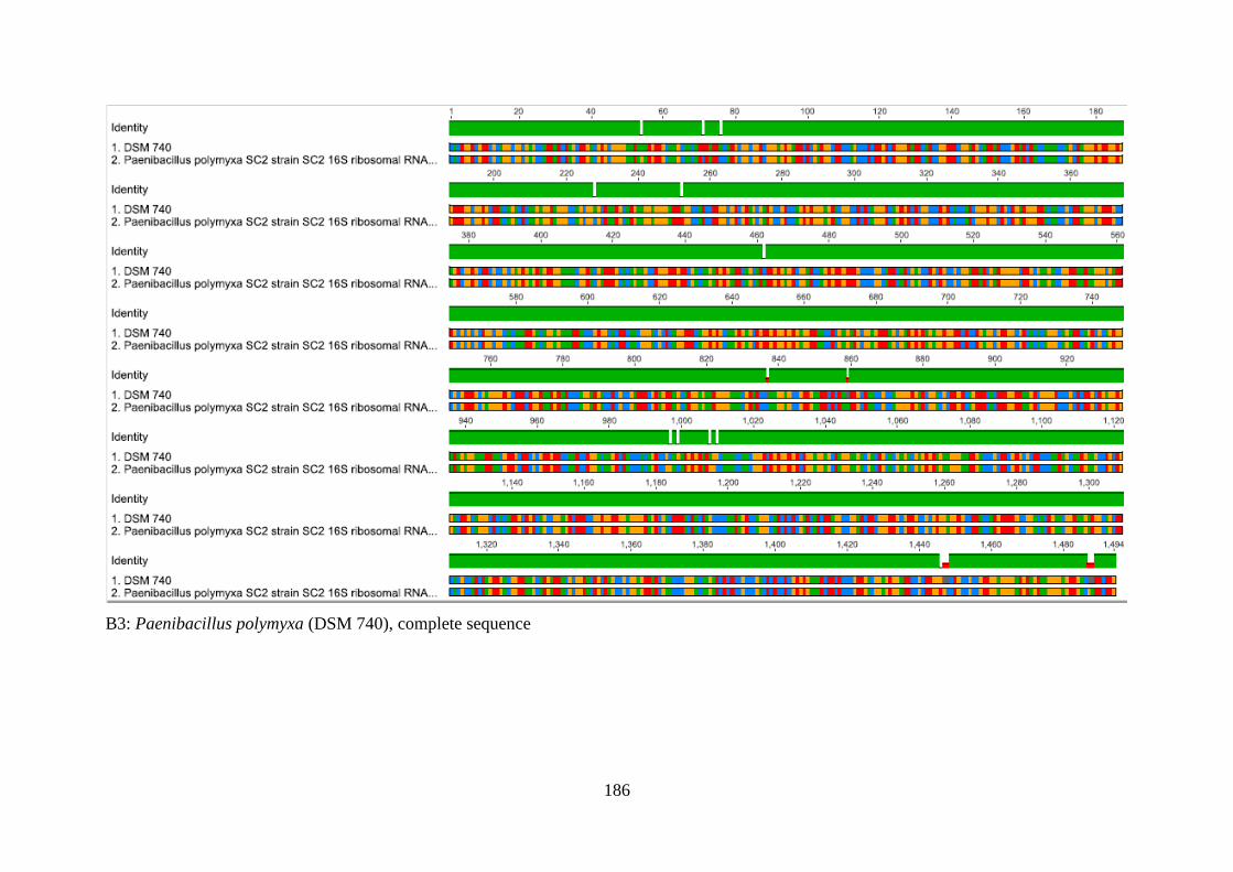
186

B3: Paenibacillus polymyxa (DSM 740), complete sequence

187

Appendix C: The DROPimage program

Using a pendant drop system, it is possible to register the evolution of a drop of oil into

another as a function of time. Images of the drop are taken automatically at a certain

frequency which depends on the time duration of the test. The images are digitized by a

frame grabber resident in the computer and are analysed on line measuring, therefore, the

interfacial tension “on line” during the experiment. The contours of the drops are analysed to

infer interfacial tension from the profile of the drop using different programs. The whole

process of digitization and analysis of the drop lasts less than 40 seconds. It consists of four

steps:

i. capture and digitization of the image of the pendant drop

ii. extraction of the drop contour, determination of the radius of curvature at the apex

necessary for the calculation of interfacial tension

iii. smoothing of the extracted contour of the drop using polynomial regression

iv. shape comparison between the theoretical and experimental drop, inferring the

interfacial tension value.

1. Image display on-screen and real-time

The primary window contains the captured picture. This image is scalable and is utilised to

set the limits and begin position for the edge detection algorithm. The detected edge is also

plotted in this image as a visual sign for the right operation of the edge detection. A real-time

(live) display can be overlaid the primary window, or be shown in a separate window.

After calibrating and setting up the instrument according to the instruction provided, the

micro-syringe assembly is then filled with the test liquid, while the straight needle to the

syringe is attached firmly. The dispensing valve on the micro-syringe is then turned on to

remove air from the needle. The DROPimage Advanced software is then started. The micro-

syringe is adjusted into the fixture so that the tip of the needle is visible in the centre top of

the DROPimage live image as seen as shown below.

188

Visible tip of needle


A new experiment is begun using the experiment Wizard, by clicking on File > New

Experiment Wizard or using the shortcut on the keyboard by hitting Ctrl-T. The dialog box

will appear as shown below.

Setting up a new experiment


The first choice “Surface Tension – Pendant” or third choice “Contact Angle” is selected one

at a time only when the individual experiment is to be conducted. In this case for example we

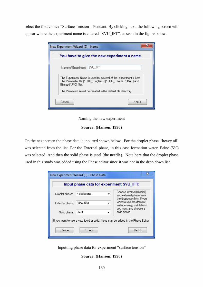
189

select the first choice “Surface Tension – Pendant. By clicking next, the following screen will

appear where the experiment name is entered “SVU_IFT”, as seen in the figure below.

Naming the new experiment


On the next screen the phase data is inputted shown below. For the droplet phase, ‘heavy oil’

was selected from the list. For the External phase, in this case formation water, Brine (5%)

was selected. And then the solid phase is steel (the needle). Note here that the droplet phase

used in this study was added using the Phase editor since it was not in the drop down list.

Inputting phase data for experiment “surface tension”


190

Now the goal of this experiment was to take the average of ten surface tension measurements

over 30 seconds while the drop is at ambient and elevated temperature, humidity and

pressure. After inputting the phase data, on the next screen “10” was entered for the number

of measurements. For the timing, the equidistant option was selected to create a new time file

and the “Time Interval was set to “3” which means that the measurements were taken three

seconds apart, as show below.

Setting data for the experiment’s timing


At this point, on clicking the finish button, the DROPimage will create a Parameter and

Method file for the experiment. And Yes was clicked to run the experiment.

The valve below the cell is then opened to dispense the test liquid in order to produce a

pendant drop (an oil film) as shown below. And as a rule of thumb, you want to use enough

volume to produce a drop that is stable and not so large that it releases itself from the needle,

as can be seen below.

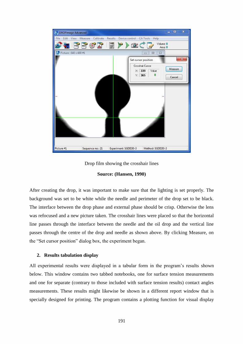
191

Drop film showing the crosshair lines


After creating the drop, it was important to make sure that the lighting is set properly. The

background was set to be white while the needle and perimeter of the drop set to be black.

The interface between the drop phase and external phase should be crisp. Otherwise the lens

was refocused and a new picture taken. The crosshair lines were placed so that the horizontal

line passes through the interface between the needle and the oil drop and the vertical line

passes through the centre of the drop and needle as shown above. By clicking Measure, on

the “Set cursor position” dialog box, the experiment began.

2. Results tabulation display

All experimental results were displayed in a tabular form in the program’s results shown

below. This window contains two tabbed notebooks, one for surface tension measurements

and one for separate (contrary to those included with surface tension results) contact angles

measurements. These results might likewise be shown in a different report window that is

specially designed for printing. The program contains a plotting function for visual display

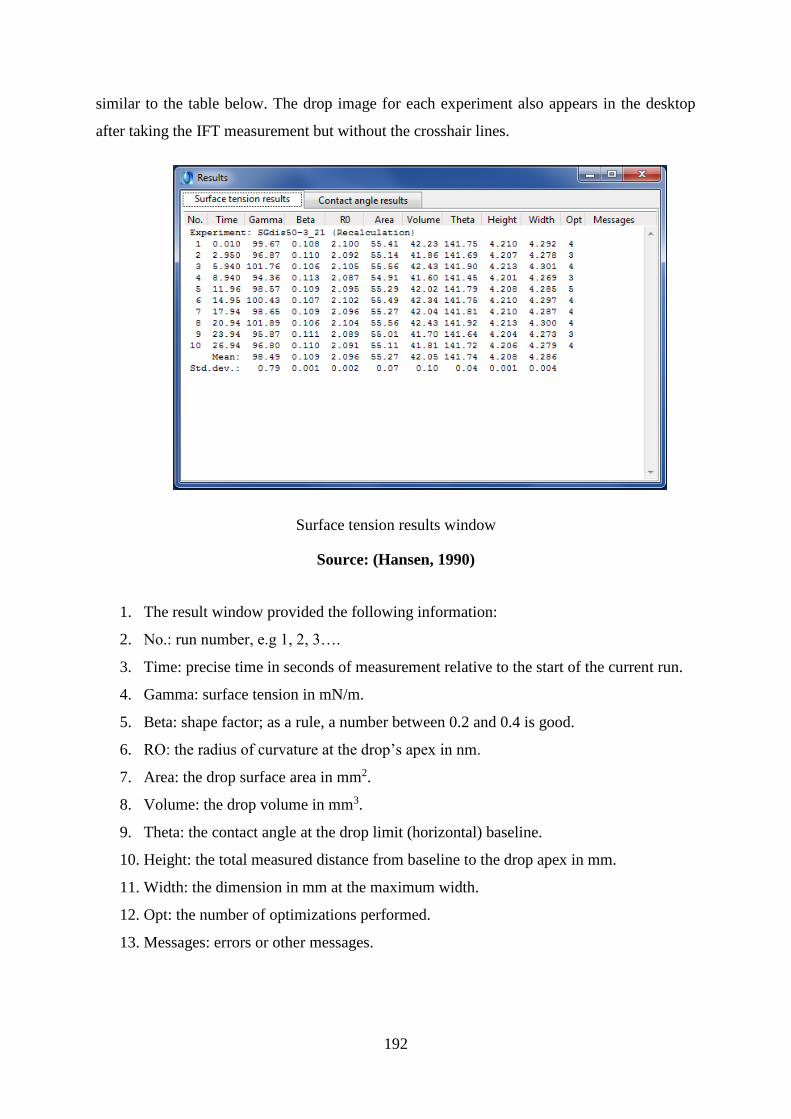
192

similar to the table below. The drop image for each experiment also appears in the desktop

after taking the IFT measurement but without the crosshair lines.

Surface tension results window


1. The result window provided the following information:

2. No.: run number, e.g 1, 2, 3….

3. Time: precise time in seconds of measurement relative to the start of the current run.

4. Gamma: surface tension in mN/m.

5. Beta: shape factor; as a rule, a number between 0.2 and 0.4 is good.

6. RO: the radius of curvature at the drop’s apex in nm.

7. Area: the drop surface area in mm2.

8. Volume: the drop volume in mm3.

9. Theta: the contact angle at the drop limit (horizontal) baseline.

10. Height: the total measured distance from baseline to the drop apex in mm.

11. Width: the dimension in mm at the maximum width.

12. Opt: the number of optimizations performed.

13. Messages: errors or other messages.

193

3. Method Driven Measurement

A method comprises of a collection of parameters that portrays how and when measurements

are made and how results are saved and presented. All measurements of surface tension and

contact angle depend on measurement Methods (aside from single contact angle

measurements). A method’s parameters are saved in a text file. Methods are created and

edited in the Method Editor. All measurement of interfacial tensions must refer to a method,

and quite a lot of measurements can utilise the same method as shown below.

There are basically two sorts of methods, depending on the first field, Data source. In the

event that this is set to Video, data are taken from the edge grabber board for further treatment

as per alternate parameters. On the off chance that Data source is Disk file then this is a

Recalculation method that tells the program to read data from a disk file, which must have

been produced by a method where the data source is Video.

Method editor without the oscillation option.


194

4. Measurement Parameters

Keeping in mind, the end goal is to calculate surface tensions, the program must know the

densities of the two phases (drop and continuous phase), and the image amplification. These

data are saved in a Parameter File seen in the figure below. The parameters are created and

edited in the Parameter Editor. This editor is connected to the Phases data file that contains

the density data of numerous mainstream liquids and gases. This data file is retained in a

different Phase Editor. Notwithstanding the input parameters in the Parameter editor, two

parameters are consequently included from the calibration values. By means of the

measurement parameters, surface tension can be measured by a simple basic methodology

leading to single or multiple readings as indicated by the method in the parameter file.

Parameter editor


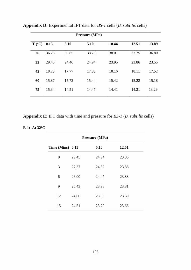
195

Appendix D: Experimental IFT data for BS-1 cells (B. subtilis cells)

Pressure (MPa)

T (oC) 0.15 3.10 5.10 10.44 12.51 13.89

26 36.25 39.85 38.78 38.01 37.75 36.80

32 29.45 24.46 24.94 23.95 23.86 23.55

42 18.23 17.77 17.83 18.16 18.11 17.52

60 15.87 15.72 15.44 15.42 15.22 15.18

75 15.34 14.51 14.47 14.41 14.21 13.29

Appendix E: IFT data with time and pressure for BS-1 (B. subtilis cells)

E-1: At 32oC

Pressure (MPa)

Time (Mins) 0.15 5.10 12.51

0 29.45 24.94 23.86

3 27.37 24.52 23.86

6 26.00 24.47 23.83

9 25.43 23.98 23.81

12 24.66 23.83 23.69

15 24.51 23.70 23.66

196

E-2: At 42oC

Pressure (MPa)

Time (Mins) 0.15 5.10 12.51

0 18.23 17.83 18.11

3 18.08 17.85 18.10

6 17.87 17.86 18.10

9 17.85 17.87 18.11

12 17.81 17.85 18.07

15 17.73 17.86 18.20

E-3: At 75oC

Pressure (MPa)

Time (Mins) 0.15 5.10 12.51

0 15.34 14.47 14.21

3 15.36 14.23 14.01

6 15.14 13.76 13.74

9 14.62 13.56 13.64

12 14.56 13.93 13.64

15 14.50 14.54 13.51

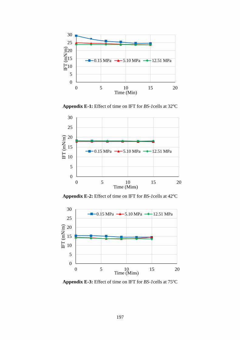
197

Appendix E-1: Effect of time on IFT for BS-1cells at 32oC



0

5

10

15

20

25

30

0 5 10 15 20

IFT

(m

N/m

)

Time (Min)

0.15 MPa 5.10 MPa 12.51 MPa

0

5

10

15

20

25

30

0 5 10 15 20

IFT

(m

N/m

)

Time (Mins)

0.15 MPa 5.10 MPa 12.51 MPa

0

5

10

15

20

25

30

0 5 10 15 20

IFT

(m

N/m

)

Time (Mins)

0.15 MPa 5.10 MPa 12.51 MPa

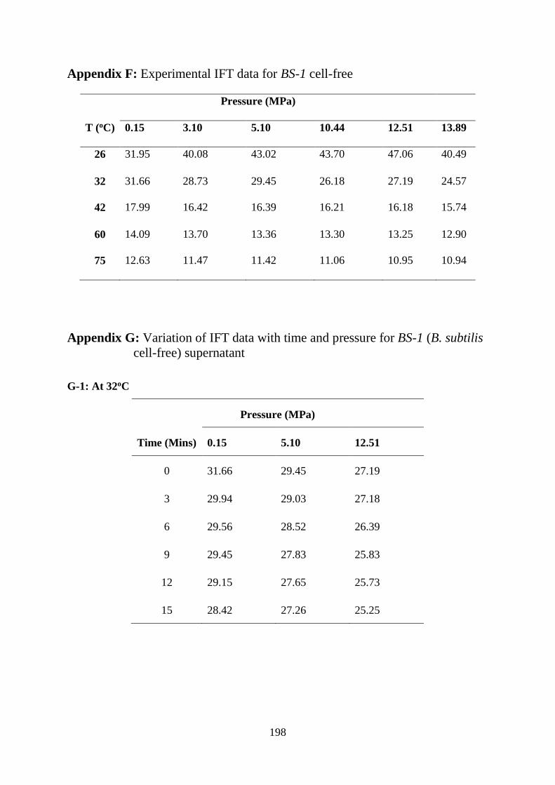
198

Appendix F: Experimental IFT data for BS-1 cell-free

Pressure (MPa)

T (oC) 0.15 3.10 5.10 10.44 12.51 13.89

26 31.95 40.08 43.02 43.70 47.06 40.49

32 31.66 28.73 29.45 26.18 27.19 24.57

42 17.99 16.42 16.39 16.21 16.18 15.74

60 14.09 13.70 13.36 13.30 13.25 12.90

75 12.63 11.47 11.42 11.06 10.95 10.94

Appendix G: Variation of IFT data with time and pressure for BS-1 (B. subtilis

cell-free) supernatant

G-1: At 32oC

Pressure (MPa)

Time (Mins) 0.15 5.10 12.51

0 31.66 29.45 27.19

3 29.94 29.03 27.18

6 29.56 28.52 26.39

9 29.45 27.83 25.83

12 29.15 27.65 25.73

15 28.42 27.26 25.25

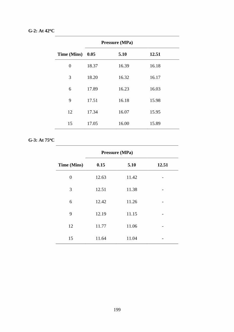
199

G-2: At 42oC

Pressure (MPa)

Time (Mins) 0.05 5.10 12.51

0 18.37 16.39 16.18

3 18.20 16.32 16.17

6 17.89 16.23 16.03

9 17.51 16.18 15.98

12 17.34 16.07 15.95

15 17.05 16.00 15.89

G-3: At 75oC

Pressure (MPa)

Time (Mins) 0.15 5.10 12.51

0 12.63 11.42 -

3 12.51 11.38 -

6 12.42 11.26 -

9 12.19 11.15 -

12 11.77 11.06 -

15 11.64 11.04 -

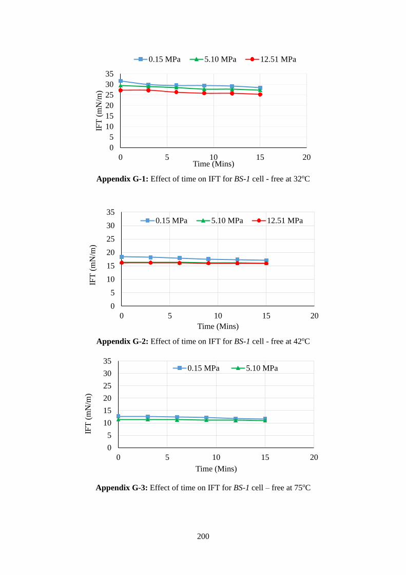
200

Appendix G-1: Effect of time on IFT for BS-1 cell - free at 32oC

Appendix G-2: Effect of time on IFT for BS-1 cell - free at 42oC

Appendix G-3: Effect of time on IFT for BS-1 cell – free at 75oC

0

5

10

15

20

25

30

35

0 5 10 15 20

IFT

(m

N/m

)

Time (Mins)

0.15 MPa 5.10 MPa 12.51 MPa

0

5

10

15

20

25

30

35

0 5 10 15 20

IFT

(m

N/m

)

Time (Mins)

0.15 MPa 5.10 MPa 12.51 MPa

0

5

10

15

20

25

30

35

0 5 10 15 20

IFT

(m

N/m

)

Time (Mins)

0.15 MPa 5.10 MPa

201

Appendix H: IFT with temperature at constant pressure for BS-2 with cells

Appendix I: IFT with time for BS-2 biosurfactant with cells

I-1: At 42oC

Pressure (MPa)

Time (Mins) 0.15 5.10 12.51

0 16.07 14.86 13.97

3 15.26 14.86 13.98

6 15.25 14.8 13.95

9 15.19 14.68 13.9

12 15.18 14.63 13.83

15 15.11 14.55 13.79

Pressure (MPa)

T (oC) 0.15 3.10 5.10 10.44 12.51 13.89

26 23.87 23.12 22.72 22.05 21.89 21.10

32 20.44 20.22 20.11 21.04 20.69 19.49

42 16.07 15.15 14.86 13.98 13.97 13.72

60 13.10 13.18 13.29 13.46 13.39 13.33

75 12.99 12.34 12.12 12.29 11.43 11.37

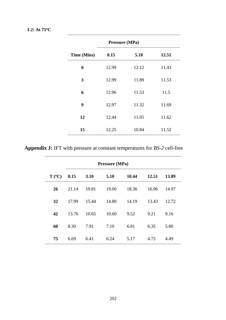
202

I-2: At 75oC

Pressure (MPa)

Time (Mins) 0.15 5.10 12.51

0 12.99 12.12 11.43

3 12.99 11.89 11.53

6 12.96 11.53 11.5

9 12.97 11.32 11.69

12 12.44 11.05 11.62

15 12.25 10.84 11.52

Appendix J: IFT with pressure at constant temperatures for BS-2 cell-free

Pressure (MPa)

T (oC) 0.15 3.10 5.10 10.44 12.51 13.89

26 21.14 19.81 19.06 18.36 16.96 14.97

32 17.99 15.44 14.80 14.19 13.43 12.72

42 13.76 10.65 10.60 9.52 9.21 9.16

60 8.30 7.91 7.10 6.81 6.35 5.80

75 6.69 6.41 6.24 5.17 4.75 4.49

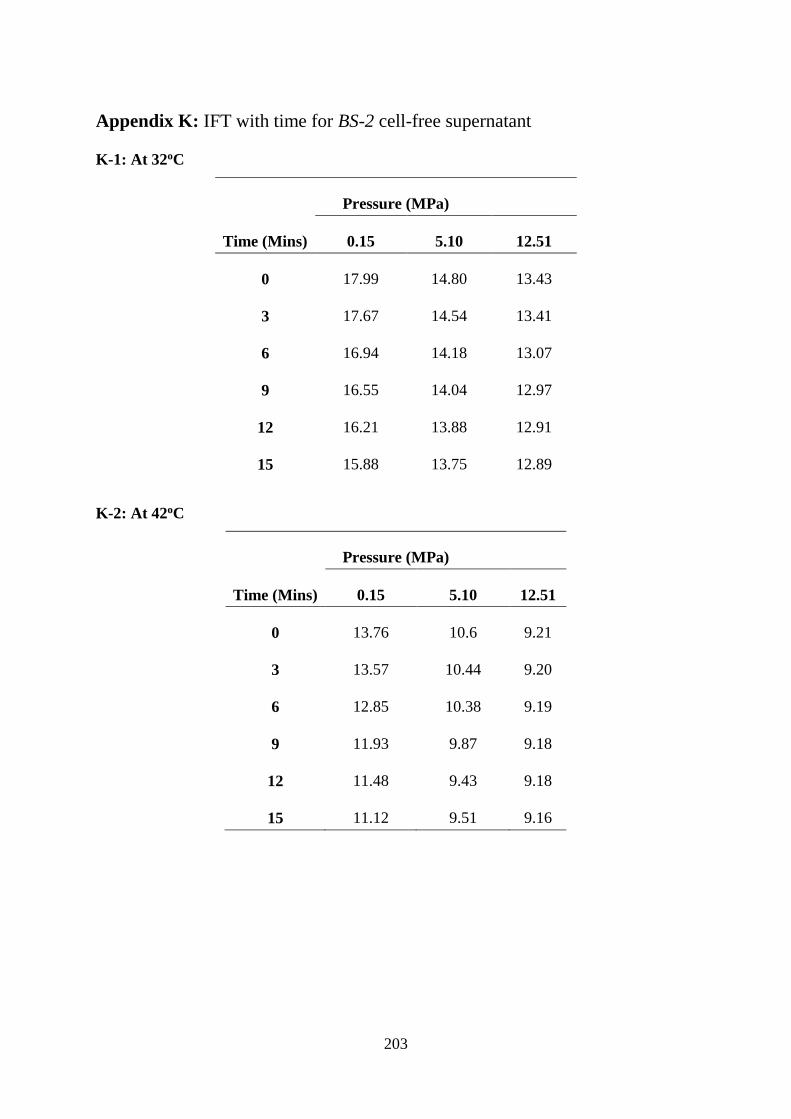
203

Appendix K: IFT with time for BS-2 cell-free supernatant

K-1: At 32oC

Pressure (MPa)

Time (Mins) 0.15 5.10 12.51

0 17.99 14.80 13.43

3 17.67 14.54 13.41

6 16.94 14.18 13.07

9 16.55 14.04 12.97

12 16.21 13.88 12.91

15 15.88 13.75 12.89

K-2: At 42oC

Pressure (MPa)

Time (Mins) 0.15 5.10 12.51

0 13.76 10.6 9.21

3 13.57 10.44 9.20

6 12.85 10.38 9.19

9 11.93 9.87 9.18

12 11.48 9.43 9.18

15 11.12 9.51 9.16

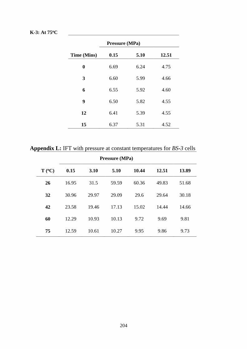
204

K-3: At 75oC

Pressure (MPa)

Time (Mins) 0.15 5.10 12.51

0 6.69 6.24 4.75

3 6.60 5.99 4.66

6 6.55 5.92 4.60

9 6.50 5.82 4.55

12 6.41 5.39 4.55

15 6.37 5.31 4.52

Appendix L: IFT with pressure at constant temperatures for BS-3 cells

Pressure (MPa)

T (oC) 0.15 3.10 5.10 10.44 12.51 13.89

26 16.95 31.5 59.59 60.36 49.83 51.68

32 30.96 29.97 29.09 29.6 29.64 30.18

42 23.58 19.46 17.13 15.02 14.44 14.66

60 12.29 10.93 10.13 9.72 9.69 9.81

75 12.59 10.61 10.27 9.95 9.86 9.73

205

Appendix M: Experimental IFT data for BS-3 cell-free

Pressure (MPa)

T (oC) 0.15 3.10 5.10 10.44 12.51 13.89

26 - - - - - -

32 34.05 22.48 22.32 21.22 19.58 18.75

42 11.42 10.76 10.46 9.75 9.40 8.99

60 8.71 8.70 8.58 8.55 8.38 7.90

75 7.79 7.05 7.37 7.02 6.64 6.62

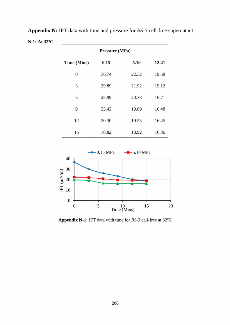
206

Appendix N: IFT data with time and pressure for BS-3 cell-free supernatant

N-1: At 32oC

Pressure (MPa)

Time (Mins) 0.15 5.10 12.41

0 36.74 22.32 19.58

3 29.89 21.92 19.12

6 25.99 20.78 16.71

9 23.42 19.69 16.48

12 20.30 19.55 16.45

15 18.82 18.92 16.36

Appendix N-1: IFT data with time for BS-3 cell-free at 32oC

0

10

20

30

40

0 5 10 15 20

IFT

(m

N/m

)

Time (Mins)

0.15 MPa 5.10 MPa

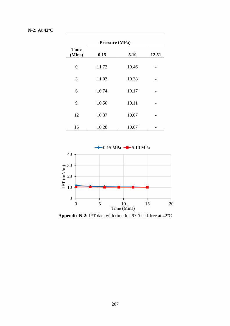
207

N-2: At 42oC

Pressure (MPa)

Time

(Mins) 0.15 5.10 12.51

0 11.72 10.46 -

3 11.03 10.38 -

6 10.74 10.17 -

9 10.50 10.11 -

12 10.37 10.07 -

15 10.28 10.07 -

Appendix N-2: IFT data with time for BS-3 cell-free at 42oC

0

10

20

30

40

0 5 10 15 20

IFT

(m

N/m

)

Time (Mins)

0.15 MPa 5.10 MPa

208

Appendix O: Comparison of IFT with temperature for BS1, BS-2 & BS-3 with

cells

O-1: At 0.15 MPa

Biosurfactant

T (oC) BS-1 BS-2 BS-3

26 36.25 23.87 16.95

32 29.45 20.44 30.96

42 18.23 16.07 23.58

60 15.87 13.10 12.29

75 15.34 12.99 12.59

O-2: At 3.10 MPa

Biosurfactant


26 39.85 23.12 31.50

32 24.46 20.22 29.29

42 17.77 15.15 19.46

60 15.72 13.18 10.93

75 14.51 12.34 10.61

209

O-3: At 5.10 MPa

Biosurfactant

T(oC) BS-1 BS-2 BS-3

26 38.78 22.72 59.69

32 24.94 20.11 29.09

42 17.83 14.86 17.13

60 15.44 13.29 10.13

75 14.47 12.12 10.27

O-4: At 10.44 MPa

Biosurfactant


26 38.01 22.05 60.36

32 23.95 21.04 29.6

42 18.16 13.98 15.02

60 15.42 13.46 9.72

75 14.41 12.29 9.95

210

O-5: At 12.51 MPa

Biosurfactant


26 37.75 21.89 49.83

32 23.86 20.69 29.64

42 18.11 13.97 14.44

60 15.22 13.39 9.69

75 14.21 11.43 9.86

O-6: At 13.89 MPa

Biosurfactant


26 36.8 21.1 51.68

32 23.55 19.49 30.18

42 17.52 13.72 14.66

60 15.18 13.33 9.81

75 13.29 11.37 9.73

211

Appendix P: Comparison of IFT with time for BS-1 & BS-2 biosurfactants with

cells

P-1: At constant temperature 42oC

(a) At constant pressure of 0.15 MPa

(b) At constant pressure of 5.10 MPa

(c) At constant pressure of 12.15 MPa

12

14

16

18

20

0 5 10 15 20

IFT

(m

N/m

)

Time (Mins)

BS 1 BS 2

12

13

14

15

16

17

18

19

20

0 5 10 15 20

IFT

(m

N/m

)

Time (Mins)

BS 1 BS 2

12

13

1415

16

17

18

19

20

0 5 10 15 20

IFT

(m

N/m

)

Time (Mins)

BS 1 BS 2

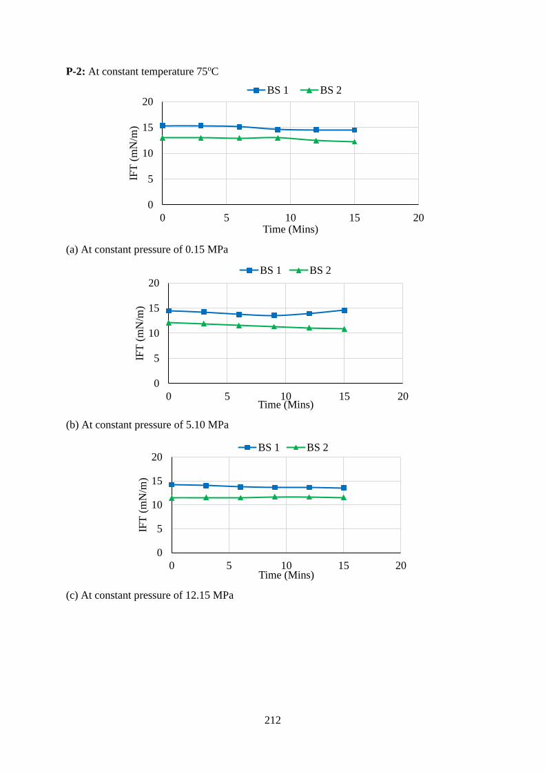
212

P-2: At constant temperature 75oC




0

5

10

15

20

0 5 10 15 20

IFT

(m

N/m

)

Time (Mins)

BS 1 BS 2

0

5

10

15

20

0 5 10 15 20

IFT

(m

N/m

)

Time (Mins)

BS 1 BS 2

0

5

10

15

20

0 5 10 15 20

IFT

(m

N/m

)

Time (Mins)

BS 1 BS 2

213

P-1A: Comparison of IFT with time for cell-free BS-1 & BS-2 biosurfactants at 42oC

At 0.15 MPa

Biosurfactant

Time (Mins) BS-1 BS-2

0 18.23 16.07

3 18.08 15.26

6 17.87 15.25

9 17.85 15.19

12 17.81 15.18

15 17.73 15.11

At 5.10 MPa

Biosurfactant


0 17.83 14.86

3 17.85 14.86

6 17.86 14.80

9 17.87 14.68

12 17.85 14.63

15 17.86 14.55

214

At 12.51 MPa

Biosurfactant


0 18.11 13.97

3 18.10 13.98

6 18.10 13.95

9 18.11 13.90

12 18.07 13.83

15 18.20 13.79

P-2B: Comparison of IFT with time for cell-free BS-1 & BS-2 biosurfactants at 75oC

At 0.15 MPa

Biosurfactant


0 15.34 12.99

3 15.36 12.99

6 15.14 12.96

9 14.62 12.97

12 14.56 12.44

15 14.5 12.25

215

At 5.10 MPa

Biosurfactant


0 14.47 12.12

3 14.23 11.89

6 13.76 11.53

9 13.56 11.32

12 13.93 11.05

15 14.54 10.84

At 12.51 MPa

Biosurfactant


0 14.21 11.43

3 14.01 11.53

6 13.74 11.5

9 13.64 11.69

12 13.64 11.62

15 13.51 11.52

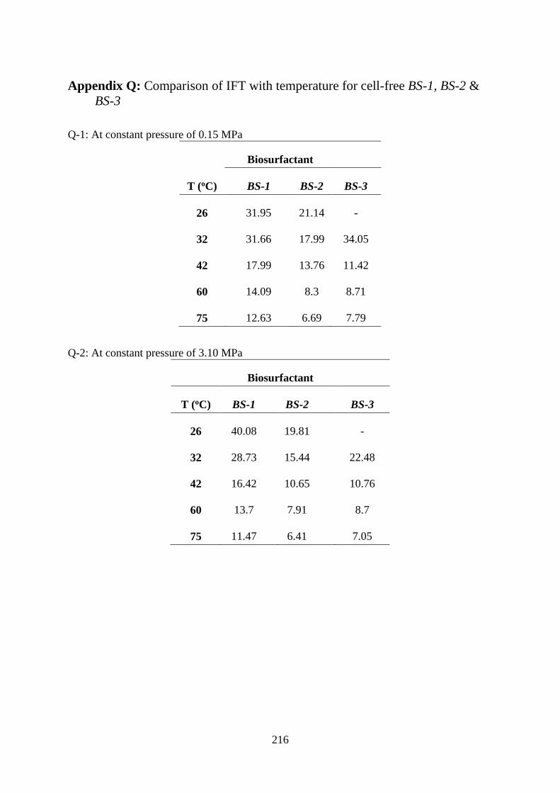
216

Appendix Q: Comparison of IFT with temperature for cell-free BS-1, BS-2 &

BS-3

Q-1: At constant pressure of 0.15 MPa

Biosurfactant


26 31.95 21.14 -

32 31.66 17.99 34.05

42 17.99 13.76 11.42

60 14.09 8.3 8.71

75 12.63 6.69 7.79


Biosurfactant


26 40.08 19.81 -

32 28.73 15.44 22.48

42 16.42 10.65 10.76

60 13.7 7.91 8.7

75 11.47 6.41 7.05

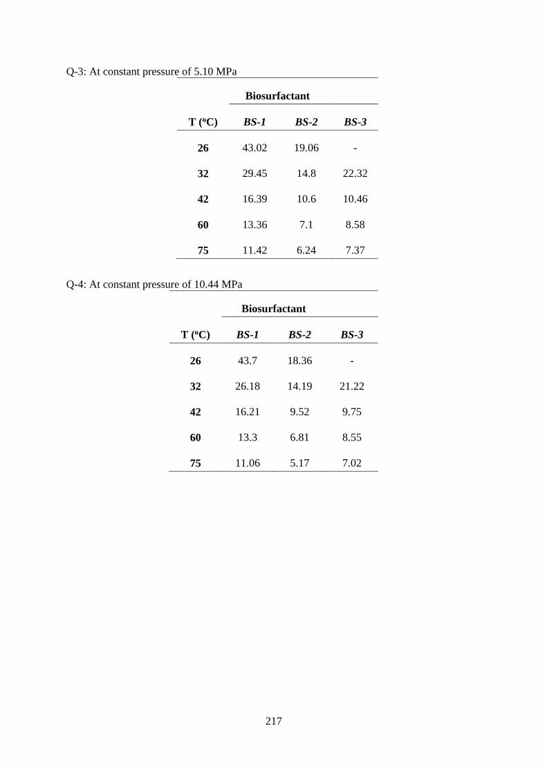
217


Biosurfactant


26 43.02 19.06 -

32 29.45 14.8 22.32

42 16.39 10.6 10.46

60 13.36 7.1 8.58

75 11.42 6.24 7.37


Biosurfactant


26 43.7 18.36 -

32 26.18 14.19 21.22

42 16.21 9.52 9.75

60 13.3 6.81 8.55

75 11.06 5.17 7.02

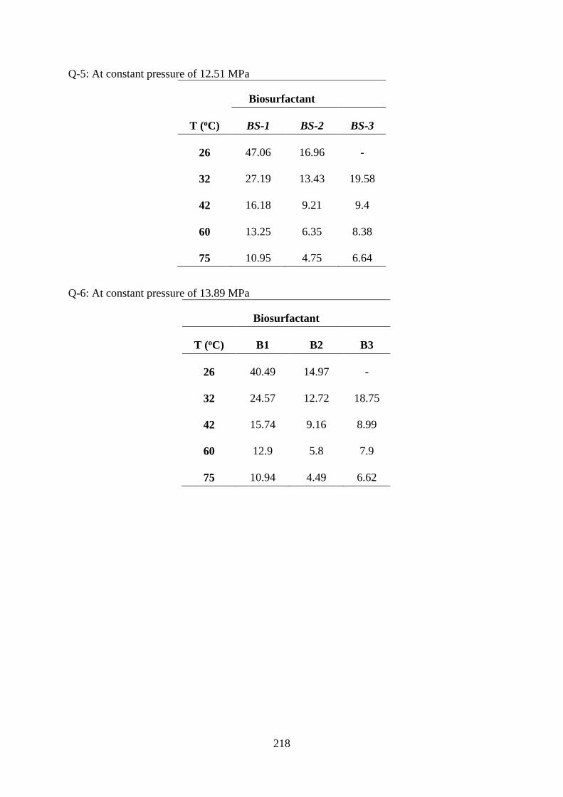
218


Biosurfactant


26 47.06 16.96 -

32 27.19 13.43 19.58

42 16.18 9.21 9.4

60 13.25 6.35 8.38

75 10.95 4.75 6.64


Biosurfactant

T (oC) B1 B2 B3

26 40.49 14.97 -

32 24.57 12.72 18.75

42 15.74 9.16 8.99

60 12.9 5.8 7.9

75 10.94 4.49 6.62

219

Appendix R: Comparison of IFT with time for cell-free biosurfactants

R-1: At temperature of 32oC

At 0.15 MPa

Biosurfactant

Time (Mins) BS-1 BS-2 BS-3

0 31.66 17.99 36.74

3 29.94 17.67 29.89

6 29.56 16.94 25.99

9 29.45 16.55 23.42

12 29.15 16.21 20.3

15 28.42 15.88 18.82


0

10

20

30

40

0 5 10 15 20

IFT

(m

N/m

)

Time (Mins)

BS 1 BS 2 BS 3

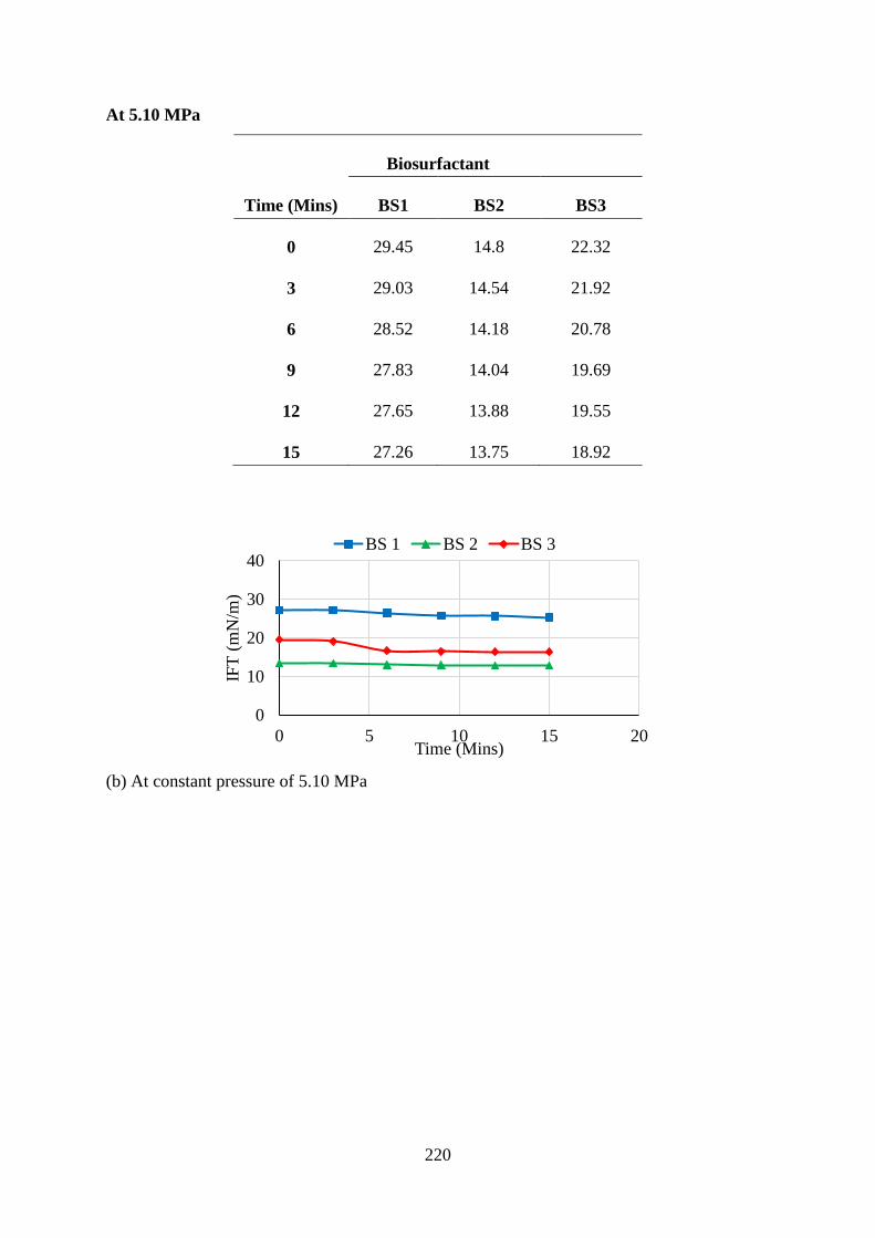
220

At 5.10 MPa

Biosurfactant

Time (Mins) BS1 BS2 BS3

0 29.45 14.8 22.32

3 29.03 14.54 21.92

6 28.52 14.18 20.78

9 27.83 14.04 19.69

12 27.65 13.88 19.55

15 27.26 13.75 18.92


0

10

20

30

40

0 5 10 15 20

IFT

(m

N/m

)

Time (Mins)

BS 1 BS 2 BS 3

221

At 12.15 MPa

Biosurfactant


0 27.19 13.43 19.58

3 27.18 13.41 19.12

6 26.39 13.07 16.71

9 25.83 12.97 16.48

12 25.73 12.91 16.45

15 25.25 12.89 16.36


0

10

20

30

40

0 5 10 15 20

IFT

(m

N/m

)

Time (Mins)

BS 1 BS 2 BS 3

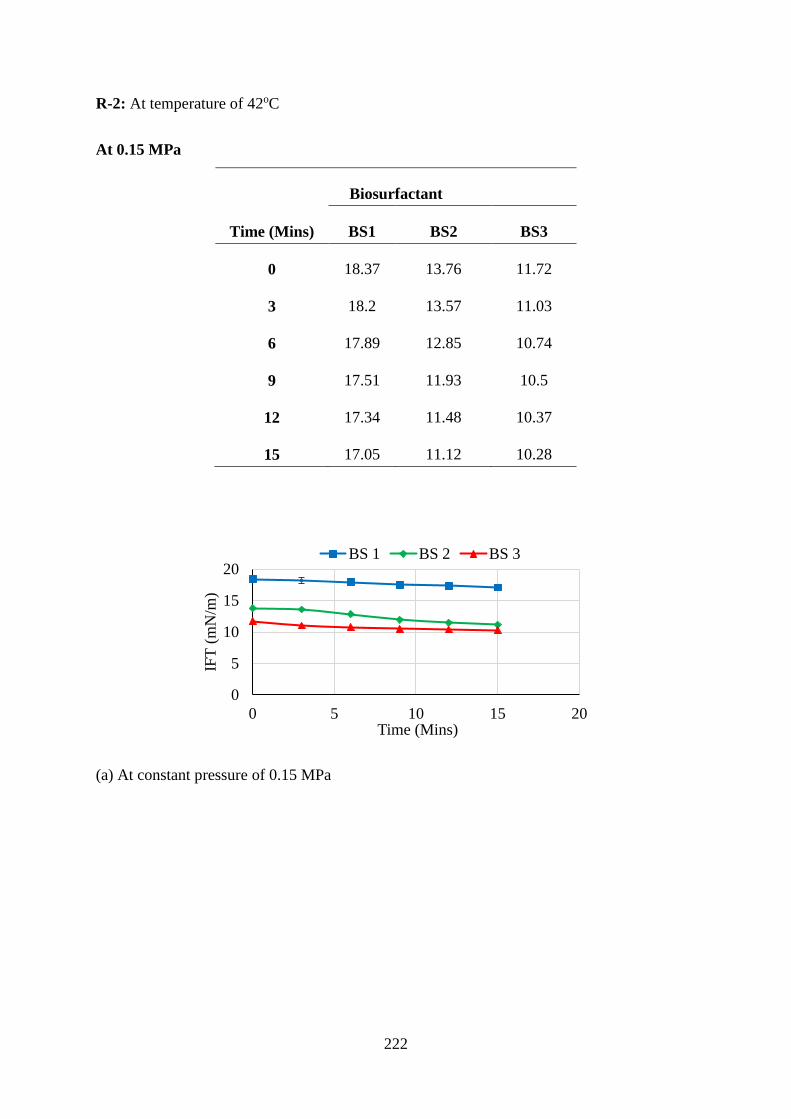
222


At 0.15 MPa

Biosurfactant

Time (Mins) BS1 BS2 BS3

0 18.37 13.76 11.72

3 18.2 13.57 11.03

6 17.89 12.85 10.74

9 17.51 11.93 10.5

12 17.34 11.48 10.37

15 17.05 11.12 10.28


0

5

10

15

20

0 5 10 15 20

IFT

(m

N/m

)

Time (Mins)

BS 1 BS 2 BS 3

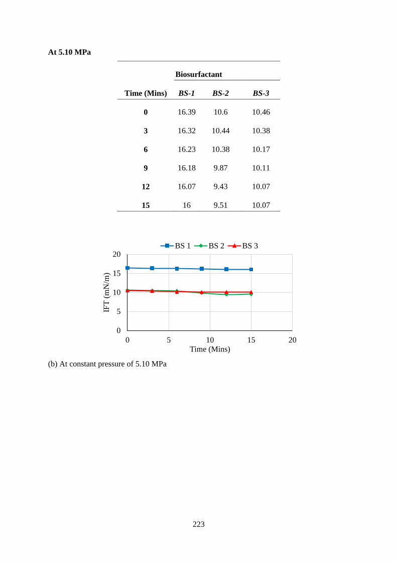
223

At 5.10 MPa

Biosurfactant


0 16.39 10.6 10.46

3 16.32 10.44 10.38

6 16.23 10.38 10.17

9 16.18 9.87 10.11

12 16.07 9.43 10.07

15 16 9.51 10.07


0

5

10

15

20

0 5 10 15 20

IFT

(m

N/m

)

Time (Mins)

BS 1 BS 2 BS 3

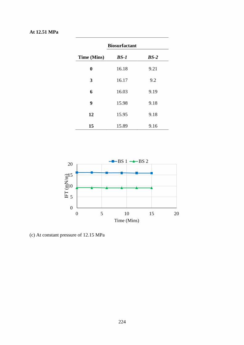
224

At 12.51 MPa

Biosurfactant


0 16.18 9.21

3 16.17 9.2

6 16.03 9.19

9 15.98 9.18

12 15.95 9.18

15 15.89 9.16


0

5

10

15

20

0 5 10 15 20

IFT

(m

N/m

)

Time (Mins)

BS 1 BS 2

225


At constant pressure of 0.15 MPa

Biosurfactant


0 12.63 6.69

3 12.51 6.60

6 12.42 6.55

9 12.19 6.50

12 11.77 6.41

15 11.64 6.37

0

5

10

15

20

0 5 10 15 20

IFT

(m

N/m

)

Time (Mins)

BS 1 BS 2

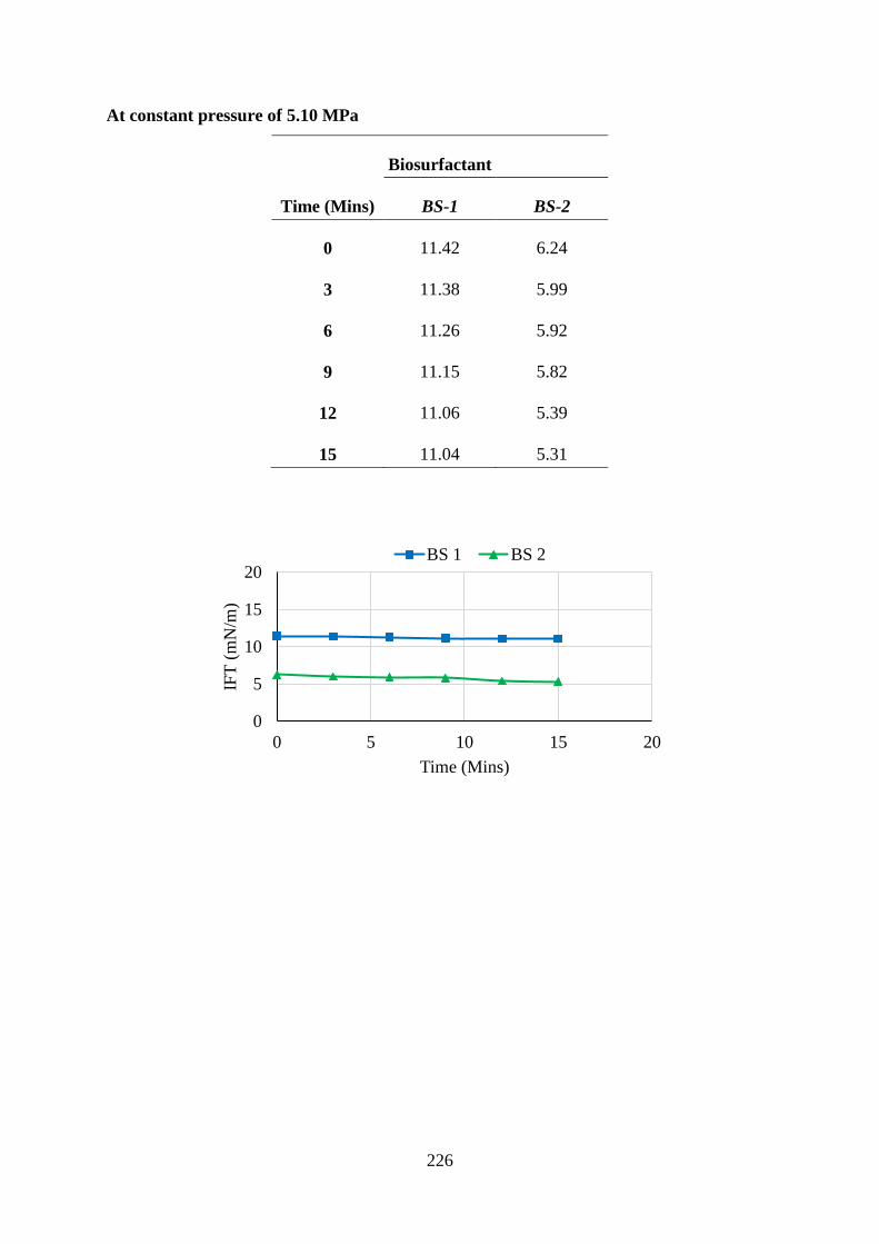
226

At constant pressure of 5.10 MPa

Biosurfactant


0 11.42 6.24

3 11.38 5.99

6 11.26 5.92

9 11.15 5.82

12 11.06 5.39

15 11.04 5.31

0

5

10

15

20

0 5 10 15 20

IFT

(m

N/m

)

Time (Mins)

BS 1 BS 2

investigation into the impact of biosurfactant in heavy oil...

Documents