INVERSION OF LIGHT SCATTERING MEASUREMENTS TO OBTAIN BIOGEOCHEMICAL PARAMETERS

J. Ronald V. Zaneveld1 (Presenter), Michael S. Twardowski2, Kusiel S. Shifrin1, W. Scott

Pegau1, Emmanuel Boss3, and Ilia Zolotov1 1Oregon State University, Ocean. Admin. Bldg 104, Corvallis, OR 97331

2WET Labs, Inc., Dept. of Research, 165 Dean Knauss Drive, Narragansett, RI 02882 3University of Maine, School of Marine Sciences, 5741 Libby Hall, Orono, ME 04469

INTRODUCTION

Renewed emphasis has been placed recently on the measurement of the volume scattering function, its moments, and its spectrum in natural waters. It is thus useful to review the methods of inversion of this data to obtain information regarding the nature of the particles. There is a very large literature on scattering inversions, so that this extended abstract cannot be complete. We have chosen to highlight a number of issues that could be addressed in the next few years using newly available instrumentation.

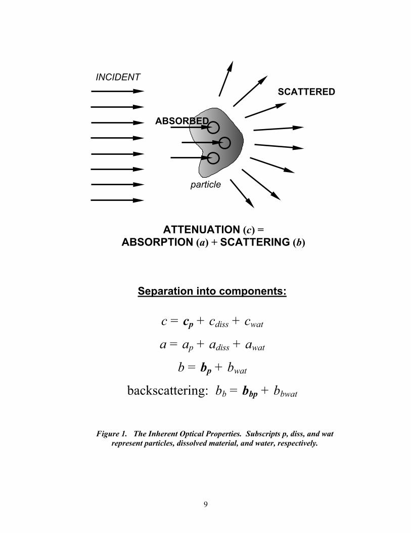
The interaction of an electromagnetic wave and a particle depends on the electromagnetic properties of the particle. For simple particles such as homogeneous spheres, these properties can be summarized by the size and complex index of refraction (m = n – in’). For more irregular particles, such as phytoplankton, in principle a complete description of the structure of the particle is necessary, that is internal complex index of refraction distribution and shape. Bulk measurements such as those obtained with light scattering, attenuation or absorption instrumentation linearly sum the properties of the individual particles if their concentration is not too high. It is obvious that inversion can at best reproduce the parameters that went into the original measurement. Therefore inversion of bulk inherent optical properties (IOP, Fig. 1; see also Mobley, 1994 for a review; see REFERENCES) cannot produce more than the parameters mentioned above. As will be further discussed below, researchers nonetheless have presented inversions to obtain Particulate Organic Carbon (POC), Total Suspended Mass (TSM), etc. The derivation of these parameters therefore depend on secondary (often empirical) relationships with the particulate size, shape, and index of refraction characteristics.

Inversion of light scattering by a collection of natural particles to obtain the details of all the particles is clearly not possible as the number of particulate parameters will always exceed the number of measured scattering parameters. Such an exact inversion is possible however, if the number of parameters is small. Polystyrene beads can be obtained commercially that have a very narrow, known size distribution and a known index of refraction. For a collection of this kind of particle nearly exact inversions are possible. The fact that that is possible is no guarantee that the same inversion method will be correct for mixtures of far more complex natural particles. THE FORWARD PROBLEM

Mie (1908) first gave the solution to Maxwell's equations for a plane electromagnetic wave interacting with a homogeneous sphere. In the past several decades, solutions have also been found for other shapes, such as cylinders, concentric

1

spheres, etc. In addition, T-matrix and other approximate methods allow the calculation of volume scattering functions for more complex particles (Mishchenko et al. 2000). An extremely useful approximation is the anomalous diffraction theory (Fig.2, Shifrin, 1988; van de Hulst, 1957). For an excellent library and commentary on the various forward solutions see the web site of Flatau (scatterlib section in http://atol.ucsd.edu/~pflatau/).

The IOP of natural particles can thus be approximated by means of theoretical calculations. It will always be necessary to estimate the size, shape, and m distribution of the particles that are assumed to contribute to the solution. The inversion will not be better than the errors induced by this estimation. The simpler the estimation, for example single parameter particle size distribution (PSD) and index of refraction, in general, the better the inversion converges to a solution. Such a convergence does not imply that the solution is correct. Multiple input parameters generally allow for a better match of measured and modeled optical parameters. Inversions using more parameters tend to have a shallow solution space, i.e., there are many possible solutions that minimize the difference between the measured and modeled parameters.

All methods of inversion therefore include a set of assumptions regarding the electromagnetic description of the particles. This is called regularization. We will discuss a number of solutions and look at how recent measurements and inversions fall within the overall scheme. For example, the usual assumption of homogeneous spheres and hyperbolic or Junge size distributions (Bader, 1970) allows one to obtain mathematical solutions from a number of optical measurements, such as forward light scattering, the ratio of the back scattering to total scattering, and the light scattering spectrum. The accuracy of the solution then depends on the accuracy of the regularization assumptions. We will discuss a number of recent approaches to inversion and discuss their accuracy in light of recent calculations of scattering by inhomogeneous and non-spherical particles. ONE PARAMETER INVERSIONS

Inversions for a single parameter imply that the other parameters are known or are assumed to not contribute to the solution. Clearly such simple inversions deal with the assumption of a single parameter size distribution and a single index of refraction for the collection of particles. We will start with inversions for the size distribution.

Shifrin (1988) describes the method of small angles. Small angle scattering is dominated by diffraction. Diffraction by large particles (d / λ>>1, i.e. the particles are much larger than the wavelength of light) into small angles is independent of n. Therefore, the size distribution of the larger particles can be inverted from knowledge of the small angle scattering. Since oceanic particle collections typically contain large concentrations of particles d and λ are nearly equal, the small angle method is only applicable in oceanic settings for the derivation of the PSD of the large particle fraction.

Another inversion is based on the potentially simple connection between the slope of the PSD and the shape of the beam attenuation spectrum (a recent analysis is given in Boss et al., 2001). Forward models for the inversion are based on Junge size distributions and a single index of refraction. Fig. 3 shows results of Mie theory calculations for this relationship. The relationship depends on the limits of integration for the particle size. In the ocean this relationship was first evaluated observationally by Kitchen et al. (1982), who showed that the slope of the beam attenuation spectrum (including CDOM) was not

2

highly correlated with chlorophyll to total suspended volume ratios (a proxy for the index of refraction), but was correlated with the slope of the size distribution. Closure between the in-situ beam attenuation spectrum and Coulter measurements of PSD of discrete water samples was obtained by Boss et al. (2001). Most recently, Oubelkheir (2002) showed that patterns of the slope of the PSD and c(λ) showed similar diel patterns. This relationship deserves further investigation. Errors due to the size distribution not being Junge shaped and inhomogeneous particles must be evaluated.

If one were to assume that the PSD was known, either by independent measurement or from c(λ), then in the simple inversion, the only unknown is the index of refraction. PSDs can be determined approximately from a number of devices. The most prevalent is the Coulter Counter, which measures the change in resistivity when a particle passes through a narrow orifice in an electric field. Such devices were used extensively in the past (Brown and Gordon,1974; Kitchen et al,1978) and continue to be used. From the equations in Fig. 2, it can be deduced that if the size distribution is known (or assumed), n can be determined by iteration. Brown and Gordon (1974) and Bricaud et al. (1983) describe examples of this approach. Iteration using Mie theory or anomalous diffraction has the advantage that an actual measured size distribution can be used. The only error then comes from the assumption that the particles are homogeneous and all have the same index of refraction. In addition, Bricaud et al. (1983) looked at cultures with narrow size distributions. The iterative approach is particularly well suited to this situation as potential errors in the size distribution do not propagate into the determination of n. If the PSD is obtained from inversion of c(λ), a further error is introduced. The latter approach is a two parameter inversion described below.

Shifrin (1988) describes the method of fluctuations. In this method it is assumed that there are few enough particles in the beam of a beam transmissometer to cause statistical fluctuations in the transmitted light. Because of this requirement the method applies primarily to large particles. The method gives the mean size and concentration of these particles. The smaller particles are present in large enough numbers so that their signal is a steady background. It would thus, in theory be possible to get the size distribution of the smaller particles from the attenuation spectrum and the size distribution of the larger particles from the temporal fluctuations of the signal. As far as we know this has not yet been done.

The real part of the index of refraction can also be determined directly by immersion (Bryant et al. 1969, cited in Bricaud and Morel, 1986). In this method, the index of the suspending fluid of the particles is varied until a minimum in the light scattering is observed. Morel points out that this leads to an n dominated by the outer shell, which is not the average n of the entire particle. On the other hand this n may be the one that is appropriate for scattering calculations. TWO PARAMETER INVERSIONS

One can define the optical properties of collections of particles using only two parameters. This is done by using Mie theory for homogeneous spheres, and assuming a one parameter particle size distribution such as the Junge distribution. The two parameters are then the slope of the Junge distribution and the m of the particles. If the particles are assumed to be non-absorbing (n’ = 0), the problem is further simplified. We

3

will leave till later the question as to how correct the assumptions are. With these two parameters one can then calculate all VSF characteristics. It is then possible to invert two VSF related parameters to get the Junge slope and index of refraction. It is advantageous to find two VSF parameters that are nearly orthogonal, that is, one is largely a function of the index of refraction, and the other is largely a function of the Junge slope.

Morel (1973) used Mie theory to examine a number of parameters. Morel (1973) showed two parameter plots for β(4°)/b, β(6°)/b, β(44°)/b, and β(90°)/b (Fig. 4). These show the gradual transition from the dominant dependence of the forward scattering on the Junge slope, to the larger influence of n for the larger angles. Based on this it stands to reason to use a combination of forward scattering and backward scattering to obtain the two particle parameters. These included various β(θ)/b as well as β(θ1)/β(θ2). Morel chose β(10°)/β(2°) to be indicative of the near-forward shape of the VSF and β(140°)/β(10°) for the larger angle shape of the VSF (Fig. 5). Morel showed that the β(140°)/β(10°) ratio is more dependent on the index of refraction and β(10°)/β(2°) is more dependent on the Junge slope for lower indices of refraction. He then used measurements of these parameters from various locations to determine bounds on the range of Junge slopes and n that could be found in the ocean regions examined (Fig. 6). By using ratios of values of the VSF, it is not necessary to obtain absolute calibration of the meter. With the advent of new VSF meters this approach should be re-examined.

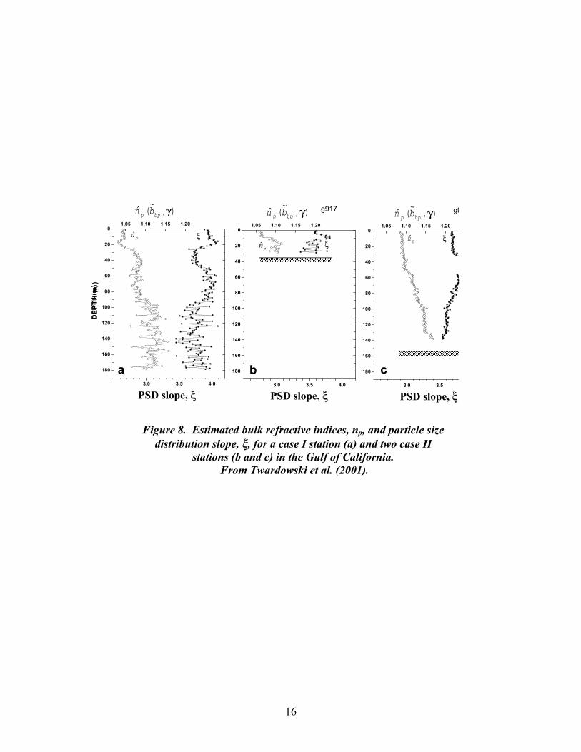
Nearly thirty years later, Twardowski et al. (2001) used a similar approach to obtain the same particle parameters. The parameters used are the slope of the attenuation

spectrum γ and the ratio of the backscattering coefficient to total scattering, ~ bbp. The slope of the attenuation spectrum is a proxy for the Junge slope of the PSD (see above). The curves obtained from Mie theory together with data from the Gulf of California are shown in Fig. 7. Profiles of particulate parameters obtained from optical measurements are shown in Fig. 8. It is interesting to note that while Morel estimates values for ξ (m in Figs. 4 and 5) from 3.8 to 4.4, Twardowski et al. estimate values for ξ from 3.5 to 4. This difference may reflect different influences from different size particles with the two methods. Morel obtains a range for the real part of the index of refraction from 1.03 to 1.06 in waters predominantly case I, while Twardowski et al. obtain values ranging from 1.04 to 1.18 in both case I and case II waters (Figs. 7, 8). It will be interesting to use complete experimental data sets including the PSD for validation to study these differences in derived values.

Two parameter inversions can also be carried out using flow cytometers (Ackleson and Spinrad, 1988; Green, 2002). Flow cytometers measure two scattering parameters with broad angular subtends; one in the forward direction and one sideways. Flow cytometers measure individual particles. If the weighting functions of such measurements can be accurately determined, inversions for the size and index of the individual particles can be determined. MULTIPLE PARAMETER INVERSIONS

This method was called the fitting method by Shifrin (1988). In this method, one fits the VSF over as large a range of angles as possible. As discussed before in the small angle approximation, the small angles fit should provide information on the large particles, and the large angles provide information on the smaller particles. Typically one

4

varies size distributions and indices until a reasonable fit to experimental data is obtained (Kullenberg, 1970; Brown and Gordon, 1974). A systematic approach was described by Zaneveld et al. (1974). They used Mie theory to obtain VSFs for five n and eight Junge slopes. They used a minimization scheme to obtain the best fit to VSF data obtained by Kullenberg (1970). It was found that usually the best fit to experimental data was obtained by a combination of particles consisting of a low n component (1.02 or 1.05) with a small Junge slope (3.1 to 3.3) and a component with an n of 1.15 and Junge slopes of 4.4 to 5.0. This unsurprising result indicates that large, low index, organic particles mostly determine the forward scattering, and small inorganic or detrital particles with high indices determine the scattering at larger angles. Clearly this kind of inversion can be no better than the accuracy of the components. There is no certainty that components of the type assumed actually exist. However these methods show that single index, single Junge slope models cannot give as good a fit to the VSF as more complex models.

More complicated methods such as that given by Shifrin and Zolotov (1997) use an iterative method for inverting simultaneous data for the aerosol spectral attenuation and small-angle phase function into the aerosol particle size distribution (APSD). This method is applicable to oceanic situations as well. The inversion of the small-angle phase function could not be applied directly to the whole system, because the presence of small particles distorted the picture of the small-angle scattering. Recourse was made to an iterative procedure. The smaller-sized APSD was determined from inverting the aerosol spectral attenuation coefficient. The phase function for this part was calculated and eliminated from the total phase function, after which the large-particle part of APSD was determined by inversion. The procedure was repeated until the desired accuracy was achieved. It was shown that, given certain conditions, this inversion method was capable of retrieving an APSD for a radius interval of 0.2-30 µm with a mean relative error of less than 10 % and a maximum deviation not exceeding 20 %.

A novel approach to inversion of VSFs is given in Shifrin and Zolotov (2002a,b,c). The method of mean ordinates was developed for inverting scarce or incomplete light scattering data, such as lidar observations of attenuation and/or backscattering at one or two wavelengths. In inversion methods where look-up tables are used, the criterion for choosing the solution is the closeness of a model to the measured value. In case of low-accuracy data, this can result in gross inversion errors. Based on a priori information of atmospheric aerosols in a given region, the parameterization of APSD was performed and the limits of aerosol parameter variations were established. All possible parameter combinations were used for constructing aerosol models for which attenuation and backscattering coefficients were calculated. The models that yielded the extinction and backscattering coinciding, within preset limits, with those obtained from experiment were considered as acceptable solutions. The mean over all acceptable solutions was calculated. The acceptable solution found to be the closest to this mean was considered as the most probable solution to the problem of inverting lidar data into APSD. The method of mean ordinates was tested in many numerical experiments and by using experimental data obtained in the Shoreline Environment Aerosol Studies 2000. The method proved its feasibility of ensuring the retrieval accuracy comparable to that of direct APSD measurements.

In nearly all inversion models cited above, Mie theory or anomalous diffraction of homogeneous spheres is used to develop models of collections of particles. Recently,

5

some studies have been carried out on light scattering by collections of spheroids (Herring, 2002; MacCallum, 2002). These studies show that compared to spheres with equal volumes, spheroids have maximum scattering deviations of about 30%. For a collection of spheroids the deviation will be smaller. Scattering by three layered spheres (Kitchen and Zaneveld, 1992, 1995) is difficult to compare to homogeneous spheres, as one cannot easily assign an "average" index of refraction. An average index by volume makes most sense biologically, but optically the outer shell, especially if it is hard, may dominate. It can be said in general that high index outer shells make particles scatter more like high index particles. The optical average index will thus not equal the volumetric average index. Inversion will produce a value closer to the optical average, as this is what causes the similarity in light scattering features.

Since it takes six parameters to describe the structure of a three layered sphere, inversion for a collection of such spheres is not likely. The effect of inversion using incorrect models is difficult to assess in general terms, as scattering by inhomogeneous non-spherical particles can be larger or smaller than spheres of equal volume and volume average index. Errors in scattering models will manifest themselves upon inversion as errors in size distributions and average indices of refraction. Inversions of natural particle collections will thus always remain quasi-qualitative. It has been long recognized however (Parsons, 1969), that even approximate information on particles can be extremely useful in understanding community structure. Such information has also been used to study particle dynamics (Boss et al., 2001; Twardowski et al., 2001). BIOGEOCHEMICAL PARAMETERS

If the nature of the particles (i.e., size, shape, and internal m distribution) is approximately constant, the total number of particles becomes proportional to scattering at any angle, provided multiple scattering does not occur. Parameters such as TSM and POC are then proportional to the scattering observation. POC is often cited as being correlated with scattering or attenuation measurements (e.g., Bishop, 1999; Mishonov et al., 2000) and with reflectance measurements (Stramski et al., 1999). Clearly this dependence is primarily a function of particle concentration and secondarily a function of the size and index of the particles. Without further specific information, the slope of correlations of POC and c can be attributed to either PSD changes or index changes. The slope of the correlation is determined by the nature of the particles. Examples are shown in Figs. 9 for TSM and Figs. 10 and 11 for POC.

We have briefly (and by no means exhaustively) described above a number of approaches toward inversion of VSF data. The methods all have in common that the best one can achieve is to obtain the PSD and bulk n. These parameters alone can say much about the nature of the particles. Size, while seemingly an obvious parameter, becomes far more difficult to define for non-spherical objects. Particle volume is more clearly defined and this is measured by resistive pulse counters. Even volume becomes more difficult to define for particle aggregates. The response of resistive pulse counters to aggregates that contain large proportions of water is difficult to predict. Nonetheless, much can be potentially learned from the inversions. What is needed is a renewed emphasis on validation of the inversions.

6

REFERENCES 1. Ackleson, S.G. and R.W. Spinrad, 1988, Size and refractive index of individual

marine particulates: a flow cytometric approach, Appl. Opt. 27, 1270-1277.

2. Bader, H., (1970), The hyperbolic distribution of particle sizes. J. Geophys. Res. 75: 2823- 2830.

3. Bishop, (1999), Spatial and temporal variability of POC in the northeast Subarctic Pacific, Deep Sea Res. II, 2699-2733.

4. Boss et al., (2001), Spectral particulate attenuation and particle size distribution in the bottom boundary layer of a continental shelf. J. Geophys Res. 106, 9499-9508.

5. Boss et al., (2001), Shape of the particulate beam attenuation spectrum and its inversion to obtain the shape of the particulate size distribution. Appl. Opt., 40:4885-4893.

6. Bricaud, A., Morel, A., and L. Prieur, (1983), Optical efficiency factors of some phytoplankters, Limnology and Oceanography, 28, 816-832.

7. Bricaud and Morel, (1986), Light attenuation and scattering by phytoplankton cells: a theoretical modeling, Appl. Opt. 25, 571-580.

8. Brown, O.B. and H.R. Gordon, (1974), Size-refractive index distribution of clear coastal water particulates from light scattering. Appl. Optics 13, 2874- 2881.

9. Green, R., (2002) Scale closure in upper ocean optical properties: from single particles to ocean color. Ph.D. thesis, WHOI/MIT, 168 pp.

10. Herring, S. 2002. A Systematic Survey of the Modeled Optical Properties of Nonspherical Marine-Like Particles, MSc. Thesis, Oregon State University, 43pp.

11. Kitchen, J. et al., (1978), The vertical structure and size distributions of suspended particles off Oregon during the upwelling season. Deep-Sea Res. 25: 453-468.

12. Kitchen, J. et al., (1982), Effect of particle size distribution and chlorophyll content on beam attenuation spectra. Appl. Opt. 21: 3913-3918.

13. Kitchen, J. and R. Zaneveld, (1992), A three-layered sphere model of the optical properties of phytoplankton. Limnol. Oceanogr , 37, 1680-1690.

14. Kullenberg,G., (1970), A comparison between observed and computed light scattering functions II. Univ. of Copenhagen Report No. 19, 15pp.

15. MacCallum, I. , (2000), Measurement and modeling of phytoplankton light scattering, Ph.D. thesis, University of Strathclyde, Glasgow, 228 pp.

16. Mie, G., (1908), Ann. Physik, 25, 377.

17. Mishchenko (Ed.) et al., (2000), Light scattering by nonspherical particles, 690pp.

18. Mishonov, W.D. Gardner, M.J. Richardson. (2000), Global POC Synthesis from Beam Attenuation Data collected during JGOFS, WOCE and other programs, JGOFS-SMP PI's workshop at WHOI (Clark), July 10-15. see http://oceanography.tamu.edu/%7Epdgroup/TAMU-SMP.html.

7

19. Mobley, C., (1994), Light and Water, 592 pp.

20. Morel, (1973), Diffusion de la lumière par les eaux de mer; résultats expérimentaux et approche théorique, in AGARD Lect. Ser., pp. 3.1.1.-3.1.76

21. Obelkheir, K., (2001), Caractérisation biogéochimique de provinces océaniques à l'aide d'indicateurs bio-optiques, à diverses échelles spatio-temporelles, Ph.D. thesis, L’Universite de la Mediterranee, 372 pp.

22. Parsons, T.R., (1969), The use of particle size spectra in determining the structure of a plankton community. J. Oceanog. Soc. Japan. 25: 6-15.

23. Peterson, 1977. Ph.D. thesis, Oregon State University.

24. Shifrin, K.S., (1988), Physical optics of ocean water, 285 pp.

25. Shifrin, K.S. and I.G. Zolotov, (1997), Determination of the aerosol particle size distribution from simultaneous data on spectral attenuation and the small-angle phase function. Appl. Optics, 36, 6047-6056.

26. Shifrin, K.S. and I.G. Zolotov, (2002), The Use of Direct Observations Over the Aerosol Particle Size Distribution for Inverting Lidar Data, submitted in J. Atmos. Ocean. Tech.

27. Shifrin, K.S. and I.G. Zolotov, (2002), A method for retrieving the aerosol particle size distribution in the marine atmospheric boundary layer from horizontal lidar data.

28. Shifrin, K.S. and I.G. Zolotov, (2002), An inversion method for scarce lightscattering data, poster at Ocean Optics XVI.

29. Twardowski et al., (2001), A model for estimating bulk refractive index from the optical backscattering ratio and the implications for understanding particle composition in Case I and Case II waters. J. Geophys. Res., 106(C7):14,129-14,142.

30. van de Hulst, (1957), Light scattering by small particles, pp. 470.

31. Zaneveld et al., (1974), The determination of the index of refraction distribution of oceanic particulates. J. Geophys. Res. 79(27): 4091-4095.

32. J.R.V.Zaneveld and J.C.Kitchen, (1995), The variation in the inherent optical properties of phytoplankton near an absorption peak as determined by various models of cell structure. J.Geophys Res. 100(C7), 13,309-13,320.

33. Zaneveld, J.R.V. and H. Pak, (1973), A method for the determination of the index of refraction of particles suspended in the ocean. J. Opt. Soc. Am. 63(3): 321-324.

8

SCATTERED

ABSORBED

INCIDENT

ATTEABSORPTION

Separatio

c = c

a = a

b

backscatter

Figure 1. The Inherent Oprepresent particles, diss

particle

NUATION (c) = (a) + SCATTERING (b)

n into components:

p + cdiss + cwat

p + adiss + awat

= bp + bwat

ing: bb = bbp + bbwat

tical Properties. Subscripts p, diss, and wat olved material, and water, respectively.

9

Figure 2. Equations and plot of the attenuation, absorption, and scattering efficiencies

(Qc, Qa, and Qb) as predicted from the van de Hulst (1957) anomalous diffraction approximation of Mie theory. The parameter ρ = 2πd(n-1) / λw, and ζ = n’/(n-1), where d is sphere diameter and n and n’ are the real and imaginary parts of the complex refractive index. Thus, the efficiencies for a homogeneous sphere are a

function of particle diameter, complex refractive index, and wavelength only. Bulk

particle attenuation is proportional to the efficiency of each particle, c .

Figure reproduced from Morel and Bricaud (1986).

∑=

∝N

iiip dQ

1

2

10

n’ = 0

Figure 3. Relationship between the hyperbolic slope of the particle size distribution and the slope of cp. Computed from Mie theory with fixed

size limits to the particle distribution. When particles absorb, deviations from model occur for ξ > 4. Adapted from Boss et al. (2001).

11

Figure 4. The volume scattering coefficient, β, evaluated at 4 angles and normalized to total scattering, b, as function of refractive index, n, and the hyperbolic slope of the particle size distribution, m. Based on Mie theory.

Reproduced from Morel (1973).

12

Figure 5. Two ratios of the volume scattering coefficient as function of refractive index, n, and the hyperbolic slope of the particle size distribution, m. Same values used

as in the previous figure. Based on Mie theory. Bracketed ranges match range in values obtained by experimental observations in case I waters. Reproduced from

Morel (1973).

13

Figure 6. Representation of the region of bulk refractive indices and PSD slopes (“exposant”) that satisfy experimental scattering ratio measurements, adapted from Fig. 5. The range in PSD slopes reflects measurements of the shape of near forward

scattering, i.e., β(10°)/β(2°), and the range of indices reflects measurements of the ratio of backscattering to forward scattering, i.e., β(140°)/β(10°).

Reproduced from Morel (1973).

14

Figure 7. Estimated bulk refractive indices from four regions of the Gulf of California: Ic – Case I, chlorophyll maximum; Id – Case I, deep water; IIa – Case II,

south of midrift islands; and IId – Case II, bottom water, north of midrift islands. Model is based on Mie theory, assuming an n’=0.005. Refractive index contours range

from 1.02 to 1.20 in 0.02 increments. Adapted from Twardowski et al. (2001).

15

180

160

140

120

100

80

60

40

20

0

3.0 3.5

3-s

3 - s ( ≈ ξ )

1.05 1.10 1.15 1.20

180

160

140

120

100

80

60

40

20

0

3.0 3.5 4.0

3-s

g917

3 - s ( ≈ ξ )

DEP

TH (m

)

1.05 1.10 1.15 1.20

180

160

140

120

100

80

60

40

20

0

3.0 3.5 4.0

3-s

g9

3 - s ( ≈ ξ )

1.05 1.10 1.15 1.20

������������������������������������������������������������������������������������������������������������������������������������������������������������������������������������������������������������������������������������������������������������������������������������������������������������������������������������������������������������������������������������������������������������������������������������������������������������������������������������

���������������������������������������������������������������������������������������������������������������������������������������������������������������������������������������������������������������������������������������������������������������������������������������������������������������������������������������������������������������������������������������������������������

a b c

ξ ξ

ξ

PSD slope, ξ PSD slope, ξ PSD slope, ξ

),~(ˆ γbpp bn

pn̂ pn̂

pn̂

DE

PTH

(m)

),~(ˆ γbpp bn),

~(ˆ γbpp bn

Figure 8. Estimated bulk refractive indices, np, and particle size distribution slope, ξ, for a case I station (a) and two case II

stations (b and c) in the Gulf of California. From Twardowski et al. (2001).

16

c (m-1)

c (m-1)

c (m-1)

TSM (µg L-1)

Figure 9. Beam attenuation vs. total suspended matter concentration (TSM) for different water types off the Oregon shelf.

From Peterson (1977).

17

0

0.5

1

1.5

2

2.5

3

0 40 80 120 160

Ross SeaNABEAPFZLinear (Ross Sea)Linear (NABE)Linear (APFZ)

PPOOCC,, µµMM CC//LL

ccpp ((mm--11))

(PR

Figure 10. Relationship between cp and particulate organic carbon OC) from Mishonov et al. (2000). Regressions are y=0.0178x - 0.0155 2=0.874 for the Ross Sea, y=0.0376x - 0.0032 R2=0.913 for the North Atlantic Bight Experiment, and y=0.0264x - 0.0649 R2=0.982 for the

Antarctic Polar Front Zone.

18

Figure 11. Relationship between c and particulate organic carbon (POC) from Bishop et al. (1999). Data from 1996 and

1997 C-JGOFS.

19