1

Inversion and sensitivity analysis of

Ground Penetrating Radar data with

waveguide dispersion using deterministic

and Markov Chain Monte Carlo methods

Jutta Bikowski (j.bikowski@fz-juelich.de), Johan A. Huisman, Jasper A. Vrugt, Harry

Vereecken, and Jan van der Kruk

Abstract

Ground Penetrating Radar (GPR) has found widespread application for the non-invasive

characterization of the subsurface. Nevertheless, the interpretation of GPR measurements remains

difficult in some cases, particularly when the subsurface contains thin horizontal layers with

contrasting dielectric properties that might act as waveguides for electromagnetic wave

propagation. GPR data affected by waveguide dispersion are typically interpreted using the so-

called dispersion curve, which describes the phase velocity as a function of frequency. These

dispersion curves are commonly analyzed with deterministic optimization algorithms and which

return dielectric properties of the subsurface as well as the location and depth of the respective soil

layers. Unfortunately, current state-of-the-art- inversion methods do not provide estimates of the

associated uncertainty of the inferred subsurface properties. Here, we apply a Bayesian inversion

methodology using the recently developed DiffeRential Evolution Adaptive Metropolis DREAM(ZS)

algorithm. This Markov Chain Monte Carlo simulation method is admirably suited to estimate

(nonlinear) parameter uncertainty and treat measurement error explicitly. Analysis of synthetic

GPR data showed that the frequency range used in the inversion has an important influence on the

estimated values of the parameters. This is related to the parameter sensitivity that varies with

frequency. Our results also demonstrate that measurement errors of the dispersion curve are

frequency dependent, and that the estimated model parameters become severely biased if this error

is not properly treated. We demonstrate how frequency dependent measurement errors can be

estimated jointly with the model parameters using the DREAM(ZS) algorithm. The posterior

distribution of the model parameters derived this way compared well with inversion results for a

reduced frequency bandwidth which is another method to reduce the bias introduce through

measurement error. Altogether, the inversion procedure presented herein provides an objective

methodology for analysis of dispersive GPR data, and appropriately treats measurement error and

2

parameter uncertainty. The full frequency bandwidth is deliberately used to reduce the need for

subjective decisions regarding which frequencies to use in the inversion.

Keywords:

GPR, Inversion, Monte Carlo Markov Chain, Dispersive data, Measurement error, Uncertainty

Introduction

Ground penetrating radar (GPR) is a geophysical technique that emits electromagnetic waves

into the soil using a transmitter antenna, and measures the intensity of the electrical field at

receiver antenna(s) as a function of time. Typically, the transmitting and receiving antennas are

placed on the ground (i.e. on-ground GPR). The waves that are transmitted into the soil will be

partly reflected and partly transmitted when contrasts in dielectric permittivity associated with

subsurface structures occur. The propagation velocity of the GPR waves depends on the

dielectric permittivity, which in turn can be related to soil moisture content and soil porosity

amongst other factors.

GPR is widely used in many research fields, including civil and environmental engineering,

archeology, pavement and infrastructure characterization, mining, and extraterrestrial

exploration. In recent years, GPR has especially found widespread use in the field of

hydrogeophysics because of its ability to non-invasively monitor and map soil water content and

to characterize the near-surface structures controlling hydrological processes (e.g. van

Overmeeren et al. 1997; Huisman et al. 2001; Galagedara et al. 2003, Huisman et al. 2003a,

Moysey 2004, Bradford 2008, Westermann et al. 2010; Haarder et al. 2011; Rhim 2011;

Steelman and Endres 2011). Both subsurface characterization and soil water content

determination using GPR rely on an accurate determination of the propagation velocity of GPR

waves. For on-ground GPR, this propagation velocity and therewith the dielectric permittivity

can be determined when GPR measurements are made with multiple offsets between the

antennas, for example using a common midpoint (CMP) measurement where the antenna

separation is increased while keeping the same midpoint. In such a CMP measurement, reflected

GPR waves can be identified by their hyperbolic shape that can be used to estimate the depth of

the reflecting layer and the average propagation velocity of the subsurface above the reflecting

layer (Greaves et al. 1996; van Overmeeren et al. 1997; Dannowski and Yaramanci, 1999;

Endres et al., 2000; Bohidar and Hermance, 2002; Garambois et al., 2002, Grote et al., 2003;

Lunt et al., 2005; Turesson A. 2006; Gerhards et al., 2008). Another wave that has been used for

soil water content determination is the ground wave, which is the direct transmission from sender

3

to receiver antenna through the top of the soil. The ground wave can be recognized in a CMP

measurement by the linear increase in arrival time with antenna separation, and the ground wave

propagation velocity can be easily determined from the slope of this increase. The ground wave

velocity has been widely used to measure the spatio-temporal development of soil water content

variability (e.g. Galagedara et al. 2003; Huisman et al. 2003b; Weihermüller et al., 2007).

Although the use of the ground wave is a promising method for soil water content

measurements, difficulties arise when the subsurface exhibits strong vertical variability due to the

presence of distinct soil layers or gradients in soil moisture content that introduce thin horizontal

layers with a strong contrast in dielectric permittivity. If the depth of the layers are comparable to

or smaller than the wavelength of the GPR signal, these layers can act as a waveguide in which

the electromagnetic waves are trapped. This leads to positive interference related to total

reflection of the trapped wave at the boundaries of the layer. Field situations where such

waveguides have been reported include a thin ice sheet floating on water (Arcone 1984; van der

Kruk et al., 2007), a water infiltration front in a dry soil (Arcone et al. 2003), a thin organic-rich

sandy silt layer overlying a gravel unit (van der Kruk et al. 2006), a mountain slope with a 1 m

soil cover (Strobbia and Cassiani, 2007), and thawing of a frozen soil layer (van der Kruk et al.,

2009; Steelman et al., 2010). In the presence of such waveguides, CMP measurements are

difficult to interpret because the arrival time and the first cycle amplitude of the ground wave

cannot be identified due to interfering waves.

In order to enable interpretation of GPR data with waveguide dispersion, van der Kruk et al.

(2006) presented a deterministic inversion algorithm to estimate the thickness and permittivity of

the dispersive waveguide and the permittivity of the soil below the waveguide. This work drew

inspiration from inversion algorithms that are used to interpret dispersive Rayleigh and Love

waves commonly observed in multi-offset seismic data. The deterministic inversion method of

van der Kruk et al. (2006) was later extended for higher order modes by van der Kruk (2006) and

van der Kruk et al. (2007). More recent extensions now enable inversion for the case that

multiple layers act as waveguides (van der Kruk et al. 2010).

Inversion of GPR data affected by waveguide dispersion requires a forward model that

accurately describes the dispersive characteristics of GPR data for a given subsurface structure

described by a set of model parameters. Optimization methods are then used to seek a set of

model parameters that minimizes the discrepancy between simulated and measured GPR data.

Because such an inversion is nonlinear and ill-posed, a unique ‘best’ model might not exist or

might be hard to find. In general, numerical modeling and inversion methods for GPR data have

been greatly improved in the last decade, which obviously enhances the quality of inversion

4

results as well as the range of GPR data that can be inverted. Yet, traditional GPR inversion

algorithms are deterministic, and estimate only a single ‘best’ set of model parameters without

consideration of parameter uncertainty (e.g. Pettinelli et al. 2007; Steelman and Endres 2010;

Wollschläger et al. 2010). Therefore, it is not yet well established how errors in GPR

measurements and models propagate through the processing and inversion of dispersive GPR

data. For non dispersive data, confidence intervals of the wave velocity and hence implicitly of

the electrical permittivity have been reported which vary widely depending on the field settings

and methods used (e.g. Jacob and Hermance 2004). Typical sources of error in GPR

measurements introduced during GPR data acquisition are inaccuracies in offset, timing, antenna

orientation, and other antenna effects (Slob 2010). An additional error source that is more

complicated to address is model structural uncertainty, which is introduced by the use of

simplifying assumptions in the modeling of GPR data.

Clearly, it is desirable to simultaneously estimate the ‘best’ model parameters and their

associated uncertainty. Bayesian inversion algorithms based on Markov Chain Monte Carlo

(MCMC) methods are particularly well suited for this task. MCMC methods use random walks

through the parameter space to sample the joint posterior probability distribution of the model

parameters that describes parameter uncertainty. MCMC methods are not new in the field of

geophysical inversion (Mosegaard and Tarantola, 1995; Sambridge and Mosegaard, 2002), but

the ever increasing computational power has resulted in their increased use in recent years,

especially in the field of hydrogeophysics (e.g. Strobbia and Cassiani 2007; Irving and Singha,

2010; Hinnell et al. 2010; Huisman et al. 2010).

In this study, we invert synthetic and experimental GPR data with waveguide dispersion and

determine the posterior model parameter distribution using a state-of-the-art MCMC algorithm.

This posterior probability density function is used to investigate parameter uncertainty and

sensitivity. In particular, we show that the posterior parameter estimates are sensitive to the

frequency bandwidth of the data used in the inversion and that the measurement error is

frequency dependent. To provide stable parameter estimates, we introduce a novel MCMC

framework that simultaneously infers the model parameters and the frequency dependent

measurement error.

The remaining part of this paper is organized as follows. We first describe the deterministic

and MCMC inversion methods. Then, a synthetic case study is used to illustrate the effects of

frequency bandwidth selection and measurement error on the final parameter estimates. Next, a

real-world GPR data set is analyzed and used to demonstrate how model parameters and

5

measurement errors can be jointly retrieved from the measured dispersion curve. Finally, the last

section of this paper summarizes our main results and provides some conclusions.

Methodology

The general flow of our deterministic and Bayesian inversion strategies is summarized in

Figure 1. First, the CMP data, E(x,t), depending on the offset, x, of the antennas and time t, are

processed to obtain a so-called dispersion curve (Park et al. 1998; van der Kruk 2006). The first

processing step is to transform E(x,t) into the frequency domain, ),(ˆ fxE , with a Fourier

transformation. Then, the phase-velocity spectrum is calculated by:

xv

fi

fxE

fxEfvD

x

2exp

),(ˆ

),(ˆ),(

[1]

where v is the phase velocity, f is frequency and i is the square root of -1. In the final processing

step, the dispersion curve, vmeas

(f), is obtained by selecting the phase velocity with maximum

amplitude for each frequency. This dispersion curve constitutes the measured data in the

following deterministic and Bayesian inversion strategies.

The forward model to simulate a dispersion curve is based on modal theory (Budden 1961; van

der Kruk, 2006). It assumes that the waveguide consists of a single high permittivity layer

overlying a halfspace with lower permittivity (Figure 2). The model parameters of the single

layer model are the dielectric permittivity and height of the waveguide ( 1 and h) and the

permittivity of the halfspace ( 2). The highest phase velocity of a single-layer guided wave is

given by 20 /c , where c0 denotes the speed of light (van der Kruk 2006; van der Kruk et al.

2006). It is obtained for low frequencies because the dispersion curve decreases monotonically

with frequency. A first rough estimate of 2 can thus be calculated from the highest measured

phase velocity. This also suggests that an adequate representation of low frequencies is required

to obtain accurate estimates of ε2. For high frequencies, the phase velocity approaches an

asymptote given by 10 /c , which similarly suggests that an adequate representation of high

frequencies is required for accurate estimates of ε1. However, the direct estimation of 1 and 2

from the dispersion curve can be difficult because of the low signal to noise ratio for low and

high frequencies.

6

Inversion algorithms

Two inversion algorithms are used in this study: the deterministic inversion algorithm

presented in van der Kruk et al. (2006) and the DiffeRential Evolution Adaptive Metropolis

(DREAM(zs)) algorithm presented in Vrugt et al. (2009).

Deterministic inversion

The deterministic inversion approach of van der Kruk (2006) aims to find the model

parameters (m= ε1, ε2, h) that minimize the difference between modeled and measured

dispersion curves. In contrast to van der Kruk et al. (2006), we minimize the mean squared

difference between modeled and measured dispersion curves (L2 norm). In the first step of the

deterministic inversion approach, the feasible parameter space is sampled using a regular grid.

In the second step, each of these parameter combinations is used as a starting value for a local

search using the Simplex method (Lagarias et al. 1998). The model parameters with the smallest

misfit are assumed to represent the best possible subsurface model describing the dispersive

GPR data. Application of this inversion algorithm to synthetic and measured dispersive GPR

data showed robust and reliable results (van der Kruk 2006; van der Kruk et al. 2006; van der

Kruk et al. 2007; van der Kruk et al. 2010).

Markov Chain Monte Carlo Simulation: The DREAM(ZS) algorithm

MCMC algorithms have found widespread application and are used to estimate the most

likely values of model parameters along with their posterior probability distribution. This

posterior probability distribution contains all the necessary information to estimate parameter

uncertainty and sensitivity. Unfortunately, standard MCMC algorithms are generally inefficient,

and even very simple problems typically require many thousands of model evaluations to

converge to the posterior probability distribution. This work capitalizes on recent developments

in MCMC simulation and uses the DiffeRential Evolution Adaptive Metropolis (DREAM(ZS))

algorithm (Vrugt et al. 2009). The algorithm runs multiple Markov chains (random walk

trajectories) in parallel, and maintains detailed balance and ergodicity. Whereas standard

MCMC algorithms require extensive tuning, DREAM(ZS) automatically scales the orientation

and scale of the proposal distribution during sampling. This proposal distribution is used to

generate new points in each Markov chain. The only information to be specified by the user is

the parameter ranges, and the likelihood function to compare model predictions with respective

observations. A detailed description of the algorithm can be found in Vrugt et al. (2009), and is

beyond the scope of the current paper.

Many likelihood functions have been developed in the literature, and these functions differ in

their underlying treatment of the error residuals. We adopt a relatively simple likelihood

7

function, L(m |vmeas

) that assumes that the residuals between modeled and measured dispersion

curve are normally distributed and mutually independent:

K

k k

me

k

meas

k

k

me

meas

f

fvfv

f

vL1

2mod

2 )(

)(),(

2

1exp

)(2

1)|(

mm

[2]

where vmod

(fk,m) is the modeled dispersion curve given the model parameters m and the kth

frequency, K denotes the number of frequencies, and σme

(fk) signifies the standard deviation of

the measurement error. The likelihood function of Eq. [2] constitutes only one part of the

posterior distribution, p(m|vmeas

) = p(m) ·L(m|vmeas

). The other term, commonly referred to as

prior distribution, p(m) conveys all the information about the parameters prior to any data being

collected and processed. In the absence of detailed prior information about the properties of the

subsurface, we typically ignore p(m) by assuming a uniform prior parameter distribution. In

other words, a-priori each different parameter combination is equally likely. In this case, the

likelihood function, L(m|vmeas

), is similar to the posterior distribution, and hence the model

parameters are solely conditioned on the GPR data.

It is particularly important to select a reasonable value for the measurement error standard

deviation, σme

(fk) in Eq. [2]. If this value is too large, the posterior distribution will be too

dispersive, and the uncertainty of the parameters will be exaggerated. On the contrary, a

conservative choice for the measurement error might significantly underestimate the actual

parameter uncertainty. Unfortunately, in many applications it is not immediately obvious which

value of σme

(fk) to take. Most common is to assume that σme

(fk) is equal to the Root Mean Square

Error (RMSE) of the best possible model fit to the data. This error deviation is estimated during

the inversion with the DREAM(ZS) algorithm, and thus its value does not need to be specified a-

priori. This approach assumes that all deviations between model predictions and observations are

attributed to a single homoscedastic (frequency independent) measurement error (e.g. Vrugt and

Bouten 2002). In the case of dispersive GPR data, σme

comprises a wide range of possible error

sources introduced during GPR data acquisition and subsequent processing. It is not evident that

σme

is homoscedastic, and, therefore, we allow that σme

can be frequency dependent, σme

(f), also

referred to as heteroscedastic error.

We run the DREAM(ZS) algorithm with prior ranges of the parameters specified in Table 1.

These bounds are in agreement with the deterministic inversion approach and consistent with

the information contained in the synthetic and real-world dispersion curve. In each MCMC trial,

convergence of DREAM(ZS) to the limiting posterior distribution was monitored using the R-

statistic of Gelman and Rubin (1992). After convergence, the last 5,000 parameter sets of the

8

joint Markov Chains created with DREAM(ZS) were used to represent the posterior parameter

distribution.

Synthetic Data

CMP data corresponding to a single layer model (Figure 2) were simulated using a numerical

solution of an exact forward model for a horizontally layered medium (van der Kruk et al. 2006).

The resulting dispersive CMP data for a waveguide with a height of 0.25 m and a relative

permittivity of 1 = 20 overlying a halfspace with 2 = 10 are shown in Figure 3a. The shingling

events indicate different phase and group velocities, which is characteristic for waveguide

dispersion. Additionally we created a noisy radargram by adding normally distributed random

noise to the simulated CMP data (Figure 3b). This random noise had a zero mean and the

variance was set to 1% of the maximum amplitude of the simulated CMP data. The visual

impression of higher noise level for larger offsets comes from the use of trace normalization in

the visualization of the CMP data and the lower signal strength for large offsets. The phase-

velocity spectra of the noise-free data and the noisy data together with the ‘measured’ and

modeled dispersion curves are presented in Figure 3c and d.

Each of the three model parameters has a distinct influence on the dispersion curve, which is

illustrated in Figure 4. The permittivity of the waveguide, 1, determines the high frequency

asymptote whereas 2 determines the highest phase velocity observed for low frequencies. The

height of the waveguide mostly determines the slope of the dispersion curve.

Inversion results for synthetic GPR data

To investigate how the use of different frequency ranges influence the model parameter

estimation, we selected three frequency ranges (43 - 219 MHz, 71 - 219 MHz, and 43 - 145

MHz) from the measured dispersion curve obtained from the synthetic noise-free CMP data

(Figure 3c). The marginal posterior probability distributions of ε1, ε2, and h obtained using

DREAM(zs), and the results of the deterministic inversion (green points) are shown in Figure 5.

The mean of the marginal posterior probability distributions (red triangle) and the true model

parameters used to generate the synthetic GPR data (red line) are included as well. Compared to

the marginal posterior probability distributions for the complete frequency range (top row of

Figure 5), a decreasing frequency range resulted in an increasing uncertainty in model parameter

estimates as expressed by the width of the marginal posterior probability distribution. Removing

the low frequencies (middle row of Figure 5) resulted in a significant increase in the parameter

uncertainty for ε2. In comparison, the parameter uncertainty for ε1 and h increased only slightly,

although a small shift of the mean was observed. The effect of excluding the high frequencies is

illustrated in the lower row of Figure 5. The uncertainty in the model parameters ε1 and h is now

9

larger, whereas the uncertainty in ε2 has only slightly increased. These results clearly show that ε1

and h are more sensitive to high frequencies than ε2. In addition, the close agreement of the mean

of the marginal posterior probability distributions and the results for the deterministic inversion

inspire confidence that both algorithms have located the global minimum.

Next, we investigated the effect of measurement error in GPR data on model parameter

estimates. First, we consider noise in the radargram and its influence on the measurement error of

the dispersion curve. A first indication can be obtained from a comparison of the average

frequency spectra shown in Figure 6a. The ratio of the average frequency spectrum of the noise-

free data (blue line) and the noise itself (green line) determines the signal to noise ratio (SNR). A

large SNR indicates that noise has little influence on the measured signal, whereas a small SNR

indicates that noise is more dominant. The differences in the SNR shown in Figure 6a imply a

heteroscedastic (frequency dependent) measurement error. Another indication that noise mostly

influences low and high frequencies was already provided in Figure 3d, where the measured

dispersion curve deviates more from the modeled dispersion curve for high and low frequencies.

This was not the case for the measured dispersion curves obtained from the noise-free CMP data

(Figure 3c).

As a first step in our inversion, we nevertheless assume that the measurement error is

homoscedastic (independent of frequency) and equal to the RMSE of the best fit to the measured

dispersion curve obtained from noisy CMP data (Figure 3d) for the frequency range from 34 to

219 MHz. This resulted in a measurement error of σ1me

= 0.0013 mns-1

. Figure 3d shows that

most of this error is associated with the highest frequencies. Therefore, it is common to consider

a reduced frequency range to exclude the error-prone frequency ranges (van der Kruk et al.

2006). Here, we also consider a reduced frequency range from 45 MHz to 201 MHz, which

resulted in significantly lower estimate of the measurement error (σ2me

= 0.0003 mns-1

). The

signal-to-noise ratio illustrated in Figure 6a indicated that the measurement error is most likely

heteroscedastic, which we considered in a third scenario (σ3me

(f)). To assign values to σ3me

(f), we

created 50 different realizations of noisy CMP data. The corresponding modeled dispersion

curves after processing of the CMP data are shown in Figure 6b. The standard deviation of these

50 different dispersion curves served as an estimate of σ3me

(f) and is plotted in Figure 6c together

with the two homoscedastic measurement errors.

The inversion results for the three different choices of the measurement errors of the

dispersion curve are shown in Figure 7. For the wide frequency range (34 - 219 MHz) and the

homoscedastic measurement error σ1me

, the posterior probability distributions do not contain the

true values for ε1 and h (top row of Figure 7). Clearly, too much confidence is placed on the

10

uncertain ends of the dispersion curves during inversion, which results in biased parameter

estimates. When the most uncertain part of the dispersion curve is not considered and the

corresponding homoscedastic measurement error σ2me

is used, the means of the marginal

posterior probability distributions are much closer to the true values used to generate the

synthetic data (middle row of Figure 7b). Moreover, the uncertainty of the estimated model

parameters is smaller compared to the use of the full frequency bandwidth, illustrating that

smaller measurement error reduces parameter uncertainty. The deterministic inversion results

show similar behavior as the mean of the posterior probability distribution as long as a

homoscedastic measurement error is considered.

To obtain accurate and precise model parameter estimates using σ2me

, it was necessary to

discard the uncertain parts of the dispersion curve. Alternatively, the frequency-dependent

measurement error σ3me

(f) and the full frequency range can be used. Although the uncertain parts

of the dispersion curve are now considered in the inversion, they receive less weight because of

their relatively high σ3me

(f) values. The inversion results with this heteroscedastic measurement

error are shown in the third row of Figure 7. We indeed obtain marginal posterior probability

distributions that encapsulate the true values demonstrating that a better description of the

measurement error results in more realistic parameter estimates. The results from the

deterministic inversion are not considered in this case because the deterministic inversion was

not extended to include heteroscedastic measurement error.

Experimental Data

The measured GPR data were obtained on a terrace of braided river sediments in New

Zeeland (van der Kruk et al. 2006). The CMP data were recorded with a pulseEKKO 100A

system and 100 MHz antennas. The sampling window was 600 ns with a discretization of 0.5 ns

and the spatial sampling resolution was 0.2 m. The trace-normalized CMP data are shown in

Figure 8a. For the inversion, the air wave and the reflected waves were muted. The phase-

velocity spectrum corresponding to the region enclosed by the black lines in Figure 8a is shown

in Figure 8b. The measured dispersion curve obtained from this spectrum is indicated with the

yellow line.

Inversion results for experimental GPR data

To investigate the sensitivity of the estimated model parameters to the use of different

frequency bandwidths in the inversion of the dispersion curve, we select three different frequency

ranges: a) 44 - 141 MHz, b) 54 - 141 MHz, and c) 44 - 131 MHz. These frequency ranges are

highlighted in Figure 8b with arrows. The marginal posterior distributions for these different

frequency ranges and the deterministic inversion results are displayed in Figure 9. As with the

11

synthetic data, we see that the marginal posterior distributions of ε1 and h remain similar when

the low frequencies are removed (top and second row of Figure 9). In contrast, the model

parameter uncertainty for ε2 is nearly doubled and the mean of the marginal posterior distribution

changed slightly. Again, this confirms that ε2 is mostly sensitive to lower frequencies. The

inversion results that exclude the high frequencies in the measured dispersion curve are shown in

the third row of Figure 9. The marginal posterior distribution of ε2 was similar to the results for

the full frequency bandwidth. However, significant differences were observed in the mean of the

marginal posterior distribution of ε1 and h, which changed from ε1mean

= 20.4 to ε1mean

= 21.6 and

from hmean

= 0.182 m to hmean

= 0.166 m, respectively. Again, this confirms the sensitivity of ε1

and h to high frequencies.

Figure 9 shows that filtering of high frequencies results in marginal posterior parameter

distributions that are disjoint. The analysis of the synthetic data indicated that this might be

related to an inappropriate definition of the measurement error. Indeed, it was already shown that

the measurement error associated with the dispersion curve is frequency dependent, but this was

not considered in our analysis of the measured GPR data thus far. Unfortunately, it is not

straightforward to obtain a reliable estimate of this frequency dependent measurement error.

Recently, several studies using MCMC simulation have included the measurement error as an

additional parameter to be estimated (e.g. Vrugt et al. 2009). To test the usefulness of this

approach for our dispersive GPR data, we first assume a single, frequency independent

measurement error and estimate σme

along with the model parameters using the DREAM(zs)

algorithm. The median value of this homoscedastic error corresponds very well with the RMSE

of the best model fit for the entire frequency bandwidth (black arrow, Figure 10), and the

posterior uncertainty of σme

(blue area, Figure 10) nicely encapsulates this RMSE value.

Consequently, the marginal posterior parameter distributions (top row, Figure 11) are very

similar to those derived previously using the full frequency bandwidth (Figure 9, top row).

It is rather encouraging to conclude that the measured GPR dispersion curve enables the

inference of the measurement error. Yet, our approach has considered σme

to be homoscedastic;

an assumption that is unrealistic given the strong dependence of the measurement errors on the

frequency. We therefore proceed with another DREAM(ZS) trial in which the measurement error

of Eq. [2] is assumed to be frequency dependent, σme

(f). This requires specification of three

additional parameters that need to be estimated by calibration against the measured dispersion

curve. The four parameters beside the model parameter specify the measurement error at four

different frequencies which are equally distributed along the frequency axis (Figure 10). Cubic

Hermite interpolation between these four points is subsequently used to estimate the

(heteroscedastic) measurement error at the remaining frequencies. About 70,000 model runs were

12

needed with DREAM(ZS) to converge to the posterior model parameter and measurement error

distribution. This is significantly more than the 20,000 model runs originally required for the

model parameters. Indeed, the measurement error parameters increased the computational burden

of the inversion problem.

In Figure 10, the median and corresponding 95% uncertainty ranges of the posterior σme(f)

function is plotted. For completeness, we also include the results of the homoscedastic error, σme.

The shape of the measurement error curve illustrates that the measured dispersion curve is

most reliable in the frequency range between 70 and 110 MHz. Above 120 MHz, the

measurement error of the GPR data is significantly larger implying that the data is considered

less important. Consequently the marginal posterior parameter distributions (bottom row, Figure

11) are very similar to those derived with a reduced frequency bandwidth (bottom row, Figure 9).

The measurement error curve depicted in Fig. 10 is in close agreement with its counterpart

plotted previously in Fig. 6 for synthetic GPR data. This attests the ability of our inversion

procedure to return the properties of the measurement error.

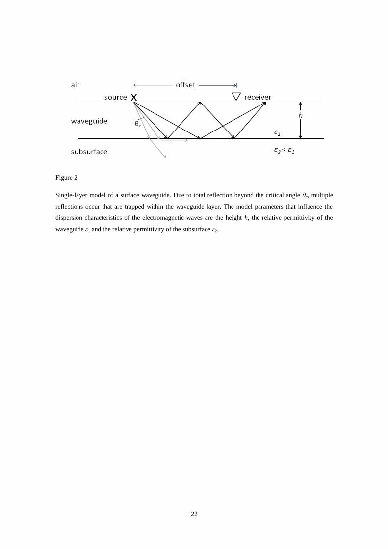
We argue that the posterior parameter distributions presented in Figure 11 (bottom row) best

summarize the actual subsurface properties considered herein based on the results of our

synthetic study. It is demonstrated that the model parameters can only be correctly retrieved

when the full frequency bandwidth together with a heteroscedastic measurement error is used or

a meaningful a-priori reduction to the frequency bandwidth is applied. The latter approach is

rather subjective and in practice it remains difficult to pinpoint an appropriate frequency

bandwidth to invert the dispersion curve. Moreover, the synthetic and the experimental case

studies illustrate the strong sensitivity of the model parameters to high and low frequencies and

with a reduction of the frequency bandwidth we risk to lose valuable information. However, the

MCMC inversion approach introduced herein removes the need for subjective selection of the

frequency bandwidth and is especially designed to retrieve the (heteroscedastic) measurement

error and subsurface properties, and their underlying posterior distribution.

Summary and Conclusions

We applied a deterministic and a Bayesian inversion method to synthetic and experimental

on-ground GPR data with waveguide dispersion assuming a single layer model of the subsurface.

Bayesian inversion used DREAM(ZS), a recently developed MCMC method that provides fast

convergence. Unlike deterministic inversion methods, MCMC sampling with DREAM(ZS)

additionally approximates the joint posterior probability distribution of the model parameters,

13

which enables the investigation of parameter uncertainty and sensitivity. Overall, the estimated

‘best’ parameters derived from synthetic and measured dispersion curves depended strongly on

the frequency bandwidth used in the inversion. More precisely, the relative permittivity of the

subsurface below the waveguide was sensitive to the low frequencies of the dispersion curve,

whereas the relative permittivity and the height of the waveguide were sensitive to high

frequencies. Detailed analysis of the synthetic data showed that the measurement error associated

with the dispersion curve was frequency dependent. In particular, the extreme ends of the

dispersion curve were more uncertain. When such frequency-dependent measurement errors were

not properly handled during the inversion, the resulting model parameters were biased. One

possible way to resolve this issue is to remove the low and high frequency parts of the dispersion

curve during the inversion. Although this procedure led to plausible results for both the

deterministic inversion and MCMC simulation with DREAM(ZS), the choice of an appropriate

frequency bandwidth is quite arbitrary. A better solution is presented herein and consists of

estimating the measurement error properties simultaneously with the model parameters. This

resulted in plausible estimates of all three model parameters that compared well with inversion

results for a reduced frequency bandwidth. Moreover, the heteroscedastic measurement error

function derived in our study compared well with a homoscedastic error model and prior

information. Altogether, the Bayesian inversion framework presented herein is entirely objective,

explicitly handles measurement error and parameter uncertainty, and circumvents the need to

make subjective decisions on the frequency bandwidth to be used in the inversion.

Acknowledgements

The DREAM(ZS) algorithm used in this study was provided by the third author (jasper@uci.edu)

and is available upon request.

14

References Arcone S.A. 1984. Field Observations of Electromagnetic Pulse-Propagation in Dielectric Slabs.

Geophysics 49, 1763-1773.

Arcone S.A., Peapples P.R. and Liu L.B. 2003. Propagation of a ground-penetrating radar (GPR) pulse in

a thin-surface waveguide. Geophysics 68, 1922-1933.

Bohidar R.N. and Hermance J.F. 2002. The GPR refraction method. Geophysics 67, 1474–1485.

Bradford J.H. 2008. Measuring water content heterogeneity using multifold GPR with reflection

tomography. Vadose Zone Journal 7, 184-193

Budden K.G. 1961. The Wave-Guide Mode Theory of Wave Propagation. Prentice-Hall Inc., London

Dannowski G. and Yaramanci U. 1999. Estimation of water content and porosity using combined radar

and geoelectrical measurements. European Journal of Environmental and Engineering Geophysics 4,

71–85.

Endres A.L., Clement W.P. and Rudolph D.L. 2000. Ground penetrating radar imaging of an aquifer

during a pumping test. Ground Water 38, 566–576.

Galagedara L.W., Parkin G.W. and Redman J.D. 2003. An analysis of the ground-penetrating radar direct

ground wave method for soil water content measurement. Hydrological Processes 17, 3615-3628.

Garambois S., Senechal P. and Perroud H. 2002. On the use of combined geophysical methods to assess

water content and water conductivity of near-surface formations. Journal of Hydrology 259, 32–48.

Gelman A. and Rubin D.B. 1992. Inference from Iterative Simulation Using Multiple Sequences.

Statistical Science 7, 457-472.

Gerhards H., Wollschlager U., Yu Q., Schiwek P., Pan X. and Roth K. 2008. Continuous and

simultaneous measurement of reflector depth and average soil-water content with multichannel

ground-penetrating radar, Geophysics 73, J15-J23.

Greaves R.J., Lesmes D.P., Lee J.M. and Toksoz M.N. 1996. Velocity variations and water content

estimated from multi-offset, ground-penetrating radar. Geophysics 61, 683–695.

Grote K., Hubbard S. and Rubin Y. 2003. Field-scale estimation of volumetric water content using

ground-penetrating radar ground wave techniques, Water Resources Research, 39, 1321.

Haarder E.B., Looms M.C., Jensen K.H. and Nielsen L. 2011. Visualizing Unsaturated Flow Phenomena

Using High-Resolution Reflection Ground Penetrating Radar. Vadose Zone Journal 10, 84-97.

Hinnell A.C., Ferre T.P.A., Vrugt J.A., Huisman J.A., Moysey S., Rings J. and Kowalsky M.B. 2010.

Improved extraction of hydrologic information from geophysical data through coupled

hydrogeophysical inversion. Water Resources Research 46, W00D40.

Huisman J.A., Hubbard S.S., Redman J.D. and Annan A.P. 2003a. Measuring Soil Water Content with

Ground Penetrating Radar: A Review. Vadose Zone Journal 2, 476-491.

Huisman J.A., Snepvangers J.J.J.C., Bouten W. and Heuvelink G.B.M. 2003b. Monitoring temporal

development of spatial soil water content variation: comparison of ground-penetrating radar and

time domain reflectometry. Vadose Zone Journal 2, 519-529.

Huisman J.A., Rings J., Vrugt J.A., Sorg J. and Vereecken H. 2010. Hydraulic properties of a model dike

from coupled Bayesian and multi-criteria hydrogeophysical inversion. Journal of Hydrology 380,

62-73.

Huisman J.A., Sperl C., Bouten W. and Verstraten J.M. 2001. Soil water content measurements at

different scales: accuracy of time domain reflectometry and ground-penetrating radar. Journal of

Hydrology 245, 48-58.

Irving J. and Singha K. 2010. Stochastic inversion of tracer test and electrical geophysical data to estimate

hydraulic conductivities, Water Resources Research, 46, W11514.

Jacob R.W. and Hermance J.F. 2004. Assessing the precision of GPR velocity and vertical two-way travel

time estimates. Journal of Environmental and Engineering Geophysics 9, 143-153

Lagarias J.C., Reeds J.A., Wright M.H. and Wright P.E. 1998. Convergence properties of the Nelder-

Mead simplex method in low dimensions. Siam Journal on Optimization 9, 112-147.

Lunt I.A., Hubbard S.S. and Rubin Y. 2005. Soil moisture content estimation using ground-penetrating

radar reflection data, Journal of Hydrology, 307, 254-269.

Mosegaard K. and Tarantola A. 1995, Monte Carlo sampling of solutions to inverse problems, J.

Geophys. Res., 100, 12431–12448.

15

Moysey S. and Knight R. 2004. Modeling the field-scale relationship between dielectric constant and

water content in heterogeneous systems. Water Resources Research 40, 10.

Park C.B., Miller R.D., and Xia J.X. 1998. Imaging dispersion curves of surface waves on multi-channel

record. In: Imaging dispersion curves of surface waves on multi-channel record, pp. 1377–1380.

Pettinelli E., Vannaroni G., Di Pasquo B., Mattei E., Di Matteo A., De Santis A. and Annan P.A. 2007.

Correlation between near-surface electromagnetic soil parameters and early-time GPR signals: An

experimental study. Geophysics 72, A25-A28.

Rhim H.C. 2011. Measurements of dielectric constants of soil to develop a landslide prediction system.

Smart Structures and Systems 7, 319-328.

Sambridge M., and Mosegaard K. 2002. Monte Carlo methods in geophysical inverse problems, Reviews

of Geophysics 40, 1009.

Schoups G. and Vrugt J.A. 2010. A formal likelihood function for parameter and predictive inference of

hydrologic models with correlated, heteroscedastic, and non-Gaussian errors. Water Resources

Research 46, 17.

Slob E. 2010. Uncertainty in ground penetrating radar models. Proceedings of 13th International

Conference on Ground Penetrating Radar (GPR) 2010, doi: 10.1109/ICGPR.2010.5550154

Steelman C.M. and Endres A.L. 2010. An examination of direct ground wave soil moisture monitoring

over an annual cycle of soil conditions. Water Resources Research 46, 16.

Steelman C. M., Endres A.L. and van der Kruk J. 2010. Field Observations of Shallow Freeze and Thaw

processes using High-Frequency Ground-Penetrating Radar, Hydrological Processes, Vol. 24, pp.

2022-2033.

Steelman C.M. and Endres A.L. 2011. Comparison of Petrophysical Relationships for Soil Moisture

Estimation using GPR Ground Waves. Vadose Zone Journal 10, 270-285.

Strobbia C. and Cassiani G. 2007. Multilayer ground-penetrating radar guided waves in shallow soil

layers for estimating soil water content. Geophysics 72, J17-J29.

Turesson A. 2006, Water content and porosity estimated from ground-penetrating radar and resistivity,

Journal or Applied Geophysics 58, 99-111,

van der Kruk J. 2006. Properties of surface waveguides derived from inversion of fundamental and higher

mode dispersive GPR data. IEEE Transactions on Geoscience and Remote Sensing 44, 2908-2915.

van der Kruk J., Arcone S.A. and Liu L. 2007. Fundamental and higher mode inversion of dispersed GPR

waves propagating in an ice layer. IEEE Transactions on Geoscience and Remote Sensing 45, 2483-

2491.

van der Kruk J., Steelman C. M., Endres A. L. and Vereecken H. 2009. Dispersion inversion of

electromagnetic pulse propagation within freezing and thawing soil waveguides: Geophysical

Research Letters, 36, L18503–L18507.

van der Kruk J., Jacob R.W. and Vereecken H. 2010. Properties of precipitation-induced multilayer

surface waveguides derived from inversion of dispersive TE and TM GPR data. Geophysics 75,

WA263-WA273.

van der Kruk J., Streich R. and Green A.G. 2006. Properties of surface waveguides derived from separate

and joint inversion of dispersive TE and TM GPR data. Geophysics 71, K19-K29.

van Overmeeren R.A., Sariowan S.V. and Gehrels J.C. 1997. Ground penetrating radar for determining

volumetric soil water content; Results of comparative measurements at two test sites. Journal of

Hydrology 197, 316-338.

Vrugt J.A. and Bouten W. 2002. Validity of first-order approximations to describe parameter uncertainty

in soil hydrologic models. Soil Science Society of America Journal 66, 1740-1751.

Vrugt J.A., ter Braak C.J.F., Gupta H.V. and Robinson B.A. 2009. Equifinality of formal (DREAM) and

informal (GLUE) Bayesian approaches in hydrologic modeling?. Stochastic Environmental

Research and Risk Assessment 23, 1011-1026.

Vrugt J.A., Ter Braak C.J.F., Diks C.G.H., Robinson B.A., Hyman J.M. and Higdon D. 2009.

Accelerating Markov Chain Monte Carlo Simulation by Differential Evolution with Self-Adaptive

Randomized Subspace Sampling. International Journal of Nonlinear Sciences and Numerical

Simulations 10, 273-290.

Vrugt J.A., Ter Braak, C.J.F, Clark, M.P., Hyman, J.M., and Robinson, B. 2008. Treatment of input

uncetainty in hydrologic modeling: Doing hydrology backwards with Markov chain Monte Carlo

simulation. Water Resources Research 44, W00B09.

Westermann S., Wollschläger U. and Boike J. 2010. Monitoring of active layer dynamics at a permafrost

site on Svalbard using multi-channel ground-penetrating radar. Cryosphere 4, 475-487.

16

Wollschläger U., Gerhards H., Yu Q. and Roth K. 2010. Multi-channel ground-penetrating radar to

explore spatial variations in thaw depth and moisture content in the active layer of a permafrost site.

Cryosphere 4, 269-283.

17

Table 1

True parameter values and their prior ranges used for the synthetic and experimental data.

Parameter true parameter min max

ε1 20 10 30

ε2 10 3 20

h 0.25 0.05 1

18

List of captions

Figure 1

Schematic outline of the algorithm. The measured CMP data is transformed into a dispersion curve which

is a combination of the true dispersion curve and measurement error which comprises a wide range of

possible errors. The forward model gives the theoretical dispersion curve. A deterministic and Bayesian

inversion method are applied of which MCMC simulation with DREAM(ZS) can treat measurement error

explicitly.

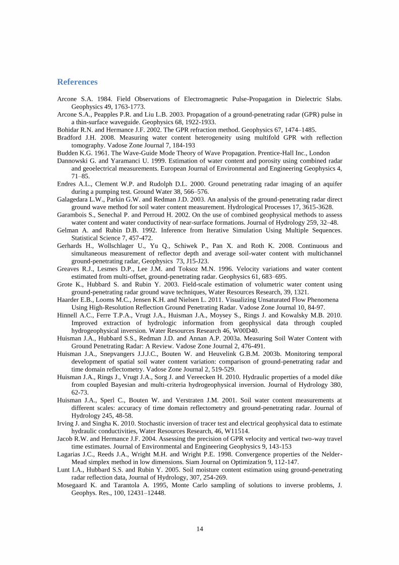
Figure 2

Single-layer model of a surface waveguide. Due to total reflection beyond the critical angle θc, multiple

reflections occur that are trapped within the waveguide layer. The model parameters that influence the

dispersion characteristics of the electromagnetic waves are the height h, the relative permittivity of the

waveguide ε1 and the relative permittivity of the subsurface ε2.

Figure 3

Numerically created CMP data (a) without and (b) with noise, and (c, d) the corresponding phase-velocity

spectra. The theoretical dispersion curve is plotted in green, whereas the picked dispersion curves are

plotted in yellow. The theoretical upper and lower bound of the dispersion curve are indicated with

dashed-dotted white lines. The different frequency ranges used in the inversion are indicated with the

white arrows.

Figure 4

Theoretical dispersion curves with differences in parameter values. In each plot one parameter is varied to

investigate its influence on the dispersion curve. The fixed parameter values are ε1 = 20, ε2 = 10, and height

= 0.25m.

Figure 5

Histograms of the marginal posterior distributions of the model parameters using the dispersion curve

shown in Figure 3c with frequency ranges; a) 43<f<219MHz, b) 71<f<219 MHz, and c) 43<f<145MHz

19

(see also arrows in Figure 3c). These histograms are created using the last 5,000 samples generated with

DREAM(ZS). The green circles represent the results of the deterministic waveguide inversion, the red

triangles denote the mean of the marginal posterior distributions, and the red lines indicate the true

parameter values used to generate the synthetic data.

Figure 6

(a) Average frequency spectra of the noise-free data (Figure 3a), the noisy synthetic data (Figure 3b), and

the noise. (b) Black lines show different realizations of noisy CMP data. The red lines indicate the

standard deviation from the mean of all dispersion curves (68% of all the dispersion curves lay between

the red lines). (c) Three different measurement error variances: σ1me

(blue line) is the homoscedastic

measurement error, which is determined from the RMSE of the best fit to the data, σ2me

(green line) is

obtained by limiting the frequency range of the dispersion curve to 45<f<201 MHz, σ3me

(f) (red line) is

determined from the standard deviation of the 50 different dispersion curve shown in Figure 6b.

Figure 7

Histograms of the marginal posterior parameter distributions corresponding to the dispersion curve shown

in Figure 3d using the three different measurement error variances shown in Figure 6c: a) σ1me

and

34<f<219 MHz, b) σ2me

and 45<f<201, and c) σ3me

(f), and 34<f<219 MHz. The red triangles signify the

mean of the DREAM(ZS) derived marginal posterior distributions, the green dots represent the results of

the deterministic waveguide inversion, and the red lines indicate the true model parameters.

Figure 8

a) Trace-normalized measured CMP data, b) corresponding phase-velocity spectrum using the data

enclosed by the black lines. The yellow line indicates the selected dispersion curve and the different

frequency ranges used in the inversions are indicated with magenta arrows.

Figure 9

Histograms of the marginal posterior parameter distributions using the dispersion curve of Figure 8b and

three different frequency ranges: a) 44-141 MHz, b) 54-141 MHz (low frequency filtered), and c) 44-131

MHz (high frequency filtered). The measurement error is assumed to be frequency independent, normally

distributed with standard deviation similar to the RMSE of the best possible fit to the GPR data. The red

20

triangles denote the mean of the marginal posterior distributions and the green dots illustrate the results of

the determinsitic waveguide inversion.

Figure 10

The estimated homoscedastic and heteroscedastic measurement errors in blue and red, respectively with

their 95 percentile confidence interval. The red dots represent the median of the estimated points and were

used to calculate the median of the heteroscedastic measurement error. The black and green arrows

indicate the RMSE of the best fit of the results shown in Figure 9a and 9c, respectively.

Figure 11

Parameter posterior distributions when measurement error variance σme

and parameter are estimated

simultaneously. In the first row σme

is homoscedastic and in the second row heteroscedastic. The red

triangles denote the mean of the marginal posterior distributions

21

Figure 1

Schematic outline of the algorithm. The measured CMP data is transformed into a dispersion curve which

is a combination of the true dispersion curve and measurement error which comprises a wide range of

possible errors. The forward model gives the theoretical dispersion curve. A deterministic and Bayesian

inversion method are applied of which MCMC simulation with DREAM(ZS) can treat measurement error

explicitly.

22

Figure 2

Single-layer model of a surface waveguide. Due to total reflection beyond the critical angle θc, multiple

reflections occur that are trapped within the waveguide layer. The model parameters that influence the

dispersion characteristics of the electromagnetic waves are the height h, the relative permittivity of the

waveguide ε1 and the relative permittivity of the subsurface ε2.

23

tim

e [

ns]

5 10 15

50

100

150

200

250

phase-v

elo

city [

m/n

s]

50 100 150 200

0.07

0.08

0.09

0.1

theoretical

picked

tim

e [

ns]

offset [m]

5 10 15

50

100

150

200

250

phase-v

elo

city [

m/n

s]

frequency [MHz]

50 100 150 200

0.07

0.08

0.09

0.1

theoretical

picked

(a)

(b)

(c)

(d)

2 = 10

1 = 20 h = 0.25m

c0

1

c0/

2

Figure 3

Numerically created CMP data (a) without and (b) with noise, and (c, d) the corresponding phase-velocity

spectra. The theoretical dispersion curve is plotted in green, whereas the picked dispersion curves are

plotted in yellow. The theoretical upper and lower bound of the dispersion curve are indicated with

dashed-dotted white lines. The different frequency ranges used in the inversion are indicated with the

white arrows.

24

0 200 4000.065

0.07

0.075

0.08

0.085

0.09

0.095

0.1p

ha

se

-ve

locity [m

/ns]

frequency [MHz]

1 =18

1 =19

1 =20

1 =21

1 =22

0 200 400

0.07

0.08

0.09

0.1

0.11

frequency [MHz]

2 =8

2 =9

2 =10

2 =11

2 =12

0 200 4000.065

0.07

0.075

0.08

0.085

0.09

0.095

0.1

frequency [MHz]

h =0.15

h =0.2

h =0.25

h =0.3

h =0.35

Figure 4

Theoretical dispersion curves with differences in parameter values. In each plot one parameter is varied to

investigate its influence on the dispersion curve. The fixed parameter values are ε1 = 20, ε2 = 10, and height

= 0.25m.

25

19.6 20 20.40

0.2

0.4

9.9 10 10.10

0.2

0.4

a) 43 f 219 MHz

0.24 0.25 0.260

0.2

0.4

19.6 20 20.40

0.2

0.4

ma

rgin

al p

rob

ab

ility

9.9 10 10.10

0.2

0.4

b) 71 f 219 MHz

0.24 0.25 0.260

0.2

0.4

19.6 20 20.40

0.2

0.4

1

9.9 10 10.10

0.2

0.4

2

c) 43 f 145 MHz

0.24 0.25 0.260

0.2

0.4

h [m]

Figure 5

Histograms of the marginal posterior distributions of the model parameters using the dispersion curve

shown in Figure 3c with frequency ranges; a) 43<f<219MHz, b) 71<f<219 MHz, and c) 43<f<145MHz

(see also arrows in Figure 3c). These histograms are created using the last 5,000 samples generated with

DREAM(ZS). The green circles represent the results of the deterministic waveguide inversion, the red

triangles denote the mean of the marginal posterior distributions, and the red lines indicate the true

parameter values used to generate the synthetic data.

26

40 60 80 100 120 140 160 180 200 2200

0.5

1

frequency [MHz]

norm

aliz

ed a

mplit

ude

a) average frequency spectrum

noise-free data

noisy data

noise

40 60 80 100 120 140 160 180 200 2200.06

0.08

0.1

frequency [MHz]

phase v

elo

city [

m/n

s]

b) dispersion curves of noisy CMP data

50 noisy dispersion curves

standard deviation

40 60 80 100 120 140 160 180 200 2200

1

2

3

4

x 10-3

frequency [MHz]

phase v

elo

city [

m/n

s]

c) measurement error variance

1me

2me

3me(f)

clipped f or

display

Figure 6

(a) Average frequency spectra of the noise-free data (Figure 3a), the noisy synthetic data (Figure 3b), and

the noise. (b) Black lines show different realizations of noisy CMP data. The red lines indicate the

standard deviation from the mean of all dispersion curves (68% of all the dispersion curves lay between

the red lines). (c) Three different measurement error variances: σ1me

(blue line) is the homoscedastic

measurement error, which is determined from the RMSE of the best fit to the data, σ2me

(green line) is

obtained by limiting the frequency range of the dispersion curve to 45<f<201 MHz, σ3me

(f) (red line) is

determined from the standard deviation of the 50 different dispersion curve shown in Figure 6b.

27

20 22 240

0.2

0.4

10 10.2 10.4 10.60

0.2

0.4

a) 1me and 34 < f < 219MHz

0.15 0.2 0.250

0.2

0.4

20 22 240

0.2

0.4

10 10.2 10.4 10.60

0.2

0.4

b) 2me and 45 < f < 201MHz

0.15 0.2 0.250

0.2

0.4

20 22 240

0.2

0.4

1

10 10.2 10.4 10.60

0.2

0.4

2

c) 3me(f) and 34 < f < 219MHz

0.15 0.2 0.250

0.2

0.4

h[m]

marg

inal pro

babili

ty

Figure 7

Histograms of the marginal posterior parameter distributions corresponding to the dispersion curve shown

in Figure 3d using the three different measurement error variances shown in Figure 6c: a) σ1me

and

34<f<219 MHz, b) σ2me

and 45<f<201, and c) σ3me

(f), and 34<f<219 MHz. The red triangles signify the

mean of the DREAM(ZS) derived marginal posterior distributions, the green dots represent the results of

the deterministic waveguide inversion, and the red lines indicate the true model parameters.

28

time [ns]

offset [m]

10 20 30

100

200

300

400

500

600

phase v

elo

city

[m

/ns]

frequency [MHz]

40 60 80 100 120 1400.08

0.085

0.09

0.095

0.1

0.105

0.11

0.115a) b)

Figure 8

a) Trace-normalized measured CMP data, b) corresponding phase-velocity spectrum using the data

enclosed by the black lines. The yellow line indicates the selected dispersion curve and the different

frequency ranges used in the inversions are indicated with magenta arrows.

29

20 21 220

0.2

0.4

0.6

7.45 7.5 7.550

0.2

0.4

0.6a) 44 f 141 MHz

0.17 0.18 0.190

0.2

0.4

0.6

20 21 220

0.2

0.4

7.45 7.5 7.550

0.2

0.4

b) 54 f 141 MHz

0.17 0.18 0.190

0.2

0.4

20 21 220

0.2

0.4

1

7.45 7.5 7.550

0.2

0.4

2

c) 44 f 131 MHz

0.17 0.18 0.190

0.2

0.4

h[m]

ma

rgin

al p

rob

ab

ility

Figure 9

Histograms of the marginal posterior parameter distributions using the dispersion curve of Figure 8b and

three different frequency ranges: a) 44-141 MHz, b) 54-141 MHz (low frequency filtered), and c) 44-131

MHz (high frequency filtered). The measurement error is assumed to be frequency independent, normally

distributed with standard deviation similar to the RMSE of the best possible fit to the GPR data. The red

triangles denote the mean of the marginal posterior distributions and the green dots illustrate the results of

the determinsitic waveguide inversion.

30

Figure 10

The estimated homoscedastic and heteroscedastic measurement errors in blue and red, respectively with

their 95 percentile confidence interval. The red dots represent the median of the estimated points and were

used to calculate the median of the heteroscedastic measurement error. The black and green arrows

indicate the RMSE of the best fit of the results shown in Figure 9a and 9c, respectively.

31

20 21 220

0.2

0.4

0.6

7.45 7.5 7.550

0.2

0.4

0.6a) with estimated

me (homoscedastic)

0.17 0.180.190

0.2

0.4

0.6

20 21 220

0.2

0.4

1

7.45 7.5 7.550

0.2

0.4

2

b) with estimated me

(f) (heteroscedasctic)

0.17 0.180.190

0.2

0.4

h

ma

rgin

al p

rob

ab

ility

Figure 11

Parameter posterior distributions when measurement error variance σme

and parameter are estimated

simultaneously. In the first row σme

is homoscedastic and in the second row heteroscedastic. The red

triangles denote the mean of the marginal posterior distributions