1

INVERSE DEMAND RELATIONSHIPS FOR WHEAT FOOD USE BY CLASS

Thomas L. Marsh Associate Professor

Department of Agricultural Economics Kansas State University Manhattan, KS, 66506 phone: 785-532-4913

fax: 785-532-6925 email: tlmarsh@agecon.ksu.edu

Allen M. Featherstone Professor

Department of Agricultural Economics Kansas State University Manhattan, KS, 66506

email: afeather@agecon.ksu.edu

Paper prepared for presentation at the American Agricultural Economics Association Annual Meeting, Montreal, Canada, July 27-30, 2003

Copyright 2003 by Thomas L. Marsh and Allen M. Featherstone. All rights reserved. Readers may make verbatim copies of this document for non-commercial purposes by any means, provided that this copyright notice appears on all such copies.

2

Abstract: A normalized quadratic input distance system is applied to estimate inverse demand relationships for wheat by class. Semi-nonparametric and Bayesian estimators are used to impose curvature on inputs and outputs. Price flexibilities are estimated for hard red winter, hard red spring, soft red wheat, soft white winter, and durum wheat. Durum wheat is found to be the most price flexible. Economically and statistically important differences in price formation across classes of wheat are found and are supportive of government programs differentiating wheat by class.

3

Introduction Policymakers in the U.S. have been recently altered and introduced farm programs that recognize

differences in demand and supply responses for wheat classes. For example, the Commodity Credit

Corporation (CCC) released market loan rates by class “to establish loan rates that are in line with

market forces in order to avoid over-production of wheat in a county in response to the benefits that are

available under the marketing loan program” (U.S. Department of Agr iculture 2002). To better

understand price formation and market response for wheat food use, we conceptualize and specify an

industry distance function with the different wheat classes as an input into flour production. A

normalized quadratic distance function is used from which a factor demand system and flexibilities are

derived and then jointly estimated with the distance function itself. Moreover, an interesting empirical

digression on comparing alternative approaches to imposing curvature is provided.

Previous research on wheat by class is limited. Chai (1972) estimated domestic demand for

wheat by class over the period from 1929 to 1963. Chai concluded that price elasticities were more

elastic for hard classes than soft classes of wheat. Barnes and Shields (1998) estimated a double- log

demand system for wheat by class. Annual data from 1981 to 1998 were used in a demand system

analysis with regional prices at the farm level. Inelastic own-price elasticities were reported for each of

the five wheat classes, but different from Chai, soft white wheat was reported as being the most elastic

and durum being the least elastic. Wilson and Gallagher (1990) examined price responsiveness for

wheat classes using a Case function approach and found important quality differentials in international

markets. Marsh (2003) reported cost, price, and substitution elasticities for hard red winter, hard red

spring, soft red wheat, soft white winter, and durum wheat over the period 1974-1999. In general, hard

red winter and spring wheat varieties were much more responsive to their own price than were soft

wheat varieties and durum wheat.

4

Previous research on normalized quadratic distance functions is also limited. On the consumer

demand side, Holt and Bishop (2002) recently specified a normalized quadratic distance function and

used it to estimate inverse demand relationships for fish. In contrast, our focus is on the production side

where we apply an alternative functional form of the normalized quadratic function for an input distance

function (Marsh, Featherstone, and Garrett 2003). The normalized quadratic input distance function

specified in the current study accommodates both single and multiple output production processes and

allows direct testing or imposition of input and output curvature conditions. Even for the case of a

single input where the properties of the consumer and input distance function are equivalent (Cornes

1992), the functional specification is different.

Several approaches are compared that estimate the distance function jointly with the inverse

demand functions and impose curvature restrictions. To do this we exploit the stochastic frontier

approach (Stevenson 1980; Greene 1980; Battese and Coelli 1988), which effectively estimates the

objective function itself, and extend the approach to include inverse demand relationships. This

framework is sufficiently flexible to impose curvature on both inputs and outputs, as well as allow

estimation of a complete system of equations. For this input distance system, we first explore a semi-

nonparametric estimator with curvature conditions imposed following Lau (1978). Next, we explore a

parametric estimator that uses a maximum likelihood function for a complete system of equations to

construct a Bayesian model with curvature restrictions imposed following Geweke (1986). This

research compliments recent studies by Atkinson and Primont (2002) and Atkinson, Färe, and Primont

(2003), who estimated complete systems of inverse demand relationships jointly with the distance

function using a GMM estimator. However, neither study specified a likelihood function for the

complete system of equations nor did they consider curvature restrictions.

5

The paper proceeds in the following manner. First, a normalized quadratic input distance

function is specified. Second, the data for the empirical analysis are discussed. Third, the empirical

model and key econometric issues are presented, including curvature restrictions and the maximum

likelihood function for a complete system of equations with extensions to a Bayesian estimator. Fourth,

results are reported and interpreted. This includes empirical inverse demand relationships for wheat by

class and price flexibilities. Finally, implications and concluding comments are provided.

Normalized Quadratic Input Distance Function

Input-Distance Function

The direct input distance function is defined by

(1)

where 1δ ≥ . In (1), y is a (m× 1) vector of outputs, x =(x1,…,xk)′ is a (n × 1) vector of inputs and ( )S y

is the set of all input vectors n+∈x R that can produce the output vector m

+∈y R . The underlying

behavioral assumption is that the distance function represents a rescaling of all the input levels

consistent with a target output level. Intuitively, δ is the maximum value by which one could divide x

and still produce y. The value δ places / δx on the boundary of ( )S y and on the ray through x.

Investigating the distance function is interesting because it is a dual representation of the cost function

and both are valid representations of multiple output technologies. The input distance function measures

the extent to which the firm is input inefficient in producing a fixed set of output. Moreover, it provides

direct estimates of input inefficiency and price flexibilities that are informative economic measures of

price formation.

The standard properties of a distance function are that it is homogenous of degree one,

nondecreasing, and concave in input quantities x, as well as nonincreasing and quasi-concave in outputs

( ) { }, sup 0 | ( / ) ( ), MD S y +δ

= δ > δ ∈ ∀ ∈x y x y R

6

y (Shephard 1970; Färe and Primont 1995). From this framework, inverse factor demand equations may

be obtained by applying Gorman’s Lemma

(3)

where p*=(p1,…,pn)′ is a (n × 1) vector of cost normalized input prices or *1

/n

i i j jjp p p x

== ∑ . The

Hessian matrix is given by the second order derivatives of the distance function (Antonelli matrix)

(4)

2 2

2 2

( , ) ( , )

( , ) ( , )

D D

AD D

∂ ∂ ′ ′∂ ∂ ∂ ∂ = ∂ ∂

′ ′∂ ∂ ∂ ∂

x y x yx x x y

x y x yy x y y

The input distance function is often used as a measure of technical efficiency (Farrell 1957;

Debreu 1951). Inefficiencies arise if firms do not use cost minimizing amounts of input for several

reasons, including regulated production, production quotas, or shortages (Atkinson and Primont 2002;

Atkinson, Färe, and Primont 2003). The input-oriented measures of technical efficiency is given by

(5) { }1/ inf : ( )TE D x Sδ

= = δ δ ∈ y

where TE lies between zero and one. This efficiency measure can be equivalently specified as

(6) ln ln ln 0D TE D u+ = − =

where the term lnu TE= − can be expressed as exp( )TE u= − . Hence, u is nonnegative being bounded

below by zero and unbounded from above.

Normalized Quadratic Distance Function

To complete the model specification, the inverse demand equations in (3) are derived from a

normalized quadratic distance function (Marsh, Featherstone, and Garrett 2003). The normalized

*( , )( , )

D∂=

∂x y

p x yx

7

quadratic allows estimation of flexibilities, as well as the explicit investigation of the interactions

between inputs and outputs. The proposed normalized quadratic distance function is given by

(7) 1

01 1 1 1 1 1 1 1 1

1( , )

2

n n m n n n n m n m n n m

i i i i k k ij i j ij i j ij i ji i n k i j i n j n i j n

D y b b x b y x b x x b y y b x y−+ + + +

= = + = = = = + = + = = +

= + + + α + +

∑ ∑ ∑ ∑∑ ∑ ∑ ∑ ∑x

with n inputs and m outputs. The ' and 'i ijb s b s are parameters to be estimated, while the iα are

predetermined positive constants that dictate the form of normalization. Symmetry is imposed by

restricting ij jib b= . The normalized quadratic distance function in (7) is semiflexible at a reference

vector *x (Diewert and Wales 1988).

Using Gorman’s Lemma, the input demand equations are given by

(8) 1 2

*

1 1 1 1 1 1

n n n n n n m

i i k k ij j i k k ij i j ij jk j k i j j n

p b x b x x b x x b y− − +

= = = = = = +

= + α + α α +

∑ ∑ ∑ ∑∑ ∑

where the input prices are normalized as *1

/n

i i j jjp p p x

== ∑ such that cost of producing the target level

of output is unity. Homogeneity of degree ze ro in inputs in the input demand equations implies that

1

0n

ijj

b=

=∑ , while the normalization restriction requires that 1

1n

k kk

x=

α =∑ at a reference vector. The

equivalent share equation is given by

(9) 1 2

1 1 1 1 1 1

n n n n n n m

i i i k k ij j i i i k k ij i j ij j ik j k i j j n

w b x x b x x x x b x x b y x− − +

= = = = = = +

= + α + α α +

∑ ∑ ∑ ∑∑ ∑

Normalizing quantities by their mean values yields unit means, or * (1,...,1) nx l′= = , which can be used

as a reference bundle. At a reference vector *x , the demand restrictions become

(10) *

1 1

1n n

k k kk k

x= =

α = α =∑ ∑ , 0,k kα ≥ ∀ , and *

1 1

0n n

j ij ijj j

x b b= =

= =∑ ∑

8

Given the distance function is homogeneous of degree one quantities, then it is possible to

normalize by some λ (e.g., an input or output or convex combinations),

(11) ( ) ( )* *1, , ln , ln ln ,D D D D = ⇔ − λ = λ λ λ

x xx y y x y y

From (6) the relationship can be rewritten as

(12) *ln ln ,D u − λ = − λ

xy

In empirical applications, the term lnu TE= − has been exploited to form an estimable equation of the

distance function itself that provides a direct measure of input inefficiency (Stevenson 1980; Greene

1980; Battese and Coelli 1988; Morrison Paul, Johnston, and Frengley 2000; Brümmer, Glauben, and

Thussen 2002). Alternatively, Atkinson and Primont (2002) and Atkinson, Färe, and Primont (2003)

directly estimate equations (6) with generalized methods of moments.

Compensated price flexibilities at * (1,...,1) nx l′= = are given by the equation

(13) * lnln

ij jiij

j i

b xpf

x p∂

= =∂

for i, j=1,…,n

using the estimated ijb and the predicted ip .

Stochastic Input-Normalized Distance System

To define a distance function normalized by the kth input let * 1,...,s s kx x x s n= ∀ = . Define the

predetermined constants as (0,...,0, ,0...,0) 1k kα = α ∋ α = , then *

1

1 n

s ss

x=

α =∑ . Using the homogeneity

property of the distance function, it can be written as

(14) 1 1 1 1

* * * * * * * *0

1 1 1 1 1 1 1 1

( / , ) 1( , )

2

n n m n n n m n m n n mk

i i i i ij i j ij i j ij i ji i n i j i n j n i j nk

D x yD y b b x b y b x x b y y b x y

x

− + − − + + − +

= = + = = = + = + = = +

= = + + + + +

∑ ∑ ∑∑ ∑ ∑ ∑ ∑x

x

9

Hence, the distance function in (14) is a special case of that in (7). The input demand functions for (14)

become

(15) 1

* * * * *

1 1

for 1,..., 1n n m

i i ij j ij j ij j n

p b b x b y i n− +

= = +

= + + + ε = −∑ ∑

with stochastic error terms iε . Flexibilities follow those specified in (13).

From (11) the kth input-normalized distance function can be represented by

(16) 1 1 1 1

* * * * * * *0 0

1 1 1 1 1 1 1 1

1ln

2

n n m n n n m n m n n m

k i i i i ij i j ij i j ij i ji i n i j i n j n i j n

x b b x b y b x x b y y b x y u− + − − + + − +

= = + = = = + = + = = +

− = + + + + + − + ε

∑ ∑ ∑∑ ∑ ∑ ∑ ∑

where 0ε is assumed to be an identically distributed stochastic error term and independent of u. This

representation is important because estimation of the demand equations [equation (15)] without the

distance functions in (16) limits curvature testing and imposition to inputs and not outputs.

Alternatively, estimating a system including (15) and (16) offers opportunity to impose the complete set

of curvature restrictions defined in (4) and potentially increase econometric efficiency. We assume cross

correlation of the ' 0,1,..., 1i s i nε = − with covariance *S , but independence among the u and

' 0,1,..., 1i s i nε = − . Estimation issues concerning (16) are complicated by that fact that u is

unobserved, but have been addressed in several ways in the stochastic frontier production literature,

which we discuss in more detail below.

Data

Annual prices and quantities for the empirical analysis for each of the five wheat classes are based on

June to May marketing years, from 1974/1975 to 1999/2000. Descriptive statistics are provided in

Table 1. Wheat quantity and price data were collected from U.S. Department of Agriculture’s Economic

Research Service, Wheat Year Book, annually from 1974 to 2001. Total flour production increased from

251 million cwt in 1974 to 412 million cwt in 1999, averaging 332 million cwt over the period. Total

10

wheat food use (the sum of HRW, HRS, SRW, SWW, and DUR food use) has increased from 545 million

bushels in 1974 to 925 million bushels in 1999. Figure 1 presents food use by wheat class, showing

food use has been trending upwards over time. From 1974 to 1999 the average proportion of total food

use was 0.42, 0.25, 0.19, 0.07, and 0.07 for HRW, HRS, SRW, SWW, and DUR, respectively.

Given the importance of protein content for hard wheat varieties in flour production, we estimate

the empirical model with wheat cash prices from major markets. This is because HRW and HRS prices

are sensitive to protein content across regions (Parcell and Stiegert 1998) and that these quality impacts

from protein may be averaged out in the regional price data (Marsh 2003). In particular, the HRW price

is represented by Kansas City, No.1 (13% protein); HRS price by Minneapolis, dark No.1 spring (13%

protein); SRW price by Chicago, No. 2; SWW price by Portland No.1; and DUR by Minneapolis, No.1

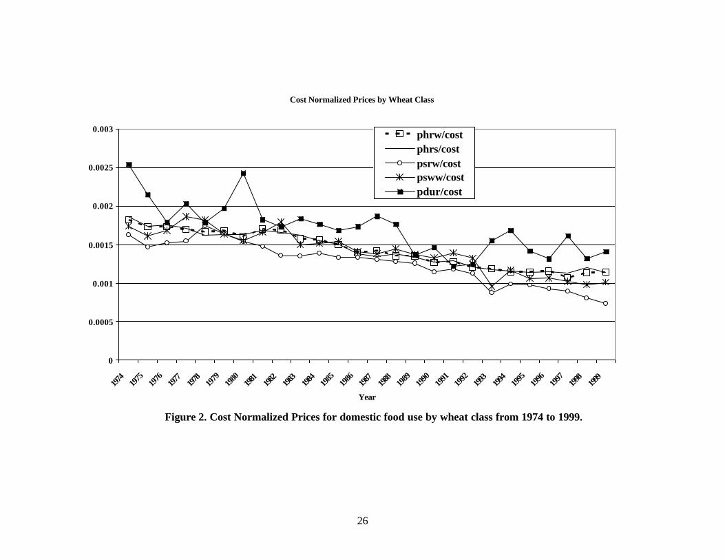
hard amber durum. Figure 2 shows cost normalized prices for wheat by class.

Econometric Estimation

Following Wholgenant (1989) and Marsh (2003), the raw product is considered as an input into food

production. Hence, we specify an industry distance function for the flour milling industry and derive

inverse factor demand equations. In specification of the distance function, we do not differentiate

between types of flour produced, but rather assume flour output is a homogeneous product. Although

this is a simplification, the assumption is empirically practical because of limited quantity data for flour.

Finally, millfeed output is not considered in the conceptual model specification. This is because millfeed

is a by-product of flour milling that is used as feed input in the livestock industry and prices typically

follow other feed stuffs such as corn prices (Harwood et al., 1989).

The econometric system consists of the four inverse factor demand equations in (15) and the

transformed distance function in (16), including HRW, HRS, SRW, and SWW. DUR quantity was used to

11

normalize the distance function. Flexibilities were recovered for the DUR equation using standard

properties of general demand restrictions.

Curvature

In this analysis we consider two approaches to imposing curvature, including Choleskey decomposition

and Bayesian estimation. The Choleskey decomposition approach for the normalized quadratic only

requires reparameterization of the Hessian matrix. For example, to impose concavity the Antonelli

matrix can be reparameterized into a negative semidefinite matrix by ′= −A BB where B is a lower

triangular matrix (Lau 1978). Under the Bayesian framework, demand restrictions are imposed

following Geweke (1986) and imposing uniform priors on parameters of interest. Griffith, O’Donnell,

and Cruz (2000) also use Geweke’s approach to imposing restrictions using the Metropolis-Hastings

algorithm.

Semi-Nonparametric Estimation

Consider the error term 0v u= ε − from (16). Because the term lnu TE= − is an unobservable

independent variable, specification of equation (16) requires further assumptions to achieve econometric

identification and subsequent estimation. However, standard procedures in the stochastic frontier

literature are to assume the unobservable variable u is represented by a distribution with nonegative

support and with mean µ . Most often the choice has been the truncated normal or a gamma distribution

(see Stevenson 1980; Greene 1980; Battese and Coelli 1988). Following Morrison Paul, Johnston, and

Frengley (2000), Brümmer, Glauben, and Thussen (2002), the mean µ can be specified as a function of

observable predetermined variables Z, or ( , )fµ = γZ , with unknown parameters γ . The γ parameters

are then estimated by directly substituting ( , )fµ = γZ into (16). This approach is similar to Zellner’s

(1970) instrumental variable approach to unobservable independent variables that provides consistent

parameter estimates.

12

Initially, we follow a fixed effect approach and specify Z as discrete shift variables representing

technical efficiency over the periods from 1974-1980, 1981-1990, and 1991-1999. The system of

equations represented by (15) and (16) with fixed effects is estimated using a method of moments

estimator. Atkinson and Primont (2002) point out that neither the fixed nor random effect dominate one

another. For a fixed effect specification, identification can be difficult. While for a random effects

specification, strong distributional assumptions are made about the distributions of the error. The

random effect specification is taken up when we apply a maximum likelihood estimator of the system of

equations in (15) and (16).

To measure the significance of price and substitution flexibilities, bootstrapped confidence

intervals are constructed. Bootstrap procedures are convenient for intractable inference problems and

are often equivalent or superior to first-order asymptotic results (Mittelhammer, Judge, and Miller

2000). Bootstrap estimates are obtained by (a) resampling the residuals of the model, (b) predicting cost

and prices of wheat, (c) reestimating the five-equation system with predicted values, and (d) then

recalculating the flexibilities. This process was repeated 500 times to generate distributions of cost,

price, and substitution flexibilities. Then 90% confidence intervals for each flexibility were constructed

based on the percentile method, which requires ordering the estimated flexibilities and then selecting

outcome 25 (0.05*500) for the lower critical value and outcome 475 (0.95*500) for the upper critical

value. For hypothesis testing, if the bootstrapped confidence interval for the flexibility contains zero,

then the flexibility value is not considered significantly different from zero at the 0.10 level.

Parametric Estimation

To derive a likelihood function of (15) and (16) with a random effects component, the error term

0v u= ε − is specified as the sum of a truncated normal with mean µ and variance 2uσ and the

'i sε are distributed ( )*,N 0 S . Further, the u are distributed independently of the 'i sε . Using a

13

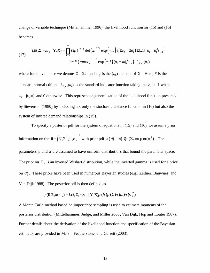
change of variable technique (Mittelhammer 1996), the likelihood function for (15) and (16)

becomes

(17) ( ) ( ){ }( )

( ) { }( )

/ 2

[0, )

1 / 2 211

1

1

( , , , | , ) (2 )

( )

det exp .5 2 [.,1]

1 exp .5 ( )

TT

u t t t t tt

u t u t

L

I u

u u

F u

µ σ π ε ε ε σ

µ σ µ σ

−

∞

=

−

Σ = ′ ′Σ − Σ + Σ +

− − − −

∏ß Y X

where for convenience we denote 1*−Σ = Σ and ijσ is the (i,j) element of Σ . Here, F is the

standard normal cdf and [0, ) ( )iI u∞ is the standard indicator function taking the value 1 when

[0, )iu ∈ ∞ and 0 otherwise. This represents a generalization of the likelihood function presented

by Stevenson (1980) by including not only the stochastic distance function in (16) but also the

system of inverse demand relationships in (15).

To specify a posterior pdf for the system of equations in (15) and (16), we assume prior

information on the ( )*, , , u

′′′θ = β Σ µ σ with prior pdf 2* u( ) ( ) ( ) ( ) ( )π θ = π β π Σ π µ π σ . The

parameters and β µ are assumed to have uniform distributions that bound the parameter space.

The prior on *Σ is an inverted Wishart distribution, while the inverted gamma is used for a prior

on 2uσ . These priors have been used in numerous Bayesian studies (e.g., Zellner, Bauwnes, and

Van Dijk 1988). The posterior pdf is then defined as

2( , , , ) ( , , , | , ) ( ) ( ) ( ) ( )u u up LΣ = Σ Σß ß Y Xµ σ µ σ π β π π µ π σ

A Monte Carlo method based on importance sampling is used to estimate moments of the

posterior distribution (Mittelhammer, Judge, and Miller 2000; Van Dijk, Hop and Louter 1987).

Further details about the derivation of the likelihood function and specification of the Bayesian

estimator are provided in Marsh, Featherstone, and Garrett (2003).

14

Results and Discussion

Semi-Nonparametric Estimation

Parameter estimates, asymptotic standard errors, and 90% bootstrapped confidence intervals are

presented in Table 2 for the model with symmetry and curvature imposed using Cholesky

decomposition. Based on the bootstrapped confidence intervals, sixteen of the twenty-five estimated

coefficients are statistically significant at the 0.10 level. The output coefficients are negative and

significant at the 0.10 level for each demand equation. R-square values, which explain variation in

quantity of wheat for food use, were 0.997, 0.966, 0.969, 0.920, and 0.894 for the distance function,

HRW, HRS, SRW, and SWW, respectively.

Linear (b1t) and quadratic (b1t) time trend and efficiency (b1970 and b1990) parameters were also

significant. The time trend coefficients indicate a quadratic upwards trend over time, representing

potential technical change and other factors. The parameters representing technical efficiency from the

periods 1974-1980 and 1991-1999 yielded nearly identical technical efficiency values of 0.983 and

0.985, respectively. These results complement those reported by Hossain and Bhuyan (2000) who

estimated an output distance function and found that productivity growth in the flour sector (SIC 2041)

from 1960-1994 came primarily from technical change rather than change in efficiency.

Table 3 contains price flexibilities at the mean for each demand equation. Signs of the own-

flexibilities were negative as required with the imposition of concavity and are inflexible for each wheat

class. Durum wheat exhibits the own-flexibility with the largest magnitude (-0.74), while the own-

flexibility of the remaining wheat classes range from -0.03 to -0.22. Cross-price effects are inflexible.

Bayesian Estimation

Bayesian parameter estimates and 90% confidence intervals are presented in Table 4. Seventeen of the

twenty-four coefficients are statistically significant at the 0.10 level. The output coefficients are

15

negative and significant at the 0.10 level for each demand equation. The trend coefficients indicate an

increasing upwards trend, but at a slower rate than that of the semi-nonparametric model. The parameter

µ representing mean technical efficiency yielded an estimate for technical efficiency with a value of

0.896.

Table 5 contains the mean price flexibilities for each demand equation. Signs of the own-

flexibilities were negative as required with the imposition of concavity and are inflexible for each wheat

class. Durum wheat exhibits the own-flexibility with the largest magnitude (-0.94) followed by hard red

winter wheat (-0.52), while the own-flexibility of the remaining wheat classes range from -0.13 to -0.37.

Cross-price effects are also inflexible. Only the cross-effects between HRW and DUR are statistically

significant.

Discussion

Comparing across the estimators, the price flexibilities were all inelastic. However, the own-price

flexibilities were larger (especially for HRW and HRS) from the Bayesian estimation relative to those

from the semi-nonparametric estimation. In contrast, the trend variables were less prominent in the

Bayesian estimator. Interestingly, the measures of input inefficiency were relatively similar.

Overall, durum wheat is the most price flexible over the sample. Revisiting Figure 2, which

presents the cost normalized prices by wheat class, clearly exhibits that durum wheat has the most price

volatility over the sample period. This is not surprising given its limited geographical production and

stringent quality requirements. Moreover, it has limited substitutability with the exception of high

quality hard red wheat (Barnes and Shields 1998). Soft white wheat exhibits the least flexibility. Mean

price flexibilities across the two estimators for soft white wheat range from -0.10 to -0.13. Meanwhile

soft red winter wheat ranges from -0.22 to -0.35. The difference in the mean price flexibilities across

the estimators is surprising for hard red spring and winter wheat. Intuitively, the higher price

16

flexibilities from the Bayesian estimator seem more reasonable because they are higher quality wheat

and prices depend on protein content (Parcell and Stiegert 1998; Bale and Ryan 1977).

Conclusions

We conceptualized and specified a normalized quadratic input distance function from which to derive

inverse demand functions for the different wheat classes as an input into flour production. A semi-

nonparametric estimator with fixed effects for input inefficiency and a Bayesian estimator with random

effects for input inefficiency (both imposing curvature restrictions) were used to estimate a complete

system of equations (distance function and inverse demand relationships) and to calculate price

flexibilities for wheat food use by class.

Empirical findings of this study are important to policymakers. Overall, results were relative ly

robust across estimators in that the own-price flexibilities were all inelastic. Durum wheat exhibited the

own-flexibility with the largest magnitude (-0.74 to -0.94), while the own-flexibilities of soft red winter

(-0.22 to -0.35) and soft white (-0.10 to -0.13) wheat were relatively consistent across the two

estimators. In contrast, hard red winter and hard red spring wheat exhibited larger changes in own-price

flexibilities across the two estimators. Hard red winter wheat ranged from -0.03 to -0.52, while hard red

spring wheat ranged from -0.10 to -0.37. Nevertheless these results indicate important differences in

price formation across wheat classes and are supportive of government programs that no longer assume

wheat to be a homogenous product. Programs that differentiate wheat by class address concerns of

surplus (and other) problems arising from government policies that distort price spreads between

different types and qualities of wheat (e.g., Farnsworth 1961).

17

Table 1. Descriptive statistics for nominal price and quantity data from 1974 to 1999. Variable Mean St. Dev. Min Max Quantity of Flour (1000 cwt) 332090.00 51405.00 251100.00 411970.00 Price of Hard Red Winter ($US/bu) 3.93 0.66 2.81 5.69 Price of Hard Red Spring ($US /bu) 3.94 0.67 2.83 5.64 Price of Soft Red Wheat ($US /bu) 3.43 0.63 2.19 4.83 Price of Soft White Wheat ($US /bu) 3.86 0.61 2.90 5.27 Price of Durum ($US /bu) 4.74 1.11 3.30 7.03 Quantity of Hard Red Winter (million bu) 305.35 45.95 251.00 387.00 Quantity of Hard Red Spring (million bu) 178.46 39.52 128.00 260.00 Quantity of Soft Red Wheat (million bu) 133.65 17.10 94.00 155.00 Quantity of Soft White Wheat (million bu) 54.23 14.50 31.00 85.00 Quantity of Durum (million bu) 53.15 17.63 32.00 80.00

18

Table 2. Semi-Nonparametric parameter estimates from the normalized quadratic system. Study period from 1974 to 1999.a Coefficient

Coefficient Estimate t-value p-value

b0 -4.25930* -3.37861 0.00073 b1 3.07246* 23.41018 0.00000 b2 2.66231* 19.06190 0.00000 b3 3.81680* 13.26632 0.00000 b4 3.87449* 12.19213 0.00000 b5 2.41177* 5.73059 0.00000 b11 0.08385* 2.27983 0.02262 b12 -0.19495* -2.75455 0.00588 b13 0.17115 0.65944 0.50961 b14 0.26480 0.85603 0.39198 b22 0.04855 0.16040 0.87257 b23 0.08073 0.04513 0.96400 b24 0.26063 0.59963 0.54875 b33 0.26194 0.31598 0.75202 b34 -0.00327 -0.00172 0.99862 b44 -0.00003 0.00000 1.00000 b15 -0.47943* -18.37210 0.00000 b25 -0.39437* -14.60137 0.00000 b35 -0.66601* -11.61678 0.00000 b45 -0.64058* -10.59324 0.00000 b55 -0.00006 0.00000 1.00000 b1t -2.64166* -5.07957 0.00000 b2t 0.73554* 2.93002 0.00339 b1970 0.01725* -2.17105 0.02993 b1990 0.01549* -2.58818 0.00965 a Quantity of flour was scaled by 100,000 in estimation. * Significant at 10% level.

19

Table 3. Semi-Nonparametric price flexibility estimates from the normalized quadratic system with bootstrapped 90% percentile confidence intervals.

Equation Price Cholesky Decomposition Price Flexibilities HRW HRS SRW SWW DUR HRW -0.03000* 0.06969 -0.06946 -0.09552 0.17064 HRS 0.04021 -0.09920* 0.08216 0.09665 -0.16227 SRW -0.02719 0.05574 -0.22441* -0.12513 0.53143* SWW -0.01663 0.02915 -0.05563 -0.10422* 0.20169* DUR 0.03361 -0.05538 0.26733* 0.22822* -0.74150* *90% confidence interval does not contain zero.

20

Table 4. Bayesian Regression estimates and confidence intervals from the normalized quadratic system. Study period from 1974 to 1999.a

Coefficient

Coefficient Estimate

90% Confidence

Interval (Lower)

90% Confidence

Interval (Upper)

b0 -4.26837* -4.35244 -4.17123 b1 3.16721* 2.98338 3.16467 b2 2.63845* 2.57417 2.75 b3 3.91642* 3.72912 3.90753 b4 3.84199* 3.78666 3.95921 b5 2.4766* 2.32197 2.50249 b11 -0.08632* -0.10409 -0.03313 b12 -0.01357 -0.05099 0.06599 b13 0.01381 -0.07089 0.06454 b14 -0.0173 -0.08321 0.06447 b22 -0.02378* -0.13679 -0.03541 b23 -0.02073 -0.05745 0.0818 b24 0.02364 -0.05059 0.09746 b33 -0.11639* -0.19665 -0.04967 b34 -0.07959 -0.12494 0.02557 b44 -0.17926* -0.23322 -0.06696 b15 -0.40074* -0.56946 -0.38792 b25 -0.39817* -0.48715 -0.30291 b35 -0.74633* -0.75767 -0.5788 b45 -0.59522* -0.72857 -0.54998 b55 -0.01033* -0.09562 -0.00439 b1t -0.26847* -0.35138 -0.17638 b2t 0.07288 -0.02305 0.10031 µ 0.10956* 0.04192 0.95994

a Quantity of flour was scaled by 100,000 in estimation. * Significant at 10% level.

21

Table 5. Bayesian Regression price flexibility estimates from the normalized quadratic system with 90% percentile confidence intervals.

Equation Price Bayesian Price Flexibilities HRW HRS SRW SWW DUR HRW -0.52289* -0.02616 -0.06202 -0.07445 0.54002* HRS 0.00472 -0.36521* 0.02397 0.03032 0.16272 SRW -0.01793 0.01688 -0.34736* -0.08047 0.18212 SWW -0.01143 0.01454 -0.0368 -0.13307* 0.05211 DUR 0.54753* 0.35994 0.42222 0.25768 -0.93697* *90% confidence interval does not contain zero.

22

References

Atkinson, S. E. and D. Primont (2002). “Stochastic Estimation of Firm Technology, Inefficiency, and Productivity Growth Using Shadow Cost and Distance Functions,” Journal of Econometrics 108:203-225. Atkinson, S. E. R. Färe, and D. Primont (2003). “Stochastic Estimation of Firm Inefficiency Using Distance Functions,” Southern Economic Journal 69:596-611.

Bale, M.D. and Ryan, M. E. 1977, ‘Wheat protein premiums and price differentials’, American Journal of Agricultural Economics, vol. 59, pp. 530-532. Barnes, J. N. and Shields, D. A. 1998, ‘The growth in U.S. wheat food demand’, Wheat Yearbook, USDA, Economic Research Service, March, pp. 21-29. Battese, G. E. and T. J. Coelli. 1988. “Prediction of Firm-Level Technical Efficiencies with a Generalized Frontier Production Function and Panel Data,” Journal of Econometrics 38:387-399. Brümmer, B., T. Glauben, and G. Thussen. “Decomposition of Productivity Growth Using Distance Functions: The Case of Dairy Farms in Three European Countires,” American journal of Agricultural Economics, 84(3) (August 2002):628-644. Chai, J. C. 1972, The U.S. Food Demand for Wheat by Class, Department of Agricultural and Applied Economics, University of Minnesota. Staff Paper P72-14. Chambers, R. G. 1988. Applied Production Analysis: A Dual Approach, Cambridge University Press, New York. Cornes, R. 1992. Duality and Moden Economics, Cambridge University Press, New York. Debreu, G. (1959). Theory of Value. John Wiley & Sons: New York. Diewert, W. E. and T. J. Wales. 1988. “A Normalized Quadratic Semiflexible Functional Form,” Journal of Econometrics 37:327-342. Färe, R. and D. Primont. 1995. Multi-Output Production and Duality: Theory and Applications. Kluwer Academic Publishers: New York. Farrell, M.J. (1957). “The Measurement of Productive Efficiency,” Journal of the Royal Statistical Society Series A, General, 120, Part 3, 253-281. Farnsworth, H. C. 1961, ‘The Problem multiplying effects of special wheat programs’, American Economic Review, vol. LI, pp. 356. Geweke, J. 1986. “Exact inference in the inequality constrained normal linear regression model,” Journal of Applied Econometrics vol. 1, pp. 127-141.

23

Greene, W. H. 1980. “Maximum Likelihood Estimation of Econometric Frontier Functions,” Journal of Econometrics 13:27-56. Griffith, W. E., O’Donnell, C. J. and Tan Cruz, A. 2000. ‘Imposing regularity conditions on a system of cost and factor share equations’, Australian Journal of Agricultural and Resource Economics , vol. 44, pp. 107-128. Harwood, J. L., Leath, M. N. and Heid, G. 1989, The U.S. Milling and Baking Industries. USDA, Economic Research Service. AER-611 (December). Holt, M. T. and Bishop. 2002, “A Semiflexible Normalized Quadratic Inverse Demand System: An Application to the Price Formation of Fish”, Empirical Economics, vol. 27, pp. 23-47. Hossain, F. and S. Bhuyan. 2000. “An Analysis of Technical Progress and Efficiencies in U.S. Food Industries,” National Conference of the American Consumer and the Changing Food System, Washington, D.C. Judge, G. G., Hill, R. C., William, E. G., Lutkepohl, H. and Lee, T. 1988, Introduction to the Theory and Practice of Econometrics, John Wiley and Sons, New York. Lau, L. 1978 ‘Testing and imposing monotonicity, convexity and quasi-convexity constraints’, Appendix 1.F. In Production Economics: A Dual Approach to Theory and Applications, Vol.1. D.M. Fuss, and D. McFadden, eds., NorthHolland, Amsterdam. Marsh, T. L., A. M. Featherstone, and T. A. Garrett. 2003. “A Normalized Quadratic Input Distance System.” Working paper, Kansas State University, Manhattan. Marsh, T. L. 2003. “Elasticities for U.S. Wheat Food Use by Class.” Proceedings, 2003 Meetings of the Australian Agricultural and Resource Economics Society, Fremantle, WA. Mittelhammer, R. C. 1996, Mathematical Statistics for Economics and Business, Springer, New York. Mittelhammer, R., Judge, G. and Miller, D., 2000. Econometric Foundations. Cambridge University Press, New York. Morrison Paul, C. J., W. E. Johnston, and G. Frengley, “Efficiency in New Zealand Sheep and Cattle Farming: The Impacts of Regulatory Reform,” Rev. Econ. Statist. 82(May 2000):325-337. Parcell, J. L. and K. Stiegert. 1998. “Competition for US hard wheat characteristics,” Journal of Agriculture and Resource Economics, vol. 23, pp. 140-154. Shephard, R. W. 1970. The Theory of Cost and Production Functions. Princeton University Press. Stevenson, R. E. 1980. “Likelihood Functions For Generalized Stochastic Frontier Estimation,” Journal of Econometrics 13:57-66.

24

U.S. Department of Agriculture. Wheat Yearbook. USDA/Economic Research Service, Washington DC. Selected Issues, 1974-2001. U.S. Department of Agriculture. Marketing Loan Program. Release No. Q0233.02. http://www.usda.gov/news/releases/2002/06/q0233.htm, USDA, Washington DC. June 11, 2002. Van Dijk, H. K., J. P. Hop, and A.S. Louter. “An Algorithm for the Computation of Posterior Moments and Densities Using Simple Importance Sampling.” The Statistician 36 (1987): 83-90.

Wilson, W. W. and Gallagher, P. 1990, ‘Quality differences and price responsiveness of wheat class demands,” Western Journal of Agricultural Economics, vol. 15, pp. 254-264. Wholgenant, M. K. 1989, ‘Demand for farm output in a complete system of demand functions’, American Journal of Agricultural Economics,” pp. 241-252. Zellner, A., 1970. “Estimation of Regression Relationships Containing Unobservable Independent Variable,” International Economic Review, 11, 441-454. Zellner, A. L. Bauwnes, and H. K. Van Dijk. 1988. “Bayesian Specification Analysis and Estimation of Simultaneous Equation Models Using Monte Carlo Methods,” Journal of Econometrics 38:39-72.

25

0

50

100

150

200

250

300

350

400

450

1974

1975

1976

1977

1978

1979

1980

1981

1982

1983

1984

1985

1986

1987

1988

1989

1990

1991

1992

1993

1994

1995

1996

1997

1998

1999

Year

Mill

ion

Bus

hels

HRW

HRSSRW

SWW

DUR

Figure

Figure 1. Domestic food use in the US by wheat class from 1974 to 1999.

26

Cost Normalized Prices by Wheat Class

0

0.0005

0.001

0.0015

0.002

0.0025

0.003

1974

1975

1976

1977

1978

1979

1980

1981

1982

1983

1984

1985

1986

1987

1988

1989

1990

1991

1992

1993

1994

1995

1996

1997

1998

1999

Year

phrw/costphrs/costpsrw/costpsww/costpdur/cost

Figure 2. Cost Normalized Prices for domestic food use by wheat class from 1974 to 1999.