inventory of aspen trees in spruce dominated stands in

Maltamo et al. Forest Ecosystems (2015) 2:12 DOI 10.1186/s40663-015-0037-4

RESEARCH ARTICLE Open Access

Inventory of aspen trees in spruce dominatedstands in conservation areaMatti Maltamo1*, Annukka Pesonen2, Lauri Korhonen1, Jari Kouki1, Mikko Vehmas3 and Kalle Eerikäinen4

Abstract

Background: The occurrence of aspen trees increases the conservation value of mature conifer dominated forests.Aspens typically occur as scattered individuals among major tree species, and therefore the inventory of aspens ischallenging.

Methods: We characterized aspen populations in a boreal nature reserve using diameter distribution, spatialpattern, and forest attributes: volume, number of aspens, number of large aspen stems and basal area mediandiameter. The data were collected from three separate forest stands in Koli National Park, eastern Finland. At eachsite, we measured breast height diameter and coordinates of each aspen. The comparison of inventory methodsof aspens within the three stands was based on simulations with mapped field data. We mimicked stand levelinventory by locating varying numbers of fixed area circular plots both systematically and randomly within thestands. Additionally, we also tested if the use of airborne laser scanning (ALS) data as auxiliary information wouldimprove the accuracy of the stand level inventory by applying the probability proportional to size sampling toassist the selection of field plot locations.

Results: The results showed that aspens were always clustered, and the diameter distributions indicated differentstand structures in the three investigated forest stands. The reliability of the volume and number of large aspentrees varied from relative root mean square error figures above 50% with fewer sample plots (5–10) to values of25%–50% with 10 or more sample plots. Stand level inventory estimates were also able to detect spatial patternand the shape of the diameter distribution. In addition, ALS-based auxiliary information could be useful in guidingthe inventories, but caution should be used when applying the ALS-supported inventory technique.

Conclusions: This study characterized European aspen populations for the purposes of monitoring andmanagement of boreal conservation areas. Our results suggest that if the number of sample plots is adequate,i.e. 10 or more stand level inventory will provide accurate enough forest attributes estimates in conservation areas(minimum accuracy requirement of RMSE% is 20%–50%). Even for the more ecologically valuable attributes, such asdiameter distribution, spatial pattern and large aspens, the estimates are acceptable for conservation purposes.

Keywords: Diameter distribution; Historical continuity; Inventory; LiDAR; Populus tremula L; Simulation;Spatial arrangement; Stand characteristics

BackgroundOne of the most interesting minor tree species in borealforests of northern Europe is the European aspen (Populustremula L.). The importance of aspen is closely related toits biodiversity values because it hosts particularly diversegroups of associated species, many of which are threat-ened in Fennoscandia (Esseen et al. 1992; Kouki et al.

* Correspondence: [email protected] of Eastern Finland, School of Forest Science, P.O. Box 111,FI-80101 Joensuu, FinlandFull list of author information is available at the end of the article

© 2015 Maltamo et al.; licensee Springer. This iAttribution License (http://creativecommons.orin any medium, provided the original work is p

2004). In addition, large-sized aspens have generally dis-appeared from managed forests because they have loweconomic value and are intermediate hosts of the pinerust fungus (Melampsora pinitorqua [Braun] Rostr.) thatcauses serious damage to young pine stands (Kurkela 1973;Heliövaara and Väisänen 1984).Although aspen is a typical species in post-disturbance,

early successional stages, recent studies have indicatedthat aspen can maintain its populations in natural old-growth coniferous forests for up to several hundred years,

s an Open Access article distributed under the terms of the Creative Commonsg/licenses/by/4.0), which permits unrestricted use, distribution, and reproductionroperly credited.

mailto:[email protected]

http://creativecommons.org/licenses/by/4.0

Maltamo et al. Forest Ecosystems (2015) 2:12 of 12

even though they may slowly decline in abundance (Liljaet al. 2006; Vehmas et al. 2009b). In particular, old andlarge-sized aspen trees, which are most valuable for bio-diversity, are mostly found in mature and old-growthmixed forests where they grow in small groups or asscattered individuals (Tikka 1954; Syrjänen et al. 1994).Because the spatiotemporal continuity of ecologically im-portant characteristics is regarded as important for conser-vation purposes (Stokland et al. 2002; Kouki et al. 2004) theability to inventory and monitor aspen trees is essentialfor the management of conservation areas.Several variables can be used to describe aspens in

stand-level forest inventories. First, the existence ofaspen can be recorded. Secondly, detail on the amountand size of aspen trees is of interest; in stand-level inven-tories, they are usually described using basal area, meandiameter, and mean height (Koivuniemi and Korhonen2006). Thirdly, from a biodiversity point of a view, infor-mation on size variation and spatial distribution is highlyrelevant (Kouki et al. 2004). The determination of spatialdistribution requires that the trees are individually mapped,which is usually practically impossible to conduct in fieldsurveys, except for research purposes. Correspondingly,the tree height distributions are usually not assessed dueto the laborious field measurements, whereas diameterdistributions can be obtained. With this information, someindicators of the naturalness of the forest structure, suchas the shape of the diameter distribution, of the givenaspen population can be assessed. Furthermore, it is easyto define the proportion of large aspens when their diame-ters at breast height (dbh) are, for instance, greater than25 cm.The problem related to the assessment of aspen at

stand-level inventories is that the low density of theaspen trees results in high estimates of sampling errors.It is also possible that aspens are not separated fromother economically less-important deciduous species intree stock descriptions for forest management. In valid-ation studies of the inventories by compartments, theroot mean square errors (RMSEs) obtained for the totalgrowing stock volume have ranged from 15% − 38% (Poso1983; Haara and Korhonen 2004). However, species-specific errors are considerably higher, being 29%, 43%and 65% for Scots pine (Pinus sylvestris L.), Norwayspruce (Picea abies L.), and the group consisting of silverbirch (Betula pendula Roth) and downy birch (B. pubes-cens Ehrh), respectively (Haara and Korhonen 2004).While the errors are usually acceptable for the dominantconiferous species, minor deciduous tree species are de-scribed too inaccurately for many purposes. For Europeanaspen, the relative RMSE can be several hundreds of per-cent (Arto Haara, personal comm.).Airborne laser scanning (ALS) -based technology has

been successfully applied to stand-level inventories during

recent years (Næsset 2007; Maltamo and Packalen 2014).Forest characteristics are usually estimated with 100%coverage for the inventory area by utilising the area-basedapproach (ABA), i.e. statistical relationships between for-est attributes and ALS metrics at the plot level. The firstapplications estimated forest characteristics as a whole,but the inventory system by Packalén and Maltamo(2007), which also utilizes aerial photographs and relies onnon-parametric imputation, was the first species-specificestimator for forest attributes. However, deciduous treespecies are usually pooled into one single group (Packalénand Maltamo 2007). Thus, the previously developed ALSbased inventory approaches are not appropriate for pro-viding species-specific information on aspen. In studies byBreidenbach et al. (2010) and Pippuri et al. (2013) species-specific ALS inventory has also been applied to identifyaspens, but the RMSE values have been over 100%.ALS can also provide information about individual

trees, which can be aggregated to the stand level. In astudy by Säynäjoki et al. (2008), single aspen trees weredetected from dense ALS data. The inventory systemwas, however, rather complex, including, for instance,visual interpretations by aerial images to separate con-iferous trees from deciduous trees. As a result, the clas-sification accuracy of large (dbh > 25 cm) aspen treeswas 78.6%. In addition, discrimination of aspen can bedifficult because the ALS intensity metrics that are im-portant in species detection overlap with spruce and birch(Ørka HO et al. 2007; Korpela et al. 2010).Despite the recent advances in tree-level identification,

it is challenging to obtain stand-level information onaspen in remote sensing-based forest inventories. Cor-respondingly, the accuracy estimates have been ratherlow for aspen, or it has been completely ignored in trad-itional field inventories. Since the trend in forest inven-tories is toward remote sensing applications, rare andscattered tree species, such as aspen, could becomeneglected in inventories. On the other hand, there isan increasing need to have forest inventory informa-tion on aspen, especially in conservation areas wherethe occurrence and long-term persistence of scatteredaspen trees may be crucial for many conservation-dependent species.The goal of this study was to characterise aspen popu-

lations in a boreal nature reserve. The study data arebased on mapped individual aspens in three separatespruce dominated forest stands. In this unique data setthe aspen populations have developed without the ef-fects of active forest silviculture during recent decades.We characterised aspen using diameter distribution,spatial pattern of trees and forest attributes volume(V, m3∙ha–1), number of stems (N, ha–1), number of stemsof large aspens (Ndbh > 25 cm, ha

–1) and basal area mediandiameter (DgM, cm). Furthermore, we applied stand level


inventory simulations to examine the accuracy of theestimates of these characteristics. Finally, probability pro-portional to size (PPS) sampling using ALS metrics asauxiliary information was evaluated as a method to im-prove inventory estimates.

MethodsStudy area and field measurementsThe study area was located in Koli National Park (NP) ineastern Finland (29°50′E, 63°5′N). The area is charac-terised as a highly variable boreal landscape, where the alti-tude varies from 94 − 347 m above sea level (Lyytikäinen1991; Kärkkäinen 1994). The area lies in the transitionalarea between the southern and middle boreal vegetationzones (Kalliola 1973). Most forests in the area are domi-nated by Norway spruce (Picea abies L. Karst.) and Scots

Figure 1 The location of the study area.

pine (Pinus sylvestris L.) with a highly variable admix-ture of silver birch, downy birch, European aspen, andgrey alder (Alnus incana [L.] Moench) (Lyytikäinen 1991;Grönlund and Hakalisto 1998).In a study by Vehmas et al. (2009b), the historical con-

tinuity of aspen was studied based on inventory regis-ters, and some areas where large aspens have survivedfrom 1910 were found within the current Koli NP. Threeof the largest of these stands were selected for this study(Figures 1 and 2). Other stands were very small sized, in-cluded only a few aspens or had highly irregular shape.The total area of forest stand 1 was 8.05 ha, whereasstands 2 and 3 covered 5.96 and 12.93 ha of forest,respectively (Table 1). Within the three stands, both dbhand GPS position were recorded for all living aspen treeshaving a dbh larger than 5 cm in 2006. Stem volumes of

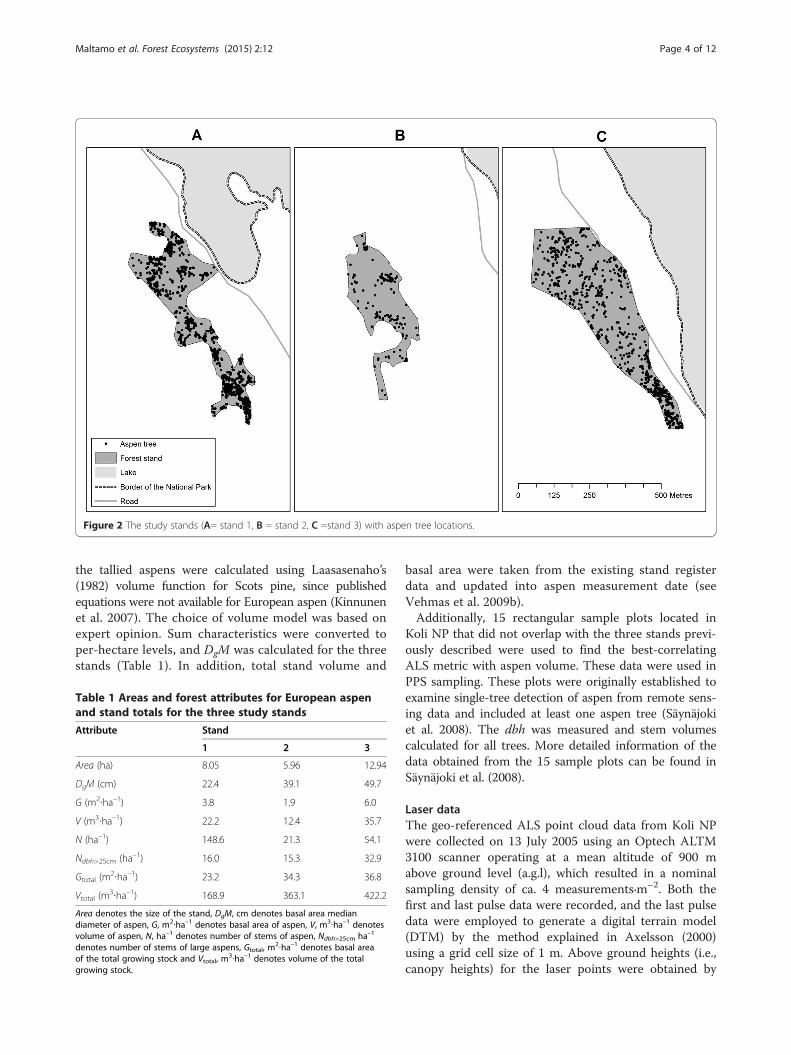
Figure 2 The study stands (A= stand 1, B = stand 2, C =stand 3) with aspen tree locations.


the tallied aspens were calculated using Laasasenaho’s(1982) volume function for Scots pine, since publishedequations were not available for European aspen (Kinnunenet al. 2007). The choice of volume model was based onexpert opinion. Sum characteristics were converted toper-hectare levels, and DgM was calculated for the threestands (Table 1). In addition, total stand volume and

Table 1 Areas and forest attributes for European aspenand stand totals for the three study stands

Attribute Stand

1 2 3

Area (ha) 8.05 5.96 12.94

DgM (cm) 22.4 39.1 49.7

G (m2∙ha–1) 3.8 1.9 6.0

V (m3∙ha–1) 22.2 12.4 35.7

N (ha–1) 148.6 21.3 54.1

Ndbh>25cm (ha–1) 16.0 15.3 32.9

Gtotal (m2∙ha–1) 23.2 34.3 36.8

Vtotal (m3∙ha–1) 168.9 363.1 422.2

Area denotes the size of the stand, DgM, cm denotes basal area mediandiameter of aspen, G, m2∙ha–1 denotes basal area of aspen, V, m3∙ha–1 denotesvolume of aspen, N, ha–1 denotes number of stems of aspen, Ndbh>25cm ha–1

denotes number of stems of large aspens, Gtotal, m2∙ha–1 denotes basal area

of the total growing stock and Vtotal, m3∙ha–1 denotes volume of the total

growing stock.

basal area were taken from the existing stand registerdata and updated into aspen measurement date (seeVehmas et al. 2009b).Additionally, 15 rectangular sample plots located in

Koli NP that did not overlap with the three stands previ-ously described were used to find the best-correlatingALS metric with aspen volume. These data were used inPPS sampling. These plots were originally established toexamine single-tree detection of aspen from remote sens-ing data and included at least one aspen tree (Säynäjokiet al. 2008). The dbh was measured and stem volumescalculated for all trees. More detailed information of thedata obtained from the 15 sample plots can be found inSäynäjoki et al. (2008).

Laser dataThe geo-referenced ALS point cloud data from Koli NPwere collected on 13 July 2005 using an Optech ALTM3100 scanner operating at a mean altitude of 900 mabove ground level (a.g.l), which resulted in a nominalsampling density of ca. 4 measurements∙m–2. Both thefirst and last pulse data were recorded, and the last pulsedata were employed to generate a digital terrain model(DTM) by the method explained in Axelsson (2000)using a grid cell size of 1 m. Above ground heights (i.e.,canopy heights) for the laser points were obtained by


subtracting the DTM at the corresponding location. Inthis study, the pulse data obtained with the ALS sensorwas reclassified to “first echo” or “last echo”. It is worthnoting here that the original single echoes were dupli-cated to both first and last echo classes, whereas theintermediate echoes were completely ignored. For moredetails on the original ALS data, see Vehmas et al.(2009a).The height distribution of the first and last pulse can-

opy height hits was used to calculate plot-wise percen-tiles for 0, 1, 5, 10, 20, …, 90, 95, 99, and 100% heights(h0, h1, …, h100) (Næsset 2004), and cumulative propor-tional crown densities (p0, p1, …, p100) were calculatedfor the respective quantiles. The height distributionscontained only those laser points that were classified asabove-ground hits; a threshold value of 0.1 m was used.The h5, for example, denotes the height at which the ac-cumulation of laser hit heights in the vegetation was 5%,and, correspondingly, p5 denotes the proportion of laserhits that accumulated at the 5% height. In addition, thefollowing variables were calculated by sample plots: thelaser pulse intensities accumulating in percentiles (i10,i30,…, i90), the average intensity value of above-groundhits, the proportion of ground hits versus canopy hitsusing a threshold value of 0.1 m (veg), and the averageheight (hmean) and standard deviation of the above-ground hits (hsd). The intensity values were used as out-putted by the sensor without calibration. All metricswere calculated separately for the first and the last pulsedata.

Stand level inventoryThe methods for aspen inventory were studied based onsimulations using field data from the three stands whereall aspens were mapped. We simulated stand level inven-tory by placing circular plots of size 400 m2 (radius11.28 m) into the stands both systematically and ran-domly. The size of the plot was chosen to correspond tothe grid cell size in PPS sampling (see methodologybelow). Five, ten, fifteen, or twenty plots were located ineach study stand for different sampling intensities. Allsampling alternatives were repeated 2500 times. In thesimulations, plots were only included if the centre pointof the plot was within the study stand. For plots locatedat the edge of the stand, an edge correction was appliedby multiplying the attribute value of an edge plot by itsexpansion factor (Beers 1966):

Attribute ¼ AttributeEdge plot � Plot sizeEdge plot size

ð1Þ

where, attribute is attribute value after correction, attri-buteEdge plot is attribute value of the edge plot, plot size

is size of the sample plot, i.e., 400 m2, and edge plot sizeis the size of the edge plot within the stand.This correction was made for sum attributes V, N, and

Ndbh>25cm but not for DgM. This edge correction isslightly biased but leads to considerably more accurateresults than without applying any correction (Schreuderet al. 1993). Finally, the estimates of forest attributeswere calculated as sample means for each sample.Furthermore, we also tested if the use of ALS data as

auxiliary information would improve the accuracy of thestand level inventory by applying PPS sampling. Thebasic idea of this approach is to use the ALS metric toguide the selection of field plot locations (Pesonen et al.2010a, b). We applied the same number of sample plotsas in the case of systematic and random sampling, butsampling probabilities varied according to ALS informa-tion. This was done to choose the most promising plotlocations for aspen plots. First, probability layers wereproduced, i.e., the auxiliary data values were directlycalculated for the whole stand that was divided into agrid of 20 m × 20 m sample units. When applying PPSsampling, the sample units were square and are referredto as grid cells. ALS based auxiliary data values were cal-culated for each sample unit (i = 1,…, Ngrid, where Ngrid

is the total number of sample units in a stand), andthe probabilities of each unit i being selected weredetermined. The selection probabilities for the sampleunits (pi) were calculated by dividing the auxiliarydata value xi for the sample unit i by the sum of theauxiliary data values over the whole area of the prob-ability layer (pi = xi/∑xi). These selection probabilitieswere finally utilised in sampling 5, 10, 15 or 20 sampleunits. The calculations were repeated 2500 times.

Shape of the diameter distributionIn stands 1 and 3 the shape of the diameter distributionestimated using the simulated fixed-radius, plot-basedinventory approach was compared with the actual em-pirical distribution according to the developed rules. Theunimodal form of diameter distribution (stand 2) wasnot considered. In the comparison of measured and esti-mated diameter distributions, the goal was to examine ifthe sampled distributions followed the underlying actualsize distribution of aspen. The sampled diameter distri-butions were determined in 5- (bimodal stand) or 10-cm(descending stand) diameter classes within the rangefrom 10 − 95 cm (See Figure 3 for actual distributions).For descending diameter distributions, the following rulewas applied:Number of stems in 10–20-cm dbh class > number

of stems in 20–30-cm dbh class > number of stems in30–40-cm dbh class.If this rule was fulfilled by the estimate, it was classi-

fied as a realistic estimate for the underlying empirical

0

100

200

300

400

500

600

10 15 20 25 30 35 40 45 50 55 60 65 70 75 80 85 90 95

Fre

qu

ency

Diameter class midpoint, cm

A

0

5

10

15

20

25

30

10 15 20 25 30 35 40 45 50 55 60 65 70 75

Fre

qu

ency


B

0

20

40

60

80

100

120

10 15 20 25 30 35 40 45 50 55 60 65 70 75 80 85

Fre

qu

ency


C

Figure 3 Diameter distribution of stands 1–3 (A = stand 1, B= stand 2, C =stand 3).


distribution. Correspondingly, in the case of bimodaldistribution, the following rule was applied:The first mode in the distribution is within dbh classes

from 10 − 20 cm, and the second mode in the distribu-tion is after the 25–30-cm dbh class.

Spatial pattern of aspensThe spatial pattern of the aspens within the three studystands was determined by applying Ripley’s K(t) function(Ripley 1981). It describes the expected number of trees

at distance t from a randomly selected tree. If the valueof the function is larger than what would be expectedbased on random spacing, the spatial pattern is clus-tered; if smaller, it is systematic. We applied the libraryspatstat (Baddeley and Turner 2005) in statistical soft-ware R to calculate the K(t) values for each of the threestands. Isotropic correction was applied to minimize edgeeffects in the calculation (Ripley 1988).The spatial patterns derived for the entire stands were

compared with estimates obtained from the simulated


samples. Therefore, a Fisher index (I) was calculated foreach stand-wise simulation obtained using the followingequation:

I ¼ s2n−n; ð2Þ

where s2n is the variance of the plot-wise numbers ofaspens in the sample of 20 plots and �n is the mean ofthe plot-wise numbers of aspens. The I values greaterthan 1 indicate clustered spatial patterns.

Reliability characteristicsThe simulation results were validated in term of relativeRMSE.

RMSE% ¼ 100x

ffiffiffiffiffiffiffiffiffiffiffiffiffiffiffiffiffiffiffiffiffiffiffiffiffiffiffiffiffiffiffiffiffiffi

XNi¼1

y−

Xni¼1

y^i

n

0BBB@

1CCCA

2

N

vuuuuuuut

yð3Þ

and bias

bias% ¼ 100x

XNi¼1

y−

Xni¼1

⌢yi

n

0BBB@

1CCCA

N

yð4Þ

where N is the number of simulations, y is the observedvalue for the stand, ŷi is the predicted value for sampleplot simulation i, and n is number of sample plots inone sample.Finally, in the case of the ALS-guided inventory, the

relative improvement in volume estimate compared toselecting sample units of 20 m × 20 m with equal prob-abilities was calculated.

ResultsReliability figures for attributes of simulated stand levelinventoriesIn general, the results are more accurate by means ofRMSE% when the number of sample plots increases(Table 2). An exception is stand 3 with systematic place-ment of plots where accuracy decreased in the case of20 plots. This is related to the shape of the stand and,thus, to the decreased possibilities to locate the system-atic sample plot network to the narrow, densely stockedsouthern part of the stand in simulations. In general, theresults are also slightly more accurate for systematicthan random plot locations especially in the case of stands

1 and 2. The biases are in most cases below 2% and thereare only a few cases where the values are over 5%.In the case of RMSE% of V, which is usually regarded

as the most important stand attribute, the figures are ra-ther high with smaller number of sample plots and stillremain approximately at the level of 25%–40% even with20 sample plots (Table 2). In stand 2 the RMSE% valueswere larger for V and also for N compared to stands 1and 3. This outcome may be related to the smaller quan-tities of aspen in stand 2 (see Table 1). From the eco-logical point of a view, Ndbh>25cm is the most importantforest attribute. Especially in stand 1, but also in stand 2,most of the aspens had smaller dbh values, less than 25cm (Table 1, Figure 3) and correspondingly the RMSE%figures are high. On the other hand, the RMSE% figuresare lower in stand 3 where the diameter distribution(Figure 3C.) shows that a remarkable proportion of as-pens that reside in the group of trees is in the dbh-classlarger than 25 cm. Finally, in general the results are mostaccurate for DgM.In the case of PPS sampling, the chosen auxiliary in-

formation metric from ALS was hmean2 , which is based

on the correlation estimate (0.76) between aspen V andthis ALS metric in 15 sample plots of Koli NP. Corre-sponding correlations between this ALS metric and gridcell level values in the study area were also calculated,and the effect of the PPS sampling on the reliability of Vestimates in general is presented in Table 3. As shown,the correlation was close to zero in stand 2 and theeffect of PPS sampling is negative in this case. Regardingthe two other stands the correlations between ALS metricand volume were greater than 0.3, and the improvementsin volume estimates were more than 10% and 3%, respect-ively. The minor improvement in stand 3 may be relatedto the existence of very large aspens.

Shape of the diameter distribution estimateThe shape of the diameter distribution of aspen was uni-modal and skewed to the right in stand 2, descending instand 1, and bimodal in stand 3 (Figure 3A–C). Theshape of sample plot based diameter distribution esti-mates obtained from the simulations was examined instands 1 and 3, including ecologically interesting descend-ing and bimodal distributions, respectively. Examinationwas implemented by classifying the diameter distributionestimate of each simulation according to the rules presen-ted in the methods. In stand 1 the proportion of fixed-radius plot estimates, which correctly classified thedescending structure, ranged from 50% − 80% for 5 − 20plots (Table 4). This was the case both for systematicallyand randomly located plots. For stand 3 with a bimodalstructure, the proportion of correctly classified plots withdifferent number of sample plots corresponded to those ofstand 1, but the success rates were lower.

Table 4 Proportion (%) of correctly classified diameterdistribution types in 2500 simulations

Stand Number of plots Inventory method

Systematic Random

Table 2 Relative RMSE and bias (in brackets) values of the forest attributes in three study stands

Stand Sampling rate (%) Sampling alternative Number of plots RMSE (%) (bias %)

V N DgM Ndbh>25cm

1 2.48 Random 5 62.0 (–3.4) 64.3 (–5.0) 56.9 (–10.6) 81.8 (–2.4)

4.97 Random 10 43.8 (–3.3) 45.6 (–2.9) 35.2 (–6.0) 58.2 (–3.5)

7.45 Random 15 35.2 (0.6) 36.2 (0.2) 23.5 (–3.6) 47.7 (–0.5)

9.94 Random 20 30.5 (–1.4) 31.0 (–1.2) 15.5 (–2.1)) 41.8 (–2.1)

Systematic 5 50.8 (–3.0) 56.0 (–4.4) 48.2 (–6.8) 74.3 (–1.2)

Systematic 10 34.5 (–0.1) 40.1 (–1.4) 35.8 (–6.1) 48.5 (0.1)

Systematic 15 25.9 (–2.3) 21.5 (–1.5) 17.8 (–1.8) 49.7 (–4.2)

Systematic 20 24.5 (–1.8) 25.5 (–1.2) 13.5 (–2.5) 38.5 (–2.8)

2 3.36 Random 5 85.7 (–0.2) 83.8 (0) 29.4 (1.3) 87.1 (–0.8)

6.72 Random 10 59.8 (1.2) 59.7 (0.6) 24.5 (–1.4) 60.6 (0.2)

10.08 Random 15 50.0 (–0.2) 49.2 (0) 21.1 (–1.3) 50.1 (–0.2)

13.45 Random 20 41.8 (0.7) 42.7 (–0.6) 18.7 (–0.4) 42.8 (–0.1)

Systematic 5 84.4 (–3.8) 98.2 (–8.2) 28.6 (0.9) 91.9 (–5.9)

Systematic 10 53.2 (0) 47.6 (–2.4) 23.6 (–0.6) 52.2 (–1.4)

Systematic 15 37.6 (1.4) 38.3 (–0.5) 18.5 (–0.3) 42.2 (0.5)

Systematic 20 30.6 (0.1) 31.1 (–0.6) 16.9 (–0.2) 34.6 (–0.3)

3 1.55 Random 5 51.1 (0.2) 64.5 (–0.5) 21.0 (0.5) 52.8 (–0.1)

3.09 Random 10 36.0 (–0.2) 46.3 (–1.8) 13.1 (0.5) 37.7 (–0.7)

4.64 Random 15 29.0 (–0.5) 37.3 (–1.0) 10.1 (–0.1) 30.1 (–0.5)

6.18 Random 20 25.2 (0.1) 31.7 (–0.8) 8.5 (0.1) 25.6 (0.2)

Systematic 5 53.6 (–1.2) 58.4 (2.9) 18.5 (0.5) 52.9 (–0.5)

Systematic 10 33.6 (–0.4) 35.5 (–0.7) 12.8 (–1.6) 36.4 (–0.6)

Systematic 15 26.7 (0) 29.8 (–0.7) 7.7 (–0.2) 24.2 (0)

Systematic 20 33.8 (0.1) 35.7 (0.4) 7.2 (–0.5) 31.9 (–0.2)


Spatial pattern of treesThe analysis based on mapped aspen data with RipleysK-function showed that in all three stands the aspens areclustered, because the expected value of other trees closeto each tree is larger than a Poisson distribution wouldsuggest (Figure 4A–C). Correspondingly, the analysisbased on sampling simulations and Fisher’s index showedthat in each case the average value showed that spatialpattern was clustered (Table 5). Also the proportion ofsimulations showing clustered spatial pattern was alwaysover 50%, even with just five sample plots.

Table 3 Correlation and the improvement in the RMSE ofV (%) due to the use of ALS auxiliary information in PPSsampling

Statistical variable Stand

1 2 3

Correlation 0.35 0.04 0.33

Improvement in the RMSE of V (%) 10.6 –7.0 3.2

DiscussionThis study considered stand level aspen populations in aboreal nature reserve. The analysis was based on diam-eter distribution, spatial pattern of aspen trees and reli-ability figures of forest attribute estimates of stand levelinventory. Our unique data included mapped aspen trees

1 5 51.2 54.9

10 65.4 66.9

15 76.0 75.0

20 78.8 78.6

3 5 35.3 36.7

10 52.2 49.9

15 55.2 54.7

20 65.1 61.7

Figure 4 Ripley’s K function for stands 1–3 (A= stand 1, B = stand 2, C =stand 3). The dashed line describes the expected value of trees basedon Poisson distribution with radius r, and solid line the estimate obtained using Ripley’s K function and isotropic edge correction.


in three spruce dominated forest stands where localaspen populations have survived during the past 100years (Vehmas et al. 2009b). These stands also representfavourable growing environments of aspen. The propor-tion of aspen in these stands is considerably higher thanthe average value of 1.5% in Finland (Tomppo et al. 2001)being 16.3%, 5.5% and 16.2% of basal area in stands 1, 2and 3, respectively. These statistics are for the forest areain general, but in conservation areas the proportion of

aspen is usually considerably larger. It also should benoted that our study stands were rather large in size com-pared to the average stand size, which is ca. 2 ha in south-ern Finland. However, with respect to the state-ownedforests and conservation areas where aspen is common,the stand sizes used in this study were broadly similar.The acceptable level of forest attribute results is, of

course, dependent on the need for information, butaccording to inventory by compartments, the RMSE

Table 5 Average values of Fisher index and proportion ofclustered spatial patterns of aspen trees in 2500simulations

Stand Numberof plots

Random Systematic

Average Proportionof clusteredsamples

Average Proportionof clusteredsamples

1 5 8.6 94.1 9.5 96.1

10 9.9 99.6 10.0 99.2

15 10.0 100.0 11.4 100.0

20 10.6 100.0 10.6 100.0

2 5 1.9 56.1 2.0 60.4

10 2.3 73.4 2.6 84.1

15 2.6 84.5 2.7 90.9

20 2.7 90.2 2.8 95.6

3 5 3.0 94.1 3.1 96.1

10 3.5 95.6 3.7 89.8

15 3.7 95.6 4.1 98.7

20 3.9 98.0 4.0 97.0


values of V for deciduous tree species in mixed standsshould be between 20% − 50% in Finnish conditions(Uuttera et al. 2002). However, in the previous studiesthe RMSE% figures have been higher (65%) for decidu-ous tree species (birches) (Haara and Korhonen 2004).Our results showed, in general, that with the lower num-ber of sample plots the RMSE figures are over 50% butthe requirement set by Uuttera et al. (2002) is possibleto obtain by measuring 10 or more plots. Between thethree stands, the differences in accuracy were caused bythe amount of aspen growing stocks, the sizes of thestands (i.e., sampling intensity) and small differences inthe spatial patterns of trees. The effect of these aspectsis to some extent inversely related. For example, in stand2, the sampling intensity was highest, but also the RMSEfigures were still the highest. This is most likely due tothe low amount of aspen in the growing stock.We also guided random sample plot placement by

applying auxiliary ALS information with PPS sampling.This kind of approach previously has been applied instudies by Pesonen et al. (2010a, b) in the estimation ofquantities of coarse woody debris (CWD). The chosenALS metric, the square of the mean height of laserechoes emphasized the grid cells with the tallest trees. Inour case, this technique decreased sampling efficiency instand 2. This was due to the negative correlation be-tween aspen volume and the square of the mean heightof laser, i.e. the tallest trees in stand 2 are not aspens.This can be considered a drawback of the approach. Ifpre-information concerning the chosen variable does nothold true, the benefit is completely lost. In our case, thecorrelation between aspen volume and ALS metric-derived

mean height was very strong in the 15 large sized fixed-area aspen sample plots, which were earlier used in singletree-based aspen detection from ALS data in the same Koliarea (Säynäjoki et al. 2008), but obviously this kind of infor-mation cannot be generalised without risks associated withthe extrapolation.With respect to aspen populations in conservation

areas, the detailed information on diameter distribution(e.g., the number of large aspens and the shape of distri-bution) is also of primary interest because many aspen-associated species are highly specialised to specific treeproperties (Kouki et al. 2004; Sahlin and Ranius 2009).While descending diameter distribution shapes are inter-preted as indicators of uneven-aged stand structure and,thus, may reflect the continuity of aspen populations,bimodal distributions reveal the existence of more thanone aspen layer, which is usually also strongly related tothe stand age structure. Information on both of thesedistribution types can be utilised in the management ofconservation areas, and without this information, themanagement lacks primary attributes characterising stands.Regarding our results on mimicking distribution types with10 fixed-radius plots, the proportions of correctly describeddiameter distributions were about 65% and 50% whenobtained for the descending and bimodal diameter distri-butions, respectively. These proportions can be furtherincreased more than 10 percentage units by increasing thenumber of sample plots. The same trend is also true forNdbh>25cm, 10 or more measured sample plots may be re-quired to reach the 25%–50% level of RMSE%.During the last fifteen years, numerous field-based

sampling methods for assessing different sparse popu-lations have been presented (e.g. Holopainen et al. 2006;Ringvall et al. 2007; Gove et al. 2013). Although aspenpopulations are sparse in general this is not the case inour study data. The abundance of aspen in our stands iscomparable to the abundance of birch in Finland whichconstitutes 17% of growing stock and is the third mostfrequent tree species of the country (Metsätilastollinenvuosikirja 2013). In such conditions the use of sparsepopulation inventory methods may lead to high cost andtime-consuming fieldwork. Since there are numeroussampling methods for sparse populations, the suitabilityof some of these, such as parallel strips suggested byMarquardt et al. (2012), could be investigated for ourdata that is, in any case, a topic for future studies.According to the analysis of spatial patterns, the as-

pens were strongly clustered in all three stands. This isin line with previous findings (e.g. Syrjänen et al. 1994).In general clustered spatial patterns of trees make inven-tory more challenging (Pippuri et al. 2012) which is con-sistent with the RMSE% levels of our study. On the otherhand, it is worth noting that the clustered spatial patternof aspens was also successfully identified from sample


plots without the information of tree location. This is animportant outcome for planning aspen inventories.In our study, remote sensing was only applied as auxil-

iary information in PPS sampling. However, in earlierstudies, individual aspens have been detected from ALSdata or they have been part of tree stock descriptions inarea-based approaches. The problems related to single-tree detection include the typically very low general de-tection rate and overlapping of aspen intensity valueswith other tree species, such as birch and pine. Also, thevast size of the crown of mature aspen trees would even-tually cause difficulties for interpretation when crownsizes of other trees were considerably smaller. On theother hand, when successful, single-tree detection wouldreveal unforeseen information on aspen crowns. Here,we did not apply single-tree detection, since the techniquewas already tested with data from Koli NP by Säynäjokiet al. (2008). In the case of ABA, earlier studies haveshown poor accuracy estimates obtained for aspen. In ourcase, this approach was inapplicable, since the number ofmeasured training plots available in Koli NP was not ad-equate and the forest vertical structure and tree speciesconstitution outside Koli NP is considerably different.

ConclusionsThis study characterized European aspen populations forthe purposes of monitoring and management of borealconservation areas. Our results suggest that if the num-ber of sample plots is adequate, i.e. 10 or more usingplot size 400 m2, stand level inventory will provide ac-curate enough forest attributes estimates in conservationareas (minimum accuracy requirement of RMSE% is20%–50%). Even for the more ecologically valuableattributes, such as diameter distribution, spatial patternand large aspens, the estimates are acceptable for conser-vation purposes. Between the three stands, the differencesin accuracy were caused by the amount of aspen growingstocks, the sizes of the stands and small differences in thespatial patterns of trees. ALS-based auxiliary informationmight also be useful in guiding the inventory. However,there is still the major risk that relying on ALS may de-crease accuracy. Completely remote sensing-based inven-tory applications for such detailed attributes obtainablefor aspens must still await further development of sensorsand algorithms, such as multispectral ALS or combinationof ALS and hyper spectral data.

Competing interestsThe authors declare that they have no competing interests.

Authors’ contributionsMM participated to all phases of the study. AP calculated the resultsconcerning sampling simulations and participated to writing ofcorresponding parts of the study. LK calculated the results concerning spatialpattern of trees and participated to writing of corresponding parts of thestudy. JK was responsible of the ecological part of the Background and

Discussion. MV conducted fieldwork and ALS metrics analysis. KE participatedplanning and writing of the study. All authors have read and commentedthe manuscript. All authors read and approved the final manuscript.

AcknowledgementsThis work was supported by by the strategic funding of the University ofEastern Finland. We thank Ms Anne Nylander for her help with the compilationof the figures.

Author details1University of Eastern Finland, School of Forest Science, P.O. Box 111,FI-80101 Joensuu, Finland. 2Blom Kartta Oy, Kauppakatu 15, 80100 Joensuu,Finland. 3City of Joensuu, 80100 Joensuu, Finland. 4Natural ResourcesInstitute Finland, Joensuu Unit, P.O. Box 68, FI-80101 Joensuu, Finland.

Received: 15 December 2014 Accepted: 17 April 2015

ReferencesAxelsson P (2000) DEM generation from laser scanner data using TIN models.

In: The International Archives of the Photogrammetry and Remote Sensing,vol 33, Part B4/1, Amsterdam, pp 110 − 117

Baddeley A, Turner R (2005) Spatstat: an R package for analyzing spatial pointpatterns. J Stat Soft 12:1–42

Beers TW (1966) The direct correction for boundary-line slopover in horizontalpoint sampling. Research Progress Report 224, Purdue University,Agricultural Experiment Station, Lafayette, Indiana, p 8

Breidenbach J, Næsset E, Lien V, Gobakken T, Solberg S (2010) Predictionof species-specific forest inventory attributes using a nonparametricsemi-individual tree crown approach based on fused airborne laser scanningand multispectral data. Remote Sens Environ 114:911–924

Esseen PA, Ehnström B, Ericson L, Sjöberg K (1992) Boreal forests—the focalhabitats of Scandinavia. In: Hansson L (ed) Ecological Principles of NatureConservation. Elsevier Applied Science, London

Gove JH, Ducey MJ, Valentine HT, Williams MS (2013) A comprehensivecomparison of perpendicular distance sampling methods for samplingdowned coarse woody debris. Forestry 86:129–143

Grönlund A, Hakalisto S (1998) Management of traditional rural landscapes in KoliNational Park. Separate plan of Koli National Park. North Karelia RegionalEnvironment Centre, Joensuu, Regional environmental publications104, pp 81

Haara A, Korhonen KT (2004) Kuvioittaisen arvioinnin luotettavuus. Metsätieteenaikakauskirja 4(2004):489–508

Heliövaara K, Väisänen R (1984) Effects of modern forestry on northwesternEuropean forest invertebrates: a synthesis. Acta For Fenn 189:1–32

Holopainen M, Leino O, Kämäri H, Talvitie M (2006) Drought damage in the parkforests of the city of Helsinki. Urban For Urban Gree 4:75–83

Kalliola R (1973) Suomen kasvimaantiede. Werner Söderström Osakeyhtiö, PorvooKärkkäinen S (1994) Herb-rich forest vegetation of the Koli area. Publication of

the Water and Environment Administration: series A 172, pp 51Kinnunen J, Maltamo M, Päivinen R (2007) Standing-volume estimates of forests

in Russia: how accurate is the published data? Forestry 80:53–64Koivuniemi J, Korhonen KT (2006) Inventory by compartments. In: Kangas A.,

Maltamo M. (eds) Forest Inventory. Methodology and Applications. ManagingForest Ecosystems, vol 10, Springer, Dordrecht, pp 271–278

Korpela I, Ørka H-O, Maltamo M, Tokola T, Hyyppä J (2010) Tree speciesclassification in airborne LiDAR data: influence of stand and tree factors,intensity normalisation, and sensor type. Silva Fenn 44:319–339

Kouki J, Arnold K, Martikainen P (2004) Long-term persistence of aspen, a keyhost for many threatened species, is endangered in old-growth conservationareas in Finland. J Nat Conserv 12:41–52

Kurkela T (1973) Epiphytology of Melampsora rusts of Scots pine (Pinus sylvestris L.)and aspen Populus tremula L. The Finnish Forest Research Institute ResearchReport 79, pp 68

Laasasenaho J (1982) Taper curve and volume functions for pine, spruce, andbirch. Commun Inst For Fenn 108:74

Lilja S, Wallenius T, Kuuluvainen T (2006) Structural characteristics and dynamicsof old Picea abies forests in northern boreal Fennoscandia. EcoScience13:181–192

Lyytikäinen A (1991) Kolin luonto, maisema ja kulttuurihistoria. Kolinluonnonsuojelututkimukset. Vesi- ja ympäristöhallituksen monistesarja 308


Maltamo M, Packalen P (2014) Species-specific management inventory in Finland.In: Maltamo M, Naesset E, Vauhkonen J (eds) Forestry Applications ofAirborne Laser Scanning: Concepts and Case Studies. Managing ForestEcosystems, vol. 27th edn. Springer, Dordrecht, pp 241–252

Marquardt T, Temesgen H, Eskelson BNI, Anderson P (2012) Evaluation ofsampling methods to quantify abundance of hardwoods and snags withinconifer dominated riparian zones. Ann For Sci 69:821–828

Metsätilastollinen vuosikirja (2013) http://www.metla.fi/julkaisut/metsatilastollinenvsk. Accessed 20 Dec 2013

Næsset E (2004) Practical large-scale forest stand inventory using asmall-footprint airborne scanning laser. Scand J For Res 19:164–179

Næsset E (2007) Airborne laser scanning as a method in operational forestinventory: status of accuracy assessments accomplished in Scandinavia.Scand J For Res 22:433–442

Ørka HO, Næsset E, Bollandsås OM (2007) Utilising airborne laser intensity for treespecies classification. In: International Archives of the Photogrammetry,Remote Sensing, and Spatial Information Sciences, vol 36, Part 3/W52,pp 300–304

Packalén P, Maltamo M (2007) The k-MSN method in the prediction ofspecies-specific stand attributes using airborne laser scanning and aerialphotographs. Remote Sens Environ 109:328–341

Pesonen A, Kangas A, Maltamo M, Packalén P (2010a) Different sources ofauxiliary information in coarse woody debris inventory. Forest Ecol Manag259:1890–1899

Pesonen A, Maltamo M, Kangas A (2010b) The comparison of airborne laserscanning-based probability layers as auxiliary information for assessing coarsewoody debris. Int J Remote Sens 31:1245–1259

Pippuri I, Kotamaa E, Maltamo M, Peltola H, Packalén P (2012) Exploringhorizontal area-based metrics to discriminate the spatial pattern oftrees and need for first thinning using airborne laser scanning.Forestry 85:305–314

Pippuri I, Maltamo M, Packalen P, Mäkitalo J (2013) Predicting species-specificbasal areas in urban forests using airborne laser scanning data and existingstand register data. Eur J For Res 132:999–1012

Poso S (1983) Basic features of forest inventory by compartments. Silva Fenn17:313–349

Ringvall A, Snäll T, Ekström M, Ståhl G (2007) Unrestricted guided transectsampling for surveying sparse species. Can J For Res 37:2575–2586

Ripley BD (1981) Spatial statistics. John Wiley & Sons, New YorkRipley BD (1988) Statistical inference for spatial processes. Cambridge University

Press, CambridgeSahlin E, Ranius T (2009) Habitat availability in forests and clearcuts for saproxylic

beetles associated with aspen. Biodivers Conserv 18:621–638Säynäjoki R, Packalén P, Maltamo M, Vehmas M, Eerikäinen K (2008) Detection of

aspens using high-resolution aerial laser scanning data and digital aerialimages. Sensors 8:5038–5055

Schreuder HT, Gregoire TG, Wood GB (1993) Sampling Methods for MultiresourceForest Inventory. John Wiley & Sons, New York

Stokland JN, Holien H, Gaarder G (2002) Arealtall for boreal regnskog i Norge2002. NIJOS-rapport 2:1–20

Syrjänen K, Kalliola R, Puolasmaa A, Mattson J (1994) Landscape structure andforest dynamics in sub-continental Russian European taiga. Ann Zoo Fenn31:19–34

Tikka PS (1954) Structure and quality of aspen stands. I. Structure. Commun InstFor Fenn 44:1–33

Tomppo E, Henttonen H, Tuomainen T (2001) Valtakunnan metsien 8.inventoinnin menetelmä ja tulokset Metsäkeskuksittain Pohjois-Suomessa1992–94 sekä tulokset Etelä-Suomessa 1986–92 ja koko maassa 1986–94.Metsätieteen aikakauskirja B/2001: 99–248

Uuttera J, Hiltunen J, Rissanen P, Anttila P, Hyvönen P (2002) Uudet kuvioittaisenarvioinnin menetelmät– Arvio soveltuvuudesta yksityismaidenmetsäsuunnittelu. Metsätieteen Aikakauskirja 3(2002):523–531

Vehmas M, Eerikäinen K, Peuhkurinen J, Packalén P, Maltamo M (2009a) Airbornelaser scanning-based identification of herb-rich mature forests in the KoliNational Park, eastern Finland. Forest Ecol Manag 257:46–53

Vehmas M, Kouki J, Eerikäinen K (2009b) Long-term spatiotemporal dynamics andhistorical continuity of European aspen (Populus tremula L.) stands in KoliNational Park, eastern Finland. Forestry 82:135–148

Submit your manuscript to a journal and benefi t from:

7 Convenient online submission

7 Rigorous peer review

7 Immediate publication on acceptance

7 Open access: articles freely available online

7 High visibility within the fi eld

7 Retaining the copyright to your article

Submit your next manuscript at 7 springeropen.com

http://www.metla.fi/julkaisut/metsatilastollinenvsk

http://www.metla.fi/julkaisut/metsatilastollinenvsk

inventory of aspen trees in spruce dominated stands in

Documents