Image completion by diffusion maps and spectral relaxation

Shai Gepshtein∗, Yosi Keller†

Abstract

We present a framework for image inpainting based on the Diffusion Framework. By choosing

appropriate diffusions kernels and image affinity measures, the corresponding Diffusion embedding

is shown to be smoother than the source image and can thus be inpainted by simple exemplar-based

and variational methods. We discuss the properties of the induced smoothness and relate it to the

underlying assumptions used by previous inpainting schemes. As the Diffusion embedding in non-

linear and non-invertible, we propose a novel computational approach to computing an approximate

mapping from the embedding space to the image domain. We formulate the mapping as a discrete

optimization problem, solved via spectral relaxation. As the embedding space provides a canonical

smooth representation, our approach can inpaint both textured and smooth images. The effective-

ness of the presented method is exemplified by inpainting real images, and comparisons to previous

state-of-the-art schemes.

1 Introduction

Image inpainting algorithms aim to fill the missing data of an image or a video sequence in a visually

plausible way, such that the insertion is not easily detectable by a common unsuspecting viewer. Thus,

this problem lies at the intersection of computer graphics, image, and signal processing. Formally,

given a corrupted image I and a “hole” region mask H marking the unknown area, the goal of image

completion is to fill in H to form a visually plausible image I. This is depicted in Fig. 1a.

The problem has attracted significant research effort, and existing methods can be categorized as

being either exemplar-based or variational schemes. Variational schemes [1, 2, 3, 4] formulate the

∗Faculty of Engineering, Bar Ilan University, Israel. shaigep@gmail.com.†Faculty of Engineering, Bar Ilan University, Israel. yosi.keller@gmail.com.

1

inpainting as the minimization of a variational functional that encodes spatial smoothness constraints.

The minimizations of such functionals results in the solution of linear or nonlinear heat equations. Thus,

these schemes assume that the inpainted images contain piecewise smooth spatial manifolds. Exemplar-

based schemes [5, 6, 7, 8] implicitly assume that H can be inpainted by replicating image patches given

in a reference set H, that might consist of the known parts of the input image I = H∪H, or a given set of

images [9, 10]. Such schemes were proven to provide efficient solutions, but lack the global optimality of

the variational approaches. A combination of these two classes of methods were also proposed utilizing

both global geometric completion and texture synthesis [11, 12].

(a) (b) (c) (d)

Figure 1: (a) Source image to be inpainted. (b) The source image inpainted by an isotropic heat equation.

(c) The leading eigenvectors inpainted using an isotropic heat equation (d) The image inpainted by

computing the inverse Diffusion mapping of (c).

In this work, we propose a new image inpainting framework where the completion algorithm is

executed in a diffusion map feature space [13]. Each pixel xi j ∈ I in the reference set H is represented

by a patch pi j ∈ RD, thus forming the reference set

pi j

, where D is typically 5× 5 or 7× 7. To

analyze this high dimensional data set, we use diffusion maps for dimensionality reduction. Thus, we

implicitly assume that the unknown image patches pi j ∈ H and the patches in the reference set pi j ∈ H

belong to the same low dimensional manifold, parameterized by the diffusion kernel. The dimensionality

reduction is feasible due to the low intrinsic dimensionality of the image patches, manifested by their

local correlations [14]. Using the embeddings, patches are mapped into a low dimensional space

H 7−→ Ψ(H),Ψ ∈ Rd, d << D (1)

This is shown in Fig. 1, where a textured image contains a rectangular hole H to be filled. Applying

2

a variational inpainting scheme might result in excessive smoothing (Fig. 1b). However, using dif-

fusion maps to reduce the dimensionality of the data, the resulting embedding (eigenvectors) shown

in Fig. 1c, is smooth. Due to this smoothness, the holes in the ’images’ of the eigenvectors can

be inpainted using simple interpolation methods. As the Diffusion embedding is nonlinear, and non-

invertible, the missing data in the image domain cannot be computed directly. For that, we derive a

novel approximate embedding inversion scheme that assigns an image patch pi j ∈ H to each inpainted

point yi j ∈

ψk1(xi, j)...ψkm(xi, j)T in the embedding domain. The assignment problem is solved via

spectral relaxation [15] and induces spatial regularization.

Thus, we provide two core contributions: First, a general framework for data completion by de-

riving smooth representations via Diffusion embedding. In particular, it provides a unified scheme to

inpainting textured and textureless images. Second, we derive a scheme for approximating the inverse

of the Diffusion embedding and map the interpolated embeddings back to the data/image domain, by

formulating the inverse-mapping as an assignment problem, that optimizes a global smoothness con-

straint. The solution to the resulting combinatorial problem is NP-hard, and is efficiently approximated

by spectral relaxation.

The framework we present is general in nature and can be applied to many data sources of interest

such as audio signals and tabular data. Yet, in this work we chose to concentrate on the image inpainting

problem that provides an intuitive testbed for data embedding and a baseline of previous state-of-the-art

works to compare against.

This paper is organized as follows: we start by reviewing previous works on image inpainting in Sec-

tion 2.1 and recalling the diffusion framework in Section 2.2. The proposed image inpainting schemes

is introduced and discussed in Section 3. It is experimentally verified and compared with existing ap-

proaches in Section 4. Concluding remarks are discussed in Section 5.

2 Background

In this section we survey previous results in image inpainting (Section 2.1) and provide background on

the Diffusion Maps (Section 2.2) that is the main computational tool used in our work.

3

2.1 Image inpainting

The study of image inpainting lies at the intersection of image processing and computer graphics. Thus,

the fundamentals of many contemporary inpainting schemes can be traced back to the seminal contribu-

tions of Efros and Leung [5] (exemplar-based) and Bertalmıo [1] et al. (variational schemes).

Exemplar based techniques proved to be successful in dealing with large-scale image completion

tasks (note the Bungee example in Fig. 14). Such methods fill the missing pixels by copying source

patches from the observed part of the image to produce plausible visual results. Texture synthesis by

non-parametric sampling was first introduced by Efros and Leung [5] that proposed a greedy scheme

that operates on the pixels of the boundary ∂H, and successively fills the hole towards its center. The

most similar patch (in terms of the L2 norm) in I is found and copied as the predicted new value. Such

schemes are sensitive to the filling order, and might propagate errors of wrongly selected filling pixels,

leading to visual inconsistencies.

Criminisi et al. [6] extended the previous scheme by introducing priority ordering to derive the

order in which the pixels are synthesized. The ordering is given by two terms. The first quantifies the

strength of the isophotes hitting the hole’s border, thus encouraging linear structures with high strength

of isophotes to be synthesized first. The second encodes the reliability of the information in the pixel’s

vicinity. Therefore, patches that have more of their neighboring pixels already filled will be filled first.

The priority assignment is a product of the two terms computed at each pixel and updated in each

iteration of the algorithm.

A globally optimal formulation of exemplar based inpainting was suggested by Wexler et al. [7],

where the objective function adds a constraint that missing pixels have to be consistent with all the

surrounding patches forming them. In order to reach a global optimum, the inpainting is iterated until the

update converges. This approach utilizes a multi-scale formulation by initiating the iterative completion

at the coarsest level of the pyramid, and propagating the result upward. This allows improved global

consistency and speeds up the convergence. The authors extended this approach [7] by introducing

spatial and temporal constraints for video inpainting via a variational formulation.

Another iterative exemplar based scheme was suggested by Drori et al. [8], where the unknown

region is approximated by classifying the pixels to an underlying structure that agrees with other parts

of the image. The approximated region is then augmented with details extracted from high confidence

4

regions. The scheme is iterated in different scales until convergence.

The computational bottleneck of exemplar-based schemes is the search for the patch most similar

to the one being inpainted, as this search is repeated at each iteration. Barnes et al. [16] proposed

an efficient approach to K-nn search of image patches, denoted as Patchmatch that provides an order

of magnitude performance improvement over previous state-of-the-art schemes such as KD-trees. Their

approach is based on random initiation of the patch matches followed by the propagation of patches in the

vicinity of well matched patches. It was successfully applied to applications such as image inpainting,

retargeting and reshuffling.

The focal point of variational schemes is to formulate the inpainting problem as the minimization

of variational functionals. Using the calculus of variations, the minimization of such functionals boils

down to the solution of a nonlinear PDEs [1], where the pixels on the boundary ∂H, are used as boundary

conditions. Thus, image information is propagated from ∂H into the hole H. The propagation is gov-

erned by the chosen functional and the resulting PDE, where nonlinear anisotropic diffusion is preferred

to isotropic diffusion as it avoids over smoothing. Some schemes [2, 17] propose to directly choose a

PDE with desirable inpainting properties, without deriving it by the minimization of a functional and

are thus non-variational. Such schemes were shown to be beneficial when inpainting piecewise smooth

images or when the hole H is relatively narrow. Yet, they might fail when inpainting the textured parts

of an image.

One of the first schemes utilizing the propagation approach was suggested by Masnou et al. [18],

that inpaint by joining points of level lines arriving at the boundary of H with geodesic curves. The

edges recovered by this approach are smooth and continuous at the boundary of the hole, and it shows

good results for inpainting thin holes. A combination of variational and exemplar based methods was

proposed by Bertalmio [12] and Bugeau [11]. The algorithm combines texture synthesis and geometric

methods for image inpainting through structure-texture decomposition. Bugeau [11] applied PDE-based

techniques to the structure image that is smoother than the original one, and encodes the high frequencies

of the image.

Tschumperle and Deriche [17] proposed a general framework for vector-valued image regulariza-

tion, that is based on variational methods and PDEs. They derive local filters based on anisotropic

diffusion. The approach is shown to be applicable to a class of image processing tasks such as image

5

magnification, restoration and inpainting. An image inpainting scheme that combines exemplar-based

and PDE-based approaches was suggested by Le Meur et al. [19]. The structure tensor is used to set the

filling order in the isophote direction, while the optimal image patch used to inpaint the hole, is found

via template matching.

An inpainting scheme based on discrete optimization was suggested by Komodakis et al. [20],

where a discrete variational-like functional is iteratively minimized using priority-belief propagation.

The scheme solves a global discrete optimization over all possible patches, using dynamic label-pruning

to significantly reduce the number of labels. A different class of recent results is based on sparse recon-

struction [21, 22], where an image is represented as a set of image patches that are processed as a set of

high dimensional samples for which a sparse dictionary is learnt. The missing data H is extrapolated by

linear combinations of the dictionary atoms, computed via L1 minimization.

Our work relates to both variational and sparse reconstruction based approaches, as these assume

that the inpainted image belongs to a low-dimensional space, being either the space of smooth images

(as in the variational approaches) or in the space spanned by a sparse dictionary. Our scheme utilizes a

different notion of low dimensionality and smoothness that relates to the Diffusion Framework [13]. By

utilizing application-specific affinity measures and kernels (Section 3.3) we induce a chosen smoothness

over the image manifold. Thus, simple variational approaches can be applied to inpaint textured images.

These different notions of smoothness are further discussed in Section 3.4.

2.2 Diffusion maps

In this Section we survey the diffusion framework, where a broader view can be found in [13, 14]. Given

a set X = x1, ...,xn of n data points, such that xi ∈ RD. Our goal is to compute a set Y = y1, ...,yn,

where yi ∈ Rd , such that yi represent xi. Such representation forms a low dimensional mapping of the

data points if d ≪ D.

The core of the Diffusion framework is to represent the input dataset X by an undirected graph

G = (V,E) with nodes V = x1, ...,xn, and edges that quantify the affinity between two “close” points

xi and x j, such that E ∈wi, j. The affinity wi, j is required to be symmetric, non-negative and is commonly

computed using a RBF kernel

wi, j = exp(−∥xi −x j∥2/σ2) = exp(−di j2/σ2) (2)

6

where σ > 0 is a scale parameter. σ is a measure of closeness that may prune edges from the graph such

that two points xi and x j will have nonzero affinity wi, j if their distance di j < 3σ. This weight is related

to the heat kernel and defines the nearest neighbor structures of the graph.

The computation of wi, j is application-specific. In images, the distance di j is chosen to encode

different image attributes such as color spaces (RGB, LAB), texture via texture descriptors (such as

LBP), and low-level image structures (edges). This is further discussed in the context of our work

in Section 3.3. Coifman and Lafon [13] proved that any weight of the form h(∥xi − x j∥) allows to

approximate the heat kernel if h decays sufficiently fast at infinity, and this justifies the use of the RBF

kernel in Eq. 2. The core of the diffusion framework is to induce a random walk on the data set X by

normalizing the weights to a Markov matrix

A = D−1W (3)

where dii = ∑ j wi, j is the degree of node xi. A is row stochastic and can be viewed as a random walk

process as ai, j ≥ 0 and ∑ j ai, j = 1. The term ai, j represents the probability to jump from xi to x j in a

single time step. The corresponding matrix A ∈ Rn×n represents the transitions of this Markov chain in

a single step

atik = Pr(x(t) = xk | x(0) = xi). (4)

A encodes a time-homogeneous Markov chain, and taking powers of this matrix amounts to running

the chain forward in time. At represents the probabilities of transition from xi to x j in t time steps. If

the graph is connected, the stationary distribution that satisfies the equation ϕT0 A = ϕT

0 is also the left

eigenvector of the transition matrix A associated with the eigenvalue λ0 = 1.

The observation of the weights as probabilities of a random walk process paves the way for a spectral

decomposition scheme. The eigendecomposition of the transition matrix with respect to the Markovian

time variable t yields

At(xi,x j) = ∑l≥0

λtlψl(xi)ϕl(x j) , (5)

where λl is the sequence of eigenvalues of A (with λ0 = 1) and ϕl and ψl are the corresponding

biorthogonal left and right eigenvectors. Due to the spectrum decay, only a few terms are needed to

achieve a given relative accuracy in Eq. 5.

7

The diffusion distance quantifies the similarity between two points xi and x j by their probability

distributions

D2t (xi,x j) = ∑

k∈Ω

(atik −at

jk)2

ϕ0(k). (6)

This quantity is a weighted L2 distance between the conditional probabilities atik and at

jk, that can be

thought of as features measuring the interaction of the nodes xi and x j with the rest of the graph. The

relation between the diffusion distance and the eigenvectors is given by

D2t (xi,x j) = ∑

l≥1λ2t

l (ψl(xi)−ψl(x j))2 (7)

This identity implies that the right eigenvectors can be used to compute the diffusion distance, where

the different eigenvectors are weighted by the corresponding eigenvalues λl, and only a few terms are

needed to achieve a given relative accuracy in Eq. 7 due to the spectrum decay.

Hence, the right eigenvectors ψl can be used as a new set of coordinates for the set X , such that

the Euclidean distance between these Diffusion coordinates ψl approximates the diffusion distance in

Eq. 7. Let d(t) be the number of terms retained, the diffusion map (embedding) is given by

Ψt : x 7−→(

λt1ψ1(x),λt

2ψ2(x), . . . ,λtd(t)ψd(t)(x)

)T. (8)

Using the diffusion map, we represent a graph of any generic data set as a cloud of points in a Euclidean

space, where the chosen affinity measure allows to quantify a particular, application-specific distance

measure.

3 Image completion

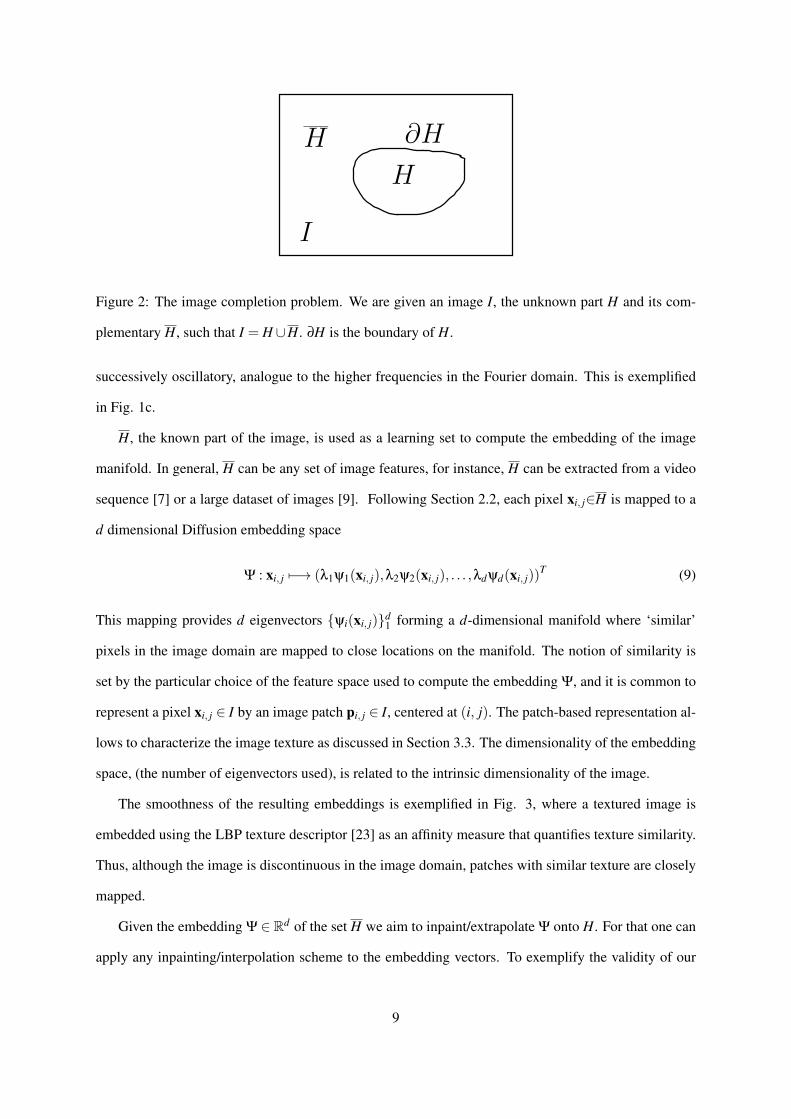
Let I be an image consisting of an unknown part H and its complementary H, and let ∂H be the boundary

of H. We aim to inpaint H by extending the boundary values I (∂H) into H, as depicted in Fig. 2.

The core of our approach is to represent the image in the Diffusion space discussed in Section 2.2,

and inpaint the embedding, instead of inpainting the pixel values as in previous works. By choosing

an appropriate similarity measure between the pixels xi ∈ H, the embedding can be made smooth, thus

allowing simple inpainting in the Diffusion domain. The spatial smoothness of the embedding vectors

stems from them being the eigenvectors of a Sturm–Liouville operator, where similar to the Fourier do-

main, the leading eigenvector is the smoothest, constant vector, and the following eigenvectors become

8

H

H

I

∂H

1

Figure 2: The image completion problem. We are given an image I, the unknown part H and its com-

plementary H, such that I = H ∪H. ∂H is the boundary of H.

successively oscillatory, analogue to the higher frequencies in the Fourier domain. This is exemplified

in Fig. 1c.

H, the known part of the image, is used as a learning set to compute the embedding of the image

manifold. In general, H can be any set of image features, for instance, H can be extracted from a video

sequence [7] or a large dataset of images [9]. Following Section 2.2, each pixel xi, j∈H is mapped to a

d dimensional Diffusion embedding space

Ψ : xi, j 7−→ (λ1ψ1(xi, j),λ2ψ2(xi, j), . . . ,λdψd(xi, j))T (9)

This mapping provides d eigenvectors ψi(xi, j)d1 forming a d-dimensional manifold where ‘similar’

pixels in the image domain are mapped to close locations on the manifold. The notion of similarity is

set by the particular choice of the feature space used to compute the embedding Ψ, and it is common to

represent a pixel xi, j ∈ I by an image patch pi, j ∈ I, centered at (i, j). The patch-based representation al-

lows to characterize the image texture as discussed in Section 3.3. The dimensionality of the embedding

space, (the number of eigenvectors used), is related to the intrinsic dimensionality of the image.

The smoothness of the resulting embeddings is exemplified in Fig. 3, where a textured image is

embedded using the LBP texture descriptor [23] as an affinity measure that quantifies texture similarity.

Thus, although the image is discontinuous in the image domain, patches with similar texture are closely

mapped.

Given the embedding Ψ ∈ Rd of the set H we aim to inpaint/extrapolate Ψ onto H. For that one can

apply any inpainting/interpolation scheme to the embedding vectors. To exemplify the validity of our

9

Figure 3: An image and its embedding. Patches with similar texture are mapped to close locations on

the manifold, using an embedding based on LBP texture descriptors [23].

approach, we chose to use a simple linear isotropic diffusion

φi = 0, φi (∂H) = ψi (∂H) . i = 1..d (10)

Equation 10 is applied to each eigenvector ψi separately, and while this approach is inferior to using

multidimensional nonlinear variational schemes, it emphasizes the simplicity of the inpainting problem,

as formulated in the embedding domain. We also applied Criminisi’s exemplar based approach [6] in

the embedding domain to compare against the isotropic interpolation.

Having computed the extrapolated embedding coordinates φi(xi, j)d1 defined over H, we aim to

relate the embedding coordinates to pixel values in the image domain. Thus, each inpainted pixel

xi, j ∈ H is represented by its diffusion coordinates yi, j ∈ Rd . Unfortunately, the Diffusion embedding

is nonlinear and non-invertible. Thus, the mapping Ψ−1 : yi, j 7−→ xi, j is non-analytic and should be

approximated numerically. For that we retain for each inpainted point yi, j ∈ Rd its K nearest neigh-

bors Zi, j =

y1i, j, ...,yK

i, j

∈ Rd in terms of diffusion coordinates, that correspond to the set of patches

pi, j =

p1i, j, ...,pK

i, j

.

3.1 Approximate diffusion mapping inversion

In order to solve for the best patch candidates that would allow a globally optimal solution, we aim to

assign each image location (i, j) to one of the potential K matches pi, j. The pairwise matching potentials

10

quantify the spatial smoothness between neighboring patches inside of H, while enforcing consistency

with the pixels on the boundary ∂H.

Given the set of

pki, j

K

1assignments per inpainted pixel xi, j ∈H, we formulate a discrete variational

approach for choosing the optimal inpainted image values. The discrete formulation, where a single

patch p∗i, j will be fit to each pixel xi, j, allows to overcome the over-smoothing effect when inpainting

textured images using linear combinations of image patches. For that we induce smoothness in the

image domain by minimizing the discrepancies between overlapping image patches

p∗

i, j=

argminpi, j

∑i, j

1

∑k1,k2=−1

∥∥pi, j −pi+k1, j+k2

∥∥2,

s.t. pi, j ∈

pki, j

K

1(11)

Equation 11 implies that for each image location (i, j) we aim to choose a patch p∗i, j out of the K possible

patches pi, j =

p1i, j, ...,pK

i, j

, such that the overall discrepancy over the hole H is minimized. This is a

pairwise assignment problem that can be formulated as

v∗ = argmaxv

vT Cv,v ∈0,1|H|K (12)

where |H| is the number of (unknown) pixels in H. v is a row vectorized replica of the assignment matrix

V ∈0,1|H|×K such that vi, j = 1 implies that the location i corresponds to the j’th patch in pi, j. The

pairwise assignment weight matrix C is computed such that

c((i−1)k+ j),((i′−1)k+ j′) = exp−∆(pi, j −pi′, j′)/σ2. (13)

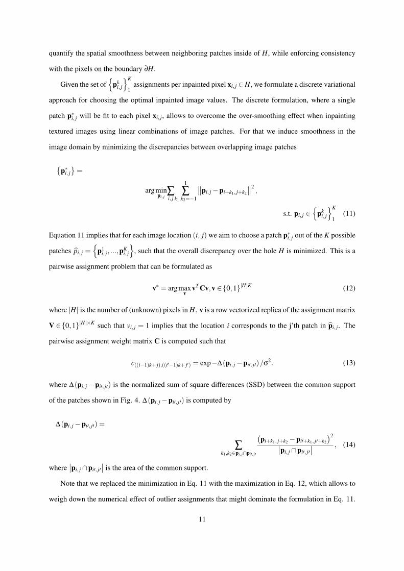
where ∆(pi, j −pi′, j′) is the normalized sum of square differences (SSD) between the common support

of the patches shown in Fig. 4. ∆(pi, j −pi′, j′) is computed by

∆(pi, j −pi′, j′) =

∑k1,k2∈pi, j∩pi′, j′

(pi+k1, j+k2 −pi′+k1, j′+k2

)2∣∣pi, j ∩pi′, j′∣∣ , (14)

where∣∣pi, j ∩pi′, j′

∣∣ is the area of the common support.

Note that we replaced the minimization in Eq. 11 with the maximization in Eq. 12, which allows to

weigh down the numerical effect of outlier assignments that might dominate the formulation in Eq. 11.

11

Figure 4: The normalzed discrepancy between the overlapping patches pi, j and pi′, j′. We compute

the sum of square differences (SSD) over the common support pi, j ∩ pi′, j′, and normalize by its area∣∣pi, j ∩pi′, j′∣∣.

Given the solution of Eq. 12, we paste the chosen candidates at the corresponding missing pixels in H.

As patches overlap, the overlapping pixels are blending by averaging.

Optimizing Eq. 12 is denoted as the Quadratic Assignment Problem (QAP) that is known to be

NP-hard. Hence, the exact inference of the assignments is intractable and we resort to a suboptimal

solution based on spectral relaxation, where we relax the discrete optimization problem in Eq. 12, to an

optimization problem with respect to a continuous variable w

w∗ = argmaxw

wT AwwT w

, w ∈ R|H|k. (15)

This relaxation was used in various computer vision fields [24, 25, 26, 27], and a probabilistic interpre-

tation was first proposed by Zass and Shashua [28] and then extended by Chertok and Keller [29].

The r.h.s. of Eq. 15 is a Rayleigh quotient, and thus, w∗ can be computed as the eigenvector

corresponding to the leading eigenvalue of A. The binary assignment vector v∗ is computed by applying

a discretization procedure to w∗ maximizing the sum of the chosen entries in the vector w∗. This was

shown in [29] to correspond to the maximum likelihood inference of the assignments, under an implicit

probabilistic model. As there are no assignment constraints, we apply a greedy discretization scheme,

where the relaxed assignment vector w ∈ R|H|k is reshaped as an assignment matrix W ∈ R|H|×k. Thus,

each row of W corresponds to the assignments of the set of patches pi, j to a particular pixel xi, j ∈ H,

and we choose the assignment corresponding to the maximal entry in the corresponding row of W.

3.2 Multiscale formulation

We extend the proposed scheme by deriving a multiscale inpainting scheme, using a Gaussian pyramid

of images I0, I1, ..., Im. The inpainting is applied at the coarsest scale Im, and the recovered patches hm are

12

used as anchors in the inpainting of Im−1. The patches in Im−1 whose centers correspond to the locations

of hm are added to the set ∂Hm−1, that is the set of embedding constraints in scale m−1. This approach

is depicted in Fig. 5, where the lower resolution scale is shown in Fig. 5a, while the embedding at the

higher scale (Fig. 5b) utilizes the grid-like anchor embedding points computed in the lower resolution

scale.

(a) (b)

Figure 5: Diffusion embedding at multiple image resolution scales. (a) Embedding eigenvector of lower

scale image. (b) The embedding eigenvectors of a high resolution image replica.

3.3 Affinity measures

In order to achieve a suitable Diffusion embedding as discussed in Section 2.2, one has to choose an

appropriate affinity measure to define the Diffusion kernel in Eq. 2. The chosen metric reflects the sort

of similarity we are interested in, and the resulting image manifold. For instance, using color descriptors

will result in an embedding parameterizing the color manifold of the image. In contrast, in image

inpainting we found it most useful to use texture descriptors.

This reflects the relationship between the Diffusion embedding, the heat kernel and the correspond-

ing PDEs. Implying that previous works based on the variational (and PDE-based) formulations, were

implicitly operating on an image manifold related to its intensity values. Indeed, such schemes [1]

might fail when inpainting textured image regions, and more elaborate schemes that explicitly combine

structure and texture inpainting [11] were derived.

We used two texture descriptors: the first being the Local Binary Pattern (LBP) descriptor [23]

that characterizes the image texture in the vicinity of each pixel. We use this descriptor to define the

13

(a) Source image. (b) LBP-based leading

eigenvector ψ1.

(c) LBP-based ψ1

inpainted by isotropic

PDE.

(d) LBP-based inpainted

image.

(e) ψ1 based on the tex-

ture descriptor of [7].

(f) ψ1 based on [7]

inpainted by the

Best-exemplar.

(g) Best-exemplar based

result.

Figure 6: Comparing the embedding produced by the LBP and Wexler et al.’s [7] texture descriptor.

The LBP produces a smoother embedding that can be inpainted using an isotropic PDE, while Wexler’s

descriptor requires the use of the Best-exemplar [6] for embedding.

similarities between patches in the image. The use of LBP results in a spatially smooth eigenvectors

corresponding to the spatial similarity of the image texture. We also used the texture descriptor pro-

posed by Wexler et al. [7], consisting of (R,G,B, Ix, Iy), being the color channels and the image intensity

gradients. This affinity measure results in a less smooth embedding than the one based on LBP, yet it is

smoother than the source image.

We compare the embedding and inpainting results of the two descriptors in Figs. 6b and 6e. The

embedding produced by the LBP is smoother than that of Wexler’s feature, and while ψ1 in Fig. 6b can

be inpainted using isotropic PDE, the eigenvector in 6e is not as smooth, and we applied the Exemplar-

based approach [6]. Figures 6d and 6g show the comparable inpainting results.

Our approach is summarized in Algorithm 1.

14

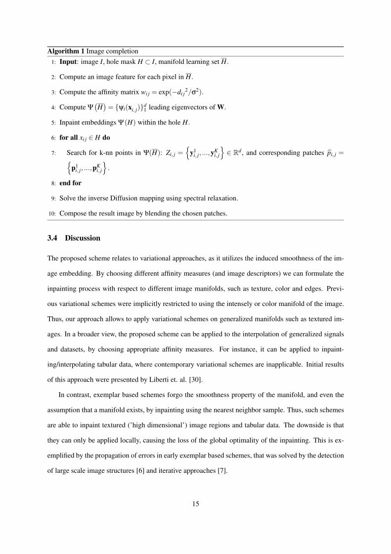
Algorithm 1 Image completion1: Input: image I, hole mask H ⊂ I, manifold learning set H.

2: Compute an image feature for each pixel in H.

3: Compute the affinity matrix wi j = exp(−di j2/σ2).

4: Compute Ψ(H)= ψi(xi, j)d

1 leading eigenvectors of W.

5: Inpaint embeddings Ψ(H) within the hole H.

6: for all xi j ∈ H do

7: Search for k-nn points in Ψ(H): Zi, j =

y1i, j, ...,yK

i, j

∈ Rd , and corresponding patches pi, j =

p1i, j, ...,pK

i, j

.

8: end for

9: Solve the inverse Diffusion mapping using spectral relaxation.

10: Compose the result image by blending the chosen patches.

3.4 Discussion

The proposed scheme relates to variational approaches, as it utilizes the induced smoothness of the im-

age embedding. By choosing different affinity measures (and image descriptors) we can formulate the

inpainting process with respect to different image manifolds, such as texture, color and edges. Previ-

ous variational schemes were implicitly restricted to using the intensely or color manifold of the image.

Thus, our approach allows to apply variational schemes on generalized manifolds such as textured im-

ages. In a broader view, the proposed scheme can be applied to the interpolation of generalized signals

and datasets, by choosing appropriate affinity measures. For instance, it can be applied to inpaint-

ing/interpolating tabular data, where contemporary variational schemes are inapplicable. Initial results

of this approach were presented by Liberti et. al. [30].

In contrast, exemplar based schemes forgo the smoothness property of the manifold, and even the

assumption that a manifold exists, by inpainting using the nearest neighbor sample. Thus, such schemes

are able to inpaint textured (’high dimensional’) image regions and tabular data. The downside is that

they can only be applied locally, causing the loss of the global optimality of the inpainting. This is ex-

emplified by the propagation of errors in early exemplar based schemes, that was solved by the detection

of large scale image structures [6] and iterative approaches [7].

15

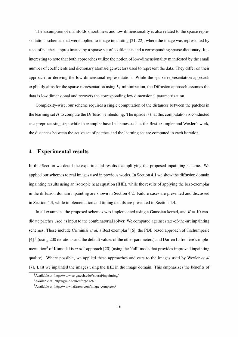
The assumption of manifolds smoothness and low dimensionality is also related to the sparse repre-

sentations schemes that were applied to image inpainting [21, 22], where the image was represented by

a set of patches, approximated by a sparse set of coefficients and a corresponding sparse dictionary. It is

interesting to note that both approaches utilize the notion of low-dimensionality manifested by the small

number of coefficients and dictionary atoms/eigenvectors used to represent the data. They differ on their

approach for deriving the low dimensional representation. While the sparse representation approach

explicitly aims for the sparse representation using L1 minimization, the Diffusion approach assumes the

data is low dimensional and recovers the corresponding low dimensional parametrization.

Complexity-wise, our scheme requires a single computation of the distances between the patches in

the learning set H to compute the Diffusion embedding. The upside is that this computation is conducted

as a preprocessing step, while in exampler based schemes such as the Best-exampler and Wexler’s work,

the distances between the active set of patches and the learning set are computed in each iteration.

4 Experimental results

In this Section we detail the experimental results exemplifying the proposed inpainting scheme. We

applied our schemes to real images used in previous works. In Section 4.1 we show the diffusion domain

inpainting results using an isotropic heat equation (IHE), while the results of applying the best-exemplar

in the diffusion domain inpainting are shown in Section 4.2. Failure cases are presented and discussed

in Section 4.3, while implementation and timing details are presented in Section 4.4.

In all examples, the proposed schemes was implemented using a Gaussian kernel, and K = 10 can-

didate patches used as input to the combinatorial solver. We compared against state-of-the-art inpainting

schemes. These include Criminisi et al.’s Best exemplar1 [6], the PDE based approach of Tschumperle

[4] 2 (using 200 iterations and the default values of the other parameters) and Darren Lafreniere’s imple-

mentation3 of Komodakis et al.’ approach [20] (using the ‘full’ mode that provides improved inpainting

quality). Where possible, we applied these approaches and ours to the images used by Wexler et al

[7]. Last we inpainted the images using the IHE in the image domain. This emphasizes the benefits of

1Available at: http://www.cc.gatech.edu/˜sooraj/inpainting/2Available at: http://gmic.sourceforge.net/3Available at: http://www.lafarren.com/image-completer/

16

operating in the Diffusion domain, that is the focal point of our work.

We are unaware of an objective quality metric for quantifying image inpainting results. Hence, the

inpainting quality assessments made in this section are in essence subjective, but we did our best to be

as impartial as possible.

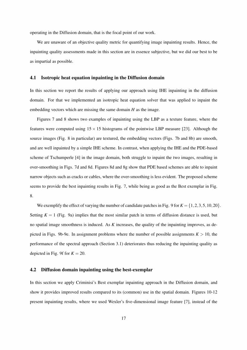
4.1 Isotropic heat equation inpainting in the Diffusion domain

In this section we report the results of applying our approach using IHE inpainting in the diffusion

domain. For that we implemented an isotropic heat equation solver that was applied to inpaint the

embedding vectors which are missing the same domain H as the image.

Figures 7 and 8 shows two examples of inpainting using the LBP as a texture feature, where the

features were computed using 15× 15 histograms of the pointwise LBP measure [23]. Although the

source images (Fig. 8 in particular) are textured, the embedding vectors (Figs. 7b and 8b) are smooth,

and are well inpainted by a simple IHE scheme. In contrast, when applying the IHE and the PDE-based

scheme of Tschumperle [4] in the image domain, both struggle to inpaint the two images, resulting in

over-smoothing in Figs. 7d and 8d. Figures 8d and 8g show that PDE based schemes are able to inpaint

narrow objects such as cracks or cables, where the over-smoothing is less evident. The proposed scheme

seems to provide the best inpainting results in Fig. 7, while being as good as the Best exemplar in Fig.

8.

We exemplify the effect of varying the number of candidate patches in Fig. 9 for K = 1,2,3,5,10,20.

Setting K = 1 (Fig. 9a) implies that the most similar patch in terms of diffusion distance is used, but

no spatial image smoothness is induced. As K increases, the quality of the inpainting improves, as de-

picted in Figs. 9b-9e. In assignment problems where the number of possible assignments K > 10, the

performance of the spectral approach (Section 3.1) deteriorates thus reducing the inpainting quality as

depicted in Fig. 9f for K = 20.

4.2 Diffusion domain inpainting using the best-exemplar

In this section we apply Criminisi’s Best exemplar inpainting approach in the Diffusion domain, and

show it provides improved results compared to its (common) use in the spatial domain. Figures 10-12

present inpainting results, where we used Wexler’s five-dimensional image feature [7], instead of the

17

(a) Original (b) The leading eigenvectors and their

inpaintings

(c) Proposed scheme

(d) Tschumperle et. al. [17] (e) Best exemplar [6] (f) Komodakis et al. [20]

(g) Isotropic heat equation

Figure 7: The inpainting results of the Rice image. The embedding was computed using the LBP texture

descriptor. The upper row in (b) shows the leading embedding eigenvectors with the unknown part H.

The lower row shows the inpainted eigenvectors.

LBP, and the best-exemplar rather than the IHE to inpaint the eigenvectors. In Fig. 10 the proposed

scheme proved superior to the other approaches, while in Figs. 11 and 12 our results are on par with

those of the Best exemplar and Komodakis et al. . These examples emphasize the attributes of the

different schemes. In Fig. 10 the unknown region has a global structure that is best inpainted by a

globally optimal scheme such as ours. In contrast, the missing region in Figs. 11 and 12 is made of

isotropic texture that does not require global optimization, and is thus well inpainted by all schemes.

The embedding smoothness is particularly evident in Fig. 12.

In Fig. 13 we show another example of an image combining texture with global structures, that

are the dark lines. As in Fig. 10, The proposed schemes provides the best inpainting results as it is

able to combine texture synthesis with global optimization. In Fig. 13b we show the three leading

embedding eigenvectors, that are the first three Diffusion coordinates of each pixel. It follows, that

18

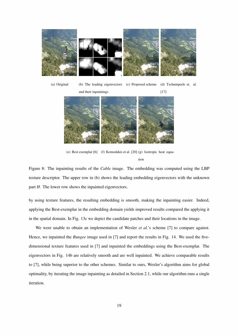
(a) Original (b) The leading eigenvectors

and their inpaintings

(c) Proposed scheme (d) Tschumperle et. al.

[17]

(e) Best exemplar [6] (f) Komodakis et al. [20] (g) Isotropic heat equa-

tion

Figure 8: The inpainting results of the Cable image. The embedding was computed using the LBP

texture descriptor. The upper row in (b) shows the leading embedding eigenvectors with the unknown

part H. The lower row shows the inpainted eigenvectors.

by using texture features, the resulting embedding is smooth, making the inpainting easier. Indeed,

applying the Best-exemplar in the embedding domain yields improved results compared the applying it

in the spatial domain. In Fig. 13c we depict the candidate patches and their locations in the image.

We were unable to obtain an implementation of Wexler et al.’s scheme [7] to compare against.

Hence, we inpainted the Bungee image used in [7] and report the results in Fig. 14. We used the five-

dimensional texture features used in [7] and inpainted the embeddings using the Best-exemplar. The

eigenvectors in Fig. 14b are relatively smooth and are well inpainted. We achieve comparable results

to [7], while being superior to the other schemes. Similar to ours, Wexler’s algorithm aims for global

optimality, by iterating the image inpainting as detailed in Section 2.1, while our algorithm runs a single

iteration.

19

(a) k=1 (b) K = 2 (c) K = 3 (d) K = 5

(e) K = 10 (f) K = 20

Figure 9: Inpainting result of the proposed scheme with respect to different of K nearest neighbors in

the assignment problem (Section 3.1).

4.3 Failure cases

The scheme we propose might fail under certain conditions. We present two such examples in Fig. 15.

The first is the Perrot image in Figs. 15a-15d. The failure is due to the widening of the unknown regions

H in the upper row of Fig. 15. The widening occurs due to the use of 15×15 image patches to define the

LBP descriptors. Thus, in order to compute the LBP descriptor on the boundary ∂H, we had to widen

H by 30 pixels overall. In contrast, PDE-based schemes use a two-pixels wide boundary ∂H, but might

fail to inpaint textured areas. This is depicted in Fig. 15d, where we applied the PDE-based approach of

Tschumperle et. al. [17]. Although the inpainting has no artifacts, close visual inspection reveals that

the inpainted parts are over-smoothed and that texture details are lost. The second example is shown in

Figs. 15d-15f, where the LBP descriptors fail to correctly characterize the image texture. This is evident

in the embedding of the first eigenvector in Figs. 15e.

20

(a) Original (b) The leading embedding eigenvectors and

their inpaintings.

(c) Proposed scheme

(d) Tschumperle et. al. [17] (e) Best exemplar [6] (f) Komodakis et al. [20] (g) Isotropic heat equation

Figure 10: Image completion using the five-dimensional texture descriptor of [7] and best-exemplar

inpainting of the eigenvectors.

(a) Original (b) The leading embedding

eigenvectors and their inpaint-

ings.

(c) Proposed scheme (d) Tschumperle et. al. [17]

(e) Best exemplar [6] (f) Komodakis et al. [20] (g) Isotropic heat equation

Figure 11: Image completion using the five-dimensional texture descriptor of [7] and best-exemplar

inpainting of the eigenvectors.

21

(a) Original (b) Eigenvectors ψ1 ÷ψ3 and

their inpaintings.

(c) Eigenvectors ψ10 ÷ ψ12

and their inpaintings.

(d) Proposed scheme

(e) Tschumperle et. al. [17] (f) Best exemplar [6] (g) Komodakis et al. [20] (h) Isotropic heat equation

Figure 12: Image completion using the five-dimensional texture descriptor of [7] and best-exemplar

inpainting of the eigenvectors. In (b) and (c) we show some of the embedding eigenvectors. By using

the five-dimensional texture descriptor we obtain a smooth embedding.

4.4 Implementation issues

The proposed scheme was implemented in Matlab and the timing was measured on a Quad4-based com-

puter running at 2.6GHz. When inpainting a 200× 200 image, the computation of the sparse distance

matrix between the LBP features, used to compute the embedding required 11 minutes. Applying the

IHE on the Diffusion embedding vectors took a minute, while running the Best-exampler inpainting

required three minutes. The approximate inverse mapping using the spectral relaxation lasted three min-

utes on average. Thus, the overall inpainting takes 15 and 17 minutes, for the IHE and Best Exampler-

based schemes, respectively. This timing can be significantly shortened by improving the computation

of the patch distance matrix using the Patchmatch approach [16] and its variations.

5 Conclusions

In this work we a proposed a Diffusion based framework for image completion. The crux of our approach

is to utilize the Diffusion embedding to induce application specific smoothness over the inpainted im-

age. The induced smoothness is manifested by the smoothness of the embedding eigenvectors, when

22

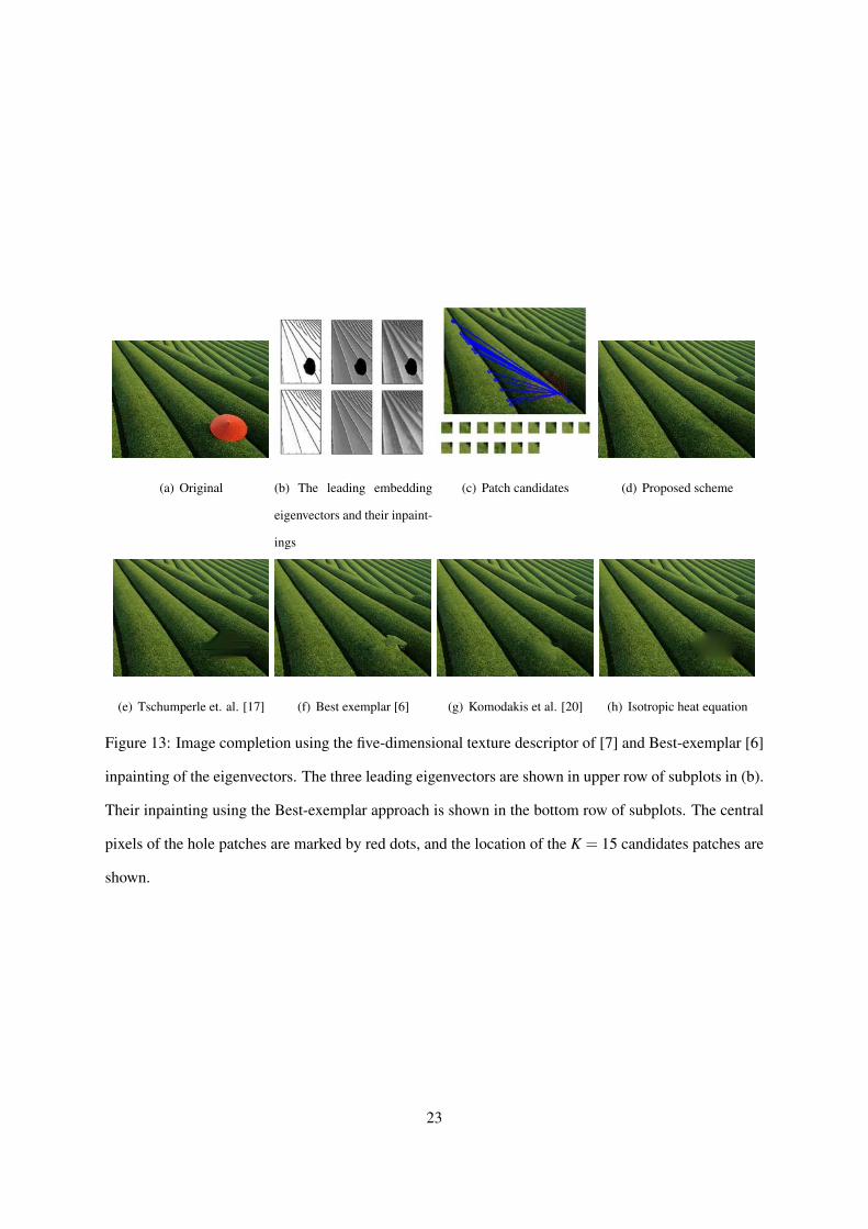
(a) Original (b) The leading embedding

eigenvectors and their inpaint-

ings

(c) Patch candidates (d) Proposed scheme

(e) Tschumperle et. al. [17] (f) Best exemplar [6] (g) Komodakis et al. [20] (h) Isotropic heat equation

Figure 13: Image completion using the five-dimensional texture descriptor of [7] and Best-exemplar [6]

inpainting of the eigenvectors. The three leading eigenvectors are shown in upper row of subplots in (b).

Their inpainting using the Best-exemplar approach is shown in the bottom row of subplots. The central

pixels of the hole patches are marked by red dots, and the location of the K = 15 candidates patches are

shown.

23

(a) source image (b) The leading embed-

ding eigenvectors and

their inpaintings.

(c) Proposed scheme (d) Best exemplar result

[6]

(e) Wexler et al. result

[7]

(f) Tschumperle et. al.

[17]

(g) Komodakis et al.

[20]

Figure 14: Inpainting results of the Bungee image. The image in (b) was inpainted using a five-

dimensional texture feature [7], and Criminisi’s Best exemplar inpainting of the embedding vectors.

24

(a) Parrot image (b) The leading embedding eigenvectors

and their inpaintings.

(c) Inpainting results by

the proposed scheme

(d) Tschumperle et. al.

[17]

(e) Building image (f) The leading embedding

eigenvectors and their inpaint-

ings.

(g) Inpainting re-

sults by the pro-

posed scheme.

Figure 15: Failure cases.In (d) we show the inpainting by Tschumperle et. al. [17].

25

computed using appropriate affinity measures, such as the LBP texture features. Thus, we can apply

PDE-based inpainting schemes that are commonly only applicable to smooth images, to textured im-

ages. In particular, such schemes allow to achieve global inpainting optimality and can be applied to

inpainting large-scale holes. We also showed that the use of the Best-exemplar in the diffusion domain,

rather than in image intensity domain, yields improved inpainting results. In order to compute an ap-

proximate inverse-diffusion mapping, we introduce a novel approach based on discrete optimization,

with a corresponding spectral relaxation. The proposed inpainting scheme compares favorably with

previous state-of-the-art methods. A major upside of the proposed scheme, is that it can be applied to

general datasets such as tabular data, and we reserve that for future work.

References

[1] M. Bertalmio, G. Sapiro, V. Caselles, and C. Ballester, “Image inpainting,” in Proceedings of the

27th annual conference on Computer graphics and interactive techniques, SIGGRAPH ’00, (New

York, NY, USA), pp. 417–424, ACM Press/Addison-Wesley Publishing Co., 2000.

[2] M. Bertalmıo, “Strong-continuation, contrast-invariant inpainting with a third-order optimal PDE,”

IEEE Transactions on Image Processing, vol. 15, no. 7, pp. 1934–1938, 2006.

[3] J. Shen, S. H. Kang, and T. F. Chan, “Euler’s elastica and curvature-based inpainting,” SIAM Jour-

nal of Applied Mathematics, vol. 63, no. 2, pp. 564–592, 2003.

[4] D. Tschumperle, “Fast anisotropic smoothing of multi-valued images using curvature-preserving

pde’s,” International Journal of Computer Vision, vol. 68, no. 1, pp. 65–82, 2006.

[5] A. A. Efros and T. K. Leung, “Texture synthesis by non-parametric sampling,” in ICCV, pp. 1033–

1038, 1999.

[6] A. Criminisi, P. Prez, and K. Toyama, “Region filling and object removal by exemplar-based image

inpainting,” IEEE Transactions on Image Processing, vol. 13, pp. 1200–1212, 2004.

[7] Y. Wexler, E. Shechtman, and M. Irani, “Space-time completion of video,” Pattern Analysis and

Machine Intelligence, IEEE Transactions on, vol. 29, pp. 463 –476, march 2007.

26

[8] I. Drori, D. Cohen-Or, and H. Yeshurun, “Fragment-based image completion,” ACM Trans. Graph.,

vol. 22, pp. 303–312, July 2003.

[9] J. Hays and A. A. Efros, “Scene completion using millions of photographs,” ACM Trans. Graph.,

vol. 26, July 2007.

[10] J. Mairal, M. Elad, and G. Sapiro, “Sparse representation for color image restoration,” IEEE Trans-

actions on Image Processing, vol. 17, no. 1, pp. 53–69, 2008.

[11] A. Bugeau, M. Bertalmıo, V. Caselles, and G. Sapiro, “A comprehensive framework for image

inpainting,” Image Processing, IEEE Transactions on, vol. 19, pp. 2634 –2645, oct. 2010.

[12] M. Bertalmıo, L. A. Vese, G. Sapiro, and S. Osher, “Simultaneous structure and texture image

inpainting,” in CVPR (2), pp. 707–712, 2003.

[13] R. Coifman and S. Lafon, “Diffusion maps,” Applied and Computational Harmonic Analysis: Spe-

cial issue on Diffusion Maps and Wavelets, vol. 22, pp. 5–30, July 2006.

[14] M. Belkin and P. Niyogi, “Laplacian eigenmaps for dimensionality reduction and data representa-

tion,” Neural Computation, vol. 6, pp. 1373–1396, June 2003.

[15] M. Leordeanu and M. Hebert, “A spectral technique for correspondence problems using pairwise

constraints,” in International Conference of Computer Vision (ICCV), vol. 2, pp. 1482 – 1489,

October 2005.

[16] C. Barnes, E. Shechtman, A. Finkelstein, and D. B. Goldman, “Patchmatch: a randomized corre-

spondence algorithm for structural image editing,” ACM Trans. Graph., vol. 28, pp. 24:1–24:11,

July 2009.

[17] D. Tschumperle and R. Deriche, “Vector-valued image regularization with pdes: a common frame-

work for different applications,” Pattern Analysis and Machine Intelligence, IEEE Transactions

on, vol. 27, pp. 506 –517, april 2005.

[18] S. Masnou and J.-M. Morel, “Level lines based disocclusion,” in ICIP (3), pp. 259–263, 1998.

[19] O. Le Meur, J. Gautier, and C. Guillemot, “Examplar-based inpainting based on local geometry,”

in ICIP, (Brussel, Belgique), 2011.

27

[20] N. Komodakis and G. Tziritas, “Image completion using efficient belief propagation via priority

scheduling and dynamic pruning,” Image Processing, IEEE Transactions on, vol. 16, pp. 2649

–2661, nov. 2007.

[21] J. Mairal, M. Elad, and G. Sapiro, “Sparse representation for color image restoration,” Image

Processing, IEEE Transactions on, vol. 17, pp. 53 –69, jan. 2008.

[22] M. Elad, J.-L. Starck, P. Querre, and D. Donoho, “Simultaneous cartoon and texture image in-

painting using morphological component analysis (mca),” Applied and Computational Harmonic

Analysis, vol. 19, no. 3, pp. 340 – 358, 2005. Computational Harmonic Analysis - Part 1.

[23] T. Ojala, M. Pietikainen, and T. Maenpaa, “Multiresolution gray-scale and rotation invariant texture

classification with local binary patterns,” IEEE Trans. Pattern Anal. Mach. Intell., vol. 24, no. 7,

pp. 971–987, 2002.

[24] J. Shi and J. Malik, “Normalized cuts and image segmentation,” Pattern Analysis and Machine

Intelligence, IEEE Transactions on, vol. 22, no. 8, pp. 888–905, 2000.

[25] M. Leordeanu and M. Hebert, “A spectral technique for correspondence problems using pairwise

constraints,” in ICCV, vol. 2, pp. 1482 – 1489, 2005.

[26] A. Egozi, Y. Keller, and H. Guterman, “Improving shape retrieval by spectral matching and meta

similarity,” Image Processing, IEEE Transactions on, vol. 19, pp. 1319 –1327, may 2010.

[27] M. Chertok and Y. Keller, “Spectral symmetry analysis,” IEEE Transactions on Pattern Analysis

and Machine Intelligence, vol. 32, no. 7, pp. 1227–1238, 2010.

[28] R. Zass and A. Shashua, “Probabilistic graph and hypergraph matching,” in Computer Vision and

Pattern Recognition, 2008. CVPR 2008. IEEE Conference on, pp. 1–8, June 2008.

[29] M. Chertok and Y. Keller, “Efficient high order matching,” IEEE Transactions on Pattern Analysis

and Machine Intelligence, vol. 32, pp. 2205–2215, 2010.

[30] E. Liberty, M. Almagor, S. Zucker, Y. Keller, and R. Coifman, “Scoring psychological question-

naires using geometric harmonics,” in Snowbird Learning workshop, 2007.

28