inﬂuence of multi-step topography on barotropic waves and...

Ocean Modelling 14 (2006) 45–60

www.elsevier.com/locate/ocemod

Influence of multi-step topography on barotropic wavesand consequences for numerical modeling

Dmitry S. Dukhovskoy *, Steven L. Morey, James J. O’Brien

Florida State University, Center for Ocean-Atmospheric Prediction Studies, Tallahassee, FL 32306-2840, USA

Received 8 August 2005; received in revised form 28 February 2006; accepted 2 March 2006Available online 18 April 2006

Abstract

Propagation of barotropic topographic Rossby waves (TRWs) and Kelvin type waves over topography consisting ofmultiple steps is investigated. The transformation of the wave solution from one limiting case with narrow and small stepsmost closely approximating a continuous slope to another limiting case with wide and high steps is analyzed. The analysisis based on the numerical simulation of the topographic waves by employing a model with r-level (terrain following)vertical coordinates and several Z-level (geopotential following) vertical coordinate model configurations with a varyingnumber of vertical levels. An analytical solution for frequencies of quasi-geostrophic waves over a multi-step topographyis derived to examine how the wave solution transforms for different vertical resolution (yielding different step sizes).Analysis of the model and analytical results suggests criteria for the vertical resolution of a Z-level model with a giventopography to support TRW-like solutions and to prevent the formation of artificial edge-trapped waves. When the modelhas a coarse vertical resolution yielding wide steps compared to the trapping scale of the wave the quasi-geostrophic wavesconvert to double Kelvin waves trapped along the step edges. In the model with fine vertical resolution there is a transitionfrom the quasi-geostrophic wave to the TRW solution.� 2006 Elsevier Ltd. All rights reserved.

Keywords: Numerical models; Ocean mathematical models; Topographic waves; Double Kelvin waves; Continental shelves; Shelf waves

1. Introduction

Topographic Rossby waves (TRWs) are crucial to the numerical simulation of large-scale ocean dynamicsbecause they propagate energy over long distances and are important means of adjustment along the bound-aries (Gerdes, 1993). The ability of a numerical ocean model to realistically simulate TRWs is largelyinfluenced by the accuracy of the approximation of the topography, particularly in regions with slopes, inthe model. Misrepresentation of the bottom slopes in a model can lead to an inaccurate simulation oftopographic waves with a modified dispersion relation. For a given spatial resolution, the representation

1463-5003/$ - see front matter � 2006 Elsevier Ltd. All rights reserved.

doi:10.1016/j.ocemod.2006.03.002

* Corresponding author. Tel.: +1 850 644 1168; fax: +1 850 644 4841.E-mail addresses: [email protected] (D.S. Dukhovskoy), [email protected] (S.L. Morey), [email protected]

(J.J. O’Brien).

mailto:[email protected]



46 D.S. Dukhovskoy et al. / Ocean Modelling 14 (2006) 45–60

of topography varies in models depending on the way of discretizing the vertical coordinate. There are threemain strategies for discretization of the vertical coordinate in models: r- or terrain-following coordinates(Blumberg and Mellor, 1987); isopycnal coordinates (Bleck, 1998); and Z-level or geopotential coordinates(Bryan, 1969).

Z-level models approximate a slope as several steps in which the width and height depend on the verticaland horizontal resolution of the model. There has been wide discussion in the literature on the ‘‘weakness’’ ofZ-level models stemming from their step-wise representation of the bottom topography (Killworth et al., 1991;Gerdes, 1993; Martin et al., 1998; Pacanowski and Gnanadesikan, 1998). For example, Pacanowski andGnanadesikan (1998) have shown that Z-level models have problems realistically resolving the bottom topog-raphy when slopes are less than the grid cell aspect ratio (dz/dx) leading to an inaccurate dispersion relationfor topographic waves. Despite the problems with bottom representation, Z-level models have the advantagesof accurate calculation of the horizontal pressure gradient and a possibly smaller error in diapycnal diffusion(Gerdes, 1993). Several approaches for solving the problem of topography representation in Z-level modelshave been recently discussed in the literature: ‘‘shaved cell’’ technology (Adcroft et al., 1997); a partial cellapproach (Pacanowski and Gnanadesikan, 1998); a hybrid model with a sigma surface at the bottom level(Gerdes, 1993; Beckmann and Doscher, 1997; Marshall et al., 1997); and an embedded bottom boundary layerscheme (Song and Chao, 2000).

Z-level models are widely used for numerical ocean simulation (Zhang et al., 1999; Nakano and Sugino-hara, 2002; Steiner et al., 2004; Kara et al., 2005), especially in the Global Climate models (GCMs) (Gentet al., 1998; Holland et al., 1998; Saunders et al., 1999; Flato et al., 2000; Roberts et al., 2003; Zhang andRothrock, 2003). The poor representation of topography in Z-level models casts doubt on the ability of thisclass of models to simulate topographic waves. In Z-level models with coarse vertical discretization, the gentleslope is represented by several wide and high steps which, due to potential vorticity conservation, may preventwater parcels from crossing isobaths. Thus, TRWs may not be supported in this type of model. This problemcan be viewed from a different angle, namely, can a TRW exist over a bottom with a multi-step topography?An anticipated answer to this question is ‘‘yes’’ if the steps are sufficiently small to provide a good approxi-mation of the gently sloping bottom. So the question becomes: how small is ‘‘sufficiently small’’, and whathappens to the TRW if the steps are not ‘‘sufficiently small’’?

This paper seeks to answer the question of how large the steps can be so that TRWs can still exist. At thesame time the posed question can be considered as an attempt to estimate the criteria for the Z-level verticalresolution that allows a numerical model to adequately simulate TRWs for a given slope. The study is carriedout by conducting model experiments with r-level and Z-level vertical coordinate systems with different ver-tical resolutions. The effect of different vertical resolutions in Z-level models, and thus step size, on simulationsof TRWs is discussed with particular emphasis on the dispersion relations of the waves. An analytical model ofa topographic wave along multi-step topography in a barotropic uniformly rotating ocean is developed whichreproduces the transformation of the wave solution as the step size (width and height) changes similar to thenumerical model.

2. Fundamentals of barotropic topographic Rossby waves

Topographic Rossby waves play an important role in the ocean dynamics in regions where the slope of thebottom topography is sufficiently large so as to dominate the planetary b-effect. From the theory of planetarywaves (e.g., Pedlosky, 1987), when a water parcel is displaced from its state of rest such that it crosses isolinesof ambient potential vorticity the water parcel reacts by changing its relative vorticity. New fluid parcelsentrained by the swirling motions move meridionally acquiring either positive (when moving toward regionsof lower ambient potential vorticity) or negative (toward higher potential vorticity values) relative vorticity.This results in the westward propagation of the wave pattern. In the presence of a gently varying ocean bottomwhen the b-effect can be neglected, the topographic parameter starts playing the role of the planetary number(bLf�1, where b is the beta parameter, L is meridional length scale, and f is the Coriolis parameter). Bottomtopography controls the dynamics of long waves (frequency, phase and group speed) in a uniformly rotatingbarotropic ocean. TRWs differ from planetary Rossby waves in that the magnitude of relative vorticity mustchange proportionally with the water column depth.

D.S. Dukhovskoy et al. / Ocean Modelling 14 (2006) 45–60 47

The condition when topography dominates the b-effect is (LeBlond and Mysak, 1977)

jH y j > HR�10 ; ð1Þ

where

R0 ¼ f0b ¼ R tan u0; ð2Þ
R is the Earth radius and u0 is latitude. Evidence of the existence of topographically dominated waves hasbeen found in different parts of the world ocean (Rhines, 1969; Thompson, 1971). A detailed analysis ofthe northern Gulf of Mexico seafloor in Lugo-Fernandez and Morin (2004), for instance, reveals the existenceof slopes that can support TRWs, which are thought to be responsible for the strong deep currents in thatregion (Hamilton and Lugo-Fernandez, 2001).
The importance of vertical density stratification to topographic waves has been discussed in the literature(e.g, Wang and Mooers, 1976). Being characterized by large horizontal scales resulting in a small Burger num-ber (R2

i =L2, where Ri is the internal Rossby radius and L is the horizontal length scale), long TRWs arevirtually unaffected by stratification (LeBlond and Mysak, 1978). It has been shown that for long TRWson a shelf (wavelength longer than a shelf width), the barotropic model qualitatively reproduces the majorfeatures of the vertically stratified ocean (Brooks and Mooers, 1977). Clarke and Brink (1985), through scaleanalysis of the shallow water equations, show that the response of a wide shelf (with small Burger number) tosynoptic wind fluctuations should be barotropic. In particular, Mitchum and Clarke (1986) suggest that largescale motions on the West Florida Shelf can mostly be explained by barotropic dynamics.

The barotropic motions over variable depth are governed by the linearized equations (Pedlosky, 1987)

ut � fvþ ggx ¼ 0; ð3aÞvt þ fuþ ggy ¼ 0; ð3bÞ½ðH þ gÞu�x þ ½ðH þ gÞv�y þ gt ¼ 0. ð3cÞ

Several analytical solutions have been derived for certain offshore bathymetry profiles (H(y)) (e.g., LeBlondand Mysak, 1978). The influence of different types of topography on the topographic waves has been widelydiscussed in the literature (Longuet-Higgins, 1968a,b; Rhines, 1969; Sandstrom, 1969; LeBlond and Mysak,1977, 1978; Cushman-Roisin and O’Brien, 1983; Pickart, 1995). Generally speaking, all the topography relatedstudies of long waves fall into two categories: (1) waves over continuous slopes such as those given by linearfunctions (Cushman-Roisin, 1994), exponential functions (LeBlond and Mysak, 1978), steep continuousslopes approximated with hyperbolic functions (Longuet-Higgins, 1968a), concave upward depth profiles(Ball, 1967) and concave downward depth profiles (Robinson, 1964); (2) waves over abrupt topography thatincludes single step (Longuet-Higgins, 1968b; Larsen, 1969) or different kinds of edges described in detail inRhines (1969). Much less attention, if any, has been paid to multi-step topography. However this type of prob-lem might be of interest to researchers employing numerical ocean models and especially to those who useZ-level models which approximate topography as a number of steps.

3. Design of the model experiments

A long (Lx = 480 km) barotropic shelf in the northern hemisphere with variable depth H on an f-plane isconsidered (Fig. 1). The Coriolis parameter is calculated for latitude 30� N. The width of the shelf (Ly) is100 km. The abscissa is oriented along the coast and the ordinate points offshore. The boundary conditionsat x = 0 and x = Lx are cyclic, and at the y = Ly the boundary is open. The bottom depth has an exponentialprofile in the offshore direction

HðyÞ ¼ H 0 expð2ayÞ; ð4Þ
where H0 is the depth at the coast and 2a determines the cross-shelf e-folding scale of the bathymetry (Table1). For this depth profile, the analytical solution of Eq. (3) under the rigid lid approximation (which is valid forthe studied case, since the long waves of interest satisfy the necessary condition for rigid lid assumptionf 2=gHk2
h � 1, where k�1h is the wave length scale) is (LeBlond and Mysak, 1978; Martin et al., 1998)

Fig. 1. Schematic of the model domain with an exponential depth profile.

Table 1Model parameters

Parameters Values

Shelf length, Lx (km) 480Shelf width, Ly (km) 100e-folding scale of the bathymetry, (2a)�1 (km) 40Cross-shelf wave length, ky (km) 200Along-shelf wave length, kx (km) Lx/n, n = 1, . . . , 6Scaling parameter, A 5000Coriolis parameter, f (s�1) 7.29 · 10�5

Horizontal resolution, Dx, Dy (km) 4


g ¼ Agkx

expð�ayÞ½ðxa� fkxÞ sinðkyyÞ þ xky cosðkyyÞ� cosðkxx� xtÞ; ð5aÞ

u ¼ A expð�ayÞ½a sinðkyyÞ þ ky cosðkyyÞ� cosðkxx� xtÞ; ð5bÞv ¼ Akx expð�ayÞ sinðkyyÞ sinðkxx� xtÞ; ð5cÞ

where kx and ky are the along-shelf and cross-shelf wave numbers, respectively, and x is the frequency. A is ascale parameter which defines the amplitude of the wave. The choice of the scale parameter is made based onthe requirement for the validity of linearization which states that the particle velocity should be smaller thanthe phase speed ðj~uj=j~cj � 1Þ (LeBlond and Mysak, 1978; Pedlosky, 1987). The parameter A is taken to be5000, which gives a maximum amplitude of the sea surface height (SSH) of �0.03 m and maximum velocityof �0.15 m/s.

The simulations are performed with the Navy Coastal Ocean Model (NCOM). The NCOM is a primitiveequation, three-dimensional, thermodynamic, hydrostatic, free surface ocean model with the Arakawa C grid(Martin, 2000). The free surface is treated implicitly. The NCOM uses an orthogonal-curvilinear horizontalgrid, a hybrid r/Z-level vertical grid and various numerical, horizontal mixing, and vertical mixing options.The hybrid vertical grid allows one to include r levels in the upper ocean which guarantees good approxima-tion of topography in shallow regions and Z levels for the deep ocean. The number of vertical levels can be setto acquire the desired vertical resolution. Also the model can be designed as either a pure r-level or Z-levelmodel (with a free surface). The control run is performed with 1r level which, for a given depth profile, mostrealistically resolves the topography. Then, several simulations are run using Z levels with different numbers oflevels providing the desired number of steps varying from 2 to 24 approximating the slope (Fig. 2). Withineach experiment, the width of the steps is kept the same by using logarithmic vertical resolution. No forcingis applied in the model. Sidewall and bottom boundary conditions for momentum are free-slip. For eachexperiment, the model is initialized with the analytical solutions (5) with the cross-shelf wave lengthky = 160 km for six along-shelf wave lengths kx = Lx/n, n = 1, . . . , 6. The model is integrated for 20 daysand output is saved every 6 h of integration.

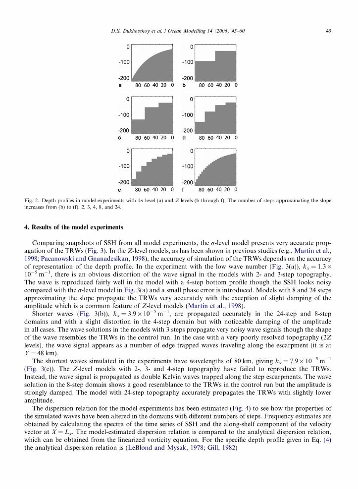
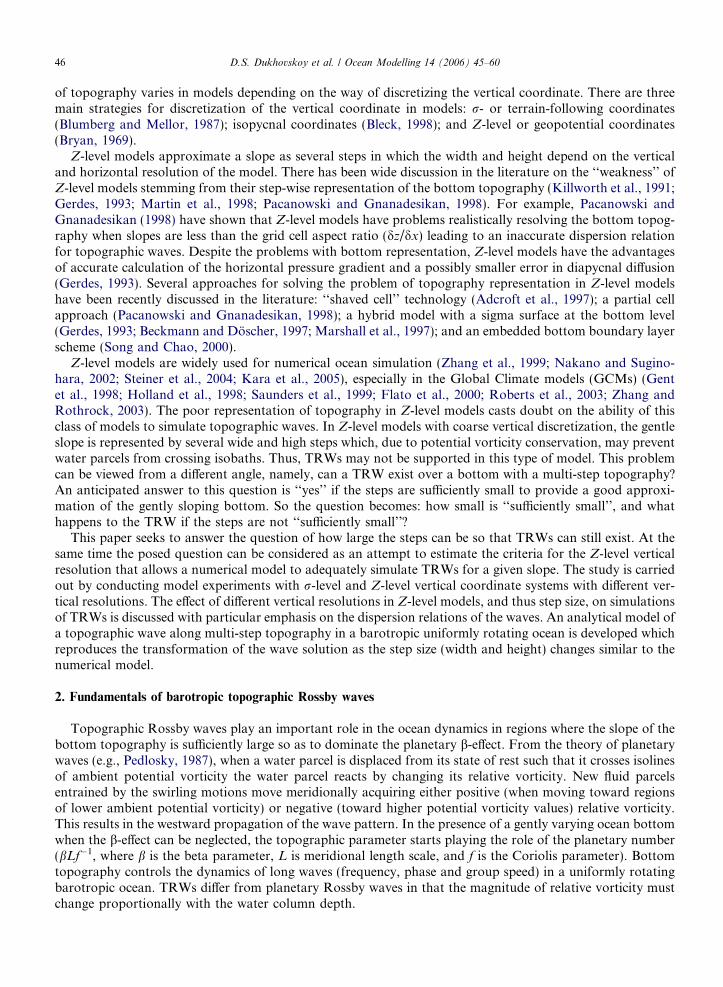
Fig. 2. Depth profiles in model experiments with 1r level (a) and Z levels (b through f). The number of steps approximating the slopeincreases from (b) to (f): 2, 3, 4, 8, and 24.


4. Results of the model experiments

Comparing snapshots of SSH from all model experiments, the r-level model presents very accurate prop-agation of the TRWs (Fig. 3). In the Z-level models, as has been shown in previous studies (e.g., Martin et al.,1998; Pacanowski and Gnanadesikan, 1998), the accuracy of simulation of the TRWs depends on the accuracyof representation of the depth profile. In the experiment with the low wave number (Fig. 3(a)), kx = 1.3 ·10�5 m�1, there is an obvious distortion of the wave signal in the models with 2- and 3-step topography.The wave is reproduced fairly well in the model with a 4-step bottom profile though the SSH looks noisycompared with the r-level model in Fig. 3(a) and a small phase error is introduced. Models with 8 and 24 stepsapproximating the slope propagate the TRWs very accurately with the exception of slight damping of theamplitude which is a common feature of Z-level models (Martin et al., 1998).

Shorter waves (Fig. 3(b)), kx = 3.9 · 10�5 m�1, are propagated accurately in the 24-step and 8-stepdomains and with a slight distortion in the 4-step domain but with noticeable damping of the amplitudein all cases. The wave solutions in the models with 3 steps propagate very noisy wave signals though the shapeof the wave resembles the TRWs in the control run. In the case with a very poorly resolved topography (2Z

levels), the wave signal appears as a number of edge trapped waves traveling along the escarpment (it is atY = 48 km).

The shortest waves simulated in the experiments have wavelengths of 80 km, giving kx = 7.9 · 10�5 m�1

(Fig. 3(c)). The Z-level models with 2-, 3- and 4-step topography have failed to reproduce the TRWs.Instead, the wave signal is propagated as double Kelvin waves trapped along the step escarpments. The wavesolution in the 8-step domain shows a good resemblance to the TRWs in the control run but the amplitude isstrongly damped. The model with 24-step topography accurately propagates the TRWs with slightly loweramplitude.

The dispersion relation for the model experiments has been estimated (Fig. 4) to see how the properties ofthe simulated waves have been altered in the domains with different numbers of steps. Frequency estimates areobtained by calculating the spectra of the time series of SSH and the along-shelf component of the velocityvector at X = Lx. The model-estimated dispersion relation is compared to the analytical dispersion relation,which can be obtained from the linearized vorticity equation. For the specific depth profile given in Eq. (4)the analytical dispersion relation is (LeBlond and Mysak, 1978; Gill, 1982)

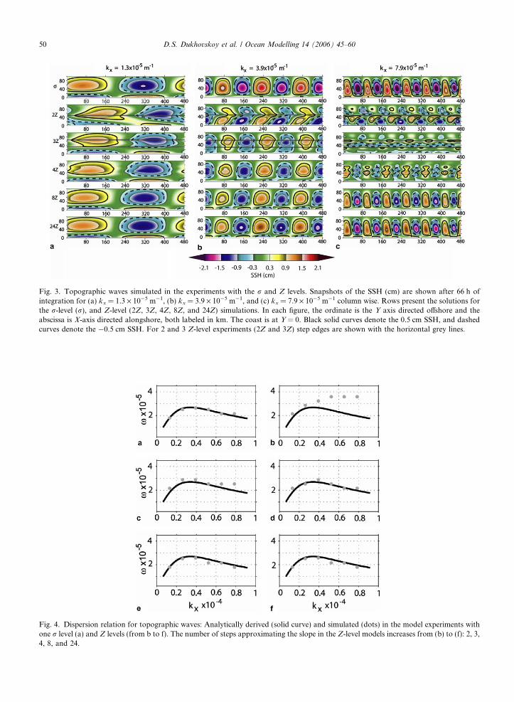
Fig. 4.one r4, 8, a

Fig. 3. Topographic waves simulated in the experiments with the r and Z levels. Snapshots of the SSH (cm) are shown after 66 h ofintegration for (a) kx = 1.3 · 10�5 m�1, (b) kx = 3.9 · 10�5 m�1, and (c) kx = 7.9 · 10�5 m�1 column wise. Rows present the solutions forthe r-level (r), and Z-level (2Z, 3Z, 4Z, 8Z, and 24Z) simulations. In each figure, the ordinate is the Y axis directed offshore and theabscissa is X-axis directed alongshore, both labeled in km. The coast is at Y = 0. Black solid curves denote the 0.5 cm SSH, and dashedcurves denote the �0.5 cm SSH. For 2 and 3 Z-level experiments (2Z and 3Z) step edges are shown with the horizontal grey lines.


Dispersion relation for topographic waves: Analytically derived (solid curve) and simulated (dots) in the model experiments withlevel (a) and Z levels (from b to f). The number of steps approximating the slope in the Z-level models increases from (b) to (f): 2, 3,nd 24.


x ¼ 2akxf

k2x þ k2

y þ a2. ð6Þ

The dispersion relation of the r-level model matches the analytical relation nearly perfectly (Fig. 4a). TheZ-level models with bathymetry well-resolved by 8 and 24 steps (Fig. 4e and f) also demonstrate a very goodagreement with the analytical dispersion relation. The models with 3 and 4 Z levels (Fig. 4c and d) provide anaccurate simulation of the long topographic waves but for the short waves the dispersion relation does notchange with the wave number (last three dots in 4c and last two in 4d). As discussed later, this is a character-istic feature of edge-trapped waves. The model with 2 steps failed to support the TRWs simulated by the con-trol run and the propagating features have a fundamentally different dispersion relation (Fig. 4b).

The important issue in all this is whether the simulated waves propagate energy in the proper direction. Awell-known feature stemming from the dispersion relation of the shelf waves is that long waves transport theenergy in the same direction as their phase speed with the coast on the right in the Northern Hemisphere (i.e.,ox/okx > 0) and short waves transport energy in the opposite direction. In the r-level model and Z-level mod-els with 8- and 24-step topography, the energy is propagated by all simulated waves in the proper direction.Short waves (kx > 0.5 · 10�5 m�1 in Fig. 4b and c and kx > 0.6 · 10�5 m�1 in Fig. 4d) simulated in the Z-levelmodels with poorly resolved topography do not propagate energy at all, evidenced by the frequency becomingindependent of the wave number for short waves. The long wave energy propagation direction agrees with theTRW behavior for all cases.

The analysis of model experiments with different vertical configurations reveals that Z-level models canreproduce wave solutions similar to the r-level model. Changing only the vertical resolution in the Z-levelmodel experiments (keeping all other parameters in the model the same) results in different types of topo-graphic waves with dispersion relation different from that of the TRWs. The question is why the dispersionrelation looks different for Z-level models with poorly resolved topography.

5. Analysis and discussion

An analytical approach is chosen to investigate the problem outlined in the previous section. A dispersionrelation of a topographic wave over a multi-step topography is sought and analyzed for steps of differentwidth and height. It is anticipated that when the steps are small, the dispersion relation of the wave shouldapproach the dispersion relation of the TRWs given by Eq. (6) and shown in Fig. 4. The idea is based onVolterra’s principle (Volterra, 1887, 1959) of passage from finiteness to infinity used in the numerical integra-tion of differential equations. The principle states that the exact solution can be approximated to an infinitelysmall precision by infinitely small steps. This approach is used by Munk et al. (1964) to solve the linearizedwave equation over a sloping bottom, where the sloping bottom is replaced by a series of discontinuous stepsand the differential equations are solved for each constant depth layer integrating into a single wave solution.

5.1. Dispersion relation of a long wave over a multi-step topography

A long free wave of small amplitude over a multi-step topography is considered

ut � fv ¼ �ggx; ð7aÞvt þ fu ¼ �ggy ; ð7bÞgt ¼ �ðHuÞx � ðHvÞy . ð7cÞ

Let the bottom topography be step-like with N steps aligned with the Y-axis pointed to the sea (Fig. 5). Thedepth at step j is hj and the step width is Dj. The Y-axis is split into Ny 0 axis segments for each step(0 < y 0 < Dj), such that Zj(0) designates the amplitude at the beginning of the jth step and Z(Dj) is the ampli-tude at the end of the step. Here, the goal is to seek the solution for the wave amplitude as a function of thecross-shelf direction. The waves are assumed to have a component traveling parallel to shore

ðf; u; vÞ ¼ ðZðyÞ;UðyÞ; V ðyÞÞ exp½iðkxx� xtÞ�. ð8Þ

Fig. 5. A long wave over a multi-step topography.


Following Larsen (1969), from (7) and (8) the wave amplitude, Z, within each step satisfies the equation

d2Zj

dy2� mjZj ¼ 0; ð9Þ

where j is the step number and mj ¼ s2j ¼ k2

x �ðx2�f 2Þ

ghj.

Depending on the value of m, three types of solutions of (9) are possible

Z ¼ c1 expð�syÞ þ c2 expðsyÞ; m > 0 ð10aÞZ ¼ c1 þ c2y; m ¼ 0 ð10bÞZ ¼ c1 cosðsyÞ þ c2 sinðsyÞ; m < 0. ð10cÞ

In this case, the wave frequency is subinertial leading to m > 0. Thus the only solution of interest is (10a) whichcan be rewritten as

Z ¼ a coshðsyÞ þ b sinhðsyÞ; ð11Þ
where a and b are constants and s > 0. Actually in the studied case, k2
x � jðx2 � f 2Þ=ghij and therefore s � jkxj.From Munk et al. (1964), the boundary conditions (BC) at the coastline require that the flow normal to the

shore (h Æ V) must vanish. Also the amplitude at Y = 0 (at the coast) needs to be prescribed to construct thesolution. Summarizing, the BCs are

Z1ð0Þ ¼ A0; ð12aÞ

h1V 1jy¼0 ¼ h1

dZ1

dyþ cZ1

� ��y¼0

¼ 0; ð12bÞ

where c = fkxx�1.

At each step edge the matching conditions are

Zjð0Þ ¼ Zj�1ðDj�1Þ; ð13aÞhjV jjy¼0 ¼ hj�1V j�1jy¼Dj�1

. ð13bÞ

Over the last step the solution must remain finite and it has the form

ZN ¼ aN expð�syÞ. ð14Þ
From Eqs. (11) and (14) and BCs (13), the dispersion relation for a wave over a multi-step topography is
hN�1

hNaN�1sþ fkx

xbN�1

� �sinhðs � DN�1Þ

�þ bN�1sþ fkx

xaN�1

� �coshðs � DN�1Þ

�� fkx

x� s

� �aN ¼ 0. ð15Þ

Besides x, the unknown terms in (15) are the coefficients aN�1 and bN�1 which are also functions of x. To findthe coefficients, Eq. (11) is solved for every step using the matching BCs (13).

Following idea of Munk et al. (1964), the relations between Zj at the beginning and end of each step inmatrix form are derived to obtain the coefficients for Eq. (11). The boundary conditions (13) are written as


Qjð0Þ ¼ Qj�1ðDj�1Þ; ð16Þ

where QjðyÞ ¼ZjðyÞ

hjdZðyÞ

dy þ cZðyÞh i !

. ð17Þ

From (10)

QjðDjÞ ¼ Tj � Kj; ð18Þ

where

Tj ¼coshðs � DjÞ sinhðs � DjÞ

hjs sinhðs � DjÞ þ hjfkxx coshðs � DjÞ hjs coshðs � DjÞ þ hj

fkxx sinhðs � DjÞ

!ð19Þ

and

Kj ¼aj

bj

� �. ð20Þ

For the first step, the coefficients a1 and b1 are derived from the BCs (12). For the consecutive steps, the coef-ficients aj and bj are derived from

Kj ¼ Dj �Qjð0Þ; ð21Þ

where

Dj ¼1 0

� fkxsx

1hjs

!ð22Þ

and Qj(0) is obtained from the previous step using (16). Eq. (21) provides the unknown coefficients for Eq. (11)allowing one to compare the analytical wave profiles with the simulation (Fig. 6). The profiles show noticeableresemblance demonstrating that the analytical model reproduces the same waves as the numerical model.

Thus, for a given depth profile approximated by a number of steps of width Dj and depth hj, determined byhorizontal and vertical resolutions in the model, the above equations (15)–(22) allow one to estimate thefrequencies that can be supported in the domain. It is worth mentioning that frequencies found from Eqs.(15)–(22) do not depend on A0 which can be any value but zero. The value of A0 determines the amplitudeof the cross-shelf wave profile.

5.2. Analysis of wave frequencies for multi-step topography

Frequencies of the long waves over a multi-step topography that satisfy the dispersion relation (15) and theset of the above equations (16)–(22) are solved iteratively for the specified wave numbers and depth profiles(number of steps, step widths and depths). The frequencies have been calculated for the same wave numbersused for the model experiments (kx = 2p/(Lx/n), n = 1, . . . , 6). For each wave number, the solutions areobtained for the number of steps from 2 to 24. The results shown in Fig. 7 are compared with the frequenciessimulated in the model experiments and with the analytical results for quasi-geostrophic and double Kelvinwaves from Longuet-Higgins (1968a,b), Larsen (1969). For a given number of steps, there are a number ofsolutions (modes) satisfying Eqs. (16)–(22). Shown are only the frequencies for the mode which convergeson the quasi-geostrophic wave and TRW solutions. For the purpose of identification of the mode of interest,theoretical frequency of the TRW is indicated with a dashed gray vertical bar and frequencies of the quasi-geostrophic waves over a 2-step topography (‘‘single-step topography’’ in terms of Larsen (1969)) are plottedwith red diamonds.

Indicated in Fig. 7 are also frequencies for the double Kelvin wave for a 2-step depth profile whichis a limiting case of a quasi-geostrophic wave. Larsen (1969) has found that dispersion relation for a quasi-geostrophic wave over a single-step topography (similar to the case shown in Fig. 2b) is

Fig. 6. Cross-shelf SSH from the analytical (left column) and numerical (right column) models. The solutions are obtained for the wavewith kx = 3.92 · 10�5 m�1 for varying number of Z levels (steps): 2 (a,b), 3 (c,d), 4 (e,f), 8 (g,h), and 24 (i,j). Frequencies of the waves in theanalytical model are chosen similar to that of the simulated waves (Fig. 4). The ordinate is SSH (cm) and the abscissa is off-shore distance(km).


cothðkxDÞ ¼fx

1� h1

h2

� �� jkxj

kx

h1

h2

. ð23Þ

For an infinitely wide step, coth(kxD)! 1, the dispersion relationship (23) transforms into the relation for(nondispersive) double Kelvin waves derived by Longuet-Higgins (1968a,b)

x ¼ fkx

jkxjh2 � h1

h2 þ h1

. ð24Þ

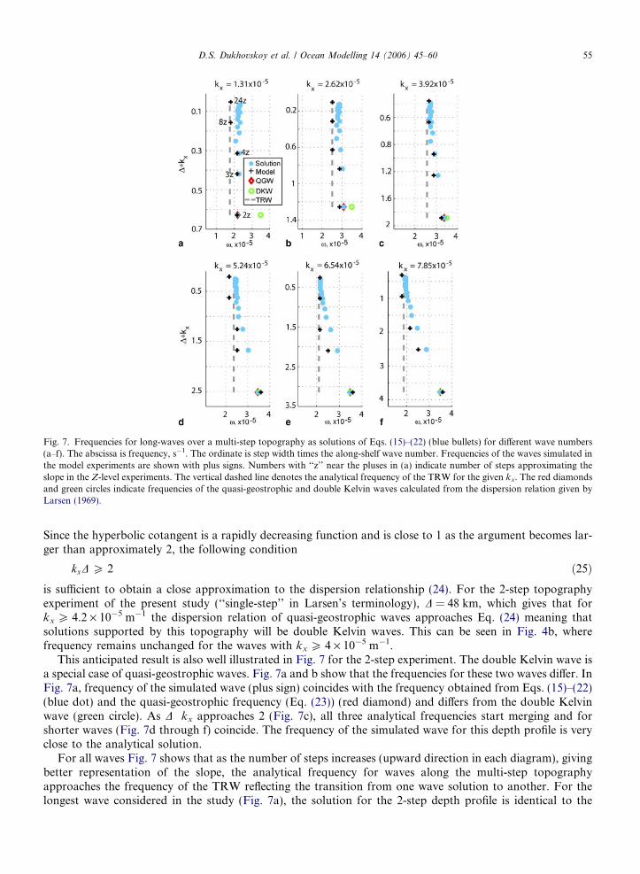
Fig. 7. Frequencies for long-waves over a multi-step topography as solutions of Eqs. (15)–(22) (blue bullets) for different wave numbers(a–f). The abscissa is frequency, s�1. The ordinate is step width times the along-shelf wave number. Frequencies of the waves simulated inthe model experiments are shown with plus signs. Numbers with ‘‘z’’ near the pluses in (a) indicate number of steps approximating theslope in the Z-level experiments. The vertical dashed line denotes the analytical frequency of the TRW for the given kx. The red diamondsand green circles indicate frequencies of the quasi-geostrophic and double Kelvin waves calculated from the dispersion relation given byLarsen (1969).


Since the hyperbolic cotangent is a rapidly decreasing function and is close to 1 as the argument becomes lar-ger than approximately 2, the following condition

kxD P 2 ð25Þ
is sufficient to obtain a close approximation to the dispersion relationship (24). For the 2-step topographyexperiment of the present study (‘‘single-step’’ in Larsen’s terminology), D = 48 km, which gives that forkx P 4.2 · 10�5 m�1 the dispersion relation of quasi-geostrophic waves approaches Eq. (24) meaning thatsolutions supported by this topography will be double Kelvin waves. This can be seen in Fig. 4b, wherefrequency remains unchanged for the waves with kx P 4 · 10�5 m�1.
This anticipated result is also well illustrated in Fig. 7 for the 2-step experiment. The double Kelvin wave isa special case of quasi-geostrophic waves. Fig. 7a and b show that the frequencies for these two waves differ. InFig. 7a, frequency of the simulated wave (plus sign) coincides with the frequency obtained from Eqs. (15)–(22)(blue dot) and the quasi-geostrophic frequency (Eq. (23)) (red diamond) and differs from the double Kelvinwave (green circle). As D Æ kx approaches 2 (Fig. 7c), all three analytical frequencies start merging and forshorter waves (Fig. 7d through f) coincide. The frequency of the simulated wave for this depth profile is veryclose to the analytical solution.

For all waves Fig. 7 shows that as the number of steps increases (upward direction in each diagram), givingbetter representation of the slope, the analytical frequency for waves along the multi-step topographyapproaches the frequency of the TRW reflecting the transition from one wave solution to another. For thelongest wave considered in the study (Fig. 7a), the solution for the 2-step depth profile is identical to the


quasi-geostrophic wave frequency. For smaller steps, the solutions for multi-step depth profiles do not changeappreciably due to the fact that the step size is always small compared to k�1

x . The solutions stay close to thefrequency of the TRWs and do not show any dependence on the number of steps. Frequencies of the simulatedwaves become nearly identical to the theoretical value (dashed line) for well-resolved bathymetry (8 and 24steps). The waves presented in Fig. 7b show similar behavior; however, the solutions reveal some dependenceon the number of steps and approach the theoretical frequency as the number of Z levels increases. Startingwith Fig. 7c, the multi-step solutions appear identical to the frequencies of the TRWs when the conditionD Æ kx < 0.5 is satisfied. Frequencies of the simulated waves (plus signs) in all cases exhibit the same tendency,shifting from higher frequencies to lower and approaching the TRW frequency as D Æ kx decreases.

5.3. Some notes on the double Kelvin wave

A noticeable feature of the waves over a multi-step topography, noticed earlier in Fig. 4, is the transforma-tion of dispersive TRWs into nondispersive waves, double Kelvin waves. From Fig. 4 one may see that thefrequencies of the waves for 2- and 3-step topographies (Fig. 4b and c) do not change noticeably. The reasonbecomes clear if the dispersion relation of a wave trapped along a topographic discontinuity is examined.Following Longuet-Higgins (1968b), the sea surface displacement along the discontinuity is given by (seeFig. 8 for details)

g / g0ðyÞ exp½iðkxx� xtÞ�; ð26Þ
where
g0ðyÞ /expðky;1yÞ; y < 0;

expð�ky;2yÞ; y > 0:

�ð27Þ

Matching fluxes normal to the escarpment gives

h1ðxky;1 þ kxf Þ ¼ h2ð�xky;2 þ kxf Þ; ð28Þ
resulting in the dispersion relation
x ¼ dhkxfh1ky;1 þ h2ky;2

; ð29Þ

where dh = (h2 � h1). The value k�1y is a trapping scale that determines the rate of decay for the exponential

wave profile trapped along the escarpment. The wave number ky satisfies (Longuet-Higgins, 1968b)

ky ¼ k2x �

x2

ghþ f 2

gh

� �1=2

. ð30Þ

For subinertial waves which are the focus of the present study, x2� f2. Finally, the dispersion relation (29)becomes

Fig. 8. Schematic of a double Kelvin wave over a single-step topography.

Fig. 9. Schematic of the interaction of double Kelvin waves over multi-step topography. (a) The step is about 2 trapping distances wide sothat double Kelvin waves appear at the step edges. (b) The steps are narrow ðD� k�1

x ) and solutions at the edges merge together forming asingle waveform in the cross-shelf direction.


x ¼ dhkxf

h1 k2x þ

f 2

gh1

� 1=2

þ h2 k2x þ

f 2

gh2

� 1=2. ð31Þ

From (31) follows that for short waves ðk2x � f 2=ghÞ the dispersion relation becomes the nondispersive one

for double Kelvin waves given in Eq. (24). Also from Eq. (30), jkxj � jkyj and the trapping scale becomes k�1x

for the frequencies of interest. A scale estimate for the condition for short waves yields that the double Kelvinwave should be observed for kx > O(1 · 10�6). So this confirms that the simulated waves are the double Kelvinwaves whenever (25) is satisfied, since for all the waves in the study kx > 1 · 10�5.

It should be noted that the above discussion holds only for a single-step case which is applicable to themulti-step case only when condition (25) is satisfied, i.e. the step is at least two trapping distances wide (seeFig. 7c–f). In this case the steps are wide enough to allow the existence of double Kelvin waves along the stepedges (Fig. 9a). As the steps become smaller, the waveform solutions at adjacent step edges can merge and awaveform can potentially span over multiple steps (Fig. 9b) as seen in the numerical and analytical modelswith D Æ kx < 2.

5.4. Further remarks

In the previous discussion most attention has been paid to the horizontal dimension of the steps approx-imating the slope rather than to their vertical size. The width and the height of the steps formed by verticalZ levels are related to each other and both are the functions of the horizontal and vertical resolutions. A num-ber of experiments with Z-level models of varying vertical resolution and e-folding scale of bathymetry (notpresented) has shown that the ability of the model to reproduce different types of topographic waves is mostlysensitive to the width of the steps and less to the height of the step (to a certain degree). The above analysis ofanalytically derived frequencies satisfying the dispersion relationship (15) of a long wave over a multi-steptopography shows that the wave solutions transform into TRWs for D Æ kx 6 0.5. This means that the widthof the steps approximating the bathymetry should be less than half the trapping scale of the wave. For exam-ple, for a topographic wave with the along-shelf wave number kx = 1.26 · 10�5 m�1 ( kx = 500 km), the stepwidth needs to be <40 km to provide a fairly accurate propagation of the TRW in a Z-level model.

6. Summary

The main goal of this study is to investigate the effect of multi-step topography on the propagation of topo-graphic waves. At the same time, this study addresses the question of whether Z-level models are able to sup-port TRWs and how the vertical grid spacing should be chosen to allow the model to accurately simulateTRWs of a given wavelength over a given topographic slope. The ability of ocean models with Z-level verticalgrids to simulate TRWs has been examined using the NCOM as a numerical tool. A simple case of abarotropic ocean on the f-plane over a long shelf with exponential depth profile is investigated. A series of


numerical experiments with varying numbers of Z levels, resulting in varying numbers of steps approximatingthe slope, are performed. In all experiments, the model is initialized with analytical velocity and SSH fields forthe varying along-shelf wave numbers. The solutions are compared to the control run performed using NCOMwith 1r level and dispersion relationships obtained from the model experiments are compared to the analyticalrelations.

Two different types of topographic waves have been simulated by the experiments using different numbersof Z levels. At the limiting case with very coarse vertical resolution resulting in wide and high steps, the modelproduces double Kelvin waves which are trapped waves trapped along the step edges. The existence of thistype of wave in the models with poor vertical discretization is possible due to wide steps formed by rounding(or truncation) of the bathymetry to the Z-level vertical grid. Analysis of dispersion relationships estimated forthe simulated waves and analytically derived for multi-step topography has revealed that the quasi-geostrophic waves convert to double Kelvin waves when D Æ kx becomes larger than 2. In other words, doubleKelvin waves are supported when the step width is on the order of two trapping distances of the wave orlarger. As the step width becomes smaller the wave solutions at the step edges start merging producing a wavesolution that spans over several steps. As the steps become small (roughly less than one-half) compared to thetrapping scale k�1

x , the simulated waves are similar to the TRW seen in the control run in terms of waveforms(Fig. 3) and their dispersion relationship (Fig. 4). Analytically derived frequencies for a multi-step depthprofile (Fig. 7) illustrate how the wave solution transforms from a double Kelvin wave for very coarse verticaldiscretization to a TRW-like wave when the steps becomes small.

These results demonstrate the ability of a Z-level model to simulate TRWs. Knowing a characteristic lengthof the TRW expected to occur and the depth profile in the region of interest, the number of Z levels should besuch that the width of the steps approximating the slope is less than one-half the trapping scale, D Æ kx 6 0.5.When D Æ kx P 0.5 the frequency of the wave propagating in the Z-level model drifts toward higher values asD Æ kx increases. If a model is configured with too coarse vertical resolution so that D Æ kx P 2, the model won’tsupport TRWs, but rather double Kelvin waves which, being nondispersive, do not propagate energy withinthe domain. Thus, shorter topographic waves tend to be trapped along the step edges and longer waves tend toreveal TRW-like behavior for the same number of vertical Z levels. For a realistic ocean, this study shows thatbottom topography can significantly modify topographic wave characteristics. A bottom profile with large dis-continuities (steps) will split a wave into several trapped waves traveling along the step edges. If the width ofthe bottom steps is less than half of the trapping scale ðk�1

x Þ the wave will not feel the steps as discontinuitiesand will propagate as a TRW.

The significance of topographic waves (both barotropic and baroclinic) in climate variability has beenadvocated in a number of studies (Timmermann et al., 1998; Capotondi, 2000; Capotondi and Alexander,2001; Rossby and Nilsson, 2003). The correct simulation of the topographic waves could be important forclimate models as the waves are a major source of teleconnections throughout the ocean allowing the existenceof remote forcing. The present study might provoke further investigation of how accurately the GCMs (espe-cially those using Z-level models) simulate the TRWs.

Acknowledgements

This study was supported by the Office of Naval Research under the Secretary of Navy Grant toJ.J. O’Brien and NASA, Physical Oceanography. The authors would like to thank Paul Martin and AlanWallcraft at the Naval Research Laboratory for the NCOM development and assistance with the model.

References

Adcroft, A., Hill, C., Marshall, J., 1997. Representation of topography by shaved cells in a height coordinate ocean model. Month. Weath.Rev. 125, 2293–2315.

Ball, F.K., 1967. Edge waves in an ocean of finite depth. Deep-Sea Res. 14, 79–88.Beckmann, A., Doscher, R., 1997. A method for improved representation of dense water spreading over topography in geopotential-

coordinate models. J. Phys. Oceanogr. 27, 581–591.Bleck, R., 1998. Ocean modeling in isopycnic coordinates. In: Chassignet, E.P., Verron, J. (Eds.), Ocean Modeling and Parameterization.

Kluwer Academic Publishers, pp. 423–448.


Blumberg, A., Mellor, G.L., 1987. A description of a three-dimensional coastal ocean circulation model. In: Heaps, N. (Ed.), Three-Dimensional Coastal Ocean Models. Amer. Geophys. Union.

Brooks, D.A., Mooers, C.N.K., 1977. Free, stable continental shelf waves in a sheared, barotropic boundary current. J. Phys. Oceanogr. 7,380–388.

Bryan, K., 1969. A numerical method for the study of the circulation of the World Ocean. J. Comput. Phys. 4, 347–376.Capotondi, A., 2000. Oceanic wave dynamics and interdecadal variability in a climate system model. J. Geophys. Res. 105 (C1), 1017–1036.Capotondi, A., Alexander, M.A., 2001. Rossby waves in the tropical North Pacific and their role in decadal thermocline variability.

J. Phys. Oceanogr. 31 (12), 3496–3515.Clarke, A.J., Brink, K.H., 1985. The response of stratified, frictional flow of shelf and slope waters to fluctuating large-scale, low-

frequency wind forcing. J. Phys. Oceanogr. 15, 439–453.Cushman-Roisin, B., 1994. Introduction to Geophysical Fluid Dynamics. Prentice-Hall, New Jersey.Cushman-Roisin, B., O’Brien, J.J., 1983. The influence of bottom topography on baroclinic transports. J. Phys. Oceanogr. 13, 1600–1611.Flato, G.M., Boer, G.J., Lee, W.G., McFarlane, N.A., Ramsden, D., Reader, M.C., Weaver, A.J., 2000. The Canadian Centre for Climate

Modelling and Analysis global coupled model and its climate. Climate Dyn. 16.Gent, P.R., Bryan, F.O., Danabasoglu, G., Doney, S.C., Holland, W.R., Large, W.G., McWilliams, J.C., 1998. The NCAR climate system

model global ocean component. J. Climate 11 (6), 1287–1306. doi:10.1175/1520-0442.Gerdes, R., 1993. A primitive equation ocean circulation model using a general vertical coordinate transformation. 1. Description and

testing of the model. J. Geophys. Res. 98 (C8), 14683–14701.Gill, A., 1982. Atmosphere-Ocean Dynamics. Academic Press Inc., New York.Hamilton, P., Lugo-Fernandez, A., 2001. Observations of high speed deep currents in the northern Gulf of Mexico. Geophys. Res. Lett.

28, 2867–2870.Holland, W.R., Chow, J.C., Bryan, F.O., 1998. Application of a third-order upwind scheme in the NCAR Ocean Model. J. Climate 11,

1487–1493.Kara, A.B., Barron, C.N., Martin, P.J., Smedstad, L.F., Rhodes, R.C., 2005. Validation of interannual simulations from the 1/8� global

Navy Coastal Ocean Model (NCOM). Ocean Model. 1 (3–4), 376–398. doi:10.1016/j.ocemod.2005.01.003.Killworth, P.D., Stainforth, D., Webb, D.J., Paterson, S.M., 1991. The development of a free-surface Bryan–Cox–Semtner ocean model.

J. Phys. Oceanogr. 21, 1333–1348.Larsen, J.C., 1969. Long waves along a single-step topography in a semi-infinite uniformly rotating ocean. J. Mar. Res. 27, 1–6.LeBlond, P.H., Mysak, L.A., 1977. Trapped coastal waves and their role in shelf dynamics. In: Goldberg, E.D. (Ed.), The Sea, Marine

Modeling, vol. 6. John Wiley & Sons, New York, pp. 459–498.LeBlond, P.H., Mysak, L.A., 1978. Waves in the Ocean. Elsevier, New York, 602 pp.Longuet-Higgins, M.S., 1968a. Double Kelvin waves with continuous depth profiles. J. Fluid Mech. 34, 49–80.Longuet-Higgins, M.S., 1968b. On the trapping of waves along a discontinuity of depth in a rotating ocean. J. Fluid Mech. 31, 417–434.Lugo-Fernandez, A., Morin, M.M., 2004. Slope and roughness statistics of the Northern Gulf of Mexico seafloor with some

oceanographic implications. Gulf Mexico Sci. 1, 22–44.Marshall, J., Hill, C., Perelman, L., Adcroft, A., 1997. Hydrostatic, quasi-hydrostatic and non-hydrostatic ocean modeling. J. Geophys.

Res. 103, 5733–5752.Martin, P.J., 2000. A description of the Navy Coastal Ocean Model Version 1.0. NRL Report: NRL/FR/7322-009962, Naval Research

Laboratory, Stennis Space Center, MS, p. 39.Martin, P.J., Peggion, G., Yip, K.J., 1998. A comparison of several coastal ocean models, Report: NRL/FR/7322-97-9672, Navy Research

Laboratory, Stennis Space Center, MS, p. 96.Mitchum, G.T., Clarke, A.J., 1986. Evaluation of frictional, wind forced long wave theory on the West Florida shelf. J. Phys. Oceanogr.

16, 1029–1037.Munk, W., Snodgrass, F., Gilbert, F., 1964. Long waves on the continental shelf: an experiment to separate trapped and leaky modes.

J. Fluid Mech. 20, 529–554.Nakano, H., Suginohara, N., 2002. A series of middepth zonal flows in the Pacific driven by winds, J. Phys. Oceanogr. 32 (1), 161–176.Pacanowski, R.C., Gnanadesikan, A., 1998. Transient response in a Z-level ocean model that resolves topography with partial cells.

Month. Weath. Rev. 126, 3248–3270.Pedlosky, J., 1987. Geophysical Fluid Dynamics. Springer, New York, 710 pp.Pickart, R.S., 1995. Gulf Stream-generated topographic Rossby waves. J. Phys. Oceanogr. 25, 574–586.Rhines, P.B., 1969. Slow oscillations in an ocean of varying depth. Part I. Abrupt topography. J. Fluid Mech. 37, 161–189.Roberts, M.J., Banks, H., Gedney, N., Gregory, J., Hill, R., Mullerworth, S., Pardaens, A., Rickard, G., Thorpe, R., Wood, R., 2003.

Impact of an eddy-permitting ocean resolution on control and climate change simulations with a global coupled GCM. J. Climate 17(1), 3–20. doi:10.1175/1520-0442.

Robinson, A.R., 1964. Continental shelf waves and the response of sea level to weather systems. J. Geophys. Res. 69, 367–368.Rossby, T., Nilsson, J., 2003. Current switching as the cause of rapid warming at the end of the last Glacial Maximum and Younger

Dryas. Geophys. Res. Lett. 30 (2), 1051. doi:10.1029/2002GL015423.Sandstrom, H., 1969. Effect of topography on propagation of waves in stratified fluids. Deep-Sea Res. 16, 405–410.Saunders, P.M., Coward, A.C., de Cuevas, B.A., 1999. Circulation of the Pacific Ocean seen in a global ocean model (OCCAM).

J. Geophys. Res. 104 (C8), 18281–18299.Song, Y.T., Chao, Y., 2000. An embedded bottom boundary layer formulation for Z-coordinate ocean models. J. Atmos. Ocean. Technol.

17, 546–560.

http://dx.doi.org/10.1175/1520-0442

http://dx.doi.org/10.1016/j.ocemod.2005.01.003

http://dx.doi.org/10.1175/1520-0442

http://dx.doi.org/10.1029/2002GL015423


Steiner, N., Holloway, G., Gerdes, R., Hakkinen, S., Holland, D., Karcher, M., Kauker, F., Maslowski, W., Proshutinsky, A., Steele, M.,Zhang, J., 2004. Comparing modeled streamfunction, heat and freshwater content in the Arctic Ocean. Ocean Model. 6 (3–4), 265–284.

Thompson, R.O.R.Y., 1971. Topographic Rossby waves at a site north of the Gulf Stream. Deep-Sea Res. 18, 11–19.Timmermann, A., Latif, M., Voss, R., Grotzner, A., 1998. Northern hemispheric interdecadal variability: a coupled air–sea mode.

J. Climate 11 (8), 1906–1931. doi:10.1175/1520-0442.Volterra, V., 1887. Sopra le funzioni dipendenti da linee. Rendiconti della R. Acc. Naz. dei Lincei 3 (4), 225–274.Volterra, V., 1959. Theory of Integral and Integrodifferential Equations. Dover, New York.Wang, D.-P., Mooers, C.N.K., 1976. Coastal-trapped waves in a continuously stratified ocean. J. Phys. Oceanogr. 6, 853–863.Zhang, J., Rothrock, D.A., 2003. Modeling global sea ice with a thickness and enthalpy distribution model in generalized curvilinear

coordinates. Month. Weath. Rev. 131, 845–861.Zhang, Y.X., Maslowski, W., Semtner, A.J., 1999. Impact of mesoscale ocean currents on sea ice in high-resolution Arctic ice and ocean

simulations. J. Geophys. Res. 104 (C8), 18409–18429.

http://dx.doi.org/10.1175/1520-0442

inﬂuence of multi-step topography on barotropic waves and...

Documents