Introductory Laboratory Course Physics

Part I (Winter term)

The Greek alphabet

Name Minuskel Majuskel Alpha α A Beta β B Gamma γ Γ Delta δ ∆ Epsilon ε E Zeta ζ Z Eta η H Theta θ Θ Iota ι I Kappa κ K Lambda λ Λ My µ M Ny ν N Xi ξ Ξ Omikron o O Pi π Π Rho ρ P Sigma σ Σ Tau τ T Ypsilon υ Y Phi ϕ Φ Chi χ X Psi ψ Ψ Omega ω Ω

Carl von Ossietzky Universität Oldenburg, Fakultät V, Institut für Physik, D-26111 Oldenburg Tel.: 0441-798-3395 (Technical Assistants) / 3153 (Laboratory Manager)

Internet: http://physikpraktika.uni-oldenburg.de

michael.krueger@uni-oldenburg.de

October 2016

(Translated by Christian Schöne, Angelika Sievers, Liz von Hauff, and Julika Mimkes)

Pictures on the title page: Top: Karman vortex street behind a cylinder of approx. 6 mm diameter. The photo shows an area of approx. 2.5 cm

× 7 cm. ©: AG Applied Optics, Institute of Physics, Carl von Ossietzky Universität Oldenburg Center: Karman „cloud street“ behind the Jan Mayen island (Norway), caused by the volcano Beerenberg of approx.

2.2 km height in the centre of the island. The photo shows an area of approx. 365 km × 158 km. ©: NASA; http://photojournal.jpl.nasa.gov/tiff/PIA03448.tif

Bottom: Flow vortices in the atmosphere of the planet Jupiter in the vicinity of the Great Red Spot. In front of Jupiter his moon Io (diameter 3.643 km), which throws its shadow on the surface of the planet. ©: NASA; http://ppj-web-3.jpl.nasa.gov/jpegMod/PIA02860_modest.jpg

1

Carl von Ossietzky University Oldenburg – Faculty V - Institute of Physics Module Introductory laboratory course physics – Part I

Contents Contents 1 Succession of experiments 2 Measurement of ohmic resistances, bridge circuits, and internal resistances of voltage sources 3 Measurement of capacities – Charging and discharging of capacitors 18 Sensors for force, pressure, distance, angle and light intensity 33 Force, momentum and impulse of force 47 Data acquisition and data processing using a PC 57 Characterization of a transreceiver system 71 Conservation of momentum and energy - Law of collision 80 Moment of inertia - Steiner's theorem 91 Forced mechanical oscillations 98 Fourier analysis 111 Surface tension, minimal surfaces, and coffee stains 122 Viscosity and Reynolds numbers 132 Translation of German denotations in figures of the script 145

2

Carl von Ossietzky Universität Oldenburg – Faculty V - Institute of Physics Module Introductory laboratory course physics – Part I

Succession of the experiments

Schedule Week Presen-tation Subject

1 42

General remarks on the module Introductory Laboratory Course Physics, the preparation of reports, and the usage of computers. Exercises to Origin and Matlab (Introductory Script)

2 43 Oscilloscope and function generator (Introductory Script)

3 44 Measurement of ohmic resistances, bridge circuits, and internal resistances of voltage sources

4 45 Measurement of capacities – Charging and discharging of capacitors (Extra seminar: Error theory I)

5 46 Sensors for force, pressure, distance, angle and light intensity (Extra seminar: Error theory II); Excercises in error theory

6 47 Force, momentum and impulse of force

7 48 Data acquisition and data processing using a PC

8 49 Characterization of a transreceiver system

9 50 Conservation of momentum and energy - Law of collision

10 51 Moment of inertia - Steiner's theorem

11 2 Forced mechanical oscillations

12 3 Fourier analysis

13 4 Surface tension, minimal surfaces and coffee stains

14 5 Viscosity and Reynolds numbers

The first experiments performed in the introductory laboratory course physics serve to become acquainted with measuring instruments, function generators, sensors and data acquisition as well as data processing using a PC and to carry out introductory quantitative measurements. Only part of the subjects treated in these experiments are dealt with in the lecture, too. A sound school knowledge of physics, however, will do all right to understand them. The following experiments are thematically coupled to the lecture contents that are dealt with synchronously. An Open Lab is offered at a time announced on the notice-board of the laboratory course. During this time the labs are opened and the devices are placed at the students' disposal. By this, the possibility is offered to the students to deepen and improve experimental abilities independently and to repeat experiments if necessary. Supervision is done in turns by one of the supervisors and technical assistants.

3

Carl von Ossietzky University Oldenburg – Faculty V - Institute of Physics Module Introductory laboratory course physics – Part I

Measurement of Ohmic Resistances, Bridge Circuits and Internal Resistances of Voltage Sources

Keywords: OHM's law, KIRCHHOFF's laws (KIRCHHOFF's current and voltage laws), internal resistances of meas-uring instruments, WHEATSTONE bridge, bridge circuit, voltage source, internal resistances of voltage sources, terminal voltage, strain gauge.

Measuring program: Measurement of resistances with different ohmmeters, determination of a resistance by means of a current / voltage measurement, WHEATSTONE bridge, internal resistance of a function generator, specific resistance of tap water, bridge circuit for measuring alterations to resistances.

References:

/1/ SCHENK, W., KREMER, F. (HRSG.): „Physikalisches Praktikum“, Vieweg + Teubner Verlag, Wiesbaden /2/ WALCHER, W.: „Praktikum der Physik“ Teubner Studienbücher, Teubner-Verlag, Stuttgart /3/ EICHLER, H.J., KRONFELDT, H.-D., SAHM, J.: „Das Neue Physikalische Grundpraktikum”, Springer-Verlag,

Berlin among others

1 Introduction

In the first part of this experiment, an insight into the different methods of measuring ohmic1 resistances will be given. In particular, it will be shown to which degree real properties of measuring instruments affect the results of a measurement, and which methods yield the best results in individual cases. In the second part of the experiment, the characteristics of real voltage sources are investigated. The main question here is how an important characteristic of such voltage sources, namely their internal resistance, can be measured. Additionally, the specific resistance of tap water is measured, and the linear relationship between changes in resistance and voltage in a bridge circuit is analysed.

2 Theory

2.1 Kirchhoff's Laws Knowledge of KIRCHHOFF's laws2 is a prerequisite for analysing electric networks (circuits) (see Fig. 1). KIRCHHOFF´s first law (current law) reads:

The sum of all currents at a branch point equals zero. For this law the sign convention is valid that currents towards and off a network node are marked by con-trary signs. It is of no importance, whether the affluent currents are marked positively and the effluent currents are marked negatively. Applied to the circuit in Fig. 1, KIRCHHOFF’s first law at the nodes A and B reads as follows:

(1) 1 2 3 2 3 1A : 0 B : 0I I I I I I− − = + − =

1 Named after GEORG SIMON OHM (1789 - 1854) 2 GUSTAV ROBERT KIRCHHOFF (1824 – 1887)

4

Fig. 1: Circuit with a direct voltage source with terminal voltage U, the resistorsR1,...,R3 as well as two nodes A

and B and two loops a and b. KIRCHHOFF´s second law (voltage law) reads:

In a closed loop of a network the sum of all components of the voltage equals zero. For the application of this law a sign convention is essential as well. It reads:

a) A direction („counting arrow”) is assigned to each voltage running from the positive to the negative terminal (e.g. voltage source).

b) A direction („counting arrow”) is assigned to each current, which marks the direction of movement

of the positive charge carriers, i.e., the current flows from the positive to the negative pole per definition. According to OHM’s law, the direction of the voltage UR over a resistance R corresponds to the direction of the current IR, flowing through R and causing the voltage drop UR.

c) For the application of the voltage law a direction of rotation has to be fixed (i.e., clockwise or

counter-clockwise). Voltages with counting arrows corresponding with the direction of rotation are counted as positive, the others as negative.

Applied to the circuit in Fig. 1, the KIRCHHOFF’s second law in the loops a and b for a counter clockwise direction of rotation reads:

(2) 2 1 2 3a : 0 b : 0U U U U U− − = − = With KIRCHHOFF’s two laws and the related sign conventions all electric networks which are employed in the course of the introductory laboratory course can be described. Question 1: - How can the formulas for the parallel and series connection of ohmic resistances be derived from

KIRCHHOFF's laws? Which are the corresponding relationships? It is not always easy to recognize whether resistances and other components in a network are in parallel or in series connections. Two rules derived from KIRCHHOFF's laws can be useful in making that decision: Resistances are in parallel if they show the same voltage drop. Resistances are in series if the same current flows through them.

2.2 Methods for Measuring Ohmic Resistances 2.2.1 Determining the Resistance from the Markings Fig. 2 depicts some common retail versions of resistors which are labeled with various kinds of markings (letterings or color codes). In the simplest case, the value of the resistor is printed directly on the casing. Some inscriptions commonly used for this purpose are “120R” for 120 Ω, “4R7” for 4.7 Ω, “3k3” for 3.3 kΩ, or “5M6” for 5.6 MΩ.

R

R R

1

2 3U

A

a b

I , U1

+ _

1

B

I , U3 3I , U2 2

5

Fig. 2: Common retail versions of resistors with various types of markings. Top load resistors (power rating of several W), bottom resistors for low power applications (< 1 W).

Equally simple is reading the colour key printed on most types of resistors. This colour key on the resistor consists of chromatic rings, which are always arranged in such a way that the first chromatic ring is closer to the one end of the resistor than the last chromatic ring is to the other end. Table 1 shows how the value of a resistance can be determined by means of the colour coding.

3 - 4 rings 1st ring 2nd ring 3rd ring 4th ring 5 - 6 rings 1st ring 2nd ring 3rd ring 4th ring 5th ring 6th ring Colour ↓ 1st number 2nd number 3rd number Multiplier / Ω Tolerance / % Temp. coeff. / 10-6ΩK-1

black 0 0 1 ± 250 brown 1 1 1 10 ± 1 ± 100

red 2 2 2 102 ± 2 ± 50 orange 3 3 3 103 ± 15 yellow 4 4 4 104 ± 25 green 5 5 5 105 ± 5*) ± 20 blue 6 6 6 106 ± 10 violet 7 7 7 107 ± 5 grey 8 8 8 10-2*) ± 1 white 9 9 9 10-1*) ± 10*) none ± 20 silver 10-2 ± 10 gold 10-1 ± 5

*) where the conductivity of gold and silver enamel interferes

Table 1: Colour key for ohmic resistances. Question 2: - What is the value of a resistor for the colour coding Red (first ring) - Violet - Brown - Gold? - What is the colour coding for a resistor of (3.9 kΩ ± 10 %)?

2.2.2 Determining the Resistance by Means of a Current / Voltage Measurement When the two ends of an ideal voltage source (cf. Chapter 2.3), which delivers an adjustable terminal voltage U, are connected with the connecting wires of a resistor R, the current I flows through the resistor and OHM’s law reads:

(3) R UI

=

6

By measuring the voltage U using a voltmeter and the current I using an ammeter, R can thus be determined. Such a measurement can be carried out using the two circuits A and B according to Fig. 3.

Fig. 3: Two possible circuits for measuring the resistance R by means of a current/voltage measurement. R is connected with a direct voltage source with terminal voltage U. The current is measured with the ammeter A, the voltage is measured with the voltmeter V.

If ideal measuring instruments were available, i.e., ammeter with a negligible internal resistance and a voltmeter with an infinitely high internal resistance, both circuits would yield the same result. However, an ammeter has an internal resistance of RA > 0 and a voltmeter has an internal resistance of RV < ∞. Con-sequently, a value for the resistance R with an error ∆R is determined with each circuit. We will now determine the relative error ∆R/R for both circuits. Let IA be the current through the ammeter, IR the current through the resistor, and IV the current through the voltmeter. UA is the voltage drop across the ammeter, UR is the voltage drop across R and UV is the voltage drop across the voltmeter. According to KIRCHHOFF's current law we then obtain for the circuit A: (4) I I IA R V− − = 0 and thus

(5) VRA III += Using this circuit, the value determined for the resistor RM is given by

(6) V VM

A R V

U UR

I I I= =

+

The deviation ∆R from the actual value R

(7) R UI

R

R

=

is hence given by: (8) ∆R R RM= − Inserting Eq. (6) into Eq. (8) and using circuit A, we obtain after some rearrangement and taking into consideration UV = UR (voltage law) for the relative error:

(9) VRR

RRR

+=

∆

According to KIRCHHOFF's voltage law we obtain for circuit B: (10) U U UV A R− − = 0

V

Schaltung A

U

A

R V

Schaltung B

UR

AI , UA A

I , UV VI , UR R I , UV V

I , UA A

I , UR R

+ _

+ _

7

and thus (11) U U UV A R= + Considering IA = IR, the measured resistance RM is:

(12) RRI

UUI

UI

UR AA

RA

R

V

A

VM +=

+===

For the actual resistance R we refer again to Eq. (7). Inserting Eq. (12) into Eq. (8), we obtain for the relative error, if using circuit B:

(13) ∆RR

RR

A= −

Question 3: - Sketch the graph of the relative error as a function of the resistance R for circuits A and B in a diagram.

Is one of the circuits better than the other one, in principle? If not: in which case would the individual circuits be preferred?

- The two circuits are called „current-correct” and „voltage-correct” circuits, respectively. Which name belongs to which circuit? Why?

2.2.3 Measurement of Resistance Using an Ohmmeter Instead of determining the resistance from a current/voltage measurement, it can also be directly measured using an analogous ohmmeter (pointer instrument). In the simplest case such an ohmmeter consists of a voltage source (battery), to which the resistance R is connected, a variable internal resistance Ri and an ammeter, by means of which the current through the resistance R is determined. This current causes a needle deflection, which is then read off an appropriate OHM scale. This scale is inversely proportional to the current scale due to the relationship R = U/I. Since the voltage source does not always provide the same voltage (ageing of battery), the ohmmeter has to be calibrated by adjusting Ri before beginning the measurement. For this purpose the contacts are shorted out and the needle deflection is adjusted to 0 Ω using a regulating screw. Modern digital ohmmeters are structured differently. Generally, they are integrated into multimeters. Such instruments contain complex electronic circuits with integrated microprocessors for measuring the required parameters (current, voltage, resistance, frequency among others) and LCD elements displaying the measured values.

2.2.4 Measurement of Resistance Using the WHEATSTONE Bridge By means of a WHEATSTONE bridge3 the value of a resistance R can be determined without errors being caused by inadequate (real) measuring instruments for the current, voltage or resistance; however, a gauged comparative resistance is required for this purpose. We consider a WHEATSTONE bridge-circuit like the one in Fig. 4. A homogenous resistance wire, usually of constantan4 with the specific resistance ρ ([ρ] = Ωm), the total length l = l1 + l2, and the cross-sectional area A is connected to the resistor R to be measured and a gauged comparative resistor R3 as shown in the figure. The resistances of the two wires are:

(14) 1 21 2and

l lR R

A Aρ ρ= =

3 CHARLES WHEATSTONE (1802 – 1875) 4 Constantan is an alloy consisting of approx. 60 % copper and approx. 40 % nickel, the specific resistance of which is nearly

constant across a wide temperature range (ρ ≈ 45 × 10-8 Ωm at 20 °C).

8

The voltage U, taken from a direct-voltage source, is connected to this resistance network. The current flowing between the point P and the shiftable tapping point Q along the resistance wire is measured using an ammeter A.

Fig. 4: Wheatstone bridge with constantan resistance wire (yellow). R (green) is the resistor to be measured, R3 is the resistor used for comparison.

There is a position of the tapping point Q, where no voltage is found between P and Q and therefore no current flows. In that case the voltages over R3 and R1 as well as at R and R2 are equal. Such a WHEATSTONE bridge is called „adjusted” and we obtain:

(15) 3 1 1

2 2

R R lR R l

= =

and thus

(16) 23

1

lR Rl

=

Thus, in the case of an adjusted WHEATSTONE bridge, the resistance R can be determined by measuring the lengths l1 and l2 and knowing the gauged resistance R3 from Eq. (16); insufficiencies of electric instruments are then of no importance. This is the advantage of this measuring method, a so-called compensation method. Question 4: - In Fig. 4, enter all the points where the circuit branches in the unbalanced WHEATSTONE bridge as well

as the currents that flow, including their signs. - In Fig. 4, draw all of the loops of the unbalanced WHEATSTONE bridge as well as the voltages in these

loops, including their signs.

2.2.5 Bridge Circuit for Measuring Alterations to Resistance Bridge circuits are, among other applications, used to convert small alterations to resistance ∆R into pro-portional voltages. This is a standard method in many areas of sensor-measuring-technology. We consider, for example a bridge circuit with strain gauges (SG). SGs may be used for constructing force sensors. We will get to know such a force sensor in the experiment “Sensors...”. Its theoretical foundation, however, shall already be described here. The principle of a strain gauge is the elongation of a thin electrical conductor of length l by means of an external force F5, which simultaneously causes a decrease of its cross-sectional area A (Fig. 5). This alters its resistance R, which is, according to Eq. (14), given by:

(17) lRA

ρ=

5 A positive elongation is a stretching, a negative one a compression.

U1l

R1

2lQ

R3

A

P

R2

R

+ _

9

Fig. 5: Diagram of a strain gauge (SG) on metal foil basis. A thin metal foil (yellow) is plated on the carrier foil

(gray) in meander form in order to increase the effective length of the conductor while keeping the size of the SG small. The carrier foil is pasted on the work piece to be investigated and follows its deformations upon application of a force F.

For a conductor with a circular cross-section of diameter d we get:

(18) 2

4π

lRd

ρ=

The elongation changes the length l by Δl, the diameter d by Δd, and, depending on the material, possibly the specific resistance ρ by Δρ. The resulting change in the ohmic resistance is given by the total differential ΔR:

(19) 2 2 3

1 4 4 42π

R R R l lR l d l dl d d d d

ρ ρ ρ ρρ

∂ ∂ ∂ ∆ = ∆ + ∆ + ∆ = ∆ + ∆ − ∆ ∂ ∂ ∂

The relative change in resistance is thus:

(20) 2R l dR l d

ρρ

∆ ∆ ∆ ∆= + −

The relative change in length ∆l/l is defined as the elongation ε.

(21) l

lε ∆

=

The POISSON-number6µ is defined as the negative quotient of the relative change of the cross section ∆d/d and the relative change of length ∆l/l, thus:

(22) :

d dd dl

l

µε

∆ ∆

= − = −∆

Factoring out the value of ε = Δl/l in Eq. (20) and substituting Eq. (21) and Eq. (22) into Eq. (20) gives:

6 SIMÉON DENIS POISSON (1781 – 1840)

F

10

(23) 1 2 :R kR

ρρ µ ε εε

∆ ∆ = + + =

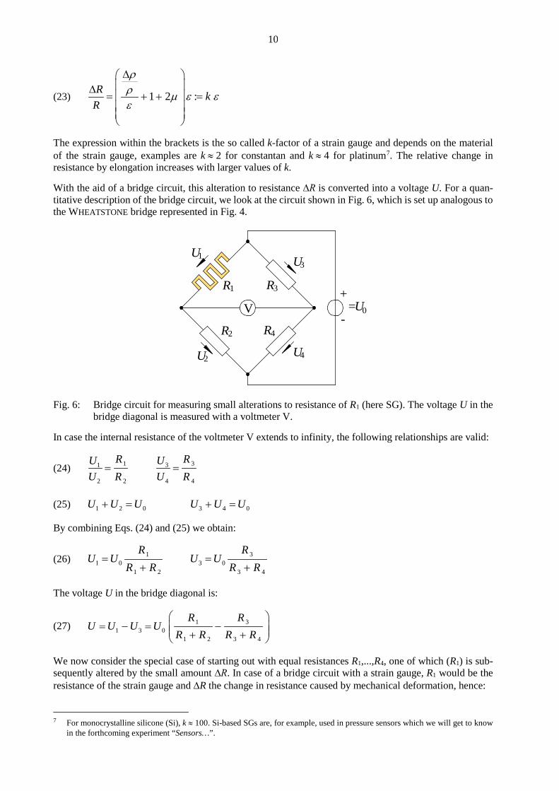
The expression within the brackets is the so called k-factor of a strain gauge and depends on the material of the strain gauge, examples are k ≈ 2 for constantan and k ≈ 4 for platinum7. The relative change in resistance by elongation increases with larger values of k. With the aid of a bridge circuit, this alteration to resistance ∆R is converted into a voltage U. For a quan-titative description of the bridge circuit, we look at the circuit shown in Fig. 6, which is set up analogous to the WHEATSTONE bridge represented in Fig. 4.

Fig. 6: Bridge circuit for measuring small alterations to resistance of R1 (here SG). The voltage U in the

bridge diagonal is measured with a voltmeter V. In case the internal resistance of the voltmeter V extends to infinity, the following relationships are valid:

(24) 1 331

2 2 4 4

R RUUU R U R

= =

(25) 1 2 0 3 4 0U U U U U U+ = + = By combining Eqs. (24) and (25) we obtain:

(26) 1 31 0 3 0

1 2 3 4

R RU U U U

R R R R= =

+ +

The voltage U in the bridge diagonal is:

(27) 1 31 3 0

1 2 3 4

R RU U U U

R R R R

= − = − + +

We now consider the special case of starting out with equal resistances R1,...,R4, one of which (R1) is sub-sequently altered by the small amount ∆R. In case of a bridge circuit with a strain gauge, R1 would be the resistance of the strain gauge and ∆R the change in resistance caused by mechanical deformation, hence: 7 For monocrystalline silicone (Si), k ≈ 100. Si-based SGs are, for example, used in pressure sensors which we will get to know

in the forthcoming experiment “Sensors…”.

V 0=UR1 R3

R4R2

+

-

U1

U2 U4

U3

11

(28) 1 2 3 4 :R R R R R R R= + ∆ = = = With this, it follows that the voltage U from Eq. (27) is given by:

(29) 00 0

1 12 2 2 2

UR R R R R RU U U RR R R R R R R RR

+ ∆ + ∆ ∆

= − = − = ∆+ ∆ + + + ∆ +

Eq. (29) shows that the relationship between U and ∆R is non-linear. If, however, ∆R << R, it holds:

(30) 1 1

22 RR

≈∆+

and thus:

(31) 0

4U RU

R∆

≈

Near the point of balance (∆R << R), the alteration to resistance ∆R is thus related to a voltage U in an approximately linear manner, the amplitude of which can be influenced by the operating voltage (supply voltage) of the bridge, U0. In the set-up described above, one of the four resistors is replaced by a SG. Accordingly, this setup is commonly called a quarter bridge. In practice, one often uses a bridge circuit where two resistors are replaced by SGs which move in opposite directions of each other for a given deformation (Fig. 7). This arrangement is called a half bridge. One example is using two SGs to measure forces with a bending rod (Fig. 8), which we will investigate in more detail in the experiment „Sensors...”. The two SGs are placed in the bridge circuit, so that the upper one that is being elongated replaces R1 and the lower one being compressed replaces R2. It follows that:

(32) 1 2 3 4R R R R R R R R R= + ∆ = − ∆ = =

Fig. 7: Bridge circuit with two SGs (half bridge).

V 0=UR1 R3

R4R2

+

-

U1

U2U4

U3

12

Fig. 8: Bending rod (green) with two strain gauges (yellow, German abbreviation is DMS). The rod (green) is fixed

by a block (gray) on the left. The force F deforms the rod, so that the upper SG is elongated and the lower one is compressed. A mechanical barrier (red) serves to protect the apparatus from overstraining.

By inserting Eq. (32) in Eq. (27), it follows for the half bridge:

(33) 0

2U RU

R∆

=

This equation makes the advantage of a half bridge compared to a quarter bridge clear: First, the relation between U and ∆R is linear. Second, for the same change in resistance ∆R, the half bridge produces an output voltage U of twice the magnitude. Thus, the sensitivity of the half bridge is twice as high.

In a full bridge, all four resistors are replaced by SGs, which change pairwise (R1/R4 and R2/R3) in opposite directions. In this case we find for the voltage U:

(34) 0RU U

R∆

≈

It is clear, that the sensitivity increases again by a factor of two.

2.3 Properties of Real Voltage Sources 2.3.1 Internal Resistance of Real Voltage Sources An ideal voltage source provides a constant terminal voltage U, which is equal to the constant source voltage U0, independently of the electrical load (the current it provides) at its connecting terminal. Such ideal voltage sources cannot be realized technically. On the contrary, we are dealing with real voltage sources such as batteries, power units or function generators, the terminal voltage of which decreases with increasing load. In order to describe this property of real voltage sources we use a model in which the real voltage source is exchanged for an ideal voltage source G and an internal resistance Ri in series; Fig. 9 shows the corresponding equivalent circuit. When such a voltage source is connected with a load with an external load resistance Rl according to Fig. 10, the load current I flows through Rl as well as through Ri. This current causes a voltage drop IRi at Ri by which the terminal voltage U is reduced compared to the source voltage U0. Thus we obtain: (35) U U IRi= −0

Fig. 9: Equivalent circuit of areal voltage source without a load.

Fig. 10: Equivalent circuit of a real voltage source with load resistance Rl .

F

DMS

0=UG

RiU

0

VR

=U G

iU Rl

I

13

If the source voltage U0 is to be measured using an ideal voltmeter V in a circuit according to Fig. 10, then the load current I has to be towards zero. This is achieved by a large load resistance Rl. Exchanging the current I in Eq.(35) for U/Rl (according to OHM's law) we obtain for the relationship between U and Rl:

(36) U U RR R

l

l i

=+0

From this equation we derive particularly for the case Rl = Ri that the terminal voltage decreases to half of the source voltage. This allows us to determine the internal resistance of a real voltage source. Question 5: - Sketch the graph of the terminal voltage U as a function of the load resistance Rl.

2.3.2 Matching a Device to a Real Voltage Source

2.3.2.1 Power Matching While connecting an electrical device to a voltage source it is often desirable that the internal resistance of the device be dimensioned such that the maximal power can be taken from the voltage source (power matching; applied e.g. in the transmission of high-frequency signals8). The internal resistance of the device is the load resistance Rl, which is the voltage source load. The power P supplied to that resistance is given by:

(37) P UI URl

= =2

Inserting Eq. (36) into Eq. (37) yields:

(38) ( )

P U RR R

l

l i

=+

02

2

Maximal power consumption is achieved when the internal resistance of the device equals the internal resistance of the voltage source, hence if we have: (39) R Rl i= Question 6: - Sketch the graph of P as a function of Rl. How do we get from Eq. (38) to Eq. (39)? What is the maximum

power that can be drawn from the voltage source?

2.3.2.2 Voltage Matching The object of voltage matching, applied in high-current technology and in sound engineering, is to draw the highest possible voltage U from the voltage source. According to Eq. (36) the necessary condition for this is: (40) R Rl i>>

2.3.2.3 Current Matching The object of current matching is to draw the strongest possible current I from the voltage source. This is, for example, used for charging accumulators. According to the OHM’s law we obtain:

8 Power matching in communication engineering at the same time prevents spurious signal reflections, which will be examined

more closely in the experiment “Signal transfer…” (summer term).

14

(41) li RR

UI+

= 0

so that the condition for the strongest possible current reads: (42) R Rl i<< In this case the current is nearly independent of the load resistance.

3 Experimental Procedure

Equipment: Voltage supply (PHYWE (0 - 15 / 0 - 30) V), function generator (TOELLNER 7401), several digital mul-timeters, digital oscilloscope TEKTRONIX TDS 1012 / 1012B / 2012C / TBS 1102B, resistance decade, slide rheostat (Rges ≈ 11,5 Ω), unknown resistance in holder, box for bridge circuit, pair of copper plates in holder, water basin on vertically adjustable holder, metal measuring tape, calliper gauge, paper wipes.

Attention:

When connecting resistances with voltage sources it has to be considered that the maximally allowable dissipation power Pmax of the resistor must not be exceeded (P = UI = U2/R < Pmax). Details about the load capacity Pmax of resistors are either found on the available components (e.g. resistor decade) or can be obtained from the technical assistant.

Take care when operating the power supply unit that no unintentional current limitation is adjusted.

Multimeters of the type FLUKE 112 provide only a limited resolution for current measurements. Therefore, they are used only as ohmmeters or voltmeters in this experiment, not as ammeters. In multimeters of the type MONACOR DMT-3010, fuses are blown easily in case of an operating error. Apply special caution to operating them!

3.1 Hints to the Measuring Instruments The used measuring instruments offer the possibility to switch the measuring range manually and partly also automatically, which serves to indicate the measured value on the scale or numerical display of the measuring instrument with the highest possible accuracy. For example, using a digital voltmeter a voltage of 1.78 V will be indicated as 1.78 V in the measuring range „2 V”, but will be indicated as 2 V in the measuring range „200 V”. When switching the measuring range of an ammeter a precision resistor („shunt”) is added in parallel to the internal resistance of the instrument. This resistor is rated such that the current flowing through the ammeter remains just about the same for all measuring ranges. Analogously, when switching the measuring range of a voltmeter, a precision resistor is added in series to the internal resistance of the instrument, which is rated such that the voltage drop is just about the same for all measuring ranges of the voltmeter. Data on the internal resistances for measuring currents (RA) and for measuring voltages (RV), which are dependent on the measuring range, are available for some of the measuring instruments used in the intro-ductory laboratory course. Instead of an internal resistance RA, a voltage drop ∆U is often stated (e.g. 20 mV, 200 mV etc.). In this case RA = ∆U / Imax, Imax representing the maximum current in the adjusted measuring range. For other measuring instruments, there are no data available on the internal resistances RA and/or RV. In those cases it can be assumed that RV is so large (e.g. 10 MΩ) and RA is so small (e.g. 0,5 Ω) that their influence on the measurement result is negligible. Specifications of the total measurement error of a measuring instrument and the precision of a measured value, respectively, are found on the instruments or in the instrument manuals. These values generally

15

consist of two parts. Their first - most significant - part is stated in percent of the measured value. Their second part can be stated in percent of the measuring range or in units of the last decimal of the measured value. The following examples serve for explanation: 1.) A direct voltage of 2.348 V is measured with the multimeter FLUKE 112 in the measuring range

6.000 V. According to the manual the precision for this voltage range is: ± (0.7 % of the measured value + 0.003) V. For the mentioned example, the precision thus is ± (0.007 × 2.348+ 0.003) V = ± 0.019 V (rounded to two significant digits). This value is also the maximum error for the measured value.

2.) A direct voltage of 297.34 mV is measured with the multimeter AGILENT U1272A in the measuring range 300.00 mV. According to the manual the precision for this voltage range is: ± (0.05 % + 5). The percent value refers to the measured value, the “5” refers to the last shown digit of the measured value (here the 4 in 0.04 mV). The maximum error therefore is: ± (0.0005 × 297.34 + 0.05) mV = 0.20 V (rounded to two significant digits).

3.2 Measurement of Resistances The value of an unknown resistor R (in the order of magnitude of 1 kΩ) including the maximum error is to be determined by applying some of the methods described in Chapter 2.2. The following steps are to be taken consecutively: a) Measurement using different ohmmeters: The value of the resistance R is to be measured with at least

five ohmmeters. Partly also ohmmeters of the same type may be used. A number j is assigned to every ohmmeter. Prior to the measurements, the measuring instruments have to be adjusted to the measuring range that enables the most precise measurement to be made. The maximum error ∆Rj is given for each measured value Rj. The Rj are presented in a graph over j including error bars.

b) Measurement of current/voltage: As an example, circuit A is set up according to Fig. 3. A voltage

supply serves as the voltage source. Its internal resistance can be neglected for this measurement. For at least ten different voltages on the voltage supply the corresponding current is measured using an ammeter and the voltage using a voltmeter. Prior to these measurements, the range covering the values to be measured has to be considered and the measuring ranges have to be adjusted accordingly. For each pair of values (U, I) a resistance R = U/I is determined. Subsequently, the mean R and its standard deviation Rσ are calculated from these data. Subsequently, the measured voltage values U are plotted against the measured current values I in a diagram and the maximum errors of U and I are entered in the form of error bars. The parameters of the regression line through the measured points are calculated and the regression line is drawn into the diagram9. The slope of the regression line R (± σR) is a good estimate for the unknown resistance value. This estimate is compared with the previously found mean of R (± Rσ ) and it is checked, whether both methods yield comparable results.

c) WHEATSTONE bridge: A WHEATSTONE bridge is set up according to Fig. 4. Again a voltage supply

serves as the voltage source, and a resistance from a resistor decade as calibration resistance R3. This resistance is chosen to be about the same as the resistance to be measured: R. In that case l1 ≈ l2 is valid for an adjusted WHEATSTONE bridge and the error becomes minimal for determining R. The error of the value of R calculated using Eq. (16) is given by the maximum error.

Question 7: - How can we explain that the error becomes minimal for determining R in the case l1 ≈ l2? (Hint: Consider

the reading precision of the length scale!) 9 The calculation of the parameters of the regression line and its grafic representation are done using Origin. Hints are given

in the accompanying seminar.

16

After having determined the resistance by applying the different methods, all measured results from Chap. 3.2 are to be presented in a graph analogous to Chap. 3.2 a) and compared.

3.3 Measurement of Internal Resistance of a Function Generator With a circuit according to Fig. 10, the internal resistance (also called output resistance) of a function generator (FG) is to be determined. The equivalent circuit of the function generator consists of an ideal voltage source G and the internal resistance Ri (order of magnitude 50 Ω) in series. A sinusoidal voltage is adjusted at the function generator (amplitude UFG ≈ 4 V, frequency approx. 1 kHz) and initially a load resistance Rl = 100 kΩ and thus Rl >> Ri (resistance decade) is connected. The voltage amplitude U over Rl is measured using an oscilloscope. Its internal resistance of about 1 MΩ can be neglected. U0 ≈ UFG is valid for Rl = 100 kΩ with sufficient precision. Subsequently, the load resistance is reduced by correspondingly switching the resistor decade to values between 1 kΩ and 20 Ω. For each value of Rl, the voltage amplitude U is measured and subsequently U is plotted over Rl. By means of graphic interpolation10 of the curve the value for Rl is extrapolated at which U has been decreased to half of U0. This resistance corresponds to the required internal resistance Ri of the function generator (see Chapter 2.3.1). Hint:

The maximum current at the lowest possible resistance (20 Ω) is Imax = 4 V / 20 Ω = 200 mA. The maximum momentary power at the resistance thus is P =U I = 0.8 W and hence is below the load limit of the resistance decade of 1 W.

3.4 Specific Resistance of Tap Water Let us examine the set-up shown in Fig. 11. Two rectangular copper plates of width b are mounted in parallel at a distance l. They are dipped into a water basin containing normal tap water. By lifting the water basin the plates can be plunged into the water to a variable depth d. ρw being the specific resistance of the water, the ohmic resistance Rw of the water between the plates is given by (cf. Eq. (14)):

(43) w w1lR

b dρ=

Fig. 11: Set-up for measuring the specific resistance of tap water (ammeter and voltmeter not drawn). By measuring the current I (ammeter) at an applied voltage U (voltmeter) between the plates Rw (circuit A, cf. Fig. 3) is determined for a number of values of the immersion depth d, within the range between 50 mm and 20 mm. For the single values of U, I and Rw errors must not be specified. Then, Rw is plotted against

10 „Graphic interpolation“ means: A regression curve is drawn by hand through the measurement. Then the line U = U0/2 is drawn

and its intersection point with the regression curve is determined. The R value of the intersection point is read on the abscissa. Its maximum error ∆R follows from the reading accuracy of R.

d

l

U ~

17

1/d. A regression line is drawn in the diagram and the specific resistance ρw of the tap water including the maximum error is calculated from its slope (measure l and b!). Remarks:

In order to avoid polarization effects in the water, no direct voltage but a sinusoidal alternating voltage without DC offset (turn off “DC-Offset” on the FG) is used, which can be obtained from a function generator (Ueff ≈ 2 V at d ≈ 50 mm, frequency approx. 50 Hz). In spite of this, the water as an ionic conductor does not behave in the manner that we know from metallic conductors. For example, its resistance decreases with temperature, while for metallic conductors, it increases. Therefore, we must assume that the measurement yields only a reference value for ρW. In addition, ρw deviates considerably depending on the quality of the tap water, so we need not compare the measured value with a literature value.11

Measuring with an alternating voltage requires the multimeters to be switched into AC mode!

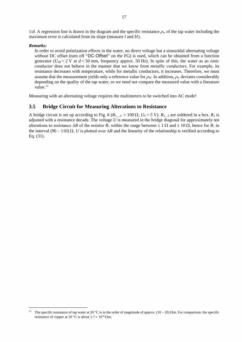
3.5 Bridge Circuit for Measuring Alterations to Resistance A bridge circuit is set up according to Fig. 6 (R1,...,4 ≈ 100 Ω, U0 ≈ 5 V). R2…4 are soldered in a box. R1 is adjusted with a resistance decade. The voltage U is measured in the bridge diagonal for approximately ten alterations to resistance ∆R of the resistor R1 within the range between ± 1 Ω and ± 10 Ω, hence for R1 in the interval (90 – 110) Ω. U is plotted over ∆R and the linearity of the relationship is verified according to Eq. (31).

11 The specific resistance of tap water at 20 °C is in the order of magnitude of approx. (10 – 20) Ωm. For comparison: the specific

resistance of copper at 20 °C is about 1.7 × 10-8 Ωm.

18

Carl von Ossietzky University Oldenburg – Faculty V - Institute of Physics Module Introductory laboratory course physics – Part I

Measurement of Capacities, Charging and Discharging of Capacitors

Keywords:

Capacitor, parallel-plate capacitor, dielectric, RC-element, charge and discharge curves of capacitors, phase shift, KIRCHHOFF's laws, input and output impedances and capacitances

Measuring program: Determination of the input resistance of an oscilloscope from the discharge curve of a capacitor, measurement of the capacitance of coaxial cables, measurement of the relative permittivity of PVC, determination of the phase shift between current and voltage in a RC-element.

References: /1/ DEMTRÖDER, W.: „Experimentalphysik 2 – Elektrizität und Optik“, Springer-Verlag, Berlin among others /2/ STÖCKER, H.: „Taschenbuch der Physik“, Harri Deutsch, Frankfurt /3/ KORIES, R., SCHMIDT-WALTER, H.: „Taschenbuch der Elektrotechnik“, Harri Deutsch, Frankfurt

1 Introduction

In this experiment measuring methods are presented which can be used to determine the capacitance of a capacitor. Additionally, the behaviour of capacitors in alternating-current circuits is investigated. These subjects will be treated in more detail in the experimental physics lecture of the second semester. Simple basics, as covered here, need to be known in advance, in order to understand the behaviour of capacitors in the electrical circuits used in this laboratory course.

2 Theory

2.1 Capacitance of a Capacitor Every set-up of two electric conductors separated by a certain distance represents a capacitor. Hence, two wires lying beside each other (e.g. laboratory cables) are just as much a capacitor as two parallel metal plates or a wire surrounded by a wire mesh at a certain distance (coaxial cable).

Fig. 1: Scheme of a parallel-plate capacitor. For the labels, please refer to the text. Let us exemplarily study a capacitor of a particularly simple structure, the parallel-plate capacitor, con-sisting of two electrically conductive plates, each with an area A, set up in parallel at a distance d (Fig. 1). If such a capacitor is connected with a voltage source with the operating voltage Ub (terminal voltage in the unloaded state) there is a short-time charge current: the voltage source pulls electrons from the one plate and transfers them to the other plate, i.e., it causes a shift of a charge Q from one plate to the other one. This charge displacement causes an electric field E to be built between the plates, the value of which is given by E = U/d, U being the instantaneous voltage across the capacitor. This voltage reaches its maximum U = Ub after a certain time period. This is when the capacitor is completely charged; one plate then has the charge +Q0, the other one, the charge -Q0.

A

Ub- Q0

+ Q0

dE+ _

19

Ub and Q0 are proportional. The proportionality coefficient

(1) 0

b

QCU

=

is termed the capacitance of the capacitor. Its unit is FARAD F1:

(2) [ ]C = =⋅=F A s

VCV

(1 C = 1 COULOMB2)

For a parallel-plate capacitor in a vacuum the capacitance is exclusively determined by the geometry of its arrangement. It is directly proportional to the area A of the plate and inversely proportional to the distance d between the plates:

(3) ACd

Question 1: - How can the proportionality C ∼ 1/d be illustrated? (Hint: Consider the electric field E and the voltage

U in a charged parallel-plate capacitor that is separated from the voltage source following charging and whose plates are pulled apart afterwards. See to it that the charge remains constant.)

Applying the proportionality coefficient ε0 we obtain:

(4) C Ad

= ε 0 (in a vacuum)

ε0 is called the electric field constant (permittivity of vacuum). It is calculated from two internationally determined constants, namely the speed of light c (in vacuum) and the magnetic field constant (permeability of vacuum) µ0, and can therefore be stated with an optional precision (cf. back page of the cover of this script). We confine ourselves to four digits here:

(5) εµ0

02

121 8 8541 10: ,= = ⋅ −

cAsVm

By putting an electric insulator (dielectric) between the plates of the capacitor the capacitance is increased by the factor εr ≥ 1:

(6) C Adr= ε ε0 (in matter)

εr is termed relative permittivity (relative dielectric constant), the product ε = ε0εr is called permittivity (dielectric constant). εr is a numerical value dependent on the insulating material used. It is, e.g. for air at 20° C and normal pressure (101,325 Pa): εr ≈ 1.0006, for water at 20° C: εr ≈ 81, for different kinds of glass: εr ≈ 5 - 16, and for ceramics (depending on kind): εr ≈ 50 – 1,000. In a vacuum εr = 1.3 Question 2: - How can we explain the increase in capacitance due to the dielectric? (Hint: Attenuation of the electric

field.) Many different types of capacitors are commonly available in retail. They come in a variety of casings, and their capacitances span several orders of magnitude. Fig. 2 shows some examples. 1 Named after MICHAEL FARADAY (1791 - 1867) 2 CHARLES AUGUSTIN DE COULOMB (1736 - 1806) 3 In an alternating current circuit, εr is dependent on the frequency of the fed voltage. The mentioned values are approximate

values for the case of low frequencies within a range below 1 kHz.

20

Fig. 2: Common retail versions of capacitors of different types and casings. The capacitances of the depicted types vary between several picofarad (pF) and several microfarad (µF).

2.2 Charging and Discharging of a Capacitor

2.2.1 Discharging Let us first take a look at the discharging of a capacitor. We are particularly interested in knowing how long the discharging takes and how it develops with time. For this purpose we examine a charged capacitor with capacitance C according to Fig. 3 which is discharged via a resistance R. Such an arrangement is called resistance-capacitance element. At an optional time t after closing the switch S we obtain (cf. Eq. (1)): (7) Q t C U t( ) ( )= ⋅

Fig. 3: Discharging of a capacitor via a resistor. Q(t) is the momentary charge of the capacitor and U(t) the momentary voltage across the capacitor. According to KIRCHHOFF's law this voltage equals the voltage across the resistance R, so that we obtain with the momentary current I(t): (8) U t R I t( ) ( )= ⋅ The current I(t) is caused by the decreasing (hence the minus sign) charge of the capacitor with time. Hence,

(9) I t dQ tdt

( ) ( )= −

Eqs. (7), (8), and (9) combine to yield the differential equation for the discharging of the capacitor:

(10) Q t RC dQ tdt

( ) ( )= − ⋅

The solution of this differential equation under the initial condition Q(t = 0) = Q0 reads:

(11) Q t Q et

RC( ) = ⋅−

0 The product RC has the unit [RC] = Ω⋅F = (V/A)⋅(As/V) = s. Thus RC represents a time period τ, the so-called time constant τ which has the following meaning: at a time t = τ = RC the charge has decreased to a value Q0/e, which is about the 0.368-fold of the initial value:

SC R

21

(12) 00( ) ( ) 0.368

eQt RC Q t Q Qτ τ= = → = = ≈ ⋅

For the time t = T (half-life time), within which the charge has decreased to half of the initial value, we obtain:

(13) Q t T Q T RC RC( ) ln .= = → = ⋅ ≈ ⋅0

22 0 693

If a discharge process shall be observed it is easier to look at the decreasing voltage across the capacitor instead of observing the decreasing charge of the capacitor according to Eq. (11). Applying Eqs. (1) and (7), Eq. (11) yields:

(14) U t Ut

RC( ) = ⋅−

0 e The voltage drop, which can be very easily measured using, for example, an oscilloscope, has the same temporal variation as the decrease in charge. Hence, Eq. (14) yields an important relation for measuring capacitances in practice. Measuring the voltage U(t) at two different times t1 and t2, we obtain (cf. Fig. 4):

(15) ( )

( )

1

2

1 1 0

2 2 0

: e

: e

tRC

tRC

U t U U

U t U U

−

−

= =

= =

The natural logarithm of Eq. (15) yields4:

(16) ( ) ( )

( ) ( )

11 0

22 0

ln ln

ln ln

tU URCtU U

RC

= −

= −

Hence, it follows:

(17) ( ) ( ) 1 2 11 2

2

ln ln ln U t tU UU RC −

− = =

and finally:

(18) 2 1

1

2ln

t tCUR U

−=

The equation above is the basis for all capacitance measurements in this laboratory session.5

4 In order to be stringent, it would be necessary to replace ln(U1) by ln(U1) (likewise for U0 , U1 , etc.) in equation (16) and

the following, since the logarithm is only defined for a numerical argument (e.g. U1), but not for quantities having an associated unit (e.g. U1). To simplify the presentation we omit the curly brackets, silently implying the numerical value of the given physical quantity.

5 Many multimeters employ this principle for measuring capacities.

22

Fig. 4: Course of discharge of a capacity.

2.2.2 Charging Let us now observe the charging of a capacitor with the capacitance C with the help of a real voltage source according to Fig. 5. The real voltage source can be considered an ideal voltage source G in series with the source voltage U0 and a resistance R (the internal resistance of a real voltage source). According to KIRCHHOFF's law we obtain an optional time t after closing the switch S (I(t) is the charging current):

Fig. 5: Charging of a capacitor via a real voltage source.

(19) 0 R C( ) d ( ) ( )( ) ( ) ( )

dQ t Q t Q tU U t U t R I t R

C t C= + = ⋅ + = +

Hence it follows with 0 0Q C U= :

(20) 0d ( )( ) 0

dQ tQ t RC Q

t+ − =

The solution of this differential equation reads:

(21) 0( ) 1 et

RCQ t Q−

= −

The time constant τ=RC states the time period within which the capacitor is charged to the (1 - 1/e)-fold of its maximum charge Q0. Analogous to the discharging of the capacitor, for the easily observable voltage increase of the capacitor we can write:

(22) 0( ) 1 et

RCU t U−

= −

Question 3: - Plot the development of Eqs. (14) and (22) for the time interval [0; 5τ] for the values R = 1 kΩ,

C = 4.7 nF and U0 = 1 V using Matlab.

U1

U2

U

t1 t2 t

S

= U0 G

RC

I

23

2.3 Interconnection of Several Capacitors The total capacitance of an arrangement consisting of several capacitors can be calculated by applying KIRCHHOFF's laws. For a series connection of n capacitors with the capacitances Ci we obtain (cf. Fig. 6 for n = 2):

(23) 1

1 1n

iiC C==∑

For a parallel connection one obtains (cf. Fig. 7 for n = 2):

(24) 1

n

ii

C C=

=∑

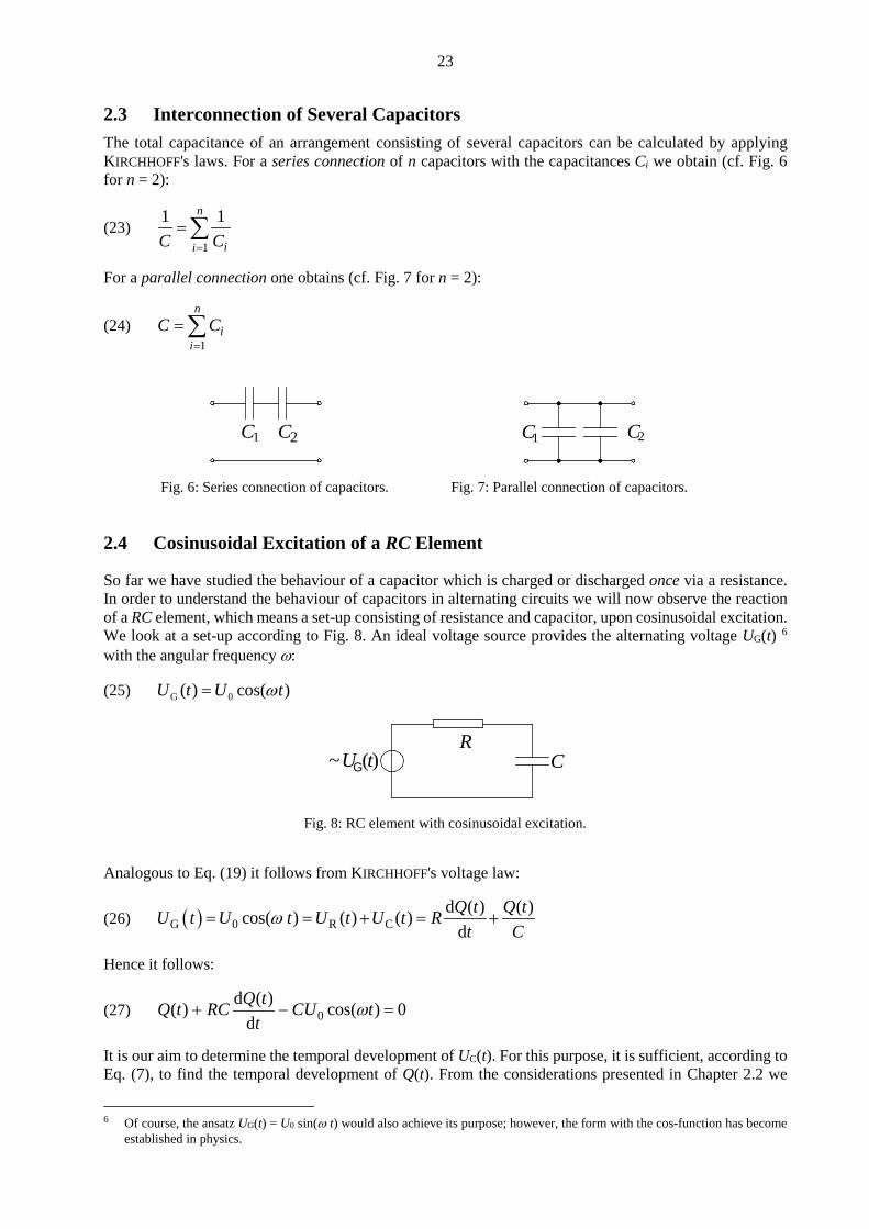
Fig. 6: Series connection of capacitors. Fig. 7: Parallel connection of capacitors.

2.4 Cosinusoidal Excitation of a RC Element

So far we have studied the behaviour of a capacitor which is charged or discharged once via a resistance. In order to understand the behaviour of capacitors in alternating circuits we will now observe the reaction of a RC element, which means a set-up consisting of resistance and capacitor, upon cosinusoidal excitation. We look at a set-up according to Fig. 8. An ideal voltage source provides the alternating voltage UG(t) 6 with the angular frequency ω:

(25) G 0( ) cos( )U t U tω=

Fig. 8: RC element with cosinusoidal excitation. Analogous to Eq. (19) it follows from KIRCHHOFF's voltage law:

(26) ( )G 0 R Cd ( ) ( )cos( ) ( ) ( )

dQ t Q tU t U t U t U t R

t Cω= = + = +

Hence it follows:

(27) 0d ( )( ) cos( ) 0

dQ tQ t RC CU t

tω+ − =

It is our aim to determine the temporal development of UC(t). For this purpose, it is sufficient, according to Eq. (7), to find the temporal development of Q(t). From the considerations presented in Chapter 2.2 we

6 Of course, the ansatz UG(t) = U0 sin(ω t) would also achieve its purpose; however, the form with the cos-function has become

established in physics.

C1 2C 1C C2

~ U (t)G

RC

24

know that the capacitor cannot be charged or discharged infinitely rapidly. This means that the course of charging Q(t) cannot follow the voltage UG(t) instantaneously, but rather with a certain temporal delay. Therefore, we expect a phase shift ϕ of Q(t) compared to UG(t). Thus, we try to solve the differential equation (27) by setting: (28) Q t Q t( ) cos( )= +0 ω ϕ By inserting Eq. (28) into Eq. (27) we now have to determine the unknown quantities Q0 and ϕ. Following some calculations (which are most easily done using complex quantities, see appendix in Chap. 4) we obtain for the maximum charge Q0 of the capacitor:

(29) ( )

00 2 1

CUQRCω

=+

and for the phase shift ϕ between Q(t) or UC(t) and UG(t): (30) arctan( )RCϕ ω= − and (31) tan RCϕ ω= − , respectively. From Eq. (30) we learn that ϕ is always negative. The charge Q(t) always lags behind the voltage UG(t). For the limit ω → 0 we obtain ϕ ≈ 0° and for the limit ω → ∞ it follows: ϕ = -90°. With the relationship:

(32) 2 2

1 1costan 1 ( ) 1RC

ϕϕ ω

= =+ +

we obtain by inserting Eq. (32) into Eq. (29):

(33) 0 0 cosQ CU ϕ= Comparing Eqs. (1) and (33) we learn that the maximum charge of the capacitor is lower by a factor of cos ϕ under a cosinusoidal excitation than under a direct voltage of magnitude U0. For the limit ω →0 we obtain Q0 ≈ CU0 and for the limit ω → ∞ it follows that Q0 = 0. Question 4: - How can these extreme cases be illustrated? We will now calculate the temporal course of the current I(t) through the loop according to Fig. 8. We have:

(34) d ( )( )

dQ tI t

t=

Inserting Eq. (28) into (34) and performing the differentiation yields:

(35) ( ) ( )0 0 0( ) sin cos cos2

I t Q t Q t I tπω ω ϕ ω ω ϕ ω θ = − + = + + = +

with the current amplitude I0:

25

(36) 00 0

22

1( )

UI QR

C

ω

ω

= =+

and the phase shift θ between the current I(t) and the voltage UG(t):

(37) θ ϕ π= +

2

Using the relationship tan(ϕ + π/2) = -1/tanϕ, we obtain from Eqs. (37) and (31):

(38) 1tanRC

θω

=

Eq. (38) shows that in the case ω →0 the current I(t) precedes the voltage UG(t) by 90° (θ = π/2). In the case ω →∞, however, current and voltage are in phase (θ ≈ 0°). With increasing frequency the phase shift between current and voltage decreases from 90° to 0°.

2.5 Impedance The impedance (or apparent resistance) is an important parameter for the description of electrical circuits. It will be treated in more detail in the experimental physics lecture of the second semester. For this reason, we will restrict ourselves here to a few remarks on impedance. The impedance Z is defined as the total resistance7 an electrical circuit poses to an alternating voltage of angular frequency ω. It follows that Z = Z(ω). The unit of impedance is Ohm:

[ ]Z = Ω An impedance in an AC circuit will, in general, influence the amplitude and the phase of the current in a circuit. Thus it is practical to represent it as a complex quantity:

(39) ( ) ( )Re ImZ Z i Z= + Fig. 9 shows Z as a pointer in the plane of complex numbers. The real part of Z is the (ohmic) resistance R of a circuit:

(40) ( )ReR Z= The imaginary part of Z is called reactance X8:

(41) ( )ImX Z= Thus, we can write for Z (according to equation (39)):

(42) Z R i X= + The magnitude of Z (i.e. the length of the arrow in Fig. 9) is given by:

(43) 2 2Z R X= +

7 In general, the total resistance is not a pure ohmic resistance! 8 In an AC circuit with capacitor C and coil L, the reactance X is composed of an inductive component caused by L, and a

capacitive component caused by C. More about this in the second semester.

26

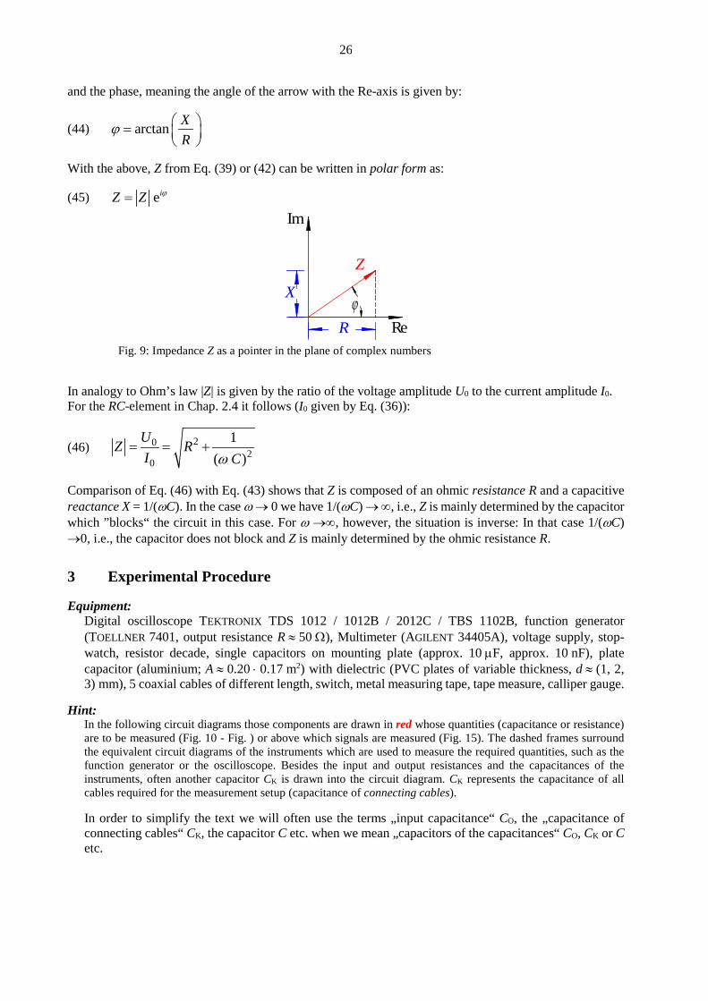
and the phase, meaning the angle of the arrow with the Re-axis is given by:

(44) arctan XR

ϕ =

With the above, Z from Eq. (39) or (42) can be written in polar form as:

(45) eiZ Z ϕ=

Fig. 9: Impedance Z as a pointer in the plane of complex numbers

In analogy to Ohm’s law |Z| is given by the ratio of the voltage amplitude U0 to the current amplitude I0. For the RC-element in Chap. 2.4 it follows (I0 given by Eq. (36)):

(46) 202

0

1( )

UZ RI Cω

= = +

Comparison of Eq. (46) with Eq. (43) shows that Z is composed of an ohmic resistance R and a capacitive reactance X = 1/(ωC). In the case ω → 0 we have 1/(ωC) → ∞, i.e., Z is mainly determined by the capacitor which ”blocks“ the circuit in this case. For ω →∞, however, the situation is inverse: In that case 1/(ωC) →0, i.e., the capacitor does not block and Z is mainly determined by the ohmic resistance R.

3 Experimental Procedure

Equipment: Digital oscilloscope TEKTRONIX TDS 1012 / 1012B / 2012C / TBS 1102B, function generator (TOELLNER 7401, output resistance R ≈ 50 Ω), Multimeter (AGILENT 34405A), voltage supply, stop-watch, resistor decade, single capacitors on mounting plate (approx. 10 µF, approx. 10 nF), plate capacitor (aluminium; A ≈ 0.20 ⋅ 0.17 m2) with dielectric (PVC plates of variable thickness, d ≈ (1, 2, 3) mm), 5 coaxial cables of different length, switch, metal measuring tape, tape measure, calliper gauge.

Hint:

In the following circuit diagrams those components are drawn in red whose quantities (capacitance or resistance) are to be measured (Fig. 10 - Fig. ) or above which signals are measured (Fig. 15). The dashed frames surround the equivalent circuit diagrams of the instruments which are used to measure the required quantities, such as the function generator or the oscilloscope. Besides the input and output resistances and the capacitances of the instruments, often another capacitor CK is drawn into the circuit diagram. CK represents the capacitance of all cables required for the measurement setup (capacitance of connecting cables). In order to simplify the text we will often use the terms „input capacitance“ CO, the „capacitance of connecting cables“ CK, the capacitor C etc. when we mean „capacitors of the capacitances“ CO, CK or C etc.

Im

Re

Z

ϕR

X

27

3.1 Determining the Input Resistance of an Oscilloscope from the Discharge Curve of a Capacitor

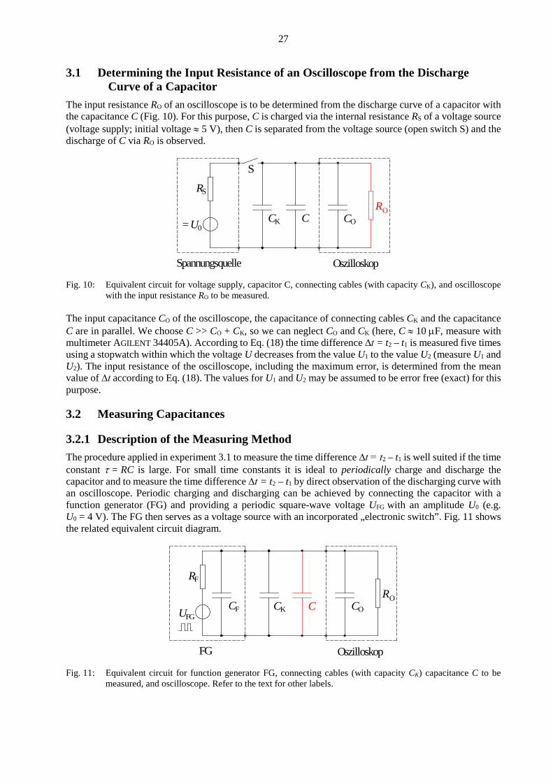
The input resistance RO of an oscilloscope is to be determined from the discharge curve of a capacitor with the capacitance C (Fig. 10). For this purpose, C is charged via the internal resistance RS of a voltage source (voltage supply; initial voltage ≈ 5 V), then C is separated from the voltage source (open switch S) and the discharge of C via RO is observed.

Fig. 10: Equivalent circuit for voltage supply, capacitor C, connecting cables (with capacity CK), and oscilloscope with the input resistance RO to be measured.

The input capacitance CO of the oscilloscope, the capacitance of connecting cables CK and the capacitance C are in parallel. We choose C >> CO + CK, so we can neglect CO and CK (here, C ≈ 10 µF, measure with multimeter AGILENT 34405A). According to Eq. (18) the time difference ∆t = t2 – t1 is measured five times using a stopwatch within which the voltage U decreases from the value U1 to the value U2 (measure U1 and U2). The input resistance of the oscilloscope, including the maximum error, is determined from the mean value of ∆t according to Eq. (18). The values for U1 and U2 may be assumed to be error free (exact) for this purpose.

3.2 Measuring Capacitances

3.2.1 Description of the Measuring Method The procedure applied in experiment 3.1 to measure the time difference ∆t = t2 – t1 is well suited if the time constant τ = RC is large. For small time constants it is ideal to periodically charge and discharge the capacitor and to measure the time difference ∆t = t2 – t1 by direct observation of the discharging curve with an oscilloscope. Periodic charging and discharging can be achieved by connecting the capacitor with a function generator (FG) and providing a periodic square-wave voltage UFG

with an amplitude U0 (e.g. U0 = 4 V). The FG then serves as a voltage source with an incorporated „electronic switch”. Fig. 11 shows the related equivalent circuit diagram.

Fig. 11: Equivalent circuit for function generator FG, connecting cables (with capacity CK) capacitance C to be

measured, and oscilloscope. Refer to the text for other labels.

C

Spannungsquelle

K

SR

S

CR

C

Oszilloskop

OO

= U0

C

FG

K

FR

CR

C

Oszilloskop

OO

UFGCF

28

A comparison with Fig. 10 shows two differences: a) Besides the capacitance of the connecting cables (CK), the input capacitance of the oscilloscope

(CO) and the capacitance C to be measured the “output capacitance”9 CF of the FG has to be taken into account. These three capacities together form the total capacitance CA of the measuring set-up:

(47) A O K FC C C C= + + b) The FG as an „electronic switch“ does not separate the voltage source with resistance RF (≈ 50 Ω)

from the circuit (like the switch S in Fig. 10), but only causes a periodic charge reversal of the capacities CA and C.10 Due to RF << RO the charge reversal is performed via RF. Therefore RF deter-mines the time constant τ of the RC element together with CA and C. In this case, Eq. (18) therefore reads:

(48) 2 1A

1

2lnF

t tC CUR U

−+ =

Eq. (48) provides the possibility to determine an unknown capacitance C by measuring U1, U2 and ∆t = t2 – t1, provided that RF and CA are known. For the function generators used in the laboratory course RF ≈ 50 Ω. This results in a small value of the time constant τ of the capacitor discharge, leading to a small (and hence difficult to measure) time difference ∆t = t2 - t1. For this reason, an external resistance RD ≈ 1 kΩ from the resistance decade is placed in series with RF in a set-up according to Fig. 12 in order to achieve a total resistance of

(49) G F DR R R= + thus increasing the time difference ∆t. Eq. (48) then becomes:

(50) 2 1A

1G

2ln

t tC CUR U

−+ =

Fig. 12: Circuit from Fig. 11 with added resistor RD.

9 A real square-wave signal from a FG never has edges with slope ∞. Rather, e.g. the falling edge resembles the discharging

curve of a capacitor with capacitance CF. This quantity is described as output capacitance according to an equivalent circuit here.

10 It is of no importance to the measurement, whether the capacitor is charged and then discharged or periodically commutated, as in this case. This does not influence the time response.

C

FG

K

FR

CR

C

Oszilloskop

OO

UFGCF

DR

29

Fig. 13: Picture of the circuit from Fig. showing the function generator on the left, the oscilloscope on the right,

and the resistance decade with resistor RD in the centre. RD is located between the two black terminals of the resistance decade. The yellow terminal is a support contact without an electrical connection to RD. A BNC-T connector is inserted in the cable connecting the resistance decade and the oscilloscope in order to connect the capacitor for which the capacitance C is to be determined.

From this follows, that the capacitance C is given by:

(51) 2 1A

1G

2ln

t tC CUR U

−= −

3.2.2 Preliminary Measurements In order to determine an unknown capacitance C from Eq. (51), the value of the total capacitance CA of the circuit needs to know in addition to the resistance RG. CA is determined by setting up the circuit according to Fig. 12 with C = 0 (i.e. without the capacitance C to be measured). A BNC-T piece is included in the circuit (Fig. 13) to connect the capacitance C which is to be determined for each subsequent measurement. CA can now be determined using Eq. (50). For this purpose, the discharge curve of CA is displayed on the oscilloscope and the time difference ∆t = t2 – t1 associated with the voltage drop from U1 to U2 is measured. For measuring these quantities, the digital oscilloscope can be operated in the mode → Acquisition → Mean value. In this operation mode, the influence of signal noise is minimized. U1 and U2 may be taken as exact values for calculating the maximum error of CA. For RG, a maximum error of 0.01 × RG , in accordance with the accuracy of the resistance decade, may be used. Once these preparations have been made, unknown capacitances C added to the circuit can be measured. Hint:

Eqs. (18) and (51) hold for the discharge of a charged capacitor from an initial voltage U0 to 0 V. The voltage levels U1 and U2 are positive at all times t. If, however, a rectangular voltage with amplitude U0 is applied to the capacitor, it follows that the maximum voltage is + U0 and the minimum voltage is - U0 (Fig. 14, left ordinate). Hence, the resulting reloading curve may include negative voltage values. In this case, Eqs. (18) and (51) cannot be applied, since the logarithm function is only defined for arguments having a positive value. This problem can be solved by recognising that the temporal evolution of a reloading curve from the voltage + U0 to - U0 has the same shape as the discharge curve of a capacitor having an initial voltage of 2 U0 and a minimum voltage of 0 V (Fig. 14, right ordinate). Thus, adding the amplitude U0 to all voltage values recorded from the oscilloscope ensures that U1 and U2 are always positive, and hence Eqs. (18) and (51) can be used.

This method requires, that the rectangular voltage signal does not have any DC component (DC-Offset knob on the FG must be set to OFF) and that its amplitude U0 is known. It follows that U0 must be measured once. To facilitate reading the voltage levels off the oscilloscope, it is recommended to place the signal symmetrically about the centre (horizontal) line of the scale (“0” in Fig. 14, left ordinate). In this case, U1 and U2 can be determined simply by reading the scale marks on the oscilloscope’s screen and ∆t can be determined by using the time cursors.

30

Fig. 14: Charge reversal curve of the capacitor upon applying a rectangular voltage of amplitude U0 without DC-

offset (left ordinate). The same temporal course results for a rectangular voltage with amplitude U0 and DC-offset U0 (right ordinate, blue). The horizontal lines indicate the scale ticks of the oscilloscope.

3.2.3 Determination of the Capacitance of Coaxial Cables In this part of the experiment the capacitance C of coaxial cables added to the existing (coaxial-) cables (having a total capacitance CK), is to be measured. The simplest method to achieve this is to connect the extraneous cables to the BNC-T connector (Fig. 13). C is thus connected parallel to CA. Five coaxial cables of different lengths L ≥ 1 m (measure the lengths!) are connected in turn to the BNC-T-piece. For each cable, the quantities U1, U2, t1 and t2 are measured and the capacitance C is calculated according to Eq. (51). Stating the errors for the individual values of C may be omitted. As a result the mean value of the capacitance of the coaxial cable per meter including the standard deviation of the mean is to be stated and to be compared with the index value for coaxial cables of the type RG 58 C/U (101 pF/m).

3.2.4 Determining the Relative Permittivity of PVC Following the method described in Chapter 3.2.2 the capacitance of a plate capacitor with the dielectric PVC between its plates is to be determined. The objective is to determine the relative permittivity εr of PVC from a series of capacitance measurements with varying thickness d of the dielectric. The plate capacitor consists of two equal aluminium plates of the area A with a PVC plate of equal size and thickness d between them. The capacitor is connected between function generator and oscilloscope in addition and in parallel to the existing connecting cables. It is connected to the BNC-T-piece by a coaxial cable having laboratory plugs on the other end11. One of the aluminium plates is put on the laboratory bench and connected to the „negative pole” of the function generator (outer contact of the BNC-connector). The PVC plate is put on this plate and the second aluminium plate is put on top of it and connected to the other pole of the function generator. Measurements are done for PVC plate sizes of d ≈ (3, 4, 5, 6) mm (measure d with a calliper gauge and A with a metal measuring tape). C is determined for each size (Eq. (51)). For further analysis, C is plotted over 1/d. εr can be determined (Eq. (6)) from the slope of the regression line and can be compared with the literature value (Eq. (6)).12

3.3 Phase Shift Between Current and Voltage in an RC Element Using a set-up according to Fig. 15 the phase shift θ between the cosinusoidal output voltage UFG of the function generator and the charge and discharge current I of the capacitor with dependence on the angular frequency ω is to be measured. We can neglect the internal resistances as well as input and output capaci-tances of the function generator and the oscilloscope for this experiment. 11 This additional cable increases the total capacity CK of the connecting cables in the experimental setup. It is thus necessary to

(re-)measure the total capacity CA of the measuring apparatus prior to connecting the parallel plate capacitor. 12 Literature value according to /3/: εr = 3.1 … 3.5 (without stating frequency).

U1

U2

U

t1 t2 t-U0

+U0

0

2U0

U0

0

31

The output voltage UFG of the function generator can be measured directly using the oscilloscope (sym-bolized by the “voltmeter” V1 in Fig. 15). The current I is measured via a small detour: I causes a voltage drop, UR = R I at R, that is in phase with I and can also be measured with the oscilloscope (V2). The measurement of θ is carried out for an RC element with R ≈ 1 kΩ and C ≈ 10 nF (measure both values with multimeter AGILENT 34405A) at frequencies of f = (1, 5, 10, 20, 30, 40, 50, 100) kHz. The amplitude of UFG shall amount to approx. 5 V at f = 10 kHz. θ is plotted vs. ω with maximum error for θ. Into the same diagram the theoretical expected values for θ are plotted too and are compared with the measured data.

Fig. 15: Set-up for measuring the phase shift between UG(t) and I(t) in a RC element.

Practical hints: - When carrying out the experiment it should be considered that the reactance X = 1/(ωC) of the capacity

is a function of ω so that the voltage amplitudes also vary with ω . - The phase shift θ can best be determined by measuring the time difference ∆t of the passages through

zero by both voltages UG(t) and UR(t) (compare with the experiment “Oscilloscope...”). - Consider at the connecting of the cables for the measurement of UG(t) and UR(t) that the outer contacts

of the BNC sockets of the oscilloscope are on the same potential! Consequently this also applies to the outer contacts of the BNC plugs at the coaxial cables!

Question 5: - How large is the phase shift between the voltage at the capacitor (UC) and the current I? How can the

phase shift be measured?

4 Appendix

Calculating with complex quantities, Eqs. (29) and (30) are easy to derive. In a complex form the formulas in Eqs. (25) and (28), respectively, can be written as:

(52) G 0( ) ei tU t U ω=

(53) ( ) ( )0 ei tQ t Q ω ϕ+=

Inserting both equations into Eq. (26) and performing the differentiation we obtain after division by ei tω :

(54) 0 0 01e ei iU i RQ QC

ϕ ϕω= +

Hence it follows:

(55) 00 e 1

i UQi R

C

ϕ

ω=

+

C

R VV1

2

FG

FR

~ UFG

32

The left side of Eq. (55) is one common way to represent a complex number (polar notation) z of modulus |z| and the phase angle (argument) ϕ:

(56) 0 0: e here: e ,iz z z Q z Qϕ ϕ−= = = The modulus of z is given by

(57) z z z∗= z* being the complex conjugated to z which is obtained by changing the sign of the imaginary unit i (i → -i and -i → i). For the modulus Q0 we thus obtain:

(58) ( ) ( )

20 0 0 0

0 222

1 1 1 1

U U U U CQRCi R i R R

C C Cωω ω ω

= = =++ − +

This is the result given in Eq. (29) . We use a second common method to represent complex numbers to calculate the phase angle, namely

(59) ( ) ( )Re Im :z z i z iα β= + = + where α is the real part (Re) and β the imaginary part (Im) of z. From these quantities the phase angle ϕ can be calculated as

(60) π 0 0

arctanπ 0 0

α ββϕα βα

+ ⇔ < ∧ ≥ = − ⇔ < ∧ <

In order to apply Eq. (60), we have to convert Eq. (55) into the form of Eq. (59), that is we must separate the real and the imaginary part from each other. For this purpose we have to eliminate i from the denomi-nator, for which the fraction is appropriately extended. Eq. (55) then becomes:

(61)

000

02 2 2 2

2 2

1

e :1 11 1i

UU i RU RC CQ i i

R Ri R i RC CC C

ϕω

ωα β

ω ωω ω

− = = − = +

+ ++ −

From Eq. (61) we can read off α and β :

(62) 0

2 22

1

UC

RC

αω

=+

0

2 22

1

UC

RC

αω

=+

Attention must be paid to the fact that there is a positive sign in the definition equation (59). Thus, the negative sign of i in Eq. (61) belongs to the imaginary part β! By inserting Eq. (62) into Eq. (60) we obtain:

(63) ( )arctan arctan RCβϕ ωα

= = −

This is the result given in Eq. (30).

33

Carl von Ossietzky University Oldenburg – Faculty V - Institute of Physics Module Introductory laboratory course physics – Part I

Sensors for Force, Pressure, Distance, Angle, and Light Intensity Keywords:

Sensor, linearity, response time, measuring range, resolution, noise, strain gauge, piezoresistive effect, triangulation, HALL-effect, semiconductor, pn-junction.

Measuring program: Calibration of a force sensor and a pressure sensor, distance measurement with a laser distance sensor, measurement of the transmission ratio with an angle sensor, linearity of the output signal of a photo diode, measurement of the power of laser light, measurement of the velocity of a finger movement.

References: /1/ NIEBUHR, J.; LINDNER, G.: „Physikalische Messtechnik mit Sensoren“, Oldenbourg-Industrieverlag, München /2/ SCHANZ, G. W.: „Sensoren“, Hüthig-Verlag, Heidelberg /3/ HAUS, J.: „Optical Sensors“, Wiley-VCH, Weinheim

1 Introduction

A sensor is a device for the quantitative acquisition of a physical or a chemical quantity. In most cases, the value w of the quantity is converted into an electrical voltage U or an electrical current I. By performing a calibration, the calibration function U(w) (or I(w) resp.) is obtained; it allows determining the value of the quantity from the measured value of the voltage or current. For calibrating a force sensor, for example, the sensor is submitted to varying, yet known forces Fi and the corresponding voltage Ui is measured in each case. Subsequently, Ui is plotted over Fi and a calibration curve is obtained by performing a fit on the measured values. Important characteristic parameters of sensors are: Linearity: Often a linear relationship exists between the actual value of the quantity w and the output

signal of the sensor, e.g. the voltage U. In this case:

0U k w U= + where k is the calibration factor and U0 the output voltage of the sensor for the case w = 0. In this case, the calibration curve is a line, the sensor operates in a linear manner. If U0 = 0, a proportionality exists between U and w. This is the ideal case for a sensor.

Response time: The response time is the time interval required for a change in the quantity w to cause a corresponding change in the output signal.

Measuring range: The measuring range defines the range of values of the quantity w, which causes a change of the output signal which can be described by the calibration function, within a defined margin of error.

Resolution: The resolution is the smallest change of the quantity w, which leads to a distinctively measurable change of the output signal.

Noise: The inherent, random fluctuations in the output signal of a sensor are called noise. One of the main sources for the noise of many sensors is the electronics employed for the creation of the output signal.

The use of sensors in measurement technology, and industrial production has become widespread since it became possible to produce sensors in compact miniaturized packages, or even integrate them directly into IC’s1. In this experiment, sensors for force, pressure in gases, distance, angle, and light intensity will be treated. 1 IC: Integrated Circuit. An integrated electrical circuit inside a ceramic or plastic casing.

34

2 Theory

2.1 Bending Rod as a Force Sensor The force sensors used in the introductory laboratory course transform a mechanical force of magnitude F into a voltage signal U that varies linearly with F.

Fig. 1: Left: Principle of force measurement using a bending rod (green) fixated on the left by a block (gray). The

gravitational force F = G of a suspended weight (blue) causes a deformation of the staff which is measured by the strain gauge (SG, yellow). The mechanical limits (red) prevent overstraining the rod by excessive forces.

Right: View into the casing of a force sensor used in this laboratory course. The strain gauges glued to the rod are very thin and barely visible. The cables are the connections of the SG. They run to the connecting terminal on the top left to which the measuring amplifier is connected.

Fig. 2: Half bridge with two SGs of the same type and two equal resistors R. One SG is elongated while the other one is compressed. Ub is the supply voltage of the bridge, U the output voltage which is amplified by a measuring amplifier.

A bending rod (cf. Fig. 1) is used as the sensor. The staff is fixed at one end and elastically deformed by the force F, HOOKE‘s law applies2. The rod is elongated on the top side while it is compressed on the bottom side. Elongation and compression are proportional to F = |F|. The deformations are translated into changes in electrical resistance proportional to F by strain gauges (SG). The SGs are connected to form a half-bridge (cf. Fig. 2)3. The supply voltage Ub is connected to one bridge diagonal, while the output voltage U is measured at the other diagonal. Since this voltage is very small (in the mV range), it is amplified by a measuring amplifier which also provides the supply voltage Ub. The output voltage of the measuring amplifier, UM, changes linearly with F.

2.2 Pressure Sensor on the Basis of the Piezoresistive Effect A sensor of the type SENSORTECHNICS HCLA12X5DB is available for the measurement of pressure changes in gases. It is a semiconductor sensor and its operation is based on the piezoresistive effect, which is the change in electrical resistance of a material (in this case p-silicone, p-Si; cf. Chap. 2.5.1 for labeling)

2 ROBERT HOOKE (1635 – 1703) 3 Compare experiment „Measurement of Ohmic Resistances…“

FDMS

b=U

R

R

+

-

DMS

DMS

U

35

under the influence of mechanical tension. Fig. 3 (left) depicts the schematic setup for such a sensor. A silicone membrane with a width of several micrometers divides a gas-tight chamber in the centre, separating it into two gas-tight parts. The upper half of the chamber is connected (using a tube) to a volume of gas at pressure p1 while the other half is connected to a volume of gas having pressure p2. A pressure difference ∆p = p2 – p1 causes the membrane to bulge towards the chamber with lower pressure. The border of the membrane is fitted with piezoresistive sensors that experience forces as a result of the deformation of the membrane. The tension causes an elongation, and hence a change of resistance in the material4 which is converted to a voltage signal by using a bridge circuit integrated in the sensor. The signal is amplified by an integrated circuit, which is also already part of the sensor. At the output of the pressure sensor, a voltage U is thus available which changes linearly with the pressure difference ∆p.5

Fig. 3: Left: Schematic representation of a piezoresistive pressure sensor for measuring a pressure difference

∆p = p2 – p1. Right: View into the casing of a pressure sensor used in this laboratory course. The sensor integrated in an

IC can be seen on the right (inside) on a small circuit board. The tube connectors can be seen on the outside of the casing on the right (p1 = p-, p2 = p+).

2.3 Distance Sensor on the Basis of Triangulation A laser distance sensor is used for distance measurements (type BAUMER OADM 12U6460/S35). The sensor uses the principle of triangulation (cf. Fig. 4 left). A thin, collimated beam of laser light from a laser diode is incident on the surface of an object O. The distance of the reflective surface to a plane of reference E within the sensor is to be measured. The centre of an objective L is placed at a lateral distance d from the exit of the laser beam. This objective focuses the light reflected at point C of the object onto a one dimensional CCD-array6. This results in a point image A at a distance q from the right border of the CCD-array. The distance q varies with the distance s between E and O. For the triangle ABC (hence the name triangulation) we have:

(1) tan d qs

α +=

x In addition, using the distance p between the central plane of the lens and the front side of the CCD-array (plane E) we get:

(2) tan qp

α =

4 The effect is comparable to the change of resistance of a metallic SG under elongation. The change in resistance associated

with a certain elongation of a piezoresistive material is, however, significantly larger than in the case of a metallic SG. For metals, k = 2 – 4, for Si k ≈ 100 (cf. Experiment “Measuring ohmic resistances…”).

5 The electrical connection (bond) between the integrated circuit and the piezoresistive elements is established by thin bonding filaments connected to bonding pads.

6 CCD: Charge Coupled Device. A one dimensional CCD-array consists of a number of e.g. 128 or 512 (or more) small photodetectors (pixels) with an individual width of a few micrometers arranged in a straight line.

Anschlusskontakt("Bonding Pad")

PiezoresistivesSi-Element

Si-Membran

p

p2

1

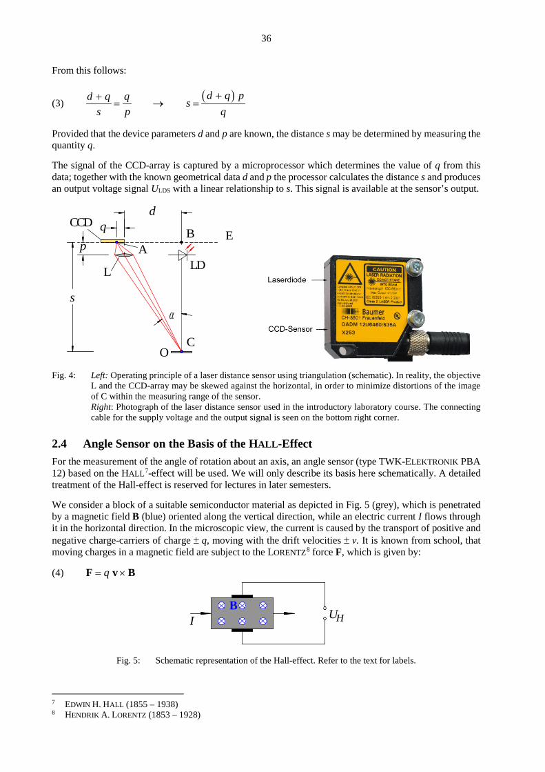
36

From this follows:

(3) ( )d q pd q q s

s p q++

= → =

Provided that the device parameters d and p are known, the distance s may be determined by measuring the quantity q. The signal of the CCD-array is captured by a microprocessor which determines the value of q from this data; together with the known geometrical data d and p the processor calculates the distance s and produces an output voltage signal ULDS with a linear relationship to s. This signal is available at the sensor’s output.

Fig. 4: Left: Operating principle of a laser distance sensor using triangulation (schematic). In reality, the objective

L and the CCD-array may be skewed against the horizontal, in order to minimize distortions of the image of C within the measuring range of the sensor.

Right: Photograph of the laser distance sensor used in the introductory laboratory course. The connecting cable for the supply voltage and the output signal is seen on the bottom right corner.

2.4 Angle Sensor on the Basis of the HALL-Effect For the measurement of the angle of rotation about an axis, an angle sensor (type TWK-ELEKTRONIK PBA 12) based on the HALL7-effect will be used. We will only describe its basis here schematically. A detailed treatment of the Hall-effect is reserved for lectures in later semesters. We consider a block of a suitable semiconductor material as depicted in Fig. 5 (grey), which is penetrated by a magnetic field B (blue) oriented along the vertical direction, while an electric current I flows through it in the horizontal direction. In the microscopic view, the current is caused by the transport of positive and negative charge-carriers of charge ± q, moving with the drift velocities ± v. It is known from school, that moving charges in a magnetic field are subject to the LORENTZ8 force F, which is given by: (4) q= ×F v B

Fig. 5: Schematic representation of the Hall-effect. Refer to the text for labels.

7 EDWIN H. HALL (1855 – 1938) 8 HENDRIK A. LORENTZ (1853 – 1928)

OC

d

s

q

Ap

α

BCCD

L LD

E

IB

UH

37

In a setup according to Fig. 5, the LORENTZ force causes positive charge carriers to move to the top and negative charge carriers to the bottom. This results in a Hall-voltage UH forming between the contacts (black) given by:

(5) ~HU B It is evident from Eq. (4), that the magnitude of the force F depends on the angle α between v and B. It holds:

(6) sinF q v B q v Bα ⊥= = where Β⊥ is the component of B standing perpendicular on v. A change of the force F is accompanied by a proportional change of the Hall-voltage. It holds:

(7) ~HU B⊥ Eq. (7) forms the basis for the angle sensor used in the experiment, its operating principle is depicted schematically in Fig. 6.

Fig. 6: Schematic of the angle sensor used in the experiment. Refer to the text for labels. A small permanent magnet is mounted on the axis whose angular position α is to be measured. Upon rotation of the axis, the magnetic field B, caused by the magnet, is rotated by the same angle. This field penetrates two9 Hall-sensors H1 and H2. Depending on the orientation of B, H1 and H2 provide two differ-ent Hall-voltages, which are transformed by an ASIC10 to create the output voltage UW of the angle sensor, which is proportional to the angleα.

2.5 Photodetectors Photodetectors are used for the detection of light. Measurable quantities are the light power PL with the unit W (Watt) or the light intensity IL with the unit W/m2. We will restrict ourselves from the multitude of different photodetectors to the photodiode. It converts the quantities PL or IL into an electric current I which changes in a linear fashion with PL, or IL respectively. A current to voltage converter may be used to convert the current I to a proportional voltage U, if the need arises. Knowledge of solid state physics and semiconductor physics, which will be acquired in later semesters, is required for a detailed understanding of how a photodiode works. For this reason, we will restrict ourselves to a short description of the basics of its construction and operating principle.

2.5.1 Si-Semiconductor and pn Junction The majority of photodiodes are manufactured from crystalline silicone (Si), which is a semiconductor. Every four valued atom in pure (intrinsic) Si is connected to four other Si atoms by covalent bonds (cf. Fig. 7). The four electrons of the outer shell are thus spatially fixated.

9 Two Hall-sensors are required in order to determine the sign of a rotation unambiguously. 10 ASIC: Application Specific Integrated Circuit.

ASICH 1H 2

NS U

α

38

Fig. 7: Crystal structure of pure Si. The blue circles represent (schematically) the electrons making up the covalent bonds.

Doping of pure Si with five-valued atoms (donors) creates n-silicon (Fig. 8 left), which is a n-semiconduc-tor11. Only four electrons are needed for the covalent bonds of the donor atom with the four neighboring Si atoms. The bond between the fifth electron (negative n-charge carrier) and the core of the donor atom is rather weak. This electron can thus move though the material nearly unobstructed. By doping pure silicon with three-values atoms (acceptors) p-silicon can be created (Fig. 8 right) which is a p-semiconductor. One electron is missing in the covalent bond of the acceptor atom with the four Si-neighbors. This leaves a hole, which behaves like a positive charge carrier (p-charge carrier). This hole is able to capture an electron from its surrounding. The captured electron leaves a new hole, which can again capture an electron from its surrounding. The hole may thus move through the material, it is mobile.

Fig. 8: Left: Crystal structure of n-Si where several four-valued Si-atoms are replaced by five-valued atoms, in this case arsenic (As). The fifth valence electron of the As atom is a mobile n-charge carrier.

Right: Crystal Structure of p-Si where several four-valued Si atoms are replaced by three-valued atoms, in this case boron (B). The missing valence electron of the B atom, called a hole, is a mobile p-charge carrier.

When a p- and a n-semiconductor are brought into contact, a pn junction is formed (cf. Fig. 9). The concen-trations of p- and n-charge carriers differ greatly in the contact region. This causes holes to diffuse from the p-Si to the n-Si where they recombine with the surplus electrons. Analogously, the surplus electrons from the n-Si diffuse into the p-Si region, recombining with the surplus holes. This causes the formation of a region without mobile charge carriers, hence called the depletion zone (S) or barrier layer. The diffusion process leaves positive ionized donors in the n side of the depletion zone and negative ionized acceptors on the p side (cf. Fig. 10). These ions are called space charges, they create an electrical field E (built-in-field) in the depletion zone, also called space charge region in this context.

11 The typical doping concentration in Silicone, which is used for the construction of photodiodes lies within the order of

magnitude 1015 – 1017 impurity atoms / cm3. Pure Si contains approx. 0.5 × 1023 Si-atoms / cm3.

Si Si Si Si

Si Si Si Si

Si Si Si Si

Si Si Si Si

Si Si As Si

Si Si Si Sin

Si Si Si Si

Si Si B Si

Si Si Si Si

p

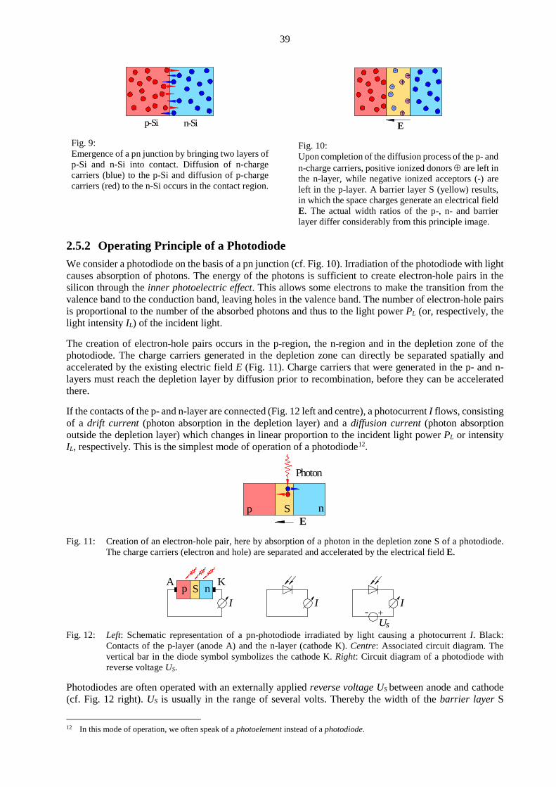
39

Fig. 9: Emergence of a pn junction by bringing two layers of p-Si and n-Si into contact. Diffusion of n-charge carriers (blue) to the p-Si and diffusion of p-charge carriers (red) to the n-Si occurs in the contact region.

Fig. 10: Upon completion of the diffusion process of the p- and n-charge carriers, positive ionized donors ⊕ are left in the n-layer, while negative ionized acceptors (-) are left in the p-layer. A barrier layer S (yellow) results, in which the space charges generate an electrical field E. The actual width ratios of the p-, n- and barrier layer differ considerably from this principle image.

2.5.2 Operating Principle of a Photodiode We consider a photodiode on the basis of a pn junction (cf. Fig. 10). Irradiation of the photodiode with light causes absorption of photons. The energy of the photons is sufficient to create electron-hole pairs in the silicon through the inner photoelectric effect. This allows some electrons to make the transition from the valence band to the conduction band, leaving holes in the valence band. The number of electron-hole pairs is proportional to the number of the absorbed photons and thus to the light power PL (or, respectively, the light intensity IL) of the incident light. The creation of electron-hole pairs occurs in the p-region, the n-region and in the depletion zone of the photodiode. The charge carriers generated in the depletion zone can directly be separated spatially and accelerated by the existing electric field E (Fig. 11). Charge carriers that were generated in the p- and n-layers must reach the depletion layer by diffusion prior to recombination, before they can be accelerated there. If the contacts of the p- and n-layer are connected (Fig. 12 left and centre), a photocurrent I flows, consisting of a drift current (photon absorption in the depletion layer) and a diffusion current (photon absorption outside the depletion layer) which changes in linear proportion to the incident light power PL or intensity IL, respectively. This is the simplest mode of operation of a photodiode12.

Fig. 11: Creation of an electron-hole pair, here by absorption of a photon in the depletion zone S of a photodiode.

The charge carriers (electron and hole) are separated and accelerated by the electrical field E.

Fig. 12: Left: Schematic representation of a pn-photodiode irradiated by light causing a photocurrent I. Black:

Contacts of the p-layer (anode A) and the n-layer (cathode K). Centre: Associated circuit diagram. The vertical bar in the diode symbol symbolizes the cathode K. Right: Circuit diagram of a photodiode with reverse voltage US.

Photodiodes are often operated with an externally applied reverse voltage US between anode and cathode (cf. Fig. 12 right). US is usually in the range of several volts. Thereby the width of the barrier layer S

12 In this mode of operation, we often speak of a photoelement instead of a photodiode.

p-Si n-Si E

++

++

-

--

-

Ep nS

Photon

p nA KS

I+-Us

I I

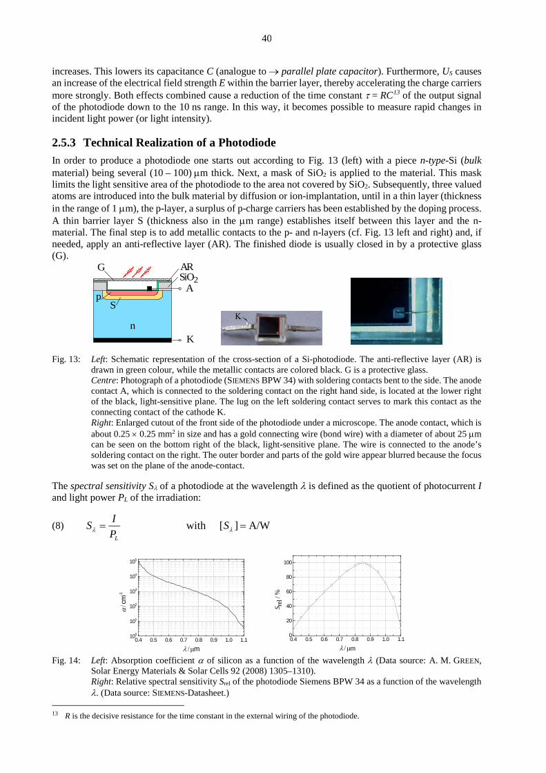
40

increases. This lowers its capacitance C (analogue to → parallel plate capacitor). Furthermore, US causes an increase of the electrical field strength E within the barrier layer, thereby accelerating the charge carriers more strongly. Both effects combined cause a reduction of the time constant τ = RC13 of the output signal of the photodiode down to the 10 ns range. In this way, it becomes possible to measure rapid changes in incident light power (or light intensity).

2.5.3 Technical Realization of a Photodiode In order to produce a photodiode one starts out according to Fig. 13 (left) with a piece n-type-Si (bulk material) being several (10 – 100) µm thick. Next, a mask of SiO2 is applied to the material. This mask limits the light sensitive area of the photodiode to the area not covered by SiO2. Subsequently, three valued atoms are introduced into the bulk material by diffusion or ion-implantation, until in a thin layer (thickness in the range of 1 µm), the p-layer, a surplus of p-charge carriers has been established by the doping process. A thin barrier layer S (thickness also in the µm range) establishes itself between this layer and the n-material. The final step is to add metallic contacts to the p- and n-layers (cf. Fig. 13 left and right) and, if needed, apply an anti-reflective layer (AR). The finished diode is usually closed in by a protective glass (G).

Fig. 13: Left: Schematic representation of the cross-section of a Si-photodiode. The anti-reflective layer (AR) is

drawn in green colour, while the metallic contacts are colored black. G is a protective glass. Centre: Photograph of a photodiode (SIEMENS BPW 34) with soldering contacts bent to the side. The anode

contact A, which is connected to the soldering contact on the right hand side, is located at the lower right of the black, light-sensitive plane. The lug on the left soldering contact serves to mark this contact as the connecting contact of the cathode K.

Right: Enlarged cutout of the front side of the photodiode under a microscope. The anode contact, which is about 0.25 × 0.25 mm2 in size and has a gold connecting wire (bond wire) with a diameter of about 25 µm can be seen on the bottom right of the black, light-sensitive plane. The wire is connected to the anode’s soldering contact on the right. The outer border and parts of the gold wire appear blurred because the focus was set on the plane of the anode-contact.

The spectral sensitivity Sλ of a photodiode at the wavelength λ is defined as the quotient of photocurrent I and light power PL of the irradiation:

(8) with [ ] A/WL

IS SPλ λ= =

Fig. 14: Left: Absorption coefficient α of silicon as a function of the wavelength λ (Data source: A. M. GREEN,

Solar Energy Materials & Solar Cells 92 (2008) 1305–1310). Right: Relative spectral sensitivity Srel of the photodiode Siemens BPW 34 as a function of the wavelength

λ. (Data source: SIEMENS-Datasheet.) 13 R is the decisive resistance for the time constant in the external wiring of the photodiode.

n

pS

SiO2AR

K

A

G

0.4 0.5 0.6 0.7 0.8 0.9 1.0 1.1100

101

102

103

104

105

α / c

m-1

λ / µm0.4 0.5 0.6 0.7 0.8 0.9 1.0 1.10

20

40

60

80

100

S rel

/ %

λ / µm

41

The larger the wavelength λ of the light, by which the photodiode is illuminated, the smaller the absorption coefficient α (Fig. 14 left) and the larger therefore the penetration depth of the photons. Short-wave light is largely absorbed by the protective glass, the anti-reflective layer, or the p-layer, while long-wave light is (mostly) not absorbed before reaching the n-layer. The further away from the depletion layer the photo absorption takes place, the smaller the probability that charge carriers can diffuse to the depletion layer before they recombine. Therefore such photons can only contribute little to the photocurrent. Thus, in total, the photodiode has a λ-dependent spectral sensitivity with an upper limit depending on the band-gap of the semiconductor material (about 1.1 µm for Si). As an example, Fig. 14 (right) shows the relative spectral sensitivity Srel(λ) of the photodiode used in the laboratory course.

3 Experimental Procedure

Attention: Special care must be taken to avoid direct or indirect (by reflection) exposure of the eyes to the laser beam, when conducting experiments involving lasers. Severe retina damage may be caused by the extremely high light intensities! The laser beam must therefore be kept below a height of 1.2 m at all times!

Equipment:

Digital oscilloscope TEKTRONIX TDS 1012 / 1012B / 2012C / TBS 1102B, digital multimeter (AGILENT U1251B and FLUKE 112), 3 power supplies (PHYWE 0 - 15 / 0 - 30) V), force sensor (U-OL) with measuring amplifier (U-OL), set of weights, aluminum-ring, laboratory balance, pressure sensor (SENSORTECHNICS HCLA12X5DB) on base plate with gate valves on mount, ERLENMEYER flask with ground in glass stopper on table, U-pipe-manometer (water filling) with mount and scale, beaker glass on support jack, tubing, laser distance sensor (BAUMER OADM 12U6460/S35), spring with bar and ball on mount, beaker glass with glycerin/water-mixture (190 ml water on 1000 ml glycerine), base plate with angle sensor (TWK-ELEKTRONIK PBA 12) and hand-wheel, photodiode SIEMENS BPW 34, grid-style printed circuit board (8 × 5 cm2) for mounting the photodiode with accessories (50 Ω-resistor, cable, insulating tape, solder), soldering station, wire stripper, clamps, helium-neon laser on triangular rail, polarization filter in THORLABS rotatable mount, U-mount for photodiode, slider.

Note:

Selected characteristics of the sensors used are listed in Tab. 1 of the appendix (Chap. 4).

3.1 Calibration of a Force Sensor The force sensor suspended from a mount is to be calibrated with the aid of a set of weights. For this purpose, the force sensor is connected to the measuring amplifier, which amplifies the bridge voltage U to the voltage UM. The measuring amplifier draws its operating voltage from a power supply, the Damping (Dämpfung) is switched on. The output voltage of the measuring amplifier is measured with a voltmeter for at least 5 weights G in the range of (0 - 100) mN. For the calculation of the masses m of the weights from G = mg, the value of the gravitational acceleration in Oldenburg, g = 9.8133 m/s2 is used, which is as well as m assumed to be an error free quantity14. Subsequently, the measured values of UM are plotted over G and a calibration curve is determined. Since the sensor operates linear, the calibration curve is a line; its parameters are determined by performing a linear regression. Finally, an aluminum ring, which will be used in a later experiment on measuring surface tension, is attached to the force sensor, and the output voltage UM of the measuring amplifier is recorded. With the aid of the calibration curve, the weight G and the mass m of the ring are determined. The maximum error of m follows from the maximum error of UM, the errors of the parameters of the regression line may be neglected. In addition, m is also measured by a laboratory balance (error negligible). Both measured values are compared.

14 Value taken from http://www.ptb.de/cartoweb3/SISproject.php; the error of 2×10-5 m/s2 is neglected.

42

3.2 Calibration of a Pressure Sensor

The pressure sensor is calibrated by applying defined pressure differences ∆p between both of its tube connectors and measuring the resulting output voltage U for each case. The tube connector labeled “-“ is left open, thus remaining in direct contact with the surrounding atmos-phere. The connector labeled “+” is connected to the volume of gas, for which the overpressure ∆p relative to the surrounding is to be measured. Operating the sensor in this mode requires ∆p ≥ 0 in order to obtain a linear response from the sensor (i.e. the pressure at the “+”-connector must be greater than the pressure at the “-“-connector). The maximum allowed pressure difference is ∆p = + 1.25 × 103 Pa, which is converted to a voltage signal of U = U0 + 2 V (U0 = 2.25 V)15 for a supply voltage of + 5 V (power supply). The pressure difference ∆p = 0 Pa creates a voltage of U = U0 + 0 V = U0. For pressure differences in the interval between 0 Pa and 1.25 × 103 Pa, the output voltages lie in the interval U0 ≤ U ≤ U0 + 2 V16.

Fig. 15: Setup for creating pressure differences ∆p > 0 relative to the ambient pressure pL. For details, refer to the

text. The pressure differences required for the calibration of the sensor can be established by using a setup according to Fig. 15. The volume of air in an airtight ERLENMEYER flask E is connected to the pressure sensor D and an U-pipe manometer M by a system of tubes (valve H1 open, valve H2 closed). The pressure p in this volume may be changed by variation of the water level in E. This variation is achieved through raising and lowering a water filled storage vessel (beaker glass) V by using the support jack S. V and E are connected by a hose dipping into the water in both containers. The difference between the pressure p in E and the ambient pressure pL,

(9) Lp p p∆ = − can be measured with the U-pipe manometer. For a difference in height hm in the manometer, it is given by:

(10) m mp h gρ∆ = where ρm is the density of the liquid in the manometer (here: water) and g the gravitational acceleration of earth (g as in Chap. 3.1). A value of 998 kg/m3 may be used for the density ρm of water in the temperature range (20 ± 2) °C and considered to be exact. 15 Note that it would be possible to operate the sensor by keeping the “+”-connector in contact with the surrounding and

connecting a volume of gas at a negative pressure to the “-“-connector. The maximum pressure difference would be ∆p = - 1.25 × 103 Pa, which would be converted to a voltage signal of U = U0 - 2 V.

16 U0 and U vary with the operating voltage (nominal 5 V). An once adjusted voltage may not be changed therefore during the measuring.

Wasser

M

Luft, Druck p

EV

S

hm

Wasser

D

- +pLH

H1

2

43

Question 1: What is the maximum value for the height hm that may be used without exceeding the maximum pressure difference of the sensor?

The output voltage U of the pressure sensor D is measured with a voltmeter for at least 5 different pressure differences (measure the associated heights hm). U is plotted over ∆p (Eq. (10)). Error bars for ∆p are drawn which arise from the maximum errors of the heights hm. After all, the calibration curve is determined and drawn. Since the sensor operates linearly, the calibration curve is a line; its parameters are obtained by using the method of linear regression. Note about the noise:

The electronic noise of the pressure sensor (cf. Tab. 1 in the appendix, Chap. 4) causes fluctuations of the output voltage U, which can be converted into noise of the pressure signal by using the calibration function. This noise is smaller than the pressure fluctuations according to Eq. (10), which are caused by the limited accuracy in reading off the height difference hm. Thus, it may be neglected for the measurements to be performed here.

3.3 Distance Measurement with a Laser Distance Sensor The temporal behavior of a damped harmonic oscillation is to be investigated by employing a laser distance sensor (type BAUMER OADM 12U6460/S35). The angular frequency ω of the oscillation and the damping constant α are sought-after. To measure both quantities we proceed as follows:

Fig. 16: Measuring the course of a damped harmonic oscillation using a laser distance sensor LDS. A ball K is connected to a spring by a rod S according to Fig. 16. The ball is dipped in a glass beaker B containing a glycerin/water mixture providing a damping of the motion. The rod S is released after dis-placing it downwards by several centimeters (adhere to the measuring range of the sensor, cf. Table 1 in the appendix). This causes the ball and bar to execute a damped harmonic oscillation. The displacement from the initial position, x, can be described as a function of the time t by the following equation:

(11) ( ) ( )0 e costx t x tα ω−= where x0 is the initial amplitude (i.e. the initial displacement of the ball), ω the angular frequency of the oscillation, and α the damping constant. Let t = 0 be the time when the bar is released. The displacement x(t) is converted into a voltage signal U(t) by the laser distance sensor. For this purpose, the bar S is fitted with a reflective disk R at which the laser beam of the sensor is aimed. The output voltage of the sensor is given by:

(12) ( ) ( )0 e costDCU t U t Uα ω−= +

K

Feder

B

LDS

R

s

S

44

Here UDC is a direct voltage part depending on the distance between the laser distance sensor LDS and the reflector disc R in the zero position of the sphere.

Fig. 17: Exemplary representation of the output signal of the laser distance sensor according to Eq. (12). In this

example U0 = 2 V and UDC = 5 V. The voltages Ui are measured at the instants ti (here t0 = 0 s, t1 = 0.2 s, t2 = 0.4 s,…).

U(t) is recorded with a digital storage oscilloscope in the SINGLE-SEQ-mode. From the recorded curve the frequency f of the damped oscillation is measured with the time cursors and from that ω is calculated. In order to determine the damping constant α, the amplitudes Ui of the partial oscillations at the instants ti (i = 0, 1, 2, …) are measured with the voltage cursors (Fig. 17). No errors must be indicated for Ui and ti. Ui is plotted vs. ti in a semilogarithmic diagram (Ui on a logarithmic axis). If the natural logarithm is used for scaling the ordinate, then α corresponds to the slope of the regression line through the measured val-ues.17 It is possible to convert the voltage signal U(t) to the quantity x(t) by calibrating the sensor. Question 2:

How would one proceed in order to produce a calibration curve? Since the relationship between U(t) and x(t) is linear, both functions would exhibit the same form. For this reason, calibration and conversion are to be neglected in this case. Question 3:

How could the velocity v(t) and the acceleration a(t) be obtained from the course of x(t)?

3.4 Measurement of a Transmission Ratio with an Angle Sensor A hand-wheel H and an angle sensor W are mounted on a base plate according to Fig. 18. A disk with an O-ring pushing against the rim of the hand-wheel is mounted on the rotational axis of the angle sensor. The output voltage UW of the angle sensor changes in a linear manner between Umin (approx. 0 V) and Umax (approx. 5 V) for a full rotation of its axis. The hand-wheel is turned once from β = 0° to β = 360° (that is by 2π). Thereby W turns by the angle α > 2π. The transmission ratio V = α/2π between the rotation of W and the hand-wheel is determined by measurement of Umin, Umax, Uβ = 0°, Uβ = 360° with a voltmeter and the number n of voltage-jumps from Umax to Umin that occur while β is modified. A statement of the error of V is not required.

17 Take into account the hints to the linear regression in (semi-)logarithmic diagrams in the chapter „Usage of Computers…“

(„Apparent fit“).

0.0 0.2 0.4 0.6 0.8 1.03.0

3.5

4.0

4.5

5.0

5.5

6.0

6.5

7.0

U2

U / V

t / s

U1

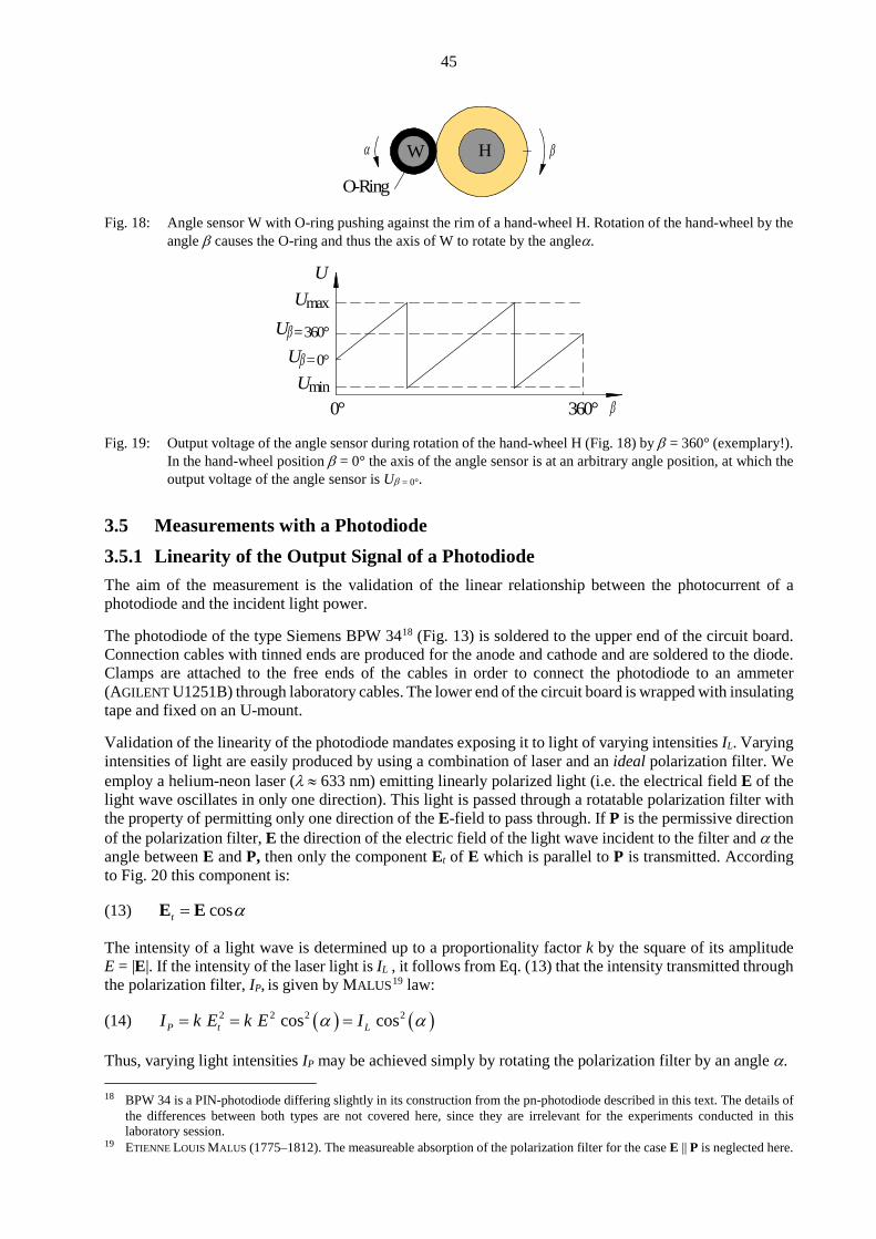
45

Fig. 18: Angle sensor W with O-ring pushing against the rim of a hand-wheel H. Rotation of the hand-wheel by the angle β causes the O-ring and thus the axis of W to rotate by the angleα.

Fig. 19: Output voltage of the angle sensor during rotation of the hand-wheel H (Fig. 18) by β = 360° (exemplary!). In the hand-wheel position β = 0° the axis of the angle sensor is at an arbitrary angle position, at which the output voltage of the angle sensor is Uβ = 0°.

3.5 Measurements with a Photodiode 3.5.1 Linearity of the Output Signal of a Photodiode The aim of the measurement is the validation of the linear relationship between the photocurrent of a photodiode and the incident light power. The photodiode of the type Siemens BPW 3418 (Fig. 13) is soldered to the upper end of the circuit board. Connection cables with tinned ends are produced for the anode and cathode and are soldered to the diode. Clamps are attached to the free ends of the cables in order to connect the photodiode to an ammeter (AGILENT U1251B) through laboratory cables. The lower end of the circuit board is wrapped with insulating tape and fixed on an U-mount. Validation of the linearity of the photodiode mandates exposing it to light of varying intensities IL. Varying intensities of light are easily produced by using a combination of laser and an ideal polarization filter. We employ a helium-neon laser (λ ≈ 633 nm) emitting linearly polarized light (i.e. the electrical field E of the light wave oscillates in only one direction). This light is passed through a rotatable polarization filter with the property of permitting only one direction of the E-field to pass through. If P is the permissive direction of the polarization filter, E the direction of the electric field of the light wave incident to the filter and α the angle between E and P, then only the component Et of E which is parallel to P is transmitted. According to Fig. 20 this component is:

(13) cost α=E E The intensity of a light wave is determined up to a proportionality factor k by the square of its amplitude E = |E|. If the intensity of the laser light is IL , it follows from Eq. (13) that the intensity transmitted through the polarization filter, IP, is given by MALUS19 law:

(14) ( ) ( )2 2 2 2cos cosP t LI k E k E Iα α= = = Thus, varying light intensities IP may be achieved simply by rotating the polarization filter by an angle α. 18 BPW 34 is a PIN-photodiode differing slightly in its construction from the pn-photodiode described in this text. The details of

the differences between both types are not covered here, since they are irrelevant for the experiments conducted in this laboratory session.

19 ETIENNE LOUIS MALUS (1775–1812). The measureable absorption of the polarization filter for the case E || P is neglected here.

O-Ring

W H βα

β = 0°Uβ = 360°U

maxU

minU360°0° β

U

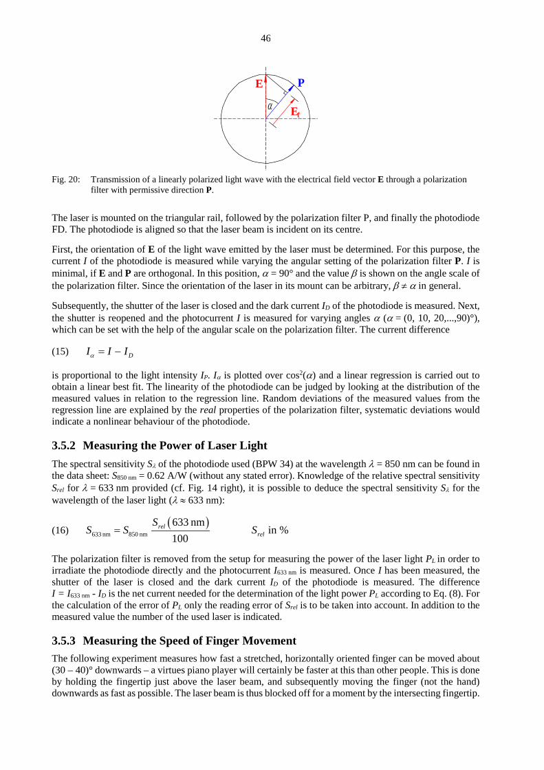
46

Fig. 20: Transmission of a linearly polarized light wave with the electrical field vector E through a polarization

filter with permissive direction P. The laser is mounted on the triangular rail, followed by the polarization filter P, and finally the photodiode FD. The photodiode is aligned so that the laser beam is incident on its centre. First, the orientation of E of the light wave emitted by the laser must be determined. For this purpose, the current I of the photodiode is measured while varying the angular setting of the polarization filter P. I is minimal, if E and P are orthogonal. In this position, α = 90° and the value β is shown on the angle scale of the polarization filter. Since the orientation of the laser in its mount can be arbitrary, β ≠ α in general. Subsequently, the shutter of the laser is closed and the dark current ID of the photodiode is measured. Next, the shutter is reopened and the photocurrent I is measured for varying angles α (α = (0, 10, 20,...,90)°), which can be set with the help of the angular scale on the polarization filter. The current difference

(15) DI I Iα = − is proportional to the light intensity IP. Iα is plotted over cos2(α) and a linear regression is carried out to obtain a linear best fit. The linearity of the photodiode can be judged by looking at the distribution of the measured values in relation to the regression line. Random deviations of the measured values from the regression line are explained by the real properties of the polarization filter, systematic deviations would indicate a nonlinear behaviour of the photodiode.

3.5.2 Measuring the Power of Laser Light The spectral sensitivity Sλ of the photodiode used (BPW 34) at the wavelength λ = 850 nm can be found in the data sheet: S850 nm = 0.62 A/W (without any stated error). Knowledge of the relative spectral sensitivity Srel for λ = 633 nm provided (cf. Fig. 14 right), it is possible to deduce the spectral sensitivity Sλ for the wavelength of the laser light (λ ≈ 633 nm):

(16) ( )

633 nm 850 nm

633 nmin %

100rel

rel

SS S S=

The polarization filter is removed from the setup for measuring the power of the laser light PL in order to irradiate the photodiode directly and the photocurrent I633 nm is measured. Once I has been measured, the shutter of the laser is closed and the dark current ID of the photodiode is measured. The difference I = I633 nm - ID is the net current needed for the determination of the light power PL according to Eq. (8). For the calculation of the error of PL only the reading error of Srel is to be taken into account. In addition to the measured value the number of the used laser is indicated.

3.5.3 Measuring the Speed of Finger Movement The following experiment measures how fast a stretched, horizontally oriented finger can be moved about (30 – 40)° downwards – a virtues piano player will certainly be faster at this than other people. This is done by holding the fingertip just above the laser beam, and subsequently moving the finger (not the hand) downwards as fast as possible. The laser beam is thus blocked off for a moment by the intersecting fingertip.

E P

αtE

47

The (time) period of intersection is measured with the photodiode and shall serve as a measure of speed. The influence of finger thickness is neglected. The measurement is to be done using a digital storage oscilloscope operated in the SINGLE-SEQ-mode. A requirement for this is the transformation of the photocurrent I into a voltage U. The easiest way to achieve this is to let I flow through a resistor R and measuring the voltage drop over the resistor using U = RI 20. Additionally, in order to reduce the time constant, the photodiode must be operated with a reverse voltage US (cf. Chap. 2.5.2). This is the prerequisite for the measurement of rapid changes in light intensity. Fig. 21 shows the associated circuit diagram.

Fig. 21: Circuit configuration for a photodiode for measuring rapid changes in light intensity IL as a function of time t. The temporal course of the voltage, U(t) ~ IL(t), may be recorded by a digital storage oscilloscope.

To create the setup according to Fig. 21, the resistor R ≈ 50 Ω is soldered to the circuit board and fitted with a connecting cable (in addition to the photodiode). The block voltage should be Us = 10 V. Once this has been completed, the measurement is carried out for the index finger and the ring finger of the right- and left hand. Question 4:

Are there any significant differences in the results?

4 Appendix

Tab. 1: Selected characteristics of the used sensors as far as available or possible to indicate.

Quantity Type Measuring range Resolution Response

time Noise

Force U-OL 227/10 (0 – 100) mN < 0.5 ms

± 0.7mV

Pressure SENSORTECHNICS

HCLA 12X5DB

(0 – 1250) Pa 0.5 ms ± 4 mV

Distance BAUMER OADM

12U6460/S35 (16 – 120) mm (0.002 –

0.12) mm21 < 0.9 ms < ± 5 mV

Angle TWK-

ELEKTRONIK PBA 12

(0 – 360)° 0.35° < 0.4 ms < 0.5°

Light power SIEMENS BPW 34 20 ns22

NEP23 4.1×10-14 W/Hz-1/2

20 In advanced measurement technology transimpedance amplifiers based on operational amplifiers are used for current/voltage

conversion. The required components are discussed in part II of the introductory laboratory course. 21 The smaller the distance between the LDS and the object under measurement, the better the resolution. 22 Depending on circuit set-up. 23 NEP: noise equivalent power.

+-Us

UR

47

Carl von Ossietzky University Oldenburg – Faculty V - Institute of Physics Module Introductory laboratory course physics – Part I

Force, Momentum, and Impulse of Force Keywords:

Force, resilience, HOOKE’s law, NEWTON’s axioms, momentum, impulse of force, harmonic oscillation, distance law for forces.

Measuring program: Calibration of a force sensor, force and displacement in a harmonic oscillation, force of attraction between magnets, impulse of force and change of momentum at an elastic collision on an air cushion track.

References:

/1/ DEMTRÖDER, W.: „Experimentalphysik 1 – Mechanik“, Springer-Verlag, Berlin among others /2/ MESCHEDE, D. [Ed.]: "Gerthsen Physik", Springer, Berlin among others

1 Introduction

This experiment mainly deals with the quantitative measurement of forces. In the first part, the relationship between force and deflection in a mechanical harmonic oscillation is investigated. The second part of this experiment deals with the distance law in the dynamic effect between two magnets. The third and final part explains the relationship between force and momentum and impulse of force, respectively.

2 Theory

2.1 Harmonic Oscillation: Force and Deflection Let us observe a set-up according to Fig. 1, which we have already got to know in the experiment “Sensors for force…“ in a similar form. A spring FE is attached to a force sensor S. A sphere K is suspended on the lower end of the spring via a rod ST. Additionally, a reflective disc R is mounted on the rod.

Fig. 1: Set-up for measuring the force and deflection in a harmonic oscillation. For notations cf. text. When the sphere is at rest, there is an equilibrium in the force of gravity of ST, K and R that points downwards and the resilience pointing upwards. The center of the sphere is then in its equilibrium position at x = 0. An additional force F0, which points downwards, deflects the sphere downwards by the distance x0 1. At time t = 0, the sphere is released and is accelerated upwards by the tensile force F of the spring. According to HOOKE’S law with the spring constant D we thus obtain for F: 1 Since F0 and all other observed forces act only in x-direction, a description with scalar quantities is sufficient.

K

FE

LDS

RST

S

xx0

0F0

48

(1) 0F D x= − Subsequently, the sphere performs a harmonic oscillation in the x-direction. The deflection from its equi-librium position, x(t), which can be measured using a laser distance sensor LDS, is described by the fol-lowing equation neglecting friction effects2:

(2) ( ) ( )0 cosx t x tω= where ω is the angular frequency of the oscillation which is given by:

(3) Dm

ω =

m is the decisive mass for the oscillation, given by:

(4) K ST R FE13

m m m m m= + + +

mK, mST, mR and mFE are the masses of the sphere, the rod, the reflective disc and the spring3 respectively. The velocity v(t) of the sphere is obtained by differentiating x(t) for time:

(5) ( ) ( )0 sinv t x tω ω= − The acceleration a(t) is obtained by differentiating the velocity for time:

(6) ( ) ( )20 cosa t x tω ω= −

Hence it follows for the force F(t) exerted on m by the spring:

(7) ( ) ( ) ( ) ( )20 0cos cosF t m a t m x t F tω ω ω= = − = −

with

(8) 20 0F m x ω=

Question 1: - The force F(t) has a positive or a negative sign depending on the position x(t) of the sphere. Within

which range does the spring act as a tension spring or as a pressure spring? At the equilibrium position of the sphere, the force sensor S measures the weight G of FE, ST, R, and K. If the sphere is pulled down from its position of rest by the force F0, S measures the force according to NEWTON’S 3rd axiom4 actio = reactio (9) ( )S 0 0F G F G F t= + = − = with F(t) according to Eq. (7). After the sphere has been released, S measures the force

(10) ( ) ( )SF t G F t= − After subtraction of G, S thus yields F(t) according to Eq. (7) with reversed sign.

2 A detailed mathematical description of the oscillation is given later on in the experiment “Forced mechanical oscillations“. 3 The relationship according to Eq. (4) is explained in the experiment “Forced mechanical oscillations“. 4 ISAAC NEWTON (1643 – 1727)

49

2.2 Distance Law for Magnetic Force As is generally known, the gravitational force FG between two masses m1 and m2 at distance r is defined by NEWTON’s law of gravitation:

(11) 1 2G 2

ˆm mGr

=F r

where G is the gravitational constant and r is the unit vector parallel to the connecting line between the center of both masses5. As the force decreases with the square of the distance r, this is called a 1/r2 law. Also the COULOMB law, which describes the force FE between two electrical charges q1 and q2 in a vacuum, is a 1/r2 law. It reads:

(12) 1 2E 2

0

1 ˆ4π

q qrε

=F r

where ε0 is the electric constant and r and r are defined in analogy to the law of gravitation. We obtain an attracting force for charges with unequal signs and a repulsive force for charges with equal signs.

Fig. 2: The distance law for magnetic forces. P1 and P2 represent the pole strengths of the magnets with diameters

that are small compared to their lengths. The distance r between the two magnets is measured between the poles.

Under certain conditions, a 1/r2 law is valid for the force between two magnets, too. Let us consider two bar magnets according to Fig. 2, the diameters of which are small compared to their lengths. Under this condition, the “strength” of such magnets can be described by pole strengths P that act with different signs at the magnetic north and south pole of the respective magnet and can be assumed to be point-like6. The force between two magnets is then described by COULOMB‘S law for magnets:

(13) 0 1 2M 2

ˆ4π

P Pr

µ=F r

where µ0 is the magnetic constant and r and r are defined in analogy to the law of gravitation. The force is attractive in cases of opposite poles and repulsive in cases of like poles.

2.3 Momentum and Impulse of Force The state of motion of a body of mass m moving linearly at a uniform velocity v, is described by the momentum (14) m=p v According to NEWTON’s 1st axiom, a change of the momentum is only possible, if a force F acts on the body. According to NEWTON’s 2nd axiom, the temporal change of the momentum caused by F is given by

(15) ddt

=pF

5 To be exact, Eq. (11) is only valid for point-like masses at distance r. However, the same relationship is found in approximately

sphere-like masses with symmetrical mass distribution around the center (e.g. in the system earth and moon). Then r describes the distance between both centers.

6 The magnetic pole strength P is defined differently in the literature. Here, it denotes the quantity with the unit [P] = A m.

r

P1 P2

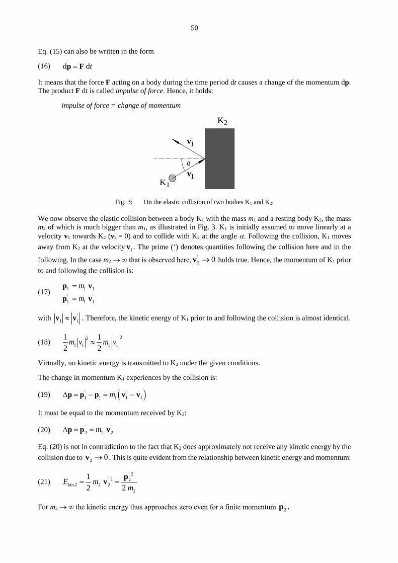
50

Eq. (15) can also be written in the form (16) d dt=p F It means that the force F acting on a body during the time period dt causes a change of the momentum dp. The product F dt is called impulse of force. Hence, it holds: impulse of force = change of momentum

Fig. 3: On the elastic collision of two bodies K1 and K2. We now observe the elastic collision between a body K1 with the mass m1 and a resting body K2, the mass m2 of which is much bigger than m1, as illustrated in Fig. 3. K1 is initially assumed to move linearly at a velocity v1 towards K2 (v2 = 0) and to collide with K2 at the angle α. Following the collision, K1 moves away from K2 at the velocity '

1v . The prime (‘) denotes quantities following the collision here and in the

following. In the case m2 → ∞ that is observed here, '2 0→v holds true. Hence, the momentum of K1 prior

to and following the collision is:

(17) 1 1 1' '1 1 1

mm

=

=

p vp v

with '1 1≈v v . Therefore, the kinetic energy of K1 prior to and following the collision is almost identical.

(18) 22 '

1 1 1 11 12 2

m v m v≈

Virtually, no kinetic energy is transmitted to K2 under the given conditions. The change in momentum K1 experiences by the collision is:

(19) ( )' '1 1 1 1 1m∆ = − = −p p p v v

It must be equal to the momentum received by K2:

(20) ' '2 2 2m∆ = =p p v

Eq. (20) is not in contradiction to the fact that K2 does approximately not receive any kinetic energy by the collision due to '

2 0→v . This is quite evident from the relationship between kinetic energy and momentum:

(21) ' 2

' 2 2kin,2 2 2

2

12 2

E mm

= =pv

For m2 → ∞ the kinetic energy thus approaches zero even for a finite momentum '2p .

K1

K2

v1

v1'

α

51

The change of momentum ∆p of K1 must be equivalent to the total (integral) impulse of force that K2 exerts on K1 during the collision process. According to Eq. (16) this impulse of force is given by:

(22) ( )0

dt tτ

∆ = ∫p F

Here, F(t) is the force acting during the time period τ of the collision. Initially, it acts as a brake on K1 reducing its velocity v1 to 0 and thereafter accelerates it to velocity '

1v . In order to understand the collision process better, we can imagine K2 to be a spring pressed together by K1 until its velocity is 0 and then relaxing again thereby accelerating K1 to velocity '

1v .

3 Experimental Procedure

Equipment: Force sensor working on DMS principle (measuring range (0 - 5) N), measuring amplifier for force sensor, set of weights for calibrating the force sensor, 2 power units (PHYWE (0 - 15 / 0 - 30) V), digital oscilloscope TEKTRONIX TDS 1012 / 1012B / 2012C / TBS 1102B, spring with sphere, rod and reflective disc, laser distance sensor (BAUMER OADM 12U6460/S35), bar magnets in Al mountings with stay bars, PVC distance piece, guide for bar magnet, adjustable table, air cushion track, sled for air cushion track with screen and Al cubes, hybrid light barrier (BETA-SENSORIK GLS-30BP/R), hook for force sensor, stand on base, rods, pillar of stand, cross joints, caliper gauge.

3.1 Calibration of the Force Sensor The force sensor used in the following experiment works on the same principle as the sensor used in the experiment “Sensors for force…“. These two sensors differ only in their measuring range (here: 5 N, pre-viously: 100 mN)7. The calibration of the sensor is performed using at least five mass pieces within the range m ≈ (50 – 500) g. The output voltage U of the force sensor8 is measured with an oscilloscope9. U is plotted over G = mg using the value g = 9.8133 m/s2 for the earth’s acceleration g that can be assumed to be exact. A regression line is drawn through the data, whose parameters are later used for converting voltage to a force.

3.2 Force and Deflection for a Harmonic Oscillation

The force F(t) and the deflection x(t) for a harmonic oscillation are to be measured using a set-up according to Fig. 1. First, the masses of the spring and of the system rod/reflective disc/sphere are determined by weighing. Then, all the components are attached to the force sensor, which is mounted on a stand as shown in Fig. 1. The laser distance sensor LDS is also attached to the stand and its position is adjusted such that the reflective disc remains within its measuring range during the oscillation. Subsequently, the sphere is manually pulled downwards by about 20 m as vertically as possible and then released. The output voltage of the LDS, ULDS(t), and the output voltage of the force sensor, US(t), are recorded with a storage oscilloscope triggered to ULDS. The time-base of the oscilloscope is adjusted so that 5 - 10 oscillation periods are visible on the screen. Following the transient oscillation a typical oscillation process is stored in single-sequence mode. A screenshot is taken and attached to the report.

7 Βecause of this reason the damping must be switched off. 8 To simplify matters, the term “output voltage of the force sensor“ is used here and in the following for the output voltage of

the measuring amplifier connected with the actual force sensor. 9 Since the voltage U is measured with the oscilloscope in the following measurements, U is also measured with the oscilloscope

instead of a multimeter here, in order to avoid differences between the measured values caused by different calibrations of oscilloscope and multimeter.

52

With the aid of the time cursors, the period of the oscillation is determined and the angular frequency ω is calculated. The amplitudes (index 0) of ULDS(t) and US(t) of a selected partial oscillation are measured using the voltage cursors: (23) ( ) ( )LDS,0 LDSmax LDS,min ,0 S,max S,min/ 2 / 2SU U U U U U= − = − With the calibration factor k of the LDS for voltage differences, 0,0962 V/mmk = , which is assumed to be exact, the oscillation amplitude x0 can be extracted and the force F0 can be calculated with Eq. (8). Mass m is calculated according Eq. (4) and ω is measured by an oscilloscope. From Us,0 and the calibration function of the force sensor F0 can also be estimated. Both results should be compared. Question 2: - What could be the reasons for differences of both quantities?

3.3 Force of Attraction Between two Magnets Using a set-up according to Fig. 4 we examine the validity of the distance law for the force of attraction between two magnets according to Eq. (13). Both magnets are mounted in aluminum tubes which are screwed to rods. Initially, only the upper magnet, with the pole strength P1, is attached to a force sensor S together with the rod. An almost frictionless guide A confines its motion to a vertical direction. The output voltage US,0 of the force sensor is measured. This voltage US,0 corresponds to the case r → ∞, hence only caused by the weight G of rod and magnet. From US,0 G is calculated with the data of the calibration function and subtracted from all other forces measured later on.

Fig. 4: Set-up for measuring the attraction force between two magnets with the pole strengths P1 and P2. All

components are mounted on one stand ST enabling a precise vertical mounting. For other notations refer to the text.

Subsequently, the lower magnet with the pole strength P2 is mounted on an adjustable table V, so that it can be moved in vertical direction. First, the lower magnet is adjusted so that the longitudinal axes of both magnets exactly superimpose each other. Then, a defined distance l is set between both magnets using a PVC piece (length l ≈ 20 mm, to be measured). The respective scale position of the shiftable table is noted down and defined as s = l. Then, the shiftable table is adjusted to the scale position s = 10 mm and US(s) is determined10. Subsequently, we reduce s to about s = 2 mm in steps of approx. 0.5 mm measuring again US(s) each time. The values of US(s) are converted into forces F(s) with the data of the calibration function. After subtracting G we obtain the forces FM(s) caused by magnetic attraction: 10 Example: Let l = 20.1 mm. At this distance between P1 and P2 the scale position 74.5 mm is read at the shiftable table V. This

value is defined as s = l = 20.1mm. Afterwards V shall be moved to the position s = 10 mm. Accordingly a value of (74.5 – 10.1) mm = 64.4 mm has to be adjusted at its scale.

AS

P2

P1 rV

ST

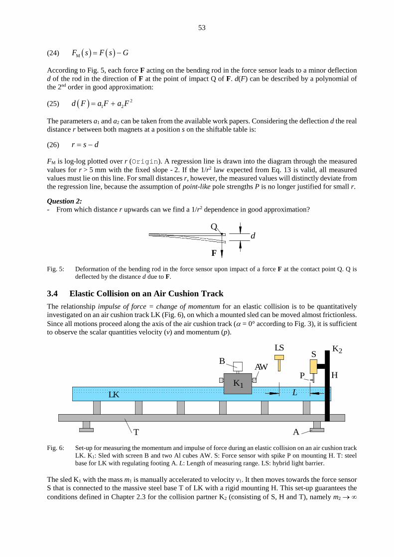
53

(24) ( ) ( )MF s F s G= − According to Fig. 5, each force F acting on the bending rod in the force sensor leads to a minor deflection d of the rod in the direction of F at the point of impact Q of F. d(F) can be described by a polynomial of the 2nd order in good approximation:

(25) ( ) 21 2d F a F a F= +

The parameters a1 and a2 can be taken from the available work papers. Considering the deflection d the real distance r between both magnets at a position s on the shiftable table is:

(26) r s d= − FM is log-log plotted over r (Origin). A regression line is drawn into the diagram through the measured values for r > 5 mm with the fixed slope - 2. If the 1/r2 law expected from Eq. 13 is valid, all measured values must lie on this line. For small distances r, however, the measured values will distinctly deviate from the regression line, because the assumption of point-like pole strengths P is no longer justified for small r. Question 2: - From which distance r upwards can we find a 1/r2 dependence in good approximation?

Fig. 5: Deformation of the bending rod in the force sensor upon impact of a force F at the contact point Q. Q is deflected by the distance d due to F.

3.4 Elastic Collision on an Air Cushion Track The relationship impulse of force = change of momentum for an elastic collision is to be quantitatively investigated on an air cushion track LK (Fig. 6), on which a mounted sled can be moved almost frictionless. Since all motions proceed along the axis of the air cushion track (α = 0° according to Fig. 3), it is sufficient to observe the scalar quantities velocity (v) and momentum (p).

Fig. 6: Set-up for measuring the momentum and impulse of force during an elastic collision on an air cushion track

LK. K1: Sled with screen B and two Al cubes AW. S: Force sensor with spike P on mounting H. T: steel base for LK with regulating footing A. L: Length of measuring range. LS: hybrid light barrier.

The sled K1 with the mass m1 is manually accelerated to velocity v1. It then moves towards the force sensor S that is connected to the massive steel base T of LK with a rigid mounting H. This set-up guarantees the conditions defined in Chapter 2.3 for the collision partner K2 (consisting of S, H and T), namely m2 → ∞

F

dQ

A

LSS

K1

BAW

P

LK

T

L

H

K2

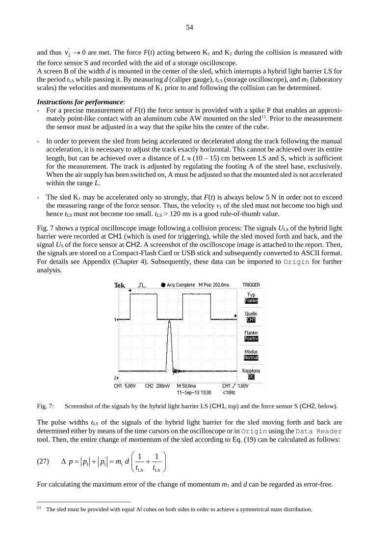
54

and thus '2v → 0 are met. The force F(t) acting between K1 and K2 during the collision is measured with

the force sensor S and recorded with the aid of a storage oscilloscope. A screen B of the width d is mounted in the center of the sled, which interrupts a hybrid light barrier LS for the period tLS while passing it. By measuring d (caliper gauge), tLS (storage oscilloscope), and m1 (laboratory scales) the velocities and momentums of K1 prior to and following the collision can be determined. Instructions for performance: - For a precise measurement of F(t) the force sensor is provided with a spike P that enables an approxi-

mately point-like contact with an aluminum cube AW mounted on the sled11. Prior to the measurement the sensor must be adjusted in a way that the spike hits the center of the cube.

- In order to prevent the sled from being accelerated or decelerated along the track following the manual

acceleration, it is necessary to adjust the track exactly horizontal. This cannot be achieved over its entire length, but can be achieved over a distance of L ≈ (10 – 15) cm between LS and S, which is sufficient for the measurement. The track is adjusted by regulating the footing A of the steel base, exclusively. When the air supply has been switched on, A must be adjusted so that the mounted sled is not accelerated within the range L.

- The sled K1 may be accelerated only so strongly, that F(t) is always below 5 N in order not to exceed

the measuring range of the force sensor. Thus, the velocity ν1 of the sled must not become too high und hence tLS must not become too small. tLS > 120 ms is a good rule-of-thumb value.

Fig. 7 shows a typical oscilloscope image following a collision process: The signals ULS of the hybrid light barrier were recorded at CH1 (which is used for triggering), while the sled moved forth and back, and the signal US of the force sensor at CH2. A screenshot of the oscilloscope image is attached to the report. Then, the signals are stored on a Compact-Flash Card or USB stick and subsequently converted to ASCII format. For details see Appendix (Chapter 4). Subsequently, these data can be imported to Origin for further analysis.

Fig. 7: Screenshot of the signals by the hybrid light barrier LS (CH1, top) and the force sensor S (CH2, below). The pulse widths tLS of the signals of the hybrid light barrier for the sled moving forth and back are determined either by means of the time cursors on the oscilloscope or in Origin using the Data Reader tool. Then, the entire change of momentum of the sled according to Eq. (19) can be calculated as follows:

(27) '1 1 1 '

LS LS

1 1p p p m dt t

∆ = + = +

For calculating the maximum error of the change of momentum m1 and d can be regarded as error-free.

11 The sled must be provided with equal Al cubes on both sides in order to achieve a symmetrical mass distribution.

55

For measuring the impulse of force the integral in Eq. (22) is replaced by a sum:

(28) ( )ii

p F t t∆ = ∆∑

where the F(ti) are the discrete values of the force sensor at times ti (sampling points of the oscilloscope) that can be calculated from the recorded voltage values US(ti) by applying the calibration function. The sum over the F(ti) is easy to determine using the Origin tool Statistics on columns12. ∆t is the constant temporal distance between two consecutive measuring values at times ti and ti+1, which results from the adjusted time-base sweep on the oscilloscope (x SEC/DIV) and the number of recorded measuring values (2,500).

(29) ( )10 DIV SEC/DIV / 2500t x∆ = × It is difficult to determine the start and end of the impulse of force, and thus its duration τ, precisely. Therefore, the sum according to Eq. (28) is not added up over τ, but over the complete time interval recorded, i.e. over all of the 2,500 measured values recorded with the oscilloscope. At this procedure we must take the following into account: Outside the time interval τ, F(ti) = 0 should be valid. Actually, F(ti) ≠ 0 can be caused by a small offset in the force signal and by electronic noise, which may lead to a significant error for summation over many ti. Therefore, we first calculate the mean F0 of the force signal over the time interval, which surely lies before the start of the collision13. Subsequently, this value F0 is subtracted from all measured values F(ti) and only then the sum is calculated according to Eq. (28). In order not to make the calculation of the maximum error of the impulse of force too elaborate, a maximum error of 5 mN may be assumed for each single force value F(ti) and the maximum error of Δt can be neglected Finally, we have to examine, whether the change of momentum according to Eq. (26) corresponds to the impulse of force according to Eq. (28). The reasons for possible deviations between both quantities are discussed.

4 Appendix

The following steps are necessary for storing data from the oscilloscope on an USB stick or Compact-Flash card, and for later converting them to ASCII data files: First, the following keys of the oscilloscope are pressed once: Basic adjustments:

SAVE/RECALL → Action → Save all PRINT → Save all Choose directory → Select GPRnn → Change directory → Back

Storage:

SAVE / PRINT After pressing the SAVE / PRINT key, four files are stored in the sub-directory ALLnnnn, where nnnn is a consecutive number (starting at 0000) that is increased by 1 each time the key SAVE / PRINT is pressed. The four files are:

12 Right mouse-click on the marked column, choose the menu Statistics on columns, tick Sum under the submenu

Quantities. 13 Mark lines in the column with values for F(ti), in which ti lies before the start of the collision. Then choose →

Statistics on columns, there choose submenu Quantities and tick Mean.

56

FnnnnTEK.SET ASCII file with operational parameters of the oscilloscope FnnnnTEK.TIF Image file with screenshot FnnnnCH1.CSV Data of CH1 (voltage U1 as a function of time t among others) FnnnnCH2.CSV Data of CH2 (voltage U2 as a function of time t among others)

For quantitative analysis, only the two last files available in CSV format are important.14 With the aid of the available Matlab script15 GPRTools.m, there option Tektronix CSV to ASCII, the signal courses U1(t) for CH1 and U2(t) for CH2 are extracted from these files and converted into ASCII format16. Subsequently, these data are stored in the directory ALLnnnn under the following file names:

FnnnnCH1_all.txt Column 1: t, column 2: U1(t) for CH1 FnnnnCH2_all.txt Column 1: t, column 2: U2(t) for CH2

These files can be imported to Origin via File → Import → … .

14 CSV is the abbreviation of character separated values. This means that the single entries in the file (numerical values, character

strings,…) are separated by a defined character. Here, the comma is the separating character. 15 After logging onto a PC in the laboratory the Matlab script is available under the working directory Q: MatlabSkripte$

(\\gpr00.gpr.physik.uni-oldenburg.de). 16 With newer versions of Origin, CSV files can be directly imported.

57

Carl von Ossietzky University Oldenburg – Faculty V - Institute of Physics Module Introductory laboratory course physics – Part I

Data Acquisition and Processing with the PC Keywords:

Continuous and discrete signals, sampling, sampling rate, sampling frequency,resolution, ana-log/digital conversion, weighing method, multiplexing, dual numbers, bit, digit.

Measuring program: Writing of a MATLAB-script for data acquisition with an A/D board, determination of the resolution of an A/D board, measurement of alternating voltages, calibration of a pressure sensor, measurement of temporal pressure changes.

References: /1/ Kose, V. [Hrsg.]; Wagner, S. [Hrsg.]: „Kohlrausch - Praktische Physik Bd. 3“, Teubner, Stuttgart, 1996

1 Introduction

In many physical experiments, the change of a value of a physical quantity G is to be acquired as a func-tion of time t. Such quantities may be e.g.: Pressure p, temperature T, intensity of radiation I, force F, acceleration a, among others. For recording G(t), sensors are used which convert the value of G(t) e.g. into a voltage signal U(t) (compare experiment “Sensors...”). Previously, so-called XT recorders were used to record the temporal course of U(t) on paper. Nowadays, PCs with data acquisition boards1 (hereafter DAB) are used instead, which register the course of U(t) digitally. In this experiment, the most important properties of such data acquisition boards and a software required for their control (exemplarily Matlab with the Data Acquisition Toolbox) are illustrated.

2 Basics of Data Acquisition

2.1 Continuous and Discrete Signals With a data acquisition board an analog voltage signal U(t) is transformed into a time series of numerical values N(i), i ∈ ℕ, that can be further processed with the PC. In general, the signal U(t) is neither restricted to certain voltage values nor to certain time values according to Fig. 1 (top). Therefore, it is called a time- and value-continuous signal. Even with very fast (and hence expensive) electronic components of a data acquisition board, voltage values U(t) can be recorded (sampled) only at discrete points in time ti at the interval

(1) Δt = ti – ti-1 i ∈ ℕ \ 0 The quantity ∆t is called sampling interval, the reciprocal value of this quantity,

(2) [ ] 11 sR Rt

−= =∆

is called sampling rate or sampling frequency and is given in samples/s or only in 1/s. The greater R, the better is the temporal resolution of the signal recording.

1 A data acquisition board is a card to be installed into a PC containing all electronic components necessary for its function that

can communicate with the rest of the hardware in the PC via the system bus (the entirety of data, address and control wires).

58

In practice, a restricted sampling rate is often used in order to reduce the amount of data to be stored. The question of how large R has to be chosen to enable the signal course to be recorded correctly will be investigated in detail later on in the experiment “Fourier analysis”. Due to R being restricted to ∆t > 0, and hence R < ∞ , a time-discrete signal U(ti) is generated by sampling U(t) as shown in Fig. 1 (middle). For better visibility, vertical lines are drawn in the diagram instead of data points whose lengths correspond to the individual voltages U(ti).

Fig. 1: Conversion of a value- and time-continuous voltage signal U(t) (top) into a time-discrete signal U(ti)

(middle) and a value- and time-discrete numerical sequence N(i) (bottom). The conversion of an analog voltage value U(ti) into a numerical value N(i) by means of an analog to digital converter (A/D converter, cf. Chap. 2.2) of a data acquisition board is not feasible at an arbitrary precision, but is restricted by the resolution A of the A/D converter. A is given in bit:

(3) A = m Bit, m ∈ ℕ For every data acquisition board, the measurable input voltage is restricted to an interval of the width

(4) max mineU U U= − For A/D conversion, m bit and thus 2m numerical values in the range between N = 0 and N = 2m – 1 are available for this voltage interval. Hence, the difference between two voltage values, the assigned numeri-cal values of which differ by just 1 (1 digit), is

t

U (t)

t

U (t )

i

i

N (i)∆U

∆ t

ti

59

(5) 2

em

UU∆ =

This quantity is also called the resolution of the A/D conversion. With ∆U > 0, the time-discrete signal in Fig. 1 (middle) becomes a time- and value-discrete signal by A/D conversion as shown in Fig. 1 (bottom). Within a maximum voltage range (e.g. ± 10 V), Ue may often be restricted to a smaller interval by soft-ware (cf. Table 1). This can be used to increase the resolution of the A/D conversion, if the input signal is known lie within this interval. An example for this: If the voltage interval is set to ± 10 V, then Ue = 20 V and, according to Eq. (5) (rounded to 4 significant digits): ∆U = 0.07813 V for m = 8 and ∆U = 0.0003052 V for m = 16. If the voltage interval is constrained to ± 0.5 V, then Ue = 1 V and higher resolution is achieved for an equal number of bits: ∆U = 0.003906 V for m = 8 and ∆U = 0.00001526 V for m = 16.

2.2 Principle of A/D Conversion Analog to digital converters (ADC) work on different principles. A conversion method frequently applied in data acquisition is the so-called weighing method working on the principle of successive approxima-tion. This method is schematically represented in Fig. 2. First, all m bits of the converter are set to 0. After that, the most significant bit (MSB) with the „number“ m and the significance 2m-1 is set to 1 on a trial basis. A voltage source contained in the A/D converter subsequently generates a voltage UD with the value

(6) [ ]12mDU k k V−= =

k being a proportional factor dependent on Ue. A comparator is used thereafter to verify

(7) ( ) ?i DU t U≥ If so:

• bit no. m continues to be set to 1, • bit no. m-1 is set to 1, too, • the internal voltage source generates a new voltage UD with the value

(8) ( )1 22 2m mDU k − −= +

If not:

• bit no. m is set back to 0, • bit no. m-1 is set to 1, • the internal voltage source generates a new voltage UD with the value

(9) 22mDU k −=

Thereafter, the validity of Eq. (7) is verified anew with the voltage UD from Eqs. (8) and (9), respectively, and depending on the result, bit no. m-1 is treated like bit no. m was treated before. Analogous steps are performed until the least significant bit (LSB) with the number 1 and the significance 20 has been obtained. In this way, the values 0 or 1 of the individual bits can be determined by means of successive approximation between U(ti) and UD. In the example from Fig. 2, the voltage level U(ti) (blue) is associated with the binary number 011 100 11, which is N = 115 in decimal representation. If we assume that Ue = 10 V, the binary number 111 111 11

60

(corresponding to N = 255) must be associated with the voltage level 10 V. This means, that for this value of Ue , we must have:

10 V255

k =

Fig. 2: Principle of A/D conversion according to the weighing method for an A/D converter with m = 8 bits. For the voltages UD generated by the A/D converter (red) that exceed the input voltage U(ti) (blue), the corresponding bits are set to 0. In the example, these are the bits having values 27, 23 and 22. The other bits are set to 1, since UD < U(ti) is fulfilled for the voltages UD.

Hence, under this prerequisite the binary number 011 100 11 from Fig. 2 corresponds to a voltage value U = k N = k × 115 ≈ 4,51 V. Each conversion process takes a certain time period tw, which increases linearly with the number m of bits. Therefore, ∆t ≥ tw must hold for the sampling interval ∆t from Eq. (1). Thus tw determines the mini-mal temporal distance between two successive samplings and hence the maximum sampling rate Rmax:

(10) max1

w

Rt

=

The described weighting process only works, if U(ti) does not change appreciably over the time tw. Hence, it is necessary to guarantee that U(t) remains nearly constant over temporal intervals of width of tw before a signal U(t) is recorded by a data acquisition card.

2.3 Multiplexing Normally, data acquisition boards have several signal inputs (channels) of which M are used depending on the application. In most cases, however, only one A/D converter is available on the boards. Sampling of the M input signals must then be done in the so-called multiplexing mode. At first, the signal at channel 1 is sampled, then with a temporal delay of tw each the signal at channel 2, the signal at channel 3 and so on, until channel M has been reached. After the time ∆t has passed, the process starts anew with the signal at channel 1. This has the consequence that the maximum sampling rate Rmax is reduced to Rmax/M per channel in that case. tw being the minimal time difference between two samples, an actually simultaneous sampling of two or more signals is not feasible in the multiplexing mode. In practice, however, the time difference tw is often small compared to the time in which the input signals vary appreciably, so that it can be neglected.

D

U(t )i

U

0 0 01 1 1 1 1LSBMSB

Bits auf 0, da U > U(t )D i

27 26 25 24 23 22 21 20

ZustandWertigkeit

115

N

8 4 37 6 5 2 1 Bit-Nr.

61

An example will illustrate this fact (Fig. 3). Two signals U1(t) and U2(t) are to be recorded simultaneously at a sampling rate of R = 1 kHz. The temporal distance between successive sample values of U1 and U2 shall thus be ∆t = 1 ms. The A/D converter of the data acquisition board is assumed to allow a maximum sampling rate of Rmax = 250.000 s-1, the minimal temporal distance between two samplings thus being tw = 4 µs. The first value of the signal U1(t) is assumed to be recorded at time t = 0, the first value of sig-nal U2(t) is then recorded at time t = tw. Sampling of the second value of U1(t) is done at time t = ∆t, the second value of U2(t) at time t = ∆t + tw and so on. As tw << ∆t, it is a good approximation in this exam-ple to speak of ”simultaneous“ sampling.

Fig. 3: “Simultaneous” acquisition of two voltage signals U1(t) and U2(t) using a single data acquisition board

operated in multiplex mode. Refer to the text for details.

2.4 Connection Types for Voltage Signals

The channels of a data acquisition board can usually be connected differently. In the simplest operation mode, the single-ended mode (SE mode, or grounded-source mode: GS), all M input voltages Uj(t) (j = 1,…,M) are referred to the case ground potential of the DAB, cf. Fig. 4, left2. This mode involves two disadvantages:

1. Fluctuations in the case ground potential affect the measured potential difference between the connector j and the case ground.

2. All input voltages Uj must have a common reference potential, as in Fig. 5 (left) the voltages U1 and U2 with the case ground as reference potential.

If the input voltages Uj do not have a common reference potential3, as e.g. the partial voltages Uj on the resistances of a voltage divider according to Fig. 5 (right), the differential operation mode (DI mode, or floating-source mode: FS) has to be used (Fig. 4 right). In this mode, the potential differences between two separate supply contacts each are recorded for each channel. The advantages of this mode are:

1. Identical potential fluctuations at both supply terminals of a channel4 do not affect the measured signal, because only the potential difference U between the supply terminals is measured.

2. The input voltages Uj can have different reference potentials; there is no common reference potential.

However, the DI mode also produces one disadvantage. Since each DI input requires two separate con-tacts on the data acquisition board, the number of DI inputs is only half the number of SE inputs.

2 This is equivalent to the measurement of two voltages with a two-channel oscilloscope, for which the outer contacts of the

BNC-socket connectors lie on the same potential. 3 Such signals are also called floating source (FS) signals. The name comes from the fact that there is no common fixed

reference potential. On the contrary, the potentials of both contacts can float at constant potential difference (voltage). Example: A potential difference of (5 V - 0 V) = 5 V yields the same measurement result as the difference (100 V – 95 V) or (1.000 V – 995 V).

4 Potential fluctuations can e.g. be caused by feed throughs into the connecting cables which connect a sensor to the data acquisition board.

t

U(t)U1

U2

∆ ttw

0

62

Fig. 4: Left: SE signal connection with the case ground (⊥) of the data acquisition board as reference potential

(grounded source, GS). Right: DI signal connection without reference to a potential of the data acquisition board (floating source,

FS).

Fig. 5: Voltage source U with connected resistances Rj and loads Lj. Left: Partial voltages Uj with common reference potential (ground). Right: Partial voltages without common reference potential. Voltmeters for measuring the partial voltages are shown in red.

3 Characteristics of Data Acquisition Boards

Data acquisition boards supplied by NATIONAL INSTRUMENTS (NI) are used in the introductory laboratory course. The most important characteristics of these cards are listed in Table 1. Fig. 6 shows as an example a photo of the board NI PCI 6221. Besides A/D conversion, the data acquisition boards can also be used for D/A conversion. Hence, it is possible to convert computer-generated signals into analog voltage signals which are available at an ana-log output of the board. This option, however, is of no importance for the present and is therefore not described in further detail. Parameter NI PCI 6014 NI PCI 6221 A/D converter type successive approximation successive approximation Number of inputs 16 SE / 8 DI 16 SE / 8 DI Maximum sampling rate Rmax / s-1 200.000 250.000 Resolution A / Bit 16 16 Input coupling DC DC Input resistance / GΩ 100 10 Input capacity / pF 100 100 Range of input voltage / V (adjustable by software) ± 0.05, ± 0.5, ± 5, ± 10 ± 0.2, ± 1, ± 2, ± 10

Table 1: Characteristics of data acquisition boards used in the introductory laboratory course.

U U

SE / GS DI / FS

Gehäuse

U

U U1 2

R1 R2 R1 R2 R3 R4

U1 U2 U3 U4

UL1 L2 L0

63

Fig. 6: Photo of the data acquisition board NI PCI 6221 (ref.: NI).

4 MATLAB-Software for Controlling Data Acquisition Boards

In the Introductory laboratory course, the software Matlab with the Data Acquisition Toolbox is used to control the NI data acquisition boards specified in Chapter 3. The interface between the opera-tion system of the PC (Windows 7) and the Matlab software is the driver NI-DAQmx. The following list states the Matlab commands to be used to read a voltage signal into the PC, to pro-cess it and to store it via a NI-DAB. All Matlab commands (starting with >> ) and the related state-ments in the Command window are set in the typeface Courier, while the respective comments appear in the typeface of the body text (Times Roman). >> clear Clear Matlab workspace

>> close('all','hidden') Close all figures

>> HW=daqhwinfo; daqhwinfo stands for data acquisition hardware

information: Get information about the data acquisition hardware installed in the PC and store it into the structure5 „HW”. „HW” contains several fields.

>> HW.InstalledAdaptors Read content of field „InstalledAdaptors“ of the structure HW. This field contains the Matlab names of the data acquisition components installed in the PC

ans = 'nidaq' 'parallel' 'winsound'

NI-DAB Parallel interface of the PC Soundcard of the PC

>> NI=daqhwinfo('nidaq'); Read information about the NI-DAB and store it into the structure „NI“

>> NI.BoardNames ans = 'PCI-6221'

Query the content of the field „BoardNames“ of the structure NI. This field contains the type name of the NI-DAB, here „PCI 6221“

>> NI.InstalledBoardIds Read content of field „InstalledBoardIds“. This field 5 For details on structures, please refer to the appendix (Chap. 6).

64

ans = 'Dev1'

contains the Matlab identification (ID) of the NI-DAB, here „Dev1“ (Device 1)

>> AI=analoginput('nidaq','Dev1'); Generate analog input object „AI“. After generation „AI“ establishes the connection between Matlab and the DAB.

>> addchannel(AI,0); Connect input channel 0 of the DAB with the analog input object AI. The input voltage range is preset to ± 10 V.

>> R=1000; Choose sampling rate R, here e.g. 1000 / s

>> set(AI,'SampleRate',R); Set (‚SampleRate‘) R on the data acquisition board

>> N=1000; Choose number N of voltage values to be read, here e.g. N = 1000

>> set(AI,'SamplesPerTrigger',N); Set N (‚SamplesPerTrigger‘) on the data acquisition board

>> start(AI) Start measurement

>> [U,t]=getdata(AI); Read voltage and corresponding time values from PC-memory6 and store data into the variables U and t. U and t are column vectors.

>> U_Mean = mean(U) U_Mean = ...

Calculate the mean Umean of the elements of U and write it into the command window.

>> sigma_U = std(U) sigma_U = ... >>sigma_U_Mean = std(U)/sqrt(N) sigma_U_Mean = ...

Calculate the standard deviation σU of U and write it into the command window. Calculate the standard deviation Uσ of the mean of U and output it in the command window.

>> Daten(:,1)=t; >> Daten(:,2)=U;

For data storage copy the column vectors U and t into the (N,2)-matrix „Daten“. Column 1: t, column 2: U.

>> save('MD.dat','Daten','-ascii'); Store matrix „Daten“ into ASCII file „MD.dat“. This file can be imported to Origin in order to generate a diagram of U(t).

>> plot(t,U); Plot U over t in order to receive a first summary of the measured data.

>> delete(AI); Delete input object. >> clear AI; Clear AI from workspace. Instead of typing the mentioned commands into the command window of Matlab line per line, it is more practical to enter the commands into a Matlab script file (m-file), to save the file and then to start it. For details, please refer to the Chapter „Usage of computers …“ of this script.

6 At first, the fed data are stored into a FIFO- (First-In-First-Out)- memory on the DAB (size of the FIFO-memory for the DAB

type NI PCI 6014: 512 measured values, type NI PCI 6221: 4096 measured values). From the FIFO-memory the data is transferred into the memory of the PC. This transfer is often realized by a direct connection between the DAB and the PC memory without using the CPU via Direct Memory Access, DMA.

65

In case it is known that a NI-DAB termed ’nidaq’ in Matlab is installed in the PC and that the Matlab identification of the DAB is ’Dev1’, some of the above-listed commands may be skipped. In that case, it is sufficient to enter the following lines into the m-file: clear close('all','hidden') AI=analoginput('nidaq','Dev1'); addchannel(AI,0); R=1000; set(AI,'SampleRate',R); N=1000; set(AI,'SamplesPerTrigger',N); start(AI) [U,t]=getdata(AI); U_Mean = mean(U) sigma_U = std(U) sigma_U_Mean = std(U)/sqrt(N) Daten(:,1)=t; Daten(:,2)=U; save('MD.dat','Daten','-ascii'); plot(t,U); delete(AI); clear AI; When the m-file is to be executed several times with different values of R and N in order to record differ-ent voltage courses (as in the experiment described below), it is useful not to alter the variables R and N as well as the file name, in which the data is to be saved, in the m-file each time, but to retrieve these variables via the command window after starting the script. For this purpose, the input command is used. The lines R=1000; N=1000; ... save('MD.dat','Daten','-ascii'); in the m-File must then be replaced by the following lines: R=input (' Sampling rate R in Hz: '); N=input (' Number N of sampling points: '); ... Name=input (' File name with extension.dat: ','s')7; save(Name,'Daten','-ascii'); Every input-command generates an output of the text in parenthesis in the command window and the system waits for an input via the keyboard. Every input is completed with the return key (↵).

5 Experimental Procedure

Equipment: Digital oscilloscope TEKTRONIX TDS 1012 / 1012B / 2012C / TBS 1102B, digital multimeter (AGILENT U1251B / U1272A), function generator (AGILENT 33120A / 33220A), PC with data acquisition board (NATIONAL INSTRUMENTS PCI 6014 PCI or PCI 6221) and accompanying BNC adapter (NATIONAL INSTRUMENTS BNC-2120), 9 V battery with connector, power supply (PHYWE 0 - 15 / 0 - 30) V, pressure sensor (SENSORTECHNICS HCLA12X5DB) on base plate with valves on mount, ERLENMEYER flask with smoothed plug on table, U-tube manometer with holder and reading scale (filled with water), beaker glass on support jack, flexible tubes and couplings, air balloon, kitchen paper roll.

7 By using the ‚s’ the fed characters are transferred as a text-variable (type character).

66

5.1 Operating the PC and the Data Acquisition Board Before turning on the PC make sure that the BNC adapter of type NI BNC-2120 (cf. Fig. 7) is hooked up to the data acquisition board of the PC (when the PC is running, this connecting cable must not be plugged in nor unplugged!). After turning on the PC, log in to the domain gpr with the known username and password. The BNC adapter makes it easy to connect the signals to be measured to the DAB by using coaxial cables. The adapter has 8 differential DI-inputs (labels dependent on the card type ACH 0,…, ACH 7, or AI 0,…, AI 7 respectively). In this experiment, signal sources (battery, power supply, pressure sensor) are, in general, only to be connected to the BNC input ACH 0, or AI 0 resp. The (slider) switch above the BNC input connector of ACH 0, or AI 0 must be in the position labeled „BNC”. The input-selector switch for the BNC input is set to FS („floating source”, cf. Chap. 2.4). The maximum input voltage range that the data acquisition board can withstand is ± 10 V; this range should not be exceeded. As a control, all of the input signals of the data acquisition board are therefore simultaneously displayed on the oscilloscope.

Fig. 7: Left: Photo of the BNC-adapter of type NI BNC-2120. Right: Sketch of the mounting jacks of the same

adapter (Ref.: NI).

5.2 Starting MATLAB Matlab is started by double click on the respective icon. In the Matlab menu line „Current Direc-tory“, the path „O:\Personal_Directory“ is set. With the commands described in Chapter 4, the designation (InstalledAdaptors), the type (BoardNames) and the Matlab identification (InstalledBoardIDs) of the data acquisition board are obtained.

67

Subsequently, a m-file is written, by means of which voltage signals can be read in, processed and saved. The m file is saved in the personal directory.

5.3 Measurement of a DC Voltage and Determination of the Resolution A 9 V battery is connected to the input channel of the DAB and in parallel with a multimeter. The voltage is read into the PC (R = 100 s-1 and N = 100 are good orientation values) and the mean and the standard deviation of the single measurement are determined from the N measured values Ui. The determined values are compared to the value measured with the multimeter and its maximum error. The Ui are plotted over i using Origin. It can be seen from the plot, that the Ui differ only by integer multiples of a voltage value ∆U. ∆U is determined and compared to the expected resolution of the DAB according to Eq. (5). Here sufficiently number of digits must be specified.

5.4 Measurement of AC Voltages A sinusoidal alternating voltage without direct current offset (frequency 50 Hz, amplitude 2 V) is gener-ated using a function generator (FG). The output of the FG is connected to the input channel of the DAB and in parallel with the digital oscilloscope and the multimeter. The voltage is read into the PC (R = 1,000 s-1 and N = 1,000 are good orientation values) and its peak-peak value Uss as well as its effec-tive value Ueff are determined. For both quantities error informations are not required. Uss is, in good approximation, determined by the difference between the maximum and the minimum of the acquired N voltage values Ui . The corresponding formula in Matlab-notation reads: U_ss = max(U) - min(U) Ueff is given by:

(11) 2eff

1

1 N

ii

U UN =

= ∑

or, in Matlab-notation:

U_eff = sqrt(sum(U.^2)/N)

(cf. Chapter „About the set-up of electric circuits..” of this script). This value is called the rms-value (root-mean-square value). The value of Uss recorded by the DAB is compared to the value measured with the oscilloscope and the effective value Ueff recorded by the DAB is compared to the value indicated by the multimeter and to the theoretical expectation. Both devices must be configured so (V/DIV on the oscilloscope, measuring range on the multimeter) that Uss ,and respectively Ueff can be measured with the highest possible resolution. The measurements described above are repeated with a square-voltage signal of the same frequency and amplitude.

5.5 Measurement of Pressure Differences A pressure sensor of the type HCLA12X5DB, which has already been used in the experiment “Sen-sors...”, is available for measuring pressure changes in gasses. Details about its operational principle and its usage are to be taken from the accompanying script.

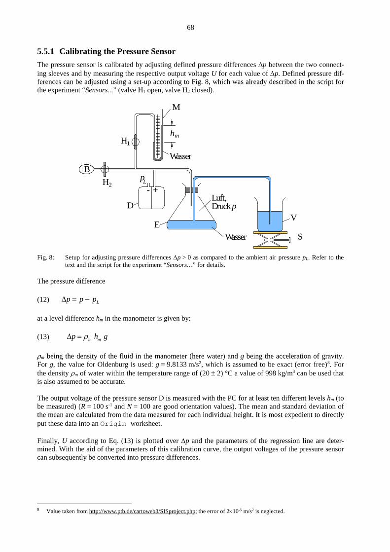
68

5.5.1 Calibrating the Pressure Sensor The pressure sensor is calibrated by adjusting defined pressure differences ∆p between the two connect-ing sleeves and by measuring the respective output voltage U for each value of ∆p. Defined pressure dif-ferences can be adjusted using a set-up according to Fig. 8, which was already described in the script for the experiment “Sensors...” (valve H1 open, valve H2 closed).

Fig. 8: Setup for adjusting pressure differences ∆p > 0 as compared to the ambient air pressure pL. Refer to the

text and the script for the experiment “Sensors…” for details. The pressure difference (12) Lp p p∆ = − at a level difference hm in the manometer is given by: (13) m mp h gρ∆ = ρm being the density of the fluid in the manometer (here water) and g being the acceleration of gravity. For g, the value for Oldenburg is used: g = 9.8133 m/s2, which is assumed to be exact (error free)8. For the density ρm of water within the temperature range of (20 ± 2) °C a value of 998 kg/m3 can be used that is also assumed to be accurate. The output voltage of the pressure sensor D is measured with the PC for at least ten different levels hm (to be measured) (R = 100 s-1 and N = 100 are good orientation values). The mean and standard deviation of the mean are calculated from the data measured for each individual height. It is most expedient to directly put these data into an Origin worksheet. Finally, U according to Eq. (13) is plotted over ∆p and the parameters of the regression line are deter-mined. With the aid of the parameters of this calibration curve, the output voltages of the pressure sensor can subsequently be converted into pressure differences.

8 Value taken from http://www.ptb.de/cartoweb3/SISproject.php; the error of 2×10-5 m/s2 is neglected.

Wasser

M

Luft, Druck p

EV

S

hm

Wasser

D

- +pLH

H1

2

B

69

5.5.2 Measurement of Temporal Pressure Changes For measuring temporal pressure changes with a set-up according to Fig. 8, the valve H2 is opened in addition to valve H1 to establish a connection between the balloon B and the air volume in E. An over-pressure in B is produced by raising the beaker glass V. Subsequently, the balloon is speedily squeezed together once and then released. While squeezing the balloon care must be taken that the maximum pres-sure difference of the sensor (∆p = + 1.25 × 103 Pa) is not exceeded and that the pressure at the „+”-con-nection of the pressure sensor remains always above the pressure of the ambient air. The latter condition is ensured as long as the water level in the right leg of the U-tube shown in Fig. 8 is higher than the water level in the left leg. The temporal course of the pressure difference while and after squeezing the balloon is to be recorded until the water level in the manometer is again stable at its initial level. This measurement is carried out twice. The recorded values of the output voltage of the pressure sensor are converted to pressure differences using the calibration data from Chap. 5.5.1. The results are plotted in diagrams ∆p(t) and analysed.

6 Appendix: Definition of a Structure in Matlab A structure is a named section of memory divided into fields. The individual fields of a structure can have different sizes. A field can hold just one element (e.g. a numerical value), or several elements in the form of a vector or a matrix9. The data contained in the elements of the structure’s fields can have different data types (also called classes in Matlab). Individual data types may be characters (data type charac-ter), integral numbers (data type integer), real numbers (data types single or double) etc. Each field and each element has its own label. An example to clarify the above: We will create a structure named student, which is to contain the fields name, surname, matriculation_number, subjects, and semester. Furthermore, the field subjects should contain an array of elements, while the other fields are to hold only one element each. The following Matlab-commands are used to save data to the individual elements (the period is the separator between structure and field, or field and element respectively): >> student.name = 'Mueller'; >> student.surname = 'Hans'; >> student.matriculation_number = 123456; >> student.subjects.a = 'Physik'; >> student.subjects.b = 'Mathematik'; >> student.subjects.c = 'Chemie'; >>.student.semester = 8; Since the data types for name, surname and subjects are character strings (data type character), the assigned values need to be placed within single quotes. After the data has been entered, one can issue the command >> student

to display how Matlab saved the structure:

student =

name: 'Mueller' surname: 'Hans' matriculation_number: 123456 subjects: [1x1 struct] semester: 8

9 A field may also be a structure containing structures, fields, or elements and so forth.

70

Since the field subjects contains more than one element, only the data type of the field (struct) is shown. To view the individual entries in subjects, the command >> student.subjects

needs to be issued. The Matlab output will be: ans =

a: 'Physik' b: 'Mathematik' c: 'Chemie' Fig. 9 shows a schematic representation of the structure student. For further details, refer to the Matlab documentation.

Fig. 9: Schematic representation of a structure in Matlab.

Mueller

Hans

123456789

Physik

Mathematik

Chemie

8

nachname

vorname

matrikelnr

semester

faecher

student

a

b

c

71

Carl von Ossietzky University Oldenburg – Faculty V - Institute of Physics Module Introductory laboratory course physics – Part I

Characterization of a Transmitter-Receiver System

Keywords: Microwaves, transverse waves, plane waves, spherical waves, standing wave, directional characteristic, reflection law and refraction law, index of refraction, polarisation. .

Measuring program: Properties of a transmitter-receiver system for microwaves, measurement of the distance dependence and directional characteristic, index of refraction of PVC for microwaves, reflection of microwaves at a metal plate and a wire grid, polarisation of microwaves.

References: /1/ DEMTRÖDER, W.: „Experimentalphysik 2 – Elektrizität und Optik“, Springer-Verlag, Berlin among others /2/ EICHLER, H. J., KRONFELDT, H.-D., SAHM, J.: „Das Neue Physikalische Grundpraktikum“, Springer-Verlag,

Berlin among others

1 Introduction Over the course of your studies of physics you will get to know different transmitter receiver systems, e.g. the system light source / photo detector in optics, or the system loudspeaker / microphone in acoustics. Such systems are generally described by a number of characteristic values. The aim of this experiment is to familiarize you with some of these values by measuring the characteristics of a transmitter receiver system for microwaves1. It is to be investigated in particular,

- whether, and if yes how, the intensity of the emitted wave decreases with increasing distance from the transmitter (distance dependence),

- in which geometric form (e.g. beam-like, spherical or lobar) the wave propagates (directional char-acteristic),

- by which structures the wave is reflected (reflection law), - whether the wave is refracted at the interface air → PVC (refraction law and index of refraction), - whether the wave is linearly polarized.

The system consists of a microwave transmitter and a suitable receiver. Both components are treated as ”black boxes” that serve a certain purpose (emit a wave and detect the intensity of a wave), the construction of which, however, is of no importance for the experiment and is therefore neglected. Fundamental school knowledge of optics is required to analyse parts of the tasks in this experiment: reflection, refraction, standing wave. In the course of the introductory laboratory course, these subjects will be treated in detail following their presentation in the lecture.

2 Experimental Procedure Equipment:

Microwave transmitter (Type I with Gunn diode MICROSEMI MO86751A, P ≈ 10 mW, λ ≈ 28.5 mm; type II with Gunn diode CL 8650 8927 (unknown manufacturer), P ≈ 15 mW, λ ≈ 27.5 mm), microwave receiver (HEWLETT-PACKARD X424A), 2 triangular rails (lengths 1.5 m and 0.5 m), joint for triangular rails with angle scale indicator, angle-sensor (TWK ELEKTRONIK PBA 12), 3 power supplies (PHYWE (0 – 15 / 0 – 30) V), multimeter (AGILENT U1272A or U1251B), digital oscilloscope TEKTRONIX TDS 1012 / 1012B / 2012C / TBS 1102B, PVC plate, metal plate, wire grid, transition stage (length 100 mm) with motor and laser distance sensor (BAUMER OADM 12U6460/S35), 2 impedance converters, PC with data acquisition board (NATIONAL INSTRUMENTS PCI 6014 or PCI 6221) and BNC-adapter (NATIONAL INSTRUMENTS BNC-2120), metal measuring tape (length 1 m), stand material.

1 Microwaves are electromagnetic waves in the frequency range between approx. 300 MHz and 300 GHz.

72

2.1 Set-up of Transmitter and Receiver Before starting with the experiments the operation of transmitter and receiver has to be learnt. For this purpose, a set-up according to Fig. 1 is constructed. Transmitter S and receiver E are assembled on a triangular rail (about 1.5 m long) adjusted to the same height and arranged centrically to the axis A at a distance of d = 5 cm from each other. The distance between the front edges of the horns of transmitter and receiver is defined as distance d.

Fig. 1: Schematic set-up of the transmitter S connected to a supply voltage UQ and the corresponding receiver E.

E is connected to the oscilloscope O and/or a data acquisition board via a coaxial cable, the outer conductor of which is grounded. A is the joining axis of S and E. For some experiments, S and E are mounted on a single triangular rail, for others two rails connected by an angular joint with rotational axis D are used. d is the distance between S and E, while the angular orientation is given by ϕ. The angle ϕ is measured using an angle-sensor, which is known from the experiment “Sensors…”.

The transmitter is connected to a DC power supply UQ that has been adjusted to an output voltage of 10 V beforehand (to be checked with a multimeter). It then emits a microwave with constant power P with the wavelength λ (P and λ see accessories). The receiver is connected to an oscilloscope O (DC coupling) and/or a data acquisition board (DAB) via a coaxial cable. It measures the intensity I of the incident microwave. Intensity means the temporal average of energy of a wave per time and area, the unit of intensity thus being [I] = J s-1 m-2 = W m-2. (The detector cannot directly follow the high-frequency course of the electric field E of the microwave (frequency approx. 10.5 GHz2).3) The receiver is constructed so that it converts the intensity I of the received wave into a negative voltage signal U: I ∼ -U. For the following experiments only the magnitude |U| of the voltage is decisive. Hints: - The outer conductor of the coaxial cable is grounded (connection with the ground terminal ( ) of the

laboratory), as to prevent the possible destruction of the semiconductor diode in the receiver by elec-trostatic discharge.

- Since, to an extent, the microwaves can also be scattered by, and reflected from experimenting persons, all of the following measurements should always be done under the same conditions (same standing place of persons etc.).

2.2 Distance Dependence First, the distance dependence is measured. For this purpose, the transmitter and receiver are mounted on one triangular rail (length about 1.5 m) according to Fig. 1 and the voltage U at the receiver is measured as a function of the distance d (5 cm ≤ d ≤ 1 m) with the oscilloscope. With varying d, an oscillation of the detected signal will occur, which is superimposed to the distance dependent course of the signal. This oscillation (period length λ/2) is due to the fact that part of the emitted wave is reflected by the receiver, interferes with the emitted wave and forms a standing wave. Since the amplitude of the reflected wave is significantly smaller than the one of the emitted wave, a standing wave with a weak modulation forms (cf. Fig. 2).

2 For comparison, frequencies of other microwaves: Digital-satellite TV approx. 12 GHz, microwave oven approx. 2.5 GHz. 3 This is analogous to a photo detector, which also can measure only light intensities, but not the temporal course of the electric field of a light

wave in the frequency range of 1014 Hz.

d

ϕ

S

OD

E

A= UQ

73

Fig. 2: Spatial course of the intensity I of a standing wave caused by interference of two plane microwaves

propagating in opposite directions with a wavelength of λ = 30 mm4. Blue: Course of the intensity for the case, that the amplitude E of the incident wave (Ea) is equal to the amplitude of the reflected wave (Er): Er = Ea. Red: Er = 0,2 Ea. Black: Er = 0. The maxima and minima of the intensity are spaced by a distance of λ/2 each, “a.u.” stands for arbitrary units.

For measuring the distance dependence it must be ensured that the measuring points are always at the distances di where the magnitude of the receiver signal, |U|, is maximal. The distance between measuring points should be 2λ. After a measuring point is adjusted, the measured value for U can be obtained from the oscilloscope by using the operation mode Measure → Average. For U, no error must be stated. The maximum error for di results from the restricted precision in determining the position of measuring points. For the analysis, |U| is plotted against d (with maximum error ∆d) once in a semi-log plot (|U| on logarithmic axis) and once in a double logarithmic plot. Additionally, the curves that would result for the following cases are plotted into the diagrams: a) The transmitter emits a strongly restricted ray which is not damped between S and E:

0 const.U U= = with the initial voltage |U0|.

b) Like in a), but with exponential damping by absorption between S and E: 0 e dU U α−= with the damping coefficient α.

c) The transmitter emits a spherical wave which is not damped between S and E by absorption: 2

0 /U U k d= . k is a scaling factor to be chosen so that |U| = |U0| for d → 0. By comparing the course of measured data with theoretically expected courses according to a) to c) it is to be determined, in which way the wave propagates. For presentation of the theoretical curves, suitable values have to be inserted for α, k and |U0| so that the expected course of the curve is clearly visible. In order not to draw false conclusions, the measured directional characteristic (Chapter 2.3) must be considered as well!

2.3 Directional Characteristics For the measurement of the directional characteristics the transmitter is mounted on the long rail, so that the front edge of the horn lies right on the rotation axis D (Fig. 1). The receiver is placed at a distance of about 40 cm behind the rotation axis on a second rail (about 0.5 m in length). Both rails are connected by a swivel joint. The angle ϕ can be read off from an angular scale and simultaneously be measured with the aid of an angle-sensor, which is already known from the experiment “Sensors...”. While adjusting the distance between E and D, it must be ensured that the receiver signal |U| shows a maximum for an angular orientation of ϕ = 180°. The angle ϕ = 180° is set by aligning the rails along their common axis A with the aid of a metal measuring tape. 4 The intensity I of an electromagnet wave is proportional to the square of the amplitude E of its electric field: I ~ E2.

74

Fig. 3: Example of a polar diagram for the function r(α) = 1 + cosα (red curve). The angle α runs counter-

clockwise. For every angle α, the function value r(α) is represented as the distance from the centre of the diagram (exemplarily marked by a blue line for α = 15°.

By rotation of the arm with the receiver E, the angle is increased from ϕ = 150° to ϕ = 210°. During the rotation, the output voltage UW of the angle-sensor and the voltage U at the receiver are measured and recorded with a DAB (see below Note for data acquisition with the DAB). Subsequently, |U| is presented as a function of ϕ (calculated from UW) in a polar diagram5 with the aid of Origin (cf. Fig. 3). No errors must be stated for |U| and ϕ. The polar diagram is presented as a line diagram instead of a point diagram, in order to account for the large amount of measured data, In addition, the curves which would result in cases a) and c) are drawn into this diagram. Note for data acquisition with the DAB The voltage UW of the angle-sensor and the voltage U at the receiver are measured and recorded simulta-neously by a data acquisition board (DAB) in the PC in an analogue manner to the experiment “Data acquisition with the PC...”. UW and U are fed to the connectors ACH 0 und ACH 1, or AI 0 und AI 1 resp., each via an impedance converter6 for reasons of signal matching. The Matlab-m-file from that experiment “Data acquisition…” must be extended in order to allow recording both signals simultaneously. The m-file is extended by one line (marked in red) to add a second channel (No. 1) next to channel No. 0 for data recording: addchannel(AI,0); (Channel 0: UW) addchannel(AI,1); (Channel 1: U) A sampling rate of R = 100/s is sufficient. By using the known command [UG,t]=getdata(AI); the data are read out following the end of the measurement. UG holds the voltage values from both channels in the form of an (N, 2)-matrix having N rows and 2 columns, where N is the number of recorded values. The first column holds the values measured at channel 0, thus the values of UW, the second column hold the values measured at channel 1, thus the values of U. The data for the time t are not needed for further analysis. The data for UW and U are exported into an ASCII-file (here: MD.dat) for further processing by Origin later on: save('MD.dat','UG','-ascii') 5 To create a polar diagram with Origin: → Plot → Specialized → Polar 6 The composition and function of impedance transformers are treated in the experiment “Operational Amplifier” later on (summer semester).

75

A quick glance (graph) of the course of U as a function of UW can be obtained by using the plot-command:

plot (UG(:,1),UG(:,2)) (The colon is used to select all data from column 1, or all data from column 2, respectively) .

Note for avoidance of interfering voltages:

This part of the experiment requires connecting the ground-wires (0 V) of the voltage supplies for the impedance transformer and angle-sensor to the ground terminal ( ) of the power supplies, in order to prevent disturbing voltages from the ground loops.

2.4 Refraction The aim of this partial experiment is the determination of a rule-of-thumb value for the refractive index nPVC of PVC for the used microwave7. The propagation velocity of electromagnetic waves depends on the index of refraction n of the medium through which the waves propagate. In vacuum, n = 1; in this case, the waves propagate at the speed of light in vacuum c. c is a universal constant (cf. back envelope of this script). In media (index M) with n > 1, the propagation velocity is lower. It holds:

(1) MM

ccn

=

In vacuum, the following relation between the propagation velocity c, the wavelength λ and the frequency ν of an electromagnetic wave holds: (2) c λ ν=

In a medium with M 1n > it holds likewise:

(3) M Mc λ ν= The propagation velocity and the wavelength are reduced inside a medium, while the frequency of the wave remains unchanged. The combination of (1) to (3) yields:

(4) M M

cn n

λ ν=

For air, M 1n ≈ , and hence, Mc c≈ and Mλ λ≈ .

The contraction of the wavelength in a medium with M 1n > can be exploited in order to measure the index of refraction Mn . For this purpose, we consider a cut-out of the standing wave previously known from Chap. 2.2 as depicted on the top in Fig. 4. Between S and E there is air with 1Airn ≈ . Along a distance of length L, M maxima of intensity form, separated by λ/2 from each other. It thus holds:

(5) 2

L M λ=

7 In the following description it is presupposed that the microwave propagates like a plane wave. Following the results from Chap. 2.3 this is not

the case. Furthermore, the measurement is influenced by scattering and reflection at surrounding materials. Therefore, it is not possible to measure nPVC precisely with the used set-up. However, the measurement delivers a usable rule-of-thumb value.

76

Fig. 4: Standing waves between S and E. The top shows the case where S and E are separated by air. The bottom shows the case where a plate of thickness D with the index of refraction Mn is inserted into the air between S and E, which shifts the maxima of intensity towards the plate within the range a. For other labels refer to the text.

Now, we insert a plate of thickness D between S and E according to Fig. 4 bottom. Let the index of refraction of the plate’s material be 1Mn > . This causes the wavelength inside the plate to be contracted:

(6) MMnλλ =

and the number of antinodes along the distance L to increase by m. It holds:

(7) M

22

D a M mλ λ+ = +

The increase of the number of maxima of intensity by m is, outside the plate, accompanied by an offset of the maxima by a distance l, for which holds:

(8) 2

l m λ=

Additionally, it holds according to Eq. (5):

(9) 2

L D a M λ= + =

By inserting M from Eq. (9) into Eq. (7) and together with Eqs. (6) and (8), it follows:

(10) ( )M 22 2 2D an D a l

λ λ λ λ+

+ = +

It thus follows for Mn :

(11) MD ln

D+

=

By measurement of D and l, it is thus possible to determine Mn . However, the method described above is only unambiguous, if m < 1. This is equivalent to l < λ/2. According to Eq. (11) this means:

lD

L

a

77

(12) ( )M 12

l D n λ= − <

and hence

(13) ( )M2 1

Dn

λ<

−

In this experiment, the index of refraction of PVC, PVCn , for a microwave with λ ≈ 28.5 mm and λ ≈ 27.5 mm, respectively, shall be determined with the aid of Eq. (11). The index of refraction for PVC is in the order of magnitude of PVCn ≈ 1.6. Thus it follows for both values of λ: D < 23 mm. Here, D ≈ 10 mm is used. In order to measure l, we proceed as follows: S and E are mounted on both triangular rails symmetrically to the rotating axis D at a distance of d0 = 500 mm. The receiver is mounted on a motorized translation stage V which allows it to be displaced along the axis A by 100 mm in the direction of S (Fig. 5). The motor is operated by a direct current. The speed of displacement depends on the height of the applied voltage (maximum 24 V), the direction of movement (forwards / backwards) is governed by the polarity. Both ends of the translation stage are fitted with micro-switches which cause the motor to stop upon reaching either endpoint.

Fig. 5: Set-up of transmitter S and receiver E on a motorized translation stage V. With this translation stage E can be moved forwards from the right to the left stop position and backwards from the left to the right stop position. In the stop positions sA and sB are the corresponding distances between the LDS and the ground plate on which E is mounted.

A laser distance sensor LDS that is known from the experiment “Sensors…“ is mounted on the translation stage. Its output voltage UL changes linearly with the translation of E. The sensor is calibrated by measuring the distances sA and sB (definition see Fig. 5) for both stop positions and the corresponding output voltages ULA and ULB. If E is at any position between the two stop positions during the translation, it follows for the momentary distance s of the receiver from the right stop position:

(14) ( )( ) B AL LA

LB LA

s ss U s UU U

−= −

−

and thus for the decisive distance d between S and E:

(15) 0d d s= − The motor is started at the right stop position and driven forward in the direction of S up to the left stop position. During the translation, the voltage UL and the voltage U at E are measured with the data acquisition board and saved (analogue to the procedure for the measurements of Chap. 2.3). Subsequently, the measurement is repeated with the PVC plate of thickness D0 (measure with caliper) inserted between S and E. The plate is mounted centric to the rotating axis D. In order to prevent the measurement from being disturbed by signal reflections, the plate is orientated in an angle of α = 45° to the axis A. Thus, the microwave propagates the distance

S E

sA

sB

d

LDS

V

0

A D

78

(16) ( )0 / cosD D α= in PVC8. After that, the motor is started in the left stop position and moves backwards to the right stop position. During the movement UL and U are recorded again and then stored. From the two datasets the distances d are calculated using Eqs. (14) and (15) with the aid of Origin. Subsequently, |U| is plotted over d in one diagram for both datasets. With the Origin-tool “Data coordinates / Data Reader“9, it is possible to determine the position of a selected maximum of intensity in both curves and its offset l from this. Finally, the index of refraction PVCn is determined from the values for l and D. Note for avoidance of interfering voltages:

This part of the experiment requires connecting the ground-wires (0 V) of the voltage supplies for the impedance transformer and laser distance sensor to the ground terminal ( ) of the power supplies, in order to prevent disturbing voltages from the ground loops.

2.5 Polarization In a linearly polarized microwave beam, the electrical field E of the wave oscillates in only one spatial direction (e.g. y-direction, cf. Fig. 6). If such a wave is incident on a metal wire grid oriented in the same direction, currents are induced in the rods, causing them to act as a HERTZian dipole. The wave emitted by the dipoles is phase shifted to the incident wave by 180°. Behind the grating, destructive interference occurs between the incident and the emitted waves. A receiver placed behind the grating will thus (if at all) measure only a weak signal.

Fig. 6: Interaction of a linearly polarized wave E with a wire grid whose thin rods are oriented in the direction of

polarization of the wave. In front of the grating the wave emitted backwards by the dipoles interferes with the incident wave. If the grating is tilted towards the incident wave as in the experiment on reflection (Chap. 2.6.2), the wave emitted backwards (the reflected wave) can propagate without interference from the incident wave. If the linearly polarized wave is incident on a grating where the rods are oriented perpendicular to the direction of polarization, no appreciable currents are induced (assuming the diameter of the rods is small). In this case, no HERTZian dipole radiation is emitted, allowing the incident wave to pass the grating nearly undisturbed. To analyse the polarization characteristics of the microwaves used in this experiment, S and E are mounted at a distance of d ≈ 5 cm (ϕ = 180°) from one another. A wire grid is held between S and E the rods of which are in the vertical direction one time and in the horizontal direction the next. The voltage U at the receiver is measured with the oscilloscope for each line orientation. Question 1: - Is the wave linearly polarized? If so: In which direction?

8 Approximation for a plane wave. 9 The graphical symbol for the tool Data Reader is .

E

t

y

79

2.6 Reflection

2.6.1 Reflection at a Metal Plate To measure the reflection at a metal plate MP, S and E are mounted at a distance of about 20 cm from the rotation axis and the angle between S and E is set to ϕ = 90° (Fig. 7). The metal plate is mounted so that the rotation axis D lies along its surface area. Now, the angle γ is incremented in eight steps of 3° each, starting from γ = 35° and the voltage U at the receiver is measured for each angle with the oscilloscope. |U| is plotted over γ and the angle of maximum reflection is determined with a regression curve through the measured data. For the regression curve, a polynomial fit of degree 2 is used, which is calculated and drawn10 using Origin.

Fig. 7: Set-up for measuring the reflection at a metal plate MP. S and E are mounted at an angle of ϕ = 90°, while

the angle γ is varied. Question 2: - Is the law of reflection valid?

2.6.2 Reflection at a Wire Grid The same measurement as in Chap. 2.6.1 is repeated with a wire grid with vertically orientated rods. The measured data |U(γ)| are added to the diagram created in Chap. 2.6.1. In order to interpret the results of the measurements, refer to the notes on polarization in Chap. 2.5.

10 Polynomial fit with Origin: → Analysis → Fitting → Fit Polynomial

S

ϕ = 90°

γ

E

MP

D

80

Carl von Ossietzky University Oldenburg – Faculty V - Institute of Physics Module Introductory laboratory course physics – Part I

Conservation of Momentum and Energy/ Law of Collisions Keywords:

Conservation of momentum, conservation of energy, elastic, inelastic, and totally inelastic collisions, laws of collision, lab frame, centre of momentum system, scattering angle

Measuring program: Measurement of velocities on the basis of momentum conservation, analysis of oblique elastic collisions on an air cushon table.

References: /1/ ALONSO, M., FINN, E. J.: „Fundamental University Physics, Vol. 1: Mechanics“, Addison-Wesley Publ.

Comp., Reading (Mass.) among others /2/ STÖCKER, H.: „Taschenbuch der Physik”, Harri Deutsch, Frankfurt /3/ GERTHSEN, C. et al.: „Physik“, Springer-Verlag, Berlin among others

1 Introduction Two experiments are described in the following which will contribute to the understanding of the con-servation of momentum and of energy. In particular, it will appear that momentum conservation (vector having magnitude proportional to velocity) and the conservation of kinetic energy (scalar, proportional to the velocity squared) are two quite different things.

2 Experiment I: Measurement of Velocities on the Basis of Momentum Conservation

Quite a few (and correspondingly expensive) instruments are required to measure high velocities of small masses directly in the laboratory. Simple light barriers e.g., as used in the laboratory course, react too slowly to be applied for such measurements. Instead, photo detectors would be required with fast response times, i.e. providing impulses with very steep edges which would have to be processed by appropriately „fast” electronic counters or storage oscilloscopes. Since such instruments are not available in the laboratory course, we have to employ a trick: The rapid movement of a small mass is converted into the slow movement of a large mass. In the following experiment this technique is applied to determine the muzzle velocity of air gun bullets. 1

2.1 Theory A bullet of mass m hits a mass M (Fig. 1), on a resting block, at velocity v. The bullet follows a line con-necting the centres of gravity of the bullet and of the block; both hit each other centrally. Following the impact, block and bullet will continue to move at the common velocity u. Therefore we are dealing with a total inelastic collision here. Question 1: - What are the properties of an elastic, of an inelastic, and a total inelastic collision? The momentum conservation law may be written in scalar form in this case of a central collision:

(1) ( )mv M m u= + Considering the energy D which is transformed into deformation and heat during the inelastic collision, the energy conservation law reads: 1 Since we do not consider the air gun to be a weapon but rather a fun fair article, we think its use in the laboratory course is justifiable,

particularly since it is the cheapest device which produces sufficiently high and adequately reproducible velocities.

81

(2) 2 21 1 ( )2 2

mv M m u D= + +

Question 2: - How would the momentum and energy conservation laws read in the case of an elastic collision? From Eq. (1) we can determine the velocity v if M, m and u are known. M and m may be determined by simple weighing. In order to determine u, the least possible friction is required, which is achieved, for example, by the use of an air cushion table. We will, however, try a less complicated method: we suspend the block by means of a long thread of length l such that it performs a pendulum motion following the collision (Fig. 1). Neglecting friction effects, the maximum kinetic energy of the block is equal to its maxi-mum potential energy, i.e.:

Fig. 1: Central collision between a ball (red) of mass m having the velocity v and a pendulum body (beige) of mass

M departing from its initial position after the collision with the velocity u. For the remaining labels, refer to the text.

(3) 21 ( ) ( )2

M m u M m gh+ = +

In this case u is the velocity at which the block leaves its resting position, h is the maximum vertical deflection of the block from the zero position, and g is the gravitational acceleration. For small pendulum deflections at angle α, the approximation tanα ≈ α can be used and from Fig. 1 follows:

(4) tan2 2

hs

α α= ≈

s being the maximum horizontal deflection of the body from the zero position. For l >> s, we can approximate:

(5) sl

α ≈

Inserting Eqs. (4) and (5) into Eq. (3), we obtain:

(6) 2 2gu sl

≈

For the period of oscillation we use the relationship valid for small deflection angles α:

(7) 2 lTg

π=

M

u mvs

l

h

α / 2

α / 2

82

Solving Eq. (7) for g/l and inserting the result into Eq. (6), we obtain:

(8) 2u sTπ

≈

Finally we insert Eq. (8) into Eq. (1) and obtain the required relationship for determining the velocity v from the measured values of m, M, s and T:

(9) 2M mv s

m Tπ+

≈ ⋅

2.2 Experimental Procedure Equipment:

Air gun in adjustable holder, protecting device, calibration bar, bullets, bifilarly suspended pendulum bob, U-track with scale and displaceable bar for measuring the horizontal pendulum deflection, stand, stopwatch, laboratory balance, foil, adhesive tape, double-sided tape.

The utmost caution is advised for this experiment. Always make sure that nobody comes into the line of

fire! Do not touch the trigger while the gun is open! Prior to first firing inform the assistant! First the average bullet mass m of ten bullets and the mass M of the pendulum bob are determined. Afterwards the gun is adjusted by means of inserting the calibration bar into the barrel such that the bullets hit the pendulum bob centrally. Only then a central collision is ensured. Otherwise, the pendulum bob would perform additional rotational and tilting motions and Eq. (9) would no longer be valid. The muzzle should have a distance of about 15 cm from the resting pendulum. On the opposite side a U-track is mounted centrally with adjustable bars to measure the maximum deflection s. The track is mounted such that deflections of up to 10 cm can be measured. Now we fire 15 times and measure the maximum deflection s incl. maximum error ∆s, as well as the period of oscillation, T. T is determined with a stopwatch as mean of ten periods each, the maximum error ∆T is assessed from the precision of the time measurement (pressing the stopwatch). In the described procedure the mass M of the pendulum would increase with every shot, so we would have different experimental conditions for every shot. We shall avoid this by adding the bullets which have not yet been fired to the pendulum (fixed with double-sided adhesive tape symmetrically around the centre axis) thus keeping the mass M constant. Eq. (9) then becomes

(10) 15 2M mv s

m Tπ+

≈ ⋅

According to Eq. (7), it would be sufficient to measure T once because l does not change from shot to shot. However, in order to avoid errors, e.g. by wrong counting of the oscillation periods, T shall be determined for each shot. For each shot (No. i), the velocity vi incl. maximum error ∆vi is calculated. vi is plotted over i with error bars. The mean v and its standard deviation are calculated and included in the diagram in the form of horizontal lines. Finally, the values of the kinetic energy as well as of the momentum before and after the collision are calculated (Eq. (2), (16)-(18), (25). For v the mean v is used. u is calculated with Eq. (8) using the means of the single values si and Ti for s and T. Question 3: - How can the result be interpreted by applying Eq. (2)? Which kind of collision is it?

83

3 Experiment II: Oblique Elastic Collisions on an Air Cushion Table

In the first experiment we dealt with central collisions, which means that the colliding masses come into direct mechanical contact. Now we will observe oblique elastic collisions under the influence of magnetic interaction forces, which means that the masses do not contact each other. Non-contacting collisions between particles under the influence of interaction forces play a major part in atomic, nuclear and particle physics. We will simulate them on an air cushion table.

3.1 Theory In accordance with Fig. 2 we observe two masses m1 and m2 from the centre of a resting coordinate system XY which move towards each other at velocities v1 and v2 at an arbitrary angle (oblique collision, characterized by the fact that the centres of gravity of the two masses do not move along a common line). The momentum and energy conservation law is quite easy to describe in the coordinate system XY. When additional statements about scattering angles (see below) are to be made, however, the calculation becomes significantly easier with a coordinate system XsYs, the origin of which lies in the common centre of gravity S of both masses. Such a coordinate system is called centre-of-gravity system (or centre-of-mass system). The index “s“ is used for all quantities in the centre-of-gravity system in the following. Looked at from the coordinate system XY, the centre of gravity S, and thus the coordinate system XsYs, moves at the velocity:

(11) 1 1 2 2

1 2

m mm m

+=

+v vu

If a mass in the centre-of-gravity system XsYs has the velocity vs, its velocity v can be calculated in the coordinate system XY by means of simple vector addition:

(12) s= +v v u and hence:

(13) s = −v v u Looked at from XsYs, m1 and m2 have the following velocities prior to the collision:

(14) ( ) 21 1 1 2

1 2s

mm m

= − = −+

v v u v v

(15) ( ) 12 2 1 2

1 2s

mm m

= − = − −+

v v u v v

The velocities thus always point in opposite directions in the centre-of-gravity system. By multiplying the velocities with the masses we obtain for the momenta prior to the collision in the centre-of-gravity system (Eqs. (14) and (15)):

(16) ( )1 1 2s µ= −p v v

(17) ( )2 1 2s µ= − −p v v

84

Fig. 2: Oblique collision of the masses m1 and m2 in the coordinate system XY. For all other labels refer to the text. To simplify matters we have introduced the reduced mass µ:

(18) 1 2

1 2

m mm m

µ =+

Thus, the momenta in the centre-of-gravity system always point in opposite directions as well, and are furthermore equal in magnitude (Fig. 3). We obtain:

(19) 1 2s s=p p or in another notation 1 2s sp p= From Eqs. (16), (17) and (19) follows:

(20) 1 2 0s s+ =p p . For reasons of momentum conservation Eq. (20) must hold after the collision as well (in the following the upper index ”'” is used for all quantities after the collision). Hence it follows:

(21) 1 2 0s s′ ′+ =p p and

(22) 1 2s s′ ′=p p or in another notation 1 2s sp p′ ′=

Fig. 3: Course of the momentum during the elastic collision of two masses in the centre-of-gravity system XsYs.

The pairs of momenta before (green) and after (red) the collision each point in opposite directions and are equal in magnitude.

u

v

m1

1

y

mS

x

2

2v

y

x

s

s

s2s1p'

s1p

ys

xs

p's2

p

85

Let us now look at the elastic collision. It is characterized by the conservation of kinetic energy:

(23) 2 2 2 21 1 2 2 1 1 2 2

1 1 1 12 2 2 2s s s sm v m v m v m v′ ′+ = +

Using the magnitudes of the momenta, Eq. (23) can also be written in the form:

(24) 2 2 2 2

1 2 1 2

1 2 1 2

s s s sp p p pm m m m

′ ′+ = +

Inserting Eqs. (19) and (22) into Eq. (24), we learn that in this case, the magnitudes of the momenta prior to and after collision also need to be equal in the centre-of-gravity system:

(25) 1 2 1 2s s s sp p p p′ ′= = = For the magnitudes of the velocities this in turn means:

(26) 1 1 2 2s s s sv v v v′ ′= = The scattering angle θ is per definition the angle between the momentum vector (or velocity vector) of a mass before and after the collision. In our case, we obtain in the centre-of-gravity system θs according to Fig. 4:

(27) ' '

1 1 2 2

' '1 2

sin2 2 2

s s s ss

s s

θ − −= =

v v v v

v v

This equation must not be misinterpreted as a tool for „calculating“ the scattering angle θs a priori. This would imply the knowledge of the direction of momenta and velocities, respectively, following collision. This direction, however, is dependent, e.g., on the exact form of the masses and their positions upon col-lision and is thus not exactly predictable in general. (For a number of idealized special cases, however, a calculation is feasible.)

Fig. 4: Definition of the scattering angle θs between the velocity vectors before (green) and after (red) the collision in the centre-of-gravity system.

Fig. 5: Definition of the scattering angles θ and φ between the momentum vectors before (green) and after (red) the collision in the XY coordinate system (special case p2 = 0).

The scattering angle θ in the coordinate system XY is considerably more difficult to calculate. Let us confine ourselves to the simple special case of an oblique elastic collision, in which one of the masses is at rest prior to the collision (v2 = 0; cf. Fig. 5). The momentum conservation law then yields:

(28) 1 1 2′ ′= +p p p and 2 1 1′ ′= −p p p

v's1

vs1v' s1

/2

s1v

sθ

sθ

p'

p'2

p

1

θ

φ1

86

Squaring the right-hand term in Eq. (28) we obtain

(29) ( )22 2 22 1 1 1 1 1 12 cosp p p p p θ′ ′ ′ ′= − = + −p p

and thus

(30) 2 2 2

1 1 2

1 1

arccos2

p p pp p

θ′ ′+ −

=′

Finally, we consider the angle φ between the velocity or momentum vectors of both masses after the colli-sion in the coordinate system XY for the case v2 = 0 and, in addition, m1 = m2. For momentum conservation we again obtain Eq. (28):

(31) 1 1 2′ ′= +p p p and hence

(32) ( )22 2 21 1 2 1 2 1 22p p p′ ′ ′ ′ ′ ′= + = + +p p p p

From the energy conservation law it follows in this case for the elastic collision:

(33) 2 2 21 1 2p p p′ ′= +

Eqs. (32) and (33) together yield the condition

(34) 1 2 1 22 2 cos 0p p φ′ ′ ′ ′= =p p This equation is fulfilled for φ = 90°. The velocity and momentum vectors for both masses after the collision are perpendicular in this case (m1 = m2, v2 = 0).

3.2 Experimental Procedure Equipment:

Air cushion table including accessory parts (fan, pucks), stroboscope lamp, photo detector, digital oscilloscope TEKTRONIX TDS 1012 / 1012B / 2012C / TBS 1102B, digital camera NIKON D90, cable release for digital camera, PC with image processing software (Photoshop), stand material, water balance, laboratory balance, glass cup, metal measuring tape.

Attention:

The pucks may only be moved on the table with the air supply switched on! Prior to the experiment the air cushion table is adjusted by the technical assistant such that the pucks are not accelerated within the measurement range.

Using an air cushion table on which special pucks can move nearly frictionless we will investigate the oblique elastic collision of two repulsive magnetic pucks, namely

a) for the case m1 ≈ m2, v2 ≈ 0 and b) for the case m1 ≠ m2, v1 ≠ 0, v2 ≠ 0

In order to pursue and quantitatively evaluate the path of the pucks, the course of the experiment is pho-tographed under stroboscope illumination with a digital camera. Fig. 6 shows an example. For spatial reasons the photo must be taken via a mirror. Through this distortions are caused in the image which are corrected later.

87

Fig. 6: Example recording of puck movements on the air cushion table under stroboscope illumination for case b). The hands of the person who started the pucks can be seen on the left.

The camera is set up as follows:

1. Small rotary switch: ON 2. Large rotary switch: M (manual mode) 3. Sliding switch on the objective: M (manual mode) 4. Shutter speed: Bulb (shutter is open as long as the release is held) 5. Aperture: approx. F5.6 6. Light sensitivity: ISO 400 7. Image size: M (3216 x 2136 pixel) 8. Image quality: Fine 9. Zoom: Large rotary ring on the objective to 18 (minimum) 10. Focus: Small rotary ring on the objective

The settings 2. – 10. were adjusted by the technical assistants prior to the experiment. They must not be changed. The stroboscope lamp is directed towards the white wall behind the air cushion table, so that the table is indirectly illuminated by diffusely scattered light. The table should appear uniformly lit in the viewfinder of the camera. If necessary, the orientation of the stroboscope lamp has to be changed. The frequency of the stroboscope lamp has to be adjusted to the course of the experiment such that the different puck positions are clearly distinguishable on the camera picture later on. It is measured using a photo detector and a digital oscilloscope, because it is required for quantitative analysis of experimental data. The masses of the pucks are weighed on the laboratory balance (put a large glass below them, oth-erwise the magnetic fields of the pucks influence the balance!). The pucks are started manually; in case a) the second puck has to be kept in its position until the first puck starts, if necessary. For recording the paths of the pucks the cable release of the camera is pressed and held down. About 1 s (trigger delay of the camera) later, the pucks are started. The cable release is released briefly before the pucks reach the edges of the table. For the cases a) and b) one good picture is to be quantitatively analysed. For this purpose the camera is connected to the computer using an USB cable. The pictures stored in the camera are then found in the Windows Explorer (data file manager) under NIKON D90\DCIM\… and are transferred into the personal directory. O:\GPRxx\Name. Subsequently the pictures are deleted from the camera. Prior to the further evaluation the pictures must be equalized. This is done with the help of the Matlab-script GPRTools, here Option Equalize Image. Then the x/y coordinates of the puck positions on the pictures are determined e.g. using the software Photoshop: In the window Navigator of the software (open by → Fenster → Navigator) under Info the present coordinates of the mouse pointer are represented in screen coordinates (pixel numbers)2. Alternatively, the programme Microsoft Photo Editor can be used in which the pixel coordinates are shown in the lower status line. By means of the magnification M, 2 If the mouse pointer coordinates are not displayed as pixel numbers, proceed as follows: Click the right mouse button on “Navigator” (in the

“Navigator” window) and select “Bedienfeldvoreinstellungen → Maßeinheiten und Lineale → Maßeinheiten Lineale → Pixel → OK”.

88

(35) [ ]image size Pixel;object size m

M M= =

the screen coordinates (in pixels) may be converted into table coordinates (in m). In order to determine M, the diameter of the puck is measured with a calliper gauge and determined in pixels on the picture. For the evaluation of the experiments, the momentum vectors of the pucks shall be given as column vectors before and after the collision, i.e. in the form:

(36) x

y

pp

=

p

In addition, a vector diagram is to be created, in which the momenta before and after the collision are drawn, as well as their sums (see appendix, chapter 4). In order not to make the evaluation time-consuming, error theory is dispensable in this case. A plausible estimation of the maximum error for the different impulse components is sufficient. The evaluation of the experiment is very simple by using Matlab as will be shown by an example. Let us assume that the centre of puck 1 (mass m1 = 0.2 kg) before the collision at time t has the screen coordi-nates x11 = 210, y11 = 320 (cf. Fig. 7). n strobe flashes later, i. e. at the time t + nT (T: periodic time of the stroboscope, here be T = 0.1 s and n = 1) let the coordinates of the centre of puck 1 be x12 = 345, y12 = 275. A length of l = 0.1 m on the table shall correspond to a number of L = 350 pixels. The magnification therefore is M = L/l = (350/0.1) pixels/m. The magnification is therefore:

350 Pixel0,1 m

LMl

= =

Fig. 7: Definition of values describing the position of puck 1 at time t (Pos. 1) and at time t + nT (Pos. 2). r11 and

r12 are the position vectors describing the puck’s position. A new m-file is created in Matlab. First, the parameters of the experiment (in SI-units) are entered into this file (reminder: the semicolon at the end of the line suppresses the output in the command window of Matlab):

T = 0.1; n = 1; m1 = 0.2; M = 350/0.1; x11 = 210; y11 = 320; x12 = 345; y12 = 275;

Now, we calculate the position vectors at the two positions of puck 1 prior to the collision. r11 is the position vector at time t, r12 is the position vector at time t + nT. The position vectors are given as column vectors

y

xx12

y12

x11

y11Pos. 2

Pos. 1

r12r11

89

(Matlab notation [x component; y component]) and let them appear on the screen (therefore no semicolon at the end of the row):

r11 = [x11;y11]/M r12 = [x12;y12]/M

From this we get the momentum vector p1 for puck 1 before the collision as column vector:

p1 = m1*(r12 - r11)/(n*T) For the mentioned example we get in numbers:

-11

0.0771kg m s

-0.0257

=

p

In an analogous way we can calculate the momentum of puck 2 before the collision (p2) and the momenta of the two pucks after the collision (p1’ und p2’) (in Matlab we use e.g. p1s for p1’, “s” denoting “dash”. From that we get the total momenta before and after the collision (p und p’): p = p1 + p2 ps = p1s + p2s and we can check whether the momentum difference ∆p is zero: delta_p = p - ps In order to check whether the momenta p1’ and p2’ are orthogonal to each other in experiment a), we calculate their dot product (here named sk) with the Matlab command dot: sk = dot(p1s,p2s)

For an angle of φ = 90° between the two vectors it follows that sk = 0. If the value of the dot product differs from zero, we can calculate φ from the value for sk by using the well known relationship for the dot product:

(37) ' ' ' '1 2 1 2 cosφ=p p p psk =

and thus,

(38) ' '1 2

arccosφ = p p

sk

The magnitude of a vector is calculated in Matlab using the norm function. Hence, Eq. (38) is expressed in Matlab syntax as: (39) phi = acos(sk/(norm(p1s)*norm(p2s))) When all data have been entered, the M-file is stored (e.g. under the name momentum.m in the path O:\GPRxx\Mueller_Meier\Momentum_conservation\) and subsequently started via the Matlab Command Window with the command run momentum. Alternatively, storing and starting may also be done by clicking on the symbol (save and run) in the Matlab Editor Window.

90

Question 4: - Is the momentum conservation law fulfilled in both cases? Is the kinetic energy conserved in both cases?

How can possible deviations be explained? - The scattering angle φ is only calculated for case a). What is its value? Does the result correspond with

the theoretical expectations according to Eq. (34)? If it does not - what could be the reasons why?

4 Appendix 2D vector diagrams can easily be drawn with Matlab using the quiver command. The command has the format quiver(a,b,u,v,s). Here a and b are the coordinates of the starting point of the vector, u an v are its x- and y-components and s is a scaling factor. As an example, Fig. 8 shows a Matlab script for the creation of the momentum diagram in Fig. 9 with the vectors p1 and p2 and their sum p. clear close('all','hidden') % Example: momenta before the collision p1=[1;1.5]; % Nomenclature: [x-component;y-component]. Arbitrary units (a.u.) p2=[-0.5;1]; p=p1+p2; % Sum of momenta before the collision figure % Plot momentum p1 without scaling (s=0), colour blue ('b') s=0; quiver(0,0,p1(1),p1(2),s,'b') axis([-3 3 -3 3]); axis square % Set axis range and axis aspect ratio 1:1 hold on % Plot momenta p2, p in the same diagram in black ('k') and red ('r') quiver(p1(1),p1(2),p2(1),p2(2),s,'k') quiver(0,0,p(1),p(2),s,'r') hold off set(gca,'FontName','times','FontSize',16) % Set axis font and fontsize grid on xlabel ('\itp_x / a.u.'); ylabel ('\itp_y / a.u.'); legend('\itp_1','\itp_2','\itp')

Fig. 8: Matlab script for the creation of the momentum diagram in Fig. 9.

Fig. 9: Example of a vector diagram plotted with Matlab.

91

Carl von Ossietzky University Oldenburg – Faculty V - Institute of Physics Module Introductory laboratory course physics – Part I

Moment of inertia - Steiner's theorem Keywords: Rotational motion, angular velocity, angular acceleration, moment of inertia, rotational moment, angular

momentum, STEINER's theorem

Measuring program: Measurement of the moment of inertia of a circular disc, determination of the axis of gravity of an

irregular shaped body.

References: /1/ EICHLER, H. J., KRONFELDT, H.-D., SAHM, J.: „Das Neue Physikalische Grundpraktikum”, Springer-

Verlag, Berlin, among others

1 Introduction The aim of this experiment is to improve the understanding of the analogy between translational and rota-tional motion. For this purpose, a set-up is used which enables the measurement of moments of inertia of bodies with respect of optional axes. First, the corresponding quantities of the translational and rotational motion are called to memory by means of Table 1.

Table 1: Comparison of translational and rotational motion.

Translational motion Rotational motion

Name Symbol Unit Name Symbol Unit

Position vector r m Angle 1 ϕ 1

Velocity ddt

=rv m s-1 Angular velocity 1

ddt

=φω s-1

Acceleration ddt

=va m s-2 Angular acceleration 1

ddtω

s-2

Mass m kg Moment of inertia2 2dI R m= ∫ kg m2

Momentum m=p v kg m s-1 Angular Momentum I

m=

= × = ×L ω

L r p r v kg m2 s-1

Force dd

mt

= =pF a

N Torque

d dd d

It t

= =

= ×

ω LT

T r F N m

1 The direction of the axial vectors ϕ, ωand dω/dt is by definition the direction of the axis of rotation. The sign obeys the right-hand rule: the

incurved fingers show the direction of rotation, so the thumb shows the direction of ϕ, ωand dω/dt. Polar vectors (normal vectors), as e.g. the position vector (r) and the velocity vector (v), change sign upon performing a point inversion of the coordinate system, whereas axial vectors (also called pseudo-vectors) do not.

2 R is the distance of a mass element dm from the axis of rotation.

92

2 Theory We consider a rotary disk D of the radius r, around which a thin thread has been wound according to Fig. 1. The thread is connected to a mass m via a pulley R. The disk is held at rest by the pin T of the magnet B. After closing the switch S, a current flows from the power supply U through the coil of the magnet. The holding pin T is pulled back by the resulting magnetic field, thereby unlocking the disc. The falling mass m then causes an accelerated rotation of the disk about the rotary axis H.

Fig. 1: Rotary disk for measuring moments of inertia. Refer to the text for labels.

Now we require an equation by means of which we can calculate the moment of inertia ID of the rotary disk from known or measurable quantities. For this purpose we first set up the equation of motion for the rotation of the rotary disk. It is very simple in this case: the rotary disk has the angular acceleration dω/dt due to the rotational moment r × F. In analogy to NEWTON’s law F = m a we thus obtain (cf. Table 1):

(1) ddDI

t× =

ωr F

Then it follows from the chosen geometry (r ⊥ F) for the absolute values:

(2) dd

DIFr t

ω=

In this equation we have to replace F and dω/dt by known or measurable quantities. In order to find an expression for dω/dt, we first observe the motion of the mass m. If the time t is needed for falling through a distance l, we obtain for its acceleration a:

(3) a lt

=2

2

Because m and the rotary disk are connected via the thread, this must also be the tangential acceleration of a mass point on the edge of the rotary disk. Based on the well-known relationship between tangential and angular acceleration with Eq. (3), we thus obtain for such a point:

(4) 2d 2d

a lt r r tω= =

Inserting Eq. (4) into Eq. (2) yields:

(5) 2 2 22

D Dl aF I I

r t r= =

Dr

m

RF ω

H

B

l

= US

T

93

We still need a relationship for the force F, which accelerates the disk, since it cannot be measured directly. For this we look at the net force acting on the set-up. The accelerating force of gravity G = mg (g: gravitational acceleration) must accelerate the mass m, overcome frictional forces at pulley the R and the rotary disk D, and set the pulley and rotary disk into an accelerated rotation. For this, the following forces are necessary:

Fm : Accelerating force for m FRR: Frictional force at the pulley FR : Accelerating force for the pulley FRD: Frictional force at the rotary disk F: Accelerating force for the rotary disk

Thus we obtain: (6) m RR R RDG mg F F F F F= = + + + + The force which accelerates m, Fm = ma, is therefore considerably smaller than the force of gravity G = mg. To simplify matters we now assume that the force of friction and the accelerating force are replaced by one force acting on the pulley, which is necessary for the translational acceleration of an equivalent mass me (here: me ≈ 2.2 g): (7) :R RR eF F m a+ = We therefore obtain for the required force F from Eq. (6): (8) ( )e RDF mg m m a F= − + − Inserting this equation into Eq. (5) we obtain:

(9) 2( )e D RDamg m m a I Fr

− + = +

For better readability we introduce a force (10) : ( )E eF mg m m a= − + with the measurable quantities m and a and the known quantities me and g such that Eq. (9) becomes:

(11) 2E D RDaF I Fr

= +

The unknown quantity FRD which cannot be measured directly is still bothering us in this equation for determining ID. If we assume, however, that the friction at the rotary disc is a rolling and sliding friction independent of the velocity (the so-called COULOMB friction), which only depends on the mass of the rotary table including the bodies on it, then FRD can be considered a time-independent constant. In this case Eq. (11) represents a simple linear equation of the form (12) y cx b= + with

94

(13) 2, , ,E D RDay F x c I b Fr

= = = =

Plotting the related quantity FE (to be calculated according to Eq. (10)) against a/r2 (with a from Eq. (3)) for constant r and different accelerating masses m (Eq. (11)), we obtain a line with the slope ID. Thus we have found a way to measure the moment of inertia without knowing the quantity FRD. We now observe the case in which an additional body is placed on the rotary disk. Suppose IK is the moment of inertia of this body (mass mK) when it rotates about one of its gravity axes (principal axis); if this gravity axis corresponds with the rotary axis H of the rotary disk, then the overall moment of inertia I of the system rotary disk/body is: (14) D KI I I= + If the axes H and C run parallel at a distance s we obtain according to STEINER's theorem3: (15) 2

D K KI I I m s= + + Eq. (11) then reads:

(16) 2E RDaF I Fr

= +

Using Eq. (3) it follows:

(17) ( ) ( )2 2

2

2E RD E RDr rI F F F F ta l

= − = −

We can use this relationship to determine the position of a gravity axis running parallel to the rotary axis of the disk for a body of arbitrary shape lying on the rotary disc. We take the following steps: according to Eq. (15) I is minimal when s = 0, i.e., for the case that the gravity axis of the body is identical to that of the rotary axis of the disc. According to Eq. (17) a minimum of I is equivalent to a minimum of the fall time t and t2, respectively. Shifting the body on the rotary disc (varying s), the fall time t must therefore show a minimum at a certain position. The related function t = f(s) describing this behaviour will now be determined. For this we insert Eq. (15) into Eq. (17), solve for t2 and obtain for t as a function of s:

(18) ( )( ) ( )

1 2

2 22 2

2 2D K k

E RD E RD

K K

I I l l mt sF F r F F r

+= +

− −

or in a clear way with the auxiliary quantities K1 and K2: (19) 2 2

1 2t K K s= + Question 1: - Which function (curve) does Eq. (19) represent? (Hint: Conic sections) In order to determine the position of the required gravity axis C by means of Eq. (19) we proceed as follows: Choose a coordinate system XY on the rotary disc, the origin of which coincides with the axis of rotation H 3 JAKOB STEINER (1796 - 1863)

95

(cf. Fig. 2). A line of holes is created along the y-axis of the rotary disk. A pin is fixed at an optional point P on the body, for which we find the position of the gravity axis. The pin and line of holes are placed such that the body can be shifted in the Y direction on the rotary disk without changing its orientation with regard to the coordinate system XY (cf. remarks at the end of Chap. 3.2). Let point P (the pin) have the coordinates (0, yP) after placing the body on the rotary disc. For the distance s of the gravity axis C from the rotary axis H we then obtain:

(20) ( )22Ps x y y= ∆ + −∆

Fig. 2: Rotary disc (yellow) with sample body (white, top view). H is the axis of rotation, C the gravity axis of the

sample body4 and P is the sample body’s point of fixation along the vertical line of holes on the disc. s is the distance between C and H.

According to Eq. (19) the fall time t for the accelerating mass m has a minimum when s is minimal, which, according to Eq. (20) with fixed ∆x, is the case for yP = ∆y. If we shift the body in y direction on the rotary disk and plot the fall time t over the shift yP, we can determine the quantity ∆y by finding the minimum in the produced curve. In an analogous way, the quantity ∆x can be determined and proceeding from the optional point P, we can state the position of the desired gravity axis.

3 Experimental procedure Equipment:

Rotary disc on tripod, 5 acceleration masses (m = (1,00 ± 0,01) g) with plate (m according to imprint, error negligible), brass disk with locking pins, irregularly shaped sample body with locking pins, power supply (PHYWE (0 - 15 / 0 - 30) V), magnetic holder, stand material for magnetic holder, switch, light barrier, electronic universal counter, digital oscilloscope TEKTRONIX TDS 1012 / 1012B / 2012C / TBS 1102B, precision spirit level (accuracy 0.1 mm on 1 m), balance, metal measuring tape, sliding calliper, deceleration rod, thread.

Attention:

The rotary discs have very sensitive precision bearings which are easy to damage through improper handling. Only move the rotary discs with careful fingers! Take care that the thread does not get entangled in the bearing by timely deceleration! Only decelerate the discs using the small rod available!

4 Note that the white area represents the top view of the sample body. For this reason, C does not need to be located at the centre of gravity of

the white area.

H

ProbekörperP

Cs

Py

x

y

y

x

96

Hint: Usually the rotary discs are levelled exactly by the technical assistant using a precision water level prior to the lab course.

3.1 Moment of inertia of a disc The moment of inertia IK of a brass disk (radius rK, mass mK) rotating about its symmetry axis C (Fig. 3) is to be determined by means of the set-up in Fig. 1. It is then calculated according to Eq. (14) as follows:

(21) K DI I I= − In order to obtain IK, first the moment of inertia of the rotary disc (ID) has to be determined by means of Eq. (11) and then the moment of inertia of the rotary- and brass disks together (I) by means of Eq. (16). For this purpose

a) for the rotary disc b) for rotary disk with brass disc

the fall time t (mean value from at least four single measurements each) is measured for five different acceleration masses and for a predetermined distance l (to be measured!). The fall time is measured by means of an electronic universal counter. The counter is started by the impulse, which causes the release of the holding pin of the magnetic holder, which is responsible for keeping the rotary disk in the starting position. The stopping impulse for the universal counter is given by a light barrier, which the accelerated masses pass at the end of the specified distance l.

Fig. 3: Rotation of a disc of radius rK and mass mK about its symmetry axis C. Subsequently FE is plotted against a/r2 for a) and b) according to Eq. (11) and Eq. (16) in one diagram and the regression lines are calculated (measure r carefully using a metal measuring tape)5. An error analysis for the individual values of FE and a/r2 is not required. The friction forces FRD on the rotary disc as well as the moments of inertia ID and I are calculated from the parameters of the regression line (including error) and from that IK according to Eq. (21) (also including error). Question 2: - How can the moment of inertia I of a disk with the mass mK and the radius rK rotating about its symmetry

axis C (cf. Fig. 3) be calculated from the relationship 2 dI R m= ∫ (cf. Chapter 1)? How large is the theoretically expected moment of inertia for the brass disk used (measure rK and mK!)? What are the possible sources of deviations between theory and experiment?

3.2 Determining the position of a gravity axis of an irregularly shaped body According to the explanations given for Eqs. (18) - (20) the position of a gravity axis C running parallel to the rotary axis H of an irregularly shaped sample body shall be determined. For this purpose the pin mounted on the body is put into ten different holes of the hole row along the y-axis of the rotary disk and the coordinate yP is determined6. At each position, the average fall time t (mean of 4 single measurements) for 5 The acceleration a is in the order of magnitude of 10-2 ms-2 and thus small compared to g. Only small differences therefore arise for FE (Eg.

(10) in the cases a) and b). 6 The distance between two holes on the disc is 10 mm (error free).

rK

C

ω

97

a predetermined distance l is measured for one mass m each. Afterwards, t is plotted against yP including error bars (standard deviation of the mean) and the value ∆y is graphically determined, where t has a minimum. Alternatively, the position of the minimum of t may be determined by a non-linear fit7. The target function is, according to Eq. (19), given by:

(22) ( )21 2 Pt K K y y= + − ∆

with the fit parameters K1, K2 and ∆y. This fit directly provides the value yP = ∆y for which the fall time t is minimal. Analogously, it would be possible to determine ∆x and to state the position of the centre of gravity C in the xy-plane relative to the point P. In order to save time, however, we will confine ourselves to measuring only the distance ∆y between P and C. Remarks:

In order to make sure that the orientation of the sample body does not change when shifting along the y-axis, two pins are mounted on the body. Therefore, it has to be determined first, which of the two pins marks the position of point P.

7 Nonlinear fits are dealt with in part II of the basic laboratory course in the SoSe, see http://physikpraktika.uni-

oldenburg.de/download/GPR/pdf/Nichtlineare_Fits.pdf. Here the application is optional.

98

Carl von Ossietzky University Oldenburg – Faculty V - Institute of Physics Module Introductory laboratory course physics – Part I

Forced Mechanical Oscillations Keywords:

HOOKE's law, harmonic oscillation, harmonic oscillator, eigenfrequency, damped harmonic oscillator, resonance, amplitude resonance, energy resonance, resonance curves

Measuring program: Measurement of the amplitude resonance curve and the phase curve for strong and weak damping.

References: /1/ DEMTRÖDER, W.: „Experimentalphysik 1 – Mechanik und Wärme“, Springer-Verlag, Berlin among others. /2/ TIPLER, P.A.: „Physik“, Spektrum Akademischer Verlag, Heidelberg among others.

1 Introduction It is the object of this experiment to study the properties of a „harmonic oscillator“ in a simple mechanical model. Such harmonic oscillators will be encountered again in different fields of physics, for example in electrodynamics (see experiment “Electromagnetic resonant circuit”) and atomic physics. Therefore it is very important to understand this experiment, especially the importance of the amplitude resonance and phase curves.

2 Theory

2.1 Undamped Harmonic Oscillator Let us observe a set-up according to Fig. 1, where a sphere of mass mK is vertically suspended (x-direction) on a spring. Let us neglect the effects of friction for the moment. When the sphere is at rest, there is an equilibrium between the force of gravity, which points downwards, and the dragging resilience which points upwards; the centre of the sphere is then in the position x = 0. A deflection of the sphere from its equilibrium position by x causes a proportional dragging force FR opposite to x:

(1) 𝐹𝐹𝑅𝑅 ~ − 𝑥𝑥 The proportionality constant (elastic or spring constant or directional quantity) is denoted D, and Eq. (1) becomes the well-known HOOKE’s law1:

(2) RF D x= − Following deflection and release the dragging force causes an acceleration a of the sphere. According to Newton’s second law

(3) R KF m a= In combination with Eq. (2) we therefore obtain:

(4) 2

2

ddK K K

xm a m m x D xt

= = = − (t: time)

the three terms on the left side merely representing different ways to write the relation force = mass × acceleration. Eq. (4) is the important differential equation (also called the equation of motion), by means of

1 ROBERT HOOKE (1635 – 1703)

99

which all systems can be described which react with a dragging force on a deflection from their position of rest or equilibrium that is proportional to the degree of deflection. Such systems will be encountered very often in different fields of physics.

Fig. 1: Mass/spring system.

We are interested in learning which movement the sphere makes when it is deflected from its position at rest and then released, its initial velocity v at the moment of release being zero. So we look for the function x(t), which is a solution of the differential equation (4) under the condition v(t = 0) = 0. Note that apart from multiplicative factors, this function must be equal to its second time derivative. Hence, we attempt to solve the differential equation with a function x(t), which describes a so-called harmonic oscillation:

(5) ( ) ( )0 cosx t x tω ϕ= + x0 is the amplitude, (ωt + ϕ) the phase, ϕ the initial phase and ω the angular eigenfrequency of the oscil-lation (cf. Fig. 2). Inserting Eq. (5) into Eq. (4) and performing differentiation twice with respect to time t, we find:

(6) ( ) ( )20 0cos cosKm x t D x tω ω ϕ ω ϕ− + = − +

From this follows the value of ω, for which Eq. (5) is a solution of Eq. (4):

(7) 0:K

Dm

ω ω= =

Thus, the sphere performs oscillations with the angular eigenfrequency ω0 when it is released. Since we assume that there is no friction, the amplitude x0 of the oscillation remains constant. x0 as well as the initial phase ϕ are free parameters which have to be chosen such that Eq. (5) is „adjusted“ to the process to be described, i.e. that Eq. (5) reflects the observed motion with the correct amplitude and initial phase. Equation (7) is only valid if the mass of the spring, mF , is negligible compared to the mass mK of the sphere. If this is not true, we have to consider that the spring’s different elements of mass also oscillate following its deflection and release. The oscillation amplitudes of these elements of mass, however, are very different: They increase from zero at the point of suspension of the spring to a value x0 at the end of the spring. An exact calculation2 shows that the oscillation of the single elements of mass with different amplitudes equals the oscillation of one third of the whole spring mass with the amplitude x0. Therefore, the correct equation for the angular eigenfrequency reads:

(8) 01: with :1 3

3

K F

K F

D D m m mmm m

ω = = = ++

In the experiment to be performed the sphere is not directly fixed to the spring but by a bar S2, with an attached reflective plate R (Fig. 8). In that case, mK in Eq. (8) has to be replaced by the total mass: 2 See for example ALONSO, M., FINN, E. J.: “Fundamental University Physics, Vol. 1: Mechanics“, Addison-Wesley Publishing Company,

Reading (Mass.) among others.

+ x

0 m

- x

k

100

(9) G K S Rm m m m= + + mS and mR being the masses of S2 and R. An example illustrates the described relationships. According to Fig. 1 we observe a sphere of the mass mK = 0.11 kg suspended by the bar and reflective plate (mS + mR = 0.07 kg) on a spring with the spring constant D = 28 kg/s2 and the mass mF = 0.02 kg. The sphere is deflected by x0 = 0.05 m downwards from its position at rest. Then we release the sphere and it performs oscillations with the amplitude x0 and the eigenfrequency f0 = ω0/(2π) ≈ 1.9 Hz (Eq. (8)). If we start to record the motion x(t) of the sphere exactly when it has achieved its maximum upward deflection, the cosine according to Eq. (5) „starts“ at an initial phase of ϕ = π = 180° (mind the sign of x in Fig. 1!). This situation is represented in Fig. 2.

Fig. 2: Definition of the amplitude x0, period length T = 2π/ω0and initial phase ϕ of a harmonic oscillation. The

phase ϕ must be divided by ω0 for the presentation on the t-axis. A system according to the arrangement considered here (also called mass/spring system) that performs harmonic oscillations is called a harmonic oscillator. The harmonic oscillator is characterized by a dragging force proportional to the deflection leading to a typical equation of motion in the form of (4) with a solution in the form of (5). Equally characteristic of the harmonic oscillator is the parabolic behaviour of its potential energy Ep as a function of the position (Fig. 3):

(10) 212pE D x=

Fig. 3: Course of the potential energy Ep as a function of displacement x for the harmonic oscillator.

2.2 Damped Harmonic Oscillator Now we observe the more realistic case of a mass/spring system under the influence of friction. We start from the simple case where, in addition to the restoring force FR = -Dx, a frictional force Fb proportional to the velocity v is acting on the system. For Fb we can write:

(11) ddb

xF bv bt

= − = −

b being a constant of friction, which represents the magnitude of the friction. Question 1: - Which unit does b have? Why is there a minus sign in Eq. (11)?

T

ϕ / ω

x

t

0

0

x (t)

x

Ep

+ x0- x0

101

In this case the equation of motion (4) takes on the form:

(12) 2

2

d dd d

x xm D x bt t

= − −

Usually, this differential equation is written in the form:

(13) 2

2

d d 0d d

x b x D xt m t m

+ + =

Here again, it is interesting to know what type of motion the sphere performs after being deflected once from its position at rest and then released with an initial velocity of zero. Thus, we are once again searching for the function x(t) which resolves the differential equation (13) under the condition v(t = 0) = 0. As a consequence of damping, we expect a decreasing amplitude of the oscillation and therefore try a solution with an exponentially decreasing amplitude (cf. Fig. 4):

(14) ( )0 e costx x tα ω ϕ−= + (α : damping constant) We insert Eq. (14) into Eq. (13), perform the differentiations, and find that Eq. (14) represents a solution of Eq. (13) if the following is true for the parameters α and ω:

(15) 2bm

α = and

(16) 2

20 2

bm

ω ω = −

Fig. 4: Damped harmonic oscillation. We will now interpret this result. First we note that the amplitude of the oscillation decreases more rapidly the larger the damping constant (the damping coefficient) α is. In the case of invariable mass this means according to Eq. (15) that the amplitude of the oscillation decreases more rapidly the larger the constant of friction b is - which is plausible. From Eq. (16) we can read how the angular frequency ω of this damped harmonic oscillation changes with the constant of friction b. We study the following different cases: (i) b = 0 → ω = ω0

In the case of vanishing friction (b = 0) we have the case of the undamped harmonic oscillator as discussed in Chapter 2.1.The sphere performs a periodic oscillation at the angular eigenfrequency ω0.

t

x (t)

x0 e− α t

102

(ii) (b/(2m))2 = ω02 → ω = 0

This is the case of „critical damping“ in which the sphere does not perform a periodic oscillation any more. It is therefore called the case of critical damping. The sphere only returns to its starting position exponentially (cf. remarks).

(iii) (b/(2m))2> ω0

2 → ω imaginary In the case of „supercritical damping” there is no periodic oscillation either. This case is called aperi-odical case or over damped case. Here again, the sphere only returns to its starting position, however, with additional damping, i.e., more slowly (cf. remarks).

(iv) 0 < b < 2mω0 → ω < ω0

This most general case, the oscillation case, leads to a periodic oscillation at a angular frequency ω (eq. (16)), which is slightly lower than the angular eigenfrequency ω0 of the undamped harmonic oscillator.

Remarks:

Under the conditions discussed above (v(t = 0) = 0) there is no considerable difference between the case of critical damping and supercritical damping: In both cases the sphere returns to its starting position along an exponential path; in the case of supercritical damping there is only a stronger damping. We find a different situation in the case v(t = 0) ≠ 0. If we do not only release the sphere, but push it thus giving it a certain starting velocity, it is possible in the case of critical damping that the sphere oscillates beyond its position at rest once, and only then returns to its starting position along an exponential path. In the case of supercritical damping such an oscillation beyond that position does not occur. The sphere always returns to its position at rest along an exponential path. Detailed calculations (solution of the differential equation (13) under the conditions (ii) and (iii)) confirm these relationships.

2.3 Forced Harmonic Oscillations In Chapters 2.1 and 2.2 we have observed how the sphere oscillates if we deflect it once from its position at rest and then release it. Now we will investigate which oscillations the sphere performs if the system is subject to a periodically changing external force Fe (Fig. 5), for which the following is true:

(17) ( )1 1sineF F tω= F1 is the amplitude of the external force and ω1 its angular frequency. The sign is chosen such that the forces directed downwards are counted as positive and upward forces are counted as negative.

Fig. 5: Oscillation generation of a mass/spring system with an external force Fe, m being the mass according to

Eqs. (8) and (9). The external force Fe additionally acts on the spring. The equation of motion thus takes the form (cf. Eqs. (12) and (13)):

+ x

0m

- x

eF

103

(18) 2

2

d dd d e

x xm D x b Ft t

= − − +

and hence

(19) ( )2

1 12

d d 1 sind d

x b x D x F tt m t m m

ω+ + =

It is expected that the motion of the sphere following a certain transient time, i.e., after the end of the transient motion, occurs at the same frequency as does the change of the external force. There would be no plausible explanation for another frequency. However, a phase shiftφ between the stimulating force and the deflection of the sphere could be assumed. We may expect the oscillation amplitude to remain constant upon completion of the transient motion since the system is provided with new external energy again and again. Based on these considerations the following ansatz is suggested for the differential equation (19):

(20) ( )0 1sinx x tω φ= + In this case φ is the phase shift between the deflection x(t) and the external force Fe. For φ<0 the deflection lags behind the stimulating force. By inserting Eq. (20) into Eq. (19) we find that Eq. (20) represents a solution of Eq. (19) if the following is true for the amplitude x0 and the phase shift φ (derivation cf. Appen-dix chapter 4):

(21)

( )

1

0 222 2 1

0 1

Fmx

bm

ωω ω

=

− +

(22) 2 20 1

1

πarctan2b

m

ω ωφ ω

−

= −

Contrary to the cases discussed in Chapters 2.1 and 2.2, the amplitude x0 and the phase φ are no longer freely selectable parameters, rather they are definitely determined by the quantities F1, ω1, m, b and ω0

2 = D/m. Eq. (21) shows that the amplitude of the sphere's oscillation, the so called resonance amplitude, depends on the frequency of the stimulating force. Plotting x0 over ω1, we obtain the amplitude resonance curve. Fig. 6 (top) shows some typical amplitude resonance curves for different values of the friction constant b. In the stationary case, i.e. for ω1 = 0, we obtain the amplitude known from HOOKE's law from Eq.(21):

(23) ( ) 10 1 000 : Fx x

Dω = = =

This is the value by which the sphere is deflected if it is affected by a constant force F1.Substituting F1 from Eq. (23) into Eq. (21), one obtains for the resonance amplitude x0:

(24)

( )00

0 22 12 2

0 1

x Dxb

mm

ωω ω

=

− +

The position of the maximum of x0 as a function of ω1 is found by means of the condition dx0/dω1 = 0. From Eq. (24) follows:

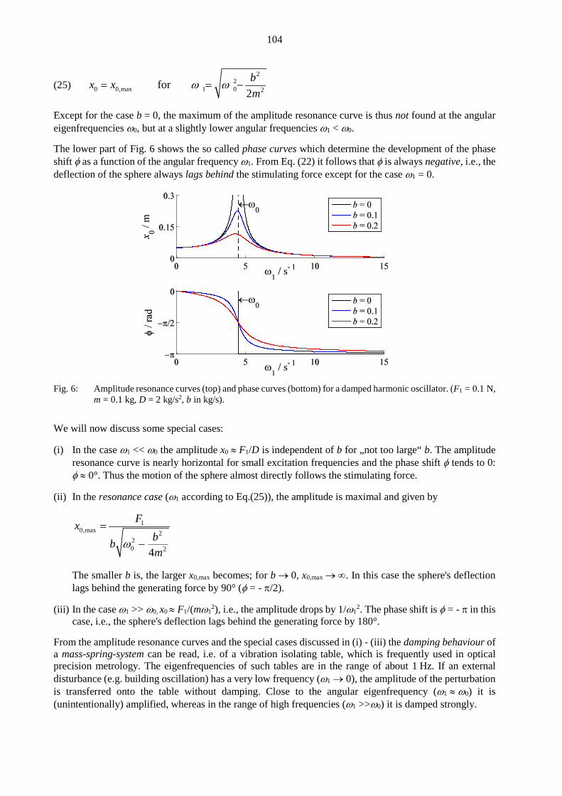
104

(25) 2

20 0,max 1 0 2for

2bx xm

ω ω= = −

Except for the case b = 0, the maximum of the amplitude resonance curve is thus not found at the angular eigenfrequencies ω0, but at a slightly lower angular frequencies ω1 < ω0. The lower part of Fig. 6 shows the so called phase curves which determine the development of the phase shift φ as a function of the angular frequency ω1. From Eq. (22) it follows that φ is always negative, i.e., the deflection of the sphere always lags behind the stimulating force except for the case ω1 = 0.

Fig. 6: Amplitude resonance curves (top) and phase curves (bottom) for a damped harmonic oscillator. (F1 = 0.1 N,

m = 0.1 kg, D = 2 kg/s2, b in kg/s). We will now discuss some special cases: (i) In the case ω1 << ω0 the amplitude x0 ≈ F1/D is independent of b for „not too large“ b. The amplitude

resonance curve is nearly horizontal for small excitation frequencies and the phase shift φ tends to 0: φ ≈ 0°. Thus the motion of the sphere almost directly follows the stimulating force.

(ii) In the resonance case (ω1 according to Eq.(25)), the amplitude is maximal and given by

10,max 2

20 24

Fxbbm

ω=

−

The smaller b is, the larger x0,max becomes; for b → 0, x0,max → ∞. In this case the sphere's deflection

lags behind the generating force by 90° (φ = - π/2).

(iii) In the case ω1 >> ω0, x0 ≈ F1/(mω12), i.e., the amplitude drops by 1/ω1

2. The phase shift is φ = - π in this case, i.e., the sphere's deflection lags behind the generating force by 180°.

From the amplitude resonance curves and the special cases discussed in (i) - (iii) the damping behaviour of a mass-spring-system can be read, i.e. of a vibration isolating table, which is frequently used in optical precision metrology. The eigenfrequencies of such tables are in the range of about 1 Hz. If an external disturbance (e.g. building oscillation) has a very low frequency (ω1 → 0), the amplitude of the perturbation is transferred onto the table without damping. Close to the angular eigenfrequency (ω1 ≈ ω0) it is (unintentionally) amplified, whereas in the range of high frequencies (ω1 >>ω0) it is damped strongly.

105

Fig. 7: Amplitude resonance curves for different masses m (in kg) with other parameters remaining unchanged

(F = 0.1 N, D = 2 kg/s2, b = 0.1 kg/s). The damping behaviour of such a system can be influenced by changing the mass m. Fig. 7 shows that a larger m reduces the angular eigenfrequency with the other parameters remaining unchanged and that the damping for frequencies above the angular eigenfrequency can be increased significantly. Thus, oscillation dampening tables often have large masses in the range of 103 kg. Finally we will examine at which frequency the maximal energy transfer occurs from the generating system to the oscillating system. As we know that the maximal kinetic energy is equivalent to the maximum velocity, we first calculate the temporal course of the velocity v of the sphere using Eq. (20):

(26) ( ) ( )1 0 1 0 1d cos : cosd

xv x t v tt

ω ω φ ω φ= = + = +

With Eq. (24) we thus obtain for the velocity v0:

(27)

( )

1 000 1 0 2

2 12 21 0

x Dv x

bm

m

ωω

ωω ω

= =

− +

and hence:

(28) 000 2

21

1

x DvDm bωω

=

− +

v0 becomes maximal when the denominator of Eq. (28) becomes minimal, i.e., if the following is true (for b ≠ 0):

(29) 1 0 0,max1

0 =Dm v vωω

− = →

Hence it follows:

(30) 1 0 0 0,maxD v vm

ω ω= = → =

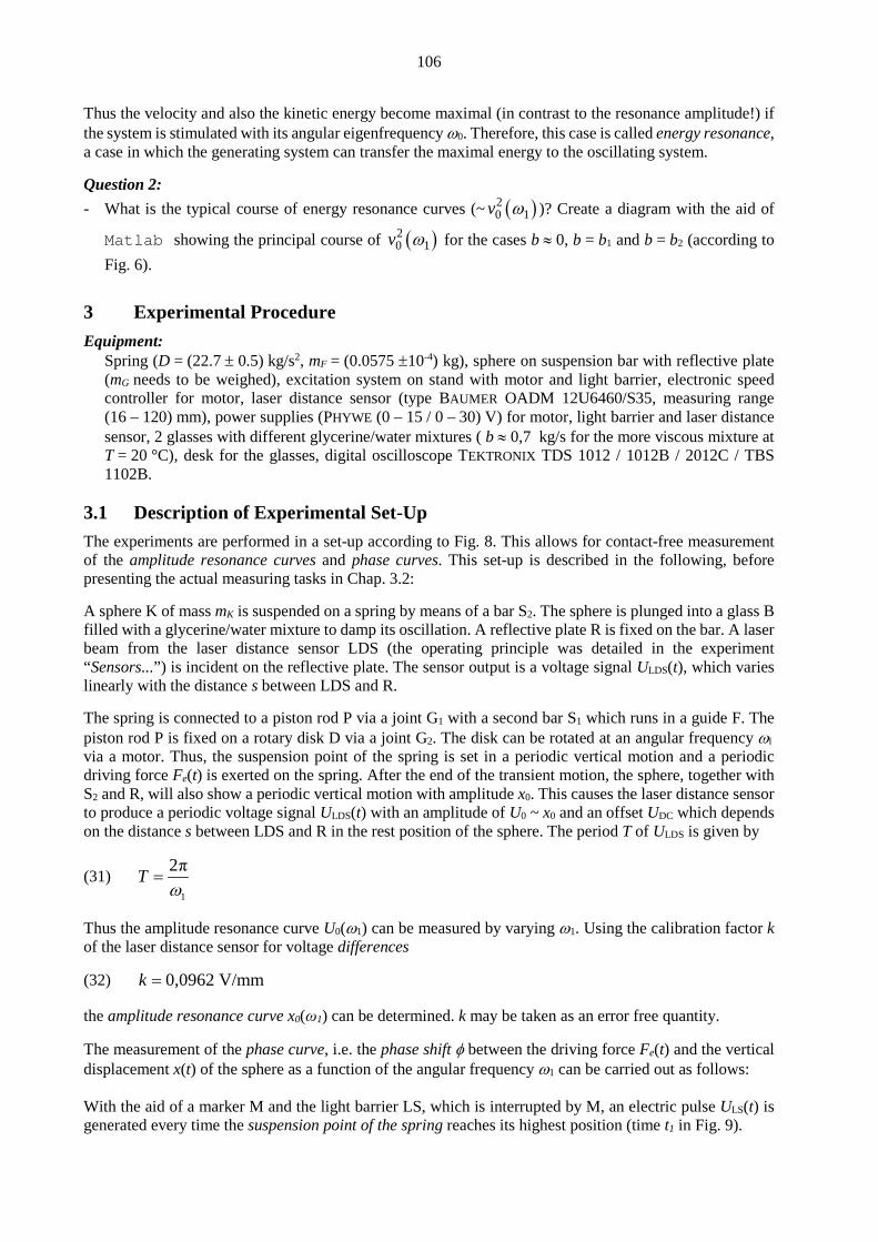
106

Thus the velocity and also the kinetic energy become maximal (in contrast to the resonance amplitude!) if the system is stimulated with its angular eigenfrequency ω0. Therefore, this case is called energy resonance, a case in which the generating system can transfer the maximal energy to the oscillating system. Question 2: - What is the typical course of energy resonance curves (~ ( )2

0 1v ω )? Create a diagram with the aid of

Matlab showing the principal course of ( )20 1v ω for the cases b ≈ 0, b = b1 and b = b2 (according to

Fig. 6).

3 Experimental Procedure Equipment:

Spring (D = (22.7 ± 0.5) kg/s2, mF = (0.0575 ±10-4) kg), sphere on suspension bar with reflective plate (mG needs to be weighed), excitation system on stand with motor and light barrier, electronic speed controller for motor, laser distance sensor (type BAUMER OADM 12U6460/S35, measuring range (16 – 120) mm), power supplies (PHYWE (0 – 15 / 0 – 30) V) for motor, light barrier and laser distance sensor, 2 glasses with different glycerine/water mixtures ( b ≈ 0,7 kg/s for the more viscous mixture at T = 20 °C), desk for the glasses, digital oscilloscope TEKTRONIX TDS 1012 / 1012B / 2012C / TBS 1102B.

3.1 Description of Experimental Set-Up The experiments are performed in a set-up according to Fig. 8. This allows for contact-free measurement of the amplitude resonance curves and phase curves. This set-up is described in the following, before presenting the actual measuring tasks in Chap. 3.2: A sphere K of mass mK is suspended on a spring by means of a bar S2. The sphere is plunged into a glass B filled with a glycerine/water mixture to damp its oscillation. A reflective plate R is fixed on the bar. A laser beam from the laser distance sensor LDS (the operating principle was detailed in the experiment “Sensors...”) is incident on the reflective plate. The sensor output is a voltage signal ULDS(t), which varies linearly with the distance s between LDS and R. The spring is connected to a piston rod P via a joint G1 with a second bar S1 which runs in a guide F. The piston rod P is fixed on a rotary disk D via a joint G2. The disk can be rotated at an angular frequency ω1 via a motor. Thus, the suspension point of the spring is set in a periodic vertical motion and a periodic driving force Fe(t) is exerted on the spring. After the end of the transient motion, the sphere, together with S2 and R, will also show a periodic vertical motion with amplitude x0. This causes the laser distance sensor to produce a periodic voltage signal ULDS(t) with an amplitude of U0 ~ x0 and an offset UDC which depends on the distance s between LDS and R in the rest position of the sphere. The period T of ULDS is given by

(31) 1

2πTω

=

Thus the amplitude resonance curve U0(ω1) can be measured by varying ω1. Using the calibration factor k of the laser distance sensor for voltage differences (32) 0,0962 V/mmk = the amplitude resonance curve x0(ω1) can be determined. k may be taken as an error free quantity. The measurement of the phase curve, i.e. the phase shift φ between the driving force Fe(t) and the vertical displacement x(t) of the sphere as a function of the angular frequency ω1 can be carried out as follows: With the aid of a marker M and the light barrier LS, which is interrupted by M, an electric pulse ULS(t) is generated every time the suspension point of the spring reaches its highest position (time t1 in Fig. 9).

107

Fig. 8: Sketch of the experimental set-up.

Fig. 9: Temporal course of the output voltages of the light barrier LS (ULS) and the laser distance sensor LDS

(ULDS).Time t1: suspension point of the spring at highest position, driving force Fe(t) minimal. Time t2: Sphere at highest position, x(t) and ULDS minimal.

At this time, the driving force Fe(t) = md2x/dt2 is at its minimum (keep in mind the sign according to Fig. 5). At a later time t2, the sphere (not the suspension point of the spring!) reaches its highest position and thus the deflection x(t) its minimum (- x0; here too keep in mind the sign according to Fig. 5). In this posi-tion, the distance s between LDS and R and thus also ULDS(t) is minimal. The phase shift φ between Fe(t) and x(t) is then given by (cf. Fig. 9):

(33) 2 112 : 2

t t t tT T

φ π π ω− ∆

= − = − = − ∆

Therefore by variation of ω1, the phase curveφ (ω1) can be measured. In practice, the amplitude U0(ω1) and time difference ∆t(ω1) are measured simultaneously for each angular frequency ω1 with the aid of an oscilloscope.

P

K

S

Feder

D

1

B

1ω

S2

M

LS

LDS

R

F

G1

G2

s

TU

t

ULS

2t1t

ULDS

108

Finally one remark on the temporal course of the driving force Fe(t): Except a constant phase shift, it cor-responds to the temporal course of the vertical motion of the join G1, i.e. the suspension point of the spring. This motion is described by the quantity y(t) (cf. Fig. 10).

Fig. 10: Definition of quantities for calculating the movement of the join G1 (cf. Fig. 8).

If the piston rod is mounted on the disk at a distance r from the axis of rotation, we obtain: (34) cos cosy r lθ ψ= + and

(35) sin sin sin sinrr ll

θ ψ ψ θ= → =

With

(36) 2

2 22cos 1 sin 1 sinr

lψ ψ θ= − = −

and

(37) 1 tθ ω= we finally obtain:

(38) ( ) ( )2 2 21 1cos siny r t l r tω ω= + −

The purely harmonic motion (r cos(ω1t)) is thus superimposed by a disturbance (square root term in Eq. (38)) which, unfortunately, is also time-dependent and therefore makes the motion anharmonic. Therefore, the driving force Fe(t) is not completely harmonic either. If we choose l >> r, however, l2 >> r2sin2(ω1t) and hence √(...) ≈ l. Instead of a time-dependent disturbance we then have to deal with a merely additive constant l which no longer disturbs the „harmony“.

3.2 Amplitude Resonance Curve and Phase Curve for Strong and Weak Damping Using the setup according to Fig. 8, for a sphere with suspension bar S and reflective plate Rand a spring with known D and mF (for data see Equipment) the amplitude resonance curve x0(ω1) and the phase curve φ(ω1) within the frequency range f1 = ω 1/2π between 0 Hz and approx. 5 Hz are to be measured for two different dampings (glasses containing different glycerine/water mixtures). The piston rod P of the excitation system is fixed to the disk in the second hole from the centre. The anharmonic disturbance according to Eq. (38) can be neglected in this case.

1S

ψ

θ D

1ω

yl

r

G1

109

The output signals of the light barrier (ULS) and the laser distance sensor (ULDS) are displayed on a digital oscilloscope, which is triggered by the signal ULS. The period time T of ULS and the peak-peak value (USS = 2 U0) of ULDS are determined by using the oscilloscope’s MESSUNG / MEASURE function. From these quantities, the angular frequency ω1and the amplitudes U0 and, respectively x0 can be determined. The time difference ∆t = t2 – t1, from which the phase shift φ can be calculated according to Eq. (33) is measured by using the TIME-CURSOR (cf. Fig. 9). Hint:

In order to achieve a mostly uniform motion of the disk, the disk must always be rotated counter clockwise. For the same reason, an electronic speed controller (operating voltage 12 V) must be used for adjusting the revolution number of the motor within the frequency range between 0 Hz and approx. 1.5 Hz, which is mounted between the power supply and the motor. For frequencies exceeding 1.5 Hz the motor can be directly connected with the power supply and the number of revolutions can be con-trolled via the operating voltage (increase voltage slowly from 0 V to max. 12 V).

For both glycerine/water mixtures , the amplitude U0(ω1) of the sphere motion, the period duration T, and the time difference ∆t are measured for as many different values of ω1 as possible (at least 20), especially near the eigenfrequency. The measurements are performed after the end of the transient motion. For the case ω 1 → 0, the amplitude U0 is determined by manually turning the axis of the motor (while the motor is switched off) to the positions “piston rod up”, “piston rod down“ and measuring the corresponding voltages ULDS. We plot x0 over ω1 for both mixtures in one diagram, and φ over ω1 likewise in one diagram. The maximum errors of x0 and φ are also entered in the form of error bars (estimate errors from the fluctuations of the measurements for USS and T at the oscilloscope). Then freehand regression curves are drawn through the measured values and their course is compared with the theoretical expectations. Remarks:

In the vicinity of the angular eigenfrequency the measurement under weak damping may become dif-ficult, because the amplitudes may be large and the spring (possibly even the mount) may get into uncontrollable motion or the sphere may even hit the bottom of the glass. In that case the spring system must be damped manually and rapidly proceeded to the next frequency value.

4 Appendix: Calculation of the Resonance Amplitude and the Phase Shift We want to demonstrate that the resonance amplitude x0 and the phase shift φ can be calculated with a few simple calculation steps, if we change over to complex representation. In complex representation Eq. (19) reads:

(39) 12

12

d d 1 ed d

i tx b x D x Ft m t m m

ω+ + =

In analogy to Eq. (20) we choose as a complex approach:

(40) ( )1 10 0 e ei t i t ix x e xω φ ω φ+= =

Following differentiation and division by 1i te ω insertion of Eq. (40) into Eq. (39) yields:

(41) 2 11 0 1 0 0e e ei i ib D Fx i x x

m m mφ φ φω ω− + + =

Hence it follows with the definition of the angular eigenfrequency ω 0 according to Eq. (8):

110

(42) 1

02 20 1 1

e :i

Fmx zbi

m

φ

ω ω ω= =

− +

As already demonstrated in the experiment “measurement of capacities...”, Eq. (42) is one representation form of a complex number z, whose absolute value (modulus) |z| = x 0 is given by *zz , with z* being the conjugate complex quantity of z. Hence it follows:

(43) 1 1

02 2 2 20 1 1 0 1 1

F Fm mx zz b bi i

m mω ω ω ω ω ω

∗

= = − + − −

from which we obtain Eq. (21) by simple multiplication. For calculating the phase angle we again use (cf. experiment “measurement of capacities...”) the second representation of complex numbers, namely z = α + iβ, α being the real part and β the imaginary part of z. As is generally known, the phase angle φ can be calculated from these quantities as

(44) π for < 0 and 0

arctanπ for < 0 and 0

α ββφα βα

+ ≥ = − <

In order to convert Eq. (42) into the form α + iβ, we extend the fraction in Eq. (42) with the conjugated complex denominator:

(45) ( )

( )

2 21 2 21 10 1 1 0 1 1

0 22 2 2 2 2 12 20 1 1 0 1 1 0 1

ei

F b F F bi im m m m mxb b bi im m m

φω ω ω ω ω ω

ωω ω ω ω ω ω ω ω

− − − − = =

− + − − − +

from which we can read off the quantities α and β :

(46) ( )

( ) ( )

2 21 10 1 1

2 22 21 12 2 2 2

0 1 0 1

and

F F bm m m

b bm m

ω ω ωα β

ω ωω ω ω ω

−= = −

− + − +

which yields by insertion into Eq. (44):

(47) 1

1 02 20 1

arctan

bm

ω

φ π ω ωω ω

= − − ⇔ > −

With

(48) ( ) 1arctan arctan2

yy

π − = −

it finally yields Eq. (22).

111

Carl von Ossietzky University Oldenburg – Faculty V - Institute of Physics Module Introductory laboratory course physics – Part I

Fourier Analysis Keywords:

FOURIER series (trigonometric series), FOURIER coefficients, FOURIER analysis (harmonic expansion, harmonic analysis), amplitude spectrum, phase spectrum, linear system, transfer function, fundamental and harmonics, EULER’s formulas, sampling theorem

Measuring program: Aliasing at violation of the sampling theorem, spectra of photo detector signals, spectra of sound signals, spectrum of a beat signal and an amplitude modulated signal, spectra of a rectangular, a sawtooth, and a triangle signal, GIBBs phenomenon.

References: /1/ HÄNSEL, H., NEUMANN, W.: „Physik – Mechanik und Wärmelehre“, Spektrum Akademischer Verlag,

Heidelberg among others /2/ BRACEWELL, R. N.: „The Fourier Transform and its Applications”, McGraw – Hill, London among others

(advanced) /3/ EICHLER, H.J., KRONFELDT, H.-D., SAHM, J.: „Das Neue Physikalische Grundpraktikum”, Springer-Verlag,

Berlin among others

1 Introduction FOURIER analysis (after JEAN BAPTISTE JOSEPH DE FOURIER, Fig. 1) is an important tool in the area of signal analysis and processing. With its help, it can be determined which harmonic signals1 – with different amplitudes, frequencies, and phases – a periodic signal consists of. In the following, we will limit ourselves to the analysis of time signals. These are signals, for example, like a voltage U(t) or a current I(t) which change in time t. Formally, physical values that change with location can be considered too, like the intensity I(x) of light along the spatial coordinate x.

Fig. 1: Jean Baptiste Joseph de Fourier (1768-1830)2.

We want to cite as an example of the application of FOURIER analysis its importance in system theory for the description of the behaviour of linear systems. The theory of linear systems has a great practical importance in physics. With it, the behaviour of many physical systems can be described without having to know how these systems are internally constructed in detail. We treat these systems as „black boxes” with unknown contents, from which we know that a certain input signal e(t) will result in a certain output signal E(t): Input Output e(t) → linear system → E(t) Linear systems fulfil the condition of linearity (hence the name): A sum of input signals lead to a cor-responding sum of output signals: 1 Harmonic signals means sinusoidal signals in this text. 2 Source: GELLERT, W. et al. [Eds.]: „Kleine Enzyklopädie Mathematik“, VEB Bibliographisches Institut, Leipzig, 1969

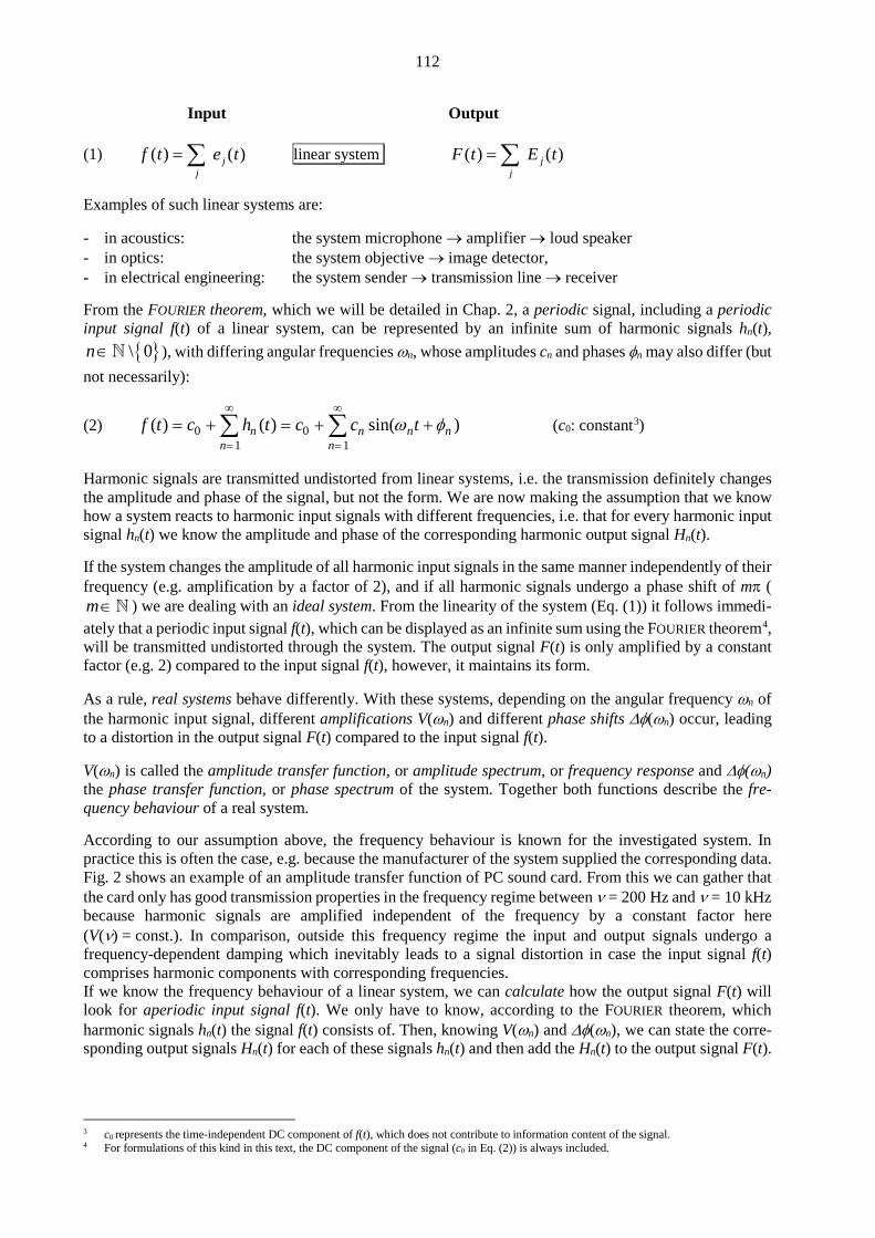
112

Input Output

(1) ( ) ( )jj

f t e t= ∑ linear system ( ) ( )jj

F t E t= ∑

Examples of such linear systems are: - in acoustics: the system microphone → amplifier → loud speaker - in optics: the system objective → image detector, - in electrical engineering: the system sender → transmission line → receiver From the FOURIER theorem, which we will be detailed in Chap. 2, a periodic signal, including a periodic input signal f(t) of a linear system, can be represented by an infinite sum of harmonic signals hn(t),

\ 0n∈ ), with differing angular frequencies ωn, whose amplitudes cn and phases φn may also differ (but not necessarily):

(2) 0 01 1

( ) ( ) sin( )n n n nn n

f t c h t c c tω φ∞ ∞

= == + = + +∑ ∑ (c0: constant3)

Harmonic signals are transmitted undistorted from linear systems, i.e. the transmission definitely changes the amplitude and phase of the signal, but not the form. We are now making the assumption that we know how a system reacts to harmonic input signals with different frequencies, i.e. that for every harmonic input signal hn(t) we know the amplitude and phase of the corresponding harmonic output signal Hn(t). If the system changes the amplitude of all harmonic input signals in the same manner independently of their frequency (e.g. amplification by a factor of 2), and if all harmonic signals undergo a phase shift of mπ (m∈ ) we are dealing with an ideal system. From the linearity of the system (Eq. (1)) it follows immedi-ately that a periodic input signal f(t), which can be displayed as an infinite sum using the FOURIER theorem4, will be transmitted undistorted through the system. The output signal F(t) is only amplified by a constant factor (e.g. 2) compared to the input signal f(t), however, it maintains its form. As a rule, real systems behave differently. With these systems, depending on the angular frequency ωn of the harmonic input signal, different amplifications V(ωn) and different phase shifts ∆φ(ωn) occur, leading to a distortion in the output signal F(t) compared to the input signal f(t). V(ωn) is called the amplitude transfer function, or amplitude spectrum, or frequency response and ∆φ(ωn) the phase transfer function, or phase spectrum of the system. Together both functions describe the fre-quency behaviour of a real system. According to our assumption above, the frequency behaviour is known for the investigated system. In practice this is often the case, e.g. because the manufacturer of the system supplied the corresponding data. Fig. 2 shows an example of an amplitude transfer function of PC sound card. From this we can gather that the card only has good transmission properties in the frequency regime between ν = 200 Hz and ν = 10 kHz because harmonic signals are amplified independent of the frequency by a constant factor here (V(ν) = const.). In comparison, outside this frequency regime the input and output signals undergo a frequency-dependent damping which inevitably leads to a signal distortion in case the input signal f(t) comprises harmonic components with corresponding frequencies. If we know the frequency behaviour of a linear system, we can calculate how the output signal F(t) will look for aperiodic input signal f(t). We only have to know, according to the FOURIER theorem, which harmonic signals hn(t) the signal f(t) consists of. Then, knowing V(ωn) and ∆φ(ωn), we can state the corre-sponding output signals Hn(t) for each of these signals hn(t) and then add the Hn(t) to the output signal F(t).

3 c0 represents the time-independent DC component of f(t), which does not contribute to information content of the signal. 4 For formulations of this kind in this text, the DC component of the signal (c0 in Eq. (2)) is always included.

113

The necessary calculation of the parameters (amplitude, phase, frequency) of the harmonic signals which a periodic signal consists of is called FOURIER analysis or harmonic analysis or harmonic expansion and is the subject of this experiment.

Fig. 2: Amplitude transfer functions of a PC sound card (YAKUMO sound card 16 MCD).

Blue curve: playback, red curve: recording.5

2 Theory In the following section, we are going to omit mathematical proofs which can be looked up in the given literature, and concentrate on the interpretation of the relationships necessary for the experiment.

2.1 Fourier Series and Fourier Coefficients As already mentioned in the introduction, following the FOURIER theorem, a periodic signal f(t) with period T can be represented by a DC component and an infinite sum of harmonic signals whose angular frequencies are integral multiples of ωo = 2π/T. Harmonic signals with angular frequencies

(3) 0 : ; \ 0nn nω ω= ∈ are called harmonics of the fundamental with the fundamental angular frequency ωo, and the sum is denoted as a trigonometric series or a FOURIER series. It is given by:

(4) ( ) ( )0 0 01

( ) cos sinn nn

f t c a n t b n tω ω∞

=

= + + ∑

The values co, an = a(nωo) and bn = b(nωo) are called FOURIER constants or FOURIER coefficients. Deter-mining these values is the subject of the FOURIER analysis. After a short calculation, it is found (cf. e.g. /1/) that they can be obtained from the signal f(t) as follows:

(5) ( )2

0

2

1T

Tc f t dt

T−

= ∫

(6) ( )2

0

2

2 ( )cos 1, 2, 3, ...

T

nT

a f t n t dt nT

ω−

= =∫

5 The gain of an amplifier is often specified using the logarithmic decibel (dB) scale. This is detailed further in the experiment “Operational

amplifier“ in the SuSe. An amplification by x dB corresponds to a linear amplification by the factor 10x/20.

10

0

-10

10

0

-1020 50 100 200 500 1k 2k 5k 10k 20k

ν / Hz

V / dB

114

(7) ( )2

0

2

2 ( )sin 1, 2, 3, ...

T

nT

b f t n t dt nT

ω−

= =∫

The constant c0 is the average (DC component) of the signal f(t). If, e.g., f(t) is a temporally oscillating voltage U(t), c0 corresponds to the DC voltage of the signal. The representation of the FOURIER series in Eq. (4) can be simplified if the following relationship is used:

(8) ( ) ( )0 0 0cos sin sin( )n n n na n t b n t c n tω ω ω φ+ = + with

(9) 2 2n n nc a b= +

and

(10) arctan nn

n

ab

φ

=

With this, Eq. (4) becomes the spectral form of the FOURIER series:

(11) 0 01

( ) sin( )n nn

f t c c n tω φ∞

=

= + +∑

A periodic signal f(t) can be described after FOURIER analysis with the following values6 (12) c0 : DC component (average of the signal f(t), cf. Eq. (5)) cn = cn(nω0) : amplitude spectrum φn = φn(nω0) : phase spectrum

Fig. 3: Top (red): Anharmonic but periodic signal f(t) with period T = 1 (in arbitrary units) with its harmonic

components h1(t) (middle, blue) und h2(t) (bottom, blue).

6 The graphic representation of cn over ωn is called amplitude spectrum. The graphic representation of an over ωn is called cosine spectrum; the

representation of bn over ωn is called sine spectrum.

115

Two examples will make the relations clear. The first example shows a quite simple case. In Fig. 3 an anharmonic, but periodic, signal f(t) = h1(t) + h2(t) with period T = 1 (in arbitrary units) is shown at the bottom. It is composed of the two harmonic signals shown beneath it in the figure: the fundamental h1(t) with the amplitude c1 = 0.5 (in arbitrary units), the angular frequency ω1 = 1×ω0 = 2π/T, and the phase φ1 = π and the first harmonic h2(t) with the same amplitude c2 = 0.5, the angular frequency ω2 = 2×ω0, and the phase φ2 = π/2. A FOURIER analysis of the signal f(t) would then produce: DC component: c0 = 0 amplitude spectrum: c1 = c1(ω0) = 0.5

c2 = c2(2ω0) = 0.5 cm = cm(mω0) = 0 ∀ m ≥ 3 phase spectrum: φ1 = φ1(ω0) = π φ2 = φ2(2ω0) = π/2 φm = φm(mω0) = 0 ∀ m ≥ 3 The amplitude and phase spectra, that is cn(ωn) and φn(ωn), are represented in Fig. 4.

Fig. 4: Amplitude spectrum (left) and phase spectrum (right) of the signal shown at the top in Fig. 3. Generally,

vertical spectral lines from the abscissa to the respective ordinate value are drawn instead of data points in such diagrams.

Fig. 5: Anharmonic, periodic signal f(t) (upper left, red) with its five harmonic components (upper right as well as

middle and below, blue). Abscissa: t, ordinate: f(t) or hn(t), respectively, period T = 1 (t and f(t) in arbitrary units).

ω0 2ω ωn3ω 4ω

cn

0 0 0 ω0 2ω ωn3ω 4ω

φnπ

0 0 0

π/20,5

116

Clearly the situation shown in Fig. 5 is more complex: in the upper left diagram an anharmonic, but peri-odic, signal f(t) with period T = 1 (in arbitrary units) is shown. To its right the fundamental is shown with angular frequency ω1 = 1×ω0 = 2π/T and underneath four harmonics with the angular frequencies ωn = nωo, n = 2, 3, 4, 5 which all have different amplitudes and phases. A FOURIER analysis would lead to the DC component of c0 = 0 as well as five values of cn for the amplitude spectrum and five values of φn for the phase spectrum. Question 1: - Try graphically to get the data necessary from Fig. 5 to sketch the amplitude and phase spectra analo-

gously to Fig. 4. Control with the help of Matlab, whether your analysis is right.

2.2 Sampling and Sampling Theorem We now know how the FOURIER coefficients a0 , an and bn can be calculated, and from there, the values c0, cn and φn, i.e., the amplitude and phase spectra of periodic signals f(t). In practise, a problem appears here: The signals under investigation are, in general, not analytically known signals , but rather measured signals having a complicated temporal course that were recorded by, e.g. a data acquisition board connected to a computer. Such recording systems yield discrete function values yi = f(ti)7 at equidistant time points ti (separation of ∆t). It is also said that the signal f(t) is sampled at the points ti with sampling angular frequency ωa = 2π/∆t. The FOURIER analysis of a sampled signal is of course only an approximation – since the signal itself is only known approximately (i.e. only at the points ti). How a FOURIER analysis is carried out in such a case is shown in the following. Let us assume that from the signal f(t) we have 2m measured points (sampling points) yi= (i = 1,…,2m-1) at equidistant time points ti. For the FOURIER coefficients we then get:

(13) 2 1

00

12

m

ii

c ym

−

== ∑

(14) 2 1

0

1 2πcos2

m

n ii

n ia ym m

−

=

=

∑ n = 1, 2,..., m

(15) 2 1

0

1 2πsin2

m

n ii

n ib ym m

−

=

=

∑ n = 1, 2, ..., m-1

From 2m independent function values we get m coefficients an, (m - 1) coefficients bn, and a constant c0. Together that is m + (m - 1) + 1 = 2m independent FOURIER coefficients. This is understandable from the point of view of the information content: the information content cannot be lost or increased through simple calculation. The sampling theorem (SHANNON theorem8), with the help of Eqs. (13) – (15), answers the question of the least number of function values that are needed to reliably determine the angular frequency ωs of a harmonic oscillation present in a signal f(t). It says that an angular frequency ωs can be reliably detected if the following holds for the sampling angular frequency ωa: (16) 2a sω ω> sampling theorem In other words: The angular frequency ωs of a harmonic signal can only be reliably determined, if more than two sampling values per period are available for the signal. If the condition given by the inequality (16) is violated, the signal with angular frequency ωs is „under sampled” which leads to false results (alias-ing effects). In this case, the FOURIER analysis produces the wrong angular frequency ωf. 7 Compare experiment “Data Acquisition with the PC ...“. 8 CLAUDE ELWOOD SHANNON (1916 - 2001).

117

(17) f a sω ω ω= − The signal with the angular frequency ωs hence shows up in the amplitude spectrum under the ”wrong name” ωf, and therefore the term „alias”. For ωs ≤ ωa ≤ 2ωs, it appears in the spectrum reflected at the axis ω = ωa/2. If the sampling angular frequency ωa is given, a harmonic signal can, according to Eq. (16), only be sampled correctly, if

(18) 2a

sωω <

is true for its angular frequency ωs. The angular frequency ωa/2 is also called NYQUIST frequency9. If the sampling theorem is met, the length 2 m ∆t of the time interval over which the measured signal was sampled determines the frequency resolution ∆f, i.e. the accuracy with which signal frequencies can be measured:

(19) 1~

2f

m t∆

∆ This aspect of the FOURIER analysis, however, cannot be discussed further in the introductory laboratory course.

2.3 Practical Hints The calculations of the FOURIER coefficients, rather of the amplitude and phase spectra, are quite extensive. Today, however, they can be done very quickly with a personal computer, and in the case of large data sets the use of special processors can accelerate the calculations. It was not so long ago that the intensive work had to be done by hand. In a mathematic handbook from the year 1969 the following tip is given (GELLERT, W. et al. [Eds.]: „Kleine Enzyklopädie Mathematik”, VEB Bibliographisches Institut, Leipzig, 1969):

„A person practised in calculating, who is using an electronic calculation machine and applying a special method of calculation for harmonic analysis, needs about ½ an hour for 12 points, about 2 hours for 24 points, about 6 hours for 36 points, and about 16 hours for 72 points … A medium speed electronic calculation machine manages the calculation of 36 points in about 2 minutes. The time needed to print the results is usually longer than the calculation time.”

In the following investigation the FOURIER analysis will be performed with a few hundred to a few thousand points. Either don’t make any plans for your semester break – or use the PC at your disposal and you will be finished without problems in one afternoon! In practise, one is only interested in finding out which amplitude the harmonic signals have that are con-tained in a periodic measured signal. The phase of the single components is often unimportant. In other words: the amplitude spectrum is, in most cases, of considerably more practical importance than the phase spectrum. With the present investigation we will thus limit ourselves to the interpretation of the amplitude spectra. For a non–periodic signal f(t) defined in a time-interval of length τ (e.g. an output pulse from a fotodiode), the signal can be thought of as continuing periodically to the right and to the left of the given interval (with the „period” τ), and it can likewise be represented by a FOURIER series. It is the case that such a FOURIER series produces function values according to Eq. (4) which are situated outside of the definition interval τ, however, these values may simply be ignored for further considerations.

9 HARRY NYQUIST (1889 - 1976).

118

3 Experimental Procedure Equipment:

Digital oscilloscope TEKTRONIX TDS 1012 / 1012B / 2012C / TBS 1102B, PC with data acquisition board (NATIONAL INSTRUMENTS 6014 PCI or 6221 PCI) and accompanying BNC adapter (NATIONAL INSTRUMENTS BNC-2120), 2 function generators (TOELLNER 7401 and AGILENT 33120A / 33220A), addition amplifier, photo diode with integrated amplifier and pinhole diaphragm (diameter 1mm), AC filter for photo diode, incandescent lamp and fluorescent lamp in light-proof box, microphone with preamplifier, tuning fork, power supply (PHYWE (0 - 15 / 0 - 30) V).

3.1 General Hints

3.1.1 Operating the Data Acquisition Board The input selection switch on the connector board of the data acquisition board has to be set to „FS” (Floating Source). The connection of the signal sources (function generator, microphone amplifier etc.) in principle only works with the BNC socket of the input channel 0 (ACH 0 or AI 0); the switch above the BNC socket of ACH 0 or AI 0 has to be set to BNC.

3.1.2 Input Voltage Range of the Data Acquisition Board The maximum input voltage range that the data acquisition board can withstand is ± 10 V; this should not be exceeded. As a control, all of the input signals of the data acquisition board are therefore simultaneously displayed on the oscilloscope.

3.1.3 Software The following experiments are performed using theMATLAB-Scripts „Fourieranalyse.m” and „Rekonstruktion.m”, respectively (available under Q:). The scripts announce themselves by self–explanatory screen messages. Text messages of the scripts such as tables with amplitudes and frequencies of FOURIER components appear in the Command Window. There, they can be marked and transferred to other applications by „Copy and Paste” (e.g. Word,Notepad-Editor among others).

3.1.4 Printing and Saving the Graphics The graphics (Matlab figures) can be sent to the printer in the lab using the key combination → File → Print. Via → File → Save as they can be stored in various well known graphics formats. Details of graphics can be magnified by using the Zoom function in the Figure window.

3.2 Sampling Theorem With the help of the AGILENT-function generator a sinusoidal time signal U(t) without a DC component and with a frequency of 140 Hz and an amplitude of 4 V is generated (control of settings on the oscillo-scope) and fed into the ACH 0 or AI 0 input of the data acquisition board. With the program Fourieranalyse 1,000 sampling values for each sampling frequency of (1000, 500, 300, 200, 150, 120) Hz should be read and FOURIER analysed. The results (time signals and amplitude spectra) are printed or stored, respectively. Question 2: - How can the results be interpreted when Eq. (16) to Eq. (18) are taken into consideration?

3.3 Spectra of the Signal of a Photo Detector During the investigation of the oscilloscope we saw that the temporal course of the light intensity of a light bulb connected to the 230 V power supply system looked clearly different than the temporal course of the light intensity of a fluorescent lamp. We now want to quantitatively investigate this qualitative finding. To do this, a photo diode is illuminated by an incandescent lamp connected to the power supply system and then by a fluorescent lamp also connected to the 230 V power supply system. A suitable pinhole in front

119

of the photo diode prevents saturation of the output signal of the photo diode amplifier (time signal U(t)). With the help of the AC filter the DC component of the measured signal is filtered out (control on the oscilloscope), and then the signal is fed into the ACH 0 or AI 0 input channel of the data acquisition board. With the help of the program Fourieranalyse, 5,000 sampling values should be read for both signals at a sampling frequency of 5 kHz and FOURIER analysed. The results (time signals and amplitude spectra) are printed and stored, respectively. Question 3: - What is the difference between the time signals and the difference between their amplitude spectra?

(Statements about the absolute amplitudes of the spectral components are not of importance.)

3.4 Spectra of Sound Waves Recorded with a Microphone Next the fundamental frequency of a tuning fork will be determined. For this, the tuning fork is struck and the sound waves produced are recorded with the help of a microphone by placing the foot end of the tuning fork on top of the microphone. The output from the microphone is amplified with the accompanying amplifier and its output signal U(t)) is fed into the ACH 0 or AI 0 input of the data acquisition board. With the program Fourieranalyse 10,000 sampling values are read at a sampling frequency of 5 kHz and FOURIER analysed. The result (time signal and amplitude spectrum) is printed or stored, respectively. Question 4: - Does the amplitude spectrum correspond with musical expectations? In the second step, the note from the tuning fork (the a’) should be sung and then hummed. For both cases the acoustic signals should be recorded using the microphone and an analysis like that for the tuning fork should follow. Question 5: - What does the result look like in comparison to the analysis of the tuning fork oscillation?

3.5 Spectrum of a Beat Signal With the help of an addition amplifier the sinusoidal signals from two function generators (AGILENT and TOELLNER) are added. One generator is operated at 104 Hz, amplitude 1 V, no DC component, the other at 108 Hz, amplitude 0.75 V, no DC component (verify the settings with the digital oscilloscope). The output signal of the addition amplifier (time signal U(t)) is fed into the ACH 0 or AI 0 input channel of the data acquisition board and observed simultaneously with the oscilloscope. With the program Fourieranalyse 10,000 sampling values are read at a sampling frequency of 2 kHz and FOURIER analysed. The result (time signal and amplitude spectrum) is printed or stored, respectively, and the course of the amplitude spectrum is interpreted.

3.6 Spectrum of an Amplitude-Modulated Signal Let us examine a harmonic voltage signal U(t) of the form

(20) ( ) ( )sinT TU t U tω= with the amplitude UT and the angular frequency ωT. If a time-dependent signal UM(t) is added to the con-stant amplitude UT, then an amplitude-modulated signal is obtained10:

(21) ( ) ( ) ( )sinT M TU t U U t tω= + The signal from Eq. (20) is called carrier signal and ωT is called carrier angular frequency. In the simplest case, UM(t) is a harmonic signal with the angular frequency ωM and the amplitude UM0. Hence, it follows: 10 The principle of amplitude modulation (AM) is used, e.g., for signal transmission in long-, medium- and short-wave broadcast. The current

standard in the ultrashort-wave range is the frequency modulation (FM).

120

(22) ( ) ( ) ( )0 sin sinT M M TU t U U t tω ω= + This equation can be converted to:

(23) ( ) ( ) ( )( ) ( )( )0sin cos cos2M

T T T M T MUU t U t t tω ω ω ω ω = + − − +

Question 6: - Draw the amplitude spectrum of the signal U(t) according to Eq. (23) for the cases UT = 2UM0 = 1 V, ωT/2π = 750 kHz and ωM/2π = 15 kHz.

With the AGILENT function generator an amplitude-modulated signal according to Eq. (22) with the follow-ing parameters is generated: UT = 2 V, ωT/2π = 1 kHz, UM0 = 1 V, ωM/2π = 200 Hz (see footnote11!). The signal (time signal U(t)) is fed into the input channel ACH 0 or AI 0 of the data acquisition board and simultaneously observed with the oscilloscope. Using the program Fourieranalyse 10,000 sampling values are read at a sampling frequency of 10 kHz and FOURIER analysed. The result (time signal and amplitude spectrum) is printed or stored. The course of the amplitude spectrum is compared to the expectations according to Eq. (23).

3.7 Spectrum of a Square Signal, Gibbs Phenomenon The square signal of a function generator (time signal U(t); amplitude 4 V, frequency 50 Hz, no DC com-ponent) is fed into the ACH 0 or AI 0 input channel of the data acquisition board. Using the program Rekonstruktion 10,000 sampling values are read at a sampling frequency of 10 kHz and FOURIER analysed. The result (time signal and amplitude spectrum) is printed or stored and the course of the amplitude spectrum is compared to the theoretical expectations. For this comparison, the expected and measured amplitudes for the ten spectral components with the largest amplitudes are also plotted in tabular form. Hint:

Descriptions of the FOURIER analysis for a square signal are found in almost every physics text book or, for example, in the “Taschenbuch der Mathematik”or in the online reference material from WOLFRAM RESEARCH (cf. http://www.uni-oldenburg.de/en/physics/teaching/laboratory-courses/literature/ ). The measured data required for the comparison are given in the Matlab com-mand window and can be copied into a personal file from there.

Subsequently, the time signal is reconstructed by stepwise addition of its FOURIER components (FOURIER synthesis). Thus, it is clearly shown how the original square signal can be reconstructed piece by piece from its FOURIER components, if more and more harmonics are added to the fundamental during reconstruction. The result of the reconstruction is printed or stored, respectively. Looking at the reconstructed square signal it becomes clear that over- and undershooting occur. This effect is called GIBBS phenomenon12. It occurs whenever the signal shows a discontinuity like the square signal at the transition point from the lower to the upper or from the upper to the lower signal level (cf. Fig. 6). The overshoots themselves are called GIBBS humps. The larger the number N of harmonics, which are used for the synthesis of the square signal, the closer the extrema of the under- and overshoots move together – their amplitudes, however, staying the same for large N. An exact but extensive calculation yields that the largest overshoot has a height of about 9% of the amplitude of the square signal, while the height of the largest undershoot amounts to about 4.8% of the amplitude.

11 These parameters were stored in the internal storage “1“ in the function generator. They can be retrieved by clicking the button RECALL; first,

there appears RECALL 0 with a blinking 0 in the display. By clicking the button the 0 is raised to 1, then click on ENTER. Now, the function generator produces the required signal at the OUTPUT socket.

12 JOSIAH WILLARD GIBBS (1839 - 1903)

121

Fig. 6: GIBBS phenomenon for the FOURIER synthesis of a square signal with an amplitude of 1 V and a

period of 2 s. Left N = 50, right N = 100.

3.8 Spectra of a Saw Tooth Signal and a Triangle Signal The investigation described in Chap. 3.7 is repeated for a saw tooth signal and then for a triangle signal (amplitude of the signals always 4 V, frequency 50 Hz, no DC component; sampling frequency 10 kHz, 10,000 sampling values). The time signal and the amplitude spectra are printed or stored and the courses of the amplitude spectra are compared to the theoretical predictions. Presentations of the Fourier-analysis of both signals can be found in the references given in Chap. 3.7. Finally, both signals are reconstructed from their spectra. The results of the reconstruction are printed or stored, respectively. Question7: - For which signal is the GIBBS phenomenon noticeable, and how come?

122

Carl von Ossietzky University Oldenburg – Faculty V - Institute of Physics Module Introductory laboratory course physics – Part I

Surface Tension, Minimal Surfaces, and Coffee Stains

Keywords: VAN DER WAALS forces, specific surface energy, surface tension, minimal surfaces, capillarity, contact angle, cohesion, breaking-off method, bubble pressure method

Measuring program: Observation of minimal surfaces, observation of mass transport during the evaporation of a liquid drop, measurement of the surface tension with the breaking-off method and the bubble pressure method, pressure within gas bubbles.

References: /1/ DEMTRÖDER, W.: „Experimentalphysik 1 - Mechanik und Wärme“, Springer-Verlag, Berlin among others /2/ EICHLER, H. J., KRONFELDT, H.-D., SAHM, J.: „Das Neue Physikalische Grundpraktikum“, Springer-Verlag,

Berlin among others. /3/ WALCHER, W.: „Praktikum der Physik“, Teubner Studienbücher, Teubner-Verlag, Stuttgart

1 Introduction Many of you may still remember a childhood experiment: a pin was laid onto a water surface and did not submerge. Or maybe you remember observing insects which are able to run over the water surface of a pond without sinking. Both phenomena are explained by the surface tension of liquids. The following experiment deals with their quantitative measurement.

2 Theory Various interaction forces are effective between the molecules within a liquid, the most important ones being the VAN DER WAALS forces, which originate from electrostatic forces. These interaction forces are effective at very short distances of about 10-9 m and cause the molecules to hold together (cohesive forces). They are considerably stronger than the interaction between the molecules of a liquid and those of gases (adhesive forces) above the surface of the liquid (e.g. air). This leads to the situation represented in Fig. 1: equally strong forces act on the molecules within the liquid in all directions and neutralize one another, the resultant force FR being zero. However, within a thin layer at the surface of the liquid a net force FR ≠ 0 remains directed towards the interior of the liquid, perpendicular to the surface.

Fig. 1: On the origin of the surface tension of liquids; here, at the interface between a liquid and air. FR: resultant

force acting on a liquid molecule. If the surface of a liquid is to be increased by driving liquid molecules from the interior of the liquid to its surface, this force FR has to be overcome; the potential energy of the molecules is increased. From this we can immediately draw an important conclusion: Since a state of equilibrium is characterized by a minimum of potential energy, liquid surfaces cover minimal surfaces without the impact of external forces. Impressive minimal surfaces are easy to demonstrate by dipping differently shaped wire and plastic frames into soapsuds and then removing them. The soap film lamellae formed between the wires or fins represent minimal surfaces.

F ≠ 0R

F = 0R

LuftFlüssigkeit

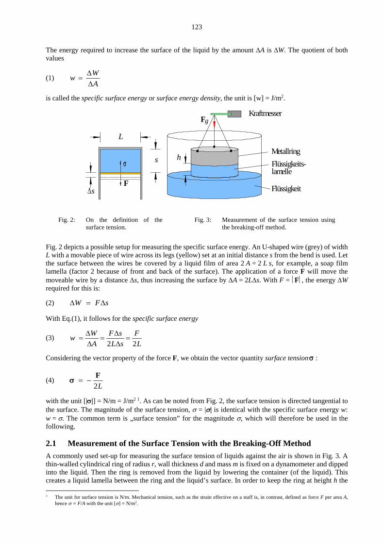
123

The energy required to increase the surface of the liquid by the amount ∆A is ∆W. The quotient of both values

(1) w WA

=∆∆

is called the specific surface energy or surface energy density, the unit is [w] = J/m2.

Fig. 2: On the definition of the surface tension.

Fig. 3: Measurement of the surface tension using the breaking-off method.

Fig. 2 depicts a possible setup for measuring the specific surface energy. An U-shaped wire (grey) of width L with a movable piece of wire across its legs (yellow) set at an initial distance s from the bend is used. Let the surface between the wires be covered by a liquid film of area 2 A = 2 L s, for example, a soap film lamella (factor 2 because of front and back of the surface). The application of a force F will move the moveable wire by a distance ∆s, thus increasing the surface by ∆A = 2L∆s. With F = F, the energy ∆W required for this is: (2) W F s∆ = ∆ With Eq.(1), it follows for the specific surface energy

(3) 2 2

W F s FwA L s L

∆ ∆= = =

∆ ∆

Considering the vector property of the force F, we obtain the vector quantity surface tension σ :

(4) 2L

= −F

σ

with the unit [|σ|] = N/m = J/m2 1. As can be noted from Fig. 2, the surface tension is directed tangential to the surface. The magnitude of the surface tension, σ = |σ| is identical with the specific surface energy w: w = σ. The common term is „surface tension” for the magnitude σ, which will therefore be used in the following.

2.1 Measurement of the Surface Tension with the Breaking-Off Method A commonly used set-up for measuring the surface tension of liquids against the air is shown in Fig. 3. A thin-walled cylindrical ring of radius r, wall thickness d and mass m is fixed on a dynamometer and dipped into the liquid. Then the ring is removed from the liquid by lowering the container (of the liquid). This creates a liquid lamella between the ring and the liquid’s surface. In order to keep the ring at height h the 1 The unit for surface tension is N/m. Mechanical tension, such as the strain effective on a staff is, in contrast, defined as force F per area A,

hence σ = F/A with the unit [σ] = N/m2.

L

s

F

σ

∆ s

MetallringFlüssigkeits-lamelle

Flüssigkeit

h

FKraftmesser

g

124

force F(h) is required. Let us assume that, proceeding from the height h, we can withdraw the ring by an additional small distance ∆h from the liquid to the height h0, such that the lamella just does not cut into itself and finally break off. The required work to achieve this is

(5) ( )0W F h h∆ = ∆ by which the surface is enlarged by: (6) 2 2 πA r h∆ = × ∆ For the surface tension we thus get:

(7) ( ) ( )0 0

2 2 π 4πF h h F hW

A r h rσ

∆∆= = =

∆ × ∆

By means of this breaking-off method it is possible to determine the surface tension σ of liquids against the air by measuring the maximum force F:=F(h0), at which the lamella just does not cut into itself and finally break off, and the ring radius r. It should be noted that the dynamometer indicates the total force Fg

(8) gF F mg= + m being the mass of the ring including suspension and g the gravitational acceleration. Thus, the force F to be inserted into Eq. (7) is:

(9) gF F mg= − That is the theory so far. In practice, the value determined with Eq. (7) has to be multiplied by a correction factor ƒ which we give here without deduction and which we assume to be error-free 2:

(10) 20.36070.725 0.04534 0.839 df

rr gσ

ρ= + + −

where σ is the raw value of the surface tension from Eq. (7) and ρ the density of the liquid. The corrected value σk of the surface tension is:

(11) k fσ σ=

2.2 Measurement of the Surface Tension with the Bubble Pressure Method Another method for measuring the surface tension is presented in Fig. 4. A sharp-tipped capillary K with a small interior radius r is dipped vertically into a liquid (immersion depth h), the surface tension of which is to be measured against the air. The capillary is connected to an apparatus for measuring changes in air pressure that was previously detailed in the experiment “Sensors...”. The air pressure inside the capillary can be measured with the pressure sensor D. In order to press the air to the outlet of the capillary, the hydrostatic counter pressure pF in the liquid must be overcome, it is given by (12) p ghF = ρ ρ being the density of the liquid and g the gravitational acceleration. If the air pressure in K is further increased, air bubbles of radius R slowly form at the outlet of the capillary (Fig. 5), whose inner pressure is reciprocally proportional to R. With increasing pressure, the air is further pressed out of the capillary and the radius R of the bubbles therefore continues to decrease. In the case R = r the radius is minimal and the

2 according to KOSE, V. [Ed..]; WAGNER, S. [Ed.]: “Kohlrausch – Praktische Physik Bd. 1“, Teubner, Stuttgart, 1996

125

pressure in the bubble, which is then hemispherical in shape, is maximum. After exceeding this pressure the bubble grows and finally breaks off from the outlet. The pressure in the capillary collapses and the process of bubble formation starts again.

Fig. 4: Set-up of bubble pressure method used to measure the surface tension. For details, refer to the experiment

“Sensors…”. Let ∆p be the overpressure against the hydrostatic pressure at the capillary outlet at which the pressure in the bubbles is maximal and their radius is r. If ρm is the density of the liquid in the manometer (here water) and hm the height displayed by the manometer, we obtain for ∆p:

(13) ( )m mp h h gρ ρ∆ = − With that the surface tension can be calculated approximately by:

(14) 2

2 112 3 6

r p r g r gp p

ρ ρσ ∆ = − − ∆ ∆

Fig. 5: Air bubbles (grey, radius R) at the outlet of a capillary of radius r dipped into a liquid. The dotted lines

mark the imaginary form of a free bubble of radius R.

Wasser

M

Luft, Druck p

EV

S

hm

Wasser

D

- +pLH

H1

2

B

K

h

2 r

R = rR >> r R > r

Luftzufuhr

R > r

126

Equation (14) represents an approximate solution, the deduction of which is neglected here, because it is not easy to understand. In any case, famous physicists like ERWIN SCHRÖDINGER, one of the founders of quantum mechanics, contributed to that equation! 3 For small capillary radii r, the two last terms in Eq. (14) (correction terms) are of no importance and we can write:

(15) 2

r pσ ∆≈

The advantage of this bubble pressure method over the breaking-off method is the fact that the surface tension is measured at a new surface, namely on the gas bubble in the liquid. Impurity of the liquid surface caused by the ambient air, potentially causing errors when using the breaking-off method, does not matter in this case.

2.3 Physics in Coffee Stains Putting a drop of liquid onto a solid slippery surface, e.g. water on glass, leads to a certain contact angle between the liquid and the surface at incomplete wetting which is determined by the properties of the materials involved, in particular by the surface tension of the liquid. By small defects on the surface the margin of the drop can be fixed at the surface. If the liquid contains a dissolved substance, as e.g. coffee in water, the fixing is caused by the dissolved substance itself, i.e. it also occurs at “perfect” surfaces 4. As a consequence of the fixing of the drop margin, the drop keeps its radius during evaporation of the liquid. Therefore, liquid which evaporates on the edge must be replaced by liquid from the drop’s centre. This leads to a “capillary flow” to the outside (Fig. 6), by which the dissolved substance is permanently trans-ported to the drop’s margin. Therefore, after the drop has dried completely, considerably more coffee is found at the drop’s margin than inside the drop. The light centre of the coffee spot is therefore surrounded by a dark edge.

Fig. 6: Left: Radial capillary flow in a liquid drop on a glass surface5. The flow was made visible by multiple

exposure of small micro spheres (diameter 1 µm), which were added to the liquid. Right: dried coffee stain with higher coffee concentration at its margin caused by such a flow.

3 Experimental Procedure Equipment:

Ring (r = 25,52 mm, d = 0,25 mm, both error-free) with suspension, vertically adjustable platform, force sensor using strain gauge technique (U-OL, measurement range 100 mN), measurement amplifier for force sensor (U-OL), set of weights for calibrating the force sensor, capillary tube (inner diameter d = (2.07 ± 0.01) mm) in suspension at unit for vertical adjustment (reading accuracy 0.02 mm), pressure sensor (SENSORTECHNICS HCLA12X5DB) on base plate with valves on mount, ERLENMEYER flask with smoothed plug on table, U-tube manometer (filled with water) with holder and reading scale,

3 cf. E. SCHRÖDINGER: „Notiz über den Kapillardruck in Gasblasen“, Ann. Phys. 46.4 (1915) 413 - 418. 4 cf. R. D. DEEGAN: „Pattern formation in drying drops“, Phys. Rev. E 61.1 (2000) 475 - 485 5 cf. R. D. DEEGAN: „Capillary flow as the cause of ring stains from dried liquid drops“, Nature 389 (1997) 827 – 829.

127

stand with adjustable pointers, beaker glasses, flexible tubes, tube couplings, taps, scissor jack, thermometer (accuracy 0.1° C), distilled water, soap suds, plastic frames, glass tube stand with two inlets and two outlets, microscope slides, toothpick, Aluminium plate, red wine, ethanol bath, bath with distilled water, hair-drier, nitrogen gas flask, kitchen paper roll, power supply (PHYWE (0 - 15 / 0 - 30) V), PC with data acquisition board (NATIONAL INSTRUMENTS PCI 6014 or PCI 6221) and BNC-Adapter (NATIONAL INSTRUMENTS BNC-2120).

3.1 Minimal Surfaces Sketch your expectations concerning minimal surfaces after dipping and withdrawing the available plastic frames6 from the soapsuds while preparing the experiment. Compare your expectations with the experimen-tally obtained minimal surfaces. Note that local minima may form in addition to the global (absolute) minimum (Fig. 7).

Fig. 7: Global minimum of a target value as a function of a parameter. Besides the global minimum, there are many

local minima one of which has been marked exemplarily.

3.2 Red Wine Stains Pour some drops of red wine on to a microscope slide. Draw the drops into interesting forms with a pipette and observe how the fruit flesh concentration changes by evaporation of the liquid within the drops during the laboratory course. To accelerate the evaporation of the liquid, the slides are put onto a thin Aluminium plate above a radiator.

3.3 Measurement of the Surface Tension Using the Breaking-Off Method The surface tension of distilled water against air is to be measured using an experimental set-up according to Fig. 3. A bending rod is used as force sensor, which is already known from the experiment “Sensors...”. Hints: - The suspension threads of the ring were adjusted by the technical assistant prior to the experiment so

that the ring hangs horizontally. Do not change this adjustment without informing the technical assistant or supervisor!

- The ring must not be touched with bare hands in order to avoid grease and sweat traces which would falsify the measuring results. Therefore, hold the ring with suspension threads only!

First, the force sensor suspended on a stand is calibrated using a set of weights. For at least five weights G in the range of (0 – 100) mN the output voltage UM of the measurement amplifier (Damping / Dämpfung on) is measured. The measurement is carried out by means of a data acquisition board in a PC 7 using the Matlab-script DatenEinlesen.m (available on Q:). This is a more comprehensive and more comfortable version of the script which was used during the experiment „Data Acquisition and Processing with the PC…“. The graphic user interface created by the script is self-explaining. UM is plotted over G = m g and a calibration curve (regression line) is determined by means of linear regression. For g, the value for Oldenburg is used: g = 9.8133 m/s2; it may be taken to be exact (error free)8. 6 Photographs of the plastic frames can be found on the GPR web site. 7 Input switch set to „FS“ (Floating Source). Output of the measurement amplifier connected to the BNC jack of input channel 0 (ACH 0 or AI

0); wiper switch above the BNC jack of ACH 0 or AI 0 set to BNC. 8 Value according to http://www.ptb.de/cartoweb3/SISproject.php; the error of 2×10-5 m/s2 is neglected.

Zielg

röße

Parameterglobales Minimum

lokales Minimum

128

The ring is cleaned (rinse in ethanol bath and wash thoroughly with distilled water; then rinse in distilled water for at least one minute, dry with hair-drier), fixed to the force sensor and its weight is determined (measure UM, and determine G using the calibration curve). Next, a beaker glass with distilled water is put on the vertically adjustable platform and raised such that the lower rim of the ring becomes submerged in the liquid to a depth of about 5 mm. The ring is to be held in this position for a few minutes, in order to ensure sufficient wetting. The temperature of the liquid is deter-mined directly prior to the measurement; the thermometer must be cleaned prior to each measurement (rinse in distilled water). The platform is now lowered carefully (without jerks!) until the lamella breaks off. During this process the output voltage of the measurement amplifier is recorded with the PC using a sample rate of 0.5 kHz. The number of measurement values to be recorded depends on the duration of the experiment. 10.000 measurement values, corresponding to a measuring time of 20 s, are a good choice to start. After completing the data acquisition the data is stored in ASCII format (Button Save Data) and imported into Origin. There the conversion of the output voltage UM(t) of the force sensor into a force signal F(t) is done using the calibration function. The parameters of the calibration function (regression line) may be assumed to be without error. F(t) is plotted and the maximum force Fg before the lamella breaks off is read. Fig. 8 shows a typical course of F(t). For reading off the maximum force, the Origin-Tool „Data Reader“ 9 can be used. The measurement is carried out at least 5 times. One exemplary force curve is enclosed with the report. The surface tension σ of water is calculated for every measured value of Fg by means of Eqs. (7) to (11). An error statement for the individual values of σ is not required. The density ρ of water, needed calculate the correction factor (Eq. (10)) is given in Appendix 4.1 as a function of temperature. Finally, both the mean of σ and its standard deviation are calculated and compared to the value for water given in the literature (Eq. (18) in appendix 4.2).

Fig. 8: Exemplary course of the force F as function of time t during the measurement of the surface tension with

the breaking-off method. Fg is the maximum force before the lamella breaks off. The dotted red lines mark the range of the maximum error ± ∆Fg of Fg, which is determined by the noise of the force sensor’s signal. “a.u.” stands for arbitrary units.

3.4 Measurement of the Surface Tension Using the Bubble Pressure Method The surface tension of distilled water against air is to be measured by means of the experimental set-up according to Fig. 4. The U-tube of the manometer is filled with water, to which some drops of a detergent are added for better wetting the U-tube. The beaker glass B has been already cleaned by the technical assistance and filled with distilled water to 1 cm below its upper edge. The temperature of the water is measured. Before the measurement the thermometer must be cleaned (as described in chapter 3.3). 9 The graphic symbol of the tool Data Reader is

0 5 10

1,4

1,6

1,8

2,0

2,2

F / a

.u.

t / a.u.

Fg

129

The capillary is fixed in its mount, adjusted vertically, and dipped into the distilled water using the unit for vertical adjustment (h ≈ 30 mm). The position of the vertical adjustment, at which the capillary tube is just dipped into the liquid can be determined with an accuracy of ± 0.05 mm by simultaneously observing the capillary outlet and its image mirrored by the water, so that the immersion depth h can be adjusted with the same accuracy. Hint:

Prior to the experiment the capillary tube was cleaned with ethanol, then rinsed in distilled water and dried in a stream of nitrogen. The metal area must not be touched with bare hands in order to avoid grease and sweat traces which would falsify the measuring results. Therefore, touch the capillary tube only at the upper PVC holder!

At first the pressure sensor is calibrated. This is done following the same procedure used in the experiments “Sensors...” and “Data Acquisition and Processing with the PC…“. During the calibration the tap between the ERLENMEYER flask E and the capillary is closed, the tap to the U-tube manometer is opened. For at least five height differences hm in the manometer in the range of (0 – 80) mm the output voltage U of the pressure sensor is measured, the pressure p(hm) is calculated, U is plotted over p, and the parameters of the regression line are calculated. The measurement of the output voltage of the sensor is carried out in the same manner as done in the breaking off method (chapter 3.3) by means of a data acquisition board in a PC using the MATLAB-script DatenEinlesen.m. After completion of the calibration the tap to the U-tube manometer is closed and the one to the capillary is opened. The scissor jack S below the storage vessel V is then raised slowly and carefully (if possible no jerks), until the gas bubbles breakoff from the capillary outlet. During this process the output voltage of the sensor is recorded with a sampling rate of 1 kHz. Also in this measurement the number of recorded measurement values depends on the duration of the experiment. 20.000 measurement values (corresponding to 20 s) are a good choice to start. After completing the data acquisition the data is stored in ASCII format (Button Save Data) and imported into Origin. There the conversion of the output voltage U(t) of the pressure sensor into a pres-sure signal p(t) is done using the calibration function. The parameters of the calibration function (regression line) may be assumed exact (error free) for this purpose. p(t) is plotted and the maximum pressure pm just before the first bubble breaks off is read. Fig. 9 shows a typical course of p(t). For reading the maximum pressure the Origin-Tool „Data Reader“ can be used. The measurement is carried out at least five times. One exemplary pressure curve is enclosed with the report. The mean mp , and its standard deviation are calculated from the data for pm. From mp , the immer-sion depth h and the literature data for g and ρ the overpressure ∆p including maximum error is determined by Eq. (13):

(16) ( )m m mp h h g p hgρ ρ ρ∆ = − = − ρ is calculated by means of Eq. (17) (Appendix 4.1) and is assumed to be exact. For g, the value for Olden-burg is used: g = 9.8133 m/s2; it may also be taken as an exact value. Thus, the only values determining the maximum error of the pressure difference ∆p are the maximum error ∆h of h and the standard deviation of

mp . Finally, the surface tension σ is calculated according to Eq. (14).The error of σ is determined with the aid of the approximation solution given in Eq. (15). The result is compared with the data stated in the literature (Eq. (18)) as well as with the results obtained by means of the breaking-off method.

130

Fig. 9: Exemplary course of the pressure p as function of time t during the measurement of the surface tension

using the bubble pressure method. pm is the maximum pressure before the bubbles break off. The dotted red line indicates the interval of the maximum error ± ∆pm of pm, caused by the noise of the signal from the pressure sensor. The waviness of the rise in pressure is caused by non-uniform raise of the scissor jack.

3.5 Interior Pressure in Gas Bubbles A glass tube stand like the one in Fig. 10 is dipped into soap suds with both outlets and then taken out. By aeration at the inlets and by appropriately opening and closing the cocks at the two outlets, two different sized soap bubbles can be created. Subsequently the connecting cock between both bubbles is opened. Question 1: - Which bubble grows at the cost of the other one and why? (Hint: Note Eq. (15)). - How high is the interior pressure p in gas bubble with the radius r, surrounded by a soap-suds lamella

(surface tension of the soap solution: σ)?10

Fig. 10: Glass tube stand for demonstration of the interior pressure in gas bubbles.

4 Appendix

4.1 Density of Water The temperature dependence of the density ρ of water can be described by the following polynomial (T in °C, range of validity: -20°C < T < 110°C)11:

10 Hint: For an air bubble in water there is one interface between air and water. For a soap bubble there are two interfaces between the soapsuds

and air.. 11 Polynomial fit to data from WEAST, R. C. [Ed.]: „CRC Handbook of Chemistry and Physics“, 56th Ed., CRC Press, Boca Raton; errors

negligible.

0 5 10 153,2

3,4

p / a

.u.

t / a.u.

pm

131

(17)

2-5 -63

33 4-8 -10

0,99975 + 8,42492 10 -8,82693 10 kg10m+ 5,91004 10 - 2,05642 10

T T

T Tρ

⋅ ⋅ = ⋅ ⋅ ⋅

The graph of this function is shown in Fig. 11.

Fig. 11: Density of water as a function of temperature.

4.2 Surface Tension of Water The temperature dependence of the surface tension σ of water against air can be described by the follow-ing polynomial (T in °C, validity range: 0°C < T < 100°C)11:

(18)

2-4 -7

3 4-9 -11

0,07569 -1,49944 10 + 1,97712 10 Nm- 8,34217 10 + 4,57847 10

T T

T Tσ

⋅ ⋅ = ⋅ ⋅

The graph of this function is shown in Fig. 12.

Fig. 12: Surface tension σ of water against air as a function of temperature T.

-40 -20 0 20 40 60 80 100 120

0,95

0,96

0,97

0,98

0,99

1,00

1,01

ρ / 1

03 kg

m-3

T / °C

0 20 40 60 80 100

0,058

0,060

0,062

0,064

0,066

0,068

0,070

0,072

0,074

0,076

σ /

N m

-1

T / °C

132

Carl von Ossietzky University Oldenburg – Faculty V - Institute of Physics Module Introductory laboratory course physics – Part I

Viscosity and Reynolds Numbers Keywords:

Friction, frictional force, buoyancy, viscosity, laminar and turbulent flow, REYNOLDS number, STOKES law, BERNOULLI's equation, HAGEN-POISEUILLE law

Measuring program: Measurement of the viscosity with the falling ball method, measurement of the kinematic viscosity with the capillary viscometer, determination of the REYNOLDS number for the transition from laminar to turbulent pipe flow.

References: /1/ DEMTRÖDER, W.: „Experimentalphysik 1 - Mechanik und Wärme“, Springer-Verlag, Berlin among others. /2/ SCHENK, W., KREMER, F. (HRSG.): „Physikalisches Praktikum“, Vieweg + Teubner-Verlag, Wiesbaden /3/ WALCHER, W.: „Praktikum der Physik“, Teubner Studienbücher, Teubner-Verlag, Stuttgart

1 Introduction NEWTON's law “force is proportional to acceleration“ seems to contradict many every-day experiences. Observing, for example, the motion of bodies under the influence of friction, the description „force is proportional to velocity“ rather gets to the core of the matter, e.g., in order to keep a constant speed when riding on a bicycle, strength has to be used indefinitely. If you want to travel at a faster speed indefinitely, then you have to pedal more vigorously which indefinitely requires more strength. Actually, many mechanical processes in which friction plays a role can be satisfactorily described with the ansatz „force ~ speed“. This is true, for example, for the influence of friction on falling balls in fluids and gases. Two important examples for such falling processes are the deposition of dust particles or water droplets (fog) from the air and the motion of minute oil droplets as used in the MILLIKAN experiment for determining the elementary electronic charge. The present experiment aims at determining the viscosity of a liquid by observing such falling processes, as well as the flow of liquids through capillary tubes. Additionally, the transition from laminar to turbulent flows will be analysed and the corresponding REYNOLDS number will be determined.

2 Theory

2.1 Determining Viscosity Using the Falling-Ball Method According to Stokes According to Fig. 1 we observe a ball with the radius r, led through an infinitely extended liquid at the rate v. Frictional forces have to be overcome to move the ball. They result from the fact that the liquid layer adjacent to the ball adheres to the ball, and therefore, has to be moved as well. The moved layer drags its neighbouring layers along, which, in their turn, drag their neighbouring layers along etc. As a result of this friction a flow of liquid is caused around the ball. Its speed decreases with increasing lateral distance from the ball. From the NAVIER-STOKES Equations1, which can be used to describe the motion of liquids, the friction force FR can be calculated which the liquid exerts on a ball moving at the rate v. Since the vectors FR and v are oriented along the same axis, it is sufficient for the following to work with their magnitudes FR and v. Following a complicated calculation, which will be explained in later semesters, we find that the frictional force FR is proportional to the velocity v and to the radius r of the ball:

1 CLAUDE LOUIS MARIE HENRI NAVIER (1785 – 1836); GEORGE GABRIEL STOKES (1819 – 1903).

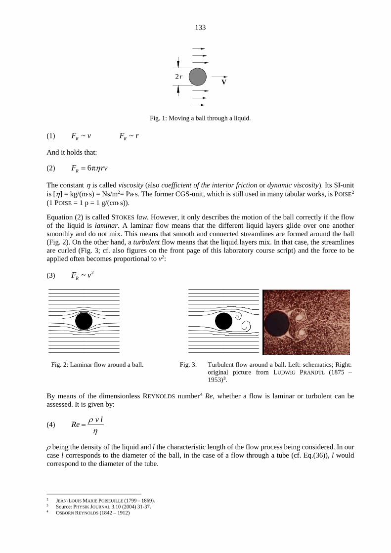
133

Fig. 1: Moving a ball through a liquid. (1) ~ ~R RF v F r And it holds that:

(2) 6πRF rvη= The constant η is called viscosity (also coefficient of the interior friction or dynamic viscosity). Its SI-unit is [η] = kg/(m⋅s) = Ns/m2= Pa⋅s. The former CGS-unit, which is still used in many tabular works, is POISE2 (1 POISE = 1 p = 1 g/(cm⋅s)). Equation (2) is called STOKES law. However, it only describes the motion of the ball correctly if the flow of the liquid is laminar. A laminar flow means that the different liquid layers glide over one another smoothly and do not mix. This means that smooth and connected streamlines are formed around the ball (Fig. 2). On the other hand, a turbulent flow means that the liquid layers mix. In that case, the streamlines are curled (Fig. 3; cf. also figures on the front page of this laboratory course script) and the force to be applied often becomes proportional to v2:

(3) 2~RF v

Fig. 2: Laminar flow around a ball. Fig. 3: Turbulent flow around a ball. Left: schematics; Right: original picture from LUDWIG PRANDTL (1875 – 1953)3.

By means of the dimensionless REYNOLDS number4 Re, whether a flow is laminar or turbulent can be assessed. It is given by:

(4) v lRe ρ

η=

ρ being the density of the liquid and l the characteristic length of the flow process being considered. In our case l corresponds to the diameter of the ball, in the case of a flow through a tube (cf. Eq.(36)), l would correspond to the diameter of the tube.

2 JEAN-LOUIS MARIE POISEUILLE (1799 – 1869). 3 Source: PHYSIK JOURNAL 3.10 (2004) 31-37. 4 OSBORN REYNOLDS (1842 – 1912)

V2 r

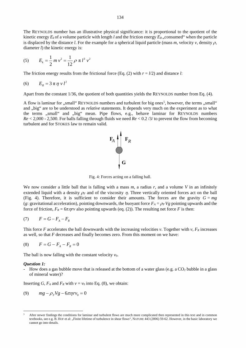
134

The REYNOLDS number has an illustrative physical significance: it is proportional to the quotient of the kinetic energy Ek of a volume particle with length l and the friction energy ER „consumed“ when the particle is displaced by the distance l. For the example for a spherical liquid particle (mass m, velocity v, density ρ, diameter l) the kinetic energy is:

(5) 2 3 21 1 π2 12kE m v l vρ= =

The friction energy results from the frictional force (Eq. (2) with r = l/2) and distance l:

(6) 23 πRE v lη= Apart from the constant 1/36, the quotient of both quantities yields the REYNOLDS number from Eq. (4). A flow is laminar for „small“ REYNOLDS numbers and turbulent for big ones5, however, the terms „small“ and „big“ are to be understood as relative statements. It depends very much on the experiment as to what the terms „small“ and „big“ mean. Pipe flows, e.g., behave laminar for REYNOLDS numbers Re < 2,000 - 2,500. For balls falling through fluids we need Re < 0.2 /3/ to prevent the flow from becoming turbulent and for STOKES law to remain valid.

Fig. 4: Forces acting on a falling ball. We now consider a little ball that is falling with a mass m, a radius r, and a volume V in an infinitely extended liquid with a density ρF and of the viscosity η. Three vertically oriented forces act on the ball (Fig. 4). Therefore, it is sufficient to consider their amounts. The forces are the gravity G = mg (g: gravitational acceleration), pointing downwards, the buoyant force FA = ρF Vg pointing upwards and the force of friction, FR = 6πηrv also pointing upwards (eq. (2)). The resulting net force F is then:

(7) A RF G F F= − − This force F accelerates the ball downwards with the increasing velocities v. Together with v, FR increases as well, so that F decreases and finally becomes zero. From this moment on we have:

(8) 0A RF G F F= − − = The ball is now falling with the constant velocity v0. Question 1: - How does a gas bubble move that is released at the bottom of a water glass (e.g. a CO2 bubble in a glass

of mineral water)? Inserting G, FA and FR with v = v0 into Eq. (8), we obtain:

(9) 06 0Fmg Vg rvρ πη− − =

5 After newer findings the conditions for laminar and turbulent flows are much more complicated then represented in this text and in common

textbooks, see e.g. B. HOF et al: „Finite lifetime of turbulence in shear flows“, NATURE 443 (2006) 59-62. However, in the basic laboratory we cannot go into details.

G

FFA R

135

Inserting m = ρKV (with ρK : density of the material) as well, and 343

V rπ= , we obtain from Eq. (9):

(10) ( )30

4 6 03 K Fr g rvπ ρ ρ πη− − =

Rearranging this equation for η, we obtain

(11) ( )2

0

29

K Fr gv

ρ ρη

−=

A simple method for an indirect measurement of η follows from Eq. (11), provided that ρK and ρF are known: One drops balls of radius r in the liquid to be analysed and measures their falling velocity v0 once the state F = 0 has been reached. There is a problem with this method: In general we do not deal with infinitely extended liquids, but, e.g. a cylinder of radius R, in which the falling of the balls is observed. In these cases, the additional friction of the liquid swept away by the ball along the cylinder’s wall must be taken into account. It leads to the fact that the measured velocity vm is lower than the velocity v0 in the case of an infinitely extended fluid. Since the deviation of vm from v0 depends mainly on the ratio of the cross sectional areas of the ball and the cylinder used, we can approximate vm by:

(12) 2

0mrv v kR

≈ −

where k is an experimentally determined correction factor6. With this, it follows:

(13) 2

0 mrv v kR

≈ +

2.2 Determining the Viscosity Using a Capillary Viscometer According to UBBELOHDE

A fluid flows through a vertical capillary of the radius r0. The period ∆t, which a liquid volume V takes to flow through the capillary is determined by the viscosity η of the liquid. The greater η, the greater ∆t. Capillary viscometers function according to this simple principle. Fig. 5 shows such a capillary viscometer following UBBELOHDE, which is described in more detail in Chap. 3.2 and in Appendix 4.4. The exact derivation of the quantitative relationship between η and ∆t is time-consuming. The derivation is presented in the Appendix 4.4. Here, only the result is given: (14) K tη ρ= ∆ Here, ρ is the density of the liquid and K a meter constant of the viscometer employed, into which the passed volume V enters among others (Fig. 5). For the kinematic viscosity υ= η/ρ with the unit [υ] = m2/s we obtain: (15) K tυ = ∆ In Eq. (14) and (15), a correction has to be made. Upon entering the narrow capillary from the large basin B (Fig. 5) of the capillary viscometer, the liquid must be accelerated according to BERNOULLI’s law7. The

6 Eq. (13) is an empirically discovered law for the experimental setup used. The correction by LADENBURG (c.f. /2/, for example), which is used

frequently, yields distinctly worse results for this experimental setup. 7 DANIEL BERNOULLI (1700 – 1782).

136

required work leads to a small drop in pressure, which causes an increase in the efflux time ∆t. Therefore, time correction terms tk are to be subtracted from the measured times ∆t (HAGENBACH’s correction), which are supplied by the manufacturers of the UBBELOHDE viscometers as meter constants. Hence, the final equation for determining the kinematic viscosity reads:

(16) ( )kK t tυ = ∆ −

Fig. 5: Capillary viscometer according to Ubbelohde. During the time ∆t the volume V flows through the capillary

(red) of radius r0 and length l. For further labels, refer to Chap. 3.2 and Appendix 4.4.

2.3 Laminar and Turbulent Pipe Flows

Fig. 6 shows a setup that can be used to measure the transition of a laminar flow to a turbulent one in a cylindrical pipe8. A liquid, water in this case, flows through a long plexiglass pipe of bore diameter d. The water flows into the pipe from a reservoir. The reservoir is replenished though an inlet (a faucet). An overflow is used to maintain a constant water level in the reservoir, so that the pressure at the pipe’s inlet remains constant. A sieve serves to calm the incoming water-flow. The velocity v of the flow can be adjusted by the faucet H1 at the end of the pipe. In addition to the water from the reservoir, a thin jet of coloured water is injected through a nozzle into the centre of the pipe. The strength of the current through the nozzle can be adjusted by a faucet H2.The jet of coloured water is seen as a smooth stream filament for small flow velocities v. If the flow velocity is increased slowly by opening the faucet H1, the current filament will begin to exhibit eddies starting at a certain velocity vt, thus showing the transition from a laminar to a turbulent flow. By measuring the volume of flow per time in this setting of the faucet H1, the flow velocity vt can be determined and the corresponding REYNOLDS number Re may be calculated:

(17) w t

w

v dRe ρη

=

8 By recommendation of A. HEIDER, DEUTSCHES ZENTRUM FÜR LUFT- UND RAUMFAHRT (DLR), Göttingen.

G

D H

M

M

V1

2

l

2 3 1

B

2r0

137

where ρw and ηw are the density and viscosity of the water.

Fig. 6: Setup for measuring the transition of a laminar to a turbulent flow in a pipe having inner diameter d. For

details, refer to the text. Details for the quantitative description of the water flow through a pipe are given in Appendix 4.3.

3 Experimental Procedure Equipment:

Six glass cylinders with different diameters in adjustable stand with water level, seals for the cylinders with a drill hole in their centres, 2 l vessel containing glycerine-water mixture, steel balls (about 100 balls with d ≈ 2 mm), forceps, analytical balance (precision 0.001 g), laboratory balance (precision 0.01 g), micrometer gauge, slide measuring gauge, stop watch, thermometer (precision 0.1 C), magnet, UBBELOHDE viscometer (K ≈ 10-8 m2/s2) in mounting and water bath, suction tube, ethanol, mounted flow tube (d = (12.10 ± 0.05) mm) with water reservoir, water with food color, measuring cylinder (100 ml and 1000 ml), bucket, floor cloth, kitchen paper roll.

3.1 Determining the Viscosity of a Glycerine-Water Mixture by Means of the Falling-Ball Method

Remarks: - The mixing ratios of the glycerine-water mixtures are not identical in all experiments. Since the viscosity

strongly depends on the mixing ratio and the temperature (cf. Chap. 4.1 and 4.2), every working group must perform the whole experiment at constant room temperature using the mixture from one storage basin!

- The work place has to be tidied before leaving! Using a set-up as shown in Fig. 7 the falling movement of steel balls (d = 2r ≈ 2 mm) in a glycerine-water mixture is to be investigated with the aim of determining the viscosity of the mixture according to Eq.(11). In order to quantify the influence of frictional effects at the wall of the basin (cf. Eq. (13)), various glass cylinders with different radii R are used. The experiment is prepared by determining the following quantities:

(a) Density ρF of the mixture using a laboratory balance by weighing a volume determined with a measuring cylinder.

(b) Mean radius r of the balls by measuring the diameters of at least ten balls using the micrometer gauge and subsequently calculating the mean value.

(c) Density ρK of the ball material by weighing n balls (n ≥ 100) by means of an analytical balance.

d

Zulauf

Überlauf

H

H

Düse

Farbe

Ablauf Ablauf

1

2

Flies

138

(d) Radii R of the glass cylinders used by measuring the inner diameter using a slide measuring gauge. (e) Temperature of the mixture. Since the viscosity strongly depends on the temperature, it is only

reasonable to record a result if the temperature of the mixture is simultaneously recorded. Keep room temperature as constant as possible during the experiment!

Fig. 7: Set-up of falling-ball experiment in liquids. The spheres of radius r fall through the upper drilled seal (grey).

This is to ensure that they fall into the liquid (beige), contained in a cylinder with bore radius R, as close to the centre of the cylinder as possible.

Following the above preparations, the glycerine-water mixture is carefully filled into six glass cylinders with different radii R (avoid bubble formation!). The fluid level must be below the bottom of the seal. Subsequently the cylinders are fixed in the mount (by careful tightening of the plastic screws) and the base plate of the mount is vertically adjusted using an integrated water level. The cylinders are now positioned vertically. Then ten balls are dropped centrally into each cylinder. For centring, a suitable seal with a drill-hole in its centre is used (Fig. 7). The time t it takes to fall a distance s, which is determined by the two horizontal mounting brackets on the cylinders (s measured with the caliper), is measured using a stop watch. The start of the distance s (upper mounting bracket) must be a few centimetres below the surface of the liquid. Question 2: - Why should the distance of the fall not begin at the surface of the liquid? Question 3: - Why is it important to drop the balls into the centre of the cylinder? For every glass cylinder the sinking velocity

(18) msvt

=

is determined, t being the mean value of the measured time for falling for each of the ten balls. Subse-quently, vm is plotted against (r/R)2 (with error bars for vm) and a regression line through the measured data is determined. The intersection of the line with the vm-axis determines the velocity v0 for an infinitely extended liquid (R → ∞). From the data obtained by this experiment for v0, r, ρK, and ρF as well as from the gravitational acceleration for Oldenburg (g = 9.8133 m/s2, error negligible9), the viscosity η of the glycerin-water mixture is determined according to Eq. (11) and the result is compared with the data from Table 1 (Chap. 4.1). After completion of the measurement the liquid is carefully (again preventing the formation of bubbles!) poured from the glass cylinders back into the storage vessel using a sieve in order to collect the balls. The

9 Value taken from http://www.ptb.de/cartoweb3/SISproject.php; the error of 2×10-5 m/s2 is neglected.

2 r

vm

s

2 R

139

balls remaining in the glass cylinders are removed with a magnet. The balls are cleaned in water and dried with crepe paper.

3.2 Determining the Kinematic Viscosity Using a Capillary Viscometer The kinematic viscosity of ethanol at room temperature is to be determined using a capillary viscometer according to UBBELOHDE. The viscometer is placed into a large water bath which provides a constant temperature (to be measured!) within the capillary throughout the experiment. Prior to the experiment the technical assistant adjusted the viscometer vertically and filled the storage basin H above tube 1 (cf. Fig. 5) with ethanol up to about three quarters. Tube 3 is closed with a finger. By means of a suction tube connected with tube 2 the liquid is sucked up into tube 2 until the overhead flask G is completely filled. Then tubes 2 and 3 are opened and the time ∆t during which the liquid level drops from mark M1 to mark M2 is determined. The measurement is repeated three times. The kinematic viscosity υ of ethanol for the predominant temperature of the water bath is determined from the measured values and the available meter constants K and tk, and is then compared with values stated in the literature.

3.3 Determination of the REYNOLDS Number at the Transition from Laminar to Turbulent Pipe Flow

With a setup according to Fig. 6 the REYNOLDS number at the transition from a laminar to a turbulent pipe flow is to be determined. At first, the faucet controlling the flow to the reservoir is opened far enough, ensuring that the water level in the reservoir is just maintained at the level of the overflow during the whole experiment. The tube from the drain of the pipe is placed in the outlet. The faucet H1 at the end of the pipe is opened slowly until water flows from the end of the pipe. At small flow velocities, the flow in the pipe is laminar. Next, the faucet H2 is opened far enough, so that a thin, straight stream filament becomes visible. Now, the faucet H1 is slowly opened further until the laminar flow changes to a turbulent one. This can be observed by the stream filament beginning to “jitter”. To measure the flow velocity v for the current position of the faucet H1, a measuring cylinder is placed underneath the output tube of the pipe for a time interval ∆t (measured with a stop watch) in order to capture the water. From the volume V, the (inner) diameter d of the pipe, the density10 and the viscosity η of the water (c.f. Appendix 4.2), the flow velocity v, and thus, the REYNOLDS number Re may be determined.

4 Appendix 4.1 Viscosity of Glycerine Glycerine11 (C3H8O3) is hygroscopic, i.e. it adsorbs water. If it is exposed to the air for some time, it absorbs humidity from the ambient air. Thus a mixture with an increasing water content is formed over the course of time. The viscosity of such a mixture differs from that of pure glycerine. For your guidance some data for a temperature of 20 °C are stated in Table 1:

Table 1: Viscosity of glycerine/water mixtures at 20 °C.12

C3H8O3 weight-%

H2O weight-%

η / kg m-1s-1

100 0 1,76 96 4 0,761 92 8 0,354 88 12 0,130 84 16 0,071 80 20 0,048

10 For the temperature-dependent density of water, see the experiment “Surface tension…”. 11 Further common names for glycerine are glycerol, propan-1,2,3-triol and others. The structure is described by C3H5(OH)3 . 12 Data after: WEAST, R. C. [Ed.]: „CRC Handbook of Chemistry and Physics”, 56th Ed., CRC Press, Boca Raton, 1975 - 1976. All data without

error statement.

140

In addition, the viscosity is strongly dependent on temperature. For pure glycerine at T = 20 °C: η = 1,76 kg/(m s) (see above) and at T = 25 °C: η = 0,934 kg/(m s)13

4.2 Viscosity of Water Fig. 8 shows the viscosity η of water as a function of temperature T. In the temperature interval between 10 °C and 35 °C, the data can be described in good approximation by a polynomial of degree 4 (T in °C)12:

(19)

2

33 45 8

1,77721 - 0,05798 + 0,00125 kg10m s-1,66039 10 9,814 10

T T

T Tη −

− −

≈ ⋅ + ⋅

Fig. 8: Viscosity η of water as a function of temperature T.

4.3 Laminar Pipe Flow This appendix details how the flow velocity v and its lateral profile v(r) in a cylindrical pipe may be cal-culated quantitatively.14 An ideal liquid is incompressible and free of internal friction forces. We consider (as shown in Fig. 9) such a liquid flowing through a tapering horizontal tube. The incompressibility of the liquid means that the rate of volume flow Q (flowing volume per time) must be identical everywhere in the tube. A1 is the cross-sectional area of the tube and v1 the flow velocity on the left side of the tube, A2 and v2 are the corresponding quantities on the right side. This means:

(20) 1 1 2 2 const.VQ A v A vt

∆= = = =

∆

Eq. (20) is called the continuity equation. To move a fluid volume ∆V from the left side of the tube to the right side by ∆x1, the work W1 has to be performed by the static pressure p1 on the left side:

(21) 1 1 1 1 1 1 1W F x p A x p V= ∆ = ∆ = ∆

13 LIDE, D. R. [Ed.]: "CRC Handbook of Chemistry and Physics on CD-ROM", Taylor & Francis, Boca Raton, FL, 2006. All data without error

statement. 14 r is the lateral distance from the axis along the pipe.

10 20 30 400,6

0,7

0,8

0,9

1,0

1,1

1,2

1,3

1,4

η / 1

0-3 k

g m

-1 s-1

T / °C

141

The required work W2 for moving the same volume ∆V through the right side of the tube against the static pressure p2 is given by:

(22) 2 2 2 2 2 2 2W F x p A x p V= ∆ = ∆ = ∆

Fig. 9: Flow through a tapering horizontal tube. See text for labels. From the law of conservation of energy it follows that the energy difference W1 - W2 must lead to an increase in the kinetic energy of the liquid (density ρ) on the right side of the tube. If m is the mass and v1, v2 are the velocities of the volumes ∆V, it follows:

(23) 2 2 2 21 2 1 2 2 1 2 1

1 1 1 12 2 2 2

W W p V p V m v m v V v V vρ ρ− = ∆ − ∆ = − = ∆ − ∆

Following division by ∆V and resorting the terms we finally obtain:

(24) 2 2 21 1 2 2

1 1 1: const.2 2 2

p v p v p vρ ρ ρ+ = + = + =

which is BERNOULLI's law. It says that according to the stated assumptions, the sum of the static pressure p and dynamic pressure ½ρv2 must be constant everywhere in the tube. The hydrostatic pressure ρgh which depends on the height h has to be considered if we have a vertical tube instead of a horizontal one (g is the gravitational acceleration). Then BERNOULLI’s law reads:

(25) 21 const.2

p v ghρ ρ+ + =

Pressure and flow velocity are constant in the entire horizontal tube if the tube's diameter is constant and if an ideal liquid flows through it. In the case of a real fluid with the viscosity η friction forces appear between the fluid and the material of the tube and between the neighbouring fluid layers. These friction forces cause the pressure along the tube to decrease and the flow velocity to vary along the tube's cross-section, thus in the lateral direction. It must be zero on the boundary (because a boundary layer of the liquid adheres to the wall) and must assume its maximum value in the centre. For a quantitative description of the transverse velocity profile of a laminar tube flow we consider (as in Fig. 10) a cylindrical tube with the length l and the radius r0 in which a real fluid flows along the z-axis. Within this flow we observe a co-axial liquid cylinder with radius r and lateral surface area A = 2πrl. According to NEWTON's law of friction the friction force FR between this liquid cylinder and the adjacent layer of liquid is proportional to the lateral surface area A and to the velocity gradient dv/dr. The propor-tionality constant is the viscosity η:

∆V

p

F

∆ x2

2

2F1

A2

A

p1

∆ x1

1

142

(26) 2Rdv dvF A r ldr dr

η π η= =

Fig. 10: Cylindrical tube with co-axial liquid cylinder of radius r. Pressure p1 is on the left side; pressure p2 is on

the right side. For other labels, please refer to the text. In the stationary case (temporally constant flow velocity) the friction force FR for a fluid cylinder with the radius r must just equal the driving force F caused by the pressure gradient ∆p = p1 - p2, thus:

(27) 2 2 d vF r p r ld r

π π η= ∆ =

From this we obtain:

(28) 2

d v p rd r lη

∆=

and

(29) d d2

pv r rlη

∆= , respectively,

and finally by the integration with the boundary condition v(r0) = 0 the desired velocity profile v(r):

(30) ( )2 20 0( ) ; 0

4pv r r r r rlη

∆= − ≤ ≤

Thus, the transverse velocity profile of a laminar flow through a tube is parabolic (cf. Fig. 11). For calculating the volume V, which flows through the cylinder with a radius r0 during the time ∆t, we first look at the volume flow ∆V/∆t through a hollow cylinder with an inner radius r and an outer radius r + dr (cf. Fig. 12). This hollow cylinder has the cross sectional area A and length ∆l. For a small wall thickness dr, the volume flow is given by:

(31) d 2π dV A l lr r

t t t∆ ∆

= =∆ ∆ ∆

Since the liquid flows through the tube uniformly (i.e. without acceleration), it follows that the velocity is:

(32) lvt

∆=

∆

p2

r0

r z

1p

F

l

143

Fig. 11: Left: Calculated parabolic velocity profile of a laminar flow through a cylindrical pipe with the radius r0.

Right: Visualization of a parabolic velocity profile in a cylindrical plexiglass pipe (diameter about 1 cm) with the aid of coloured glue.15

Applying Eq. (30), Eq. (31) thus becomes:

(33) ( )2 20

d 2π d ( ) 2π d4

V pr r v r r r r rt lη

∆= = −

∆

Fig. 12: Definition of the geometrical dimension of a hollow cylinder.

From this equation, by integration, we may calculate the net volume V flowing through the tube with the radius r0 within the time ∆t:

(34) ( )Vt

pl

r r r drr

∆∆

= −∫π

η2 02 2

0

0

and thus

(35) 408

p tV rl

πη

∆ ∆=

This is the HAGEN-POISEUILLE16 law for laminar flows. They appear when REYNOLDS number Re, here:

(36) 02v rRe= ρη

(ρ: density of the liquid; v : mean value of the flow velocity according

to Eq. (30) is smaller than about 2,000 - 2,500.

15 Source: T. GREVE: „Aufbau und physikalische Betrachtung eines Durchlaufreaktors zur Hydrothermalen Karbonisierung“, Diploma thesis,

Carl von Ossietzky Universität Oldenburg, Institut für Physik, AG Turbulenz, Windenergie und Stochastik (TWiST), 2009. 16 GOTTHILF HEINRICH LUDWIG HAGEN (1797 – 1884)

-1,0 -0,8 -0,6 -0,4 -0,2 0,0 0,2 0,4 0,6 0,8 1,0

1,0

0,8

0,6

0,4

0,2

0,0

v(r)

/ b.E

.

r / r0

∆ l

d r

r

A

144

4.4 Capillary Viscometer In this appendix, the derivation of Eq. (14) is explained. By means of the HAGEN-POISEUILLE law (Eq. (35)) we are able to determine the viscosity of fluids. For this we use a capillary viscometer. Fig. 5 shows a capillary viscometer according to UBBELOHDE. A defined volume of liquid V flows from a storage basin B with an overhead flask G through a capillary with the radius r0 and the length l. The volume of liquid is defined by the volume between the marks M1 und M2. The viscosity η can be determined using Eq. (35) by measuring the time difference ∆t in which the liquid mirror surface drops from M1 to M2 :

(37) 4

0

8p r t

lVπη ∆

= ∆

In this case, the pressure difference ∆p is given by the hydrostatic pressure: (38) ( ) ( )p t g h tρ∆ = (ρ: density of liquid; g: gravitational acceleration) h(t) being the altitude difference between the momentary level of the liquid mirror surface in the basin and the lower end of the capillary. We use a trick so that the lower end of the capillary represents the reference level: by means of the ventilation tube 3 (cf. Fig. 5) there is air pressure in the overhead flask D. Conse-quently the liquid flows off in the form of a thin film along the inner wall of D. Due to the time-dependence of the height h(t) (dropping liquid mirror surface), ∆p(t) is also time-dependent. However, h(t) may be replaced by a suitable mean value. This mean height h is given by:

(39) 0

1 ( )t

h h t dtt

∆

=∆ ∫

Hence it follows from Eq. (37):

(40) 4

0

8g h r tlV

π ρη = ∆

The quantity

(41) 4

0

8g h rKlV

π=

is a meter constant and is engraved into the viscosimeter ([K] = m2/s2; mostly given in mm2/s2). This yields the simple relationship for the viscosity following Eq.(14): K tη ρ= ∆

145

Carl von Ossietzky University Oldenburg – Faculty V - Institute of Physics Module Introductory laboratory course physics – Part I

Translation of German denotations in figures of the script for the module

Introductory Laboratory Course Physics – Part I German English Ablauf (aus einem Gefäß) drain (from a vessel) Abtastpunkte sampling points Abtastungs-Erfassungsintervalle sampling intervals Additionsverstärker add amplifier Amboss anvil Amperemeter ammeter Anschlussbuchse contact Anschlusskontakt contact Aufhängung suspension Ausgleichsgerade regression line außen external Außenleiter outer conductor Außenmessschenkel outside jaw Biegestab bending rod Bits auf 0 bits to 0 Blech mit Schlitz sheet with slit Blech mit Spalt sheet with slit BNC-Buchse BNC socket BNC-Stecker BNC plug Chemie chemistry DMS (Dehnungsmessstreifen) SG (strain gauge) Druck pressure dunkel dark Düse jet Einheiten units Einheit zur Einstellung von z.B. unit for adjusting e.g. Elektroden electrodes elektronisch gesteuerter Schalter electronically controlled switch Erde earth potential, ground Erfassung recording erzeugt Ausgangsimpuls wenn Eingangsspannung > Schwellwert

produces output impulse if initial voltage > threshold

Fächer subjects Farbe colour Feder spring Fehler der Summe der Quadrate error of the sum of the squares Fläche surface Flies sieve Flüssigkeit liquid Flüssigkeitslamelle liquid lamella Funktionsgenerator function generator Gas gas Geflecht mash Gehäuse case getriggert triggered Gewichtung, keine Gewichtung weighting

146

Gleichung equation Glimmstarter glow starter globales Minimum global minimum GND-Linie ground line hell light horizontal horizontal Hilfe help Impuls (getriggert) pulse (triggered) innen interior Innenleiter inner conductor Innenmessschenkel inside jaw Intensität intensity Isolierung insulation Koaxialkabel coaxial cable Kommentare comments Kondensator capacitor Kraftmesser dynamometer Laborkabel laboratory cable Langname long name Leiter conductor Leitungskreuzung line intersection Leuchtstoff luminescent material Licht light Lineare Anpassung linear fit lokales Minimum local minimum Luft air Luftzufuhr air supply Mantel cladding Masse ground Massekontakt ground contact Mathematik mathematics Matrikelnr. registration number Menü menu Messdaten measured data Messhülse measuring sleeve Messschiene measure scale Messspindel measure spindle Messtrommel no translation Messung measurement Metallring metal ring Mittelwert mean value Monitor monitor Nachname last name Netzgerät power supply Netzspannung line voltage Nonius vernier Normale Abtastung normal sampling Oszilloskop oscilloscope Parameter parameter Pegel auf 50% level set to 50 % Physik physics Piezoresistives Si-Element piezoresistive Si-element Probekörper test specimen Ratsche ratched stop

147

Schaltung wiring Schnittpunkt mit der Y-Achse intersection with the Y-scale schwarz (Masse) black (ground) Schwellwertdiskriminator threshold discriminator Semester term Signalleitung signal line Si-Membran Si-membrane Spannungsquelle voltage source speichern store Spitzenwert peak value Spule coil Standardfehler standard error Steigung slope Stromquelle current source Student student Tiefenmessschiene depth measure scale Triggerflanke trigger slope Triggerschwelle trigger level Triggerzeitpunkt trigger time Trigger Zwang force trigger Überlauf overflow Umschalter ( 2-fach ) selector switch (2-fold) Verbindung connection Verstärker amplifier Verstärkungsfaktor amplification factor vertikal vertical Voltmeter voltmeter Vorname first name Wasser water Wellenfronten wave front Wert value Wertigkeit significance Widerstand resistance Zeitablenkung time base Zielgröße target value Zulauf (in ein Gefäß) inlet (into a vessel) Zustand state

Recommended values of some fundamental physical constants (2014) 1 Constant Symbol Value Unit Remark Atomic mass unit u 1,660 539 040 (20)⋅10-27 kg Avogadro constant NA 6,022 140 857 (74)⋅1023 mol-1 Boltzmann constant k 1,380 648 52 (79)⋅10-23 J/K Electric constant: 1/(µ0c2) ε0 8,854 187 817...⋅10-12 As/(Vm) exact Elementary charge e 1,602 176 6208 (98)⋅10-19 As Faraday constant F 96 485,332 89 (59) C/mol Constant of gravitation G 6,674 08 (31)⋅10-11 m3/(s2kg) Speed of light in vacuum c 2,99792458⋅108 m/s exact Magnetic constant: 4π⋅10-7 µ0 1,256 637 0614…⋅10-6 Vs/(Am) exact Molar gas constant R 8,314 4598 (48) J/(mol K) Planck constant h 6,626 070 040(81)⋅10-34 Js Electron mass me 9,109 383 56(11)⋅10-31 kg Neutron mass mn 1,674 927 351 (74)⋅10-27 kg Proton mass mp 1,674 927 471 (21)⋅10-27 kg Standard acceleration of gravity g 9,80665 m/s2 exact (Definition) The numbers in parentheses indicate the single standard deviation in units of the last decimal position. Prefixes

Factor Name Symbol Factor Name Symbol 10-1 deci d 101 deca da 10-2 centi c 102 hecto h 10-3 milli m 103 kilo k 10-6 micro µ 106 mega M 10-9 nano n 109 giga G

10-12 pico p 1012 tera T 10-15 femto f 1015 peta P 10-18 atto a 1018 exa E 10-21 zepto z 1021 zetta Z 10-24 yocto y 1024 yotta Y

1 Source: Peter J. Mohr; David B. Nevell; Barry N. Taylor: "CODATA Recommended Values of the Fundamental

Physical Constants: 2014", arXiv: 1507.07956v1 [physics.atom-ph] 21. of July 2015. See also: http://arxiv.org/pdf/1507.07956v1.pdf and http://physics.nist.gov/cuu/Constants/index.html.