Introductory Guide toUnix-SAS

Department of Mathematics and Statistics

Written by Julian Visch

SAS

Stress and suffering - Stress and suffering - Stress and s uff

erin

g-

Str

ess

and

suff

erin

g-S

tressand

suff

erin

g-

Stress

and

suffering-

Str

essand

suffering-St

ress

an

dsufferin

g-

Str

es s and suffe

When SAS first appeared on the scene it was an acronym for the StatisticalAnalysis System. Since that time SAS has become an integrated system ofsoftware products and wants to lose the astigmatism of being consideredjust a statistical analysis system. The name SAS is no longer consideredan acronym, but a name, and as such does NOT stand for anything.

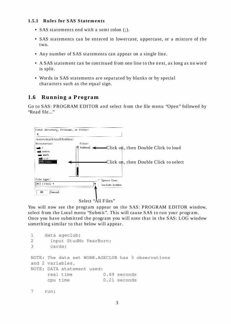
Contents

1 The Basics 11.1 Introduction . . . . . . . . . . . . . . . . . . . . . . . . . . . . . . . . . . 11.2 How to Create Your Own Programs . . . . . . . . . . . . . . . . . . . . . 1

1.2.1 Rules for SAS Names . . . . . . . . . . . . . . . . . . . . . . . . . 11.3 Starting SAS . . . . . . . . . . . . . . . . . . . . . . . . . . . . . . . . . . 11.4 Exiting SAS . . . . . . . . . . . . . . . . . . . . . . . . . . . . . . . . . . 21.5 Creating a Simple Program . . . . . . . . . . . . . . . . . . . . . . . . . 2

1.5.1 Rules for SAS Statements . . . . . . . . . . . . . . . . . . . . . . 31.6 Running a Program . . . . . . . . . . . . . . . . . . . . . . . . . . . . . . 3

1.6.1 Short Cuts . . . . . . . . . . . . . . . . . . . . . . . . . . . . . . . 41.7 Producing Output . . . . . . . . . . . . . . . . . . . . . . . . . . . . . . . 4

1.7.1 Output (Print) Options . . . . . . . . . . . . . . . . . . . . . . . . 51.7.2 Increasing the Default Page Size . . . . . . . . . . . . . . . . . . 5

1.8 Loading Data from a File . . . . . . . . . . . . . . . . . . . . . . . . . . . 51.9 Printing your Output . . . . . . . . . . . . . . . . . . . . . . . . . . . . . 51.10 Transferring Output to a File . . . . . . . . . . . . . . . . . . . . . . . . 61.11 Storing Permanent SAS Data Files . . . . . . . . . . . . . . . . . . . . . 61.12 Creating Subsets of Permanent Data Files . . . . . . . . . . . . . . . . 7

2 Ways for Inputting Data 82.1 Inserting Character Variables . . . . . . . . . . . . . . . . . . . . . . . . 82.2 List Input . . . . . . . . . . . . . . . . . . . . . . . . . . . . . . . . . . . . 8

2.2.1 Rules for List Input Statements . . . . . . . . . . . . . . . . . . . 82.3 Column Input . . . . . . . . . . . . . . . . . . . . . . . . . . . . . . . . . 9

2.3.1 Reading Embedded Blanks and Longer Variables . . . . . . . . 92.3.2 Picking and Choosing Variables . . . . . . . . . . . . . . . . . . . 9

2.4 Combining List and Column Inputs . . . . . . . . . . . . . . . . . . . . 102.5 Data Files with Different Formats . . . . . . . . . . . . . . . . . . . . . 102.6 Impossible Data Files . . . . . . . . . . . . . . . . . . . . . . . . . . . . . 102.7 Creating Dependent Variables . . . . . . . . . . . . . . . . . . . . . . . . 11

2.7.1 Logic Statements . . . . . . . . . . . . . . . . . . . . . . . . . . . 112.8 Use of “If” Statements . . . . . . . . . . . . . . . . . . . . . . . . . . . . 122.9 Deleting Observations . . . . . . . . . . . . . . . . . . . . . . . . . . . . 13

3 Odds and Ends 133.1 Defining Keys . . . . . . . . . . . . . . . . . . . . . . . . . . . . . . . . . 133.2 Including Comments within your SAS Program . . . . . . . . . . . . . 143.3 Sorting your Data . . . . . . . . . . . . . . . . . . . . . . . . . . . . . . . 14

3.3.1 Sorting by more than one Variable . . . . . . . . . . . . . . . . . 143.3.2 Sorting in Descending Order . . . . . . . . . . . . . . . . . . . . 153.3.3 Removing Duplicates . . . . . . . . . . . . . . . . . . . . . . . . . 15

3.4 Using the Inbuilt Help Facility . . . . . . . . . . . . . . . . . . . . . . . 153.5 Using the Means Procedure . . . . . . . . . . . . . . . . . . . . . . . . . 163.6 Calculating Correlations and Covariances . . . . . . . . . . . . . . . . . 16

i

4 SAS Graphics 164.1 Low Level Graphics (Scatter Plots) . . . . . . . . . . . . . . . . . . . . . 16

4.1.1 Adding Title and Labels to a Plot . . . . . . . . . . . . . . . . . . 174.1.2 Modifying Tickmarks . . . . . . . . . . . . . . . . . . . . . . . . . 174.1.3 Specifying Plotting Symbols . . . . . . . . . . . . . . . . . . . . . 174.1.4 Creating Multiple Plots . . . . . . . . . . . . . . . . . . . . . . . 174.1.5 Creating Multiple Plots on the Same Page . . . . . . . . . . . . 174.1.6 Creating Multiple Plots on the Same Axes . . . . . . . . . . . . . 18

4.2 Low Level Graphics (Bar Plots) . . . . . . . . . . . . . . . . . . . . . . . 184.2.1 Specifying Midpoint Values . . . . . . . . . . . . . . . . . . . . . 194.2.2 Specifying Number of Midpoints . . . . . . . . . . . . . . . . . . 194.2.3 Charting every Value . . . . . . . . . . . . . . . . . . . . . . . . . 194.2.4 Creating Subgroups within a Range . . . . . . . . . . . . . . . . 204.2.5 Grouping Bars . . . . . . . . . . . . . . . . . . . . . . . . . . . . . 20

5 High Level Graphics 205.1 Scatter Plots . . . . . . . . . . . . . . . . . . . . . . . . . . . . . . . . . . 20

5.1.1 Adding a Title . . . . . . . . . . . . . . . . . . . . . . . . . . . . . 205.2 Bar Plots . . . . . . . . . . . . . . . . . . . . . . . . . . . . . . . . . . . . 21

5.2.1 Bar Plots with Subgroups . . . . . . . . . . . . . . . . . . . . . . 215.3 Pie Charts . . . . . . . . . . . . . . . . . . . . . . . . . . . . . . . . . . . 225.4 Graphic Options . . . . . . . . . . . . . . . . . . . . . . . . . . . . . . . . 225.5 Printing Graphs . . . . . . . . . . . . . . . . . . . . . . . . . . . . . . . . 235.6 Graphics to file → graphics to screen . . . . . . . . . . . . . . . . . . . . 23

6 Exercises 24

7 Appendix 25

ii

1 The Basics

1.1 Introduction

When programming in any package the 8 crucial things you must learn when youstart are

• How to start the package.

• How to exit the package.

• How to create and edit programs for running within the package.

• How to run the aforementioned programs.

• How to load data into the package.

• How to produce output within the package.

• How to produce printed versions of the aforementioned output.

• How to transfer output to a file.

1.2 How to Create Your Own Programs

As the program editor in SAS is not easy to work with you are advised to open up anew file using your favourite editor (e.g xedit hobbes1). For reference I have titledthe initial SAS file hobbes1, your title may differ.

1.2.1 Rules for SAS Names

• A SAS name can contain from one to eight characters.

• The first character must be a letter or an underscore “ ”.

• Subsequent characters must be letters, numbers, or underscores.

• Blanks cannot appear in SAS names.

1.3 Starting SAS

To get onto SAS type “SAS &” (without the quotes) in the directory in which youintend to write your macros/programs.e.g If my file hobbes1 was stored in the directory /users/math/staff/hobbes/sas thenI would run SAS from the same directory.

1

Three windows will now appear with a fourth being automatically iconised. Thewindows are

• SAS: OUTPUTThis window displays all the output generated from your programs, hence thename.

• SAS: LOGThis window displays any error messages that occur because of bugs in yourprograms.

• SAS: PROGRAM EDITORThis window is where you retrieve, write, modify or submit(run) your pro-grams.

• SAS: SessionThe xsassm client provides a convenient way of iconising or mapping the win-dows associated with its SAS client session, or interrupting and terminatingits associated SAS client session via the UNIX signal mechanism.

Note: it is important to place the SAS: PROGRAM EDITOR near the top of thescreen because later when you try and open a file a dialog box will appear which ispositioned according to where the SAS: PROGRAM EDITOR is.

1.4 Exiting SAS

Either click “Terminate” on the SAS: SESSION window or select exit from the filemenu.

1.5 Creating a Simple Program

All SAS programs are made up of one or more procedures, your first program willconsist of just one simple procedure.Firstly we will enter the following into our file “hobbes1”

data ageclub; ←�

tells SAS to create a temporarydata set called ageclub.

input StudNo YearBorn; ← specifies variable names.cards; ← specifies that the data will follow.

123 88101 89 ← the data.432 90run; ← specifies the end of the procedure.

Note: It is important to note that tabs are not the same as spaces, therefore makesure no tabs exist in your data, as otherwise you may encounter problems when yourun your sas programs.

2

1.5.1 Rules for SAS Statements

• SAS statements end with a semi colon (;).

• SAS statements can be entered in lowercase, uppercase, or a mixture of thetwo.

• Any number of SAS statements can appear on a single line.

• A SAS statement can be continued from one line to the next, as long as no wordis split.

• Words in SAS statements are separated by blanks or by specialcharacters such as the equal sign.

1.6 Running a Program

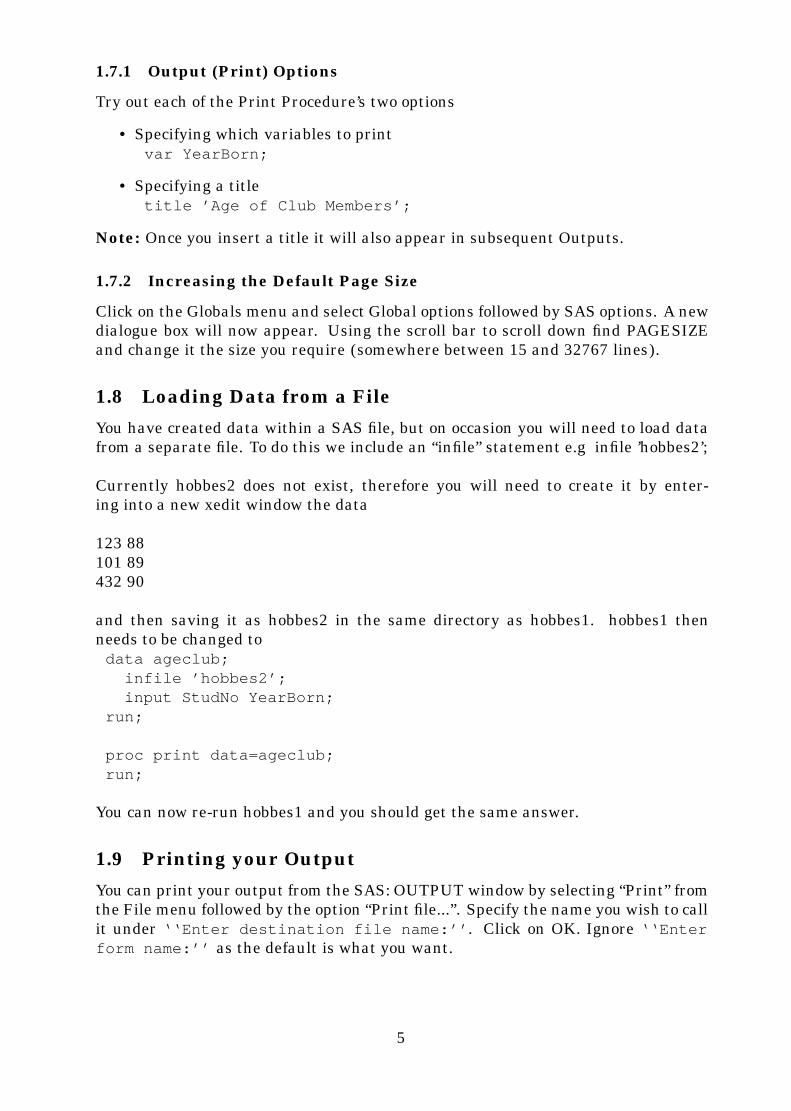
Go to SAS: PROGRAM EDITOR and select from the file menu “Open” followed by“Read file...”

/users/math/staff/hobbes/

staffhobbes Click on, then Double Click to select

Click on, then Double Click to load

Select “All Files”You will now see the program appear on the SAS: PROGRAM EDITOR window,select from the Local menu “Submit”. This will cause SAS to run your program.Once you have submitted the program you will note that in the SAS: LOG windowsomething similar to that below will appear.

1 data ageclub;2 input StudNo YearBorn;3 cards;

NOTE: The data set WORK.AGECLUB has 3 observationsand 2 variables.NOTE: DATA statement used:

real time 0.69 secondscpu time 0.21 seconds

7 run;

3

The SAS: LOG window shows how SAS went step by step through your programadding appropriate comments as it goes through the steps. Should you have madean error in writing your program then some comment to that effect will also appearhere.

1.6.1 Short Cuts

For the cases where you have only a portion of a program to run you can skip the“loading in stage” by firstly selecting with the mouse your entire program and thenselecting from the “local” menu “submit clipboard”. Try selecting hobbes1 and then“submit clipboard”.

To rerun entire programs quickly write in the program editor

%inc ’hobbes1’;run;

and then select “submit”. Then to repeat it just select “recall text” followed by“submit”.

1.7 Producing Output

To see some output you need to add the print procedure to your program.

proc print data=ageclub; ←

8>>>>>>>><>>>>>>>>:

Specifies which data set toprint. If you omit thedata=ageclub, the print pro-cedure processes the mostrecently created SAS dataset in the program.

Any additional options would be inserted hererun;

Now re-run your program (see Subsection 1.6.1).You should now get the following in your output window.

The SAS System 109:38 Monday, June 10, 1996

OBS STUDNO YEARBORN

1 123 882 101 893 432 90

Date of submissionPage number

4

1.7.1 Output (Print) Options

Try out each of the Print Procedure’s two options

• Specifying which variables to printvar YearBorn;

• Specifying a titletitle ’Age of Club Members’;

Note: Once you insert a title it will also appear in subsequent Outputs.

1.7.2 Increasing the Default Page Size

Click on the Globals menu and select Global options followed by SAS options. A newdialogue box will now appear. Using the scroll bar to scroll down find PAGESIZEand change it the size you require (somewhere between 15 and 32767 lines).

1.8 Loading Data from a File

You have created data within a SAS file, but on occasion you will need to load datafrom a separate file. To do this we include an “infile” statement e.g infile ’hobbes2’;

Currently hobbes2 does not exist, therefore you will need to create it by enter-ing into a new xedit window the data

123 88101 89432 90

and then saving it as hobbes2 in the same directory as hobbes1. hobbes1 thenneeds to be changed todata ageclub;infile ’hobbes2’;input StudNo YearBorn;

run;

proc print data=ageclub;run;

You can now re-run hobbes1 and you should get the same answer.

1.9 Printing your Output

You can print your output from the SAS: OUTPUT window by selecting “Print” fromthe File menu followed by the option “Print file...”. Specify the name you wish to callit under ‘‘Enter destination file name:’’. Click on OK. Ignore ‘‘Enterform name:’’ as the default is what you want.

5

1.10 Transferring Output to a File

You can save your output from the SAS: OUTPUT window into a file by selecting“Save as” from the File menu followed by the option “Write to file...”.

/users/math/staff/hobbes/

staffhobbes Click on, then Double Click to select

Click on, then Double Click to load

Select “All Files”

1.11 Storing Permanent SAS Data Files

Should you wish to store the data permanently into a SAS data file you must firstcreate a subdirectory in which to store them.e.g mkdir susieThen you will need to modify hobbes1 to

libname calvin ’susie’; ←

8>>><>>>:

The libname statement in-forms SAS that you want thereference “calvin” to refer to thesubdirectory called susie.

data calvin.ageclub; ←

8>>>>>>>><>>>>>>>>:

The data statement informs SASthat you wish to store a permanentdata set called ageclub into the sub-directory that corresponds with thelibname calvin, in this case the sub-directory susie.

infile ’hobbes2’;input StudNo YearBorn;

run;

proc print data=calvin.ageclub; ←

8>><>>:

When using perma-nently stored datafiles you must alsoinclude the libname

run;

Note 1: Later when you do your SAS project, do not create a permanent dataset, because having the whole class create the same permanent data set is verywasteful of computer memory. Instead you will have to modify the infile commandto that specified by the lecturer.Note 2: Should you not finish this booklet in one session and wish to carry on at alater date, you will need to re-include the libname statement.

6

1.12 Creating Subsets of Permanent Data Files

As some data sets are quite large you may which to take subsets of them rather thanloading the full data set using the set command. The set command has four possibleoptions

• Firstobs=nSpecifies the first observation to be read from the SAS data set you specify inthe “set” statement.e.g. To create a subset of calvin.ageclub which contained only students afterand including row 2 of the data, create the program hobbes4

data calvin.ageclub2;set calvin.ageclub(firstobs=2);

run;

proc print data=calvin.ageclub2;run;

• Obs=nSpecifies the last observation to be read from the SAS data set you specify inthe “set” statement.e.g. To create a subset of calvin.ageclub which contained only students up toand including row 2 of the data, modify hobbes4 to

data calvin.ageclub2;set calvin.ageclub(obs=2);

run;

proc print data=calvin.ageclub2;run;

• KeepSpecifies the variables to be included.e.g. To only include the variable StudNo, modify hobbes4 to

data calvin.ageclub2;set calvin.ageclub;keep StudNo;

run;

proc print data=calvin.ageclub2;run;

7

• DropSpecifies the variables to be excluded.e.g. To remove all the variables except StudNo, modify hobbes4 to

data calvin.ageclub2;set calvin.ageclub;drop YearBorn;

run;

proc print data=calvin.ageclub2;run;

2 Ways for Inputting Data

2.1 Inserting Character Variables

There are two types of variables “numerical” and “character”, wherenumerical is what you have been using so far, and character is variables such asnames, colours, countries etc. To inform SAS that you want your variable to be acharacter variable you must insert a $ sign.e.g to include the student names in the data set modify the inputstatement in hobbes1 to

input StudNo YearBorn Student $;

and modify hobbes2 to

123 88 Hobbes101 89 Calvin432 90 Susie

When you re-run your program you should now see the students names also ap-pearing in the output.

2.2 List Input

List input uses the simplest form of the input statement but places several restric-tions on your data.

2.2.1 Rules for List Input Statements

• Fields (variables) must be separated by at least one blank.

• Each must be specified in order.

• Missing values must be represented by a place holder such as a period, becausea blank field will cause the matching of variable names to get out of sync.

• Character values can’t contain embedded blanks. Instead the characters mustall be joined.

8

• The default length of character variables is 8, any charactervariables exceeding 8 will be truncated.

• Data must be in standard character or numeric format.

2.3 Column Input

With column input, data values occupy the same fields within each record. Whenusing column input, you list in the input statement the variable names and identifythe location of the corresponding data fields in the data lines by specifying thecolumn positions. You can use column input when your raw data is in fixed columnsand in standard character or numerical format.

2.3.1 Reading Embedded Blanks and Longer Variables

The advantage column input has over list input is that you can read embeddedblanks and have longer variables. This is due to

• Column input uses the columns specified to determine the length of columncharacter variables.

• Column input, unlike list input, reads data until it reaches the last specifiedcolumn, not until it reaches a blank space.

2.3.2 Picking and Choosing Variables

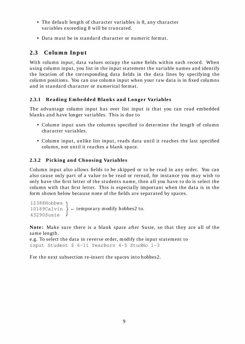
Column input also allows fields to be skipped or to be read in any order. You canalso cause only part of a value to be read or reread, for instance you may wish toonly have the first letter of the students name, then all you have to do is select thecolumn with that first letter. This is especially important when the data is in theform shown below because none of the fields are separated by spaces.

12388Hobbes10189Calvin43290Susie

9=; ← temporary modify hobbes2 to.

Note: Make sure there is a blank space after Susie, so that they are all of thesame length.e.g. To select the data in reverse order, modify the input statement toinput Student $ 6-11 YearBorn 4-5 StudNo 1-3

For the next subsection re-insert the spaces into hobbes2.

9

2.4 Combining List and Column Inputs

Now that we have included the students names we may wish to exclude the studentnumber, this we can do by modifying the input line to

input YearBorn 5-6 Student $;

Where 5-6 refers to the columns where your first desired variable is. The ommi-sion of any further column references informs SAS that each subsequent variable inthe input statement will correspond to the subsequent variable in the data file.Suppose you just wanted the student number and their name but not their age thenyou would need to modify the input statement as follows

input StudNo Student $ 8-13;

Where 8-13 refers to the columns where the student names are. The dollar signcan be on either side of the column reference.Note: this assumes that all the data is properly set up in columns, because if forexample you had the following

123 88 Hobbes 123 88101 89 Calvin 101 89432 90 Susie 432 90

You can see that the columns method would fail after Susie because the “4” orthe “432” would fall in the wrong column in which case you would have to use thelist input.

2.5 Data Files with Different Formats

For brevity I have not shown you every possible format for data set which SAS canhandle but should you wish to explore more refer to one of the SAS manual whichare available at the computer services library.

2.6 Impossible Data Files

Occasionally you may get an impossible data file such as

12388Hobbes1238810189Calvin1018943290Susie43290

In such cases you will have to edit the data file first.

10

2.7 Creating Dependent Variables

Sometimes you will wish to create variables which depend on existing ones, for ex-ample you may wish to know the actual ages of the students according to the currentyear minus their date of birth. You can do this by inserting behind the input state-ment

libname calvin ’susie’;data calvin.ageclub;infile ’hobbes2’;input StudNo YearBorn Student $;StudAge=97-YearBorn;

run;proc print data=calvin.ageclub;run;

For reference the addition operators are as follows

• addition +

• subtraction -

• multiplication *

• division /

• power **

2.7.1 Logic Statements

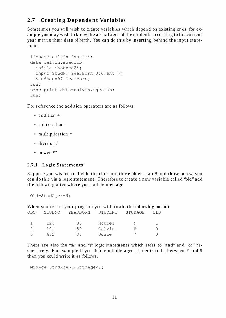
Suppose you wished to divide the club into those older than 8 and those below, youcan do this via a logic statement. Therefore to create a new variable called “old” addthe following after where you had defined age

Old=StudAge>=9;

When you re-run your program you will obtain the following output.OBS STUDNO YEARBORN STUDENT STUDAGE OLD

1 123 88 Hobbes 9 12 101 89 Calvin 8 03 432 90 Susie 7 0

There are also the “&” and “” logic statements which refer to “and” and “or” re-spectively. For example if you define middle aged students to be between 7 and 9then you could write it as follows.

MidAge=StudAge>7&StudAge<9;

11

For reference here is the full set of relation operators

Symbol Mnemonic Operator Meaning= EQ equal to

˜ = NE not equal to> GT greater than< LT less than

>= GE greater than or equal to<= LE less than or equal to

2.8 Use of “If” Statements

Suppose you wished to divide the ages further into the categories young, middleaged and old. This can be done via an “if” statement as follows

libname calvin ’susie’;data calvin.ageclub;infile ’hobbes2’;input StudNo YearBorn Student $;StudAge=97-YearBorn;if StudAge>=9 then AgeCat=’Senior’;else if StudAge=8 then AgeCat=’Middle Aged’;else AgeCat=’Child’;

run;proc print data=calvin.ageclub;run;

Note: The “if” does not require an “end” statement.Submitting the above program gives you the output

Age of Club Members 1109:08 Tuesday, October 1, 1996

OBS STUDNO YEARBORN STUDENT STUDAGE AGECAT

1 123 88 Hobbes 9 Senior2 101 89 Calvin 8 Middle3 432 90 Susie 7 Child

Notice how AgeCat got truncated to the length of its first item. You can specify thelength you require via a “length” statement, to modify the previous one, you caninsert a length statement as follows.

StudAge=97-YearBorn;length AgeCat $ 11;if StudAge>=9 then AgeCat=’Old’;

12

You also use “and” and “or” statements. For instance the “and” statement works asfollows

if StudAge>7 & StudAge<9 then MidAged=’Yes’;else MidAged=’No ’;

or similarly

if 7<StudAge<9 then MidAged=’Yes’;else MidAged=’No ’;

Similarly the “or” statement works as follows

if StudAge<=7 | StudAge>=9 then MidAged=’No ’;else MidAged=’Yes’;

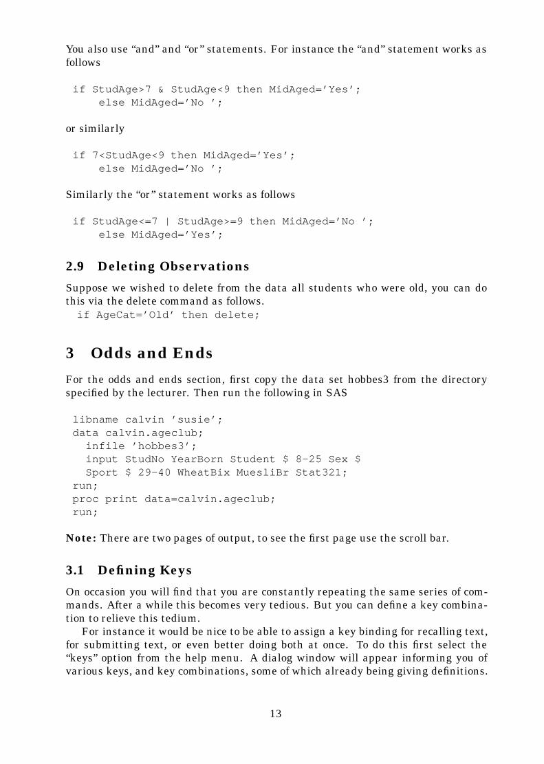
2.9 Deleting Observations

Suppose we wished to delete from the data all students who were old, you can dothis via the delete command as follows.if AgeCat=’Old’ then delete;

3 Odds and Ends

For the odds and ends section, first copy the data set hobbes3 from the directoryspecified by the lecturer. Then run the following in SAS

libname calvin ’susie’;data calvin.ageclub;infile ’hobbes3’;input StudNo YearBorn Student $ 8-25 Sex $Sport $ 29-40 WheatBix MuesliBr Stat321;

run;proc print data=calvin.ageclub;run;

Note: There are two pages of output, to see the first page use the scroll bar.

3.1 Defining Keys

On occasion you will find that you are constantly repeating the same series of com-mands. After a while this becomes very tedious. But you can define a key combina-tion to relieve this tedium.

For instance it would be nice to be able to assign a key binding for recalling text,for submitting text, or even better doing both at once. To do this first select the“keys” option from the help menu. A dialog window will appear informing you ofvarious keys, and key combinations, some of which already being giving definitions.

13

Note: The definitions linked with the keys F1-F12 will not work as they have alreadybeen assigned for system use, e.g. F1 iconises the window. Shift-F1 to Shift-F12 canbe defined but be careful when defining shift-F10 because should you forget the shiftcomponent you will destroy your window. The KP keys all work except the "KP ,"which doesn’t exist, but for some of them such as KP 0 (the Ins key) you must alsouse the shift. All the control(Ctrl) keys also work.

Now suppose you wished to define CTRL A to be the key which will recall thelast program and then submit it. To do this click next to Ctrl A and type

pgm; recall; submit

Note: pgm is short for program manager(editor).Now select save from the File menu to store the key binding.

3.2 Including Comments within your SAS Program

To include comments in your SAS programs all you need to do is insert a /∗ at thestart of your comment and a ∗/ at the end of your comment. e.g./* This is a sample comment */

3.3 Sorting your Data

SAS’s Sort procedure has the form of the addition to hobbes1 below

proc sort data=calvin.ageclub out=sortclub;by YearBorn;

run;proc print calvin.sortclub; /* Prints sorted data */run;

Note: If you are not using permanent data sets, you may omit references to datasets.

3.3.1 Sorting by more than one Variable

You can sort by more than one variable by including the additional variables inthe by statement. For instance if you wished to sort also by the variables Sex andWheatbix then you would modify as follows.

proc sort data=calvin.ageclub out=sortclub;by Sex Wheatbix;

run;proc print;run;

Note: As sortclub was the last data set created, “proc print”, selects it as thedefault.

14

3.3.2 Sorting in Descending Order

To sort a variable in descending order you only need to modify the program as follows

proc sort data=calvin.ageclub out=sortclub;by descending YearBorn;

run;proc print;run;

3.3.3 Removing Duplicates

The “Noduplicates” option in the sort procedure deletes any observation that dupli-cates the values of all variables of another observation in the data set. For instanceLucy van Pelt appears twice in the data set, so to remove the duplication write thefollowing

proc sort data=calvin.ageclub out=calvin.ageclubnoduplicates;by YearBorn;

run;proc print;run;

3.4 Using the Inbuilt Help Facility

In general the inbuilt help facility is useless or frustrating. But with items like thesort procedure their help is handy as a reminder of the syntax and options. To findhelp on “sort”, you need to do the following.

• Select “Extended Help” from the “Help” menu. (A new window will appear).

• Click on “Data Management”.

• Click on “Sort”.

• Click on “Introduction”.

• After reading the introduction, click on “GoBack”.

• Click on “Syntax”.

You can click on any bold text and you will get a brief explanation of that topic, usethe “GoBack” command to go back to the previous screen. Once you feel that youhave explored the “sort” procedure sufficiently click on GoBack repeatedly until youhave exited help. Do not just click on “exit help”, unless you wish your next helpquery to start where you left off.

15

3.5 Using the Means Procedure

Instead of having a series of procedures for calculating minimums, maximums etc,they have all been combined into the proc means procedure where you can selectwhich statistical information you require from the available options. For a list ofthese options and the syntax, use the extended help as follows

• Click on “Modeling and Analysis Tools”.

• Click on “Data Analysis”.

• Click on “Means”.

• Click on topics of interest. e.g Click on Syntax, then options.

• Once finished click on GoBack until you exit help.

3.6 Calculating Correlations and Covariances

These can be calculated by using the correlation procedure (the covariance portionis one of the suboptions). Help on its use can be found with the online help underModeling & Analysis Tools → Data Analysis → corr.Note: unlike previous procedures this procedure does send output to the SAS:OUTPUT window, and therefore an additional print procedure is not needed.e.g.proc means data=calvin.ageclub n min max;class Sex;

run;

4 SAS Graphics

SAS has two styles of graphics, low level graphics consisting of ASCIIcharacters, and high level graphics.

4.1 Low Level Graphics (Scatter Plots)

An example of a simple plot of YearBorn vs WheatBix is

proc plot data=calvin.ageclub;plot WheatBix*YearBorn;

run;

Where WheatBix is along the vertical axis and YearBorn is along the horizontal.By default, the Plot procedure

• Prints the name of the vertical variable next to the vertical axis and the nameof the horizontal variable beneath the horizontal axis.

• Chooses ranges for both axes and automatically places tick marks at reasonablyspaced intervals.

16

• Uses the letter A as the plotting symbol to indicate one observation; the letterB if two observations coincide; and so on.

• Prints a legend naming the variables in the plot and explaining the plottingsymbols.

4.1.1 Adding Title and Labels to a Plot

proc plot data=calvin.ageclub;plot WheatBix*YearBorn;title ’Plot of WheatBix versus Year of Birth’;label WheatBix=’WheatBix Eating’

YearBorn=’Year of Birth’;run;

4.1.2 Modifying Tickmarks

proc plot data=calvin.ageclub;plot WheatBix*YearBorn / vaxis=0 to 10 by 2;

run;

This will modify the vertical axis to start at 0 and then going up in steps of 2up to 10. You can similarly modify the horizontal axis using “haxis”.

4.1.3 Specifying Plotting Symbols

Should you wish to specify the “asterisk (*)” as the plotting symbol, you simply dothe following

proc plot data=calvin.ageclub;plot WheatBix*YearBorn=’*’;

run;

Note: When you specify a plotting symbol, proc plot uses that symbol for all pointson the plot regardless of how many observations may coincide. If observations docoincide, a message appears at the bottom of the plot telling you how many observa-tions are hidden.

4.1.4 Creating Multiple Plots

Rather than do separate plots for different variables, they can be combined as followsproc plot data=calvin.ageclub;

plot WheatBix*YearBorn=’*’ MuesliBr*YearBorn=’o’;run;

4.1.5 Creating Multiple Plots on the Same Page

To help make it easier to compare graphs you can do multiple plots on the same“page” (by page I refer to a SAS page) via “vpercent” and “hpercent”. Using thevpercent you have the following

17

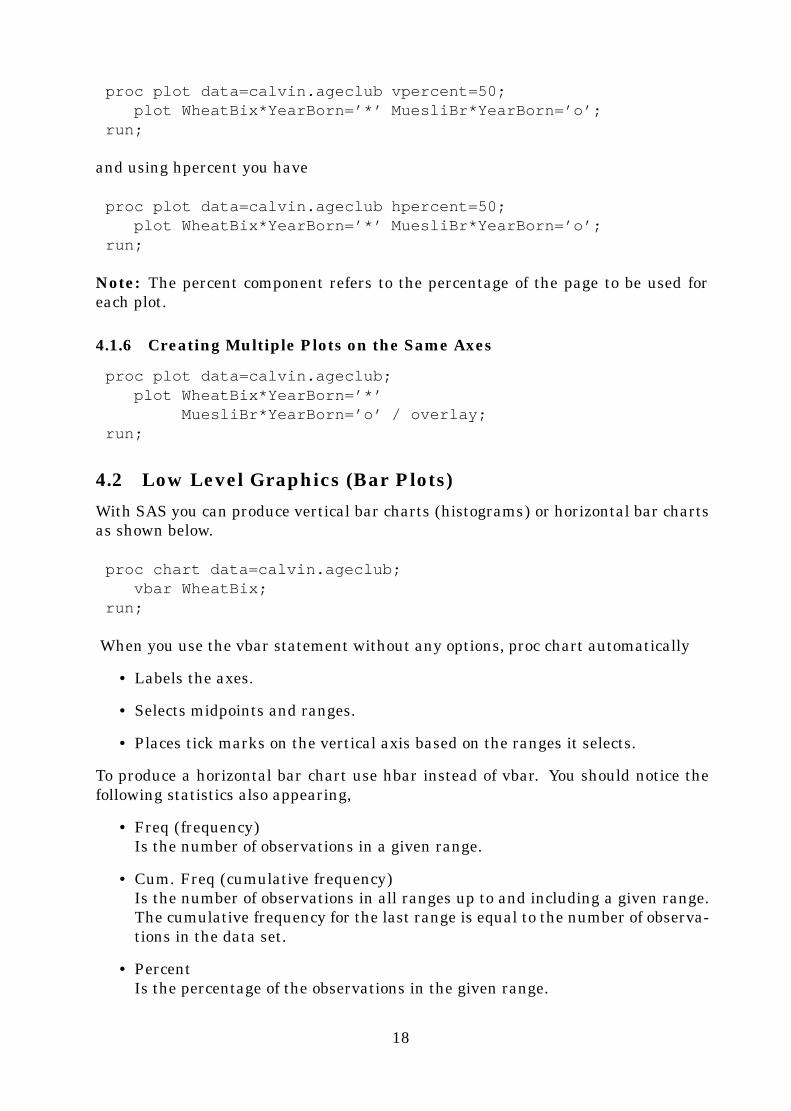
proc plot data=calvin.ageclub vpercent=50;plot WheatBix*YearBorn=’*’ MuesliBr*YearBorn=’o’;

run;

and using hpercent you have

proc plot data=calvin.ageclub hpercent=50;plot WheatBix*YearBorn=’*’ MuesliBr*YearBorn=’o’;

run;

Note: The percent component refers to the percentage of the page to be used foreach plot.

4.1.6 Creating Multiple Plots on the Same Axes

proc plot data=calvin.ageclub;plot WheatBix*YearBorn=’*’

MuesliBr*YearBorn=’o’ / overlay;run;

4.2 Low Level Graphics (Bar Plots)

With SAS you can produce vertical bar charts (histograms) or horizontal bar chartsas shown below.

proc chart data=calvin.ageclub;vbar WheatBix;

run;

When you use the vbar statement without any options, proc chart automatically

• Labels the axes.

• Selects midpoints and ranges.

• Places tick marks on the vertical axis based on the ranges it selects.

To produce a horizontal bar chart use hbar instead of vbar. You should notice thefollowing statistics also appearing,

• Freq (frequency)Is the number of observations in a given range.

• Cum. Freq (cumulative frequency)Is the number of observations in all ranges up to and including a given range.The cumulative frequency for the last range is equal to the number of observa-tions in the data set.

• PercentIs the percentage of the observations in the given range.

18

• Cum. Percent (Cumulative percent)Is the percentage of observations in all ranges up to and including a givenrange. The cumulative percentage for the last range is always 100.

To eliminate these statistics modify your SAS program to

proc chart data=calvin.ageclub;hbar WheatBix / nostat;

run;

4.2.1 Specifying Midpoint Values

You can specify midpoints as follows

proc chart data=calvin.ageclub;vbar Stat321 / midpoints=10 to 90 by 20;

run;

The corresponding ranges are

0 to 1920 to 3940 to 5960 to 7980 to 99

4.2.2 Specifying Number of Midpoints

You can specify the number of midpoints by using the levels statement as follows

proc chart data=calvin.ageclub;vbar Stat321 / levels=5;

run;

4.2.3 Charting every Value

Should you wish to have a bar of every value, one can use the discrete option asfollows

proc chart data=calvin.ageclub;vbar WheatBix / discrete;

run;

19

4.2.4 Creating Subgroups within a Range

To split WheatBix consumption within the bars by gender you can use the followingSAS statements.

proc chart data=calvin.ageclub;vbar WheatBix / subgroup=sex;

run;

4.2.5 Grouping Bars

To split WheatBix consumption into separate bar charts according gender you canuse the following SAS statements.

proc chart data=calvin.ageclub;vbar Stat321 / group=sex;

run;

5 High Level Graphics

5.1 Scatter Plots

A simple example of a scatter plot is

proc gplot data=calvin.ageclub;plot WheatBix*YearBorn;

run;

Notice that the only difference between this and the low level graphics is the gplotstatement.

5.1.1 Adding a Title

You can add a title using the command “title”e.g. title ’Plot of WheatBix versus Year of Birth’;Note: To view subsequent graphs press the PgDn key, and to view previous graphspress the PgUp key.The title command has several options which are as follows

• Positiontitle move=(-1cm,-1cm)

’Plot of WheatBix versus Year of Birth’;

• Sizetitle height=0.5cm

’Plot of WheatBix versus Year of Birth’;

• Fonttitle font=brush’Plot of WheatBix versus Year of Birth’;

20

• Mix Fontstitle font=brush ’Plot of ’ font=cscript ’’WheatBix ’ font=brush ’versus ’font=cscript ’Year of Birth’;

• Multiple titlestitle font=brush’Plot of WheatBix versus Year of Birth’;title2 font=cscript ’For the Club’;

Note: one can have up to ten titles, numbered 1-10, e.g title5.For more details of titles and other graphic options consult the online help.

5.2 Bar Plots

Firstly start off looking at a simple histogram

proc gchart data=calvin.ageclub;vbar sport;title font=brush ’Histogram of Sports’;

run;

You will notice that each of the bars are solid blocks. While this looks nice onthe screen, when printing it is very wasteful of printer ink, not to mention slower.One can use the pattern subcommand to define another pattern style, an exampleshowing its use will be given later. See the “extended help” for exact details.

5.2.1 Bar Plots with Subgroups

Supposing you want to produce a bar chart with subgroups, you could do that asfollows

proc gchart data=calvin.ageclub;vbar sport / subgroup=sex;title font=brush ’Histogram of Sports by Sex’;

run;

You will notice that SAS automatically assigns a pattern for each gender and thenincludes a legend (key), informing you of which pattern it has assigned to whichgender. You can similarly define your own as shown in the following example

proc gchart data=calvin.ageclub;vbar sport / subgroup=sex;title font=brush ’Histogram of Sports by Sex’;pattern1 value=L1;pattern2 value=X1;

run;

21

5.3 Pie Charts

Here is a simple example of a pie chart

proc gchart data=calvin.ageclub;pie sport/ NOHEADING value=noneslice=arrow PERCENT=none;title font=brush ’List of Sports’;pattern1 value=p3n0;pattern2 value=p3n45;pattern3 value=p3n90;pattern4 value=p3n135;pattern5 value=p3x0;

run;

5.4 Graphic Options

Whenever you produce a graph in which you define some graphic options, these op-tions will also exist for future graphs within your session, unless modified. In somesituations you may wish to know what graphic options you have already defined, todo this, you will use the goptions procedure as follows

proc goptions;run;

Examining the SAS: LOG window will give you an alphabetic list of options with adescription and present values.Note: there is also a goptions statement which you can use to define graphic options.For instance to include the graphics options for the previous pie chart you wouldproceed as follows.

goptions;title font=brush ’List of Sports’;pattern1 value=p3x0;pattern2 value=p3n90;pattern3 value=p3n135;pattern4 value=p3n45;pattern5 value=p3n0;/* Note: goptions does not require a run statement.*/proc gchart data=calvin.ageclub;

pie sport/ NOHEADING value=noneslice=arrow PERCENT=none;

run;

22

5.5 Printing Graphs

To print your graphs on the laser printer, you proceed with

filename gsasfile ’snoopy.ps’;goptions device=ps300 gaccess=gsasfile;proc gchart data=calvin.ageclub;

pie sport;run;

The filename statement has the syntax

filename fileref ’external-file’;

You replace fileref with a SAS name of no more than eight letters, in this caseit must be called “gsasfile”. You replace external-file with the name you wish to callyour graph. Your filename can be of any length but you are advised to include a .psextension so that you can easily identify it as a postscript file in the future.Note: Once you have defined a SAS name to be a file, you cannot redefine the nameas something else until you have quit out of the prior name.For example

quit;filename gsasfile ’kermit.ps’;goptions device=ps300 gaccess=gsasfile;proc gchart data=calvin.ageclub;

pie sport;run;

Where the quit statement at the beginning cancels out the earlier reference tosnoopy.ps. You will have noticed that your graphs are not appearing on the screenbut are being sent only to a file. The next subsection will inform you of how to viewyour graphs on the screen again.

5.6 Graphics to file → graphics to screen

To return to having graphics on your screen specify the device to be empty.i.e.goptions device=’’;proc gchart data=calvin.ageclub;

pie sport;run;

23

6 Exercises

1. Create a simple program which creates a temporary data set called butterflywith the numerical variables “acre” and “transline”. Insert into your programthe first three rows of data for acre and transline as shown in the appendix.Submit your program in SAS, then before you hand it in examine the logwindow to ensure that your program contains no errors. For future exercisesyou may be required to use this program, hence you are advised to store thisprogram in your directory.

2. Modify the program from ex 1 to include a print procedure, submit your pro-gram and save the output to a file.

3. Create a permanent data set of the data set using all 26 values of the datausing all of the variables as shown in the appendix. To save time, you maywish to copy the file from the “/users/math/underg/sas” directory into your ownarea.

4. Create a new program designed to obtain a subset of the data set created inexercise 3 such that it only contains the last ten observations.

5. Add to your program from exercise 3 the string variable “ageclass”.

6. Create a subset of the data so that only data for ageclasses being young areselected.

7. Write a sas formula for converting the area in acres to meters and save it asthe new variable msq.

8. Create a new string variable called size, such that

(a) If acre < 25, size is small

(b) If 25 ≤ acre < 50, size is medium

(c) If 50 ≤ acre < 100, size is large

(d) If acre ≥ 100, size is xtlarge

Once finished compare with classsize and make sure that they are the same.

9. Remove all data that has classsize as extra large.

10. Add a comment to your program

11. Sort your data according to acre in reverse order. How have the classsizes beengrouped?

12. Using the help facility find out how to use anova and impliment with the modelkbb=acre.

13. Plot acre by kbb using a “o” as the plotting symbol

14. Create a vbar chart of kbb with midpoints ranging from 0 to 50 in steps of 10by the variable ageclass.

15. Create a pie chart of ageclass.

24

7 Appendix

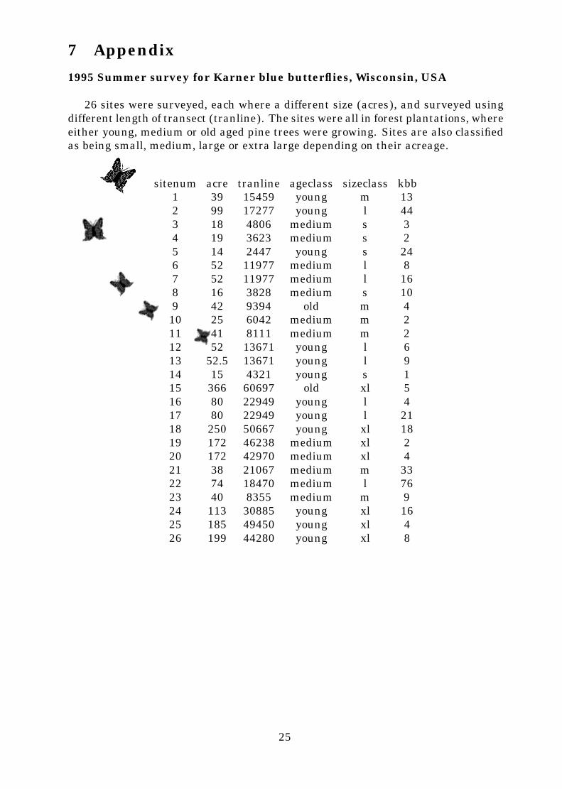
1995 Summer survey for Karner blue butterflies, Wisconsin, USA

26 sites were surveyed, each where a different size (acres), and surveyed usingdifferent length of transect (tranline). The sites were all in forest plantations, whereeither young, medium or old aged pine trees were growing. Sites are also classifiedas being small, medium, large or extra large depending on their acreage.

sitenum acre tranline ageclass sizeclass kbb1 39 15459 young m 132 99 17277 young l 443 18 4806 medium s 34 19 3623 medium s 25 14 2447 young s 246 52 11977 medium l 87 52 11977 medium l 168 16 3828 medium s 109 42 9394 old m 4

10 25 6042 medium m 211 41 8111 medium m 212 52 13671 young l 613 52.5 13671 young l 914 15 4321 young s 115 366 60697 old xl 516 80 22949 young l 417 80 22949 young l 2118 250 50667 young xl 1819 172 46238 medium xl 220 172 42970 medium xl 421 38 21067 medium m 3322 74 18470 medium l 7623 40 8355 medium m 924 113 30885 young xl 1625 185 49450 young xl 426 199 44280 young xl 8

25

Index$, 8

Bar Plots, High Level, 21Bar Plots, Low Level, 18

Cards, 2Character Variables, 8Column Input, 9, 10Comments, 14Correlation, 16Covariance, 16

Data Set, Temporary, 2Data Sets, 6Deleting Observations, 13Duplicates, 15

Editing, 1Exit, 2

Formats, 10

Gcharts, 21Goptions, 22Graph, Title, 20Graphics, High Level, 20Graphics, Low Level, 16Graphs, Label, 17Graphs, Printing, 23Graphs, Title, 17

Hbar, 19Help, 15Hpercent, 18

If, 12Information, 15Input, 2Inputting Data, 8

Keys, 13

Label, 17Libname, 6List Input, 8, 10Loading Data, 5Log, 2, 4Logic Statements, 11

Means Procedure, 16

Midpoints, 19Multiple Plots, 18Multiple Plots, 17

Output, 2

Page Size, 5Pie Charts, 22Plotting Symbols, 17Printing to Printer, 5Printing, Graphs, 23Program Editor, 1, 2, 4

Quit, 2

Relation Operators, 12Running, 3

Sas Names, 1Saving Data, 6Saving Output, 6Scatter Plots, High Level, 20Scatter Plots, Low Level, 16Screen Output, 4, 5Selecting, 7, 9Session, 2Short Cuts, 4Sort, Descending, 15Sort, Multivariables, 14Sorting, 14Statements, Rules, 3Subgroups, 20Submit, 3Subsets, 7

Tab, 2Title, 17

Variables, Dependent, 11Vbar, 18Vpercent, 18

26