INTRODUCTORY COMPUTER

NETWORKSPHYSICAL LAYER, DIGITAL TRANSMISSION

FUNDAMENTALS

FaramarzHendessi

2

Lecture 8Fall 2010

Isfahan University of technology

Dr. Faramarz Hendessi

Introductory Computer

Networks

3

DIGITAL TRANSMISSION

FUNDAMENTALS

Properties of Media and Digital Transmission Systems

Lecture 8

Fall 2009

4

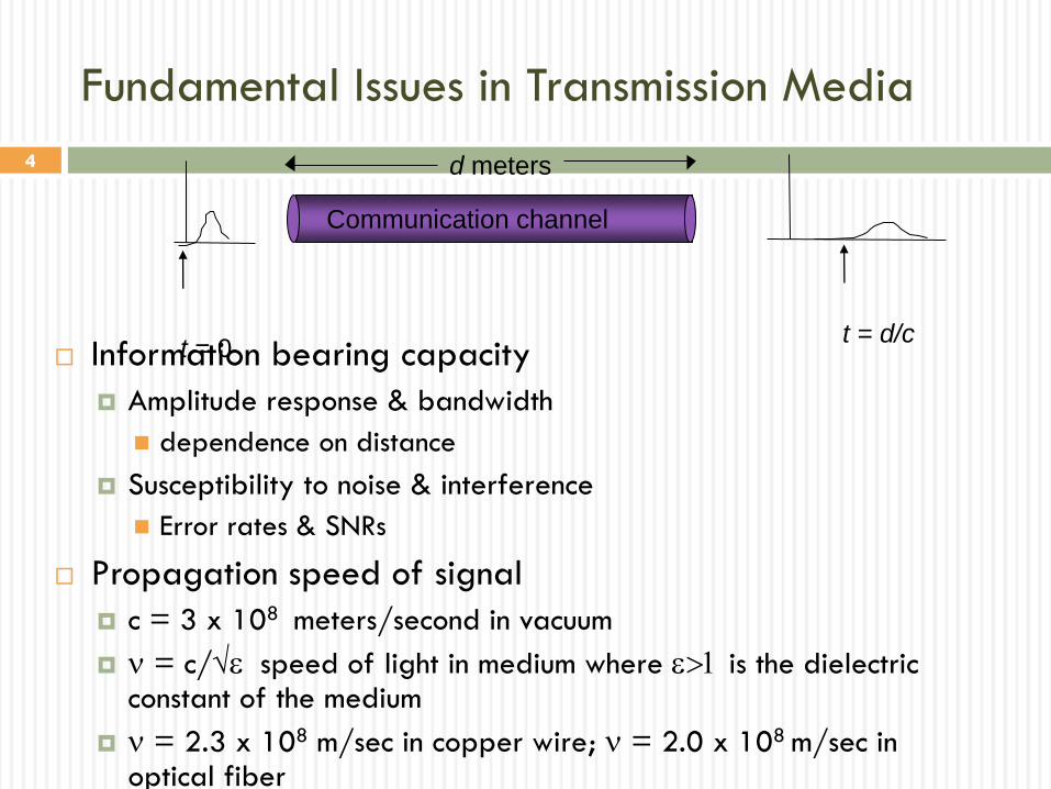
Fundamental Issues in Transmission Media

Information bearing capacity

Amplitude response & bandwidth

dependence on distance

Susceptibility to noise & interference

Error rates & SNRs

Propagation speed of signal

c = 3 x 108 meters/second in vacuum

= c/√e speed of light in medium where e>1 is the dielectric constant of the medium

= 2.3 x 108 m/sec in copper wire; = 2.0 x 108 m/sec in optical fiber

t = 0t = d/c

Communication channel

d meters

5

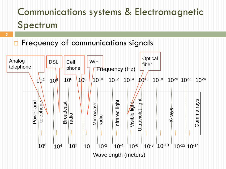
Communications systems & Electromagnetic

Spectrum

Frequency of communications signals

Analog

telephoneDSL Cell

phone

WiFiOptical

fiber

102 104 106 108 1010 1012 1014 1016 1018 1020 1022 1024

Frequency (Hz)

Wavelength (meters)

106 104 102 10 10-2 10-4 10-6 10-8 10-10 10-12 10-14

Po

we

r a

nd

tele

ph

on

e

Bro

ad

ca

st

radio

Mic

row

ave

radio

Infr

are

d lig

ht

Vis

ible

lig

ht

Ultra

vio

let lig

ht

X-r

ays

Ga

mm

a r

ays

6

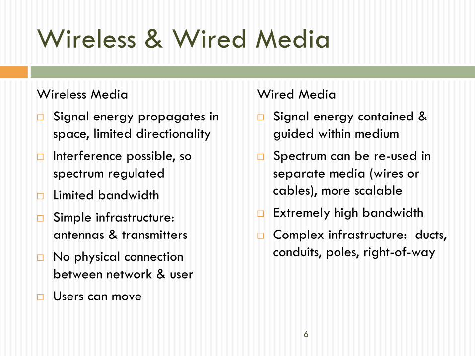
Wireless & Wired Media

Wireless Media

Signal energy propagates in

space, limited directionality

Interference possible, so

spectrum regulated

Limited bandwidth

Simple infrastructure:

antennas & transmitters

No physical connection

between network & user

Users can move

Wired Media

Signal energy contained &

guided within medium

Spectrum can be re-used in

separate media (wires or

cables), more scalable

Extremely high bandwidth

Complex infrastructure: ducts,

conduits, poles, right-of-way

7

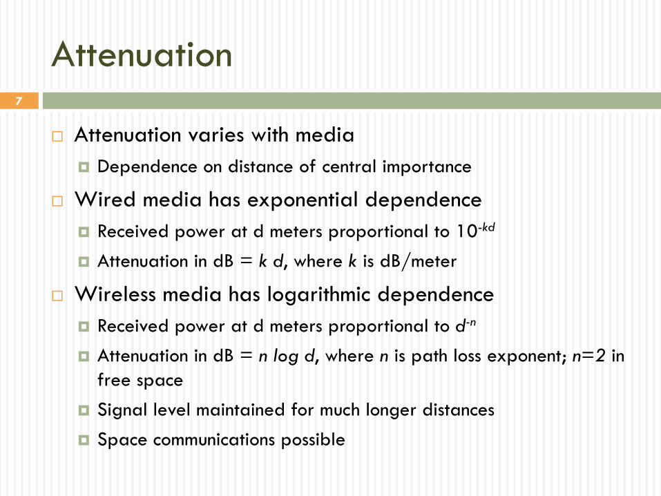
Attenuation

Attenuation varies with media

Dependence on distance of central importance

Wired media has exponential dependence

Received power at d meters proportional to 10-kd

Attenuation in dB = k d, where k is dB/meter

Wireless media has logarithmic dependence

Received power at d meters proportional to d-n

Attenuation in dB = n log d, where n is path loss exponent; n=2 in

free space

Signal level maintained for much longer distances

Space communications possible

8

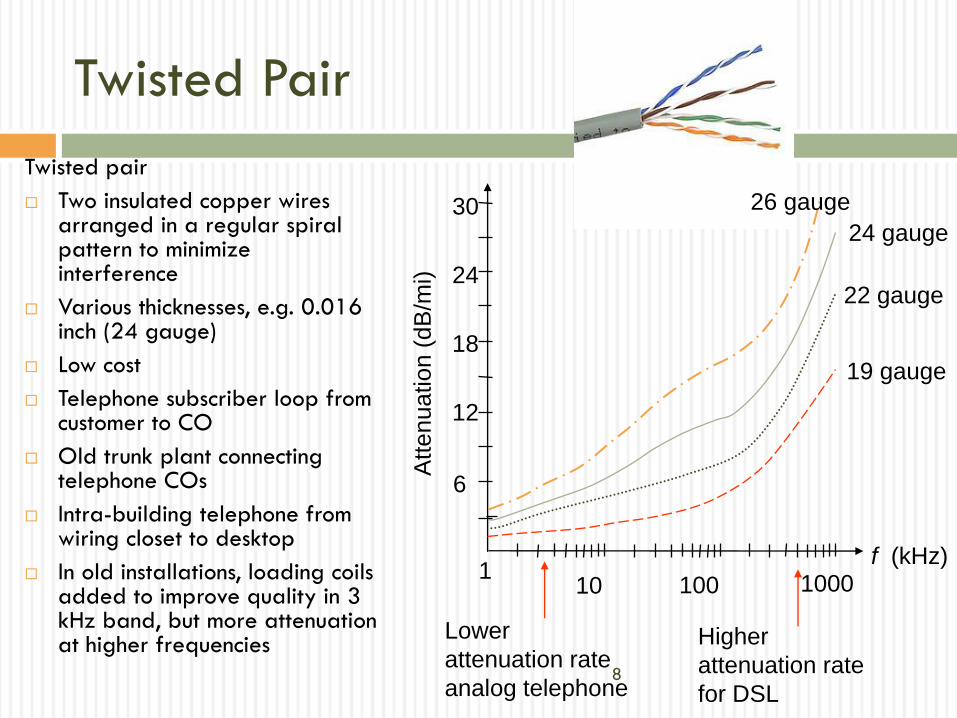
Twisted Pair

Twisted pair

Two insulated copper wires arranged in a regular spiral pattern to minimize interference

Various thicknesses, e.g. 0.016 inch (24 gauge)

Low cost

Telephone subscriber loop from customer to CO

Old trunk plant connecting telephone COs

Intra-building telephone from wiring closet to desktop

In old installations, loading coils added to improve quality in 3 kHz band, but more attenuation at higher frequencies

Atten

ua

tio

n (

dB

/mi)

f (kHz)

19 gauge

22 gauge

24 gauge

26 gauge

6

12

18

24

30

110 100 1000

Lower

attenuation rate

analog telephone

Higher

attenuation rate

for DSL

9

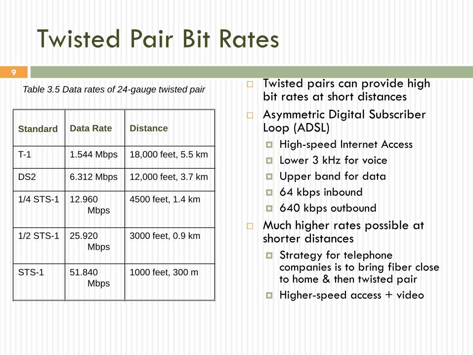
Twisted Pair Bit Rates

Twisted pairs can provide high bit rates at short distances

Asymmetric Digital Subscriber Loop (ADSL)

High-speed Internet Access

Lower 3 kHz for voice

Upper band for data

64 kbps inbound

640 kbps outbound

Much higher rates possible at shorter distances

Strategy for telephone companies is to bring fiber close to home & then twisted pair

Higher-speed access + video

Table 3.5 Data rates of 24-gauge twisted pair

Standard Data Rate Distance

T-1 1.544 Mbps 18,000 feet, 5.5 km

DS2 6.312 Mbps 12,000 feet, 3.7 km

1/4 STS-1 12.960

Mbps

4500 feet, 1.4 km

1/2 STS-1 25.920

Mbps

3000 feet, 0.9 km

STS-1 51.840

Mbps

1000 feet, 300 m

10

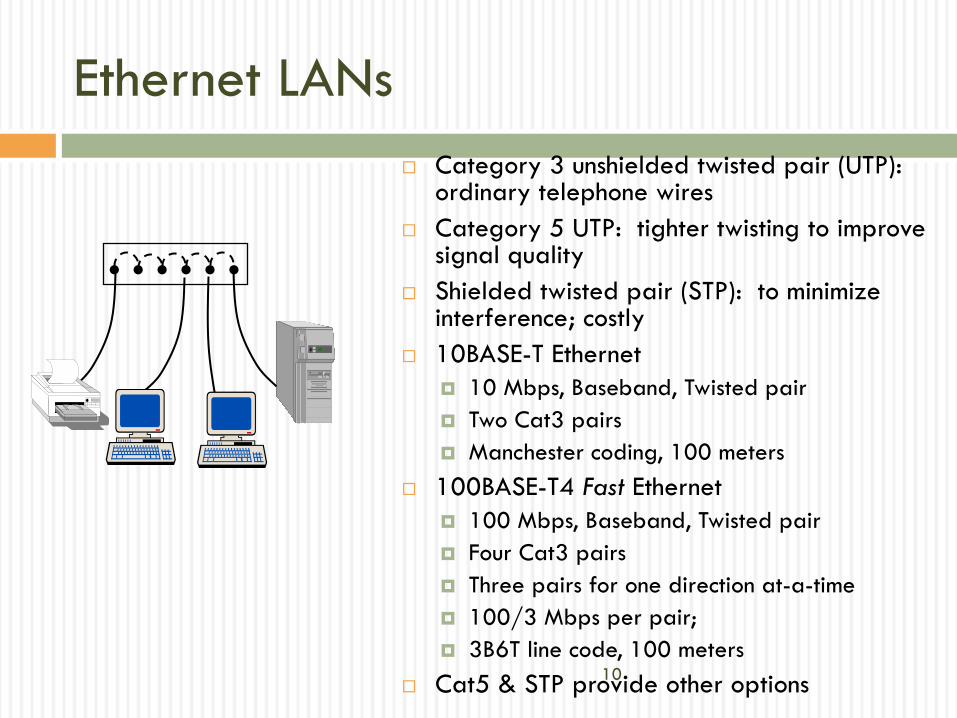
Ethernet LANs

Category 3 unshielded twisted pair (UTP): ordinary telephone wires

Category 5 UTP: tighter twisting to improve signal quality

Shielded twisted pair (STP): to minimize interference; costly

10BASE-T Ethernet

10 Mbps, Baseband, Twisted pair

Two Cat3 pairs

Manchester coding, 100 meters

100BASE-T4 Fast Ethernet

100 Mbps, Baseband, Twisted pair

Four Cat3 pairs

Three pairs for one direction at-a-time

100/3 Mbps per pair;

3B6T line code, 100 meters

Cat5 & STP provide other options

11

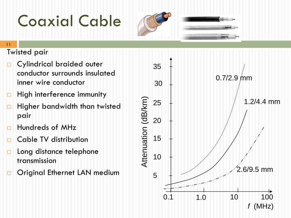
Coaxial Cable

Twisted pair

Cylindrical braided outer conductor surrounds insulated inner wire conductor

High interference immunity

Higher bandwidth than twisted pair

Hundreds of MHz

Cable TV distribution

Long distance telephone transmission

Original Ethernet LAN medium

35

30

10

25

20

5

15A

ttenuation (

dB

/km

)

0.1 1.0 10 100

f (MHz)

2.6/9.5 mm

1.2/4.4 mm

0.7/2.9 mm

12

UpstreamDownstream

5 M

Hz

42

MH

z

54

MH

z

50

0 M

Hz

55

0 M

Hz

75

0

MH

z

Downstream

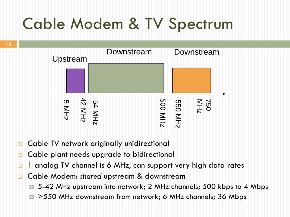
Cable Modem & TV Spectrum

Cable TV network originally unidirectional

Cable plant needs upgrade to bidirectional

1 analog TV channel is 6 MHz, can support very high data rates

Cable Modem: shared upstream & downstream

5-42 MHz upstream into network; 2 MHz channels; 500 kbps to 4 Mbps

>550 MHz downstream from network; 6 MHz channels; 36 Mbps

13

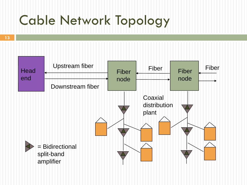
Cable Network Topology

Head

end

Upstream fiber

Downstream fiber

Fiber

node

Coaxial

distribution

plant

Fiber

node

= Bidirectional

split-band

amplifier

Fiber Fiber

14

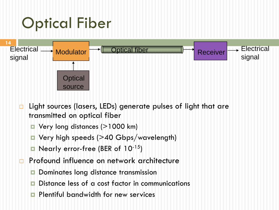
Optical Fiber

Light sources (lasers, LEDs) generate pulses of light that are transmitted on optical fiber

Very long distances (>1000 km)

Very high speeds (>40 Gbps/wavelength)

Nearly error-free (BER of 10-15)

Profound influence on network architecture

Dominates long distance transmission

Distance less of a cost factor in communications

Plentiful bandwidth for new services

Optical fiber

Optical

source

ModulatorElectrical

signalReceiver

Electrical

signal

15

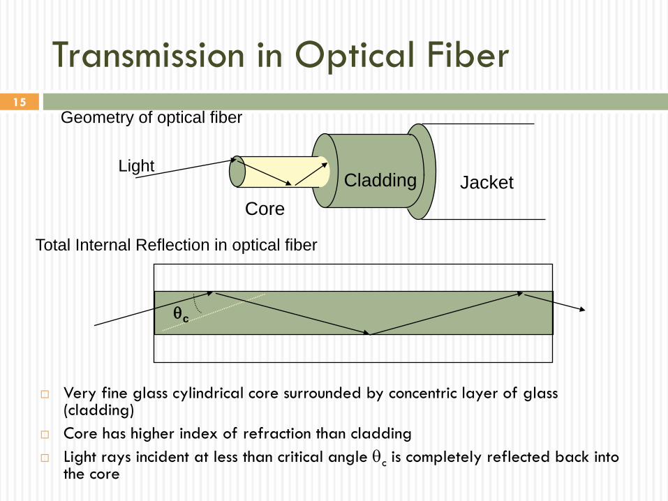
Core

Cladding JacketLight

c

Geometry of optical fiber

Total Internal Reflection in optical fiber

Transmission in Optical Fiber

Very fine glass cylindrical core surrounded by concentric layer of glass (cladding)

Core has higher index of refraction than cladding

Light rays incident at less than critical angle c is completely reflected back into the core

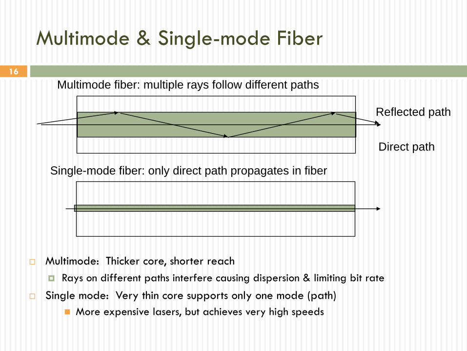
16

Multimode: Thicker core, shorter reach

Rays on different paths interfere causing dispersion & limiting bit rate

Single mode: Very thin core supports only one mode (path)

More expensive lasers, but achieves very high speeds

Multimode fiber: multiple rays follow different paths

Single-mode fiber: only direct path propagates in fiber

Direct path

Reflected path

Multimode & Single-mode Fiber

17

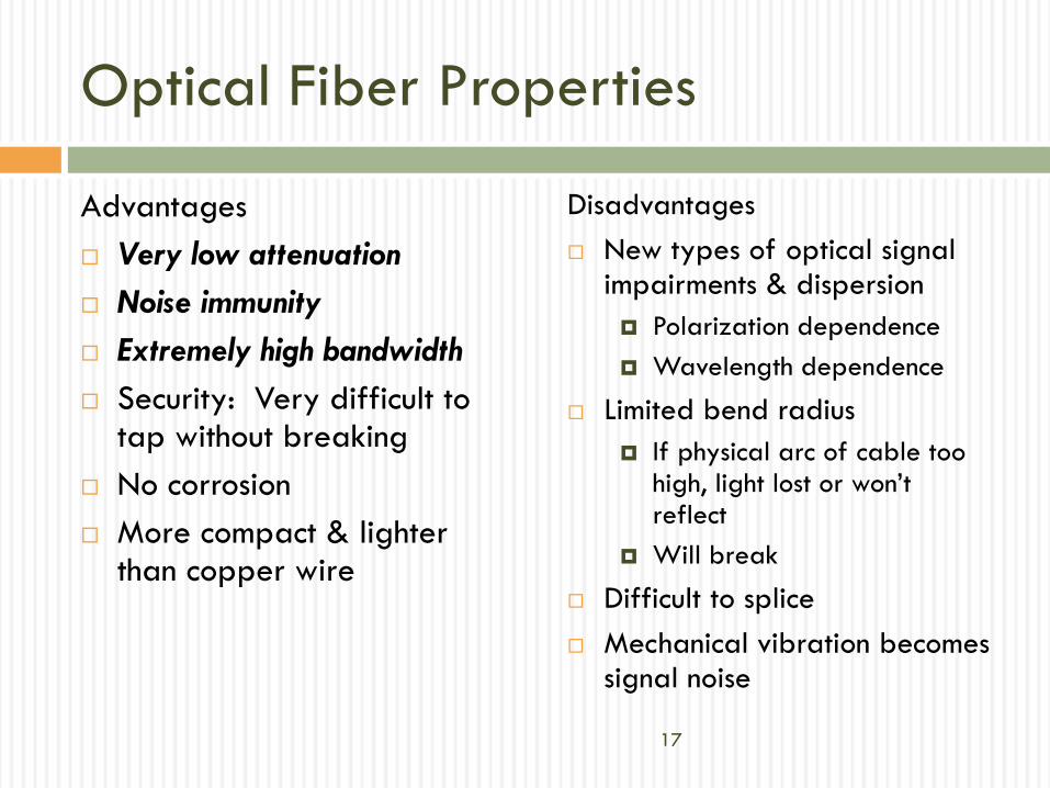
Optical Fiber Properties

Advantages

Very low attenuation

Noise immunity

Extremely high bandwidth

Security: Very difficult to tap without breaking

No corrosion

More compact & lighter than copper wire

Disadvantages

New types of optical signal impairments & dispersion

Polarization dependence

Wavelength dependence

Limited bend radius

If physical arc of cable too high, light lost or won‟t reflect

Will break

Difficult to splice

Mechanical vibration becomes signal noise

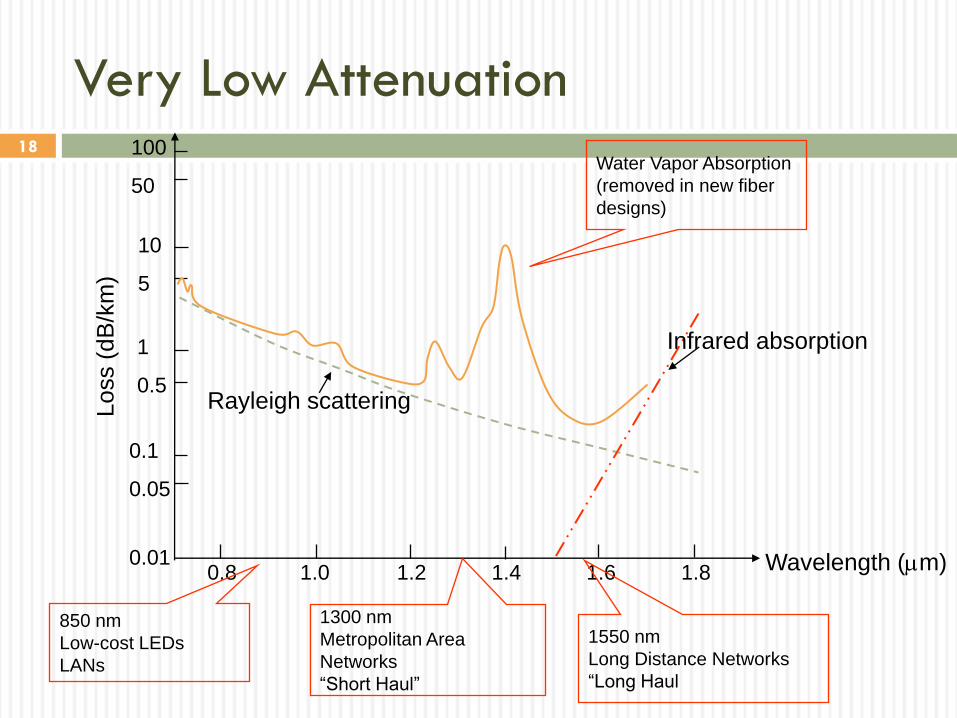
18 100

50

10

5

1

0.5

0.1

0.05

0.010.8 1.0 1.2 1.4 1.6 1.8 Wavelength (m)

Loss (

dB

/km

)

Infrared absorption

Rayleigh scattering

Very Low Attenuation

850 nm

Low-cost LEDs

LANs

1300 nm

Metropolitan Area

Networks

“Short Haul”

1550 nm

Long Distance Networks

“Long Haul

Water Vapor Absorption

(removed in new fiber

designs)

19

100

50

10

5

1

0.5

0.1

0.8 1.0 1.2 1.4 1.6 1.8

Loss (

dB

/km

)

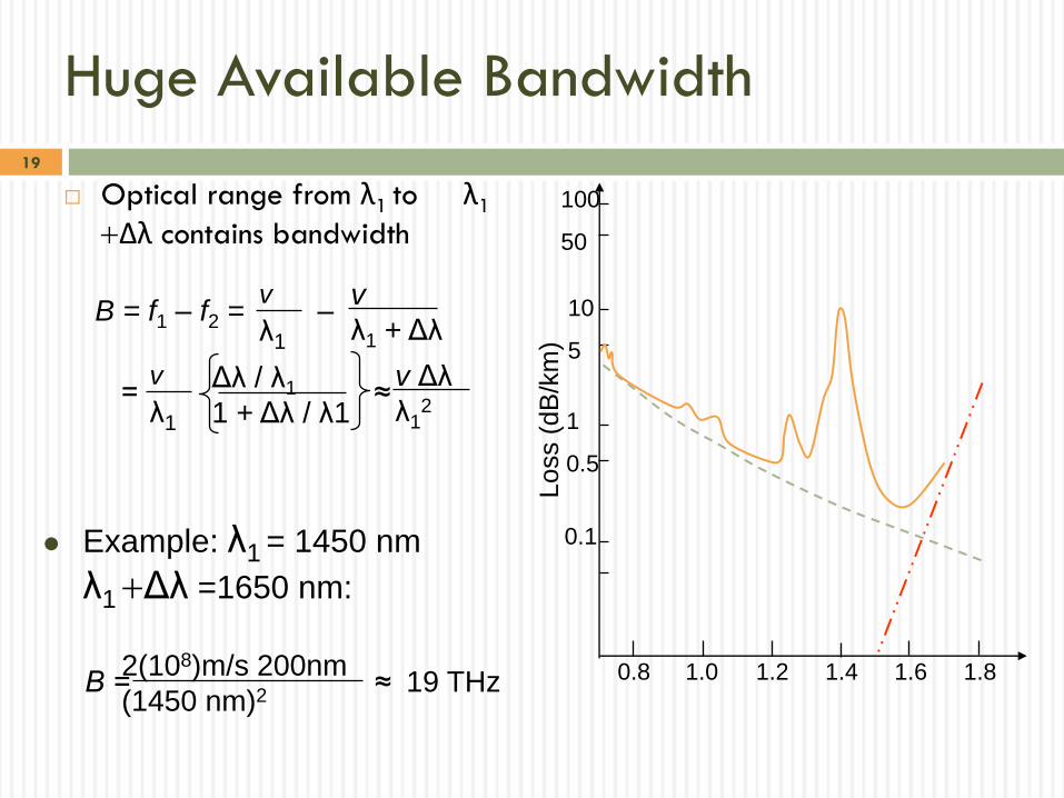
Huge Available Bandwidth

Optical range from λ1 to λ1

+Δλ contains bandwidth

Example: λ1 = 1450 nm

λ1 +Δλ =1650 nm:

B = ≈ 19 THz

B = f1 – f2 = –v

λ1 + Δλ

v

λ1

v Δλ

λ12

= ≈ Δλ / λ1

1 + Δλ / λ1

v

λ1

2(108)m/s 200nm

(1450 nm)2

20

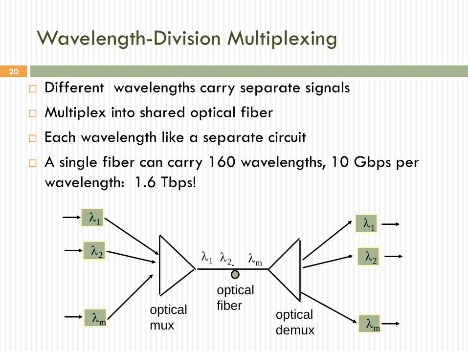
Wavelength-Division Multiplexing

Different wavelengths carry separate signals

Multiplex into shared optical fiber

Each wavelength like a separate circuit

A single fiber can carry 160 wavelengths, 10 Gbps per

wavelength: 1.6 Tbps!

1

2

m

optical

mux

1

2

m

optical

demux

1 2. m

optical

fiber

21

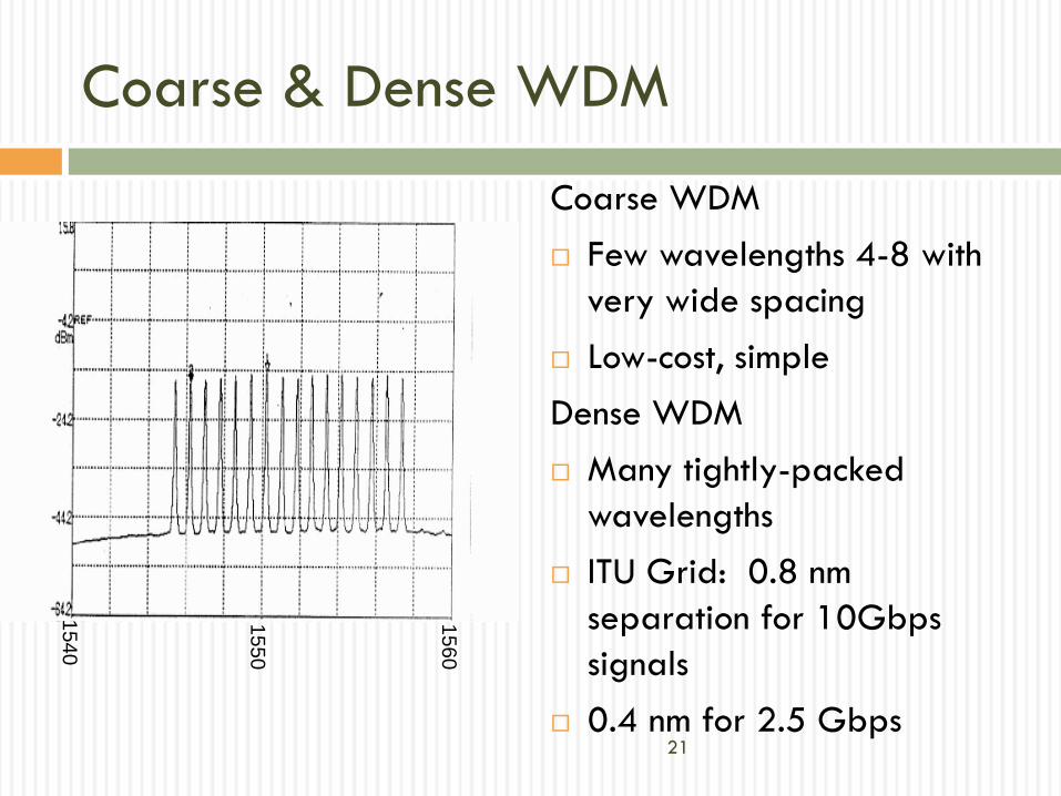
Coarse & Dense WDM

Coarse WDM

Few wavelengths 4-8 with

very wide spacing

Low-cost, simple

Dense WDM

Many tightly-packed

wavelengths

ITU Grid: 0.8 nm

separation for 10Gbps

signals

0.4 nm for 2.5 Gbps

15

50

15

60

15

40

22

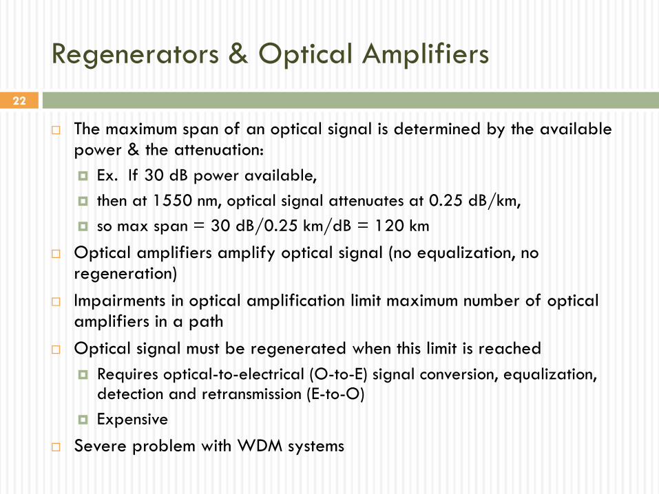
Regenerators & Optical Amplifiers

The maximum span of an optical signal is determined by the available power & the attenuation:

Ex. If 30 dB power available,

then at 1550 nm, optical signal attenuates at 0.25 dB/km,

so max span = 30 dB/0.25 km/dB = 120 km

Optical amplifiers amplify optical signal (no equalization, no regeneration)

Impairments in optical amplification limit maximum number of optical amplifiers in a path

Optical signal must be regenerated when this limit is reached

Requires optical-to-electrical (O-to-E) signal conversion, equalization, detection and retransmission (E-to-O)

Expensive

Severe problem with WDM systems

23

Regenerator

R R R R R R R R

DWDM

multiplexer

… …R

R

R

R

…R

R

R

R

…R

R

R

R

…R

R

R

R…

DWDM & Regeneration

Single signal per fiber requires 1 regenerator per span

DWDM system carries many signals in one fiber

At each span, a separate regenerator required per signal

Very expensive

24

R

R

R

R

Optical

amplifier

… … …R

R

R

R

OA OA OA OA… …

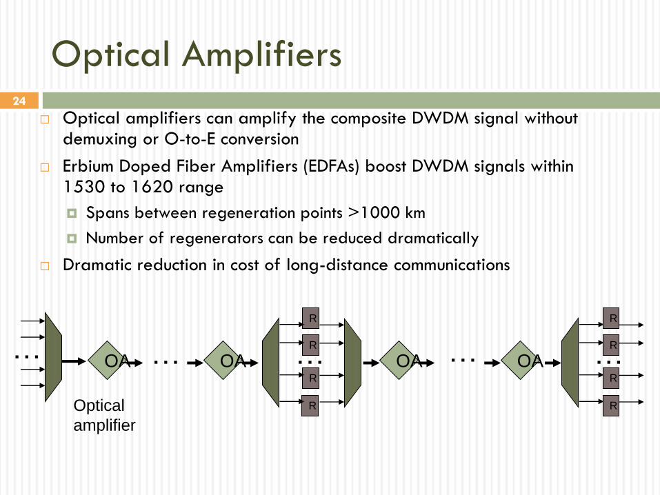
Optical Amplifiers

Optical amplifiers can amplify the composite DWDM signal without demuxing or O-to-E conversion

Erbium Doped Fiber Amplifiers (EDFAs) boost DWDM signals within 1530 to 1620 range

Spans between regeneration points >1000 km

Number of regenerators can be reduced dramatically

Dramatic reduction in cost of long-distance communications

25

Radio Transmission

Radio signals: antenna transmits sinusoidal signal

(“carrier”) that radiates in air/space

Information embedded in carrier signal using modulation,

e.g. QAM

Communications without tethering

Cellular phones, satellite transmissions, Wireless LANs

Multipath propagation causes fading

Interference from other users

Spectrum regulated by national & international

regulatory organizations

26

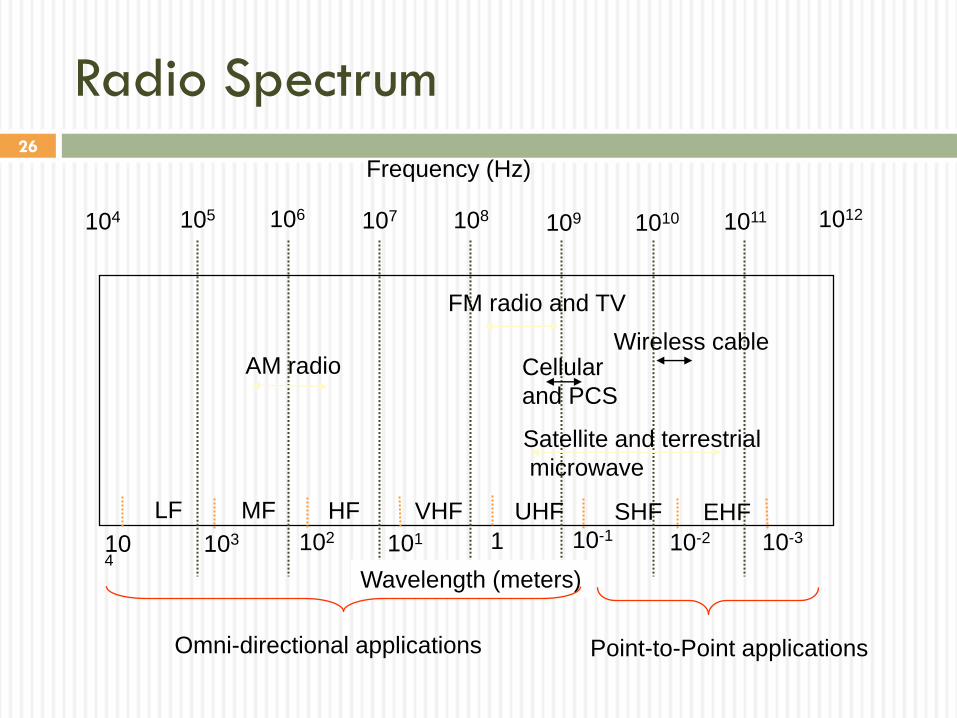
104 106 107 108 109 1010 1011 1012

Frequency (Hz)

Wavelength (meters)

103 102 101 1 10-1 10-2 10-3

105

Satellite and terrestrial

microwave

AM radio

FM radio and TV

LF MF HF VHF UHF SHF EHF

104

Cellular

and PCS

Wireless cable

Radio Spectrum

Omni-directional applications Point-to-Point applications

27

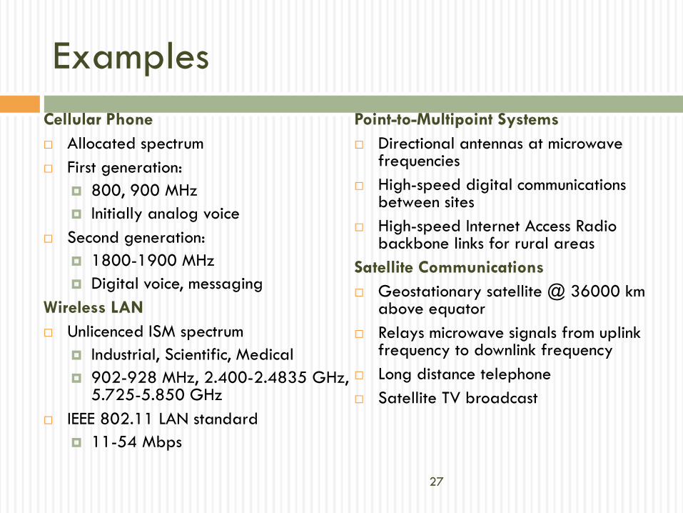
Examples

Cellular Phone

Allocated spectrum

First generation:

800, 900 MHz

Initially analog voice

Second generation:

1800-1900 MHz

Digital voice, messaging

Wireless LAN

Unlicenced ISM spectrum

Industrial, Scientific, Medical

902-928 MHz, 2.400-2.4835 GHz, 5.725-5.850 GHz

IEEE 802.11 LAN standard

11-54 Mbps

Point-to-Multipoint Systems

Directional antennas at microwave frequencies

High-speed digital communications between sites

High-speed Internet Access Radio backbone links for rural areas

Satellite Communications

Geostationary satellite @ 36000 km above equator

Relays microwave signals from uplink frequency to downlink frequency

Long distance telephone

Satellite TV broadcast

28

PHYSICAL LAYER:

Error Detection and Correction

RS-232 Asynchronous Data Transmission

Lecture 9

Fall 2009

29

DIGITAL TRANSMISSION

FUNDAMENTALS

Error Detection and Correction

Lecture 9

Fall 2009

30

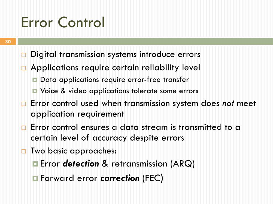
Error Control

Digital transmission systems introduce errors

Applications require certain reliability level

Data applications require error-free transfer

Voice & video applications tolerate some errors

Error control used when transmission system does not meet application requirement

Error control ensures a data stream is transmitted to a certain level of accuracy despite errors

Two basic approaches:

Error detection & retransmission (ARQ)

Forward error correction (FEC)

31

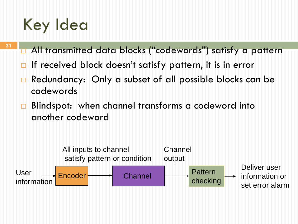
Key Idea

All transmitted data blocks (“codewords”) satisfy a pattern

If received block doesn‟t satisfy pattern, it is in error

Redundancy: Only a subset of all possible blocks can be codewords

Blindspot: when channel transforms a codeword into another codeword

ChannelEncoderUser

information

Pattern

checking

All inputs to channel

satisfy pattern or condition

Channel

output

Deliver user

information or

set error alarm

32

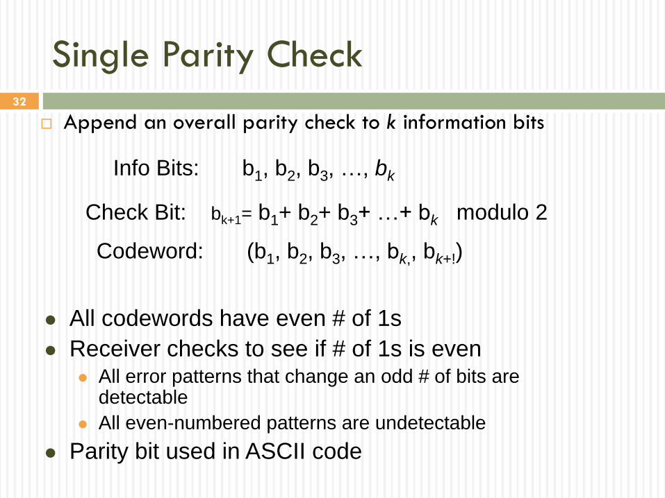
Single Parity Check

Append an overall parity check to k information bits

Info Bits: b1, b2, b3, …, bk

Check Bit: bk+1= b1+ b2+ b3+ …+ bk modulo 2

Codeword: (b1, b2, b3, …, bk,, bk+!)

All codewords have even # of 1s

Receiver checks to see if # of 1s is even All error patterns that change an odd # of bits are

detectable

All even-numbered patterns are undetectable

Parity bit used in ASCII code

33

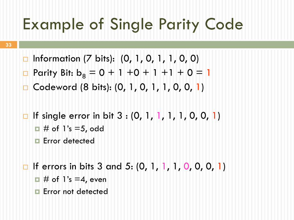
Example of Single Parity Code

Information (7 bits): (0, 1, 0, 1, 1, 0, 0)

Parity Bit: b8 = 0 + 1 +0 + 1 +1 + 0 = 1

Codeword (8 bits): (0, 1, 0, 1, 1, 0, 0, 1)

If single error in bit 3 : (0, 1, 1, 1, 1, 0, 0, 1)

# of 1‟s =5, odd

Error detected

If errors in bits 3 and 5: (0, 1, 1, 1, 0, 0, 0, 1)

# of 1‟s =4, even

Error not detected

34

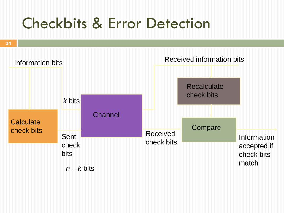
Checkbits & Error Detection

Calculate

check bits

Channel

Recalculate

check bits

Compare

Information bitsReceived information bits

Sent

check

bits

Information

accepted if

check bits

match

Received

check bits

k bits

n – k bits

35

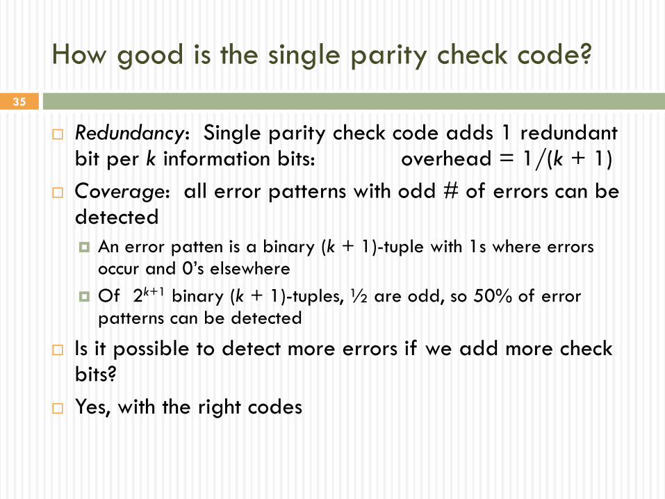
How good is the single parity check code?

Redundancy: Single parity check code adds 1 redundant bit per k information bits: overhead = 1/(k + 1)

Coverage: all error patterns with odd # of errors can be detected

An error patten is a binary (k + 1)-tuple with 1s where errors occur and 0‟s elsewhere

Of 2k+1 binary (k + 1)-tuples, ½ are odd, so 50% of error patterns can be detected

Is it possible to detect more errors if we add more check bits?

Yes, with the right codes

36

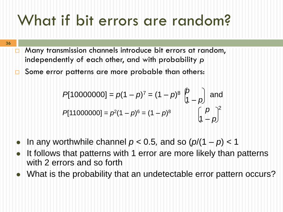
What if bit errors are random?

Many transmission channels introduce bit errors at random, independently of each other, and with probability p

Some error patterns are more probable than others:

In any worthwhile channel p < 0.5, and so (p/(1 – p) < 1

It follows that patterns with 1 error are more likely than patterns with 2 errors and so forth

What is the probability that an undetectable error pattern occurs?

P[10000000] = p(1 – p)7 = (1 – p)8 and

P[11000000] = p2(1 – p)6 = (1 – p)8

p

1 – p

p 2

1 – p

37

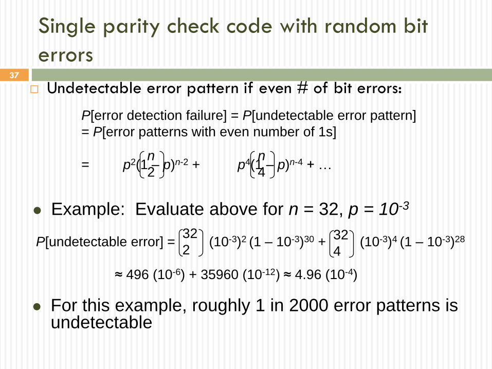
Single parity check code with random bit

errors

Undetectable error pattern if even # of bit errors:

Example: Evaluate above for n = 32, p = 10-3

For this example, roughly 1 in 2000 error patterns is undetectable

P[error detection failure] = P[undetectable error pattern]

= P[error patterns with even number of 1s]

= p2(1 – p)n-2 + p4(1 – p)n-4 + …n

2

n

4

P[undetectable error] = (10-3)2 (1 – 10-3)30 + (10-3)4 (1 – 10-3)28

≈ 496 (10-6) + 35960 (10-12) ≈ 4.96 (10-4)

32

232

4

38

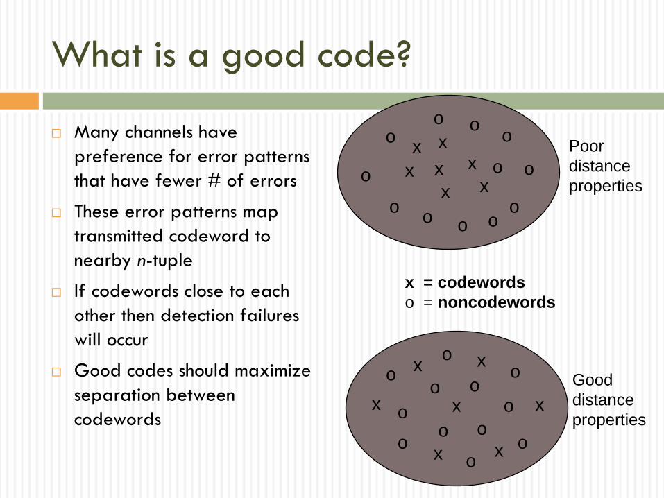
x = codewords

o = noncodewords

x

x x

x

x

x

x

o

oo

oo

oo

o

oo

o

o

o

x

x x

x

xx

x

oo

oo

oooo

o

o

oPoor

distance

properties

What is a good code?

Many channels have

preference for error patterns

that have fewer # of errors

These error patterns map

transmitted codeword to

nearby n-tuple

If codewords close to each

other then detection failures

will occur

Good codes should maximize

separation between

codewords

Good

distance

properties

39

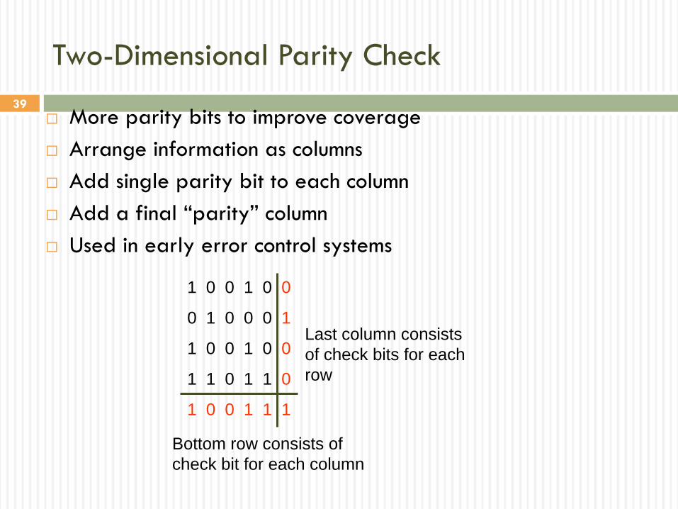
Two-Dimensional Parity Check

1 0 0 1 0 0

0 1 0 0 0 1

1 0 0 1 0 0

1 1 0 1 1 0

1 0 0 1 1 1

Bottom row consists of

check bit for each column

Last column consists

of check bits for each

row

More parity bits to improve coverage

Arrange information as columns

Add single parity bit to each column

Add a final “parity” column

Used in early error control systems

40

1 0 0 1 0 0

0 0 0 1 0 1

1 0 0 1 0 0

1 0 0 0 1 0

1 0 0 1 1 1

1 0 0 1 0 0

0 0 0 0 0 1

1 0 0 1 0 0

1 0 0 1 1 0

1 0 0 1 1 1

1 0 0 1 0 0

0 0 0 1 0 1

1 0 0 1 0 0

1 0 0 1 1 0

1 0 0 1 1 1

1 0 0 1 0 0

0 0 0 0 0 1

1 0 0 1 0 0

1 1 0 1 1 0

1 0 0 1 1 1

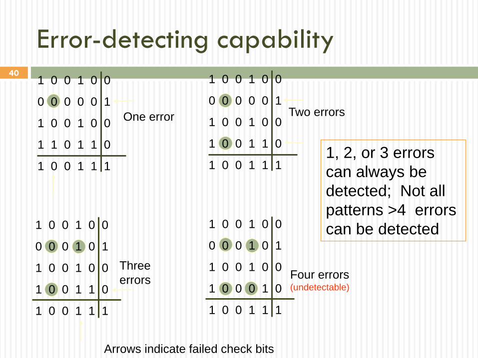
Arrows indicate failed check bits

Two errorsOne error

Three

errors Four errors (undetectable)

Error-detecting capability

1, 2, or 3 errors

can always be

detected; Not all

patterns >4 errors

can be detected

41

Other Error Detection Codes

Many applications require very low error rate

Need codes that detect the vast majority of errors

Single parity check codes do not detect enough errors

Two-dimensional codes require too many check bits

The following error detecting codes used in practice:

Internet Check Sums

CRC Polynomial Codes

42

Internet Checksum

Several Internet protocols (e.g. IP, TCP, UDP) use check bits

to detect errors in the IP header (or in the header and data

for TCP/UDP)

A checksum is calculated for header contents and included in

a special field.

Checksum recalculated at every router, so algorithm selected

for ease of implementation in software

Let header consist of L, 16-bit words,

b0, b1, b2, ..., bL-1

The algorithm appends a 16-bit checksum bL

43

The checksum bL is calculated as follows:

Treating each 16-bit word as an integer, find

x = b0 + b1 + b2+ ...+ bL-1 modulo 216-1

The checksum is then given by:

bL = - x modulo 216-1

Thus, the headers must satisfy the following pattern:

0 = b0 + b1 + b2+ ...+ bL-1 + bL modulo 216-1

The checksum calculation is carried out in software using one‟s

complement arithmetic

Checksum Calculation

44

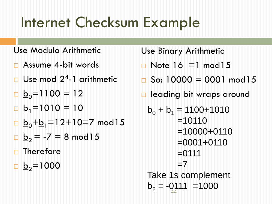
Internet Checksum Example

Use Modulo Arithmetic

Assume 4-bit words

Use mod 24-1 arithmetic

b0=1100 = 12

b1=1010 = 10

b0+b1=12+10=7 mod15

b2 = -7 = 8 mod15

Therefore

b2=1000

Use Binary Arithmetic

Note 16 =1 mod15

So: 10000 = 0001 mod15

leading bit wraps around

b0 + b1 = 1100+1010

=10110

=10000+0110

=0001+0110

=0111

=7

Take 1s complement

b2 = -0111 =1000

45

Polynomial Codes

Polynomials instead of vectors for codewords

Polynomial arithmetic instead of check sums

Implemented using shift-register circuits

Also called cyclic redundancy check (CRC) codes

Most data communications standards use

polynomial codes for error detection

Polynomial codes also basis for powerful error-

correction methods

46

Addition:

Multiplication:

Binary Polynomial Arithmetic

Binary vectors map to polynomials

(ik-1 , ik-2 ,…, i2 , i1 , i0) ik-1xk-1 + ik-2x

k-2 + … + i2x2 + i1x + i0

(x7 + x6 + 1) + (x6 + x5) = x7 + x6 + x6 + x5 + 1

= x7 +(1+1)x6 + x5 + 1

= x7 +x5 + 1 since 1+1=0 mod2

(x + 1) (x2 + x + 1) = x(x2 + x + 1) + 1(x2 + x + 1)

= x3 + x2 + x) + (x2 + x + 1)

= x3 + 1

47

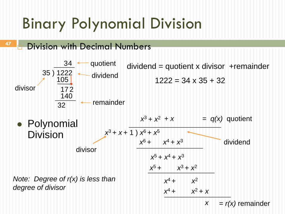
Binary Polynomial Division

Division with Decimal Numbers

32

35 ) 1222

3

105

17 2

4

140divisor

quotient

remainder

dividend1222 = 34 x 35 + 32

dividend = quotient x divisor +remainder

Polynomial Division x3 + x + 1 ) x6 + x5

x6 + x4 + x3

x5 + x4 + x3

x5 + x3 + x2

x4 + x2

x4 + x2 + x

x

= q(x) quotient

= r(x) remainder

divisordividend

+ x+ x2x3

Note: Degree of r(x) is less than

degree of divisor

48

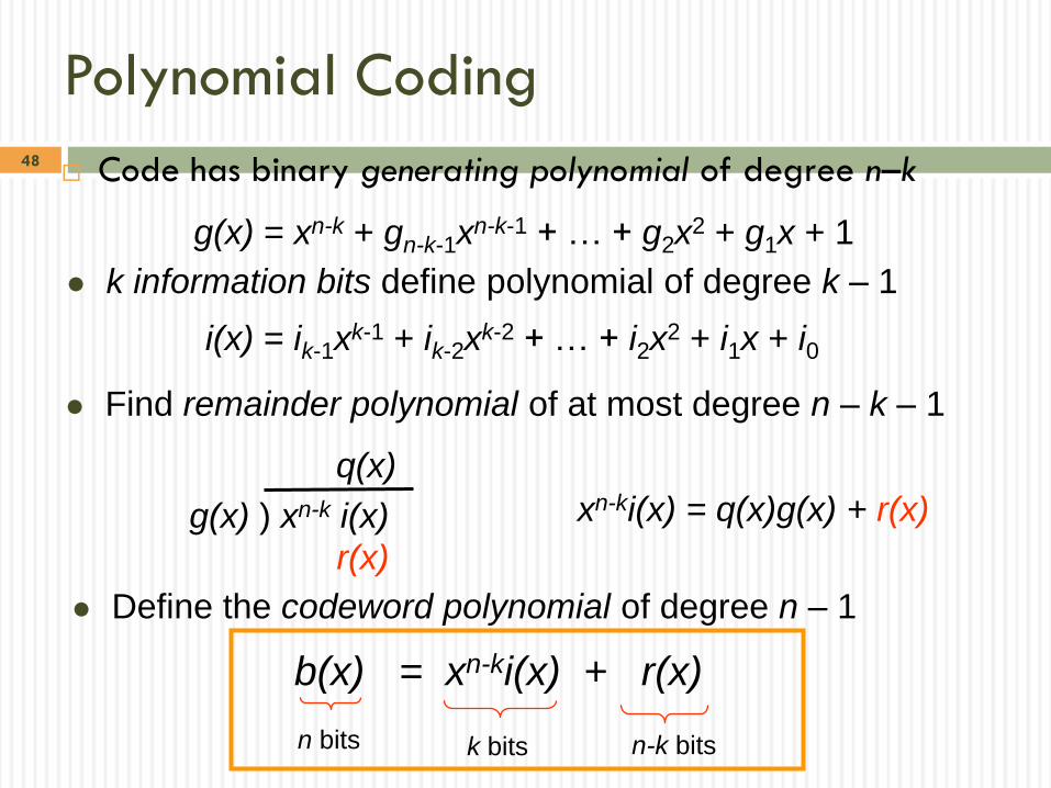
Polynomial Coding

Code has binary generating polynomial of degree n–k

k information bits define polynomial of degree k – 1

Find remainder polynomial of at most degree n – k – 1

g(x) ) xn-k i(x)

q(x)

r(x)

xn-ki(x) = q(x)g(x) + r(x)

Define the codeword polynomial of degree n – 1

b(x) = xn-ki(x) + r(x)

n bits k bits n-k bits

g(x) = xn-k + gn-k-1xn-k-1 + … + g2x

2 + g1x + 1

i(x) = ik-1xk-1 + ik-2x

k-2 + … + i2x2 + i1x + i0

49

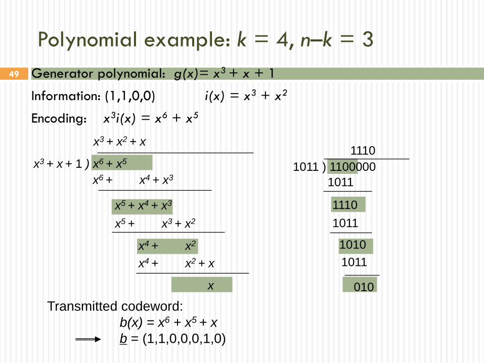
Transmitted codeword:

b(x) = x6 + x5 + x

b = (1,1,0,0,0,1,0)

1011 ) 1100000

1110

1011

1110

1011

1010

1011

010

x3 + x + 1 ) x6 + x5

x3 + x2 + x

x6 + x4 + x3

x5 + x4 + x3

x5 + x3 + x2

x4 + x2

x4 + x2 + x

x

Polynomial example: k = 4, n–k = 3

Generator polynomial: g(x)= x3 + x + 1

Information: (1,1,0,0) i(x) = x3 + x2

Encoding: x3i(x) = x6 + x5

50

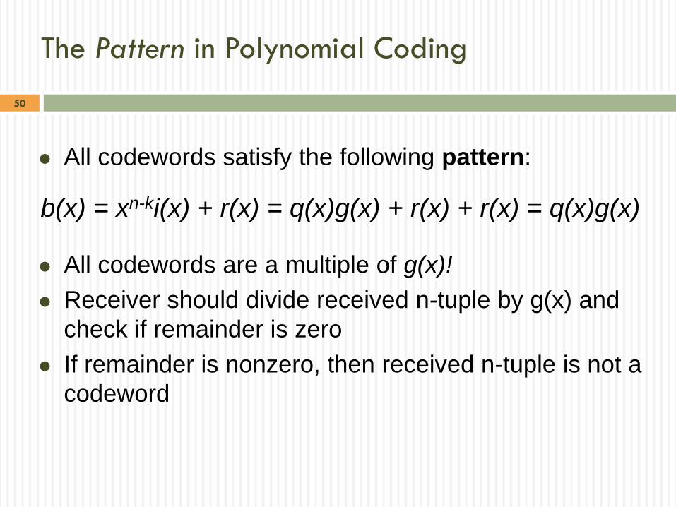
The Pattern in Polynomial Coding

All codewords satisfy the following pattern:

All codewords are a multiple of g(x)!

Receiver should divide received n-tuple by g(x) and

check if remainder is zero

If remainder is nonzero, then received n-tuple is not a

codeword

b(x) = xn-ki(x) + r(x) = q(x)g(x) + r(x) + r(x) = q(x)g(x)

51

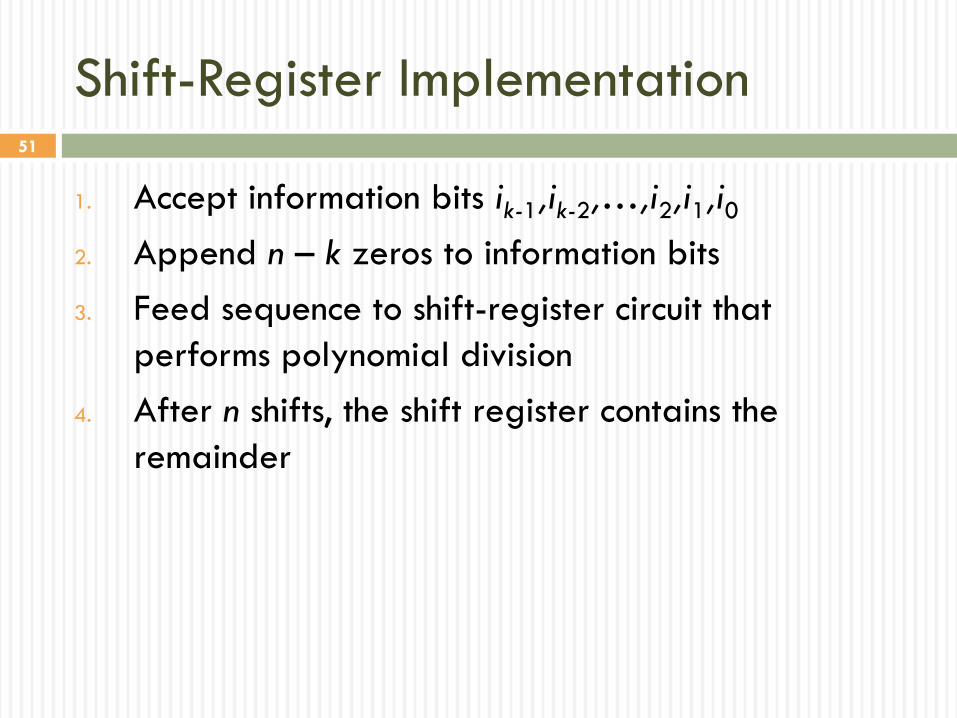
Shift-Register Implementation

1. Accept information bits ik-1,ik-2,…,i2,i1,i0

2. Append n – k zeros to information bits

3. Feed sequence to shift-register circuit that

performs polynomial division

4. After n shifts, the shift register contains the

remainder

52

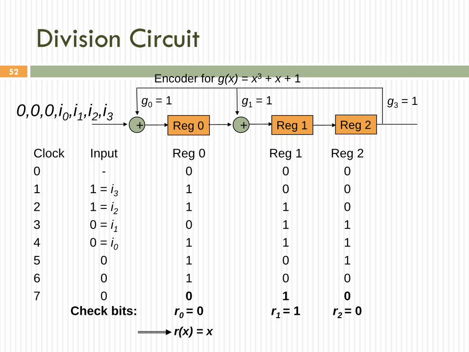
Clock Input Reg 0 Reg 1 Reg 2

0 - 0 0 0

1 1 = i3 1 0 0

2 1 = i2 1 1 0

3 0 = i1 0 1 1

4 0 = i0 1 1 1

5 0 1 0 1

6 0 1 0 0

7 0 0 1 0

Check bits: r0 = 0 r1 = 1 r2 = 0

r(x) = x

Division Circuit

Reg 0 ++

Encoder for g(x) = x3 + x + 1

Reg 1 Reg 20,0,0,i0,i1,i2,i3

g0 = 1 g1 = 1 g3 = 1

53

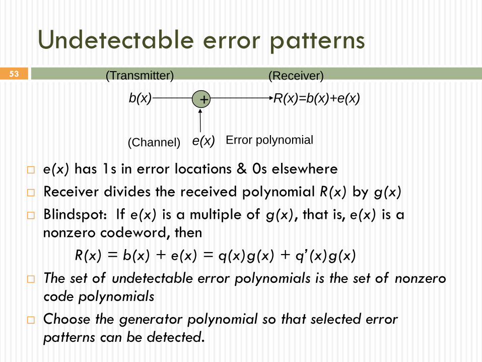
Undetectable error patterns

e(x) has 1s in error locations & 0s elsewhere

Receiver divides the received polynomial R(x) by g(x)

Blindspot: If e(x) is a multiple of g(x), that is, e(x) is a nonzero codeword, then

R(x) = b(x) + e(x) = q(x)g(x) + q’(x)g(x)

The set of undetectable error polynomials is the set of nonzero code polynomials

Choose the generator polynomial so that selected error patterns can be detected.

b(x)

e(x)

R(x)=b(x)+e(x)+

(Receiver)(Transmitter)

Error polynomial(Channel)

54

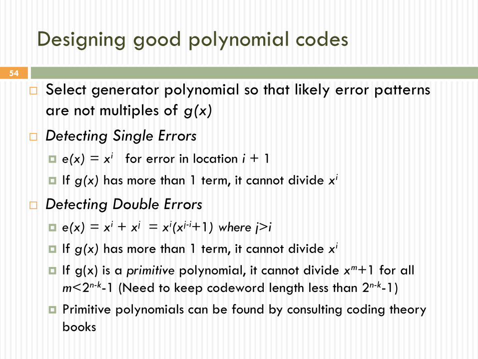
Designing good polynomial codes

Select generator polynomial so that likely error patterns

are not multiples of g(x)

Detecting Single Errors

e(x) = xi for error in location i + 1

If g(x) has more than 1 term, it cannot divide xi

Detecting Double Errors

e(x) = xi + xj = xi(xj-i+1) where j>i

If g(x) has more than 1 term, it cannot divide xi

If g(x) is a primitive polynomial, it cannot divide xm+1 for all

m<2n-k-1 (Need to keep codeword length less than 2n-k-1)

Primitive polynomials can be found by consulting coding theory

books

55

Designing good polynomial codes

Detecting Odd Numbers of Errors

Suppose all codeword polynomials have an even # of

1s, then all odd numbers of errors can be detected

As well, b(x) evaluated at x = 1 is zero because b(x)

has an even number of 1s

This implies x + 1 must be a factor of all b(x)

Pick g(x) = (x + 1) p(x) where p(x) is primitive

56

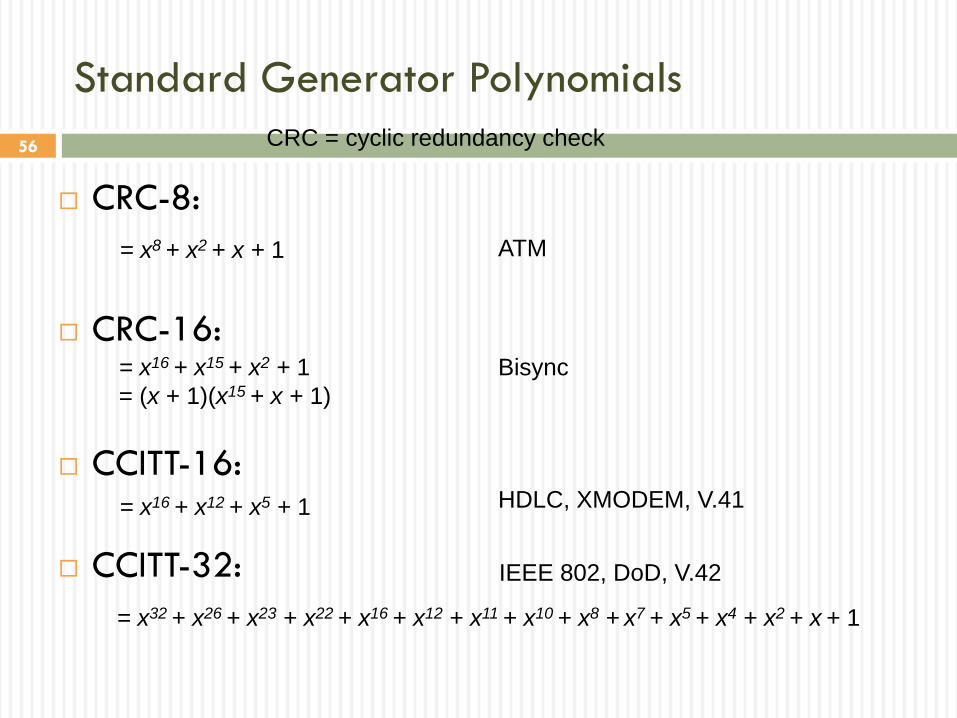
Standard Generator Polynomials

CRC-8:

CRC-16:

CCITT-16:

CCITT-32:

CRC = cyclic redundancy check

HDLC, XMODEM, V.41

IEEE 802, DoD, V.42

Bisync

ATM= x8 + x2 + x + 1

= x16 + x15 + x2 + 1

= (x + 1)(x15 + x + 1)

= x16 + x12 + x5 + 1

= x32 + x26 + x23 + x22 + x16 + x12 + x11 + x10 + x8 + x7 + x5 + x4 + x2 + x + 1

57

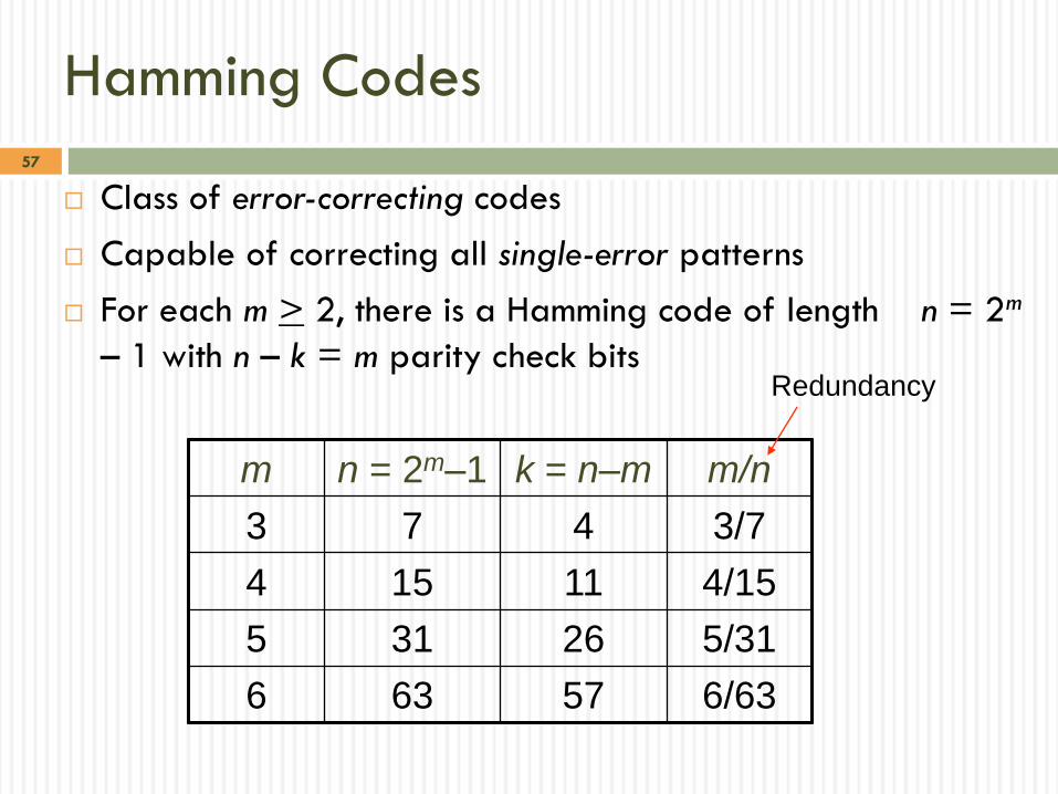
Hamming Codes

Class of error-correcting codes

Capable of correcting all single-error patterns

For each m > 2, there is a Hamming code of length n = 2m

– 1 with n – k = m parity check bits

m n = 2m–1 k = n–m m/n

3 7 4 3/7

4 15 11 4/15

5 31 26 5/31

6 63 57 6/63

Redundancy

58

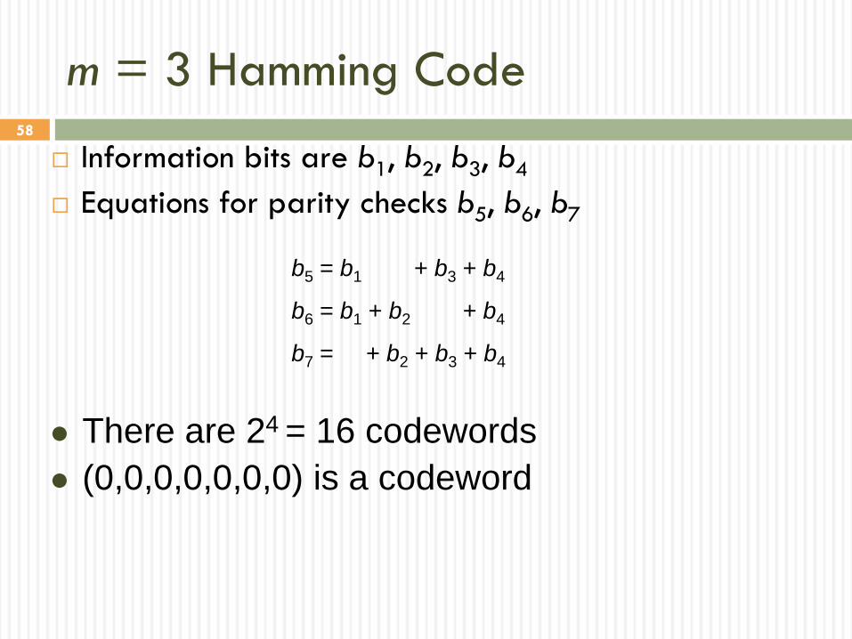
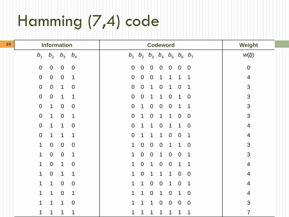
m = 3 Hamming Code

Information bits are b1, b2, b3, b4

Equations for parity checks b5, b6, b7

There are 24 = 16 codewords

(0,0,0,0,0,0,0) is a codeword

b5 = b1 + b3 + b4

b6 = b1 + b2 + b4

b7 = + b2 + b3 + b4

59

Hamming (7,4) code

Information Codeword Weight

b1 b2 b3 b4 b1 b2 b3 b4 b5 b6 b7 w(b)

0 0 0 0 0 0 0 0 0 0 0 0

0 0 0 1 0 0 0 1 1 1 1 4

0 0 1 0 0 0 1 0 1 0 1 3

0 0 1 1 0 0 1 1 0 1 0 3

0 1 0 0 0 1 0 0 0 1 1 3

0 1 0 1 0 1 0 1 1 0 0 3

0 1 1 0 0 1 1 0 1 1 0 4

0 1 1 1 0 1 1 1 0 0 1 4

1 0 0 0 1 0 0 0 1 1 0 3

1 0 0 1 1 0 0 1 0 0 1 3

1 0 1 0 1 0 1 0 0 1 1 4

1 0 1 1 1 0 1 1 1 0 0 4

1 1 0 0 1 1 0 0 1 0 1 4

1 1 0 1 1 1 0 1 0 1 0 4

1 1 1 0 1 1 1 0 0 0 0 3

1 1 1 1 1 1 1 1 1 1 1 7

60

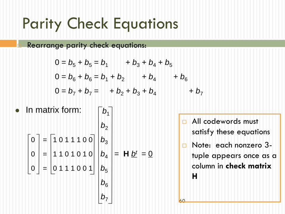
Parity Check Equations Rearrange parity check equations:

All codewords must

satisfy these equations

Note: each nonzero 3-

tuple appears once as a

column in check matrix

H

In matrix form:

0 = b5 + b5 = b1 + b3 + b4 + b5

0 = b6 + b6 = b1 + b2 + b4 + b6

0 = b7 + b7 = + b2 + b3 + b4 + b7

b1

b2

0 = 1 0 1 1 1 0 0 b3

0 = 1 1 0 1 0 1 0 b4 = H bt = 0

0 = 0 1 1 1 0 0 1 b5

b6

b7

61

0

0

1

0

0

0

0

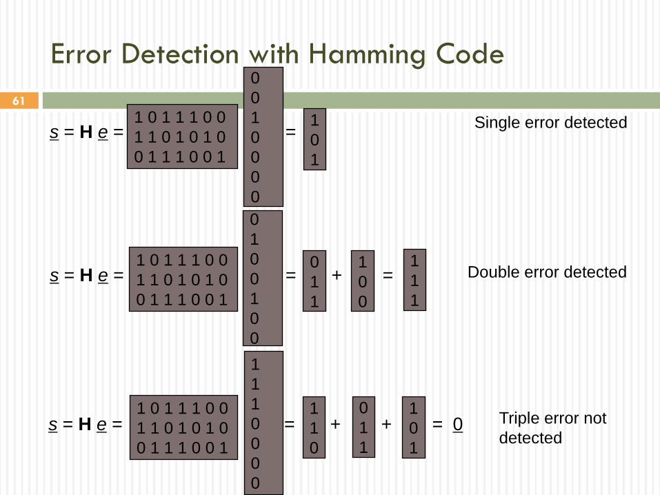
s = H e = =1

0

1

Single error detected

0

1

0

0

1

0

0

s = H e = = + =0

1

1

Double error detected1

0

0

1 0 1 1 1 0 0

1 1 0 1 0 1 0

0 1 1 1 0 0 1

1

1

1

0

0

0

0

s = H e = = + + = 01

1

0

Triple error not

detected

0

1

1

1

0

1

1 0 1 1 1 0 0

1 1 0 1 0 1 0

0 1 1 1 0 0 1

1 0 1 1 1 0 0

1 1 0 1 0 1 0

0 1 1 1 0 0 1

1

1

1

Error Detection with Hamming Code

62

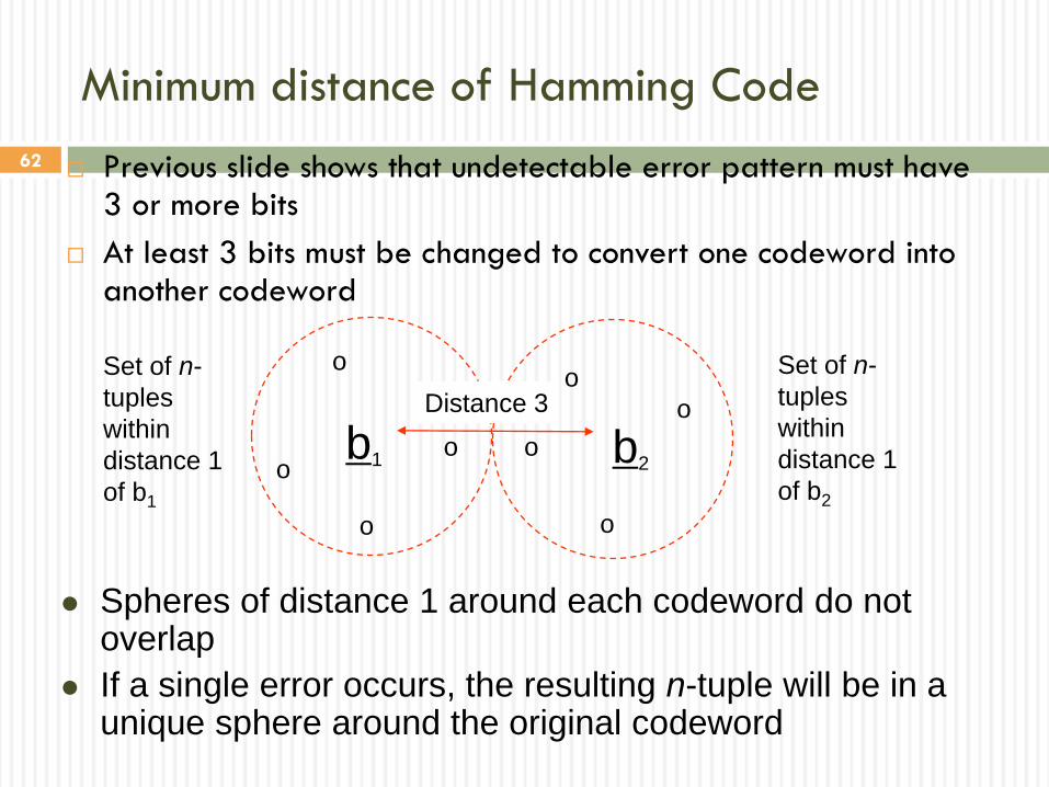
Minimum distance of Hamming Code

Previous slide shows that undetectable error pattern must have 3 or more bits

At least 3 bits must be changed to convert one codeword into another codeword

b1 b2o o

o

o

oo

o

o

Set of n-

tuples

within

distance 1

of b1

Set of n-

tuples

within

distance 1

of b2

Spheres of distance 1 around each codeword do not overlap

If a single error occurs, the resulting n-tuple will be in a unique sphere around the original codeword

Distance 3

63

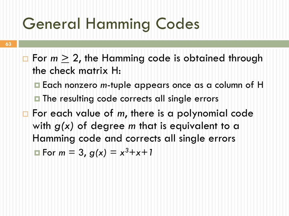
General Hamming Codes

For m > 2, the Hamming code is obtained through the check matrix H:

Each nonzero m-tuple appears once as a column of H

The resulting code corrects all single errors

For each value of m, there is a polynomial code with g(x) of degree m that is equivalent to a Hamming code and corrects all single errors

For m = 3, g(x) = x3+x+1

64

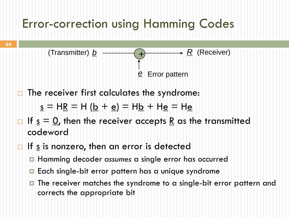
Error-correction using Hamming Codes

The receiver first calculates the syndrome:

s = HR = H (b + e) = Hb + He = He

If s = 0, then the receiver accepts R as the transmitted codeword

If s is nonzero, then an error is detected

Hamming decoder assumes a single error has occurred

Each single-bit error pattern has a unique syndrome

The receiver matches the syndrome to a single-bit error pattern and corrects the appropriate bit

b

e

R+ (Receiver)(Transmitter)

Error pattern

65

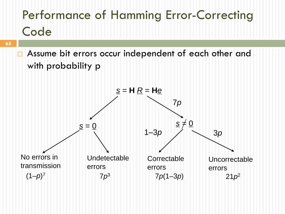
Performance of Hamming Error-Correcting

Code

Assume bit errors occur independent of each other and

with probability p

s = H R = He

s = 0 s = 0

No errors in

transmission Undetectable

errorsCorrectable

errorsUncorrectable

errors(1–p)7 7p3

1–3p 3p

7p

7p(1–3p) 21p2

66

DIGITAL TRANSMISSION

FUNDAMENTALS

RS-232 Asynchronous Data Transmission

Lecture 9

Fall 2009

67

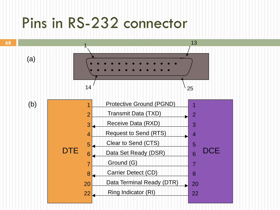
Recommended Standard (RS) 232

Serial line interface between computer and modem

or similar device

Data Terminal Equipment (DTE): computer

Data Communications Equipment (DCE): modem

Mechanical and Electrical specification

68

DTE DCE

Protective Ground (PGND)

Transmit Data (TXD)

Receive Data (RXD)

Request to Send (RTS)

Clear to Send (CTS)

Data Set Ready (DSR)

Ground (G)

Carrier Detect (CD)

Data Terminal Ready (DTR)

Ring Indicator (RI)

1

2

3

4

5

6

7

8

20

22

1

2

3

4

5

6

7

8

20

22

(b)

13

(a)

1

2514

Pins in RS-232 connector

69

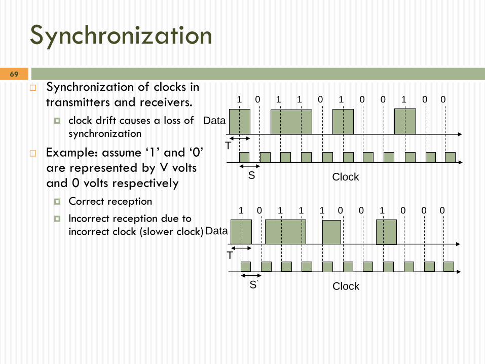
Synchronization

Synchronization of clocks in transmitters and receivers.

clock drift causes a loss of synchronization

Example: assume „1‟ and „0‟ are represented by V volts and 0 volts respectively

Correct reception

Incorrect reception due to incorrect clock (slower clock)

Clock

Data

S

T

1 0 1 1 0 1 0 0 1 0 0

Clock

Data

S’

T

1 0 1 1 1 0 0 1 0 0 0

70

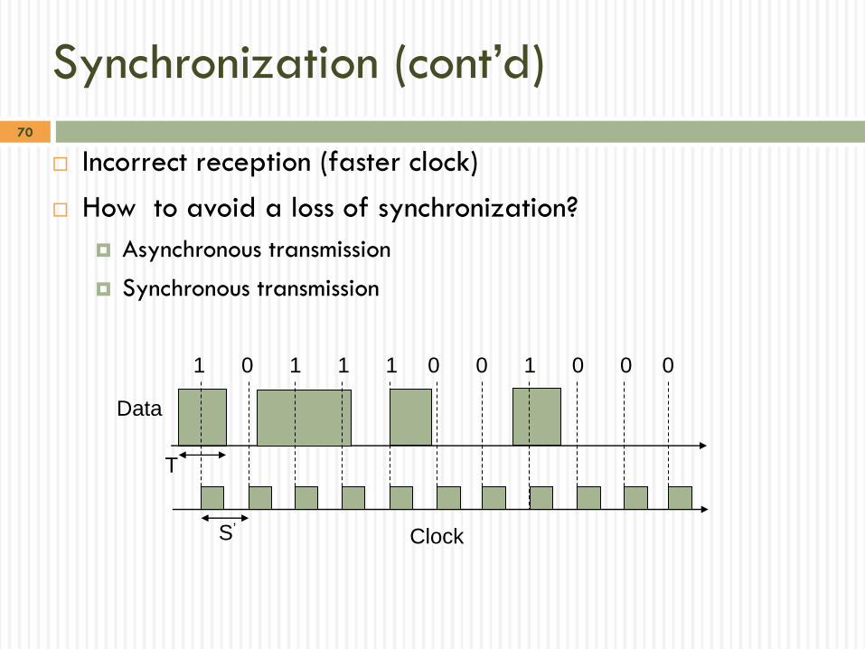
Synchronization (cont‟d)

Incorrect reception (faster clock)

How to avoid a loss of synchronization?

Asynchronous transmission

Synchronous transmission

Clock

Data

S’

T

1 0 1 1 1 0 0 1 0 0 0

71

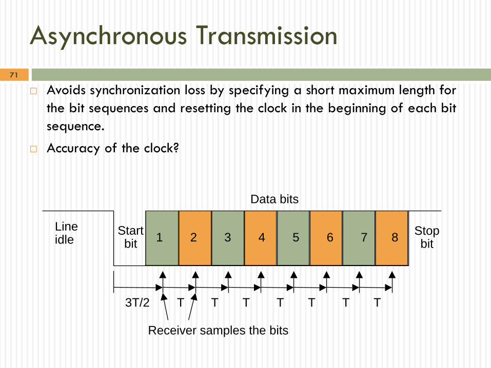
Asynchronous Transmission

Avoids synchronization loss by specifying a short maximum length for

the bit sequences and resetting the clock in the beginning of each bit

sequence.

Accuracy of the clock?

Startbit

Stopbit

1 2 3 4 5 6 7 8

Data bits

Lineidle

3T/2 T T T T T T T

Receiver samples the bits

72

Synchronous Transmission

Voltage

1 0 0 0 1 1 0 1 0

time

Sequence contains data + clock information (line coding)

i.e. Manchester encoding, self-synchronizing codes, is used.

R transition for R bits per second transmission

R transition contains a sine wave with R Hz.

R Hz sine wave is used to synch receiver clock to the transmitter‟s clock using PLL (phase-lock loop)