7–The Nonlinear Wave Equationand the

Interaction of Waves

MATH 22C

1. Introduction

Just as the nonlinear advection equation looks the sameas the linear advection equation ut + cux = 0 except thatthe speed of sound c depends on the solution u, so alsothe nonlinear wave equation is the linear wave equationutt − c2uxx = 0 under the assumption that the speed ofsound c depends on the solution u as well. Now for theadvection equation, the solution, being a single wave

u(x, t) = f(x− ct)moving to the right, is constant along curves x−ct = const.These so called characteristic curves are the sound wavesmoving at the speed of sound c in the (x, t)-plane. Thussound wave propagation occurs along curves (x(t), t) satisy-ing

x = c,

as they should. When c depends on u, for example c = uis the Burger’s equation, then solutions u(x, t) still remainconstant along the characteristics

x = c(u),

but since the speeds depend on the solution, characteristicscan intersect and create shock waves. But the connectionbetween the sound waves in the linear advection equationut + cux = 0 and the nonlinear advection equations, (sayBurgers equation ut + uux = 0) is clear: The nonlinearwave moves the constant value u along lines of speed u inthe (x, t) plane, thereby creating an approximate wave of

1

2

speed c when u takes values near the the constant value c.

Now the wave equation is a more realistic model for soundwave propagation than the advection equation because itis obtained by linearizing the compressible Euler equationsabout a constant state. The advection equations ut+cux =0 and ut − cux = 0 admit the right and left going wavesseparately, but the wave equation admits the superpositionof both waves, and we have shown that all solutions of thewave equation decompose into a left and right going waveof form

u(x, t) = f(x+ ct) + g(x− ct).

But a solution of the wave equation, being in general asuperposition of both left and right going waves, is onlyconstant along the characteristic curves dx/dt = ±c whenthe wave is a pure left (g = 0) or pure right (f = 0) go-ing wave. In general, the superposition mixes up the rightand left moving waves and the solution will not be constantalong the characteristics dx/dt = ±c. To understand thecharacteristics in a way that generalizes to nonlinear waveequations in which the speed c depends on the solution,we need a more general framework that breaks the solutiondown into identifiable components. The goal is to see thatthe nonlinear wave equation also admits nonlinear wavesthat propagate to the right and to the left, but being non-linear, superposition fails, and a general solution does notexactly decompose into a sum of left and right going wavesas do solutions of the linear (constant c) wave equation. Tounderstand what we might call the nonlinear superpositionof left and right going waves created by the nonlinear waveequation, we develop a more general method that treatsthe wave equation as a first order system, and is based on

3

finding Riemann invariants: functions r and s of the un-knowns that are constant along sound waves, that is, con-stant along the characteristic curves in the (x, t)-plane. Bythis we can explain the propagation of left and right goingnonlinear waves along the characteristics ds/dt = ±c, whenc depends on the solution.

To write the wave equation as a first order system, assume

wtt − c2wxx = 0,

view w as a potential, and set wt = u, wx = v to get the2× 2 first order system

vt − ux = 0, (1)

ut − c2vx = 0, (2)

valid whether c is constant, or c depends on the unknownsu, v. The first equation (1) expresses that mixed partialswxt = wtx are equal, and the second equation (2) expressesthe wave equation. Equations (1), (2) take the matrix form(

vu

)t

+

(0 −1−c2 0

)(vu

)x

= 0,

a general first order system of the form

Ut + AUx = 0, (3)

where U = (v, u) and A is a 2 × 2 matrix. The main goalof this section is to explain how the eigenpairs (λ,R) of Adecouple the nonlinear wave equation into its left and rightmoving component waves.

All of this is worth the trouble because we show that,when rewritten as an equivalent system in a coordinateframe moving with the fluid, the compressible Euler equa-tions take the exact form of the nonlinear wave equationutt − c2uxx = 0, where c depends on the solution. (This

4

is the so called Lagrangian formulation of the compress-ible Euler equations.) That is, since the sound speed is thespeed of sound waves relative to the fixed fluid, we knowwe can only get the linear wave equation (with wave prop-agation at speed c in both directions) by linearizing theequation in a coordinate frame fixed with the medium ofpropagation. (We assume no relativity to make the speedsthe same in every frame!) In a general solution of the non-linear equations, the fluid velocity u varies from point topoint, so we can’t get a global frame fixed with the mediumof propagation. Thus we do the next best thing. To turnthe Euler equations into the nonlinear wave equation, wetransform x and t so that at each point in the solution weare moving with the fluid. The transformation thus de-pends on the solution. The resulting equations obtainedby transforming the original compressible Euler equations

ρt + (ρu)x = 0, (4)

(ρu)t + (ρu2 + p)x = 0, (5)

by a solution dependent transformation that moves withthe medium at every point, results in the equivalent systemof two equations

vt − ux = 0, (6)

ut + p(v)x = 0, (7)

in the two unknowns

v = 1/ρ = specific volume, (8)

u = velocity. (9)

The original equations (4), (5) are called the Eulerian for-mulation of the equations and the equivalent transformedequations (6), (7) are called the Lagrangian formulation ofthe equations. The Lagrangian measure of distance x ap-pearing in (6), (7), constructed to measure the distance

5

between fluid particles as constant, is different from theEulerian x appearing in (4), (5), as will be clarified in thethe derivation of (6), (7) below. In the Lagrangian version,the equation of state expresses the pressure p = p(v) as afunction of specific volume v = 1/ρ, and since this is theonly nonlinear function in the equations, these equationsare called the p-system, (so named by Joel Smoller). Thep-system provides the simplest realistic quantitative modelfor shock wave propagation down a one dimensional shocktube. Comparing (6), (7) with (1), (2), we see that the thep-system agrees with the nonlinear wave equation writtenas a first order system if we make the identification

c =√−p′(v).

Recall that for the linearized Euler equations

ρtt − c2ρxx = 0,

the sound speed was

c =

√dp

dρ=

√dp

dv

dv

dρ=

√−p′(v)

ρ,

the extra factor of ρ in the denominator accounting for thedifference between the Eulerian and Lagrangian version ofthe equations.

Finally, we can reverse the steps and recover the nonlinearwave equation from the p-system (6),(7) as follows. By thefirst equation (6) we have

Curl(x,t)(v, u) = (ux − vt)k = 0,

so from vector calculus we know that this is the conditionrequired for the vector field (v(x, t), u(x, t)) to be the gra-dient of some function w(x, t); i.e., there exists a potentialfunction w such that

∇(x,t)w = (wx, wt) = (v, u).

6

Thus v = wx and u = wt. Equation (7) thus gives us theequation for the potential w,

wtt + p′(v)wxx = 0. (10)

Note that p′(v) < 0 because pressure increases with density,and decreases with inverse density v = 1/ρ. Thus p′(v) =−|p′(v)|, and (10) really is the wave equation

wtt − c2wxx = 0 (11)

with nonlinear sound speed c = c(v) =√−p′(ρ) > 0. Thus

again, the speed of sound for the p-system, written as anonlinear wave equation, is c =

√−p′(v), and the p-system

written in terms of the potential is the nonlinear wave equa-tion wtt − c2wxx = 0.

2. The p-system

We now show that the compressible Euler equations (4),(5), which describe the nonlinear wave motion of the den-sity and velocity of a gas propagating down a one dimen-sional shock tube, really can be written as the nonlinearwave equation (6), (7). That is, recall that we obtainedthe wave equation ρtt − c2ρxx = 0 by linearizing the com-pressible Euler equation in a frame fixed with respect thefluid; i.e., about a constant state ρ = ρ0, u = u0 = 0. Inthis frame, the velocity u0 is zero, so the gas is not moving.Only in this frame can we get the wave equation becausethe wave equation has two equal sound speeds ±c movingin both directions, something we would not see if the fluidwere say moving to the right with velocity u0 > 0. Thesame situation occurs for the fully nonlinear Euler equa-tions (4), (5). That is, since the nonlinear wave equationalso has nonlinear sound speeds ±c(v) depending on thevalue v in the solution, sound waves move in both direc-tions at the same speed at each point of a solution, so wecan only get the nonlinear wave equation in a coordinate

7

system fixed with respect to the fluid at every point of thefluid. To achieve this, for each given solution ρ(x, t), u(x, t),we make a change from x-coordinate to ξ-coordinate so that

x = x(ξ, t),

moves with the fluid.

Before constructing the change of variable x = x(ξ, t) thataccomplishes this, we first note that (5) can be written inthe convenient form

ut + uux + px/ρ = 0. (12)

To see this, use the product rule on (5) to obtain

(ρu)t + (ρu2 + p)x = ρtu+ ρut + (ρu)xu+ ρuux + px

= u(ρt + (ρu)x) + ρ(ut + uux + px/ρ),

so since

ut + (ρu)x = 0

by (6), we obtain (12) by dividing by ρ. Thus we can takethe compressible Euler equations to be the system

ρt + (ρu)x = 0, (13)

ut + uux + px/ρ = 0. (14)

One payoff for writing the second equation in this form isto see that when the pressure is zero, then px = 0 as well,and the second equation reduces exactly to the scalar Burg-ers equation. Thus solution to Burgers is a real problemfor fluids.

Our purpose now is to define a change of coordinates

x = x(ξ, t)

such that at each fixed ξ,

x = x(ξ, t)

8

gives x as a function of t moving with the fluid particle atevery point. We then show that when we write (6), (7) interms of (ξ, t) we obtain the p-system

vt − uξ = 0, (15)

ut + p(v)ξ = 0. (16)

which is exactly (6), (7) upon renaming ξ as x.

To this end, assume the velocity field u(x, t) for a solu-tion of the compressible Euler equations (13), (14) is given.That is, u(x, t) is the velocity of the so-called fluid particleat position x at time t, the velocity of a speck of dust mov-ing with the fluid. Keep in mind that u(x, t) is differentfrom the sound speed c. I.e., we’ve seen that sound wavepropagates at a speed ±c relative to the fluid particles. Forexample, the speck of dust starting at x = 0 at time t = 0moves along a curve x0(t) at speed x0(t) = u(x0(t), t), sox0(t) solves the initial value problem

x = u(x(t), t),

x(0) = 0.

Similarly, the dust particle starting at x = a at time t = 0moves along a curve xa(t) at speed x0(t) = u(x(t), t), soxa(t) solves the initial value problem

x = u(x(t), t),

x(0) = a.

Thus we can define the general solution xa(t) = x(a, t) asthe position at time t of particle that started at positionx = a at time t = 0. In particular, the particles are movingat speed u, so we know that for fixed a (that fixes theparticle),

xa(t) = u,

9

where u is the speed at position x = xa(t), time t. In termsof partial derivatives, this is expressed by

∂x

∂t(a, t) = u(x(a, t), t).

Now for the clever part. We define ξ to be a function ofthe initial positions a by

ξ =

∫ a

0

ρ(x, 0)dx. (17)

That is, ξ is the function of a equal to the amount of massbetween x = 0 and x = a at time t = 0. If you fix a, youfix ξ as well, and vice versa. Fixing a is the same as fixingξ. So we can write the particle path as xξ(t) = x(ξ, t), andby the same argument

xξ(t) = u,

where u is the speed at position x = xξ(t), time t. In termsof partial derivatives this is expressed by

∂x

∂t(ξ, t) = u(x(ξ, t), t).

In particular, for any function of f(x, t), we can write

f(x(ξ, t), t)

to express it as a function (ξ, t), and so by differentiatingf with respect to t holding ξ fixed we obtain the rate atwhich f changes along the particle path. That is, by thechain rule

∂

∂tf(x(ξ, t), t) =

∂f

∂x

∂x

∂t+∂f

∂t= ft + fxu.

This is called the material derivative of f because it is therate at which f changes as measured in a frame moving withthe material. Note that all we need is that ξ is a function of

10

a to compute the time derivative of f holding ξ fixed (thematerial derivative), but to compute

∂

∂ξf(x(ξ, t), t) =

∂f

∂x

∂x

∂ξ,

we need the formula for ∂∂ξx(ξ, t).

To complete the task of deriving the p-system, we now showthat, when written in terms of the transformed variable ξ,the compressible Euler equations (13), (14) reduce to thep-system, that is, they take the form of the nonlinear waveequation. For this we need to compute ∂

∂ξx(ξ, t) which wedo by use of the following fact which states that the totalmass between two particle paths is constant in time:

ξ =

∫ a

0

ρ(x, 0)dx =

∫ xξ(t)

x0(t)

ρ(x, t)dx ≡Mξ(t), (18)

where the ≡ defines Mξ(t). The first equality in (18) isintuitively clear because Mξ(t) is the total mass betweenthe particle path x0(t) and xξ(t) at time t, and mass is con-served, which implies Mξ is constant with Mξ(t) = Mξ(0) =ξ. Thus to verify the first equality in (18) it suffices to provethat Mξ(t) = 0. In fact, (18) follows directly from (13).Before proving this, we point out that the main purpose of(18) is that from this we can calculate ∂x/∂ξ by taking thepartial derivative of (18) with respect to ξ on both sides ofthe first equality sign to get

1 =∂

∂ξ

∫ xξ(t)

x0(t)

ρ(x, t)dx = ρ∂x

∂ξ, (19)

which we can solve for ∂x/∂ξ to get

∂x

∂ξ=

1

ρ,

11

and its reciprocal

∂ξ

∂x= ρ,

To verify the first equality in (18) we need only to showthat M ′(t) = 0, (because then Mξ(t) = Mξ(0) = ξ). Butby the chain rule for integrals,

M ′ξ(t) =

d

dt

∫ xξ(t)

x0(t)

ρ(x, t)dx =d

dt

∫ x(ξ,t)

x(0,t)

ρ(x, t)dx

= ρ(x(ξ, t), t)x′ξ(t)− ρ(x(0, t)x′0(t) +

∫ x(ξ,t)

x(0,t)

ρt(x, t)dx.

But the speed of the particle paths is u so

x′ξ(t) = u(x(ξ, t), t), (20)

x′0(t) = u(x(ξ, 0), 0), (21)

and using (13) in the form ρt = −(ρu)x gives∫ x(ξ,t)

x(0,t)

ρt(x, t)dx = −∫ x(ξ,t)

x(0,t)

(ρu)x(x, t)dx

= −{(ρu)(x(ξ, t), t)− (ρu)(x(ξ, 0), 0)} .Substituting (21)-(22) into the last line of (20) gives

M ′(t) = {(ρu)(x(ξ, t), t)− (ρu)(x(0, t), t)}−{(ρu)(x(ξ, t), t)− (ρu)(x(0, t), t)} = 0,

verifying (18) as claimed.

We now have everything we need to show that when ξ istaken in place of x, the compressible Euler equations con-vert to the p-system, a first order version of the nonlinearwave equation. All we need is

x = x(ξ, t),

12

with the partial derivative formula

ξx ≡∂ξ

∂x(x, t) = ρ,

and material derivative formulas

ρt + uρx =∂

∂tρ(ξ, t), (22)

ut + uux =∂

∂tu(ξ, t). (23)

So here it is:

To transform equation (13) write

0 = ρt + (ρu)x = (ρt + ρxu) + ρux

=∂

∂tρ(ξ, t) + ρuξ(ξ, t)ξx

= ρt(ξ, t) + ρ2uξ(ξ, t),

which we can rewrite as1

ρ2ρt + uξ = 0,

which gives the desired first equation (6) of the p-system

vt − uξ = 0,

since v = 1/ρ makes

vt =

(1

ρ

)t

= −ρtρ2.

To transform equation (5) write

0 = ut+uux+px/ρ =∂

∂tu(ξ, t)+

∂p

∂ξξx

1

ρ= ut(ξ, t)+pξ(ξ, t),

which isut + p(v)ξ = 0,

in agreement with (7) upon renaming ξ as x.

13

Conclude: The compressible Euler equations when writ-ten in terms of the Lagrangian variable ξ transform intothe nonlinear wave equation (6), (7).

3. Riemann Invariants and the Interaction ofNonlinear Waves

We have written the wave equation wtt − c2wxx = 0 as afirst order system

vt − uξ = 0, (24)

ut − c2vx = 0, (25)

with u = wt and v = wx, and we found that the compress-ible Euler equations in Lagrangian coordinate ξ (which wenow write as x) reduce to the p-system

vt − uξ = 0,

ut + p(v)ξ = 0,

where u is the velocity and v = 1/ρ is called the specificvolume. Writing

p(v)x = p′(v)vx = −c2vx,with

c =√−p′(v)

we see that the p-system takes the form of the wave equa-tion (24), (25), but it’s now the nonlinear wave equationbecause c depends on the unknown v. Before describingsolutions of the linear and nonlinear wave equations, weconsider two specific equations of state p = p(v) of inter-est.

• First, recall the ideal gas law relating the pressure p of agas of N molecules in a container of volume V

pV = NRT,

14

where T is the temperature (in degrees Kelvin so T > 0)and R is the universal gas constant. In this case, if we di-vide by the total mass M of all N molecules in the containerwe get

pV

M=N

MRT = KT,

where K is constant, and V/M is then specific volume v.Assuming the temperature is constant,

KT = σ2 > 0

results in the isothermal equation of state

p(v) =σ2

v.

In this case

p′(v) = −σ2

v2, (26)

and the sound speed c(v) in (24), (25) is

c(v) =σ

v.

Of course this is the speed of sound dx/dt as measured inthe Lagrangian frame moving with the fluid. In the Euler-ian frame (physical space) the speed of sound

√p′(ρ) = σ

is constant in the isothermal case. It turns out that fordifferent reasons, the equation of state p proportional to ρis correct in the relativistic setting for pure radiation, andis taken as correct during the radiation phase of the BigBang, after inflation, up to several hundred thousand yearsafter the Big Bang, c.f. [?].

A second important case is the so called isentropic or γ lawgas in which the equation of state is given by

p(v) =σ2

vγ, (27)

15

where γ > 1. In this case the sound speed in (24), (25)should be taken to be

c(v) =√−p′(v) =

σ√γ

vγ+12

.

More generally, motivated by the isothermal and isentropicequations of state, we define the so-called p-system as thesystem of equations

vt − ux = 0

ut + p(v)x = 0

where p(v) is a general function satisfying the conditionsp(v) > 0, p′(v) < 0, p′′(v) > 0. These are the salientfeatures of p required for the theory to be essentially thesame, and include, the physical cases (??) and (??).

• Our purpose now is to identify the left and right goingwaves associated with the nonlinear wave equation (24),(25), and to describe the nonlinear interaction of such waves.Recall that we have identified the left and right going wavesf(x+ct) and g(x−ct) of the wave equation using the princi-ple of superposition—that sums and multiples of solutionsremain solutions. This method required that the soundspeed c be constant so that the wave equation would behomogeneous and linear, the conditions under which theprinciple of superposition is valid. For the nonlinear waveequation, this method is doomed to failure because c = c(v)depends on the unknown solution, the equations are non-linear, and the principle of superposition fails for nonlinearequations. We first construct the left and right going wavesof the linear wave equation by constructing the Riemanninvariants for its equivalent 2×2 system (24), (25). We willthen extend this method to uncover the left and right goingelementary waves of the nonlinear wave equation, and useit to describe the nonlinear interaction of elementary waves.

16

By this route we discover a new sort of nonlinear superpo-sition principle that describes the interaction of elementarynonlinear right and left going waves.

• To start, consider the linear wave equation

vt − uξ = 0, (28)

ut − c2vx = 0, (29)

under the assumption that c = const. We first define thecharacteristic curves, that is, the trajectories (x(t), t) of theleft and right moving sound waves.

Definition 1. The 1-characteristic curves, or back char-acteristics, are the curves (x(t), t) moving in direction ofnegative x at characteristic (sound) speed

dx

dt= −c. (30)

The 2-characteristic curves, or forward characteristics, arethe curves (x(t), t) moving in direction of positive x at char-acteristic (sound) speed

dx

dt= c. (31)

Now we have seen that a solution w is constant along 1-and 2- characteristics for pure left and right moving wavesf(x + ct) and g(x − ct), but not for the superposition oftwo such waves. The following theorem identifies individ-ual functions r(u, v) and s(u, v) called Reimann invariants,such that r is constant along 1-characteristics and s is con-stant along 2-characteristics for any solution (v, u) of (26),(27):

Theorem 2. The function

r(u, v) = u+ cv (32)

17

is constant along 1-characteristics curves, and

s(u, v) = u− cv (33)

is constant along 2-characteristic curves.

Proof: For (30), use the notation

r(x, t) ≡ r(u(x, t), v(x, t)) = u(x, t) + cv(x, t)

and differentiate r(x(t), t) along a 1-characteristic (x(t), t)using dx/dt = −c:

d

dtr(x(t), t)) = rx

dx

dt+ rt = −crx + rt

= −c(u+ cv)x + (u+ cv)t

= c(vt − ux) + (ut − c2ux) = 0,

the last two parentheses being zero by the equations (26),(27) that (v, u) are assumed to satisfy. By similar reason-ing, s is constant along 2-characteristics. �

The Riemann invariants r and s tell us how to uncover theleft and right going waves. Consider first the right going2-waves. To construct them, restrict to solutions in whichr is everywhere constant,

r(x, t) = r0 = constant.

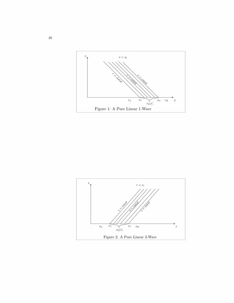
Under this assumption, we can create a localized 2-wavefrom initial data s0(x) localized between x1 ≤ x ≤ x2, (c.f.Figure 2),

s0(x) =

sL, x < x1s0(x), x1 ≤ x ≤ x2,sR, x2 < x.

(34)

We can continue the solution from initial values at t = 0 bytaking s to be constant along the 2-characteristics of speedc emanating from any initial point x at t = 0. In particular,r = r0 = constant is consistent with the equations because

18

all derivatives of the constant state are zero. We need onlyassume the initial data s0(x) is continuous to ensure theprocedure produces a continuous solution moving to theright for all time. Such a simple 2-wave moving to theright is diagrammed in Figure 2.

Consider next the left going 1-waves. To construct them,restrict to solutions in which s is everywhere constant,

s(x, t) = s0 = constant.

Under this assumption, we can create a localized 1-wavefrom initial data r0(x) localized between x3 ≤ x ≤ x4:

r0(x) =

rL, x < x3r0(x), x3 ≤ x ≤ x4,rR, x4 < x.

(35)

Again, we can continue the solution from its initial valuesby taking r to be constant along the 1-characteristics ofspeed x = −c emanating from initial points x at t = 0. Inparticular, r = r0 = constant is consistent with the equa-tions because all derivatives of the constant state are zero.We need only assume the initial data r0(x) is continuous toensure the procedure produces a continuous solution mov-ing to the left for all time. A simple 1-wave moving to theleft is diagrammed in Figure 1.

Using the Riemann invariants, we can understand how theleft and right moving simple waves interact and separate.For this consider the initial data obtained by concatenat-ing the simple wave data (32), (33), as diagrammed in Fig-ure 3. Since r is constant along 1-characteristics and s isconstant along 2-characteristics, the initial waves are sepa-rated because of the background constant state sR on theinitial 1-wave and rL on the initial 2-wave. The waves theninteract in a diamond shaped region where both r and sare changing in time, and finally the waves separate, the

19

outgoing waves of the interaction propagating against thebackground constant states sL and rR of the the oppositeRiemann invariants. (See Figure 3.)

20

x

t

r0(x)rRrL

r=

const

r=

const

r=

const

s = s0

x3 x4

Figure 1: A Pure Linear 1-Wave

Figure 2: A Pure Linear 2-Wave

x

t

s0(x)sL sRx1 x2

r = r0

s=

cons

ts=

cons

ts=

cons

t

21

x

t

r0(x)rRrL

r=

const

s0(x)sL

sR

r=

const

Figure 3: Interaction of Linear Waves

s=

cons

t

s=

cons

t

x

t

r0(x) s0(x)

r=

const

x1 x2,

(x, t)

x=

x 1+

ct x=

x2 −

ct

Figure 4: Formula for Solution when c = Constant.

r(x, t) = u(x, t) + cv(x, t)

s(x, t) = u(x, t) − cv(x, t)

u(x, t) =r(x2, 0) + s(x1, 0)

2

s(x, t) = s(x1, 0)r(x, t) = r(x2, 0)

s=

cons

t

v(x, t) =r(x2, 0) − s(x1, 0)

2c

22

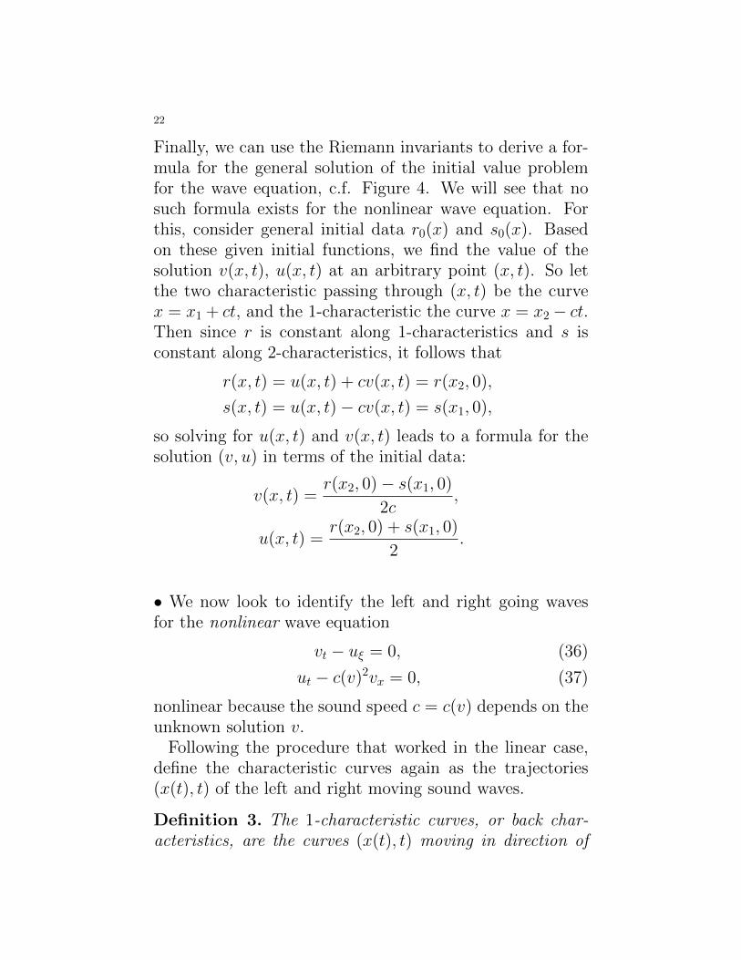
Finally, we can use the Riemann invariants to derive a for-mula for the general solution of the initial value problemfor the wave equation, c.f. Figure 4. We will see that nosuch formula exists for the nonlinear wave equation. Forthis, consider general initial data r0(x) and s0(x). Basedon these given initial functions, we find the value of thesolution v(x, t), u(x, t) at an arbitrary point (x, t). So letthe two characteristic passing through (x, t) be the curvex = x1 + ct, and the 1-characteristic the curve x = x2− ct.Then since r is constant along 1-characteristics and s isconstant along 2-characteristics, it follows that

r(x, t) = u(x, t) + cv(x, t) = r(x2, 0),

s(x, t) = u(x, t)− cv(x, t) = s(x1, 0),

so solving for u(x, t) and v(x, t) leads to a formula for thesolution (v, u) in terms of the initial data:

v(x, t) =r(x2, 0)− s(x1, 0)

2c,

u(x, t) =r(x2, 0) + s(x1, 0)

2.

• We now look to identify the left and right going wavesfor the nonlinear wave equation

vt − uξ = 0, (36)

ut − c(v)2vx = 0, (37)

nonlinear because the sound speed c = c(v) depends on theunknown solution v.

Following the procedure that worked in the linear case,define the characteristic curves again as the trajectories(x(t), t) of the left and right moving sound waves.

Definition 3. The 1-characteristic curves, or back char-acteristics, are the curves (x(t), t) moving in direction of

23

negative x at characteristic (sound) speed

dx

dt= −c(v(x, t)). (38)

The 2-characteristic curves, or forward characteristics, arethe curves (x(t), t) moving in direction of positive x at char-acteristic (sound) speed

dx

dt= c(v(x, t)). (39)

But now because in the nonlinear case the sound speed c(v)is not constant, the ODE’s can be solved only when v(x, t)is known, that is, only after a solution (v, u) of (34), (35)is given. Said differently, in the nonlinear case the char-acteristic curves depend on the solution—as they shouldbecause sound speeds really do depend on the density. Soassume a solution, and hence v(x, t) is given, and the 1-and2-characteristic curves are defined. The following theoremidentifies the Riemann invariants r(u, v) and s(u, v) satisfy-ing the condition that r is constant along 1-characteristicsand s is constant along 2-characteristics for any solution(v, u) of (26), (27).

Theorem 4. Let h(v) be an anti-derivative of c(v),

h′(v) = c(v).

Then for any solution v(x, t), u(x, t) of (38), (39), the func-tion

r(u, v) = u+ h(v) (40)

is constant along 1-characteristics curves, and

s(u, v) = u− h(v) (41)

is constant along 2-characteristic curves.

Proof: For (38), use the notation

r(x, t) ≡ r(u(x, t), v(x, t)) = u(x, t) + h(v(x, t)),

24

and differentiate r(x(t), t) along a 1-characteristic (x(t), t)using dx/dt = −c(v):

d

dtr(x(t), t)) = rx

dx

dt+ rt = −c(v)rx + rt

= −c(v)(u+ h(v))x + (u+ h(v))t

= −c(v)(ux + h′(v)vx) + (ut + h′(v)vt)

= c(v)(vt − ux) + (ut − c(v)2vx) = 0,

where we have used h′(v) = c(v) and that the last twoparentheses are zero by the equations (34), (35). By similarreasoning, s is constant along 2-characteristics. �

The Riemann invariants r and s enable us to unravel theleft and right going waves for the nonlinear wave equation.Consider first the right going 2-waves. To construct them,restrict again to solutions in which r is everywhere con-stant,

r(x, t) = r0 = constant.

Under this assumption, we can again create a localized 2-wave from initial data s0(x) localized between x1 ≤ x ≤ x2:

s0(x) =

sL, x < x1s0(x), x1 ≤ x ≤ x2,sR, x2 < x.

(42)

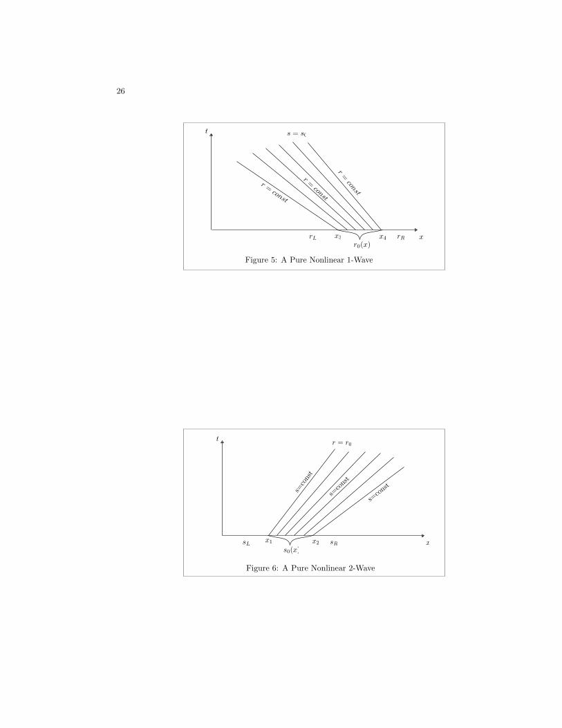
We can continue the solution from initial values at t = 0by taking s to be constant along the 2-characteristics ofspeed c(v) emanating from any initial point x at t = 0. Inparticular, r = r0 = constant is again consistent with theequations because all derivatives of the constant state arestill zero. We need only assume the initial data s0(x) iscontinuous to ensure the procedure produces a continuoussolution moving to the right for all time. A simple nonlinear2-wave moving to the right is diagrammed in Figure 6.

25

However, remarkably, even though the speed x(t) = c(v) ofthe characteristic curves (x(t), t) depends on the solutionv(x, t), along the simple 2-wave, the speed of each individ-ual characteristic is constant, (albeit a different constantfor each characteristic), because both r and s and henceboth u and v are constant along characteristics. That is,r = r0 fixes r, and s is constant along each 2-characteristicby our theorem. The main point is then that the sim-ple 2-wave is propagating against a constant backgroundvalue r0 of the opposite Riemann invariant. As soon as theopposite Riemann invariant r starts changing along the 2-characteristic, the speeds of the 2-characteristic curves willchange due to the nonlinearities, and so the characteristiccurves will no longer be straight lines. This change of wavespeed is indicated in Figure 7.

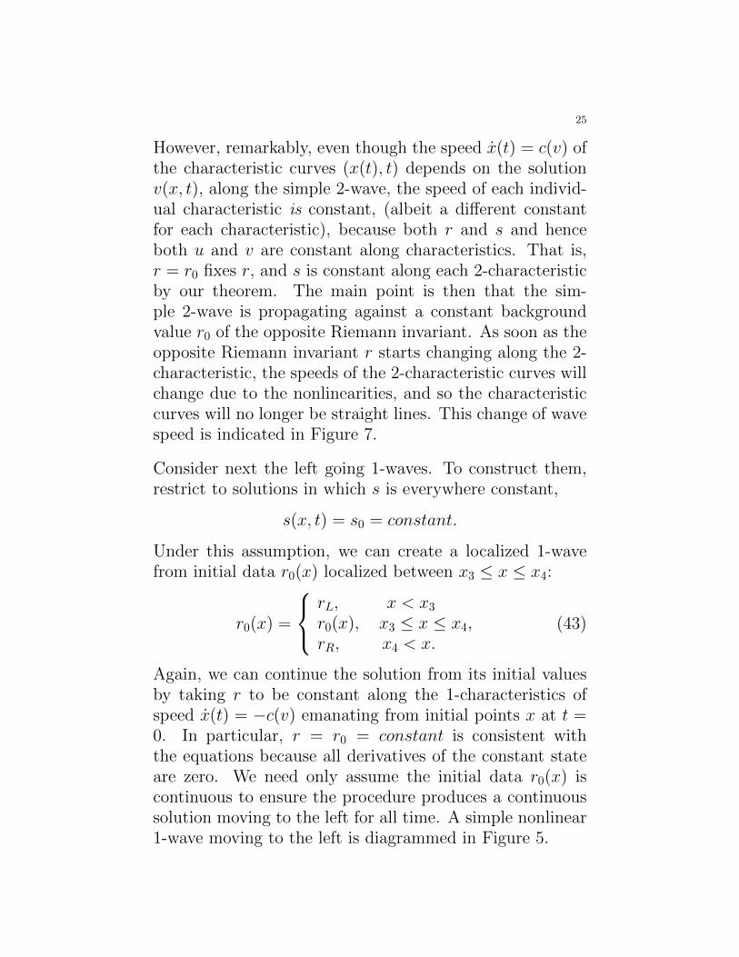
Consider next the left going 1-waves. To construct them,restrict to solutions in which s is everywhere constant,

s(x, t) = s0 = constant.

Under this assumption, we can create a localized 1-wavefrom initial data r0(x) localized between x3 ≤ x ≤ x4:

r0(x) =

rL, x < x3r0(x), x3 ≤ x ≤ x4,rR, x4 < x.

(43)

Again, we can continue the solution from its initial valuesby taking r to be constant along the 1-characteristics ofspeed x(t) = −c(v) emanating from initial points x at t =0. In particular, r = r0 = constant is consistent withthe equations because all derivatives of the constant stateare zero. We need only assume the initial data r0(x) iscontinuous to ensure the procedure produces a continuoussolution moving to the left for all time. A simple nonlinear1-wave moving to the left is diagrammed in Figure 5.

26

x

t

r0(x)rRrL

r=

const

r=

const

r =const

s = s0

x3 x4

Figure 5: A Pure Nonlinear 1-Wave

x

t

s0(x)sL sR

s=co

nst

s=co

nst

s=co

nst

x1 x2

r = r0

Figure 6: A Pure Nonlinear 2-Wave

27

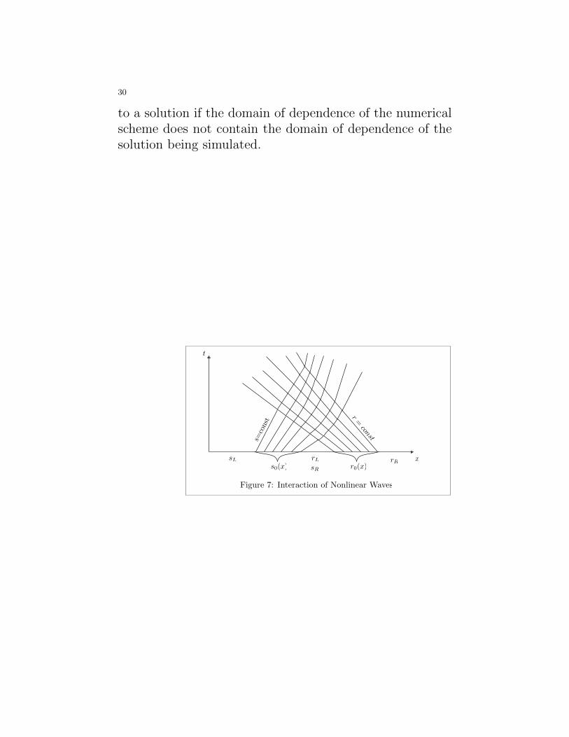
Using the Riemann invariants, we can understand how theleft and right moving nonlinear simple waves interact andseparate. For this consider the initial data obtained by con-catenating the simple wave data (40), (41), as diagrammedin Figure 7. Since r is constant along 1-characteristics ands is constant along 2-characteristics, the initial waves areseparated because of the background constant state sR onthe initial 1-wave and rL on the initial 2-wave. Before inter-action, the both characteristics propagate with a constantspeed and hence are straight lines, because both Riemanninvariants r and s, and hence u and v, and hence c(v), areconstant along each characteristic. The speeds of differentcharacteristics will differ because the constant value of vand hence c(v) changes from characteristic to characteris-tic. The waves interact in a diamond shaped region whereboth r and s, as well as the speed of the characteristicsalong which they are constant, are changing in time. Thenfinally the waves separate from the interaction, and in thefinal state the outgoing waves of the interaction propagat-ing against the background constant states sL and rR ofthe the opposite Riemann invariants. After interaction,r, s, u, v are all constant along each characteristic, so eachcharacteristic is again a straight line in (x, t)-plane movingat a constant speed. But due to nonlinearities, the speeds ofdifferent characteristics are different according to the valueof v, and hence of c(v), along them, c.f. Figure 7.

Finally, it remains to see if we can use the Riemann in-variants to derive a formula for the general solution of theinitial value problem like we did for the linear wave equa-tion. In fact, no such formula exists because we don’t havethe characteristic curves until we have the solution, and wecan’t get a formula for the solution in terms of the initialdata like we did above without knowing the characteristiccurves. But what we can do is get information as to how

28

the solution depends on the initial data. For example, sincewe know r and s are constant along characteristics, the so-lution cannot generate any values of r and s that weren’talready present in the initial data. Thus, for example, ifthere are constants r < r, s < s such that the initial datasatisfies

r ≤ r0(x) ≤ r, (44)

s ≤ s0(x) ≤ s, (45)

then we know the solution stays within these bounds in rand s for all time. If further, the value of 0 < c ≤ c(v) ≤ cfor these initial values, then we have a bound on the speedof the sound waves for all time. By this reasoning, we cansee clearly how the solution depends on the initial data.

For example, consider general initial data r0(x) and s0(x)within the bounds (42),(43). Based on these given initialfunctions, we find the value of the solution v(x, t), u(x, t)at an arbitrary point (x, t). So assuming two character-istics never cross before time t, (no shock formation be-fore time t!), there must be unique 1 and 2-characteristiccurves passing through the point (x, t). Since the speed ofthese characteristics are bounded away from zero and fi-nite, these characteristic curves must emanate from pointsat time t = 0. So say the 1-characteristic through (x, t)emanates from x = x2 and the 2-characteristic through(x, t) emanates from x = x1 at time t = 0. Then since ris constant along 1-characteristics and s is constant along2-characteristics, it follows again that

r(x, t) = u(x, t) + h(v(x, t)) = r(x2, 0),

s(x, t) = u(x, t)− h(v(x, t)) = s(x1, 0),

29

so solving for u(x, t) and v(x, t) leads to a formula for thesolution (v, u) in terms of the initial data:

h(v(x, t)) = r(x2,0)−s(x1,0)2c , (46)

u(x, t) = r(x2,0)+s(x1,0)2 . (47)

Since h′(v) = c > c > 0, values of h(v) uniquely determinevalues of v, (i.e., h has an inverse!), so we can use (44) tosolve for v(x, t) from knowledge of h.

Now (44) and (45) don’t give us a formula for the solutionbecause we need the solution to define the characteristiccurves to continue the solution in the first place. But as-suming there is a solution, (these ideas could be developedinto an existence proof in a graduate class in PDE’s), (44)and (45) tell us how the solution depends on initial values.In particular, the value of the solution at (x0, t0) cannotdepend on values of the initial data further that ct0 away.That is, the solution at (x0, t0) depends only on values ofthe initial data r0(x), s0(x) at t = 0 for x within the range

x0 − ct0 ≤ x ≤ x0 + ct0. (48)

In this sense we say that information cannot propagatefaster than speed c. More precisely, we make the follow-ing definition:

Definition 5. The domain of dependence of a point (x0, t0)in a solution of a PDE is the set of all x such that valuesof the initial data at x can affect the solution at (x0, t0).

Conclude: For our nonlinear wave equation, the domain ofdependence of (x0, t0) is contained within the interval (46).The domain of dependence of a solution is very important innumerical computations of solutions. In particular, the fa-mous CFL (Courant-Freidrichs-Levy) condition states thata numerical method will go unstable and will not converge

30

to a solution if the domain of dependence of the numericalscheme does not contain the domain of dependence of thesolution being simulated.

x

t

r0(x)rR

rL

s0(x)sL

sR

r=

consts=co

nst

Figure 7: Interaction of Nonlinear Waves

31

Figure 8: General Nonlinear Solution Allowing c Not Constant

x

t

r0(x) s0(x)

r =const

x1 x2,

(x, t)

x=

c(v(

x(t), t)) x

= −c(v(x(t), t))

r(x, t) = u(x, t) + h(v(x, t))

s(x, t) = u(x, t) − h(v(x, t))h(v(x, t)) =

r(x2, 0) − s(x1, 0)

2

u(v(x, t)) =r(x2, 0) + s(x1, 0)

2

r(x, t) = r(x2, 0) s(x, t) = s(x1, 0)

s =co

nst