introduction tostatistical analysis

Introduction to Statistical Analysis

Cancer Research UK – 9th of November 2021

D.-L. Couturier (Bioinformatics core)

M. Fernandes (Craik-Marshall)

Grand Picture of Statistics

Population Sample

Data

(x1, x2, ..., xn)

Statistics

µ

σ2

π

Parameters

µ

σ2

π

2

Data Types

x1 x2 x3 · · · xn

Cancer status C �C �C · · · C

Nucleic acid sequence C T T · · · A

5-level pain score 3 1 5 · · · 4

# of daily admissions at A&E 16 23 12 · · · 17

Gene expression intensity 882.1 379.5 528.3 · · · 120.9

3

Summary statistics and plots for qualitative data

5-level answers of 21 patients to the question”How much did pain due to your ureteric stones interfere with yourday to day activities ?”:

3, 1, 5, 3, 1, 1, 1, 5, 1, 3, 4, 1, 1, 4, 5, 5, 5, 5, 5, 4, 4,

whereI 1 = ”Not at all”,I 2 = ”A little bit”,I 3 = ”Somewhat”,I 4 = ”Quite a bit”,I 5 = ”Very much”.

0.0

0.1

0.2

0.3

0.4

Not atall

A littlebit

SomewhatQuitea bit

Verymuch

4

Summary statistics and plots for quantative data

0.0 0.5 1.0 1.5 2.0 2.5 3.0 3.5

● ● ●●● ● ●●●●●●●●●●● ●● ●● ●●● ● ● ●

Gene expression values of gene “CCND3 Cyclin D3” from 27 patientsdiagnosed with acute lymphoblastic leukaemia:

x(1) x(2) x(3) x(4) x(5) x(6) x(7) x(8) x(9)0.46 1.11 1.28 1.33 1.37 1.52 1.78 1.81 1.82x(10) x(11) x(12) x(13) x(14) x(15) x(16) x(17) x(18)1.83 1.83 1.85 1.9 1.93 1.96 1.99 2.00 2.07x(19) x(20) x(21) x(22) x(23) x(24) x(25) x(26) x(27)2.11 2.18 2.18 2.31 2.34 2.37 2.45 2.59 2.77

5


0.0 0.5 1.0 1.5 2.0 2.5 3.0 3.5

0.00.10.20.30.40.50.60.70.80.91.0

● ● ●●● ● ●●●●●●●●●●● ●● ●● ●●● ● ● ●



5


0.0 0.5 1.0 1.5 2.0 2.5 3.0

● ● ●

● ● ● ●● ● ●●●●●● ●●●●● ●● ●● ●●● ● ● ●



5

Two-sample case: independent versus paired samples

Permeability constants of a placental membrane at term (X) and between 12 to26 weeks gestational age (Y).

1 2 3 4 5 6 7 8 9 10X 0.80 0.83 1.89 1.04 1.45 1.38 1.91 1.64 0.73 1.46Y 1.15 0.88 0.90 0.74 1.21

Hamilton depression scale factor measurements in 9 patients with mixed anxietyand depression, taken at the first (X) and second (Y) visit after initiation of atherapy (administration of a tranquilizer).

1 2 3 4 5 6 7 8 9X 1.83 0.50 1.62 2.48 1.68 1.88 1.55 3.06 1.30Y 0.88 0.65 0.60 2.05 1.06 1.29 1.06 3.14 1.29

Y−X −0.95 0.15 −1.02 −0.43 −0.62 −0.59 −0.49 0.08 −0.01

6

Quiz TimeSections 1 to 4

On http://bioinformatics-core-shared-training.github.

io/IntroductionToStats/, select Online quiz under CourseMaterials

7

http://bioinformatics-core-shared-training.github.io/IntroductionToStats/

http://bioinformatics-core-shared-training.github.io/IntroductionToStats/

Statistical distributions

“In probability theory and statistics, a statistical distribution isa mathematical function that provides

the probabilities of occurrence of different possible outcomesin an experiment” [Wikipedia].

For a given cancer, mutation of the nucleic acid located at position 790 of Exon 20 isassumed to occur with a probability of ∼ 5%.Probability of observing y patients out of n = 50 cancer patients with this mutation?

P (Y = y|n, π) =n!

(n− y)!y!πy(1− π)n−y .

Number of successes out of 50 experiments

prob

abili

ty

0.00

0.05

0.10

0.15

0.20

0.25

0 1 2 3 4 5 6 7 8 9 11 13 15 17 19 21 23 25 27 29 31 33 35 37 39 41 43 45 47 49

8

Some parametric distributions: Binomial distribution

I the number of successes out of n trials (experiments), Y =∑ni=1Xi,

follows a binomial distribution with parameters n and π:

Y ∼ Bin(n, π),

P (Y = y|n, π) = n!

(n− y)!y!πy(1− π)n−y.

IFI n independent experiments,I outcome of each experiment is dichotomous (success/failure),I the probability of success π is the same for all experiments,

Number of successes out of 50 experiments

prob

abili

ty

0.00

0.05

0.10

0.15

0.20

0.25

0 1 2 3 4 5 6 7 8 9 11 13 15 17 19 21 23 25 27 29 31 33 35 37 39 41 43 45 47 499

Some parametric distributions: Poisson distribution

I the number of events occurring in a fixed time interval or in a given area,X, may be modelled by means of a Poisson distribution with parameter λ:

X ∼ Poisson(λ),

P (X = x|λ) = λxe−λ

x!.

IF, during a time interval or in a given area,I events occur independently,I at the same rate,I and the probability of an event to occur in a small interval (area) is

proportional to the length of the interval (size of the area),

Number of chronic conditions per patient (US National Medical Expenditure Survey)

Probab

ility

0 1 2 3 4 5 6 7 8 9 10 11

0.00

0.05

0.10

0.15

0.20

0.25

0.30

0.35

10

Some parametric distributions: Continuous distrib.D

ensi

ty

−10 −5 0 5 10 15 20

0.0

0.1

0.2

0.3

ex−Gaussianskew tGammaInverse GammaGaussian

11

Some parametric distributions: Normal distribution

X ∼ N(µ, σ2), fX(x) =1√2πσ2

e−(x−µ)2

2σ2

E[X] = µ, Var[X] = σ2,

Z =X − µσ

∼ N(0, 1), fZ(z) =1√2π

e−z2

2 .

Probability density function, fZ(z), of a standard normal:

Den

sity

−4 −3 −2 −1 0 1 2 3 4

0.0

0.1

0.2

0.3

0.4

12


X ∼ N(µ, σ2), fX(x) =1√2πσ2

e−(x−µ)2

2σ2

E[X] = µ, Var[X] = σ2,

Z =X − µσ

∼ N(0, 1), fZ(z) =1√2π

e−z2

2 .

Probability density function, fZ(z), of a standard normal:

99.73%

µ− 3σ µ+ 3σ

95.45%

µ− 2σ µ+ 2σ

68.27%µ− σ µ+ σµ

0.0

0.1

0.2

0.3

0.4

12


X ∼ N(µ, σ2), fX(x) =1√2πσ2

e−(x−µ)2

2σ2

E[X] = µ, Var[X] = σ2,

Z =X − µσ

∼ N(0, 1), fZ(z) =1√2π

e−z2

2 .

(i) Suitable modelling for a lot of variables:

0.0 0.5 1.0 1.5 2.0 2.5 3.0 3.5

0.00.10.20.30.40.50.60.70.80.91.0

● ● ●●● ● ●●●●●●●●●●● ●● ●● ●●● ● ● ●

12


X ∼ N(µ, σ2), fX(x) =1√2πσ2

e−(x−µ)2

2σ2

E[X] = µ, Var[X] = σ2,

Z =X − µσ

∼ N(0, 1), fZ(z) =1√2π

e−z2

2 .

(i) Suitable modelling for a lot of variables

0.0 0.5 1.0 1.5 2.0 2.5 3.0 3.5

0.00.10.20.30.40.50.60.70.80.91.0

● ● ●●● ● ●●●●●●●●●●● ●● ●● ●●● ● ● ●

12


X ∼ N(µ, σ2), fX(x) =1√2πσ2

e−(x−µ)2

2σ2

E[X] = µ, Var[X] = σ2,

Z =X − µσ

∼ N(0, 1), fZ(z) =1√2π

e−z2

2 .

(i) Suitable modelling for a lot of variables: IQ

99.73%

55 145

95.45%

70 130

68.27%85 115100

0.0000

0.0266

12


X ∼ N(µ, σ2), fX(x) =1√2πσ2

e−(x−µ)2

2σ2

E[X] = µ, Var[X] = σ2,

Z =X − µσ

∼ N(0, 1), fZ(z) =1√2π

e−z2

2 .

(ii) Central limit theorem (Lindeberg-Levy CLT)

. Let (X1, ..., Xn) be n independent and identically distributed(iid) random variables drawn from distributions of expectedvalues given by µ and finite variances given by σ2,

. then

µ = X =

∑ni=1Xi

n

d→ N

(µ,σ2

n

).

If Xi ∼ N(µ, σ2), this result is true for all sample sizes.

12

Central limit theorem shiny app:Distribution of the mean

https://bioinformatics.cruk.cam.ac.uk/apps/stats/central-limit-theorem/

https://pauljudge.shinyapps.io/central-limit-theorem-master/

13



95% Confidence interval for µ, the population mean,when Xi ∼ N(µ, σ2)

I if X ∼ N(µ, σ2), then X ∼ N(µ, σ

2

n

),

I if X ∼ N(µ, σ2), then Z = X−µσ∼ N(0, 1),

I if σ unknown, then T = X−µs∼ Stn−1.

P

(< <

)= 0.95

14



2

n

),



P

(< <

)= 0.95

Den

sity

-4.303 4.30395%-2.228 2.22895%-2.042 2.04295%-1.96 1.9695%

X ∼ N(0, 1)T ∼ St30

T ∼ St10

T ∼ St2

fT (t|n− 1) =Γ(n−2

2 )

Γ(n−12 )[(n−1)π]1/2

(1+ t2

n−1

)n2

-5 -4 -3 -2 -1 0 1 2 3 4 5

0.0

0.1

0.2

0.3

0.4

14



2

n

),



P

(< <

)= 0.95

0.0 0.5 1.0 1.5 2.0 2.5 3.0 3.5

0.00.10.20.30.40.50.60.70.80.91.0

● ● ●●● ● ●●●●●●●●●●● ●● ●● ●●● ● ● ●

14

95% Confidence interval for µ, the population mean,when Xi ∼ iid(µ, σ2)

I CLT: Xd→ N

(µ, σ

2

n

),



Number of chronic conditions per patient (US National Medical Expenditure Survey: n = 4406, µ = 1.55)

Probab

ility

0 1 2 3 4 5 6 7 8 9 10 11

0.00

0.05

0.10

0.15

0.20

0.25

0.30

0.35

CINormal(µ, 0.95) = [1.5021; 1.5818]

CIStudent(µ, 0.95) = [1.5021; 1.5819]

CIBootstrap(µ, 0.95) = [1.5020; 1.5819]

CINB−GLM (µ, 0.95) = [1.5027; 1.5823]

15

95% Confidence interval for µY − µX , the differencebetween population means

If we haveI Xi ∼ iid(µX , σ

2X), i = 1, ..., nX ,

I Yi ∼ iid(µY , σ2Y ), i = 1, ..., nY ,

thenI if σ2

X = σ2Y [Student’s t-test equation],

. CI (µY − µX , 0.95) = (Y −X)± t1−α2 ,nX+nY −2sp

√1

nX+ 1

nY

where sp =(nX−1)s2X+(nY −1)s2Y

nX+nY −2 ,

I if σ2X 6= σ2

Y [Welch-Satterthwaite’s t-test equation],

. CI (µY − µX , 0.95) = (Y −X)± t1−α2 ,df

√s2XnX

+s2YnY

, where

df =

(s2XnX

+s2YnY

)2

(s2XnX

)2

nX−1 +

(s2YnY

)2

nY −1

.

16

Central limit theorem shiny app:Coverage of Student’s asymptotic confidence intervals



17



Quiz TimePractical 1

https://bioinformatics-core-shared-training.github.io/

IntroductionToStats/practical.html

18

https://bioinformatics-core-shared-training.github.io/IntroductionToStats/practical.html

https://bioinformatics-core-shared-training.github.io/IntroductionToStats/practical.html

PART II:Parametric and non-parametricone-sample location tests

Cancer Research UK – 9th of November 2021D.-L. Couturier (Bioinformatics core)


Grand Picture of Statistics

Population Sample

Data

(x1, x2, ..., xn)

Statistics

µ

σ2

π

Parameters

µ

σ2

π

20

Statistical hypothesis testing

A hypothesis test describes a phenomenon by means oftwo non-overlapping idealised models/descriptions:

I the null hypothesis H0, “generally assumed to be true until evidenceindicates otherwise”

I the alternative hypothesis H1.

The aim of the test is to reject the null hypothesis in favour of thealternative hypothesis, and conclude, with a probability α of being wrong,that the idealised model/description of H1 is true.

Theory 1: Dieters lose more fat than the exercisers

Theory 2: There is no majority for Brexit now

Theory 3: Serum vitamin C is reduced in patients

21


Several-step process:

I Define H0 and H1 according to a theory

I Set α, the probability of rejecting H0 when it is true (type I error),

I Determine the test statistic to be used,

I Define n, the sample size, allowing you to reject H0 when H1 is truewith a probability 1− β (Power),

I Collect the data,

I Perform the statistical test, define the p-value, and reject (or not) thenull hypothesis.

22


Many options:

I One-sided versus two-sided tests,

I Exact versus asymptotic tests,

I Parametric versus non-parametric tests.

23

Parametric location test(One-sided) t-test

We test:H0: µIQ = 100,H1: µIQ > 100.

We have Xi ∼ N(µ, σ2), i = 1, ..., n,

We knowI X ∼ N

(µ, σ

2

n

),

I Z = X−µσ√n

∼ N(0, 1),

Thus, if H0 is true, we have:

I Z = X−µ0σ√n

∼ N(0, 1).

Define the p-value:I p− value = P (T > Tobs)

Den

sity

−4 −3 −2 −1 0 1 2 3 4

0.0

0.1

0.2

0.3

0.4

99.73%

55 145

95.45%

70 130

68.27%85 115100

0.0000

0.0266

24

Statistical tests4 possible outcomes

Conclude:I if p-value > α → do not reject H0.I if p-value < α → reject H0 in favour of H1.

Test Outcome

H0 not rejected H1 accepted

Unknown Truth H0 true 1− α [TN] α [FP]

H1 true β [FN] 1− β [TP]

whereI α is the type I error, the probability of rejecting H0 when H0 is correct,I β is the type II error, the probability of not rejecting H0 when H1 is correct.

WarningsI ‘absence of evidence is not evidence of absence’,I design may help minimising FP and FN (ie, maximising TN and TP).

25

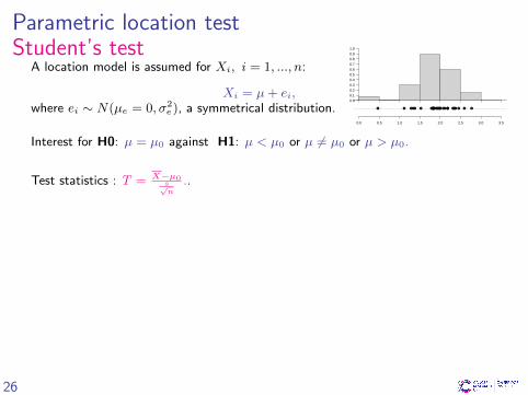
Parametric location testStudent’s test

A location model is assumed for Xi, i = 1, ..., n:

Xi = µ+ ei,where ei ∼ N(µe = 0, σ2

e), a symmetrical distribution.

Interest for H0: µ = µ0 against H1: µ < µ0 or µ 6= µ0 or µ > µ0.

Test statistics : T = X−µ0s√n

..

Distribution of W under H0: T ∼ Student(df = n− 1).

One Sample t-test

data: golub[1042, gol.fac == "ALL"]t = 4.172, df = 26, p-value = 0.0002982alternative hypothesis: true mean is not equal to 1.595 percent confidence interval:1.699817 2.087948sample estimates:mean of x1.893883

0.0 0.5 1.0 1.5 2.0 2.5 3.0 3.5

0.00.10.20.30.40.50.60.70.80.91.0

● ● ●●● ● ●●●●●●●●●●● ●● ●● ●●● ● ● ●

26

Non-parametric location testWilcoxon sign-rank test

A location model is assumed for Xi, i = 1, ..., n:

Xi = θ + ei,where ei ∼ iid(µe = 0, σ2

e), a symmetrical distribution.

Interest for H0: θ = θ0 against H1: θ < θ0 or θ 6= θ0 or θ > θ0.

Test statistics : W+ =∑ni=1 ι(Xi − θ0 > 0) Rank(|Xi − θ0|).

Distribution of W under H0: W+ has no closed-form distribution.

Wilcoxon signed rank exact test

data: golub[1042, gol.fac == "ALL"]V = 333, p-value = 0.0002363alternative hypothesis: true location is not equal to 1.595 percent confidence interval:1.73868 2.09106sample estimates:(pseudo)median

1.926475

0.0 0.5 1.0 1.5 2.0 2.5 3.0 3.5

0.00.10.20.30.40.50.60.70.80.91.0

● ● ●●● ● ●●●●●●●●●●● ●● ●● ●●● ● ● ●

27

Parametric or non-parametric ?

T-test Outcome(s) normally distributed

Yes Mildly No

Sample size

Small

Medium

Large

Situations which may suggest the use of non-parametric statistics:I When there is a small sample size or very unequal groups,I When the data has notable outliers,I When one outcome has a distribution other than normal,I When the data are ordered with many ties or are rank ordered.

Non-parametric does not mean assumption free

28

Introduction to Shiny Apps and Exercises

29

PART III:Parametric and non-parametrictwo-sample location tests

Cancer Research UK – 9th of November 2021D.-L. Couturier (Bioinformatics core)


Two-sample case

Many options:

I One-sided versus two-sided tests,

I Exact versus asymptotic tests,

I Parametric versus non-parametric tests,

I Tests for paired versus independent data.

31

Parametric two-sample location testTwo-sample two-sided Student-s & Welch’s t-tests

●●●

●

Intensity expression of gene 'CCND3 Cyclin D3'

−0.5 0.0 0.5 1.0 1.5 2.0 2.5

Acute lymphoblasticleukemia (ALL)

n=27

Acute myeloidleukemia (AML)

n=11

We test H0: µY − µX = 0 against H1: µY − µX 6= 0.

We know:

I Student’s t-test [assume σ2X = σ2

Y ]: (Y−X)−(µY −µX )

sp

√1nX

+ 1nY

∼ t1−α2,nX+nY −2

I Welch’s t-test [assume σ2X 6= σ2

Y ]: (Y−X)−(µY −µX )√s2XnX

+s2YnY

∼ t1−α2,df

32


●●●

●


−0.5 0.0 0.5 1.0 1.5 2.0 2.5


n=27


n=11


We know:


Y ]: (Y−X)−(µY −µX )

sp

√1nX

+ 1nY

∼ t1−α2,nX+nY −2



+s2YnY

∼ t1−α2,df

Two Sample t-test

data: golub[1042, gol.fac == "ALL"] and golub[1042, gol.fac == "AML"]t = 6.7983, df = 36, p-value = 6.046e-08alternative hypothesis: true difference in means is not equal to 095 percent confidence interval:0.8829143 1.6336690sample estimates:mean of x mean of y1.8938826 0.6355909

32


●●●

●


−0.5 0.0 0.5 1.0 1.5 2.0 2.5


n=27


n=11


We know:


Y ]: (Y−X)−(µY −µX )

sp

√1nX

+ 1nY

∼ t1−α2,nX+nY −2



+s2YnY

∼ t1−α2,df

Welch Two Sample t-test

data: golub[1042, gol.fac == "ALL"] and golub[1042, gol.fac == "AML"]t = 6.3186, df = 16.118, p-value = 9.871e-06alternative hypothesis: true difference in means is not equal to 095 percent confidence interval:0.8363826 1.6802008sample estimates:mean of x mean of y1.8938826 0.6355909

32

Non-parametric two-sample location testMann-Whitney-Wilcoxon test

LetI Xi ∼ iid(µX , σ2), i = 1, ..., nX ,I Yi ∼ iid(µX + δ, σ2), i = 1, ..., nY .

Interest for H0: δ = δ0 against H1: δ < δ0 or δ 6= δ0 or δ > δ0.

Standardised test statistic: z =∑nYi=1

R(Yi)−[nY (nX+nY +1)/2]√nXnY (nX+nY +1)/12

,

where R(Yi) denotes the rank of Yi amongst the combined samples, i.e.,amongst (X1, ..., XnX , Y1, ..., YnY ).

Distribution of Z under H0: Z ∼ N(0, 1).

Implementation 1:statistic = -4.361334 , p-value = 1.292716e-05

Implementation 2:W = 284, p-value = 6.15e-07alternative hypothesis: true location shift is not equal to 095 percent confidence interval:0.89647 1.57023sample estimates:difference in location

1.21951

●●●

●


−0.5 0.0 0.5 1.0 1.5 2.0 2.5


n=27


n=11

33

Non-parametric two-sample location testMann-Whitney-Wilcoxon test

LetI Xi ∼ iid(µX , σ2), i = 1, ..., nX ,I Yi ∼ iid(µX + δ, σ2), i = 1, ..., nY .

Interest for H0: δ = δ0 against H1: δ < δ0 or δ 6= δ0 or δ > δ0.

Standardised test statistic: z =∑nYi=1

R(Yi)−[nY (nX+nY +1)/2]√nXnY (nX+nY +1)/12

,

where R(Yi) denotes the rank of Yi amongst the combined samples, i.e.,amongst (X1, ..., XnX , Y1, ..., YnY ).

Distribution of Z under H0: Z ∼ N(0, 1).

Implementation 1:statistic = -4.361334 , p-value = 1.292716e-05

Implementation 2:W = 284, p-value = 6.15e-07alternative hypothesis: true location shift is not equal to 095 percent confidence interval:0.89647 1.57023sample estimates:difference in location

1.21951

●●●

●


−0.5 0.0 0.5 1.0 1.5 2.0 2.5


n=27


n=11

Den

sity

−4 −3 −2 −1 0 1 2 3 4

0.0

0.1

0.2

0.3

0.4

33

F-test of equality of variances

●●●

●


−0.5 0.0 0.5 1.0 1.5 2.0 2.5


n=27


n=11

We test H0: σ2Y = σ2

X against H1: σ2Y 6= σ2

X .

We know:

I F-test [assume Xi ∼ N(µX , σX) and Yi ∼ N(µY , σY )]:s2Ys2X

∼ FnY −1,nX−1

34

F-test of equality of variances

●●●

●


−0.5 0.0 0.5 1.0 1.5 2.0 2.5


n=27


n=11

We test H0: σ2Y = σ2

X against H1: σ2Y 6= σ2

X .

We know:

I F-test [assume Xi ∼ N(µX , σX) and Yi ∼ N(µY , σY )]:s2Ys2X

∼ FnY −1,nX−1

F test to compare two variances

data: golub[1042, gol.fac == "ALL"] and golub[1042, gol.fac == "AML"]F = 0.71164, num df = 26, denom df = 10, p-value = 0.4652alternative hypothesis: true ratio of variances is not equal to 195 percent confidence interval:0.2127735 1.8428387sample estimates:ratio of variances

0.7116441

34

WarningMultiplicity correction

For each test, the probability of rejecting H0 (and accept H1) when H0 istrue equals α.

For k tests, the probability of rejecting H0 (and accept H1) at least 1 timewhen H0 is true, αk, is given by

αk = 1− (1− α)k.

Thus, for α = 0.05,I if k = 1, α1 = 1− (1− α)1 = 0.05,I if k = 2, α2 = 1− (1− α)2 = 0.0975,I if k = 10, α10 = 1− (1− α)10 = 0.4013.

Idea: change the level of each test so that αk = 0.05:

I Bonferroni correction : α = αkk ,

I Dunn-Sidak correction: α = 1− (1− αk)1/k.

35

WarningNon-parametric is not assumption free: Type I error

Simulate 2500 samples withI Xi ∼ Uniform(1.5, 2.5), i = 1, ..., nX ,I Yi ∼ Uniform(0, 4), i = 1, ..., nY ,

so that E[Xi] = E[Yi] = 2 (i.e., same mean, same median).

AssumeI Xi ∼ iid(µX , σ2), i = 1, ..., nX ,I Yi ∼ iid(µX + δ, σ2), i = 1, ..., nY .

Test H0: δ = δ0 against H1: δ 6= δ0, at the 5% level, by means ofI Mann-Whitney-Wilcoxon test (MWW),I T-test,I Welch-test.

α Tests

MWW Student’s t-test Welch’s test

Sample size nX = 200, nY = 70 0.145 0.202 0.055

nX = 20, nY = 7 0.148 0.240 0.062

36

Exercises

37

introduction tostatistical analysis

Documents