introduction to time series mining - didawiki

Introduction to

Time Series Mining

Slides from Keogh

Eamonn’s tutorial:

• Introduction, Motivation

• The Utility of Similarity Measurements• Properties of distance measures

• The Euclidean distance

• Preprocessing the data

• Dynamic Time Warping

• Uniform Scaling

• Indexing Time Series• Spatial Access Methods and the curse of

dimensionality

• The GEMINI Framework

• Dimensionality reduction• Discrete Fourier Transform

• Discrete Wavelet Transform

• Singular Value Decomposition

• Piecewise Linear Approximation

• Symbolic Approximation

• Piecewise Aggregate Approximation

• Adaptive Piecewise Constant Approximation

• Empirical Comparison

Outline of TutorialOutline of Tutorial

• Data Mining• Anomaly/Interestingness detection

• Motif (repeated pattern) discovery

• Visualization/Summarization

• What we should be working on!

Summary, Conclusions

What are Time Series?What are Time Series?

0 50 100 150 200 250 300 350 400 450 50023

24

25

26

27

28

29

25.1750

25.2250

25.2500

25.2500

25.2750

25.3250

25.3500

25.3500

25.4000

25.4000

25.3250

25.2250

25.2000

25.1750

..

..24.6250

24.6750

24.6750

24.6250

24.6250

24.6250

24.6750

24.7500

25.1750

25.2250

25.2500

25.2500

25.2750

25.3250

25.3500

25.3500

25.4000

25.4000

25.3250

25.2250

25.2000

25.1750

..

..24.6250

24.6750

24.6750

24.6250

24.6250

24.6250

24.6750

24.7500

A time series is a collection of observations made

sequentially in time.

Virtually all similarity measurements, indexing and dimensionality reduction techniques discussed in this tutorial can be used with other data types

Virtually all similarity measurements, indexing and dimensionality reduction techniques discussed in this tutorial can be used with other data types

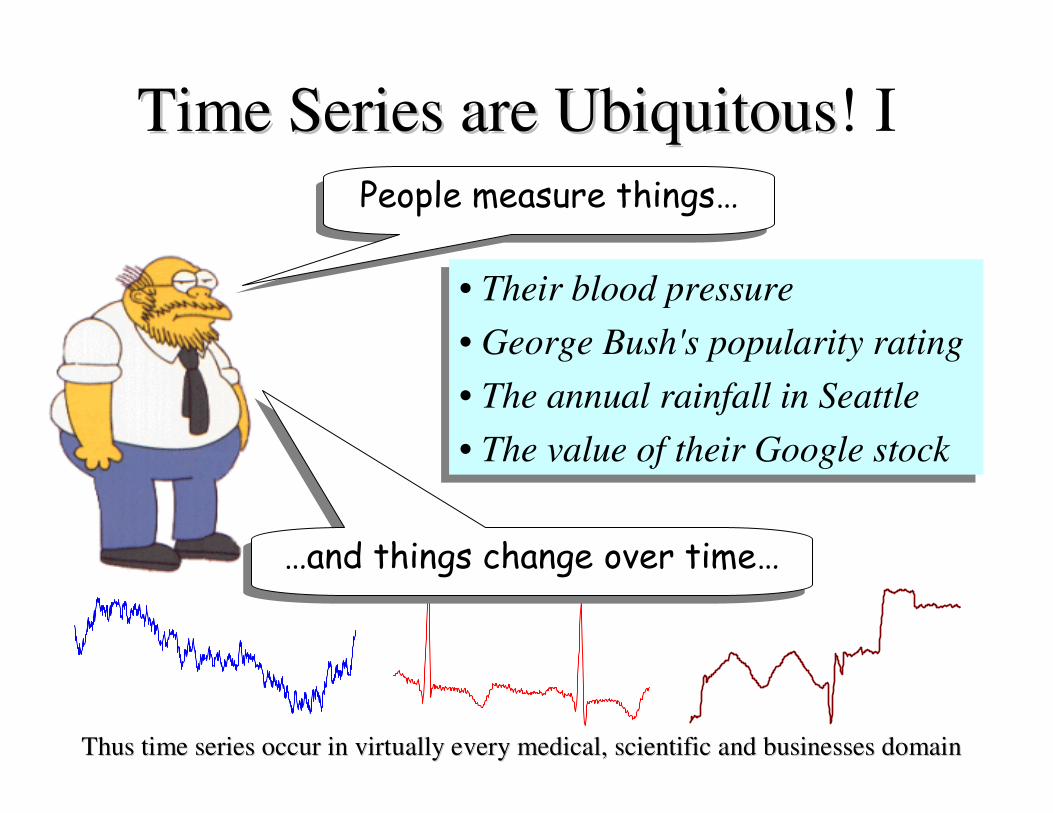
Time Series are UbiquitousTime Series are Ubiquitous! I

• Their blood pressure

• George Bush's popularity rating

• The annual rainfall in Seattle

• The value of their Google stock

• Their blood pressure

• George Bush's popularity rating

• The annual rainfall in Seattle

• The value of their Google stock

Thus time series occur in virtually every medical, scientific anThus time series occur in virtually every medical, scientific and businesses domaind businesses domain

People measure things…People measure things…

…and things change over time……and things change over time…

Image data, may best be thought of as time series…Image data, may best be thought of as time series…

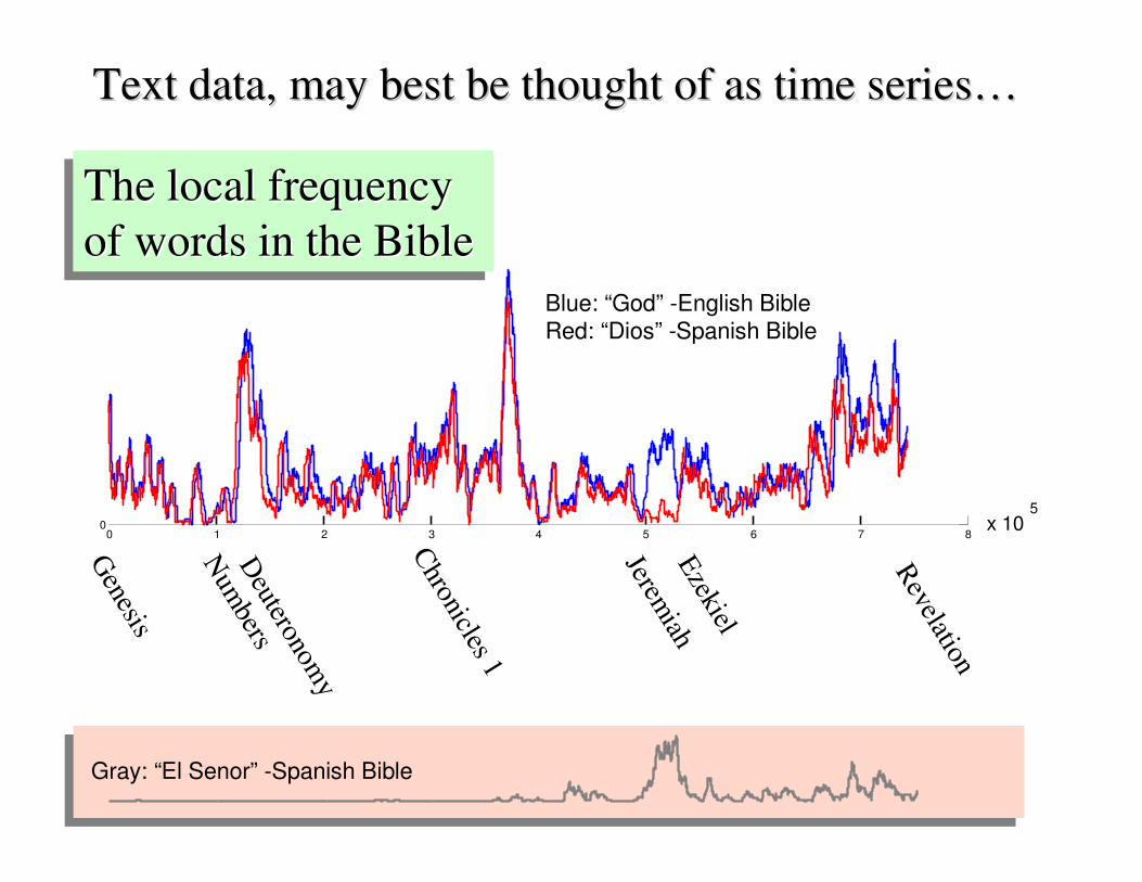
Text data, may best be thought of as time series…Text data, may best be thought of as time series…

0 1 2 3 4 5 6 7 8x 10

50

Blue: “God” -English Bible Red: “Dios” -Spanish Bible

Genesis

Jeremiah

Ezekiel

Revelation

Deuteronom

y

Chronicles 1

Gray: “El Senor” -Spanish Bible

Num

bers

The local frequency

of words in the Bible

The local frequency The local frequency

of words in the Bibleof words in the Bible

0 10 20 30 40 50 60 70 80 90

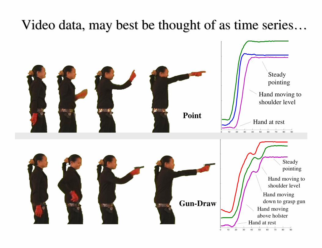
Hand at rest

Hand moving to

shoulder level

Steady

pointing

0 10 20 30 40 50 60 70 80 90

Hand at rest

Hand moving

above holster

Hand moving

down to grasp gun

Hand moving to

shoulder level

Steady

pointing

Video data, may best be thought of as time series…Video data, may best be thought of as time series…

Point

Gun-Draw

Brain scans (3D Brain scans (3D voxelsvoxels), may best be thought of as time series…), may best be thought of as time series…

Wang, Kontos, Li and Megalooikonomou ICASSP 2004

Why is Working With Time Series so Why is Working With Time Series so

Difficult? Part I Difficult? Part I

� 1 Hour of EKG data:1 Hour of EKG data: 1 Gigabyte.

� Typical Typical WeblogWeblog: 5 Gigabytes per week.

� Space Shuttle DatabaseSpace Shuttle Database: 200 Gigabytes and growing.

� Macho DatabaseMacho Database: 3 Terabytes, updated with 3 gigabytes a day.

Answer:Answer: How do we work with very large databases?How do we work with very large databases?

Since most of the data lives on disk (or tape), we need a

representation of the data we can efficiently manipulate.

Why is Working With Time Series so Why is Working With Time Series so

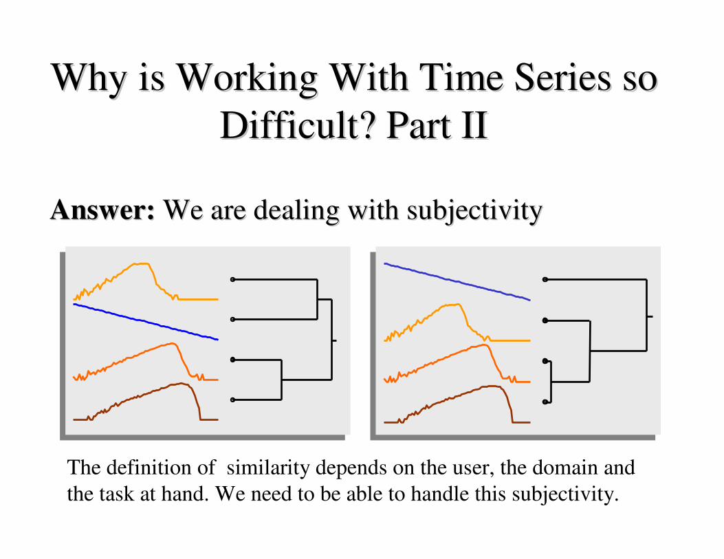
Difficult? Part II Difficult? Part II

The definition of similarity depends on the user, the domain and

the task at hand. We need to be able to handle this subjectivity.

Answer:Answer: We are dealing with subjectivityWe are dealing with subjectivity

Why is working with time series so Why is working with time series so

difficult? Part III difficult? Part III

Answer:Answer: Miscellaneous data handling problems.Miscellaneous data handling problems.

•• Differing data formats.Differing data formats.

•• Differing sampling rates.Differing sampling rates.

•• Noise, missing values, etc.Noise, missing values, etc.

We will not focus on these issues in this tutorial.

What do we want to do with the time series data?What do we want to do with the time series data?

ClusteringClustering ClassificationClassification

Query by

ContentRule

Discovery10

⇒s = 0.5

c = 0.3

Motif DiscoveryMotif Discovery

Novelty DetectionNovelty DetectionVisualizationVisualization

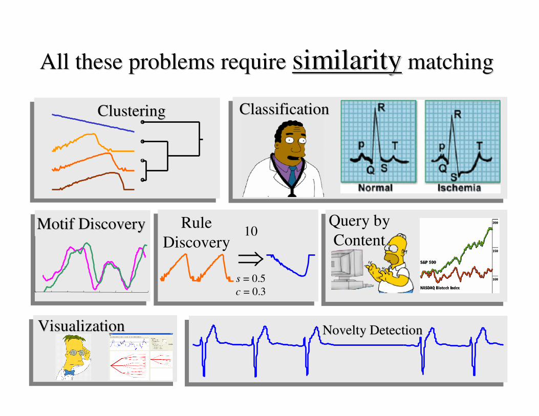
All these problems require All these problems require similaritysimilarity matchingmatching

ClusteringClustering ClassificationClassification

Query by

ContentRule

Discovery10

⇒s = 0.5

c = 0.3

Motif DiscoveryMotif Discovery

Novelty DetectionNovelty DetectionVisualizationVisualization

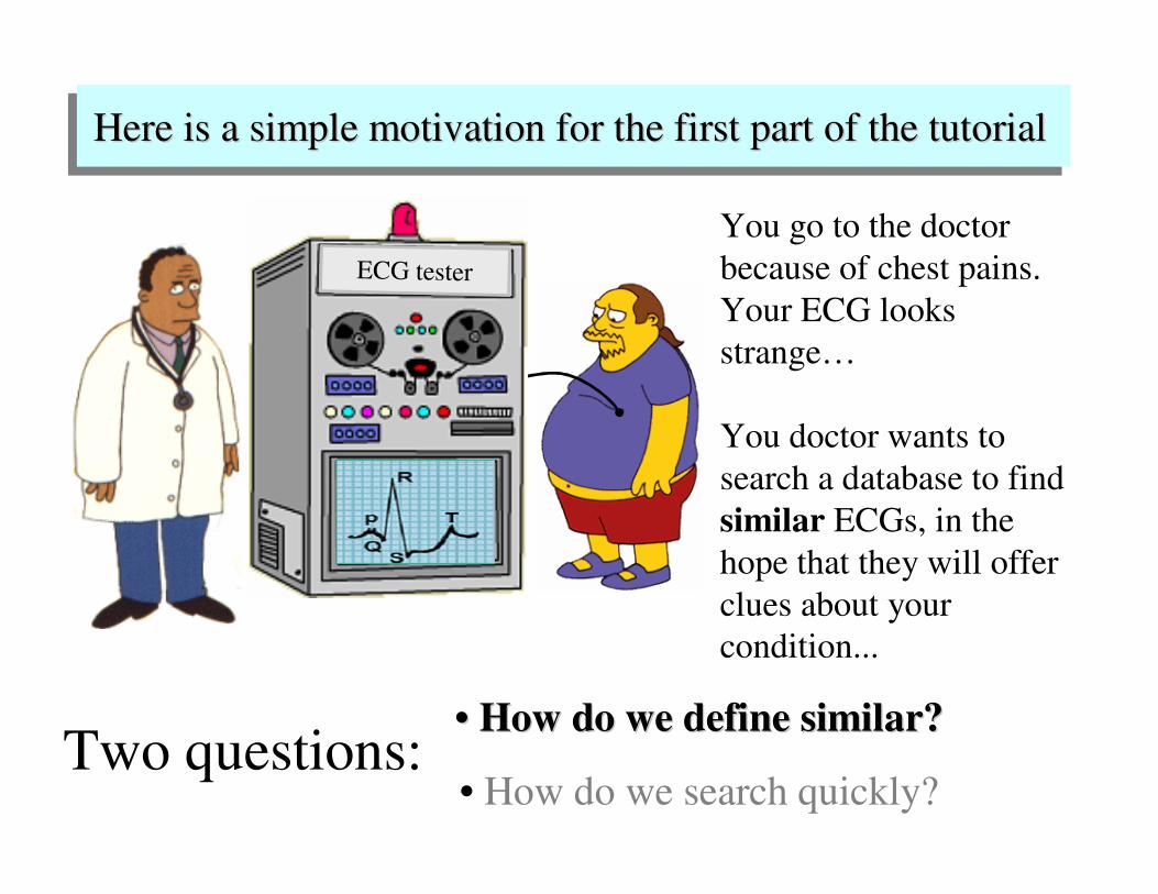
Here is a simple motivation for the first part of the tutorialHere is a simple motivation for the first part of the tutorial

You go to the doctor

because of chest pains.

Your ECG looks

strange…

You doctor wants to

search a database to find

similar ECGs, in the

hope that they will offer

clues about your

condition...

Two questions:•• How do we define similar?How do we define similar?

• How do we search quickly?

ECG tester

What is Similarity?What is Similarity?The quality or state of being similar; likeness;

resemblance; as, a similarity of features.

Similarity is hard to

define, but…

“We know it when we

see it”

The real meaning of

similarity is a

philosophical question.

We will take a more

pragmatic approach.

Webster's Dictionary

Two Kinds of SimilarityTwo Kinds of SimilaritySimilarity at the level of

shapeNext 40 minutes

Similarity at the level of

shapeNext 40 minutes

Similarity at the structural

levelAnother 10 minutes

Similarity at the structural

levelAnother 10 minutes

time series

( ) ( )∑ −≡=

n

iii cqCQD

1

2,

Q

C

D(Q,C)

Euclidean Distance MetricEuclidean Distance Metric

About 80% of published work in data mining uses

Euclidean distance

About 80% of published work in data mining uses

Euclidean distance

Given two time series:

Q = q1…qn

C = c1…cn

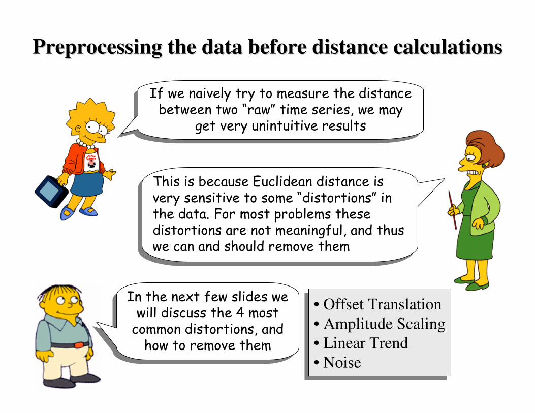
In the next few slides we will discuss the 4 most common distortions, and how to remove them

In the next few slides we will discuss the 4 most common distortions, and how to remove them

Preprocessing the data before distance calculationsPreprocessing the data before distance calculations

• Offset Translation

• Amplitude Scaling

• Linear Trend

• Noise

This is because Euclidean distance is very sensitive to some “distortions” in the data. For most problems these distortions are not meaningful, and thus we can and should remove them

This is because Euclidean distance is very sensitive to some “distortions” in the data. For most problems these distortions are not meaningful, and thus we can and should remove them

If we naively try to measure the distance between two “raw” time series, we may

get very unintuitive results

If we naively try to measure the distance between two “raw” time series, we may

get very unintuitive results

Transformation I: Offset TranslationTransformation I: Offset Translation

0 50 100 150 200 250 3000

0.5

1

1.5

2

2.5

3

0 50 100 150 200 250 3000

0.5

1

1.5

2

2.5

3

0 50 100 150 200 250 3000 50 100 150 200 250 300

Q = Q - mean(Q)

C = C - mean(C)

D(Q,C)

D(Q,C)

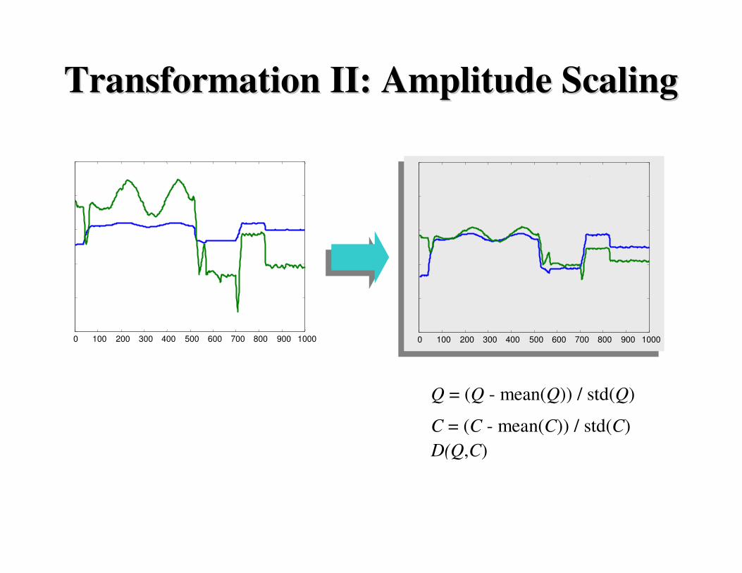
Transformation II: Amplitude ScalingTransformation II: Amplitude Scaling

0 100 200 300 400 500 600 700 800 900 1000 0 100 200 300 400 500 600 700 800 900 1000

Q = (Q - mean(Q)) / std(Q)

C = (C - mean(C)) / std(C)

D(Q,C)

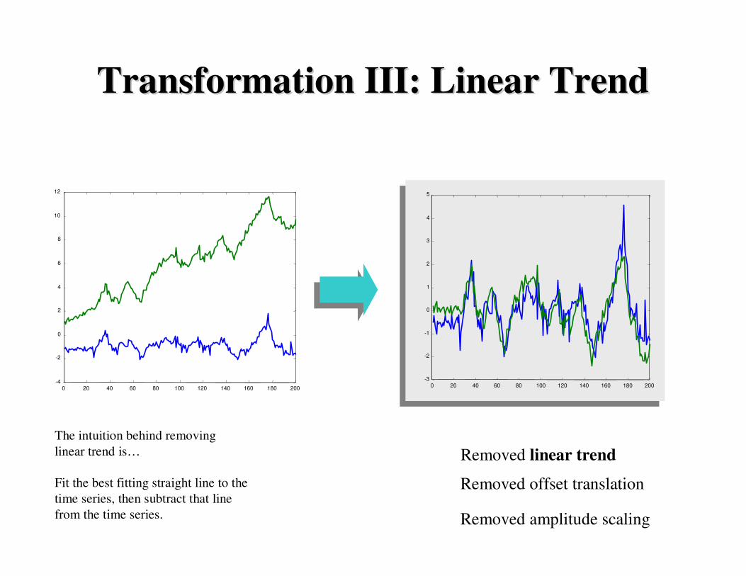
Transformation III: Linear TrendTransformation III: Linear Trend

0 20 40 60 80 100 120 140 160 180 200-4

-2

0

2

4

6

8

10

12

0 20 40 60 80 100 120 140 160 180 200-3

-2

-1

0

1

2

3

4

5

Removed offset translation

Removed amplitude scaling

Removed linear trend

The intuition behind removing

linear trend is…

Fit the best fitting straight line to the

time series, then subtract that line

from the time series.

Transformation IIII: NoiseTransformation IIII: Noise

0 20 40 60 80 100 120 140-4

-2

0

2

4

6

8

0 20 40 60 80 100 120 140-4

-2

0

2

4

6

8

Q = smooth(Q)

C = smooth(C)

D(Q,C)

The intuition behind

removing noise is...

Average each datapoints

value with its neighbors.

1

2

3

4

6

5

7

8

9

A Quick Experiment to Demonstrate the A Quick Experiment to Demonstrate the

Utility of Preprocessing the DataUtility of Preprocessing the Data

1

4

7

5

8

6

9

2

3

Clustered using Euclidean distance, after removing

noise, linear trend, offset translation and

amplitude scaling

Clustered using Euclidean distance, after removing

noise, linear trend, offset translation and

amplitude scaling

Clustered using Euclidean

distance on the raw data.

Clustered using Euclidean

distance on the raw data.

Summary of PreprocessingSummary of Preprocessing

We should keep in mind these problems as we consider the high level representations of time series which we will encounter later (DFT, Wavelets etc). Since these representations often allow us to handle distortions in elegant ways

We should keep in mind these problems as we consider the high level representations of time series which we will encounter later (DFT, Wavelets etc). Since these representations often allow us to handle distortions in elegant ways

Of course, sometimes the distortions are the most interesting thing about the data, the above is only a general rule

Of course, sometimes the distortions are the most interesting thing about the data, the above is only a general rule

The “raw” time series may have distortions which we should remove before clustering, classification etc

The “raw” time series may have distortions which we should remove before clustering, classification etc

Fixed Time AxisSequences are aligned “one to one”.

“Warped” Time AxisNonlinear alignments are possible.

Dynamic Time WarpingDynamic Time Warping

Note: We will first see the utility of DTW, then see how it is calculated.

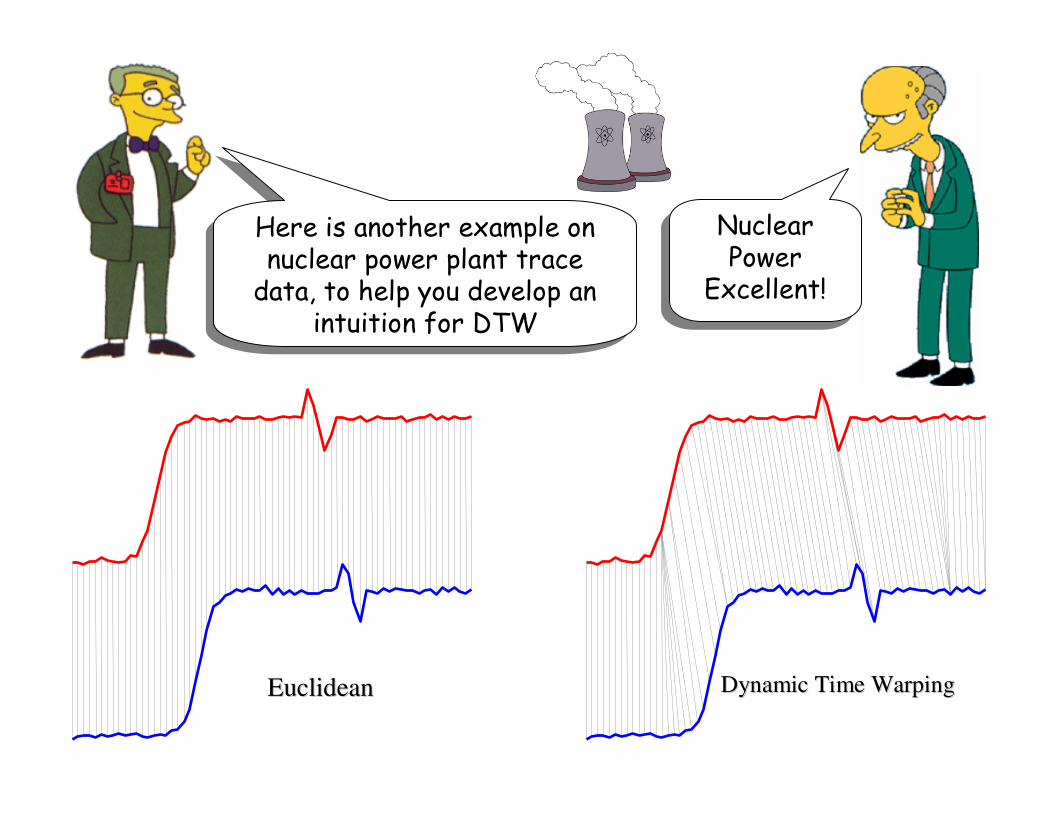
EuclideanEuclidean Dynamic Time WarpingDynamic Time Warping

Nuclear Power

Excellent!

Nuclear Power

Excellent!

Here is another example on nuclear power plant trace data, to help you develop an

intuition for DTW

Here is another example on nuclear power plant trace data, to help you develop an

intuition for DTW

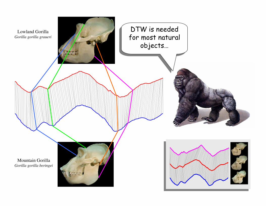
Mountain GorillaGorilla gorilla beringei

Lowland GorillaGorilla gorilla graueri

DTW is needed for most natural

objects…

DTW is needed for most natural

objects…

0 10 20 30 40 50 60 70 80 900 10 20 30 40 50 60 70 80

-4

-3

-2

-1

0

1

2

3

4

Sign language

0 50 100 150 200 250 300-3

-2

-1

0

1

2

3

4

Trace

Word Spotting

Gun

Let us compare Euclidean Distance and DTW on some problemsLet us compare Euclidean Distance and DTW on some problems

Faces

Leaves

Control

2-Patterns

0.001.042-Patterns

0.337.5Control Chart*

2.686.25(4) Faces

4.0733.26Leaves#

0.0011.00Nuclear Trace

1.005.50GUN

25.9328.70Sign language

1.104.78Word Spotting

DTWDTWEuclideanEuclideanDatasetDataset

Results: Error RateResults: Error Rate

Using 1-nearest-neighbor, leaving-one-out

evaluation!

Using 1-nearest-neighbor, leaving-one-out

evaluation!

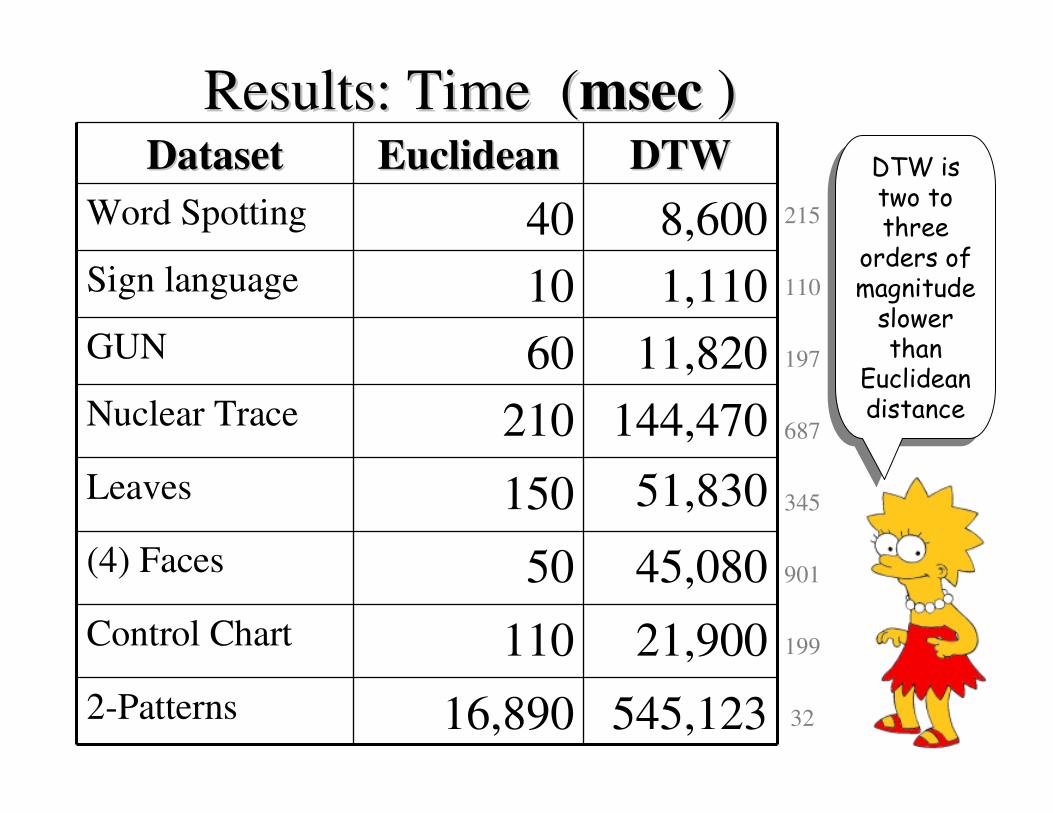
545,12316,8902-Patterns

21,900110Control Chart

45,08050(4) Faces

51,830150Leaves

144,470210Nuclear Trace

11,82060GUN

1,11010Sign language

8,60040Word Spotting

DTWDTWEuclideanEuclideanDatasetDataset

Results: Time (Results: Time (msecmsec ))

215

110

197

687

345

901

199

32

DTW is two to three

orders of magnitude slower than

Euclidean distance

DTW is two to three

orders of magnitude slower than

Euclidean distance

C

QC

Q

How is DTW How is DTW

Calculated? ICalculated? I

We create a matrix the size of

|Q| by |C|, then fill it in with the

distance between every pair of

point in our two time series.

C

Q

C

Q

How is DTW How is DTW

Calculated? IICalculated? II= ∑ =

KwCQDTWK

k k1min),(

Warping path w

Every possible warping between two time

series, is a path though the matrix. We

want the best one…

γ(i,j) = d(qi,cj) + min{ γ(i-1,j-1), γ(i-1,j ), γ(i,j-1) }

This recursive function gives us the

minimum cost path

Let us visualize the cumulative matrix on a real world problem ILet us visualize the cumulative matrix on a real world problem I

This example shows 2

one-week periods from

the power demand time

series.

Note that although they

both describe 4-day work

weeks, the blue sequence

had Monday as a holiday,

and the red sequence had

Wednesday as a holiday.

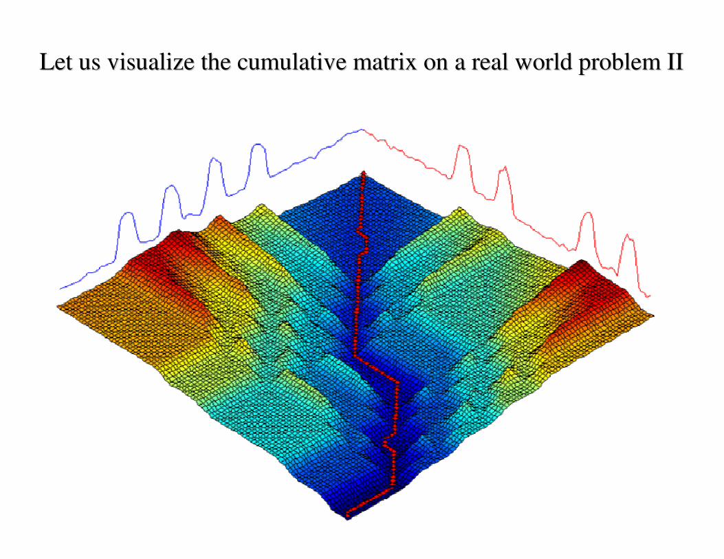
Let us visualize the cumulative matrix on a real world problem ILet us visualize the cumulative matrix on a real world problem III

What we have seen so far…What we have seen so far…

• Dynamic Time Warping gives

much better results than

Euclidean distance on virtually

all problems.

• Dynamic Time Warping is

very very slow to calculate!

Is there anything we can do to speed up similarity search under DTW?

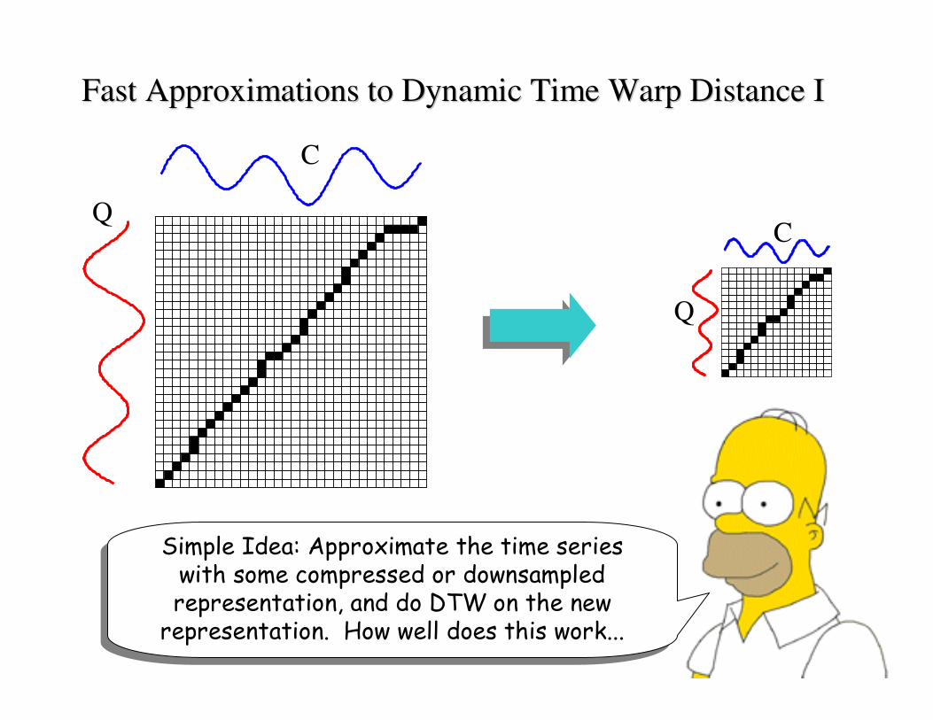
Fast Approximations to Dynamic Time Warp Distance IFast Approximations to Dynamic Time Warp Distance I

C

QC

Q

Simple Idea: Approximate the time series with some compressed or downsampledrepresentation, and do DTW on the new representation. How well does this work...

Simple Idea: Approximate the time series with some compressed or downsampledrepresentation, and do DTW on the new representation. How well does this work...

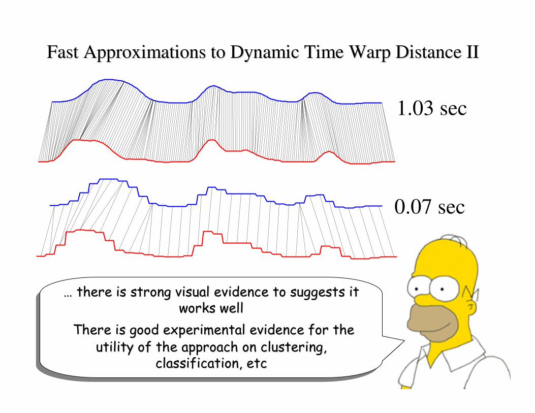
Fast Approximations to Dynamic Time Warp Distance IIFast Approximations to Dynamic Time Warp Distance II

0.07 sec

1.03 sec

… there is strong visual evidence to suggests it works well

There is good experimental evidence for the utility of the approach on clustering,

classification, etc

…… there is strong visual evidence to suggests it there is strong visual evidence to suggests it works wellworks well

There is good experimental evidence for the There is good experimental evidence for the utility of the approach on clustering, utility of the approach on clustering,

classification, etcclassification, etc

C

Q

C

Q

Sakoe-Chiba Band Itakura Parallelogram

Global Global ConstraintsConstraints

• Slightly speed up the calculations

• Prevent pathological warpings

65

70

75

80

85

90

95

100

1 5 9

13

17

21

25

29

33

37

41

45

49

53

57

61

65

69

73

77

81

85

89

93

97

100

FACE 2%

GUNX 3%

LEAF 8%

Control Chart 4%

TRACE 3%

2-Patterns 3%

WordSpotting 3%

Warping width that achieves

max Accuracy

Accu

racy

W: Warping Width

W

Accuracy vs. Width of Warping WindowAccuracy vs. Width of Warping Window

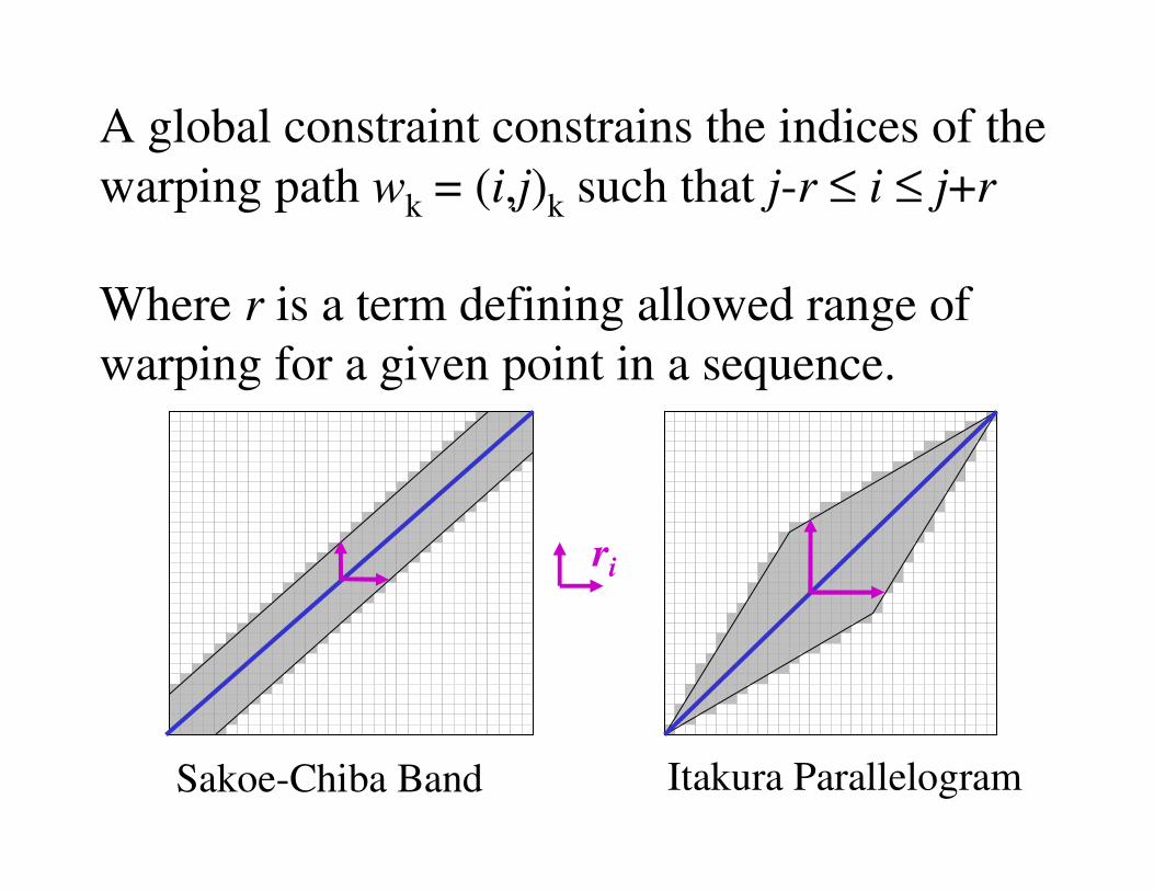
A global constraint constrains the indices of the

warping path wk = (i,j)k such that j-r ≤ i ≤ j+r

Where r is a term defining allowed range of

warping for a given point in a sequence.

ri

Sakoe-Chiba Band Itakura Parallelogram

In general, it’s hard to speed up a single DTW calculationIn general, itIn general, it’’s hard to speed up a single DTW calculations hard to speed up a single DTW calculation

However, if we have to make many DTW calculations (which is almost always the case), we can potentiality speed up the

whole process by lowerbounding.

However, if we have to make many DTW However, if we have to make many DTW calculations (which is almost always the calculations (which is almost always the case), we can potentiality speed up the case), we can potentiality speed up the

whole process by whole process by lowerboundinglowerbounding. .

Keep in mind that the lowerbounding trick works for any situation were you have an

expensive calculation that can be lowerbounded(string edit distance, graph edit distance etc)

Keep in mind that the Keep in mind that the lowerboundinglowerbounding trick trick works for any situation were you have an works for any situation were you have an

expensive calculation that can be expensive calculation that can be lowerboundedlowerbounded(string edit distance, graph edit distance etc)(string edit distance, graph edit distance etc)

I will explain how lowerbounding works in a generic fashion in the next two slides, then show concretely how lowerbounding makes dealing with massive time series under DTW possible…

I will explain how I will explain how lowerboundinglowerbounding works in a works in a generic fashion in the next two slides, then show generic fashion in the next two slides, then show concretely how concretely how lowerboundinglowerbounding makes dealing makes dealing with massive time series under DTW possiblewith massive time series under DTW possible……

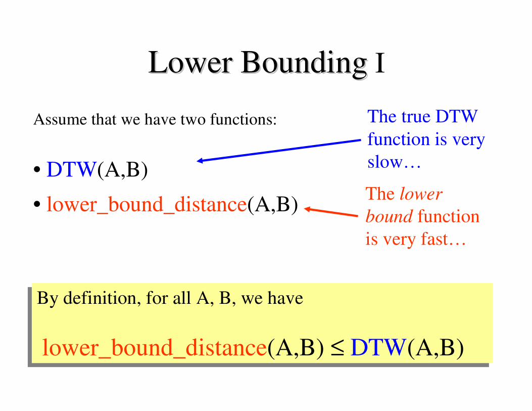
Lower BoundingLower Bounding I

Assume that we have two functions:

• DTW(A,B)

• lower_bound_distance(A,B)

The true DTW

function is very

slow…

The lower

bound function

is very fast…

By definition, for all A, B, we have

lower_bound_distance(A,B) ≤ DTW(A,B)

By definition, for all A, B, we have

lower_bound_distance(A,B) ≤ DTW(A,B)

Lower BoundingLower Bounding II

1. best_so_far = infinity;

2. for all sequences in database

3. LB_dist = lower_bound_distance(

4. if LB_dist < best_so_far

5. true_dist = DTW(

6. if true_dist < best_so_far

7. best_so_far = true_dist;

8. index_of_best_match = i;

9. endif

10. endif

11. endfor

Algorithm Lower_Bounding_Sequential_Scan(Q)

1. best_so_far = infinity;

2. for all sequences in database

3.

4. if LB_dist < best_so_far

5. Ci, Q);Ci, Q);

6. if true_dist < best_so_far

7. best_so_far = true_dist;

8. index_of_best_match = i;

9. endif

10. endif

11. endfor

Algorithm Lower_Bounding_Sequential_Scan(Q)

We can speed up similarity search under DTW

by using a lower bounding function

Ci, Q);Ci, Q);

Only do the expensive, full calculations when it is absolutely necessary

Only do the expensive, full calculations when it is absolutely necessary

Try to use a cheap lower bounding calculation as often as possible.

Try to use a cheap lower bounding calculation as often as possible.

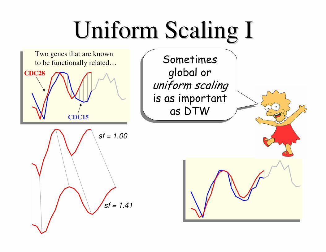
Uniform Scaling IUniform Scaling I

sf = 1.00

sf = 1.41

CDC28

CDC15

Two genes that are known

to be functionally related… Sometimes global or

uniform scalingis as important

as DTW

Sometimes global or

uniform scalingis as important

as DTW

sf = 1.00

sf = 1.01

sf = 1.10

1

23

0 200 400 600 800 1000

2

1

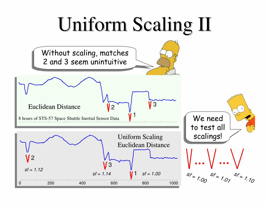
3sf = 1.12

sf = 1.14 sf = 1.00

Euclidean DistanceEuclidean Distance

Uniform Scaling Uniform Scaling

Euclidean DistanceEuclidean Distance

Uniform Scaling IIUniform Scaling II

8 hours of STS-57 Space Shuttle Inertial Sensor Data

… …

We need to test all scalings!

We need to test all scalings!

Without scaling, matches 2 and 3 seem unintuitive

Without scaling, matches 2 and 3 seem unintuitive

Algorithm: Test_All_Scalings(Q,C)

best_match_val = inf;

best_scaling_factor = null;for p = n to m

QP = rescale(Q,p);distance = squared_Euclidean_distance(QP, C[1..p]);if distance < best_match_val

best_match_val = distance;best_scaling_factor = p/n;

end;end;

return(best_match_val, best_scaling_factor)

Here is the code to

Test_All_Scalings, the time

complexly is only O((m-n) * n), but we may have to do this many times…

Here is the code to

Test_All_Scalings, the time

complexly is only O((m-n) * n), but we may have to do this many times…

Here is some notation, the shortest scaling we

consider is length n, and the largest is length m.

The scaling factor (sf) is the ratio i/n , n <= i <= m

Here is some notation, the shortest scaling we

consider is length n, and the largest is length m.

The scaling factor (sf) is the ratio i/n , n <= i <= m

n i m

sf = 1.00

sf = 1.05

sf = 1.15

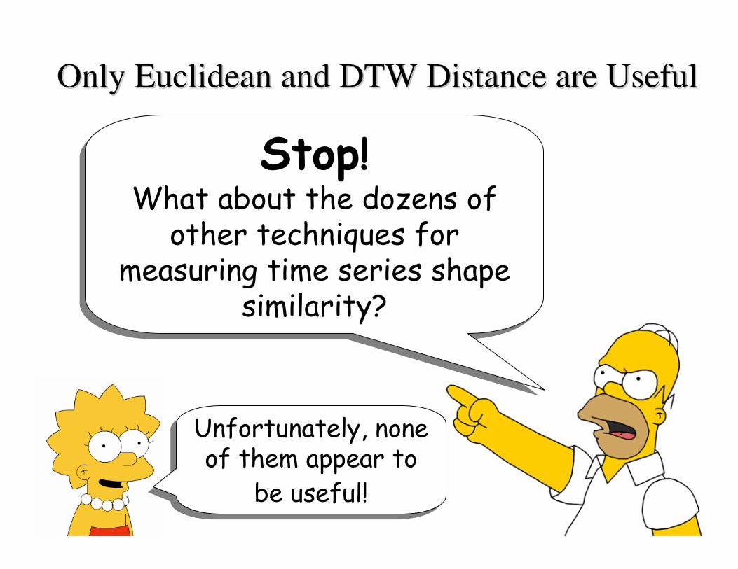
Stop!What about the dozens of

other techniques for measuring time series shape

similarity?

Stop!What about the dozens of

other techniques for measuring time series shape

similarity?

Unfortunately, none of them appear to

be useful!

Unfortunately, none of them appear to

be useful!

Only Euclidean and DTW Distance are UsefulOnly Euclidean and DTW Distance are Useful

0.5930.331Hölder

0.3210.202Piecewise Probabilistic

0.3710.130Cosine Wavelets

0.6950.444String Signature

0.6220.603Edit Distance

0.4780.387Important Points

0.5780.206String (Suffix Tree)

0.4580.570Cepstrum

0.1160.380Autocorrelation Functions

0.3210.130Piecewise Normalization

0.6230.451Aligned Subsequence

0.0130.003Euclidean Distance

Control-ChartCylinder-Bell-F’Approach

Classification Error Rates on Classification Error Rates on two publicly available datasetstwo publicly available datasets

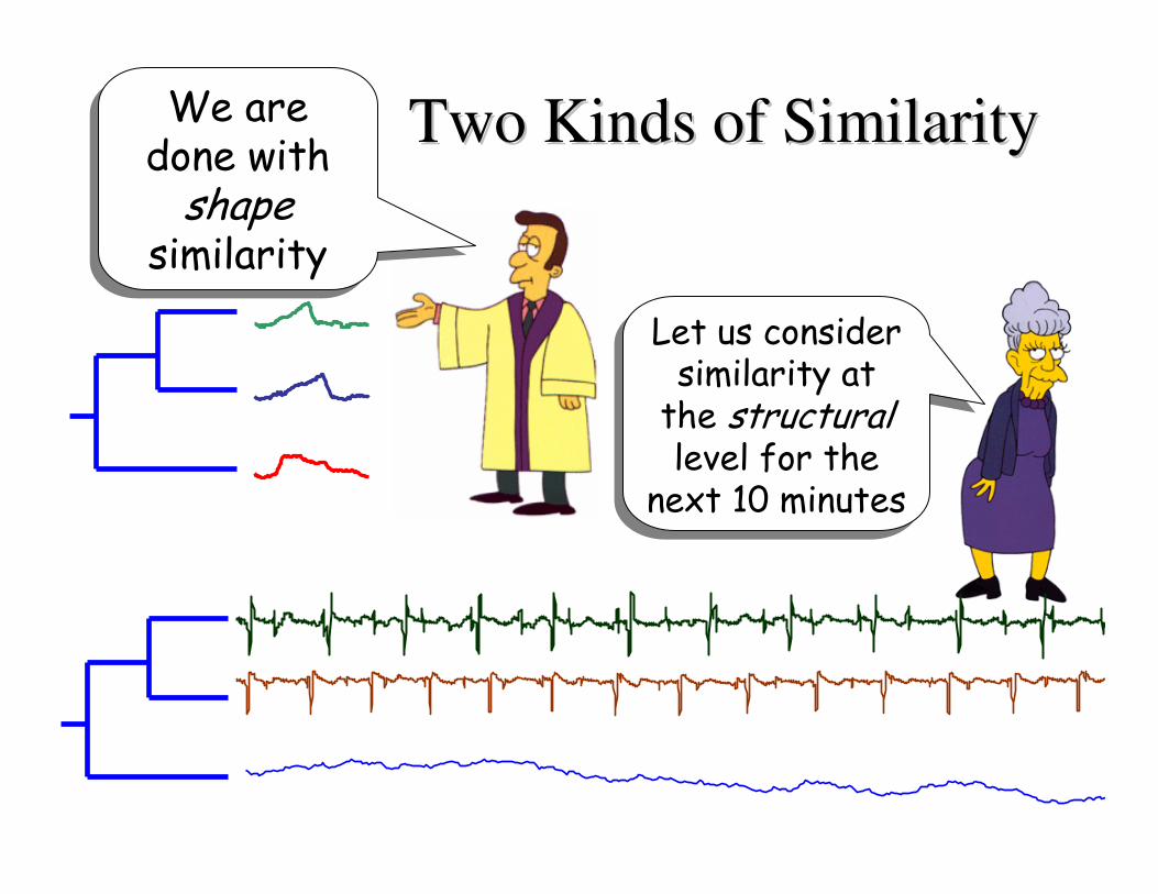
Two Kinds of SimilarityTwo Kinds of SimilarityWe are done with shape

similarity

We are done with shape

similarity

Let us considersimilarity at the structurallevel for the

next 10 minutes

Let us considersimilarity at the structurallevel for the

next 10 minutes

Euclidean

Distance

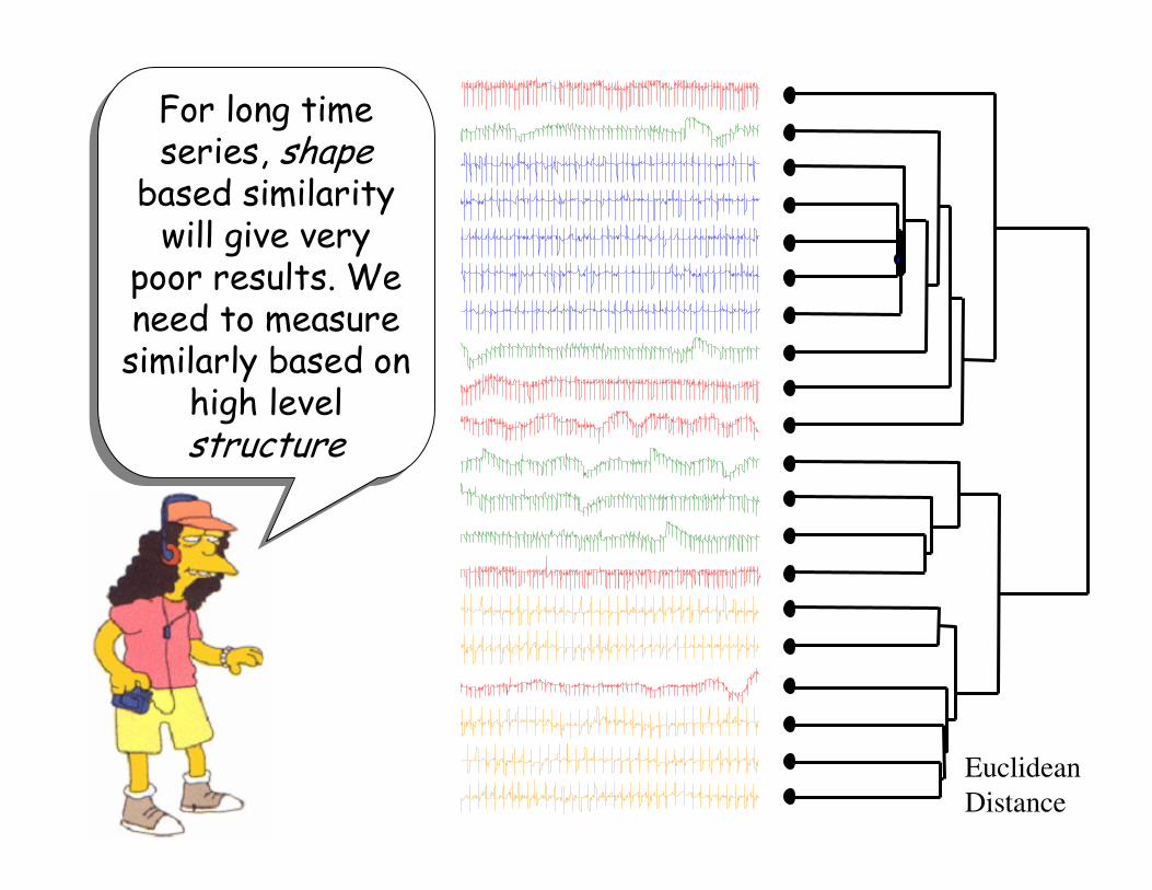
For long time series, shape

based similarity will give very

poor results. We need to measure similarly based on

high level structure

For long time series, shape

based similarity will give very

poor results. We need to measure similarly based on

high level structure

Structure or Model Based SimilarityStructure or Model Based Similarity

A

B

C

…………0.10.40.3ARIMA

138298Zero Crossings

0.50.30.2Autocorrelation

191211Max Value

CBAFeatureFeature

Time Time

SeriesSeries

The basic idea is to extract global features from the time series, create a feature

vector, and use these feature vectors to measure similarity and/or classify

The basic idea is to extract global features from the time series, create a feature

vector, and use these feature vectors to measure similarity and/or classify

But which• features?

• distance measure/

learning algorithm?

But which• features?


learning algorithm?

FeatureFeature--based Classification of Timebased Classification of Time--series Dataseries DataNanopoulos, Alcock, and Manolopoulos

mean (1st derivative)

variance (1st derivative)

skewness (1st derivative)

kurtosis (1st derivative)

kurtosis

skewness

variance

mean

FeaturesFeatures

Learning AlgorithmLearning Algorithmmulti-layer perceptron neural network

• features?


learning algorithm?

• features?


learning algorithm?

Makes sense, but when we looked at the samedataset, we found we

could be better classification accuracy

with Euclidean distance!

Makes sense, but when we looked at the samedataset, we found we

could be better classification accuracy

with Euclidean distance!

Learning to Recognize Time Series: Combining ARMA Models with Learning to Recognize Time Series: Combining ARMA Models with

MemoryMemory--Based LearningBased LearningDeng, Moore and Nechyba

The parameters of the

Box Jenkins model.

More concretely, the

coefficients of the

ARMA model.

FeaturesFeatures

Distance MeasureDistance MeasureEuclidean distance (between coefficients)

“Time series must

be invertible and

stationary”

• features?


learning algorithm?

• features?


learning algorithm?

• Use to detect drunk drivers!

• Independently rediscovered and

generalized by Kalpakis et. al. and

expanded by Xiong and Yeung

Deformable Markov Model Templates for Time Series Pattern MatchiDeformable Markov Model Templates for Time Series Pattern MatchingngGe and Smyth

The parameters of a

Markov Model

The time series is first

converted to a piecewise

linear model

FeaturesFeatures

Distance MeasureDistance Measure“Viterbi-Like” Algorithm

• features?


learning algorithm?

• features?


learning algorithm?

0 20 40 60 80 100 120 140

X

X'

A B C0.30.20.5C

0.20.20.4B

0.50.40.1A

CBA

Variations independently developed by Li and Biswas, Ge and Smyth, Lin, Orgun

and Williams etc

Variations independently developed by Li and Biswas, Ge and Smyth, Lin, Orgun

and Williams etc

There tends to be lots of

parameters to tune…

There tends to be lots of

parameters to tune…

Part 1

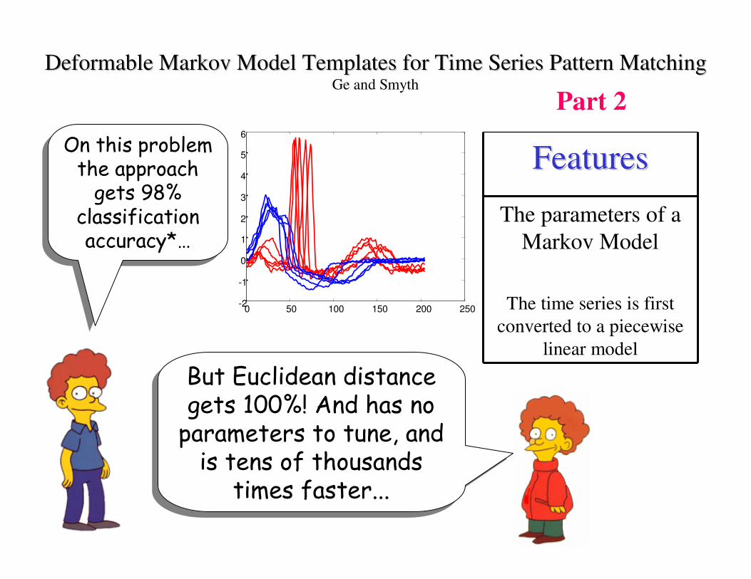
Deformable Markov Model Templates for Time Series Pattern MatchiDeformable Markov Model Templates for Time Series Pattern MatchingngGe and Smyth

The parameters of a

Markov Model

The time series is first

converted to a piecewise

linear model

FeaturesFeaturesOn this problem the approach gets 98%

classification accuracy*…

On this problem the approach gets 98%

classification accuracy*…

Part 2

0 50 100 150 200 250-2

-1

0

1

2

3

4

5

6

But Euclidean distance gets 100%! And has no parameters to tune, and is tens of thousands

times faster...

But Euclidean distance gets 100%! And has no parameters to tune, and is tens of thousands

times faster...

Compression Based DissimilarityCompression Based Dissimilarity(In general) Li, Chen, Li, Ma, and Vitányi: (For time series) Keogh, Lonardi and Ratanamahatana

Whatever structure

the compression

algorithm finds...

The time series is first converted

to the SAX symbolic

representation*

FeaturesFeatures

Distance MeasureDistance MeasureCo-Compressibility

• features?


learning algorithm?

• features?


learning algorithm?

Euclidean CDM

)()(

)(),(

yCxC

xyCyxCDM

+=

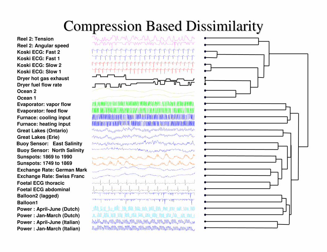
Compression Based DissimilarityCompression Based Dissimilarity

Power : Jan-March (Italian)

Power : April-June (Italian)

Power : Jan-March (Dutch)

Power : April-June (Dutch)

Balloon1

Balloon2 (lagged)

Foetal ECG abdominal

Foetal ECG thoracic

Exchange Rate: Swiss Franc

Exchange Rate: German Mark

Sunspots: 1749 to 1869

Sunspots: 1869 to 1990

Buoy Sensor: North Salinity

Buoy Sensor: East Salinity

Great Lakes (Erie)

Great Lakes (Ontario)

Furnace: heating input

Furnace: cooling input

Evaporator: feed flow

Evaporator: vapor flow

Ocean 1

Ocean 2

Dryer fuel flow rate

Dryer hot gas exhaust

Koski ECG: Slow 1

Koski ECG: Slow 2

Koski ECG: Fast 1

Koski ECG: Fast 2

Reel 2: Angular speed

Reel 2: Tension

Summary of Time Series SimilaritySummary of Time Series Similarity

• If you have short time series, use DTW after

searching over the warping window size1 (and

shape2)

• Then use envelope based lower bounds to speed

things up3.

• If you have long time series, and you know

nothing about your data, try compression based

dissimilarity.

• If you do know something about your data, try to

leverage of this knowledge to extract features.

Motivating example revisited…Motivating example revisited…

You go to the doctor

because of chest pains.

Your ECG looks

strange…

Your doctor wants to

search a database to find

similar ECGs, in the

hope that they will offer

clues about your

condition...

Two questions:•How do we define similar?

••How do we search quickly?How do we search quickly?

ECG

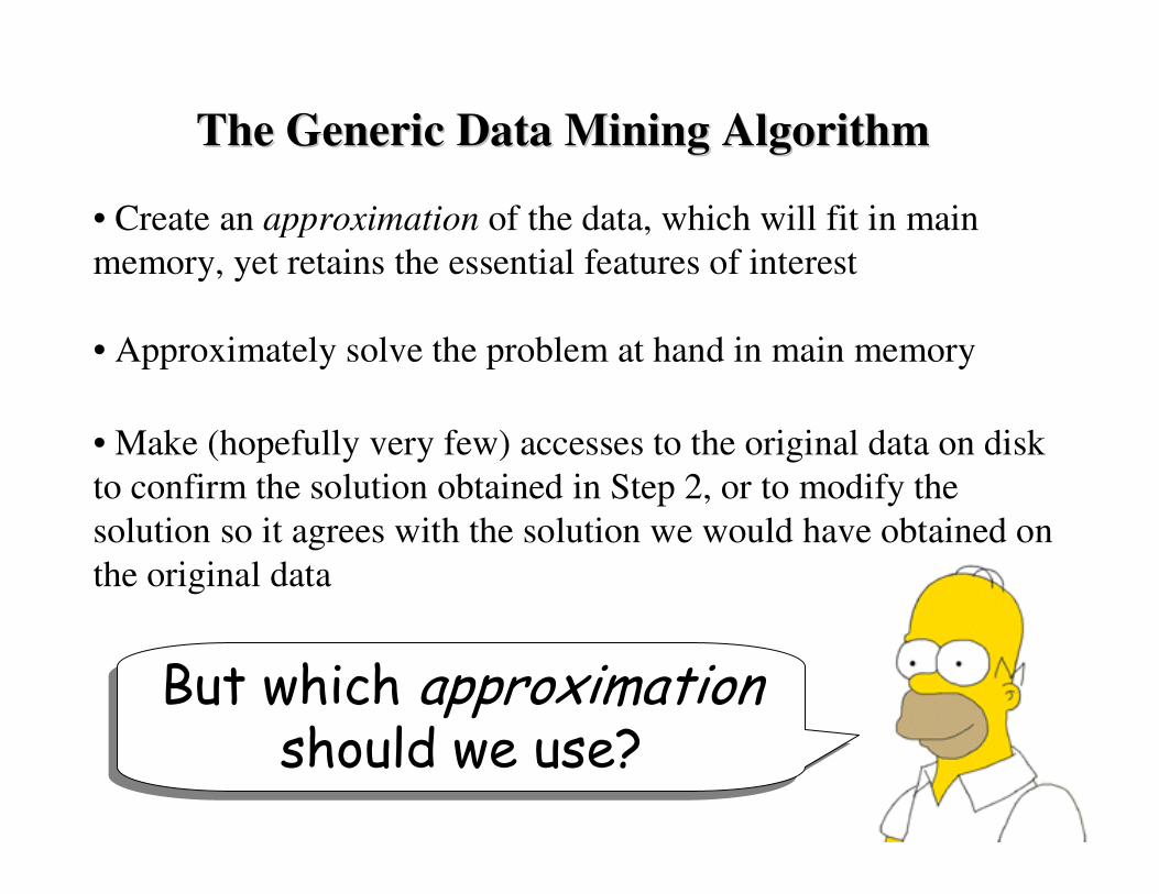
• Create an approximation of the data, which will fit in main

memory, yet retains the essential features of interest

• Approximately solve the problem at hand in main memory

• Make (hopefully very few) accesses to the original data on disk

to confirm the solution obtained in Step 2, or to modify the

solution so it agrees with the solution we would have obtained on

the original data

The Generic Data Mining AlgorithmThe Generic Data Mining Algorithm

But which approximationshould we use?

But which approximationshould we use?

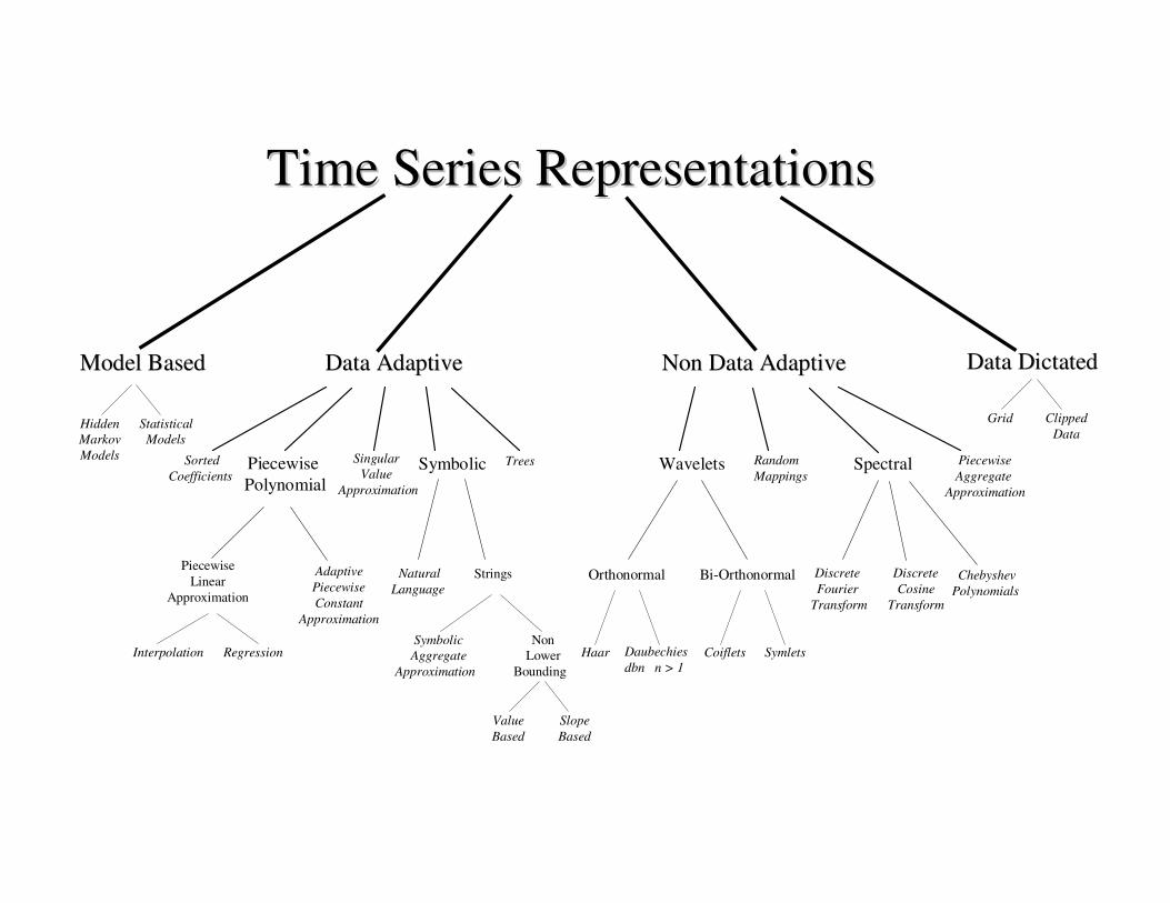
Time Series RepresentationsTime Series Representations

Data AdaptiveData Adaptive Non Data AdaptiveNon Data Adaptive

SpectralWavelets Piecewise

Aggregate

Approximation

Piecewise

Polynomial

SymbolicSingular

Value

Approximation

Random

Mappings

Piecewise

Linear

Approximation

Adaptive

Piecewise

Constant

Approximation

Discrete

Fourier

Transform

Discrete

Cosine

Transform

Haar Daubechies

dbn n > 1

Coiflets Symlets

Sorted

Coefficients

Orthonormal Bi-Orthonormal

Interpolation Regression

Trees

Natural

Language

Strings

Symbolic

Aggregate

Approximation

Non

Lower

Bounding

Chebyshev

Polynomials

Data DictatedData DictatedModel BasedModel Based

Hidden

Markov

Models

Statistical

Models

Value

Based

Slope

Based

Grid Clipped

Data

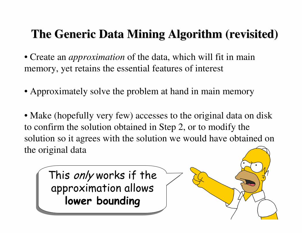
• Create an approximation of the data, which will fit in main

memory, yet retains the essential features of interest

• Approximately solve the problem at hand in main memory

• Make (hopefully very few) accesses to the original data on disk

to confirm the solution obtained in Step 2, or to modify the

solution so it agrees with the solution we would have obtained on

the original data

The Generic Data Mining Algorithm (revisited) The Generic Data Mining Algorithm (revisited)

This only works if the approximation allows

lower bounding

This only works if the approximation allows

lower bounding

Lets take a tour of other time series problemsLets take a tour of other time series problems

• Before we do, let us briefly

revisit SAX, since it has some

implications for the other

problems…

• One central theme of this tutorial is that lowerbounding is

a very useful property. (recall the lower bounds of DTW /uniform scaling, also

recall the importance of lower bounding dimensionality reduction techniques).

•Another central theme is that dimensionality reduction is

very important. That’s why we spend so long discussing

DFT, DWT, SVD, PAA etc.

• Until last year there was no lowerbounding,

dimensionality reducing representation of time series. In

the next slide, let us think about what it means to have

such a representation…

Exploiting Symbolic Representations of Time SeriesExploiting Symbolic Representations of Time Series

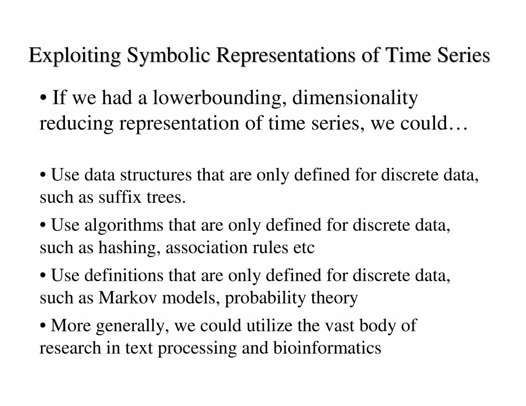
• If we had a lowerbounding, dimensionality

reducing representation of time series, we could…

• Use data structures that are only defined for discrete data,

such as suffix trees.

• Use algorithms that are only defined for discrete data,

such as hashing, association rules etc

• Use definitions that are only defined for discrete data,

such as Markov models, probability theory

• More generally, we could utilize the vast body of

research in text processing and bioinformatics



-3

-2 -1 0 1 2 3

DFT

PLA

Haar

APCA

a b c d e f

SAX

SAX

There is now a lower bounding dimensionality

reducing time series representation! It is called

SAX (Symbolic Aggregate ApproXimation)

I expect SAX to have a major impact on time

series data mining in the coming years…

ffffffeeeddcbaabceedcbaaaaacddee

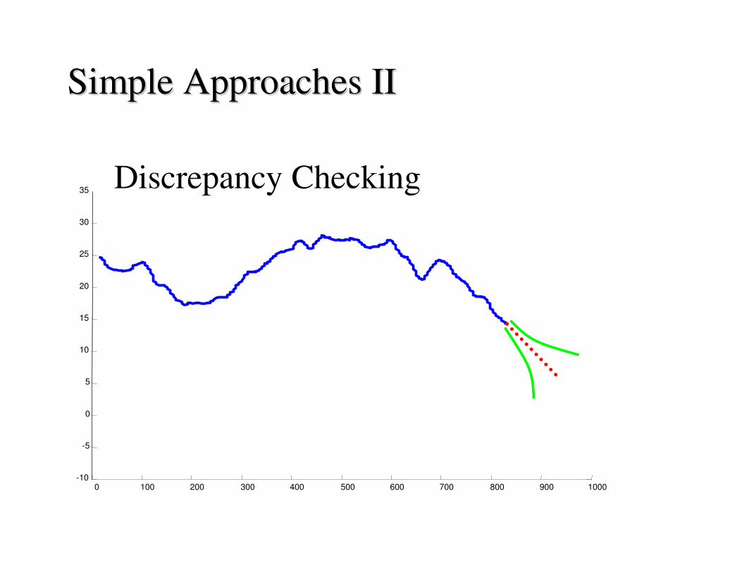
Anomaly (interestingness) detectionAnomaly (interestingness) detection

We would like to be able to discover surprising (unusual, interesting,

anomalous) patterns in time series.

Note that we don’t know in advance in what way the time series

might be surprising

Also note that “surprising” is very context dependent, application

dependent, subjective etc.

0 100 200 300 400 500 600 700 800 900 1000-10

-5

0

5

10

15

20

25

30

35Limit Checking

Simple Approaches ISimple Approaches I

0 100 200 300 400 500 600 700 800 900 1000-10

-5

0

5

10

15

20

25

30

35Discrepancy Checking

Simple Approaches IISimple Approaches II

Early statistical

detection of anthrax

outbreaks by tracking

over-the-counter

medication sales

Goldenberg, Shmueli,

Caruana, and Fienberg

Discrepancy Checking: ExampleDiscrepancy Checking: Example

normalized sales

de-noised

threshold

Actual value

Predicted value

The actual value is

greater than the predicted

value, but still less than

the threshold, so no alarm

is sounded.

• Note that this problem has been solved for text strings

• You take a set of text which has been labeled

“normal”, you learn a Markov model for it.

• Then, any future data that is not modeled well by the

Markov model you annotate as surprising.

• Since we have just seen that we can convert time

series to text (i.e SAX). Lets us quickly see if we can

use Markov models to find surprises in time series…

0 2000 4000 6000 8000 10000 12000

0 2000 4000 6000 8000 10000 12000

0 2000 4000 6000 8000 10000 12000

Training

data

Test data

(subset)

Markov model

surprise

These were

converted to the

symbolic

representation.

I am showing the

original data for

simplicity

0 2000 4000 6000 8000 10000 12000

0 2000 4000 6000 8000 10000 12000

0 2000 4000 6000 8000 10000 12000

Training

data

Test data

(subset)

Markov model

surprise

In the next slide we will zoom in on In the next slide we will zoom in on

this subsection, to try to understand this subsection, to try to understand

why it is surprisingwhy it is surprising

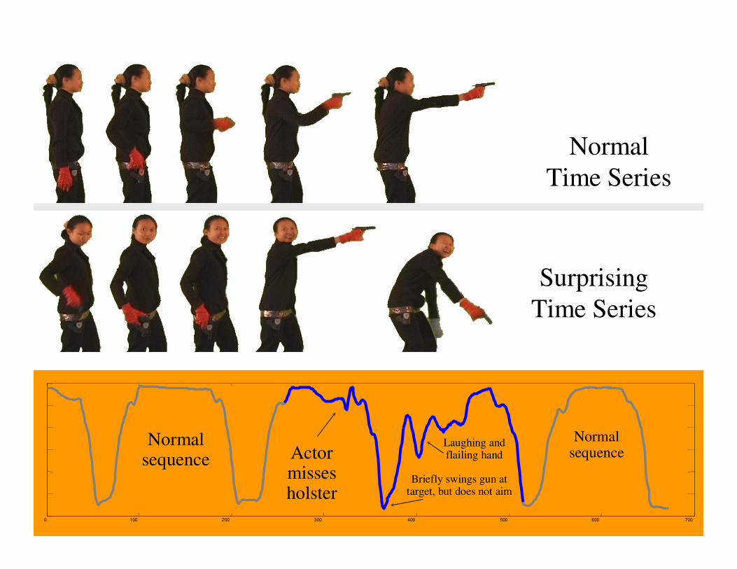
0 100 200 300 400 500 600 700

Normal sequence

Normal sequenceActor

misses holster

Briefly swings gun at target, but does not aim

Laughing and flailing hand

Normal

Time Series

Surprising

Time Series

Anomaly (interestingness) detectionAnomaly (interestingness) detection

In spite of the nice example in the previous slide, the

anomaly detection problem is wide open.

How can we find interesting patterns…

• Without (or with very few) false positives…

• In truly massive datasets...

• In the face of concept drift…

• With human input/feedback…

• With annotated data…

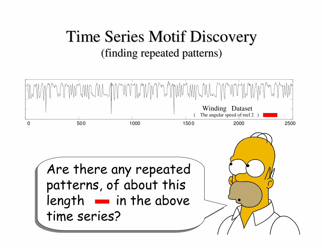
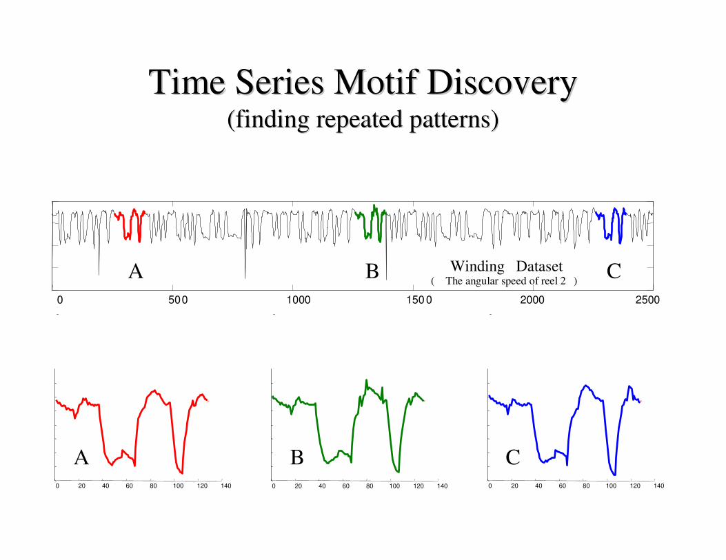
Time Series Motif Discovery Time Series Motif Discovery (finding repeated patterns)(finding repeated patterns)

Winding Dataset( The angular speed of reel 2 )

0 500 1000 150 0 2000 2500

Are there any repeated patterns, of about this length in the above time series?

Are there any repeated patterns, of about this length in the above time series?


0 500 1000 150 0 2000 2500

0 20 40 60 80 100 120 140 0 20 40 60 80 100 120 140 0 20 40 60 80 100 120 140

A B C

A B C

Time Series Motif Discovery Time Series Motif Discovery (finding repeated patterns)(finding repeated patterns)

· Mining association rules in time series requires the discovery of motifs.

These are referred to as primitive shapes and frequent patterns.

· Several time series classification algorithms work by constructing typical

prototypes of each class. These prototypes may be considered motifs.

· Many time series anomaly/interestingness detection algorithms essentially

consist of modeling normal behavior with a set of typical shapes (which we see

as motifs), and detecting future patterns that are dissimilar to all typical shapes.

· In robotics, Oates et al., have introduced a method to allow an autonomous

agent to generalize from a set of qualitatively different experiences gleaned

from sensors. We see these “experiences” as motifs.

· In medical data mining, Caraca-Valente and Lopez-Chavarrias have

introduced a method for characterizing a physiotherapy patient’s recovery

based of the discovery of similar patterns. Once again, we see these “similar

patterns” as motifs.

• Animation and video capture… (Tanaka and Uehara, Zordan and Celly)

Why Find Motifs?Why Find Motifs?

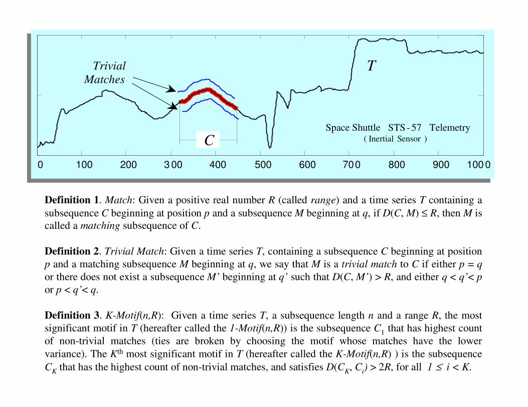
Definition 1. Match: Given a positive real number R (called range) and a time series T containing a

subsequence C beginning at position p and a subsequence M beginning at q, if D(C, M) ≤ R, then M is

called a matching subsequence of C.

Definition 2. Trivial Match: Given a time series T, containing a subsequence C beginning at position

p and a matching subsequence M beginning at q, we say that M is a trivial match to C if either p = q

or there does not exist a subsequence M’ beginning at q’ such that D(C, M’) > R, and either q < q’< p

or p < q’< q.

Definition 3. K-Motif(n,R): Given a time series T, a subsequence length n and a range R, the most

significant motif in T (hereafter called the 1-Motif(n,R)) is the subsequence C1

that has highest count

of non-trivial matches (ties are broken by choosing the motif whose matches have the lower

variance). The Kth most significant motif in T (hereafter called the K-Motif(n,R) ) is the subsequence

CK

that has the highest count of non-trivial matches, and satisfies D(CK, C

i) > 2R, for all 1 ≤ i < K.

0 100 200 3 00 400 500 600 700 800 900 100 0

T

Space Shuttle STS - 57 Telemetry( Inertial Sensor )

Trivial

Matches

C

OK, we can define motifs, but OK, we can define motifs, but

how do we find them?how do we find them?

The obvious brute force search algorithm is just too slow…

The most reference algorithm is based on a hot idea from

bioinformatics, random projection* and the fact that SAX

allows use to lower bound discrete representations of time

series.

* J Buhler and M Tompa. Finding

motifs using random projections. In

RECOMB'01. 2001.

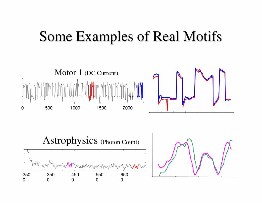
Some Examples of Real MotifsSome Examples of Real Motifs

0 500 1000 1500 2000

Motor 1 (DC Current)

2500

3500

4500

5500

6500

Astrophysics (Photon Count)


0 500 1000 150 0 2000 2500

A B C

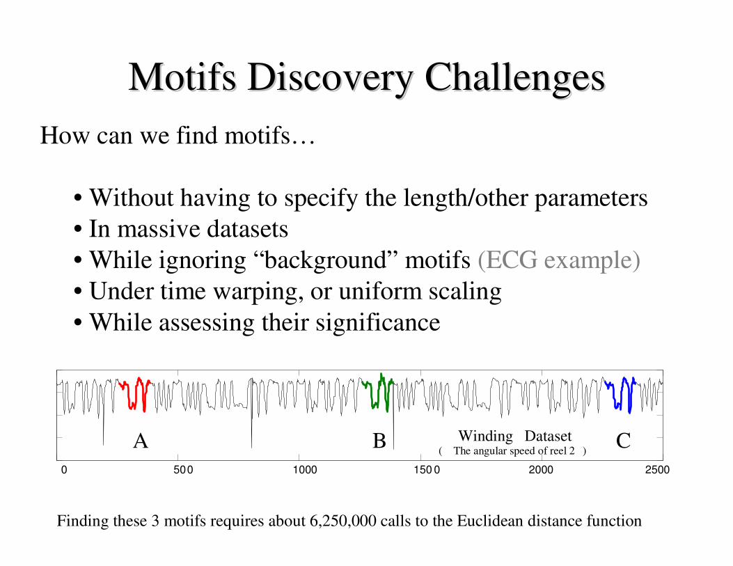
Finding these 3 motifs requires about 6,250,000 calls to the Euclidean distance function

Motifs Discovery Challenges Motifs Discovery Challenges

How can we find motifs…

• Without having to specify the length/other parameters

• In massive datasets

• While ignoring “background” motifs (ECG example)

• Under time warping, or uniform scaling

• While assessing their significance

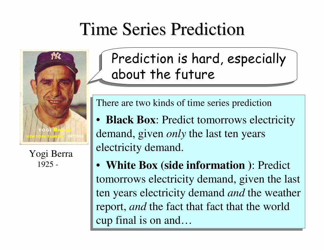
Time Series Prediction Time Series Prediction

There are two kinds of time series prediction

• Black Box: Predict tomorrows electricity

demand, given only the last ten years

electricity demand.

• White Box (side information ): Predict

tomorrows electricity demand, given the last

ten years electricity demand and the weather

report, and the fact that fact that the world

cup final is on and…

There are two kinds of time series prediction

• Black Box: Predict tomorrows electricity

demand, given only the last ten years

electricity demand.

• White Box (side information ): Predict

tomorrows electricity demand, given the last

ten years electricity demand and the weather

report, and the fact that fact that the world

cup final is on and…

Prediction is hard, especially about the future

Prediction is hard, especially about the future

Yogi Berra1925 -

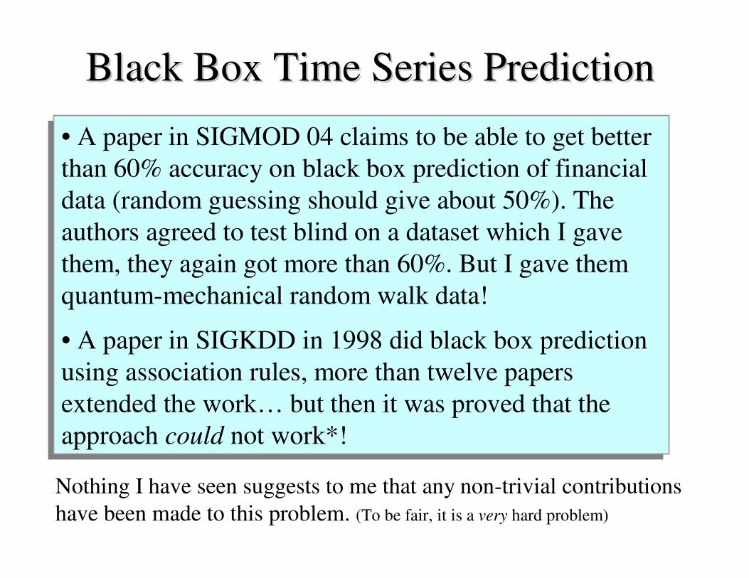
Black Box Time Series Prediction Black Box Time Series Prediction

• A paper in SIGMOD 04 claims to be able to get better

than 60% accuracy on black box prediction of financial

data (random guessing should give about 50%). The

authors agreed to test blind on a dataset which I gave

them, they again got more than 60%. But I gave them

quantum-mechanical random walk data!

• A paper in SIGKDD in 1998 did black box prediction

using association rules, more than twelve papers

extended the work… but then it was proved that the

approach could not work*!

• A paper in SIGMOD 04 claims to be able to get better

than 60% accuracy on black box prediction of financial

data (random guessing should give about 50%). The

authors agreed to test blind on a dataset which I gave

them, they again got more than 60%. But I gave them

quantum-mechanical random walk data!

• A paper in SIGKDD in 1998 did black box prediction

using association rules, more than twelve papers

extended the work… but then it was proved that the

approach could not work*!

Nothing I have seen suggests to me that any non-trivial contributions

have been made to this problem. (To be fair, it is a very hard problem)

introduction to time series mining - didawiki

Documents