introduction to time series analysisjain/cse567-17/ftp/k_37tsa.pdf · 2017-11-07 · what is a time...
TRANSCRIPT

37-1©2017 Raj Jainhttp://www.cse.wustl.edu/~jain/cse567-17/Washington University in St. Louis
Introduction to Introduction to Time Series Time Series
AnalysisAnalysisRaj Jain
Washington University in Saint Louis Saint Louis, MO 63130
[email protected]/Video recordings of this lecture are available at:
http://www.cse.wustl.edu/~jain/cse567-17/
.
37-2©2017 Raj Jainhttp://www.cse.wustl.edu/~jain/cse567-17/Washington University in St. Louis
OverviewOverview
What is a time series?
Autoregressive Models
Moving Average Models
Integrated Models
ARMA, ARIMA, SARIMA, FARIMA models
Note: These slides are based on R. Jain, “The Art of Computer Systems Performance Analysis,”
2nd
Edition (in preparation).

37-3©2017 Raj Jainhttp://www.cse.wustl.edu/~jain/cse567-17/Washington University in St. Louis
Stochastic ProcessesStochastic Processes
Ordered sequence of random observations
Example:
Number of virtual machines in a server
Number of page faults
Number of queries over time
Analysis Technique: Time Series Analysis
Long-range dependence and self-similarity in such processes can invalidate many previous results
37-4©2017 Raj Jainhttp://www.cse.wustl.edu/~jain/cse567-17/Washington University in St. Louis
Stochastic Processes: Key QuestionsStochastic Processes: Key Questions
1.
What is a time series?2.
What are different types of time series models?
3.
How to fit a model to a series of measured data?4.
What is a stationary time series?
5.
Is it possible to model a series that is not stationary?6.
How to model a series that has a periodic or seasonal behavior as is common in video streaming?

37-5©2017 Raj Jainhttp://www.cse.wustl.edu/~jain/cse567-17/Washington University in St. Louis
Stochastic Processes : Key Questions (Cont)Stochastic Processes : Key Questions (Cont)
1.
What are heavy-tailed distributions and why they are important?
2.
How to check if a sample of observations has a heavy tail?
3.
What are self-similar processes?4.
What are short-range and long-range dependent processes?
5.
Why long-range dependence invalidates many conclusions based on previous statistical methods?
6.
How to check if a sample has a long-range dependence?

37-6©2017 Raj Jainhttp://www.cse.wustl.edu/~jain/cse567-17/Washington University in St. Louis
What is a Time SeriesWhat is a Time Series
Time series = Stochastic Process
A sequence of observations over time.
Examples:
Price of a stock over successive days
Sizes of video frames
Sizes of packets over network
Sizes of queries to a database system
Number of active virtual machines in a cloud
Goal: Develop models of such series for resource allocation and improving user experience.
Time t
xt
37-7©2017 Raj Jainhttp://www.cse.wustl.edu/~jain/cse567-17/Washington University in St. Louis
Autoregressive ModelsAutoregressive Models
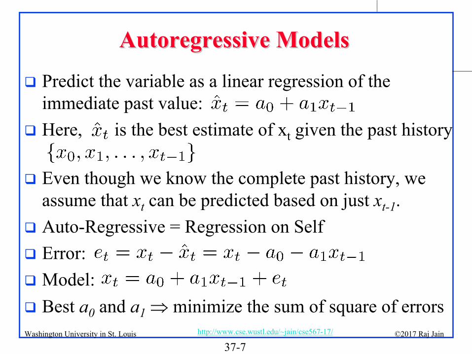
Predict the variable as a linear regression of the immediate past value:
Here, is the best estimate of xt
given the past history
Even though we know the complete past history, we assume that xt
can be predicted based on just xt-1
.
Auto-Regressive = Regression on Self
Error:
Model:
Best a0
and a1
minimize the sum of square of errors
37-8©2017 Raj Jainhttp://www.cse.wustl.edu/~jain/cse567-17/Washington University in St. Louis
Example 37.1Example 37.1
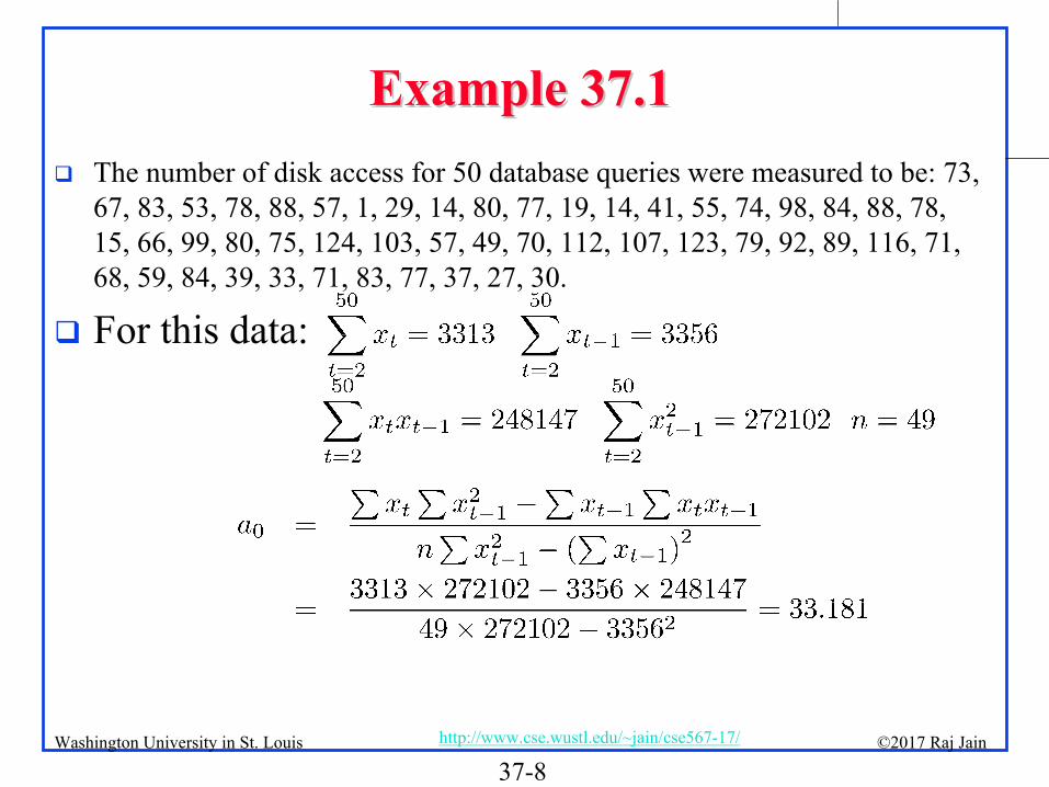
The number of disk access for 50 database queries were measured to be: 73, 67, 83, 53, 78, 88, 57, 1, 29, 14, 80, 77, 19, 14, 41, 55, 74, 98, 84, 88, 78, 15, 66, 99, 80, 75, 124, 103, 57, 49, 70, 112, 107, 123, 79, 92,
89, 116, 71, 68, 59, 84, 39, 33, 71, 83, 77, 37, 27, 30.
For this data:
37-9©2017 Raj Jainhttp://www.cse.wustl.edu/~jain/cse567-17/Washington University in St. Louis
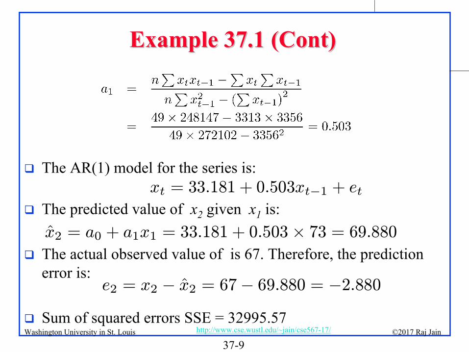
Example 37.1 (Cont)Example 37.1 (Cont)
The AR(1) model for the series is:
The predicted value of x2
given x1
is:
The actual observed value of is 67. Therefore, the prediction error is:
Sum of squared errors SSE = 32995.57
xt = 33.181 + 0.503xt−1 + et
x2 = a0 + a1x1 = 33.181 + 0.503× 73 = 69.880
e2 = x2 − x2 = 67− 69.880 = −2.880

37-10©2017 Raj Jainhttp://www.cse.wustl.edu/~jain/cse567-17/Washington University in St. Louis
Exercise 37.1
Fit an AR(1) model to the following sample of 50 observations: 83, 86, 46, 34, 130, 109, 100, 81, 84, 148, 93, 76, 69, 40, 50, 56, 63, 104, 35, 55, 124, 52, 55, 81, 33, 76, 83, 90, 94, 37, -2, 33, 105, 133, 78, 50, 115, 149, 98, 110, 25, 82, 59, 80, 43, 58, 88, 78, 55, 68. Find a0
, a1
and the minimum SSE.
37-11©2017 Raj Jainhttp://www.cse.wustl.edu/~jain/cse567-17/Washington University in St. Louis
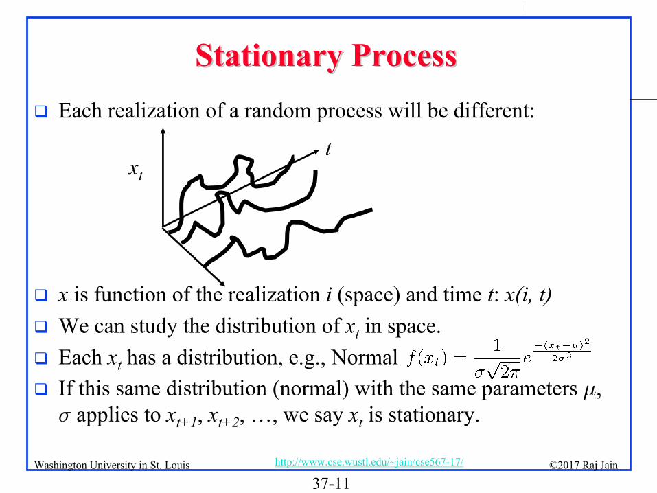
Stationary ProcessStationary Process
Each realization of a random process will be different:
x
is function of the realization i
(space) and time t: x(i, t)
We can study the distribution of xt
in space.
Each xt
has a distribution, e.g., Normal
If this same distribution (normal) with the same parameters μ, σ
applies to xt+1
, xt+2
, …, we say xt
is stationary.
xt
t

37-12©2017 Raj Jainhttp://www.cse.wustl.edu/~jain/cse567-17/Washington University in St. Louis
Stationary Process (Cont)Stationary Process (Cont)
Stationary = Standing in time Distribution does not change with time.
Similarly, the joint distribution of xt
and xt-k
depends only on k not on t.
The joint distribution of xt
, xt-1
, …, xt-k
depends only on k
not on t.
37-13©2017 Raj Jainhttp://www.cse.wustl.edu/~jain/cse567-17/Washington University in St. Louis
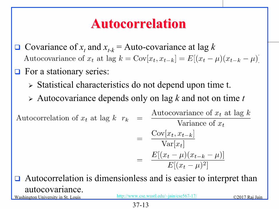
AutocorrelationAutocorrelation
Covariance of xt
and xt-k
= Auto-covariance at lag k
For a stationary series:
Statistical characteristics do not depend upon time t.
Autocovariance
depends only on lag k
and not on time t
Autocorrelation is dimensionless and is easier to interpret than autocovariance.

37-14©2017 Raj Jainhttp://www.cse.wustl.edu/~jain/cse567-17/Washington University in St. Louis
Example 37.2Example 37.2
For the data of Example 37.1, the variance and covariance's at lag 1 and 2 are computed as follows:
50
=1
1 3386Sample Mean = = = 67.7250 50t
tx x
2502 2
=1
1 273002 50 67.72( ) = [( ) ] = ( ) = = 891.87949 49t t t
tVar x E x x x

37-15©2017 Raj Jainhttp://www.cse.wustl.edu/~jain/cse567-17/Washington University in St. Louis
Example 37.2 (Cont)Example 37.2 (Cont)
Small Sample and are slightly different.
Not so for large samples.
Divisor is 48 since we used sample mean calculated from the same sample
1 150
1 1=2
50 50 50 50 50
1 1 1=2 =2 =2 =2 =2
50 50
1=2 =2
50
1=2 =2
( , ) = [( )( )]1= ( )( )48
1 1 1=48 49 49
1 1 4949 49
1 1=48 49
t t t t
t t t tt
t t t t t tt t t t t
t tt t
t tt t
Cov x x E x x
x x x x
x x x x x x
x x
x x
50 50
1=2
1 3313 3356= 248147 = 442.50648 49
t tt
x x
tx 1tx

37-16©2017 Raj Jainhttp://www.cse.wustl.edu/~jain/cse567-17/Washington University in St. Louis
Example 37.2 (Cont)Example 37.2 (Cont)
Note: Only 48 pairs of {xt
, xt-1
} Divisor is 47
2 250
2 2=3
50 50 50
2 2=3 =3 =3
( , ) = [( )( )]1= ( )( )47
1 1=47 48
1 3246 3329= 22936047 48
= 90.136
t t t t
t t t tt
t t t tt t t
Cov x x E x x
x x x x
x x x x

37-17©2017 Raj Jainhttp://www.cse.wustl.edu/~jain/cse567-17/Washington University in St. Louis
Example 37.2 (Cont)Example 37.2 (Cont)
0( ) 891.8790 = = = = 1( ) 891.879
t
t
Var xAutocorrelation at lag rVar x
11
( , ) 442.5061 = = = = 0.496( ) 891.879t t
t
Cov x xAutocorrelation at lag rVar x
22
( , ) 90.1362 = = = = 0.101( ) 891.879t t
t
Cov x xAutocorrelation at lag rVar x
Lag k
Aut
ocor
rela
tion
r k
0 1 2
1.0

37-18©2017 Raj Jainhttp://www.cse.wustl.edu/~jain/cse567-17/Washington University in St. Louis
White NoiseWhite Noise
Errors et
are normal independent and identically distributed (IID) with zero mean and variance σ2
Such IID sequences are called “white noise”
sequences.
Properties:
k0
37-19©2017 Raj Jainhttp://www.cse.wustl.edu/~jain/cse567-17/Washington University in St. Louis
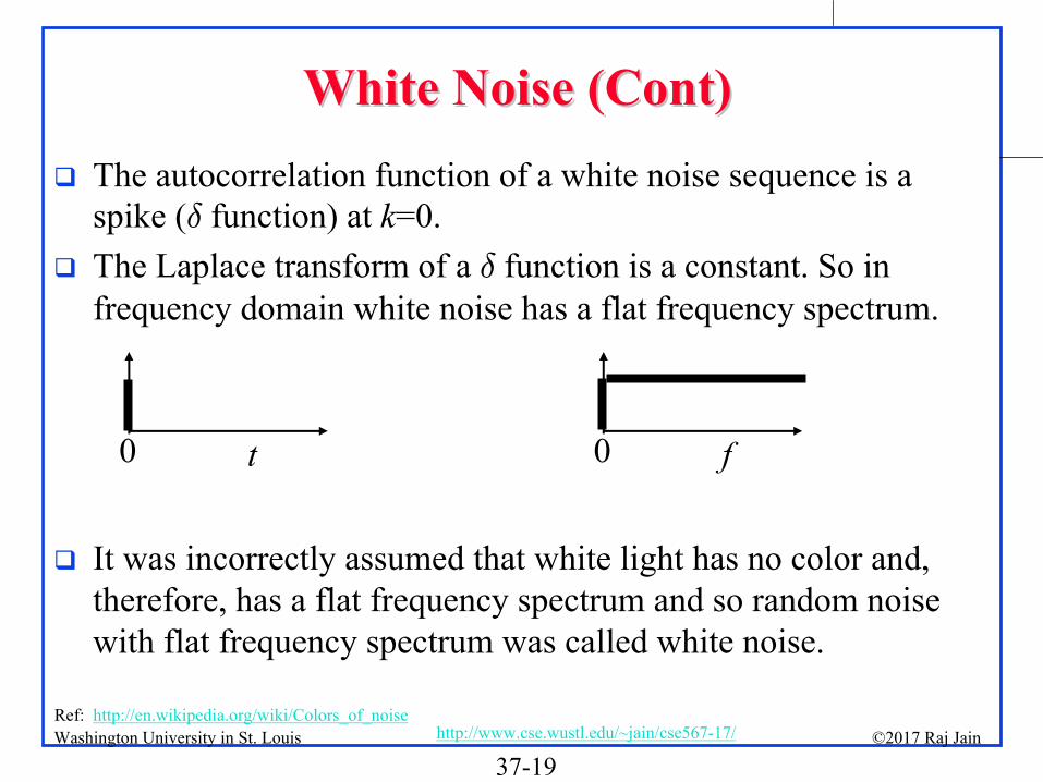
White Noise (Cont)White Noise (Cont)
The autocorrelation function of a white noise sequence is a spike (δ
function) at k=0.
The Laplace transform of a δ
function is a constant. So in frequency domain white noise has a flat frequency spectrum.
It was incorrectly assumed that white light has no color and, therefore, has a flat frequency spectrum and so random noise with flat frequency spectrum was called white noise.
t0 f0
Ref: http://en.wikipedia.org/wiki/Colors_of_noise
37-20©2017 Raj Jainhttp://www.cse.wustl.edu/~jain/cse567-17/Washington University in St. Louis
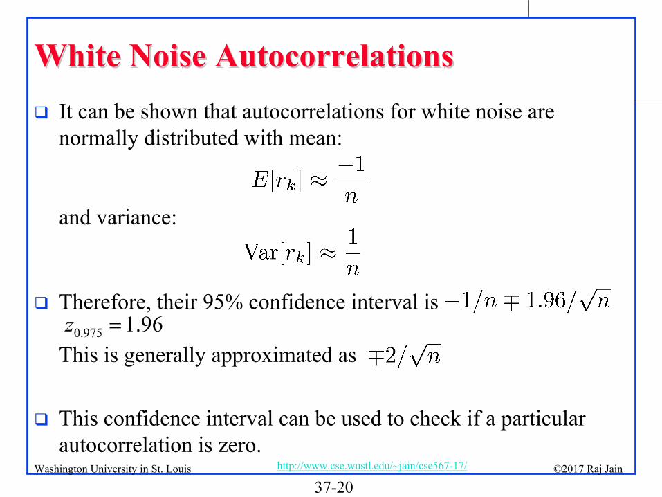
White Noise AutocorrelationsWhite Noise Autocorrelations
It can be shown that autocorrelations for white noise are normally distributed with mean:
and variance:
Therefore, their 95% confidence interval is
This is generally approximated as
This confidence interval can be used to check if a particular autocorrelation is zero.
0.975 1.96z

37-21©2017 Raj Jainhttp://www.cse.wustl.edu/~jain/cse567-17/Washington University in St. Louis
Example 37.3
For the data of Example 37.1: n=50CI = ∓2/
p(50) = ∓0.283
r2
is not significantly different from zero.
37-22©2017 Raj Jainhttp://www.cse.wustl.edu/~jain/cse567-17/Washington University in St. Louis
Exercise 37.2
Determine autocorrelations at lag 0 through 2 for the data of Exercise 37.1 and determine which of these autocorrelations are significant at 95% confidence.
37-23©2017 Raj Jainhttp://www.cse.wustl.edu/~jain/cse567-17/Washington University in St. Louis
Assumptions for AR(1) ModelsAssumptions for AR(1) Models
1.
xt
is a Stationary process 2.
Linear relationship between successive values3.
Normal Independent identically distributed errors:a.
Normal errorsb.
Independent errors4.
Additive errors

37-24©2017 Raj Jainhttp://www.cse.wustl.edu/~jain/cse567-17/Washington University in St. Louis
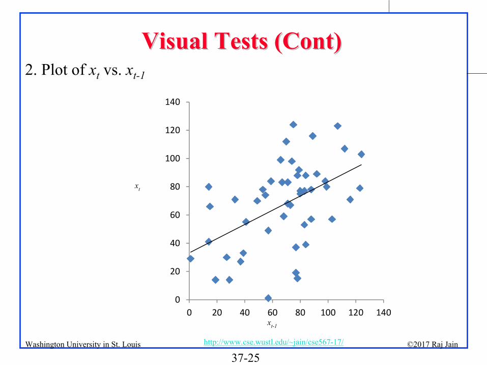
Visual Tests for AR(1) ModelsVisual Tests for AR(1) Models1.
Plot xt
as a function of t
and look for trends2.
xt
vs. xt-1
for linearity3.
Errors et
vs. predicted values for additivity4.
Q-Q Plot of errors for Normality5.
Errors et
vs. t
for IID
1. Plot of xt
37-25©2017 Raj Jainhttp://www.cse.wustl.edu/~jain/cse567-17/Washington University in St. Louis
Visual Tests (Cont)Visual Tests (Cont)2. Plot of
xt
vs. xt-1
0
20
40
60
80
100
120
140
0 20 40 60 80 100 120 140xt-1
xt
37-26©2017 Raj Jainhttp://www.cse.wustl.edu/~jain/cse567-17/Washington University in St. Louis
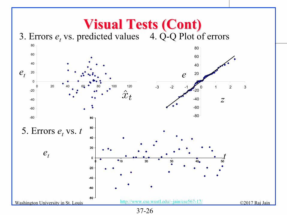
Visual Tests (Cont)Visual Tests (Cont)
-80
-60
-40
-20
0
20
40
60
80
0 20 40 60 80 100 120
et e
z-80
-60
-40
-20
0
20
40
60
80
-3 -2 -1 0 1 2 3
et t
3. Errors et
vs. predicted values 4. Q-Q Plot of errors
5. Errors et
vs. t

37-27©2017 Raj Jainhttp://www.cse.wustl.edu/~jain/cse567-17/Washington University in St. Louis
Exercise 37.3
Conduct visual tests to verify whether or not the AR(1) model fitted in Exercise 37.1 is appropriate .

37-28©2017 Raj Jainhttp://www.cse.wustl.edu/~jain/cse567-17/Washington University in St. Louis
AR(pAR(p) Model) Model
xt
is a function of the last p values:
AR(2):
AR(3):

37-29©2017 Raj Jainhttp://www.cse.wustl.edu/~jain/cse567-17/Washington University in St. Louis
Similarly,
Or
Using this notation, AR(p) model is:
Here, φp
is a polynomial of degree p.
Backward Shift OperatorBackward Shift Operator

37-30©2017 Raj Jainhttp://www.cse.wustl.edu/~jain/cse567-17/Washington University in St. Louis
AR(pAR(p) Parameter Estimation) Parameter Estimation
The coefficients ai
's
can be estimated by minimizing SSE using Multiple Linear Regression.
Optimal a0
, a1
, and a2
Minimize SSE Set the first differential to zero:

37-31©2017 Raj Jainhttp://www.cse.wustl.edu/~jain/cse567-17/Washington University in St. Louis
AR(pAR(p) Parameter Estimation (Cont)) Parameter Estimation (Cont)
The equations can be written as:
Note: All sums are for t=3 to n. n-2
terms.
Multiplying by the inverse of the first matrix, we get:
37-32©2017 Raj Jainhttp://www.cse.wustl.edu/~jain/cse567-17/Washington University in St. Louis
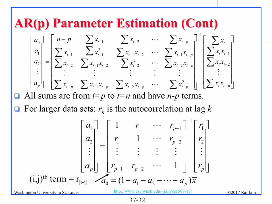
AR(pAR(p) Parameter Estimation (Cont)) Parameter Estimation (Cont)
All sums are from t=p
to t=n
and have n-p
terms.
For larger data sets: rk
is the autocorrelation at lag k
1 1 1 1
2 1 2 2
1
1
2
11
1
p
p
p p p p
a r r ra r r r
a r r r
1 20
21 11 1
1
1 2 12
2 22 1 2 2 2
21 2
t t t p t
t tt t t t t t p
t tt t t t t t p
p t t pt p t t p t t p t p
x x x xx xx x x x xx xx x x x x x
x xx
n paa xa
x x x x xa
0 1 2(1 )pa a a a x (i,j)th
term = r|i-j|
37-33©2017 Raj Jainhttp://www.cse.wustl.edu/~jain/cse567-17/Washington University in St. Louis
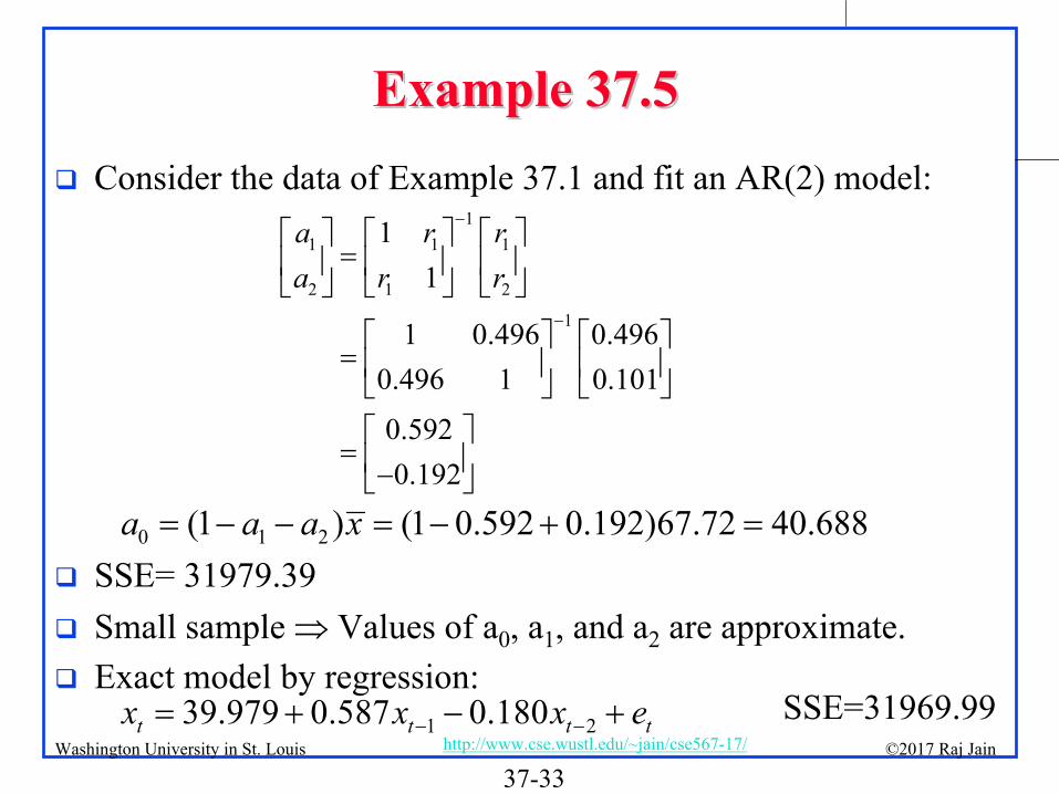
Example 37.5Example 37.5
Consider the data of Example 37.1 and fit an AR(2) model:
SSE= 31979.39
Small sample Values of a0
, a1
, and a2
are approximate.
Exact model by regression:
1 1 1
2 1 2
1
1
11
1 0.496 0.4960.496 1 0.101
0.5920.192
a r ra r r
0 1 2(1 ) (1 0.592 0.192)67.72 40.688a a a x
1 239.979 0.587 0.180t t t tx xx e SSE=31969.99

37-34©2017 Raj Jainhttp://www.cse.wustl.edu/~jain/cse567-17/Washington University in St. Louis
Exercise 37.4
Fit an AR(2) model to the data of Exercise 37.1. Determine parameters a0
, a1
, a2
and the SSE using multiple regression. Repeat the determination of parameters using autocorrelation function values.
37-35©2017 Raj Jainhttp://www.cse.wustl.edu/~jain/cse567-17/Washington University in St. Louis
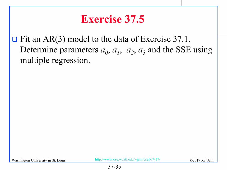
Exercise 37.5
Fit an AR(3) model to the data of Exercise 37.1. Determine parameters a0
, a1
, a2
, a3
and the SSE using multiple regression.
37-36©2017 Raj Jainhttp://www.cse.wustl.edu/~jain/cse567-17/Washington University in St. Louis
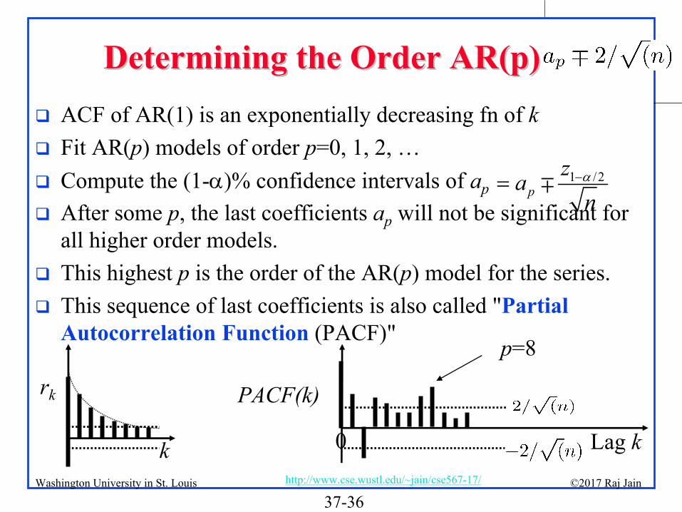
Determining the Order Determining the Order AR(pAR(p))
ACF of AR(1) is an exponentially decreasing fn of k
Fit AR(p) models of order p=0, 1, 2, …
Compute the (1-)% confidence intervals of ap
After some p, the last coefficients ap
will not be significant for all higher order models.
This highest p
is the order of the AR(p) model for the series.
This sequence of last coefficients is also called "Partial Autocorrelation Function
(PACF)"
Lag k
PACF(k)
0
p=8
rk
k
1 /2p
zn
a
37-37©2017 Raj Jainhttp://www.cse.wustl.edu/~jain/cse567-17/Washington University in St. Louis
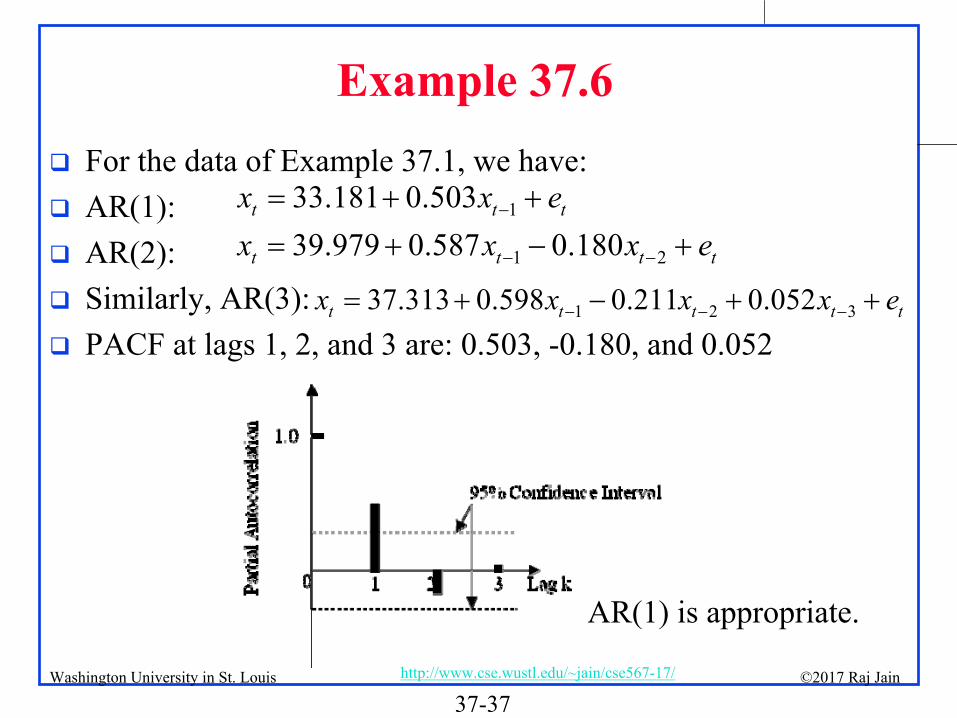
Example 37.6
For the data of Example 37.1, we have:
AR(1):
AR(2):
Similarly, AR(3):
PACF at lags 1, 2, and 3 are: 0.503, -0.180, and 0.052
133.181 0.503t t tx x e
1 239.979 0.587 0.180t t t tx x x e
1 2 337.313 0.598 0.211 0.052t t t t tx x x x e
AR(1) is appropriate.

37-38©2017 Raj Jainhttp://www.cse.wustl.edu/~jain/cse567-17/Washington University in St. Louis
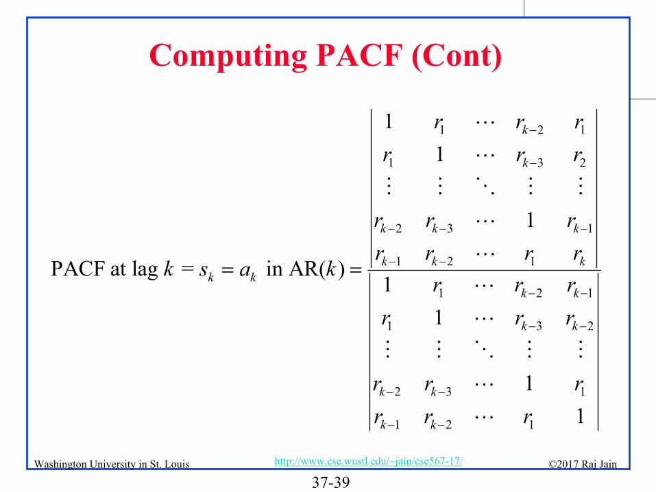
Computing PACF
1 1 1
1
1 22
1
1
1 1
1 2
2 1 33 3
1 2
1 1
2 1
2
in AR(1)
in
PACF at lag 1 = s 1
PACF at lag 2 = s 1
1
11
PACF at lag 3 = s 1
AR(2)
in AR(3)
11
rr r
rr
r rr rr r r
r rr r
a r
r
a
a
r
M = Determinant of M
37-39©2017 Raj Jainhttp://www.cse.wustl.edu/~jain/cse567-17/Washington University in St. Louis
Computing PACF (Cont)
1 2 1
1 3 2
2 3 1
1 2 1
1 2 1
1 3 2
2 3 1
1 2 1
11
in AR( )
1
PACF at lag =1
1
1
1
k
k
k k k
k k kk
k k
k k
k k
k k
k
r r rr r r
r r rr r r r
a kr r r
r r r
r r rr r
k s
r
37-40©2017 Raj Jainhttp://www.cse.wustl.edu/~jain/cse567-17/Washington University in St. Louis
Exercise 37.6
Using the results of Exercises 37.1, 37.4, and 37.5, determine the partial autocorrelation function at lags 1, 2, 3 for the data of Exercise 37.1. Determine which values are significant. Based on this which AR(p) model will be appropriate for this data?
37-41©2017 Raj Jainhttp://www.cse.wustl.edu/~jain/cse567-17/Washington University in St. Louis
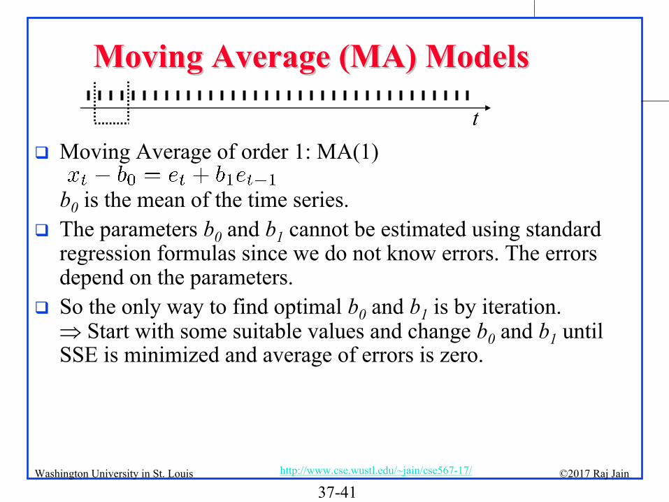
Moving Average (MA) ModelsMoving Average (MA) Models
Moving Average of order 1: MA(1) b0
is the mean of the time series.
The parameters b0
and b1
cannot be estimated using standard regression formulas since we do not know errors. The errors depend on the parameters.
So the only way to find optimal b0
and b1
is by iteration. Start with some suitable values and change b0
and b1
until SSE is minimized and average of errors is zero.
t
37-42©2017 Raj Jainhttp://www.cse.wustl.edu/~jain/cse567-17/Washington University in St. Louis
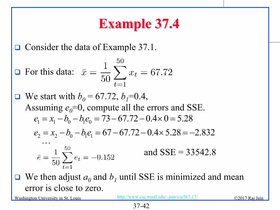
Example 37.4Example 37.4
Consider the data of Example 37.1.
For this data:
We start with b0
= 67.72, b1
=0.4, Assuming e0
=0, compute all the errors and SSE.
and SSE = 33542.8
We then adjust a0
and b1
until SSE is minimized and mean error is close to zero.
1 1 0 1 0 73 67.72 0.4 0 5.28e x b b e
2 2 0 1 1 67 67.72 0.4 5.28 2.832e x b b e …

37-43©2017 Raj Jainhttp://www.cse.wustl.edu/~jain/cse567-17/Washington University in St. Louis
Example 37.4 (Cont)Example 37.4 (Cont)
The steps are: Starting with and trying various values of b1
. SSE is minimum at b1
=0.475. SSE= 33221.06

37-44©2017 Raj Jainhttp://www.cse.wustl.edu/~jain/cse567-17/Washington University in St. Louis
Example 37.4 (Cont)Example 37.4 (Cont)
Keeping b1
=0.475, try neighboring values of b0
to get average error as close to zero as possible.
b0
= 67.475 gives =-0.001 SSE=33221.93
50
=1
1= = 0.166150 t
te e
e
37-45©2017 Raj Jainhttp://www.cse.wustl.edu/~jain/cse567-17/Washington University in St. Louis
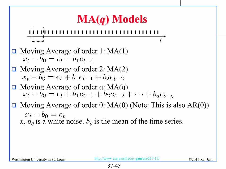
MA(MA(qq) Models) Models
Moving Average of order 1: MA(1)
Moving Average of order 2: MA(2)
Moving Average of order q: MA(q)
Moving Average of order 0: MA(0) (Note: This is also AR(0)) xt
-b0
is a white noise. b0
is the mean of the time series.
t
37-46©2017 Raj Jainhttp://www.cse.wustl.edu/~jain/cse567-17/Washington University in St. Louis
Exercise 37.7
Fit an MA(0) model to the data of Exercise 37.1. Determine parameter b0
and SSE

37-47©2017 Raj Jainhttp://www.cse.wustl.edu/~jain/cse567-17/Washington University in St. Louis
MA(qMA(q) Models (Cont)) Models (Cont)
Using the backward shift operator B, MA(q):
Here, Ψq
is a polynomial of order q.

37-48©2017 Raj Jainhttp://www.cse.wustl.edu/~jain/cse567-17/Washington University in St. Louis
Example 37.8
Fit MA(2) model to the data of Example 37.1
Round 1: Setting , we try 9 combinations of b1
={0.2,0.3,0.4} and b2
={0.2, 0.3, 0.4}. Minimum SSE is 33490.26 at b1
=0.4 and b2
=0.2
Round 2: Try 4 new points around the current minimum b0
={0.35, 0.45} and b2
={0.15, 0.25} Minimum SSE is 32551.62 at b1
=0.45, b2
=0.15
Round 3: Try 4 new points around the current minimum. Try b1
={0.425, 0.475} and b2
={0.125, 0.175} Minimum SSE is 32342.61 at b1
=0.475, b2
=0.125
0 1 1 2 2t t t tx b e b e b e
b0 = xt = 67.72
37-49©2017 Raj Jainhttp://www.cse.wustl.edu/~jain/cse567-17/Washington University in St. Louis
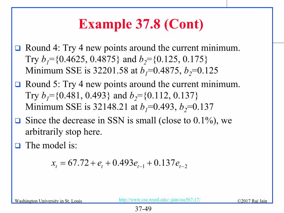
Example 37.8 (Cont)
Round 4: Try 4 new points around the current minimum. Try b1
={0.4625, 0.4875} and b2
={0.125, 0.175} Minimum SSE is 32201.58 at b1
=0.4875, b2
=0.125
Round 5: Try 4 new points around the current minimum. Try b1
={0.481, 0.493} and b2
={0.112, 0.137} Minimum SSE is 32148.21 at b1
=0.493, b2
=0.137
Since the decrease in SSN is small (close to 0.1%), we arbitrarily stop here.
The model is:
1 267.72 0.493 0.137t t t tx e e e

37-50©2017 Raj Jainhttp://www.cse.wustl.edu/~jain/cse567-17/Washington University in St. Louis
Exercise 38.8
Fit an MA(1) model to the data of Exercise 37.1. Determine parameters b0
, b1
and the minimum SSE.
37-51©2017 Raj Jainhttp://www.cse.wustl.edu/~jain/cse567-17/Washington University in St. Louis
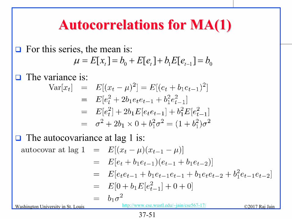
Autocorrelations for MA(1)Autocorrelations for MA(1)
For this series, the mean is:
The variance is:
The autocovariance
at lag 1 is:
0 1 1 0[ ] [ ] [ ]t t tE x b E e b E e b
37-52©2017 Raj Jainhttp://www.cse.wustl.edu/~jain/cse567-17/Washington University in St. Louis
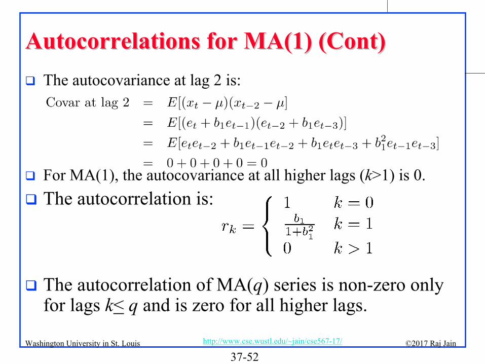
Autocorrelations for MA(1) (Cont)Autocorrelations for MA(1) (Cont)
The autocovariance
at lag 2 is:
For MA(1), the autocovariance
at all higher lags (k>1) is 0.
The autocorrelation is:
The autocorrelation of MA(q) series is non-zero only for lags k<
q and is zero for all higher lags.

37-53©2017 Raj Jainhttp://www.cse.wustl.edu/~jain/cse567-17/Washington University in St. Louis
Example 37.9
For the data of Example 37.1:
Autocorrelation is zero for all lags k >1.
MA(1) model is appropriate for this data.

37-54©2017 Raj Jainhttp://www.cse.wustl.edu/~jain/cse567-17/Washington University in St. Louis
Example 37.10Example 37.10
The order of the last significant rk
determines the order of the MA(q) model.
For the following data, all autocorrelations at lag 9 and higher are zero MA(8) model would be appropriate
Lag k
Autocorrelation rk
0
q=8

37-55©2017 Raj Jainhttp://www.cse.wustl.edu/~jain/cse567-17/Washington University in St. Louis
Exercise 37.9
Fit an MA(2) model to the data of Exercise 37.2. Determine parameters b0
, b1
, b2
and the minimum SSE. For this data, which model would you choose MA(0), MA(1) or MA(2) and why?

37-56©2017 Raj Jainhttp://www.cse.wustl.edu/~jain/cse567-17/Washington University in St. Louis
Duality of AR(p) vs. MA(q)
Determining the coefficients of AR(p) is straight forward but determining the order p requires an iterative procedure
Determining the order q of MA(q) is straight forward but determining the coefficients requires an iterative procedure
37-57©2017 Raj Jainhttp://www.cse.wustl.edu/~jain/cse567-17/Washington University in St. Louis
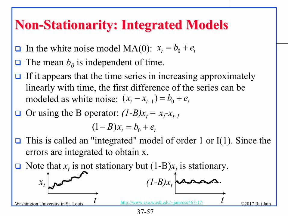
NonNon--StationarityStationarity: Integrated Models: Integrated Models
In the white noise model MA(0):
The mean b0
is independent of time.
If it appears that the time series in increasing approximately linearly with time, the first difference of the series can be modeled as white noise:
Or using the B operator: (1-B)xt
= xt
-xt-1
This is called an "integrated" model of order 1 or I(1). Since the errors are integrated to obtain x.
Note that xt
is not stationary but (1-B)xt
is stationary.
t
xt
t
(1-B)xt
0t tx b e
1 0)( t t tx x b e
0(1 ) t tB x b e
37-58©2017 Raj Jainhttp://www.cse.wustl.edu/~jain/cse567-17/Washington University in St. Louis
Integrated Models (Cont)Integrated Models (Cont)
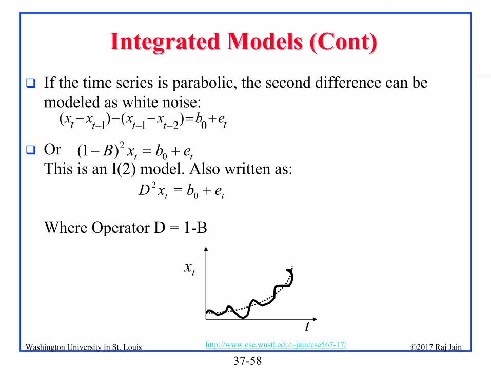
If the time series is parabolic, the second difference can be modeled as white noise:
Or This is an I(2) model. Also written as:
Where Operator D = 1-B
t
xt
20=t tD x b e
1 1 2 0) (( )t tt t txx x x b e
20(1 ) t txB b e

37-59©2017 Raj Jainhttp://www.cse.wustl.edu/~jain/cse567-17/Washington University in St. Louis
ARMA and ARIMA ModelsARMA and ARIMA Models
It is possible to combine AR, MA, and I models
ARMA(p, q) Model:
ARIMA(p,d,q) Model:
Using algebraic manipulations, it is possible to transform AR models to MA models and vice versa.

37-60©2017 Raj Jainhttp://www.cse.wustl.edu/~jain/cse567-17/Washington University in St. Louis
Example 37.11
Consider the MA(1) model:
It can be written as:0 1 1t t tx b e b e
0 1( ) (1 )t tx b b B e
11 0(1 ) ( )t tb B x b e
2 2 3 31 1 1 01 ... ( )t tb B b B b B x b e
2 3 01 1 1 2 1 3
11t t t t tbx b x b x b x e
b
2 301 1 1 2 1 3
11t t t t tbx b x b x b x e
b
If b1
<1, the coefficients decrease and soon become insignificant. This results in a finite order AR model.

37-61©2017 Raj Jainhttp://www.cse.wustl.edu/~jain/cse567-17/Washington University in St. Louis
Exercise 39.10
Convert the following AR(1) model to an equivalent MA model:
0 1 1t t tx a a x e
37-62©2017 Raj Jainhttp://www.cse.wustl.edu/~jain/cse567-17/Washington University in St. Louis
NonNon--StationarityStationarity
due to Seasonalitydue to Seasonality
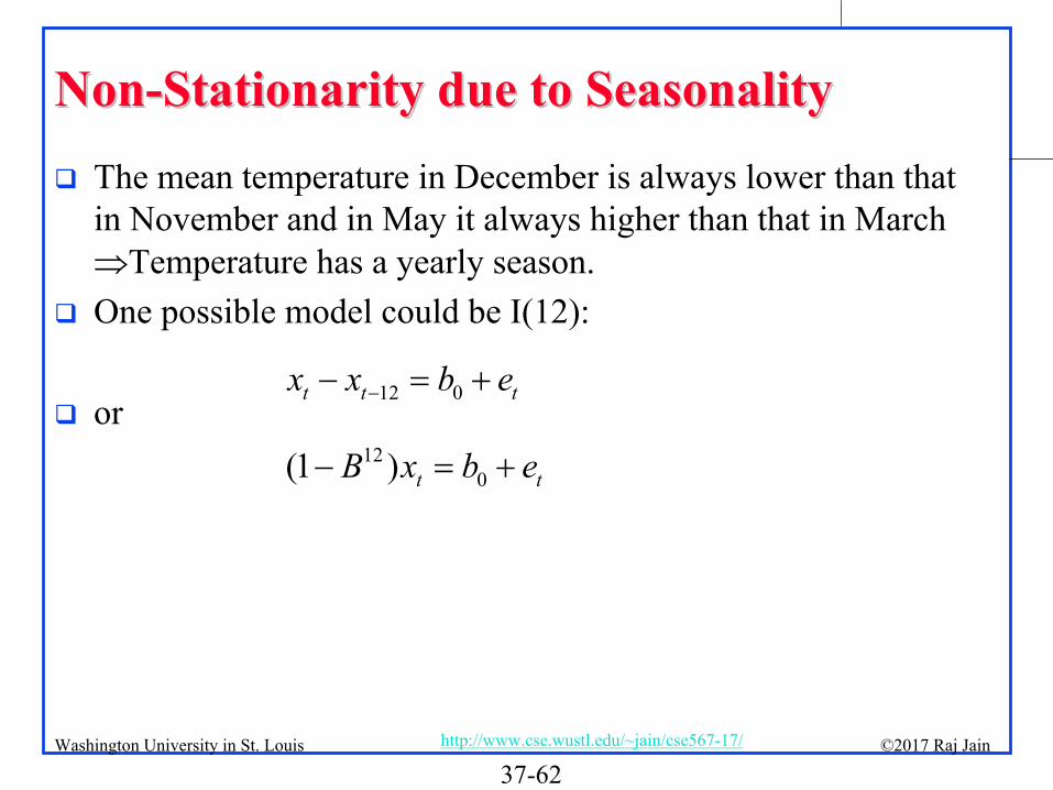
The mean temperature in December is always lower than that in November and in May it always higher than that in March Temperature has a yearly season.
One possible model could be I(12):
or12 0t t tx x b e
120)(1 t tx b eB
37-63©2017 Raj Jainhttp://www.cse.wustl.edu/~jain/cse567-17/Washington University in St. Louis
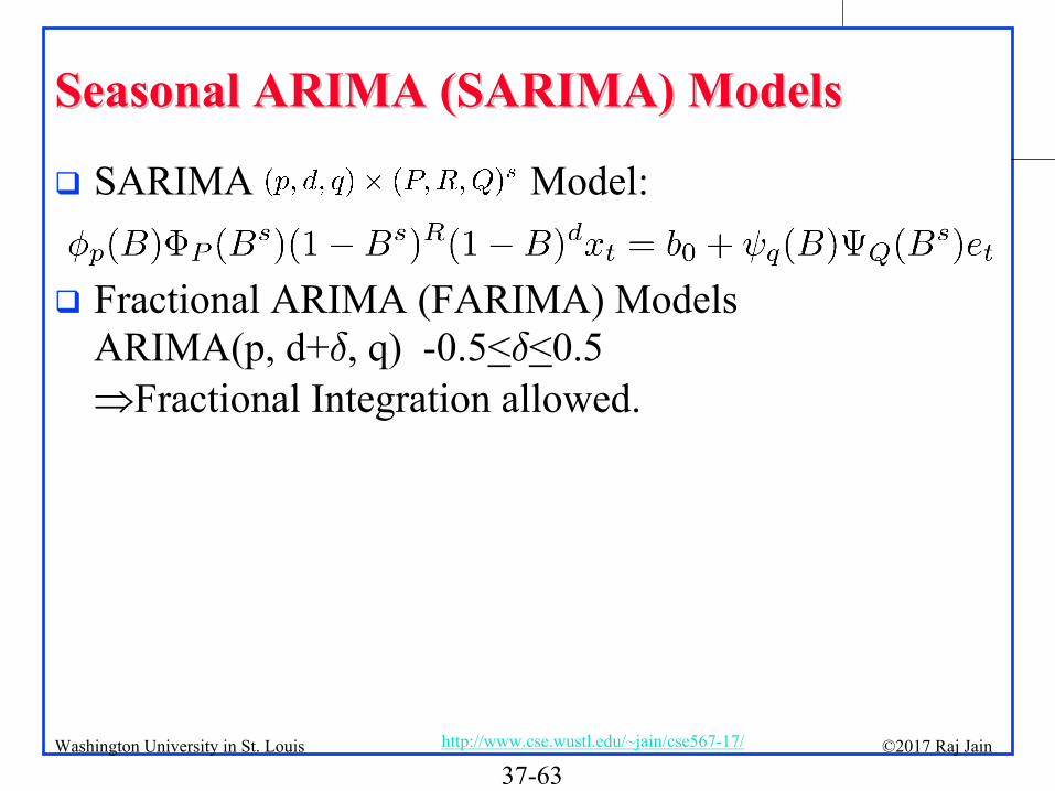
Seasonal ARIMA (SARIMA) ModelsSeasonal ARIMA (SARIMA) Models
SARIMA Model:
Fractional ARIMA (FARIMA) Models ARIMA(p, d+δ, q) -0.5<δ<0.5
Fractional Integration allowed.
37-64©2017 Raj Jainhttp://www.cse.wustl.edu/~jain/cse567-17/Washington University in St. Louis
Exercise 37.11
Write the expression for SARIMA(1,0,1)(0,1,0)12
model in terms of x’s
and e’s.
37-65©2017 Raj Jainhttp://www.cse.wustl.edu/~jain/cse567-17/Washington University in St. Louis
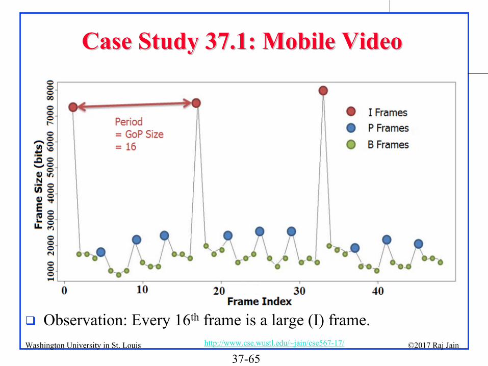
Observation: Every 16th
frame is a large (I) frame.
Case Study 37.1: Mobile VideoCase Study 37.1: Mobile Video

37-66©2017 Raj Jainhttp://www.cse.wustl.edu/~jain/cse567-17/Washington University in St. Louis
A closer look at the ACF graph shows a strong continual correlation every 16 lag GOP size
Traffic Modeling Traffic Modeling ––
All FramesAll Frames
Result: SARIMA (1, 0, 1)x(1,1,1)s
Model, s=group size =16

37-67©2017 Raj Jainhttp://www.cse.wustl.edu/~jain/cse567-17/Washington University in St. Louis
Validation
37-68©2017 Raj Jainhttp://www.cse.wustl.edu/~jain/cse567-17/Washington University in St. Louis
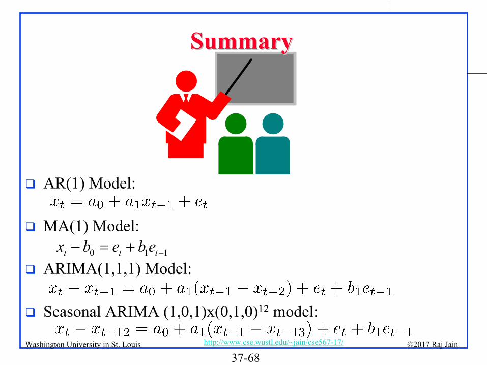
SummarySummary
AR(1) Model:
MA(1) Model:
ARIMA(1,1,1) Model:
Seasonal ARIMA (1,0,1)x(0,1,0)12
model:
0 1 1t t tbx e b e

37-69©2017 Raj Jainhttp://www.cse.wustl.edu/~jain/cse567-17/Washington University in St. Louis
Scan This to Download These Slides
Raj Jainhttp://rajjain.com

37-70©2017 Raj Jainhttp://www.cse.wustl.edu/~jain/cse567-17/Washington University in St. Louis
Related Modules
Video Podcasts of Prof. Raj Jain's Lectures, https://www.youtube.com/channel/UCN4-5wzNP9-ruOzQMs-8NUw
CSE473S: Introduction to Computer Networks (Fall 2011), https://www.youtube.com/playlist?list=PLjGG94etKypJWOSPMh8Azcgy5e_10TiDw
Wireless and Mobile Networking (Spring 2016), https://www.youtube.com/playlist?list=PLjGG94etKypKeb0nzyN9tSs_HCd5c4wXF
CSE567M: Computer Systems Analysis (Spring 2013), https://www.youtube.com/playlist?list=PLjGG94etKypJEKjNAa1n_1X0bWWNyZcof
CSE571S: Network Security (Fall 2011), https://www.youtube.com/playlist?list=PLjGG94etKypKvzfVtutHcPFJXumyyg93u