INTRODUCTION TO

Batteries & Fuel Cells Module

C o n t a c t I n f o r m a t i o nVisit the Contact COMSOL page at www.comsol.com/contact to submit general inquiries, contact

Technical Support, or search for an address and phone number. You can also visit the Worldwide

Sales Offices page at www.comsol.com/contact/offices for address and contact information.

If you need to contact Support, an online request form is located at the COMSOL Access page at

www.comsol.com/support/case. Other useful links include:

• Support Center: www.comsol.com/support

• Product Download: www.comsol.com/product-download

• Product Updates: www.comsol.com/support/updates

• COMSOL Blog: www.comsol.com/blogs

• Discussion Forum: www.comsol.com/community

• Events: www.comsol.com/events

• COMSOL Video Gallery: www.comsol.com/video

• Support Knowledge Base: www.comsol.com/support/knowledgebase

Part number: CM021502

I n t r o d u c t i o n t o t h e B a t t e r i e s & F u e l C e l l s M o d u l e © 1998–2018 COMSOL

Protected by patents listed on www.comsol.com/patents, and U.S. Patents 7,519,518; 7,596,474; 7,623,991; 8,457,932; 8,954,302; 9,098,106; 9,146,652; 9,323,503; 9,372,673; and 9,454,625. Patents pending.

This Documentation and the Programs described herein are furnished under the COMSOL Software License Agreement (www.comsol.com/comsol-license-agreement) and may be used or copied only under the terms of the license agreement.

COMSOL, the COMSOL logo, COMSOL Multiphysics, COMSOL Desktop, COMSOL Server, and LiveLink are either registered trademarks or trademarks of COMSOL AB. All other trademarks are the property of their respective owners, and COMSOL AB and its subsidiaries and products are not affiliated with, endorsed by, sponsored by, or supported by those trademark owners. For a list of such trademark owners, see www.comsol.com/trademarks.

Version: COMSOL 5.4

Contents

Introduction . . . . . . . . . . . . . . . . . . . . . . . . . . . . . . . . . . . . . . . . . . . 5

Battery Modeling . . . . . . . . . . . . . . . . . . . . . . . . . . . . . . . . . . . . . . . 7

The Battery Modeling Physics Interfaces . . . . . . . . . . . . . . . . . . . . . 11

Fuel Cell Modeling . . . . . . . . . . . . . . . . . . . . . . . . . . . . . . . . . . . . . 13

The Fuel Cell Modeling Physics Interfaces . . . . . . . . . . . . . . . . . . . . 15

Physics Interface Guide by Space Dimension and Study Type. 17

Tutorial of a Lithium-Ion Battery . . . . . . . . . . . . . . . . . . . . . . . . . 20

Model Definition . . . . . . . . . . . . . . . . . . . . . . . . . . . . . . . . . . . . . . . . . 20

Results and Discussion . . . . . . . . . . . . . . . . . . . . . . . . . . . . . . . . . . . . 21

Tutorial of a Fuel Cell Cathode . . . . . . . . . . . . . . . . . . . . . . . . . . 36

Model Definition . . . . . . . . . . . . . . . . . . . . . . . . . . . . . . . . . . . . . . . . . 37

Results and Discussion . . . . . . . . . . . . . . . . . . . . . . . . . . . . . . . . . . . . 38

| 3

4 |

Introduction

The Batteries & Fuel Cells Module models and simulates the fundamental processes in the electrodes and electrolytes of batteries and fuel cells. These simulations may involve the transport of charged and neutral species, current conduction, fluid flow, heat transfer, and electrochemical reactions in porous electrodes.You can use this module to investigate the performance of batteries and fuel cells at different operating conditions for different electrode configurations, separators, current collectors and feeders, materials, and chemistry. The description of the involved processes and phenomena is rather detailed and you can therefore apply different hypotheses to gain an understanding of the investigated systems. You can study the influence of different electrocatalysts, pore distribution, electrolyte composition, and other fundamental parameters directly in the physics interface. You can also couple the electrochemistry to other physics such as heat transfer, fluid flow, structural mechanics, and chemical species transport in order to study phenomena like aging, thermal effects and stress-strain relationships.

| 5

The figure below shows the Batteries & Fuel Cells Module interfaces and other physics interfaces in COMSOL Multiphysics that are modified by the module, for example the Chemical Species Transport branch interfaces.

Figure 1: The 3D physics interfaces for the Batteries & Fuel Cells Module as shown in the Model Wizard.

The Electrochemistry ( ) interfaces are based on the conservation of current, charge, chemical species, and energy. The Battery Interfaces form the basis for battery modeling whereas the Current Distribution interfaces typically are the starting point for fuel cell models.The Chemical Species Transport ( ), the Fluid Flow ( ) and the Heat Transfer ( ) interfaces are extended with functionality for battery fuel cell modeling, for instance features for handling porous media, gas phase mass transport and coupling of fluxes, sources and sinks to electrode reactions. The different physics interfaces are further discussed below under Battery Modeling and Fuel Cell Modeling.

6 |

Battery Modeling

The Batteries & Fuel Cells Module has a number of physics interfaces to model batteries. Which physics interface to choose depends on the overall purpose of the model. When studying the cell chemistry, aging or high charge-discharge rates one typically resolves the different layers of the battery using space-dependent models on a micrometer scale, whereas coarser models for computing heat sources or predicting the voltage behavior for low or moderate charge-discharge rates may use a more lumped modeling approach.Space-dependent battery models often model unit cells that consist of:a) Current collectors and current feedersb) Porous or solid metal electrodesc) The electrolyte that separates the anode and cathodeTo exemplify we describe some of the charge and discharge processes in a rechargeable battery below.

Figure 2: Direction of the current and charge transfer current during discharge in a battery with porous electrodes.

During discharge, chemical energy is transferred to electrical energy in the charge transfer reactions at the anode and cathode. The conversion of chemical to electrical energy during discharge may involve electrochemical reactions, transport

Cathodic charge transfer reaction

Anodic charge transfer reactionCurrent in positive electrodeCurrent in the electrolyteCurrent in negative electrode

negative electrode positive electrode

Anode Cathode

Negative electrode Positive electrode

Ecell

iloc

iloc, a

iloc, c

E

| 7

of electric current, transport of ions and neutral species in the electrolyte, mass transport in the electrode particles, fluid flow, and the release of heat in irreversible losses, such as ohmic losses and losses due to activation energies.Figure 2 shows a schematic picture of the discharge process. The current enters the cell from the current feeder at the negative electrode. The charge transfer reaction occurs at the interface between the electrode material and electrolyte contained in the porous electrode, also called the pore electrolyte. Here, an oxidation of the electrode material may take place through an anodic charge transfer reaction, denoted iloc, a in Figure 2. The shapes of the two curves in the graph are described by the electrode kinetics for the specific materials. The reaction may also involve the transport of chemical species from the pore electrolyte and also from the electrode particles.From the pore electrolyte, the current is conducted by the transport of ions through the electrolyte that separates the positive and negative electrode (via separator or reservoir) to the pore electrolyte in the positive electrode.At the interface between the pore electrolyte and the surface of the particles in the porous electrode, the charge transfer reaction transfers the electrolyte current to current conducted by electrons in the positive electrode. At this interface, a reduction of the electrode material takes place through a cathodic charge transfer reaction, denoted iloc, c in Figure 3. Also here, the charge transfer reaction may involve the transport of chemical species in the electrolyte and in the electrode particles.

Figure 3: Electrode polarization during discharge. The figure is same as inset of Figure 2.

The current leaves the cell through the current collector. The conduction of current and the electrochemical charge transfer reactions also release heat due to ohmic losses, activation losses, and other irreversible processes.

Positive electrodeNegative electrodeiloc

iloc, a

iloc, c

Anode Cathode

Ecell

Eocv

E

8 |

The graph in Figure 3 plots the charge transfer current density, iloc, as a function of the electrode potential, E. These curves describe the polarization of the electrodes during discharge.The negative electrode is polarized anodically during discharge, a positive current as indicated by the arrow in Figure 3. The potential of the negative electrode increases. The positive electrode is polarized cathodically, a negative current as indicated by the arrow. The potential of the positive electrode decreases.Consequently, Figure 3 also shows that the potential difference between the electrodes, here denoted Ecell, decreases during discharge compared to the open cell voltage, here denoted Eocv. The value of Ecell is the cell voltage at a given current iloc, if the ohmic losses in the cell are negligible. This is usually not the case in most batteries. This implies that the cell voltage in most cases is slightly smaller than that shown in Figure 3.During charge, the processes are reversed; see Figure 4. Electrical energy is transformed to chemical energy that is stored in the battery.

Figure 4: During charge, the positive electrode acts as the anode while the negative one acts as the cathode. The cell voltage increases (at a given current) compared to the open cell voltage. Note: direction of the currents is reversed here.

The current enters the cell at the positive electrode. Here, during charge, an oxidation of the products takes place through an anodic charge transfer reaction.

Anodic charge transfer reaction

Cathodic charge transfer reactionCurrent in positive electrodeCurrent in the electrolyteCurrent in negative electrode

Negative electrode Positive electrode

Cathode Anode

iloc

iloc, a

iloc, c

EcellE

Negative electrode Positive electrode

| 9

The positive electrode is polarized anodically, with a positive current, and the electrode potential increases.The current is then conducted from the pore electrolyte, through the electrolyte in a separator (or a reservoir) that separates the electrodes, to the negative electrode.In the negative electrode, a reduction of the products from the previous discharge reaction takes place through a cathodic charge transfer reaction. The negative electrode is polarized cathodically and the electrode potential decreases.

Figure 5: Electrode polarization during charge.

The difference in potential between the electrodes, here denoted Ecell, at a given iloc, increases during charge, compared to the open cell voltage, here denoted Eocv; see Figure 5. The value of Ecell is equal to the cell voltage when ohmic losses are neglected. In most cells, these losses are not negligible and they would add to the cell voltage.The battery processes and phenomena described in the figures above can all be investigated using the Batteries & Fuel Cells Module. The physics interfaces included in the module allow you to investigate the influence on battery performance and thermal management of parameters such as the:• Choice of materials and chemistry• Dimensions and geometry of the current collectors and feeders• Dimension and geometry of the electrodes• Size of the particles that the porous electrodes are made of• Porosity and specific surface area of the porous electrode• Configuration of the battery components• The kinetics of interfacial and bulk reactions

iloc

iloc, a

iloc, c

Positive electrodeNegative electrode

Cathode AnodeEocv

Ecell

E

10 |

• Potential or applied current dependent load cycles• Aging of electrochemical cells

The Battery Modeling Physics InterfacesThe Lithium-Ion Battery interface ( ) is tailored for this type of battery and includes functionality that describes the transport of charged species in porous electrodes, electrolyte, intercalation reactions in electrodes, binders, charge transfer reactions, internal particle diffusion, temperature dependence of transport quantities, aging mechanism, and the solid electrolyte interface (SEI).The Single Particle Battery interface ( ) offers a simplified (compared to for instance the Lithium-Ion Battery interface) approach to battery modeling. This interface models the charge distribution in a battery using one separate single particle model each for the positive and negative electrodes of the battery. It accounts for solid diffusion in the electrode particles, the intercalation reaction kinetics and ohmic potential drop in the separator using a lumped solution resistance term.The Battery with Binary Electrolyte interface ( ) describes the conduction of electric current in the electrodes, the charge transfer reactions in the porous electrodes, the mass transport of ions in the pore electrolyte and in the electrolyte that separates the electrodes, and the intercalation of species in the particles that form the porous electrodes. The descriptions are available for cells with basic binary electrolyte, which covers the nickel-metal hydride and the nickel-cadmium batteries.The Lumped Battery interface ( ) defines a battery model based on a small set of lumped parameters, requiring no knowledge of the internal structure or design of the battery electrodes, or choice of materials. Models created with the Lumped Battery interface can typically be used to monitor the state-of-charge and the voltage response of a battery during a load cycle. The interface also defines a battery heat source that may be coupled to a Heat Transfer interface for modeling battery cooling and thermal management.The Battery Equivalent Circuit ( ) can be used to define a battery model based on an arbitrary number of electrical circuit elements. Models created with the Battery Equivalent Circuit can typically be used to monitor the state-of-charge and the voltage response of a battery during a load cycle. When selecting the Battery Equivalent Circuit in the Model Wizard, this adds an Electrical Circuit ( ) interface to the model, including a number of predefined circuit elements that are used to define the open circuit voltage, the load current and an internal resistance. Additional circuit elements such as resistors, capacitors and inductors may be added by the user.

| 11

The Lead-Acid Battery interface ( ) is tailored for this type of battery and includes functionality that describes the transport of charged species, charge transfer reactions, the variation of porosity due to charge and discharge, and the average superficial velocity of the electrolyte caused by the change in porosity.The Tertiary Current Distribution, Nernst-Planck interface ( ) describes the transport of charged species in electrolytes through diffusion, migration, and convection. In addition, it also includes ready-made formulations for porous and non-porous electrodes, including charge transfer reactions and current conduction in the electronic conductors.The Chemical Species Transport interfaces ( ) describe the transport of ions in the pore electrolyte and in the electrolyte that separates the anode and cathode. Other reactions can be added other than pure electrochemical reactions to, for example, describe the degradation of materials. In combination with the Secondary Current Distribution interface ( ), the Transport of Concentrated Species interface ( ), and the Transport of Diluted Species in Porous Media interface ( ) can be used to model the transport of charged species and the electrochemical reactions in most battery systems.The Fluid Flow interfaces ( ) describe the fluid flow in the porous electrodes and in free media if this is relevant for a specific type of battery, for example, certain types of lead-acid batteries.The Heat Transfer in Porous Media interface ( ) describes heat transfer in the cells. This includes the effects of Joule heating in the electrode material and in the electrolyte, heating due to activation losses in the electrochemical reactions, and of the net change of entropy. The heat from reactions other than the electrochemical reactions can also be described by these physics interfaces.

12 |

Fuel Cell Modeling

This module includes functionality to model fuel cell unit cells that consist of:• Current collectors and current feeders• Gas channels usually formed by grooves in the current collectors and feeders• Porous gas diffusion electrodes (GDEs)• An electrolyte that separates the anode and cathode

Figure 6 shows a schematic drawing of a fuel cell unit cell and the structure of one of the GDEs. It represents a fuel cell unit cell and a magnified section of the cathode GDE and its contact with the electrolyte.

Figure 6: Fuel cell unit cell and a magnified section of the cathode GDE and its contact with the electrolyte.

Oxygen and hydrogen are supplied to the cell through the gas channels in the current collector and current feeder, respectively. The current collector and the current feeder are made of electrically conductive materials and are equipped with grooves that form the gas channels. These grooves are open channels with the open side facing the surface of the GDEs.The current collectors and feeders also conduct the current to the wires connected to the load. They can also supply cooling required during operation and heating required during start-up of the cell.

Cathode

AnodeElectrolyte

Electrolyte

Load Pore electrolyte

GDE

Gas

Current collector

Current feeder

Direction of the current

Gas channels in current collectors and current feeders

| 13

The GDE magnified in Figure 6 is an oxygen-reducing cathode in a fuel cell with acidic electrolyte, for example the PEMFC. In the PEMFC, the active GDE is confined to a thin active layer supported by a pure gas diffusion layer (GDL).

Figure 7: Transport of oxygen, water, protons, and electrons to and from the reaction site in an oxygen reducing GDE.

Figure 7 shows the principle of the oxygen reduction process in the electrode. From the free electrolyte, current enters the electrolyte contained in the GDE (also called pore electrolyte) as protons and is transferred to electron current in the charge transfer reaction at the reaction sites. These reaction sites are situated at the interface between the electrocatalyst in the electrode material and the pore electrolyte.Figure 7 also describes the schematic path of the current in the electrode. The current in the pore electrolyte decreases as a function of the distance from the free electrolyte as it is transferred to electron current in the electrode. The direction of the current in the electrode is opposite to that of the electrons, by definition.The supply of oxygen takes place in conjunction with the charge transfer reaction and can be subject to mass transport resistance both in the gas phase and in the thin layer of pore electrolyte that covers the reaction site.

H+

2H++1/2O2+2e- = H2O

e-

O2

H2O

Current by ion transport

Current by electron transport

Charge transfer reaction

Oxygen transport

Water transport

Charge transfer reaction:

Electrolyte

Electrode

Gas

14 |

The water balance in the electrode is maintained through evaporation and transport through the gas pores.The pore electrolyte has to form a continuous path from the free electrolyte, between the anode and the cathode, to the reaction site. Also, the electrode material and the gas pores must each form a continuous path to the reaction site or to the pore electrolyte covering the reaction site.The processes described above include fluid flow, chemical species transport, heat transfer, current conduction in the collectors, feeders, electrodes and electrolytes, and the electrochemical reactions. These are all coupled together, and determine the characteristics of a unit cell.Several important design parameters can be investigated by modeling these processes. Among these parameters are:• Porosity, active surface area, and pore electrolyte content of the GDEs• Geometry of the GDEs (active layer and GDL for the PEMFC) and

electrolyte in relation to the gas channels, the current collectors, and feeders• Geometry of the grooves that form the gas channels and dimensions of the

current collectors and feeders

The Fuel Cell Modeling Physics InterfacesThe fluid flow in the gas channels and in the GDEs is addressed by the Fluid Flow interfaces — the Laminar Flow ( ), Free and Porous Media Flow ( ), and Darcy’s Law ( ) interfaces.The transport of gaseous species and the mass transport resistance in the pore electrolyte are handled by the Chemical Species Transport interfaces ( ), which all have nodes that couple the transport in the gas phase to the electrochemical reactions. The Chemical Species Transport interfaces are also coupled to the Fluid Flow interfaces ( ) through the gas density, which is influenced by the gas composition. A convenient way of coupling chemical species transport to fluid flow is by using one of the Reacting Flow interfaces (Fluid Flow ( ), Reacting Flow ( )and Reacting Flow in Porous Media ( )), which contain predefined multiphysics couplings.The Heat Transfer interfaces ( ) handle the effects of Joule heating in the electrolyte, in the pore electrolyte, and in the electrodes. They include the contribution to the thermal balance from the electrochemical reactions due to the activation overpotential and the net change of entropy.The current transport by ions in the free electrolyte and in the pore electrolyte, the current transport by electrons, and the charge transfer reactions are all treated in the Primary Current Distribution ( ), Secondary Current Distribution ( ), and the Tertiary Current Distribution, Nernst-Planck ( ) interfaces.

| 15

The Primary Current Distribution interface neglects the variations in composition in the electrolyte and the activation losses for the charge transfer reactions. It should typically be used for electrolytes with fixed charge carriers or well mixed electrolytes, and in the cases where the activation losses are substantially smaller than the conductivity losses. In the Secondary Current Distribution interface, the variations in composition in the electrolyte are also neglected, while the activation losses for the charge transfer reactions are taken into account. In the Tertiary Current Distribution, Nernst-Planck interface, also the contribution of diffusion to the transport of ions, and thus the contribution to the current in the electrolyte, is taken into account.The Electrode, Shell interface ( ) models electric current conduction in the tangential direction on a boundary. The physics interface is suitable to use for thin electrodes where the potential variation in the normal direction to the electrode is negligible. This assumption allows for the thin electrode domain to be replaced by a partial differential equation formulation on the boundary. In this way the problem size can be reduced, and potential problems with mesh anisotropy in the thin layer can be avoided.

16 |

Physics Interface Guide by Space Dimension and Study Type

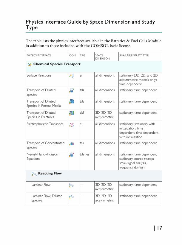
The table lists the physics interfaces available in the Batteries & Fuel Cells Module in addition to those included with the COMSOL basic license.

PHYSICS INTERFACE ICON TAG SPACE DIMENSION

AVAILABLE STUDY TYPE

Chemical Species Transport

Surface Reactions sr all dimensions stationary (3D, 2D, and 2D axisymmetric models only); time dependent

Transport of Diluted Species

tds all dimensions stationary; time dependent

Transport of Diluted Species in Porous Media

tds all dimensions stationary; time dependent

Transport of Diluted Species in Fractures

dsf 3D, 2D, 2D axisymmetric

stationary; time dependent

Electrophoretic Transport el all dimensions stationary; stationary with initialization; time dependent; time dependent with initialization

Transport of Concentrated Species

tcs all dimensions stationary; time dependent

Nernst-Planck-Poisson Equations

tds+es all dimensions stationary; time dependent; stationary source sweep; small-signal analysis, frequency domain

Reacting Flow

Laminar Flow — 3D, 2D, 2D axisymmetric

stationary; time dependent

Laminar Flow, Diluted Species

— 3D, 2D, 2D axisymmetric

stationary; time dependent

| 17

Reacting Flow in Porous Media

Transport of Diluted Species

rfds 3D, 2D, 2D axisymmetric

stationary; time dependent

Transport of Concentrated Species

rfcs 3D, 2D, 2D axisymmetric

stationary; time dependent

Electrochemistry

Primary Current Distribution

Secondary Current Distribution

cd all dimensions stationary; stationary with initialization; time dependent; time dependent with initialization; AC impedance, initial values; AC impedance, stationary; AC impedance, time dependent

Tertiary Current Distribution, Nernst-Planck (Electroneutrality, Water-Based with Electroneutrality, Supporting Electrolyte)

tcd all dimensions stationary; stationary with initialization; time dependent; time dependent with initialization; AC impedance, initial values; AC impedance, stationary; AC impedance, time dependent

Electroanalysis elan all dimensions stationary; time dependent; AC impedance, initial values; AC impedance, stationary; AC impedance, time dependent; cyclic voltammetry

Electrode, Shell els 3D, 2D, 2D axisymmetric

stationary; time dependent

Battery Interfaces

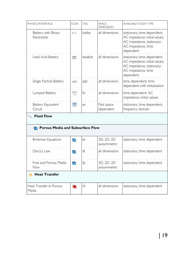
Lithium-Ion Battery liion all dimensions stationary; time dependent; AC impedance, initial values; AC impedance, stationary; AC impedance, time dependent

PHYSICS INTERFACE ICON TAG SPACE DIMENSION

AVAILABLE STUDY TYPE

18 |

Battery with Binary Electrolyte

batbe all dimensions stationary; time dependent; AC impedance, initial values; AC impedance, stationary; AC impedance, time dependent

Lead Acid Battery leadbat all dimensions stationary; time dependent; AC impedance, initial values; AC impedance, stationary; AC impedance, time dependent

Single Particle Battery spb all dimensions time dependent; time dependent with initialization

Lumped Battery lb all dimensions time dependent; AC impedance, initial values;

Battery Equivalent Circuit

ec Not space dependent

stationary; time dependent; frequency domain

Fluid Flow

Porous Media and Subsurface Flow

Brinkman Equations br 3D, 2D, 2D axisymmetric

stationary; time dependent

Darcy’s Law dl all dimensions stationary; time dependent

Free and Porous Media Flow

fp 3D, 2D, 2D axisymmetric

stationary; time dependent

Heat Transfer

Heat Transfer in Porous Media

ht all dimensions stationary; time dependent

PHYSICS INTERFACE ICON TAG SPACE DIMENSION

AVAILABLE STUDY TYPE

| 19

Tutorial of a Lithium-Ion Battery

The following is a two-dimensional model of a lithium-ion battery. The cell geometry could be a small part of an experimental cell but here it is only meant to demonstrate a 2D model setup. The battery contains a positive porous electrode, electrolyte, a negative lithium metal electrode and a current collector. This cell configuration is sometimes called a “half-cell”, since the lithium metal electrode is usually considered to have negligible impact on cell voltage and polarization. A realistic 2D geometry is shown in the model Edge Effects in a Spirally Wound Li-Ion Battery available in the Batteries & Fuel Cells Module application library.

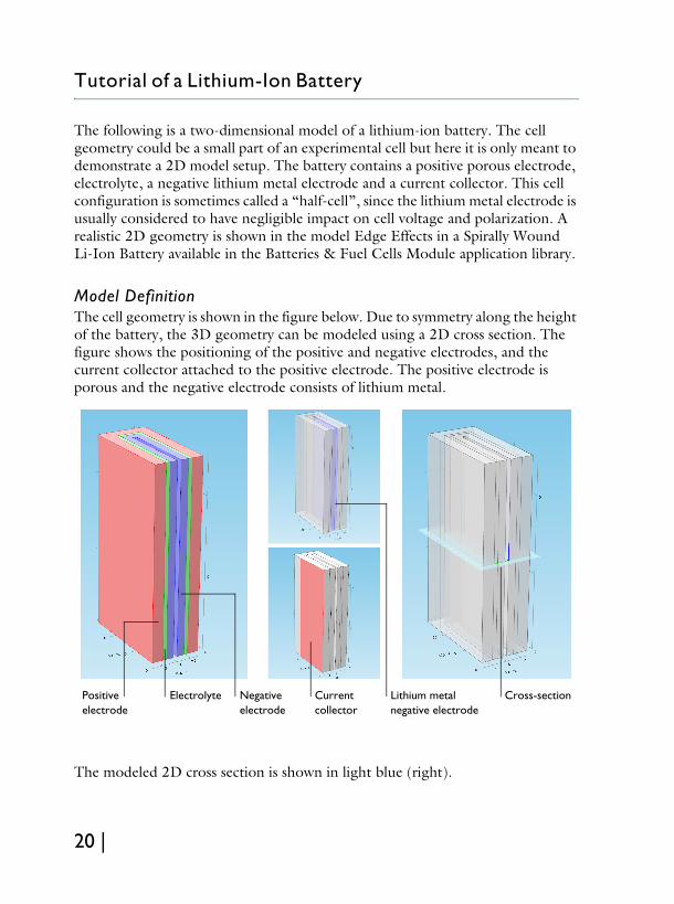
Model DefinitionThe cell geometry is shown in the figure below. Due to symmetry along the height of the battery, the 3D geometry can be modeled using a 2D cross section. The figure shows the positioning of the positive and negative electrodes, and the current collector attached to the positive electrode. The positive electrode is porous and the negative electrode consists of lithium metal.

The modeled 2D cross section is shown in light blue (right).

Positive electrode

Electrolyte Negative electrode

Cross-sectionCurrent collector

Lithium metal negative electrode

20 |

Since the electrochemical reaction only takes place at the surface of the lithium metal which is in contact with electrolyte in the separator, and the electronic conductivity is very high compared to the porous positive electrode, the thickness of the metal can be neglected in the model geometry. The modeled 2D cell geometry is shown in the figure below. During discharge, the positive electrode acts as the cathode and the contact of the metallic tab acts as a current collector. The negative lithium metal electrode acts as the anode and current feeder.

The model defines and solves the current and material balances in the lithium-ion battery. The intercalation of lithium inside the particles in the positive electrode is solved using a fourth independent variable r for the particle radius (x, y, and t are the other three). The reaction kinetics and the intercalation are coupled to the material and current balances at the surface of the particles. The model equations are found in the Batteries & Fuel Cells Module User’s Guide. The model was originally formulated for 1D simulations by John Newman and his co-workers at the University of California at Berkeley.

Results and DiscussionThe purpose of the 2D simulation is to reveal the distribution of the depth of discharge in the positive electrode, as a function of discharge time. This distribution depends on the positioning of the current collector and the thickness of the positive electrode and electrolyte layer, in combination with the electrode kinetics and transport properties.The figure below shows the concentration of lithium at the surface of the positive electrode particles in the electrodes after 2700 s of discharge at 0.05 A.

Current collector

Positive electrode

(porous)

Negative electrode

(solid lithium metal)

1.3 mm

| 21

The high concentration at the positive electrodes is proportional to the local depth of discharge of these parts of the electrode. The figure shows that the back side of the electrode, with respect to the position of the current collector, is less utilized during discharge. As the discharge process continues, these parts will subsequently discharge. However, for repeated cycling of the cell (charge and discharge), the different parts of the electrodes will age in a nonuniform way if the electrodes are only discharged to a moderate degree during cycling

Despite the simplicity of this model, it shows a problem that may arise in realistic battery geometry if the shape and configuration of the electrodes, current collectors, and current feeders are not investigated thoroughly using modeling and simulations.The following instructions show how to formulate, solve, and reproduce this model.

Model Wizard

Note: These instructions are for the user interface on Windows but apply, with minor differences, also to Linux and Mac.

22 |

1 To start the software, double-click the COMSOL icon on the desktop or Start menu of the computer. When the software opens, you can choose to use the Model Wizard to create a new COMSOL model or Blank Model to create one manually. For this tutorial, click the Model Wizard button.If COMSOL is already open, you can start the Model Wizard by selecting New from the File menu and then click Model Wizard .

The Model Wizard guides you through the first steps of setting up a model. First you select the dimension of the modeling space.

2 In the Space Dimension window click the 2D button .3 On the Select Physics tree under Electrochemistry>Battery Interfaces,

double-click Lithium-Ion Battery (liion) to add it to the Added physics interfaces list.

4 Click Study .5 On the Studies window under Preset Studies, click Time Dependent with

Initialization . This study type simplifies the modeling, since it reduces the number of initial values that need to be set by computing the initial potentials in the battery interface.

6 Click Done .

Geometry 1

Insert a prepared geometry sequence from a file. After insertion you can study each geometry step in the sequence.1 On the Geometry toolbar, click Insert Sequence.2 Browse to the file li_battery_tutorial_2d_geom_sequence.mph in the

application library folder on your computer, Batteries_and_Fuel_Cells_Module\Batteries,_Lithium-Ion. Double-click to add or click Open.

3 On the Geometry toolbar, click Build All.

| 23

Note: The location of the file used in this exercise varies based on the installation of COMSOL Multiphysics. For example, if the installation is on your hard drive, the file path might be similar to C:\Program Files\COMSOL54\applications\.

Materials

Use the Batteries and Fuel Cells material library to set up the material properties for the electrolyte and electrode (anode and cathode) materials. By adding the electrolyte material to the model first, this material becomes the default material for all domains.

1:2 EC:DMC and p(VdF-HFP) (Polymer electrolyte, Li-ion Battery)1 On the Home toolbar, click Add Material .

24 |

2 Go to the Add Material window. In the tree under Batteries and Fuel Cells, under Electrolytes right-click LiPF6 in 1:2 EC:DMC and p(VdF-HFP) (Polymer electrolyte, Li-ion Battery) and choose Add to Component1.

LMO Electrode, LiMn2O4 Spinel (Positive, Li-ion Battery)1 Go to the Add Material window.2 In the tree under Batteries and Fuel Cells under Electrodes click LMO

Electrode, LiMn2O4 Spinel (Positive, Li-ion Battery). . In the Add Material window click Add to Component.

The node sequence in the Model Builder under the Materials node should match this figure.

The first material (LiPF6...) was assigned by default to all domains. Override this default selection by assigning the electrode material to domain 1.3 On the LMO Electrode, LiMn2SO4 Spinel (Positive, Li-ion Battery), select

Domain 1.The LMO material node will now be marked with a small red cross in the model tree, indicating missing material properties. This is expected at this point and will be resolved when setting up the physics for the porous electrode node.If you want you may now click, expand and inspect the various properties present in the nodes you under Materials (cEeqref denotes the maximum Li concentration in the active material). Most of these properties will be used by the physical model you will now proceed to define.

| 25

Lithium-Ion Battery Interface

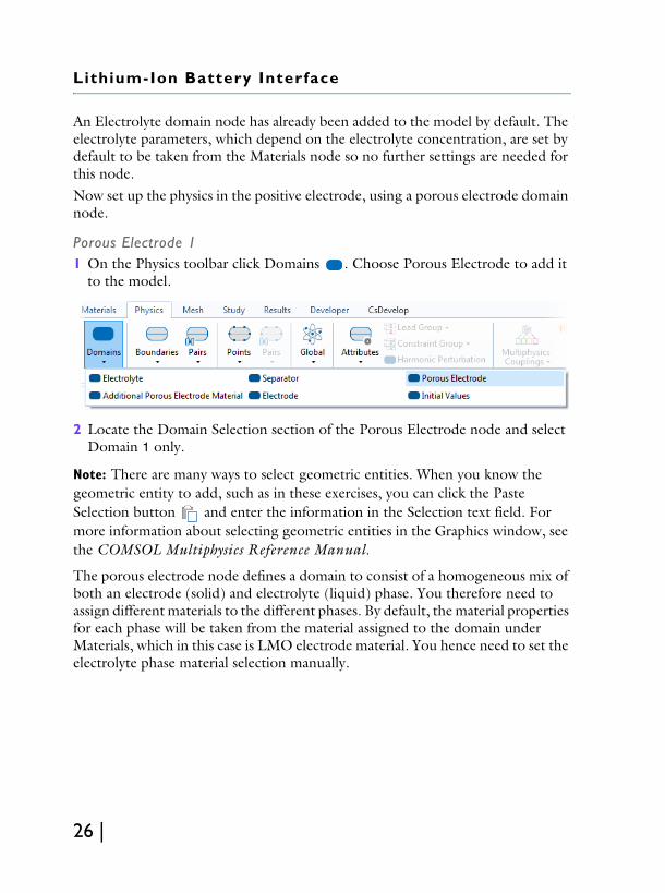
An Electrolyte domain node has already been added to the model by default. The electrolyte parameters, which depend on the electrolyte concentration, are set by default to be taken from the Materials node so no further settings are needed for this node. Now set up the physics in the positive electrode, using a porous electrode domain node.

Porous Electrode 11 On the Physics toolbar click Domains . Choose Porous Electrode to add it

to the model.

2 Locate the Domain Selection section of the Porous Electrode node and select Domain 1 only.

Note: There are many ways to select geometric entities. When you know the geometric entity to add, such as in these exercises, you can click the Paste Selection button and enter the information in the Selection text field. For more information about selecting geometric entities in the Graphics window, see the COMSOL Multiphysics Reference Manual.

The porous electrode node defines a domain to consist of a homogeneous mix of both an electrode (solid) and electrolyte (liquid) phase. You therefore need to assign different materials to the different phases. By default, the material properties for each phase will be taken from the material assigned to the domain under Materials, which in this case is LMO electrode material. You hence need to set the electrolyte phase material selection manually.

26 |

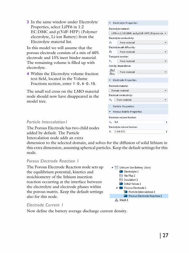
3 In the same window under Electrolyte Properties, select LiPF6 in 1:2 EC:DMC and p(VdF-HFP) (Polymer electrolyte, Li-ion Battery) from the Electrolyte material list.

In this model we will assume that the porous electrode consists of a mix of 40% electrode and 15% inert binder material. The remaining volume is filled up with electrolyte.4 Within the Electrolyte volume fraction

text field, located in the Volume Fractions section, enter 1-0.4-0.15.

The small red cross on the LMO material node should now have disappeared in the model tree.

Particle Intercalation1The Porous Electrode has two child nodes added by default. The Particle Intercalation node adds an extra dimension to the selected domain, and solves for the diffusion of solid lithium in this extra dimension, assuming spherical particles. Keep the default settings for this node.

Porous Electrode Reaction 1The Porous Electrode Reaction node sets up the equilibrium potential, kinetics and stoichiometry of the lithium insertion reaction occurring at the interface between the electrolyte and electrode phases within the porous matrix. Keep the default settings also for this node.

Electrode Current 1Now define the battery average discharge current density.

| 27

1 On the Physics toolbar click Boundaries and choose Electrode Current .

2 Select boundary 10 only.3 In the Electrode Current section, select Average current density in the list and

enter -50[A/m2] in the average current density text field.

Electrode Surface 1Finish the model by defining the negative electrode. Due to the high conductivity of the lithium metal it suffices to define the electrode surface between the lithium metal domain (not included in the model geometry) and the electrolyte domain (included in the model geometry). 1 On the Physics toolbar click Boundaries and choose Electrode Surface .

2 Select Boundary 5, 7, and 12 only.

28 |

The metal potential of the electrode is grounded (set to 0 V) by default so no further settings are needed for this node.

Electrode Reaction 1Similar to the Porous Electrode node, the Electrode Surface node comes with a default Electrode Reaction subnode. Expand the Electrode Surface node and inspect the various settings of the subnode. The equilibrium potential inputs need to be set to values that are applicable for a lithium metal surface.

Electrode Reaction11 In the Model Builder, expand the Electrode Surface 1 node and click the

Electrode Reaction 1 node .2 Under Equilibrium Potential select User

defined for the Equilibrium potential. Enter 0 in the V text field.

3 In the same window under Heat of Reaction, select User defined for the Temperature derivative of equilibrium potential. Enter 0 in the V/K text field.

The values of 0 V and 0 V/K for the two inputs, respectively, are applicable for a lithium metal surface.

Mesh 1

In this example the automatically generated mesh is used so no manual mesh settings are required. You may inspect the automatically generated mesh as follows:

| 29

1 In the Model Builder window, under Component 1 (comp1) right-click Mesh 1 and choose Build All.

Study 1

Set up a 2700 second time-dependent solver to store the solution at 10 second intervals during the first 100 seconds, and 100 second intervals during the last 2600 seconds. Then solve the problem.

Step 2: Time Dependent1 In the Model Builder expand the Study 1 node and click Step 2: Time

Dependent .2 In the Settings window for Time Dependent, locate the Study Settings section.

30 |

3 Click Range (the small icon to the right of the Times text field).

4 In the Range dialog box, type 10 in the Step text field.

5 In the Stop text field, type 100.6 Click Replace.7 Click Range again and type 200 in the Start text

field.8 In the Step text field, type 100.9 In the Stop text field, type 2700.10Click Add.(Alternatively, you may also type in the expression range(0,10,100) range(200,100,2700) directly in the Times text field.)

11On the Home toolbar click Compute .

Results

Boundary Electrode Potential vs Ground (liion)A plot of the electrode voltage where you set the Electrode Current condition is created by default. Since you grounded the other electrode this equals the battery voltage during the simulation.1 In the Model Builder window, under Results click Boundary Electrode

Potential vs Ground (liion).

| 31

2 Rename the plot group by typing Battery Voltage in the Label text field available in the Settings window, click Plot .

Also browse through the other default plots created. For the 2D plots you can select the time to plot for in the Data section.

2D Plot Group 8The following steps create a plot of the solid lithium concentration at the surface of the electrode particles at 2700 seconds.1 On the Home toolbar, click Add Plot Group and choose 2D Plot

Group .2 Rename the plot group by typing Lithium concentration on Particle Surface in the Label text field available in the Settings window.

3 On the Lithium concentration on Particle Surface toolbar click Surface .

4 In the Settings window for Surface click Replace Expression (it is in the upper-right corner of the Expression section). Choose Insertion particle concentration, surface (liion.cs_surface), under the Particle Intercalation menu.

5 On the Lithium concentration on Particle Surface toolbar click Plot .

32 |

6 On the Graphics toolbar click the Zoom Extents button .

Data SetsAs mentioned before, the Particle Intercalation node adds an extra dimension to the porous electrode domain, and solves for the concentration of solid lithium in this extra dimension. To create a plot of the lithium concentration in the particles in the positive electrode you need to first create a Solution data set that refers to the extra dimension.1 On the Results toolbar, click More Data Sets and choose Solution .2 In the Solution Settings window, choose Extra Dimension from Porous

Electrode 1 (liion_pce1_pin1_xdim) in the Component list displayed within the Solution section.

1D Plot Group 9Start with the settings to plot the solid lithium concentration in the negative electrode.1 On the Results toolbar, click 1D Plot Group .2 Rename the plot group by typing Lithium Concentration in Positive Electrode Particles in the Label text field available in the Settings window.

3 In the Settings window for 1D Plot Group, choose None from the Data set list located in the Data section.

| 33

4 On the Lithium Concentration in Particle toolbar, click Line Graph .5 In the Settings window for Line Graph,

find the Data set list in the Data section and choose Study 1/Solution 1 (3).

6 From the Time selection list, choose Last to plot only the last time step of the solution.

7 From the Selection list in the Selection section, choose All domains.

8 The atxd2() operator is used to specify the x and y coordinates in the battery geometry and the variable that is plotted. In the Expression text field of the y-Axis Data section, type comp1.atxd2(5e-4,1e-4,liion.cs_pce1).

9 Create Legends in the plot:10Click to expand the Legends section.

Select the Show legends check box.11From the Legends list, choose Manual

and enter x=0.5 mm, y=0.1 mm in the table.

12Right-click Line Graph 1 and choose Duplicate to plot the concentration in an additional location within the positive electrode.

13In the Settings window for Line Graph, locate the y-Axis Data section.

14In the Expression text field of the y-Axis Data section, type comp1.atxd2(5e-4,5.5e-4,liion.cs_pce1).

15Click to expand the Legends section and replace the text in the table with x=0.5 mm, y=0.55 mm.

34 |

16To finalize the plot group, return to the Lithium Concentration in Particle toolbar node by clicking it in the Model Builder.

17In the Settings window for 1D Plot Group, click to expand the Title section, where you choose Manual from the Title type list.

18In the Title text area, enter Lithium Concentration Positive Electrode Particles, t=2700 s.

19In the Plot Settings section:- Select the x-axis label check box and type in the associated text field Normalized Particle Dimension.

- Select the y-axis label check box and type Lithium Concentration (mol/m³).

20Click to expand the Legend section, choose Upper left from the Position list.21Click the Zoom Extents button on the Graphics toolbar and click Plot

on the Lithium Concentration in Particle toolbar.

| 35

Tutorial of a Fuel Cell Cathode

One of the most important—and most difficult—phenomena is to model mass transport through gas diffusion and reactive layers in a fuel cell. Gas concentrations are often large and are significantly affected by the reactions that take place. This makes Fickian diffusion an inappropriate assumption to model the mass transport.Figure 8 shows an example 3D geometry of a cathode from a fuel cell with perforated current collectors. It is often seen in self-breathing cathodes or in small experimental cells. Due to the perforation layout, a 3D model is needed in the study of the mass transport, current, and reaction distributions.

Figure 8: A fuel cell cathode with a perforated current collector.

This model investigates such a geometry and the mass transport that occurs through Maxwell-Stefan diffusion. It couples this mass transport to Tafel-like electrochemical kinetics in the reaction term at a cathode.The electrochemical reaction for a PEM fuel cell to produce electrical energy is given by:

At the anode Hydrogen Oxidation Reaction (HOR) yield protons:

Gas inlet hole

Unit cell

Reactive layer

Electrolyte layer

H212---O2

-+ H2O-→ Eeq 1.23= V

36 |

water is produced via Oxygen Reduction Reaction (ORR):

Model DefinitionFigure 9 shows details for a unit cell from Figure 8. The circular hole in the collector is where the gas enters the modeling domain, where the composition is known. The upper rectangular domain is the reaction-zone electrode. It is a porous structure that contains the feed-gas mixture, an electronically conducting material covered with an electrocatalyst, and an electrolyte. The lower domain corresponds to a free electrolyte ionically connecting the two electrodes of the fuel cell. No reaction takes place in this domain. Neither are there pores to allow gas to flow or material for electronic current—current is conducted ionically.The reaction zone is 0.075 mm thick, as is the electrolyte layer. The unit cell is 1.5-by-1.5 mm in surface, and the gas inlet hole has a radius of 1.0 mm.

Figure 9: The modeled fuel cell cathode unit cell. The marked zone is the surface of the cathode that is open to the feed gas inlet, while the rest of the top surface sits flush against the current collector. In the unit cell the top domain is the porous cathode, while the bottom domain is the free electrolyte.

The electronic and ionic current balances are modeled using a Secondary Current Distribution interface.The species (mass) transport is modeled by the Maxwell-Stefan equations for oxygen (Species 1) and water (Species 2) in the gas phase using a Transport of

H2 2H+ 2e-+→ Eeq 0= V

12---O

22H+ 2e-

+ + H2O→ Eeq 1.23= V

| 37

Concentrated Species interface. Mass transport is solved for in the electrode domain only. The velocity vector is solved for using a Darcy’s Law interface.

Results and DiscussionFigure 10 shows the oxygen concentration at a total potential drop over the modeled domain of 190 mV. The figure shows that concentration variations are small along the thickness of the cathode for this relatively small current density, while they are substantially larger along the electrode’s width.

Figure 10: Isosurfaces of the weight fraction of oxygen at a total potential drop over the modeled domain of 190 mV.

Figure 11 shows the gas velocity in the porous cathode. There is a significant velocity peak at the edge of the inlet orifice. This is caused by the contributions of the reactive layer underneath the current collector because in this region the convective flux dominates the mass transport. Thus it is important to model the velocity field properly. In this case, the combination of a circular orifice and square unit cell eliminates the possibility to approximate the geometry with a rotationally symmetric model.The electrochemical reaction rate, represented by the local current density, is related to both the local overpotential and oxygen concentration. Figure 12 depicts the local overpotential, which is rather even throughout the cathode. This is

38 |

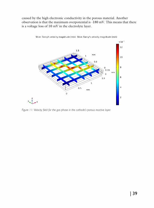
caused by the high electronic conductivity in the porous material. Another observation is that the maximum overpotential is -180 mV. This means that there is a voltage loss of 10 mV in the electrolyte layer.

Figure 11: Velocity field for the gas phase in the cathode’s porous reactive layer.

| 39

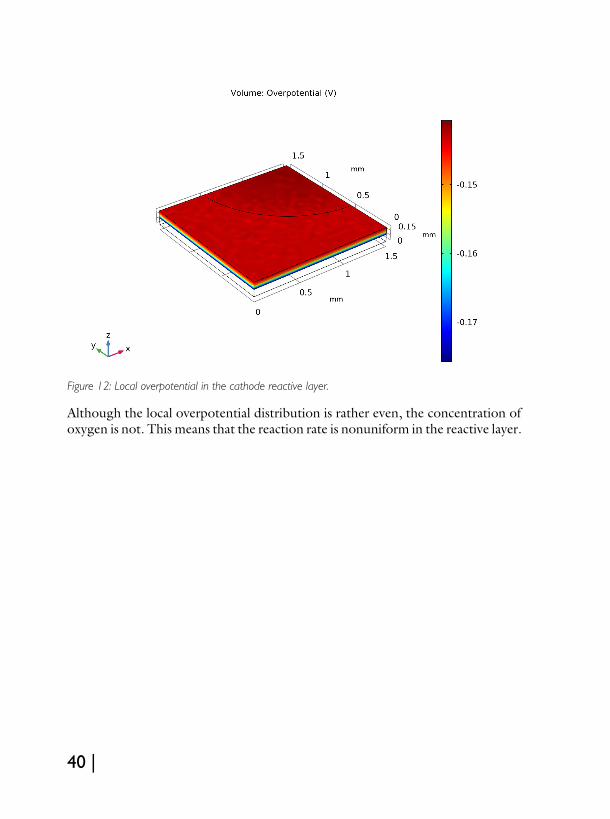
Figure 12: Local overpotential in the cathode reactive layer.

Although the local overpotential distribution is rather even, the concentration of oxygen is not. This means that the reaction rate is nonuniform in the reactive layer.

40 |

One way to study the distribution of the reaction rate is to plot the ionic current density at the bottom boundary of the free electrolyte. Figure 13 shows such a plot.

Figure 13: Current density perpendicular to the lower, free electrolyte boundary.

The current-density distribution shows that the variations are rather large. The reaction rate and the current production are higher beneath the orifice and decrease as the distance to the gas inlet increases. This means that the mass transport of reactant dictates the electrode’s efficiency for this design at these particular conditions.The following instructions show how to formulate, solve, and reproduce this model.

Model Wizard

Start by adding a Secondary Current Distribution interface and a Stationary study to set up and solve for a current distribution model of the cell. Later you will add more physics features for modeling mass transport and convection.1 If COMSOL is already open, you can start the Model Wizard by selecting

New from the File menu and then click Model Wizard .2 In the Space Dimension window click the 3D button .

| 41

3 In the Select Physics tree under Electrochemistry>Primary and Secondary Current Distribution, click Secondary Current Distribution (cd) .

4 Click Add and then click the Study button.5 Under General Studies, click Stationary . 6 Click Done .

Geometry 1

Now draw the model geometry. Use blocks to define the electrolyte and the porous electrode domains. Then use a workplane to draw the inlet hole at the top of the porous electrode. Facilitate geometry selection later (when setting up the physics interfaces) by enabling Create Selections and renaming the geometry objects.Begin by setting the default length unit to millimeters.1 In the Model Builder under Component 1, click Geometry 1 .2 In the Settings window for Geometry locate the Units section. From the

Length unit list, choose mm.

Create the First Block1 On the Geometry toolbar click Block .

2 In the Model Builder under Geometry 1, click Block 1 .3 In the Settings window for Block locate

the Size section.- In the Width text field, type 1.5.- In the Depth text field, type 1.5.- In the Height text field, type 0.075.

4 Locate the Selections of Resulting Entities section. Select the Resulting objects selections check box. From Show in physics choose Domain selection. This enables the geometry to be chosen as a domain while setting physics later (similar to Explicit).

5 Right-click Block 1 and choose Rename (or press F2).

42 |

6 Go to the Rename Block dialog box and type Electrolyte in the New name text field. Click OK.

7 Click the Build Selected button .

Duplicate the Block and Change z Position1 Right-click Electrolyte and choose Duplicate .

2 In the Settings window for Block locate the Position section. In the z text field, type 0.075.

3 Click the Electrolyte 1 node and press F2.4 Go to the Rename Block dialog box and type Porous Electrode in the New

name text field. Click OK.

| 43

Create a Work Plane for Drawing the Inlet Hole1 On the Geometry toolbar click Work Plane .

2 In the Model Builder click Work Plane 1 .3 In the Settings window for Work Plane locate the Plane Definition section. In

the z-coordinate field, type 0.15.4 Locate the Selections of Resulting Entities section. Select the Resulting objects

selections check box. From Show in physics choose Boundary selection. This enables the geometry to be chosen as a boundary while setting physics later (similar to Explicit).

5 Right-click Work Plane 1 and choose Rename (or click the node and press F2).

6 Go to the Rename Work Plane dialog box and type Inlet in the New name text field. Click OK.

Draw the Inlet Hole1 In the Model Builder under Geometry 1>Inlet, right-click Plane Geometry and

choose Circle .

44 |

2 In the Settings window for Circle locate the Size and Shape section.- In the Radius text field, type 1.- In the Sector angle text field, type 90.

3 Locate the Position section.- In the xw text field, type 1.5.- In the yw text field, type 1.5.

4 Locate the Rotation Angle section. In the Rotation text field, type 180.

5 Click the Build Selected button .

Form a Union to Finalize the Geometry1 In the Model Builder click the Form Union node and then click the Build

Selected button . 2 Click the Zoom Extents button on the Graphics toolbar.

| 45

Your finished geometry should look like this:

Global Definit ions

Load the model parameters from a text file.

Parameters1 On the Home toolbar click Parameters and select Parameters 1 .

Note: On Linux and Mac, the Home toolbar refers to the specific set of controls near the top of the Desktop.

46 |

2 In the Settings window for Parameters locate the Parameters section. Click Load from File .

3 In the application library folder on your computer, applications\Batteries_and_Fuel_Cells_Module\Fuel_Cells, double-click the file fuel_cell_cathode_parameters.txt to import it to the Parameters table. Note that the location of the files used in this exercise may vary depending on the installation. For example, if the installation is on your hard drive, the file path might be similar to C:\Program Files\COMSOL54\applications\.

SelectionsNow manually add selections for the bottom electrolyte and top current collector boundaries.1 On the Definitions toolbar in the Selections section, click Explicit .

2 In the Model Builder under Definitions, click Explicit 1 .3 In the Settings window for Explicit locate the Input Entities section. From the

Geometric entity level list, choose Boundary.4 Select Boundary 3 only.5 Click Explicit 1 and press F2. 6 Go to the Rename Explicit dialog box and type Electrolyte Boundary in the

New name text field. Click OK.

Add a selection for the Current Collector in a similar way.1 On the Definitions toolbar in the Selections section, click Explicit .2 In the Model Builder click Explicit 2 .3 In the Settings window for Explicit locate the Input Entities section. From the

Geometric entity level list, choose Boundary.

| 47

4 Select Boundary 7 only, e.g. by using Paste Selection .5 Click Explicit 2 and press F2.6 Go to the Rename Explicit dialog box and type Current Collector in the

New name text field. Click OK.

Secondary Current Distribution

Now start defining the physics interface for the current distribution model. Add a porous electrode and specify the electrode reaction parameters, then add potential boundary nodes for both the electrolyte and the electrode phase. Note that an Electrolyte node already has been added automatically by default.

Porous Electrode 11 On the Physics toolbar click Domains and choose Porous Electrode .2 In the Model Builder under Secondary Current Distribution , click Porous

Electrode 1 . Keep the default From material setting for the conductivities in this node (the Materials node is specified later.)

3 In the Settings window for Porous Electrode, locate the Domain Selection section and select Porous Electrode.

4 From the Effective conductivity correction list, choose No correction in both the Electrolyte Current Conduction and the Electrode Current Conduction sections.

48 |

Porous Electrode Reaction 11 In the Model Builder expand the Porous Electrode 1 node, then click Porous

Electrode Reaction 1 .

2 In the Settings window for Porous Electrode Reaction locate the Model Inputs section. In the T text field, type T.

3 Locate the Electrode Kinetics section. - From the Kinetics expression type list,

choose Butler-Volmer.- In the i0 text field, type i0.

4 Locate the Active Specific Surface Area section. In the av text field, type S.

Electrolyte Potential 11 On the Physics toolbar click Boundaries

and choose Electrolyte Potential .

2 In the Model Builder under Secondary Current Distribution , click Electrolyte Potential 1 .

3 Locate the Boundary Selection section. From the Selection list choose Electrolyte Boundary.

Electric Potential 11 On the Physics toolbar click Boundaries

and choose Electric Potential .

| 49

2 In the Model Builder under Secondary Current Distribution , click Electric Potential 1 .

3 In the Settings window for Electric Potential, locate the Boundary Selection section. Choose Current Collector from the Selection list.

4 Locate the Electric Potential section. In the φs,bnd text field, type E_pol.

Initial Values 1Also provide initial values for the potentials. This reduces the computational time.1 In the Model Builder under Secondary Current Distribution , click Initial

Values 1 .2 In the Settings window for Initial Values, locate the Initial Values section. In the

phis text field, type E_pol.

Materials

The Materials node is marked in red. This indicates that there are material parameters missing in the model. Add two different material nodes for the electrolyte and the porous electrode, and specify the conductivity values.

Material 1 (Electrolyte)1 In the Model Builder, under Component 1, right click on Materials and

click Blank Material .

50 |

2 In the Settings window for Material locate the Geometric Entity Selection section. Choose Domain from Geometric entity level. From the Selection list choose Electrolyte.

3 Locate the Material Contents section. In the table enter the following settings:

Material 2 (Porous Electrode)1 In the Model Builder, under Component 1, right click on Materials and

click Blank Material .2 In the Settings window for Material locate the Geometric Entity Selection

section. From the Selection list choose Porous Electrode.3 Locate the Material Contents section. In the table enter the following settings:

Note: You can provide the conductivities in the table either directly by typing in the values or by using parameters defined in the Parameters node.

PROPERTY NAME VALUE

Electrolyte conductivity sigmal 5[S/m]

PROPERTY NAME VALUE

Electrolyte conductivity sigmal 1[S/m]

Electrical conductivity sigma sigma_s

| 51

Mesh 1

Use the default mesh sequence that is induced by the physics interface but change to a finer size.1 In the Model Builder click Mesh 1 .2 In the Settings window for Mesh locate the Mesh Settings section. From the

Element size list choose Fine.3 Click the Build All button .

52 |

The finished mesh should now look like this:

Study 1

The current distribution model is now ready for solving.1 On the Home toolbar click Compute .

Results

Electrolyte potential plots are created by default. Now create a plot of the local overpotential by first adding a plot group followed by a volume plot.

3D Plot Group 51 On the Home toolbar click Add Plot Group and choose 3D Plot Group .

| 53

2 On the 3D Plot Group 5 toolbar click Volume .

3 Click Volume 1 .

4 In the Settings window for Volume click Replace Expression (it is in the upper-right corner of the Expression section). Choose Secondary Current Distribution>Electrode kinetics>Overpotential (cd.eta_per1).

54 |

5 On 3D plot group, scroll to Color Legend and choose Right from Position menu. Click the Plot button . The overpotential plot should now look like this:

6 In the Model Builder right-click 3D Plot Group 5 and choose Rename.7 Go to the Rename 3D Plot Group dialog box and type Local Overpotential

in the New name text field. Click OK.

3D Plot Group 61 On the Home toolbar click Add Plot Group and choose 3D Plot Group .2 Click 3D Plot Group 6 .

3 On the 3D Plot Group 6 toolbar click Surface .4 In the Settings window for Surface click Replace Expression and choose

Normal electrolyte current density (cd.nIl). You can use operators to modify any postprocessing variable. In this case, use the abs() function to plot the absolute value of the current density.

5 Locate the Expression section. In the Expression text field, type abs(cd.nIl).

| 55

Selection 11 Right-click Results>3D Plot Group 6>Surface 1 and choose Selection.

2 Select Boundary 3 only.

3 On the 3D Plot Group toolbar click Plot .

The current density plot should now look like this:

4 Click 3D Plot Group 6 and press F2.5 Go to the Rename 3D Plot Group dialog box and type Electrolyte Current Density in the New name text field. Click OK.

Change Element Order and Recompute

Now change to second-order elements in the finite element discretization. This will increase the accuracy of the solution and render a smoother plot. (Alternatively, you could increase the resolution of the mesh).1 In the Settings window for Secondary Current Distribution , click to expand

the Discretization section.2 From the Electrolyte potential list, choose Quadratic.3 From the Electric potential list choose Quadratic.

56 |

4 On the Home toolbar click Compute .

The current density plot should now look like this:

Add Mass Transport and Fluid Flow Physics Features to the Model

Now, add more physics features to the model by adding a Transport of Concentrated Species interface for gas phase mass transport and a Darcy’s Law interface for the convective flow.1 On the Home toolbar click Add Physics .2 Go to the Add Physics window. In the tree under Chemical Species Transport,

click Transport of Concentrated Species .3 Click to expand the Dependent variables section. In the Number of species text

field, type 3. In the Mass fractions table, enter w_n2, w_o2,and w_h2o.4 In the Add Physics window click Add to Component.5 Go to the Add Physics window again. In the tree under Fluid Flow>Porous

Media and Subsurface Flow, click Darcy’s Law .6 In the Add physics window click Add to Component.

| 57

Transport of Concentrated Species

Now define the settings for the mass transport of nitrogen, oxygen and water.1 In the Model Builder click Transport of Concentrated Species .

2 Locate the Domain Selection section. From the Selection list choose Porous Electrode.

3 Locate the Transport Mechanisms section. From the Diffusion model list choose Maxwell-Stefan.

Transport Properties 11 In the Model Builder expand the Transport of Concentrated Species node

then click Transport Properties 1 .2 In the Settings window for Transport Properties, locate the Density section.

- In the Mw_n2 text field, type M_n2.- In the Mw_o2 text field, type M_o2.- In the Mw_h2o text field, type M_h2o.

58 |

3 Locate the Diffusion section. From the Binary diffusion input type list, choose Matrix. In the Dik table enter the following settings:

4 Both the velocity and pressure are coupled to Darcy's law. This will be done later using the Flow Coupling Multiphysics feature. Locate the Model Inputs section.- Locate the Model Input section. In

the T text field, type T.- Locate the Convection section. From

the u list, choose Darcy's velocity field (dl).

- In the Model Builder window, click Transport of Concentrated Species (tcs).

- In the Settings window for Transport of Concentrated Species, locate the Transport Mechanisms section.

- Select the Mass transfer in porous media check box.

1 D_o2n2_eff D_n2h2o_eff

D_o2n2_eff 1 D_o2h2o_eff

D_n2h2o_eff D_o2h2o_eff 1

| 59

Couple the Reaction Rate of Oxygen to the Electrochemical CurrentsUse a porous electrode coupling to create a mass sink in the domain corresponding to the oxygen leaving the gas phase due to the electrochemical reactions.1 On the Physics toolbar click Domains and choose Porous Electrode

Coupling .2 Click Porous Electrode Coupling 1 . 3 In the Settings window for Porous Electrode Coupling locate the Domain

Selection section. From the Selection list choose Porous Electrode.4 Expand the Porous Electrode Coupling node and click Reaction Coefficients 1

.

5 In the Settings window for Reaction Coefficients, locate the Model Inputs section. From the iv list, choose Local current source, Porous Electrode Reaction 1 (cd/pce1/per1).

6 Locate the Stoichiometric Coefficients section. - In the n text field, type 4.- In the νw_o2 text field, type -1.- In the νw_h2o text field, type 2.

Define the Initial Values Node1 Click the Initial Values 1 node . 2 In the Settings window under Initial Values, enter Mass fraction values w_o2_ref in the w0,wo2 field and w_h2o_ref in the w0,wh2o field.

Define the Inflow Node1 On the Physics toolbar click Boundaries and choose Inflow . 2 In the Model Builder click Inflow 1 .3 In the Settings window for Inflow locate the Boundary Selection section. From

the Selection list choose Inlet.4 Locate the Inflow section.

- In the w0,wo2 text field, type w_o2_ref.- In the w0,wh2o text field, type w_h2o_ref.

60 |

Darcy's Law

Now do the settings for Darcy's law. Also here the electrochemical currents result in a mass sink due to the oxygen molecules leaving the domain.1 In the Model Builder click Darcy's Law .

2 In the Settings window for Darcy's Law locate the Domain Selection section. From the Selection list, choose Porous Electrode.

3 Locate the Physical Model section. In the pref text field, type p_atm.

Define the Fluid and Matrix Properties1 Expand the Darcy's Law (dl) node then click Fluid and Matrix Properties 1. 2 Locate the Fluid Properties section.

- From the ρ list, choose Density (tcs/cdm1). (The density is now taken from the Transport of Concentrated Species interface.)

- From the μ list, choose User defined. In the associated text field, type mu.

3 Locate the Matrix Properties section. - From the εp list, choose User defined.

In the associated text field, type e_por.

- From the κ list, choose User defined. In the associated text field, type perm.

Porous Electrode Coupling 11 On the Physics toolbar click Domains

and choose Porous Electrode Coupling .

2 Under Darcy’s Law click Porous Electrode Coupling 1 .

3 Locate the Domain Selection section and from the Selection list, choose Porous Electrode.

| 61

4 Locate the Species section. Click Add twice.5 In the Species table, enter the following settings:

Reaction Coefficients 11 In the Model Builder expand the Porous Electrode Coupling 1 node then click

Reaction Coefficients 1 .

2 Under Model Inputs, from the Coupled reaction iv list, choose Local current source, Porous Electrode Reaction 1(cd/pce1/per1).

3 Under Stoichiometric Coefficients enter 4 in the n field, -1 in the 2 field and 2 in 3 field.

Inlet 11 On the Physics toolbar click Boundaries and choose Inlet .2 In the Model Builder click Inlet 1 .3 In the Settings window for Inlet locate the Boundary Selection section. From

the Selection list, choose Inlet.4 Locate the Inlet section. In the U0 text field, type -p*perm/mu/1[mm].

SPECIES MOLAR MASS (KG/MOL)

1 M_n2

2 M_o2

3 M_h2o

62 |

Secondary Current Distribution

Finalize the physics interface settings by modifying the porous electrode reaction current density to depend on the oxygen concentration.

Make the Electrode Reaction Concentration Dependent1 In the Model Builder under Secondary Current Distribution>Porous Electrode

1, click Porous Electrode Reaction 1 .

2 In the Settings window for Porous Electrode Reaction, locate the Electrode Kinetics section. From the Kinetics expression type list, choose Concentration dependent kinetics.

3 In the CO text field, type tcs.c_w_o2/c_o2_ref. (tcs.c_w_o2 is the molar concentration variable, defined by the Transport of Concentrated Species interface.)

Multiphysics Couplings

Finally, set up the flow coupling.

Flow Coupling 1On the Physics toolbar click Multiphysics Couplings and choose Global>Flow Coupling .

Add a New Study and Recompute

Add a second study step that solves for all physics interfaces. Modify the first study step so that it only solves for the Secondary Current Distribution interface. (This is actually not needed for this fairly simple model, but it is usually good practice to solve for the potentials in a first step, and then solve for the full problem.)

| 63

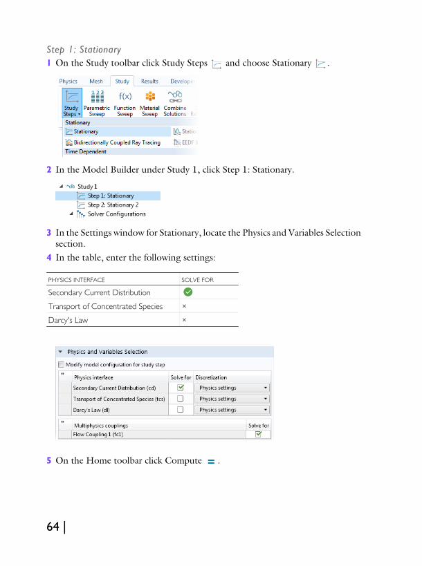
Step 1: Stationary1 On the Study toolbar click Study Steps and choose Stationary .

2 In the Model Builder under Study 1, click Step 1: Stationary.

3 In the Settings window for Stationary, locate the Physics and Variables Selection section.

4 In the table, enter the following settings:

5 On the Home toolbar click Compute .

PHYSICS INTERFACE SOLVE FOR

Secondary Current Distribution

Transport of Concentrated Species ×

Darcy's Law ×

64 |

Results for the Concentration Dependent Problem

The overpotential plot should now look like this:

Your current density plot should now look like this:

| 65

Isosurface 1Create a plot of the mass fraction of oxygen in the gas phase as follows:1 On the Home toolbar click Add Plot Group and choose 3D Plot

Group .2 On the 3D Plot Group 7 toolbar click Isosurface .3 In the Settings window for Isosurface, click Replace Expression in the

upper-right corner of the Expression section and choose Mass fraction (w_o2).

4 Locate the Levels section. In the Total levels text field, type 10.5 On the 3D Plot Group toolbar click Plot .

The oxygen mass fraction plot should now look like this:

66 |

6 Right-click 3D Plot Group 7 and choose Rename.7 Go to the Rename 3D Plot Group dialog box and type Oxygen Mass Fraction in the New name text field. Click OK.

Slice 1Create a slice plot of the gas velocity magnitude as follows:1 On the Home toolbar click Add Plot Group . Choose 3D Plot Group .2 On the 3D Plot Group 8 toolbar click Slice .3 In the Settings window for Slice click Replace Expression and choose

Darcy’s velocity magnitude (dl.U). 4 Right-click Slice 1 and choose Duplicate .5 In the Settings window for Slice locate the Plane Data section. From the Plane

list, choose zx-planes.6 Click to expand the Inherit style section. From the Plot list, choose Slice 1.7 On the 3D Plot Group toolbar click Plot . The velocity plot should look like this:

8 Click 3D Plot Group 8 and press F2. 9 Go to the Rename 3D Plot Group dialog box and type Velocity Magnitude

in the New name text field. Click OK.

| 67

68 |