introduction to symbolic computationhomepages.math.uic.edu/~jan/mcs320/mcs320.pdf · this document...
TRANSCRIPT
Introduction to Symbolic ComputationRelease 0.2.6
Jan Verschelde
Apr 18, 2017

Contents
1 Preface 1
2 Part I: first steps with Sage 32.1 Lecture 1: Welcome to MCS 320 . . . . . . . . . . . . . . . . . . . . . . . . . . . . . . . . . . . . 3
2.1.1 What is Computer Algebra? . . . . . . . . . . . . . . . . . . . . . . . . . . . . . . . . . . 32.1.2 What is Sage? . . . . . . . . . . . . . . . . . . . . . . . . . . . . . . . . . . . . . . . . . . 42.1.3 Running Sage . . . . . . . . . . . . . . . . . . . . . . . . . . . . . . . . . . . . . . . . . . 42.1.4 Which systems in Sage are used? . . . . . . . . . . . . . . . . . . . . . . . . . . . . . . . . 52.1.5 Assignments . . . . . . . . . . . . . . . . . . . . . . . . . . . . . . . . . . . . . . . . . . 5
2.2 Lecture 2: Sage as a Calculator – getting Help . . . . . . . . . . . . . . . . . . . . . . . . . . . . . 52.2.1 Getting Started . . . . . . . . . . . . . . . . . . . . . . . . . . . . . . . . . . . . . . . . . 62.2.2 Getting Help . . . . . . . . . . . . . . . . . . . . . . . . . . . . . . . . . . . . . . . . . . 72.2.3 The Packages in Sage . . . . . . . . . . . . . . . . . . . . . . . . . . . . . . . . . . . . . . 72.2.4 Assignments . . . . . . . . . . . . . . . . . . . . . . . . . . . . . . . . . . . . . . . . . . 8
2.3 Lecture 3: Exact and Floating-Point Numbers . . . . . . . . . . . . . . . . . . . . . . . . . . . . . . 82.3.1 Integer and Rational Numbers . . . . . . . . . . . . . . . . . . . . . . . . . . . . . . . . . 82.3.2 Floating-Point Numbers . . . . . . . . . . . . . . . . . . . . . . . . . . . . . . . . . . . . 92.3.3 Assignments . . . . . . . . . . . . . . . . . . . . . . . . . . . . . . . . . . . . . . . . . . 10
2.4 Lecture 4: Complex and Algebraic Numbers . . . . . . . . . . . . . . . . . . . . . . . . . . . . . . 112.4.1 Complex Numbers . . . . . . . . . . . . . . . . . . . . . . . . . . . . . . . . . . . . . . . 112.4.2 Algebraic Numbers . . . . . . . . . . . . . . . . . . . . . . . . . . . . . . . . . . . . . . . 122.4.3 Assignments . . . . . . . . . . . . . . . . . . . . . . . . . . . . . . . . . . . . . . . . . . 13
2.5 Lecture 5: Symbols, Variables, and References . . . . . . . . . . . . . . . . . . . . . . . . . . . . . 142.5.1 Expressions and Names . . . . . . . . . . . . . . . . . . . . . . . . . . . . . . . . . . . . . 142.5.2 Verification of Solutions . . . . . . . . . . . . . . . . . . . . . . . . . . . . . . . . . . . . 142.5.3 Evaluation of Expressions . . . . . . . . . . . . . . . . . . . . . . . . . . . . . . . . . . . 152.5.4 References and Shared Values . . . . . . . . . . . . . . . . . . . . . . . . . . . . . . . . . 162.5.5 Assignments . . . . . . . . . . . . . . . . . . . . . . . . . . . . . . . . . . . . . . . . . . 17
2.6 Lecture 6: Data Types and Data Structures . . . . . . . . . . . . . . . . . . . . . . . . . . . . . . . 172.6.1 Coercing to the Basic Number Types . . . . . . . . . . . . . . . . . . . . . . . . . . . . . . 172.6.2 Components of Expressions . . . . . . . . . . . . . . . . . . . . . . . . . . . . . . . . . . 182.6.3 Storing Data with Functions . . . . . . . . . . . . . . . . . . . . . . . . . . . . . . . . . . 182.6.4 Assignments . . . . . . . . . . . . . . . . . . . . . . . . . . . . . . . . . . . . . . . . . . 20
2.7 Lecture 7: Evaluation and Execution . . . . . . . . . . . . . . . . . . . . . . . . . . . . . . . . . . 202.7.1 Addition and Multiplication Tables . . . . . . . . . . . . . . . . . . . . . . . . . . . . . . . 202.7.2 Expression Trees . . . . . . . . . . . . . . . . . . . . . . . . . . . . . . . . . . . . . . . . 22
i
2.7.3 Assignments . . . . . . . . . . . . . . . . . . . . . . . . . . . . . . . . . . . . . . . . . . 242.8 Lecture 8: Input/Output Formats – Saving Data . . . . . . . . . . . . . . . . . . . . . . . . . . . . . 24
2.8.1 Files in Python . . . . . . . . . . . . . . . . . . . . . . . . . . . . . . . . . . . . . . . . . 242.8.2 Saving and Loading Sage Objects . . . . . . . . . . . . . . . . . . . . . . . . . . . . . . . 252.8.3 Pickling Objects . . . . . . . . . . . . . . . . . . . . . . . . . . . . . . . . . . . . . . . . . 252.8.4 Assignments . . . . . . . . . . . . . . . . . . . . . . . . . . . . . . . . . . . . . . . . . . 27
2.9 Lecture 9: Code Generation with Cython . . . . . . . . . . . . . . . . . . . . . . . . . . . . . . . . 272.9.1 A Motivating Example . . . . . . . . . . . . . . . . . . . . . . . . . . . . . . . . . . . . . 272.9.2 Executing in Pure Python . . . . . . . . . . . . . . . . . . . . . . . . . . . . . . . . . . . . 282.9.3 Vectorization with numpy . . . . . . . . . . . . . . . . . . . . . . . . . . . . . . . . . . . . 282.9.4 Cython code . . . . . . . . . . . . . . . . . . . . . . . . . . . . . . . . . . . . . . . . . . . 292.9.5 Assignments . . . . . . . . . . . . . . . . . . . . . . . . . . . . . . . . . . . . . . . . . . 30
3 Part II: polynomials and expressions 313.1 Lecture 10: univariate and multivariate polynomials . . . . . . . . . . . . . . . . . . . . . . . . . . 31
3.1.1 polynomials as expressions . . . . . . . . . . . . . . . . . . . . . . . . . . . . . . . . . . . 313.1.2 univariate polynomials . . . . . . . . . . . . . . . . . . . . . . . . . . . . . . . . . . . . . 323.1.3 multivariate polynomials . . . . . . . . . . . . . . . . . . . . . . . . . . . . . . . . . . . . 343.1.4 Assignments . . . . . . . . . . . . . . . . . . . . . . . . . . . . . . . . . . . . . . . . . . 34
3.2 Lecture 11: rational functions and conversions . . . . . . . . . . . . . . . . . . . . . . . . . . . . . 353.2.1 rational expressions . . . . . . . . . . . . . . . . . . . . . . . . . . . . . . . . . . . . . . . 353.2.2 conversions . . . . . . . . . . . . . . . . . . . . . . . . . . . . . . . . . . . . . . . . . . . 363.2.3 assignments . . . . . . . . . . . . . . . . . . . . . . . . . . . . . . . . . . . . . . . . . . . 37
3.3 Lecture 12: representation of expressions . . . . . . . . . . . . . . . . . . . . . . . . . . . . . . . . 373.3.1 expression trees . . . . . . . . . . . . . . . . . . . . . . . . . . . . . . . . . . . . . . . . . 373.3.2 evaluation of expressions . . . . . . . . . . . . . . . . . . . . . . . . . . . . . . . . . . . . 393.3.3 Assignments . . . . . . . . . . . . . . . . . . . . . . . . . . . . . . . . . . . . . . . . . . 39
3.4 Lecture 13: substitution, expansion, and factorization . . . . . . . . . . . . . . . . . . . . . . . . . . 393.4.1 substitution . . . . . . . . . . . . . . . . . . . . . . . . . . . . . . . . . . . . . . . . . . . 403.4.2 expansion . . . . . . . . . . . . . . . . . . . . . . . . . . . . . . . . . . . . . . . . . . . . 413.4.3 factorization . . . . . . . . . . . . . . . . . . . . . . . . . . . . . . . . . . . . . . . . . . . 423.4.4 assignments . . . . . . . . . . . . . . . . . . . . . . . . . . . . . . . . . . . . . . . . . . . 42
3.5 Lecture 14: normalizing expressions . . . . . . . . . . . . . . . . . . . . . . . . . . . . . . . . . . . 423.5.1 normal and canonical form . . . . . . . . . . . . . . . . . . . . . . . . . . . . . . . . . . . 423.5.2 rewriting multivariate polynomials . . . . . . . . . . . . . . . . . . . . . . . . . . . . . . . 433.5.3 a numerical test on equality . . . . . . . . . . . . . . . . . . . . . . . . . . . . . . . . . . . 443.5.4 assignments . . . . . . . . . . . . . . . . . . . . . . . . . . . . . . . . . . . . . . . . . . . 44
3.6 Lecture 15: review of the first 14 lectures . . . . . . . . . . . . . . . . . . . . . . . . . . . . . . . . 443.7 Lecture 16: first midterm exam . . . . . . . . . . . . . . . . . . . . . . . . . . . . . . . . . . . . . 45
4 Part III: Calculus 474.1 Lecture 17: defining mathematical functions . . . . . . . . . . . . . . . . . . . . . . . . . . . . . . 47
4.1.1 functions in Sage and in Python . . . . . . . . . . . . . . . . . . . . . . . . . . . . . . . . 474.1.2 step functions . . . . . . . . . . . . . . . . . . . . . . . . . . . . . . . . . . . . . . . . . . 484.1.3 combining functions . . . . . . . . . . . . . . . . . . . . . . . . . . . . . . . . . . . . . . 504.1.4 assignments . . . . . . . . . . . . . . . . . . . . . . . . . . . . . . . . . . . . . . . . . . . 50
4.2 Lecture 18: recursive functions . . . . . . . . . . . . . . . . . . . . . . . . . . . . . . . . . . . . . 504.2.1 memoization in Python . . . . . . . . . . . . . . . . . . . . . . . . . . . . . . . . . . . . . 504.2.2 memoization in Sage . . . . . . . . . . . . . . . . . . . . . . . . . . . . . . . . . . . . . . 524.2.3 assignments . . . . . . . . . . . . . . . . . . . . . . . . . . . . . . . . . . . . . . . . . . . 53
4.3 Lecture 19: working with functions . . . . . . . . . . . . . . . . . . . . . . . . . . . . . . . . . . . 544.3.1 list comprehensions . . . . . . . . . . . . . . . . . . . . . . . . . . . . . . . . . . . . . . . 544.3.2 composing functions . . . . . . . . . . . . . . . . . . . . . . . . . . . . . . . . . . . . . . 554.3.3 functions returning functions . . . . . . . . . . . . . . . . . . . . . . . . . . . . . . . . . . 57
ii

4.3.4 assignments . . . . . . . . . . . . . . . . . . . . . . . . . . . . . . . . . . . . . . . . . . . 584.4 Lecture 20: symbolic and numeric differentiation . . . . . . . . . . . . . . . . . . . . . . . . . . . . 59
4.4.1 symbolic differentiation . . . . . . . . . . . . . . . . . . . . . . . . . . . . . . . . . . . . . 594.4.2 numerical differentiation . . . . . . . . . . . . . . . . . . . . . . . . . . . . . . . . . . . . 604.4.3 implicit differentiation . . . . . . . . . . . . . . . . . . . . . . . . . . . . . . . . . . . . . 604.4.4 assignments . . . . . . . . . . . . . . . . . . . . . . . . . . . . . . . . . . . . . . . . . . . 61
4.5 Lecture 21: integration and summation . . . . . . . . . . . . . . . . . . . . . . . . . . . . . . . . . 614.5.1 indefinite and definite integrals . . . . . . . . . . . . . . . . . . . . . . . . . . . . . . . . . 614.5.2 assisting the integrator . . . . . . . . . . . . . . . . . . . . . . . . . . . . . . . . . . . . . 624.5.3 symbolic summation . . . . . . . . . . . . . . . . . . . . . . . . . . . . . . . . . . . . . . 634.5.4 assignments . . . . . . . . . . . . . . . . . . . . . . . . . . . . . . . . . . . . . . . . . . . 64
4.6 Lecture 22: series, approximations, and limits . . . . . . . . . . . . . . . . . . . . . . . . . . . . . . 644.6.1 Taylor series . . . . . . . . . . . . . . . . . . . . . . . . . . . . . . . . . . . . . . . . . . . 644.6.2 Taylor series in SymPy . . . . . . . . . . . . . . . . . . . . . . . . . . . . . . . . . . . . . 654.6.3 power series . . . . . . . . . . . . . . . . . . . . . . . . . . . . . . . . . . . . . . . . . . . 664.6.4 approximations . . . . . . . . . . . . . . . . . . . . . . . . . . . . . . . . . . . . . . . . . 674.6.5 limits . . . . . . . . . . . . . . . . . . . . . . . . . . . . . . . . . . . . . . . . . . . . . . 674.6.6 assignments . . . . . . . . . . . . . . . . . . . . . . . . . . . . . . . . . . . . . . . . . . . 67
4.7 Lecture 23: symbolic-numeric computation . . . . . . . . . . . . . . . . . . . . . . . . . . . . . . . 684.7.1 interval arithmetic . . . . . . . . . . . . . . . . . . . . . . . . . . . . . . . . . . . . . . . . 684.7.2 constrained optimization . . . . . . . . . . . . . . . . . . . . . . . . . . . . . . . . . . . . 694.7.3 assignments . . . . . . . . . . . . . . . . . . . . . . . . . . . . . . . . . . . . . . . . . . . 70
5 Part IV: plotting and solving equations 715.1 Lecture 24: two dimensional plots . . . . . . . . . . . . . . . . . . . . . . . . . . . . . . . . . . . . 71
5.1.1 plotting formulas and functions . . . . . . . . . . . . . . . . . . . . . . . . . . . . . . . . . 715.1.2 curves in the plane . . . . . . . . . . . . . . . . . . . . . . . . . . . . . . . . . . . . . . . 725.1.3 plotting matrices . . . . . . . . . . . . . . . . . . . . . . . . . . . . . . . . . . . . . . . . 735.1.4 assignments . . . . . . . . . . . . . . . . . . . . . . . . . . . . . . . . . . . . . . . . . . . 73
5.2 Lecture 25: plotting in three dimensions and beyond . . . . . . . . . . . . . . . . . . . . . . . . . . 745.2.1 surface plots . . . . . . . . . . . . . . . . . . . . . . . . . . . . . . . . . . . . . . . . . . . 745.2.2 space curves . . . . . . . . . . . . . . . . . . . . . . . . . . . . . . . . . . . . . . . . . . . 755.2.3 colormaps . . . . . . . . . . . . . . . . . . . . . . . . . . . . . . . . . . . . . . . . . . . . 755.2.4 assignments . . . . . . . . . . . . . . . . . . . . . . . . . . . . . . . . . . . . . . . . . . . 77
5.3 Lecture 26: animations . . . . . . . . . . . . . . . . . . . . . . . . . . . . . . . . . . . . . . . . . . 785.3.1 animating plots . . . . . . . . . . . . . . . . . . . . . . . . . . . . . . . . . . . . . . . . . 785.3.2 animating curves . . . . . . . . . . . . . . . . . . . . . . . . . . . . . . . . . . . . . . . . 785.3.3 animating surfaces . . . . . . . . . . . . . . . . . . . . . . . . . . . . . . . . . . . . . . . 795.3.4 assignments . . . . . . . . . . . . . . . . . . . . . . . . . . . . . . . . . . . . . . . . . . . 79
5.4 Lecture 27: solving equations . . . . . . . . . . . . . . . . . . . . . . . . . . . . . . . . . . . . . . 795.4.1 polynomials in one variable . . . . . . . . . . . . . . . . . . . . . . . . . . . . . . . . . . . 795.4.2 solving systems of polynomial equations . . . . . . . . . . . . . . . . . . . . . . . . . . . . 805.4.3 Groebner bases . . . . . . . . . . . . . . . . . . . . . . . . . . . . . . . . . . . . . . . . . 825.4.4 assignments . . . . . . . . . . . . . . . . . . . . . . . . . . . . . . . . . . . . . . . . . . . 82
5.5 Lecture 28: linear algebra . . . . . . . . . . . . . . . . . . . . . . . . . . . . . . . . . . . . . . . . 835.5.1 matrices and linear systems . . . . . . . . . . . . . . . . . . . . . . . . . . . . . . . . . . . 835.5.2 matrices over fields . . . . . . . . . . . . . . . . . . . . . . . . . . . . . . . . . . . . . . . 845.5.3 matrices over rings . . . . . . . . . . . . . . . . . . . . . . . . . . . . . . . . . . . . . . . 855.5.4 resultants . . . . . . . . . . . . . . . . . . . . . . . . . . . . . . . . . . . . . . . . . . . . 865.5.5 assignments . . . . . . . . . . . . . . . . . . . . . . . . . . . . . . . . . . . . . . . . . . . 87
5.6 Lecture 29: solving differential equations . . . . . . . . . . . . . . . . . . . . . . . . . . . . . . . . 875.6.1 the pendulum problem . . . . . . . . . . . . . . . . . . . . . . . . . . . . . . . . . . . . . 875.6.2 heat diffusion . . . . . . . . . . . . . . . . . . . . . . . . . . . . . . . . . . . . . . . . . . 885.6.3 assignments . . . . . . . . . . . . . . . . . . . . . . . . . . . . . . . . . . . . . . . . . . . 88
iii

5.7 Lecture 30: Polyhedra and Linear Programming . . . . . . . . . . . . . . . . . . . . . . . . . . . . 895.7.1 polyhedra . . . . . . . . . . . . . . . . . . . . . . . . . . . . . . . . . . . . . . . . . . . . 895.7.2 linear programming . . . . . . . . . . . . . . . . . . . . . . . . . . . . . . . . . . . . . . . 895.7.3 unconstrained minimization . . . . . . . . . . . . . . . . . . . . . . . . . . . . . . . . . . 905.7.4 assignments . . . . . . . . . . . . . . . . . . . . . . . . . . . . . . . . . . . . . . . . . . . 90
5.8 Lecture 31: review of lectures 17 to 30 . . . . . . . . . . . . . . . . . . . . . . . . . . . . . . . . . 915.9 Lecture 32: second midterm exam . . . . . . . . . . . . . . . . . . . . . . . . . . . . . . . . . . . . 92
6 Part Five : advanced Sage 936.1 Lecture 33: building interactive web pages . . . . . . . . . . . . . . . . . . . . . . . . . . . . . . . 93
6.1.1 drawing tangent lines to a curve . . . . . . . . . . . . . . . . . . . . . . . . . . . . . . . . 936.1.2 making the web page . . . . . . . . . . . . . . . . . . . . . . . . . . . . . . . . . . . . . . 946.1.3 drop down menu . . . . . . . . . . . . . . . . . . . . . . . . . . . . . . . . . . . . . . . . 946.1.4 assignments . . . . . . . . . . . . . . . . . . . . . . . . . . . . . . . . . . . . . . . . . . . 95
6.2 Lecture 34: an application of interact . . . . . . . . . . . . . . . . . . . . . . . . . . . . . . . . . . 956.2.1 turning a crank . . . . . . . . . . . . . . . . . . . . . . . . . . . . . . . . . . . . . . . . . 956.2.2 computing coordinates of the connector point . . . . . . . . . . . . . . . . . . . . . . . . . 956.2.3 adding the coupler and fourth bar . . . . . . . . . . . . . . . . . . . . . . . . . . . . . . . . 976.2.4 deploying the interactive web page . . . . . . . . . . . . . . . . . . . . . . . . . . . . . . . 976.2.5 assignments . . . . . . . . . . . . . . . . . . . . . . . . . . . . . . . . . . . . . . . . . . . 97
6.3 Lecture 35: symbolic computation with sympy . . . . . . . . . . . . . . . . . . . . . . . . . . . . . 986.3.1 sympy outside Sage . . . . . . . . . . . . . . . . . . . . . . . . . . . . . . . . . . . . . . . 986.3.2 sympy inside Sage . . . . . . . . . . . . . . . . . . . . . . . . . . . . . . . . . . . . . . . 986.3.3 assignment . . . . . . . . . . . . . . . . . . . . . . . . . . . . . . . . . . . . . . . . . . . 99
6.4 Lecture 36: numerical computation with numpy and scipy . . . . . . . . . . . . . . . . . . . . . . . 996.4.1 numpy . . . . . . . . . . . . . . . . . . . . . . . . . . . . . . . . . . . . . . . . . . . . . . 996.4.2 scipy . . . . . . . . . . . . . . . . . . . . . . . . . . . . . . . . . . . . . . . . . . . . . . . 1006.4.3 assignments . . . . . . . . . . . . . . . . . . . . . . . . . . . . . . . . . . . . . . . . . . . 102
6.5 Lecture 37: Maxima, a component in Sage . . . . . . . . . . . . . . . . . . . . . . . . . . . . . . . 1026.5.1 maxima . . . . . . . . . . . . . . . . . . . . . . . . . . . . . . . . . . . . . . . . . . . . . 102
6.6 Lecture 38: computational group theory with GAP . . . . . . . . . . . . . . . . . . . . . . . . . . . 1046.6.1 permutation groups . . . . . . . . . . . . . . . . . . . . . . . . . . . . . . . . . . . . . . . 1046.6.2 Rubik’s cube . . . . . . . . . . . . . . . . . . . . . . . . . . . . . . . . . . . . . . . . . . 1056.6.3 assignments . . . . . . . . . . . . . . . . . . . . . . . . . . . . . . . . . . . . . . . . . . . 106
6.7 Lecture 39: higher arithmetic with Pari/GP . . . . . . . . . . . . . . . . . . . . . . . . . . . . . . . 1076.7.1 calculating with GP in Sage . . . . . . . . . . . . . . . . . . . . . . . . . . . . . . . . . . 1076.7.2 the Cauchy integral formula . . . . . . . . . . . . . . . . . . . . . . . . . . . . . . . . . . 1086.7.3 expansions and series . . . . . . . . . . . . . . . . . . . . . . . . . . . . . . . . . . . . . . 1086.7.4 integer relation detection . . . . . . . . . . . . . . . . . . . . . . . . . . . . . . . . . . . . 1096.7.5 assignments . . . . . . . . . . . . . . . . . . . . . . . . . . . . . . . . . . . . . . . . . . . 109
6.8 Lecture 40: computing with polynomials in Singular . . . . . . . . . . . . . . . . . . . . . . . . . . 1096.8.1 polynomials . . . . . . . . . . . . . . . . . . . . . . . . . . . . . . . . . . . . . . . . . . . 1106.8.2 reducing polynomials with a Groebner basis . . . . . . . . . . . . . . . . . . . . . . . . . . 1116.8.3 assignments . . . . . . . . . . . . . . . . . . . . . . . . . . . . . . . . . . . . . . . . . . . 112
6.9 Lecture 41: statistical computing with R . . . . . . . . . . . . . . . . . . . . . . . . . . . . . . . . . 1126.9.1 computations with R . . . . . . . . . . . . . . . . . . . . . . . . . . . . . . . . . . . . . . 1126.9.2 plotting data . . . . . . . . . . . . . . . . . . . . . . . . . . . . . . . . . . . . . . . . . . . 1136.9.3 fitting linear models . . . . . . . . . . . . . . . . . . . . . . . . . . . . . . . . . . . . . . . 113
7 Indices and tables 115
iv

CHAPTER 1
Preface
This document contains the lecture notes for the course MCS 320, introduction to symbolic computation, at theUniversity of Illinois at Chicago. The course was inspired by the book of A. Heck, introduction to Maple, the secondedition, published by Springer in 1996. From 2001 till 2014, the course was offered, using Maple, about once everyacademic year. Since Spring 2015, Maple was replaced by Sage.
1

Introduction to Symbolic Computation, Release 0.2.6
2 Chapter 1. Preface
CHAPTER 2
Part I: first steps with Sage
The first part of the course consists of the first 9 lectures during first three weeks of classes. One strength of computeralgebra is the wide range of number types and arithmetic that go beyond what is offered by the computer arithmetic.In addition to exact rational and arbitrary multiprecision floating-point arithmetic, we cover complex and algebraicnumbers. For the latter, we introduce the basics of expressions, and in particular polynomials with coefficients overany number field.
2.1 Lecture 1: Welcome to MCS 320
In this first lecture we define computer algebra and sketch the organization of the course. The most important aspectof this lecture is to get started with the notebook interface in Sage.
We can run Sage in a terminal window, in the cell server, in a notebook, or in the cloud. Our running computationinvolves the symbol pi which Sage recognizes as the mathematical constant 𝜋. The lecture ends with finding outwhich system performs a particular calculation.
2.1.1 What is Computer Algebra?
Computer Algebra is the discipline that studies the algorithms for Symbolic Computation. In Symbolic Computation,one computes with symbols, rather than with numbers. In this course we are mostly concerned with the practicalaspects of Symbolic Computation, in particular its implementation and its application to solve practical mathematicalproblems.
The lecture notes are organized in four parts:
1. First steps with Sage
2. Polynomials and rational expressions
3. Functions and Calculus
4. More Advanced Sage
5. Some Components of Sage
3
Introduction to Symbolic Computation, Release 0.2.6
2.1.2 What is Sage?
Nowadays we write Sage as a name, but originally SAGE was short for Software for Algebra, Geometry, and Experi-mentation. Below are some important points about Sage:
• Sage is released as free and open source software under the terms of the GNU General Public License.
• As scripting language, Sage uses Python. Sage has a large, active developers community.
• By design, Sage does not reinvent the wheel, but bundles various powerful free and open source mathemati-cal software systems, such as GAP, Maxima, R, Singular, sympy, numpy, scipy, etc. This design principle isvisualized in Fig. 2.1.
Fig. 2.1: The motto of Sage: building the car instead of reinventing the wheel.
• Try it without installing, via the Sage Cell Server: https://sagecell.sagemath.org/, or with the SageMathCloud:https://cloud.sagemath.com.
2.1.3 Running Sage
There are two main modes to run Sage:
• In a terminal window, which is similar as using the command line interface to interactive software systems. Thisworks fine for short calculations, when the right commands are knows in advance.
• The notebook interface runs in a web browser. The help gives direct access to the reference manual and otherdocumentation. The notebook interface is natural with cloud computing.
A terminal session with Sage
sage: pipisage: sin(pi)0sage: '%.14e' % pi'3.14159265358979e+00'sage: type(_)<type 'str'>sage: type(pi)<type 'sage.symbolic.expression.Expression'>sage: p = plot(sin,(-pi,+pi))sage: p
4 Chapter 2. Part I: first steps with Sage

Introduction to Symbolic Computation, Release 0.2.6
For a more interesting plot, consider the sine function with a decaying amplitude, as defined byexp(-x^2)*sin(8*x).
As a computer algebra system, Sage is mainly for symbolic computation. For its numerical computations, we are notlimited to the hardware machine arithmetic. For example, to see the decimal exponsion of 𝜋 with 20 decimal places:
sage: pi20 = pi.n(digits=20)sage: print pi203.1415926535897932385sage: print sin(pi20)6.5640070857470010853e-22sage: print type(pi20)<type 'sage.rings.real_mpfr.RealNumber'>
Unlike the exact value for 𝜋, the value of sin(pi20) is no longer zero.
In the Sage Cell Server to plot the sine function, we can enter:
var('x')plot(sin(x), (-pi, pi)).show()
When running the notebook interface, we can document our computations with text that follows the # symbol.
2.1.4 Which systems in Sage are used?
Sage is built out of several systems. If you are curious to see which software package executed your calculation, youcould proceed as follows:
sage: from sage.misc.citation import get_systemssage: get_systems('Rational(0.75)')['MPFR']sage: get_systems('RealField(10)(pi)')['MPFR', 'ginac']sage: import sage.misc.citationsage: help(sage.misc.citation)sage: print sage.misc.citation.systems.keys()
2.1.5 Assignments
1. Go to http://www.sagemath.org/tour.html and take the Feature tour.
After taking this tour, write a couple of sentences (one paragraph long) about what interests you most.
2. Create an account on https://cloud.sagemath.com, the SageMathCloud, and make a notebook with calculationsfrom this lecture.
3. If there is sufficient disk space available on your home computer or laptop, consider installing Sage from source.On Linux systems, you should not do this installation as root, but as an ordinary user.
4. Which system executes the statement pi.n(digits=20)?
2.2 Lecture 2: Sage as a Calculator – getting Help
In this lecture we show how to use the Sage notebook as a calculator and explore the extensive help facilities.
2.2. Lecture 2: Sage as a Calculator – getting Help 5

Introduction to Symbolic Computation, Release 0.2.6
If we compute with arbitrary multiprecision, then we must raise the precision of the field to compute the roundingerrors correctly. We illustrate this with the computation of a numerical approximation to 𝜋, accurate up to 30 decimalplaces. We explore the help system of Sage, priming the continued fractions of the next lecture.
2.2.1 Getting Started
We run the notebook in multicell mode. In the command line interface, the commands are executed in sequence, inthe notebook interface, we can execute commands out of order.
We enter mathematical expressions in a cell. The expressions are executed by clicking on the evaluate button whichappears below each cell. For example:
34^34
With the underscore we get the result from the previous computation. Note that previous refers to time, not location.To experience this, we add in the next cell the underscore, and then in the following cell:
2*3
When we evaluate we see the result 6 appear and when we evaluate the cell with the underscore that is located abovethe cell 2*3, then we will see the result change from the value of 34^34 into 6. Consider the next cell with content
pipi - _
Repeatedly clicking on the evaluate button will give different results each time. Can you explain the differences?
At the command line interface: (but not in the notebook interface) we can use double and triple underscores:
sage: 22sage: 33sage: 44sage: ___2sage: ___3sage: ___4sage: __3sage: _3
Consider the computation of the difference between pi and a 30 digit numerical approximation for pi. The shortestway to obtain this is via pi.n(digits=30). Another way is via numerical_approx as illustrated below:
numerical_approx(pi,digits=30)
But often we want to compute with a precision of 30 decimal places. Then we compute with a RealField ofprescribed precision. For a 30-digit approximation of pi we then type in a cell:
R = RealField(30*log(10,2))pi30 = R(pi)
6 Chapter 2. Part I: first steps with Sage
Introduction to Symbolic Computation, Release 0.2.6
strpi30 = str(pi30)print '%d-digit approximation for pi : %s' % (len(strpi30),strpi30)
With log(10,2) we compute the binary logarithm of 10, because the argument of RealField is expressed in bits.After the creation of R, we convert the symbol for the mathematical constant pi into a 30-digit approximation for pi.This approximation is stored in the variable pi30. The conversion to the string representation str(pi30) is usedto check that indeed we do have 30 decimal places, as in confirmed by the output produced by the cell.
As simple computation of the difference between pi and pi30 can be done as
R(pi - pi30)
which returns 0.00000000000000000000000000000
The problem with the previous computation is that the precision of the RealField was not large enough. To make thedifference with 40 decimal places:
RealField(40*log(10,2))(pi-pi30)
yields 1.69568553528388823010177990083205496387e-31. Thus we verified that pi30 has the desired accuracy of30 decimal places.
Next we illustrate the difference between precision and accuracy:
pi40 = RealField(40*log(10,2))(pi30)
we have made a variable pi40 with a working precision of 40 decimal places. But because it takes the value of pi30,the accuracy of pi40 is no more than 30 decimal places.
2.2.2 Getting Help
To see the documentation for a specific command, in a cell we can type
help(RealField)
To look for a specific topic, we can use the search_doc as illustrated below:
search_doc("continued fraction")
In the SageMath Cloud, the user gets redirected to the extensive online documentation.
2.2.3 The Packages in Sage
There are many packages in Sage where we can find pi:
print type(pi)print type(math.pi)import sympyprint type(sympy.pi)import numpyprint type(numpy.pi)
The second and fourth type is the ordinary float whereas the first and third type are symbolic.
To work with the pi as defined by sympy:
2.2. Lecture 2: Sage as a Calculator – getting Help 7

Introduction to Symbolic Computation, Release 0.2.6
from sympy import pi as sympypiprint sin(sympypi)print sympypi.evalf(30)
The first number we see is 0 followed by a 30-digit approximation for pi.
2.2.4 Assignments
In assignments where you are asked to explain, please formulate your answers with complete sentences.
1. Explain the differences between pi and Pi in Sage. Illustrate the differences with the appropriate commands.
2. Verify that Sage knows that the exponential of the natural logarithm of 2 equals 2.
3. The mathematical constant e is just as pi a transcendental number. Show that Sage knows the constant e bytaking its natural logarithm. Calculate a 30-digit approximation for e. Verify the accuracy of this approximationby calculating its difference with the exact value.
4. Consider the following sequence of commands:
R = RealField(30*log(10,2))print tan(R(pi/2))print R(tan(pi/2))
Why do these two commands give different answers? Which of the two commands gives the correct answer?Also compare R(tan(pi)) with tan(R(Pi)) and explain the differences.
5. The decomposition of 2015 as a product of prime numbers is 5 * 13 * 31. Use the help system of Sage tofind the command to compute the factorization of a natural number.
2.3 Lecture 3: Exact and Floating-Point Numbers
The capability to compute exactly and in high precision is one of the main features of computer algebra. In this lecturewe illustrate how to compute exactly with integer and rational numbers, and to compute with multiprecision arithmetic.
We can approximate a transcendental number such as 𝜋 as a floating-point number up to any number of decimalplaces. Instead of a floating-point approximation, we may approximate with a continued fraction expansion. In Sagewe can compute continued fractions up to a certain number of terms or up to a given number of bits in the precision.The convergents of a continued fraction gives us a sequence of increasingly more accurate rational approximationsfor 𝜋. We cover machine precision. Irrational and algebraic numbers are defined. We introduce the reverse operationto computing an approximation of an irrational number. Given an approximation for a number and a tolerance, wemay find the smallest polynomial that has this number as a root. For example, with sympy we compute
√2 from an
approximation for the√2, as
√2 is a solution of 𝑥2 − 2.
2.3.1 Integer and Rational Numbers
The division of two integer numbers gives a rational number. Selecting its numerator and denominator is straightfor-ward:
a = 3/4print type(a)print numerator(a), denominator(a)
8 Chapter 2. Part I: first steps with Sage

Introduction to Symbolic Computation, Release 0.2.6
Any irrational or transcendental can be approximated with continued fractions. A continued fraction is defined by alist of natural numbers, which are called convergents. For example:
x = sqrt(2)c = continued_fraction(x)print c
which prints [1; 2, 2, 2, 2, 2, 2, 2, 2, 2, 2, 2, 2, 2, 2, 2, 2, 2, 2, 2, ...] Thelist of convergents defines the continued fraction. For example, the list [1, 2, 2, 2, 2] defines
1 +1
2 + 12+ 1
2+ 12
We may verify that the above fraction approximates√2 up to 3 correct decimal places:
f = 1 + 1/(2 + 1/(2 + 1/(2 + 1/2)))print fprint float(f), float(x)print [convergents(c)[k] for k in range(5)]
Each convergent is a rational approximation. The last command is a list comprehension and prints [1, 3/2, 7/5,17/12, 41/29] which contains a list of increasingly more accurate approximations converging to
√2.
The quickest way to get a rational approximation for the square root of 2, accurate to 2 decimal places, goes as follows
sqrt(2).n(digits=2).exact_rational()
With a list comprehension, we can then compute the sequence of increasingly more accurate rational approximationsfor sqrt(2).
[sqrt(2).n(digits=k).exact_rational() for k in range(2,10)]
Note that this sequence is different from the convergents.
2.3.2 Floating-Point Numbers
The default floating-point type is float as in Python. The machine precision is defined as the largest number we canadd to 1.0 and see a difference from 1.0. A double float has 53 bits in its fraction, a single float has a fraction of 22bits long. We can verify the machine precision calculation with the predefined constants of the numpy package.
print 'machine precision (double float) :', float(2^(-52))print 'machine precision (single float) :', float(2^(-23))import numpyfrom numpy import finfoprint finfo(float).epsprint finfo(numpy.float32).eps
To compute with higher than double precision, we can make a RealField. Since the argument is in bits, we multiplywith the number of decimal places we want in our precision with the 2-logarithm of 10. For 50 decimals, we do
nbits = 50*log(10,2)print 'number of bits for 50 decimal places :', int(nbits)R = RealField(nbits)print '50-digit approximation of sqrt(2) =', R(x)
We will use this field to verify the accuracy of the convergents calculating in R with a list comprehension
2.3. Lecture 3: Exact and Floating-Point Numbers 9

Introduction to Symbolic Computation, Release 0.2.6
c = continued_fraction(sqrt(2))a = [convergents(c)[k] for k in range(20)]print ['%.2e' % R(sqrt(2)-p) for p in a]
The numbers are displayed in scientific format and we see the exponent gradually decreasing till -15, which indicatesthat the last convergent is accurate up to 15 decimal places.
A number as√2 is an irrational number. But it is not a transcendental number because
√2 is a root of 𝑥2 − 2 = 0
and therefore we say that√2 is an algebraic number. With the nsimplify of sympy, given an approximation for a
root, we can reconstruct the polynomial and thus find the closest exact number of the algebraic number.
asqrt2 = numerical_approx(sqrt(2),10)print asqrt2from sympy import nsimplifyprint nsimplify(asqrt2,tolerance=0.001,full=True)
The last statement prints sqrt(2), obtained from a 10-bit approximation 1.4 for√2.
2.3.3 Assignments
1. Explain the outcome of 3^4^5. In particular, what is the order of execution of the two exponentiation opera-tions?
2. Write 543 − 1 as a product of prime numbers.
3. The greatest common divisor of two integer numbers 𝑎 and 𝑏 can be written as a linear combination (with integercoefficients 𝑘 and ℓ) of 𝑎 and 𝑏: gcd(𝑎, 𝑏) = 𝑘𝑎+ ℓ𝑏.
In Sage this is achieved with the command xgcd. Look in the help page of this command to compute thecoefficients of the linear combination of the greatest common divisor of 12214 and 2012. Give the commandyou type in to find these coefficients and also give the command(s) to verify the result.
4. What is the difference in Sage between 1/3 + 1/3 + 1/3 and 1.0/3 + 1.0/3 + 1.0/3? Explain.
5. Consecutive rational approximations for 𝜋 are 3, 22/7, 333/106, 355/113, ... In this sequence, what is thenext more accurate rational approximation for 𝜋? How many decimal places are correct in this next rationalapproximation?
6. Explain the difference between 1.0 + 10−20 and 1 + 10−20. How can you make Sage return the same correctvalue of these two sums?
7. The golden ratio is defined as 𝑟 = 1+√5
2 . Give all Sage commands
(i) to compute a rational approximation for 𝑟 accurate with three decimal places;
(ii) to show that the accuracy of this approximation is indeed three decimal places;
(iii) to compute a sequence of the first ten consecutive rational approximations, where the k-th number of thesequence is accurate with k decimal places.
8. Consider r = 1.2599. Find the algebraic number that is closest to r.
9. Consider√3. Compute the first ten terms in the continued fraction expansion. Write the last element in the
corresponding list of convergents.
Compare the floating-point approximation of this rational approximation for√3 with the floating-point approx-
imation for√3. How many decimal places in the rational approximation are correct?
Give the floating-point approximation of the rational approximation for√3. Write only those decimals that are
correct.
10 Chapter 2. Part I: first steps with Sage

Introduction to Symbolic Computation, Release 0.2.6
2.4 Lecture 4: Complex and Algebraic Numbers
We have integer, rational, and irrational numbers. Among the irrational numbers, we distinguish between the algebraicand the transcendental numbers. An algebraic number is a root of a polynomial with integer coefficients. For atranscendental number, there does not exist a polynomial with integer coefficients that has that number as one of itsroots. Complex numbers are special type algebraic numbers and merit separate treatment.
Sage knows the symbol I as the imaginary unit. While we may define I as the square root of negative one, thisdefinition has its problems, as we then see when we cover algebraic numbers. A complex number is a special algebraicnumber and arises from the polynomial 𝑥2 + 1, which as no real root, or equivalently, 𝑥2 + 1 does not factor over thefield of real numbers. The outcome of the factor command on a polynomial in one variable depends on the choiceof coefficient field. We introduce finite fields, multiplication tables, and field extensions.
2.4.1 Complex Numbers
We could define the imaginary unit as the square root of -1 and we see that Sage represents sqrt(-1) with the symbol I.
print sqrt(-1)print type(I)print I^2
The I has type sage.symbolic.expression.Expression and its square evaluates to −1.
In rectangular coordinates, complex numbers have a real part and an imaginary part.
x = 2/3 + 5*I; print ' x =', x, '|x| =', abs(x)y = complex(2/3,5); print 'y =', y, '|x| =', abs(y)print 'x has type', type(x)print 'y has type', type(y)
While x is considers as an expression, the y is the complex type of Python. As an expression, the real and imaginarypart of a complex number may be any number type, whereas Python’s complex number is a tuple of two hardwarefloats.
An alternative to representing a complex number via its real and imaginary part (rectangular coordinates) is the polarrepresentation as its absolute value and an argument. We first must make sure the number belongs to the ComplexDouble Field, abbreviated by CDF.
ax = CDF(x).argument(); rx = abs(x)print ax, rx, 'x =', complex(rx*(cos(ax) + I*sin(ax)))
and we recognize the rectangular representation of x as we defined x above.
Complex numbers are introduced so every polynomial with real coefficients of degree d has d roots, counted withmultiplicities. By default, we get complex roots if we solve a polynomial equation. If we want to see the multiplicitiesof the roots, we must turn on the multiplicities flag.
var('z')solve(z^2 + 4 == 0, z)solve(z^2 - 2*z + 1 == 0, z, multiplicities=True)
Defining I as the square root of -1 has its problems, as we will try to illustrate next.
a = (-1 + I)^2; b = (1 - I)^2;
If we apply the sqrt() function to a and b we would expect to see -1 + I and 1 - I respectively. Instead weget sqrt(-2*I) in both cases. Why? Because, if we take a square root, we are solving a quadratic equation.
2.4. Lecture 4: Complex and Algebraic Numbers 11

Introduction to Symbolic Computation, Release 0.2.6
aq = z^2 - a == 0; bq = z^2 - b == 0;
The solution is ±√−2𝐼 . With the option all we get to see all square roots:
sqrt(a, all=True)
In contrast, we can also prevent evaluation, after coercing the argument of sqrt() to a symbolic ring, denoted bySR.
sqrt(SR(4), hold=True)
2.4.2 Algebraic Numbers
A square root is an algebraic number. The smallest polynomial that has an algebraic number as its root is the minimalpolynomial. The command
sqrt(2).minpoly()
returns 𝑥2 − 2 as the minimal polynomial of√2.
The outcome of the factoring of a polynomial depends on the number field.
print factor(z^2 - 1)print factor(z^2 - 2)
The first command will print (z + 1)*(z - 1) whereas the second polynomial does factor and we get z^2 - 2returned. If a polynomial does not factor over a specific number field (the default number field is the field of rationalnumbers), then we say that the polynomial is irreducible over that specific number field.
We can define a number field where c is the square root of 2, we can compute modulo the minimal polynomial ofsqrt(2), that is c^2 - 2 = 0. We use c^2 = 2 to simplify expressions in c.
K.<c> = NumberField(x^2 - 2); print Kprint c^2 - 2print c^3
The defining polynomial of the number field K is x^2 - 2. In this number field, the expression c^2 - c evaluatesto zero and c^3 simplifies to 2*c. If we now consider a polynomial ring over the number field K, then the polynomialx^2 - 2 will factor.
R.<x> = PolynomialRing(K)p = x^2 - 2factor(p)
On return we see (x - c) * (x + c).
In coding and cryptography we often work with finite fields.
k = GF(8,'c'); print ke = [a for a in k]; print e
This makes k a field of size 23 with elements
[0, c, c^2, c + 1, c^2 + c, c^2 + c + 1, c^2 + 1, 1]
In a field every element has a multiplicative inverse. We can see this in table of multiplications.
12 Chapter 2. Part I: first steps with Sage

Introduction to Symbolic Computation, Release 0.2.6
for x in e: [x*y for y in e]
The multiplication table is
[0, 0, 0, 0, 0, 0, 0, 0][0, c^2, c + 1, c^2 + c, c^2 + c + 1, c^2 + 1, 1, c][0, c + 1, c^2 + c, c^2 + c + 1, c^2 + 1, 1, c, c^2][0, c^2 + c, c^2 + c + 1, c^2 + 1, 1, c, c^2, c + 1][0, c^2 + c + 1, c^2 + 1, 1, c, c^2, c + 1, c^2 + c][0, c^2 + 1, 1, c, c^2, c + 1, c^2 + c, c^2 + c + 1][0, 1, c, c^2, c + 1, c^2 + c, c^2 + c + 1, c^2 + 1][0, c, c^2, c + 1, c^2 + c, c^2 + c + 1, c^2 + 1, 1]
Observe that, except for the first row, there is 1 in every row. Except for the first column, there is 1 in every column.To verify, let us look at the 1 in the second row.
print e[1], '* (', e[-2], ') =', e[1]*e[-2]
The output is c * ( c^2 + 1 ) = 1.
We can factor over finite fields. We make a polynomial ring with coefficients in the finite field we just constructed:
R.<x> = PolynomialRing(k)p = x^3 + x + 1factor(p)
which leads to (x + c) * (x + c^2) * (x + c^2 + c). Note that over the default field, the polynomialis irreducible.
q = z^3 + z + 1; factor(q)
To verify that the polynomial 𝑝 = 𝑥4 + 3𝑥+ 4 does not factor over the finite field of five elements, we do
R.<x> = PolynomialRing(GF(5))p = x^4 + 3*x + 4; print factor(p)
We can then extend the field of five elements with a root of 𝑝 as follows
F.<a> = GF(5).extension(p)e = [n for n in F]; print e
Because the degree of 𝑝 is four, every element in the field extension F can be expressed as a polynomial of degreethree or less, because every fourth power of 𝑎 simplifies via 𝑎4 = 2𝑎 + 1. We have five choices for every coefficientof a degree three polynomials and since we can make those choices independently, we have a field with 54 elements.Over this field extension, we have a factorization.
R.<y> = PolynomialRing(F)q = y^4 + 3*y + 4; print factor(q)
2.4.3 Assignments
1. The complex number 𝑧 in polar representation is given by the radius (absolute value) 𝑟 = 3 and angle (argument)𝜃 = 𝜋/3. Use Sage to find the exact (no floating-point) value of 𝑧 in the form 𝑎+ 𝑏𝐼 .
2. Execute solve(x^3 - 5 == 0, x) and show that all solutions of 𝑥3−5 = 0 are of the form 3√5𝑒𝐼𝜃, with
𝜃 being either 0 or ± 23𝜋.
2.4. Lecture 4: Complex and Algebraic Numbers 13

Introduction to Symbolic Computation, Release 0.2.6
3. Take the complex number 𝑧 = 1 + 𝐼 and let Sage compute√1/𝑧 and 1/
√𝑧. Are the results symbolically the
same? Are the results numerically the same? Give reasons for your answers, illustrated with the appropriateSage instructions.
4. Use Sage to show that the polynomial 𝑝 = 𝑥4 + 3𝑥 + 4 is irreducible over the finite field with 5 elements.Declare 𝑧 to be a root of 𝑝 and express 𝑧13 as a polynomial in 𝑧 of degree 4 (or less).
5. Compute all irreducible polynomials of degree 2 over a field with 3 elements.
2.5 Lecture 5: Symbols, Variables, and References
While Sage works with dynamic typing in a similar fashion as Python, sometimes we must declare variables explicitlywith var as in var('x').
Every variable in Sage has a type. We distinguish between names of variables and the objects variables refer to. Puttingquotes around a variable name prevents an evaluation and we see how this may be used to make connections betweenvariables. We cover the (partial) evaluation of expressions as needed in the verification of the solutions of a generalcubic equation.
2.5.1 Expressions and Names
Sage export mathematical constants, such as pi. We can work with pi as a variable and assign any value to pi. Forexample:
print pi, type(pi)pi = 3.14print pi, type(pi)
The first statement shows that pi is an expression. After the assignment, pi refers to the value 3.14 which is of typesage.rings.real_mpfr.RealLiteral. Did we then loose the value of pi?
With restore (we could also call the restore the unassign operation) we can get back the original value of pi.
restore('pi')print pi, type(pi)print numerical_approx(pi, digits=30)
Mind the quotes in the argument of restore, without the quotes we would take the value pi refers to. Afterexecuting the restore we see that pi is again an expression. And sure enough, we can see as many digits of pi aswe like.
The quotes are of course a general construction from Python where everything put between quotes is a string. A valuecan be stored as a string and then later evaluated with eval.
x = 3.14name = 'x'print x, name, eval(name)
2.5.2 Verification of Solutions
By default, with we solve an equation with‘‘solve‘‘ we receive a list of expressions.
14 Chapter 2. Part I: first steps with Sage

Introduction to Symbolic Computation, Release 0.2.6
var('z')equ = z**2 - 3 == 0sols = solve(equ, z); print solsprint type(sols[0])
We have the option to return a list of dictionaries.
sols = solve(equ, z, solution_dict=True); print sols
Now we see [{z: -sqrt(3)}, {z: sqrt(3)}] and sols is a list of dictionaries. As key for each dictio-nary we have the variable name and its corresponding value is the value of the solution of the equation. For example,to select the value of the first solution, using as key the variable name z, we can proceed as follows
print sols[0], type(sols[0])print sols[0][z]
The last command prints the value -sqrt(3). The dictionary is useful to substitute the value of the variable in theequation we solved, for verification purposes.
equ.substitute(sols[0])
and we see 0 == 0.
Suppose we were to assign to z. Then we can no longer access the dictionary as directly as before, because znow refers to a value, but via keys() we retrieve the unevaluated variable with the corresponding value. But thesubstitution still works.
z = 3; print 'z = ', zprint sols[0].keys(), sols[0].values()equ.substitute(sols[0])
Even though we have lost the use of z as a general variable, its former value as a solution is still contained in thedictionary of solutions sols.
How do we see the current value to which z refers to?
print eval(str(sols[0].keys()))
This will show the list [3]. Recall that lists in Python allow to work with shared references.
2.5.3 Evaluation of Expressions
We can express the roots of a polynomial of degree two with symbolic coefficients. Similar formulas exist for apolynomial of degree three. To start over, we clear all the variables in our worksheet with the reset().
reset()var('x, a, b, c')p = x^3 + a*x^2 + b*x + cs = solve(p == 0, x, solution_dict=True)print s
The formulas look complicated. Let us check a specific example. We want to verify the solution for specific valuesof the coefficients. An easy choice for the coefficients are the numbers 1.0, 2.0, 3.0 (of type float). Recall that Pythonallows for simultaneous or tuple assignment.
2.5. Lecture 5: Symbols, Variables, and References 15

Introduction to Symbolic Computation, Release 0.2.6
(a, b, c) = (1.0, 2.0, 3.0)print a, b, cprint pprint s[0]
The outcome is not what we wanted and expected. Even as we see the specific values for a, b, and c printed, thepolynomial still shows up in its original symbolic form 𝑥3 + 𝑎𝑥2 + 𝑏𝑥 + 𝑐, and so does its solution. If we were toretype the expression for the polynomial again, then the coefficients would be evaluated, but this is tedious and we donot want to retype the complicated expressions for the solutions.
How to force the evaluation of the coefficients in p and the solution without retyping the polynomial p? We canevaluate an expression.
print p(x=x,a=a,b=b,c=c)s0 = s[0][x](a=a,b=b,c=c); print s0
Now we see the polynomial x^3 + x^2 + 2.00000000000000*x + 3.00000000000000 and a numericalvalue for the solution.
We can then evaluate the expression p at s0.
print p(x=s0,a=a,b=b,c=c)
To verify whether the value of the expression at the solution will evaluate to zero, we convert to the complex floatingpoint type.
print complex(p(x=s0,a=a,b=b,c=c))
and we see that the value is close enough to the machine precision.
2.5.4 References and Shared Values
We first reset all variables with reset(). Then we make variables to share the same value.
reset()var('x, y, z')x = yy = zz = 3print x, y, z
What is printed is the sequence y z 3 which means that x refers to y, y refers to z, and z refers to 3. We can trackthose references with the eval() command. The eval() takes a string as argument. With repeated evals we canget from x to 3.
ex = eval(str(x)); print xey = eval(str(ex)); print eyprint eval(str(eval(str(x))))
The first eval shows y, the second one 3, just as the third nested application of eval.
Observe that the order of the assignments matters.
reset()var('x, y, z')z = 3y = z
16 Chapter 2. Part I: first steps with Sage

Introduction to Symbolic Computation, Release 0.2.6
x = yprint x, y, z
Because the right hand side in an assignment operation gets evaluated, all variables will receive the same value 3. Toprevent the evaluation of the right hand side, we use quotes.
reset()var('x, y, z')z = 3y = 'z'x = 'y'print x, y, z
The sequence that is printed is y, z, 3.
2.5.5 Assignments
1. Execute the statements reset(); var('a, b'); b = a; a = 2 and explain the relationships be-tween the variables a and b. Give the Sage commands and their output to illustrate your explanation.
2. Execute the statements reset(); var('x, y'); x = 3 in a cell. What is the next statement so printx, y shows 3, x as y refers to x, as x refers to 3.
2.6 Lecture 6: Data Types and Data Structures
Every object in Sage has a type. The type of an object determines the operations that can be performed on the object.The main data types in Python are lists, dictionaries, and tuples.
The most basic number types in Sage have short abbreviations, they are ZZ, QQ, RR, and CC, for the integers, rationals,reals, and complex numbers. We see how to explicitly fix the type of a number with so-called type coercing. Theability to choose random numbers is often very useful. We see how to select left and right hand sides of equations.The lecture ends with a specific application of default parameters of functions that enables us to store data in functions.
2.6.1 Coercing to the Basic Number Types
The main number types are integers, rationals, reals, and complex numbers, respectively denoted by ZZ, QQ, RR, andCC. To convert from one type to the other is to coerce.
print ZZ
We can convert a string in hexadecimal format or octal format into decimal notation.
a = ZZ('0x10'); print ab = ZZ('010'); print b
Given the list of coefficients, we can evaluate a number in any base.
c = ZZ(range(10), base=10); print cd = ZZ(range(10), base=3); print d
The number c lists the decimal digits 9876543210 and 250959 uses the same coefficients to make the number0 · 30 + 1 · 31 + 2 · 32 + 3 · 33 + 4 · 34 + 5 · 35 + 6 · 36 + 7 · 37 + 8 · 38 + 9 · 39.
2.6. Lecture 6: Data Types and Data Structures 17

Introduction to Symbolic Computation, Release 0.2.6
A quick way to make a rational representation of a floating-point number is via type coercing to QQ, the ring of rationalnumbers.
print QQx = numerical_approx(pi, digits=20)y = QQ(x); print y
Note the we cannot coerce pi directly to a rational number.
z = RR(y); print zprint QQ(z)
Observe the difference between the value 21053343141/6701487259 of y and the value 245850922/78256779 of QQ(RR(y)). This is because the precision of RR is the same 53 bit as the hardware double floats.
print RRprint RDFprint RR == RDF
Although RR has a precision of 53 bits, it is not the same as the RealDoubleField which is abbreviated as RDF.Generating random numbers makes the distinction between the fields RR and RDF a bit more explicit.
x = RR.random_element(); print x, type(x)y = RDF.random_element(); print y, type(y)
The type of x is sage.rings.real_mpfr.RealNumber while the type of y is sage.rings.real_double.RealDoubleElement. The same distinction can be made between the Complex Field CC andthe Complex Double Field CDF.
x = CC.random_element(); print x, type(x)y = CDF.random_element(); print y, type(y)
2.6.2 Components of Expressions
We often work with equations.
eqn = x**2 + 3*x + 2 == 0print type(eqn)
The eqn is of type sage.symbolic.expression.Expression, a type we encountered already many times.Our expression eqn has an operator.
print eqn.operator()
The operator is <built-in function eq> and we can select its left and right hand side
print eqn.lhs()print eqn.rhs()
Alternatives to lhs() are left() and left_hand_side() and instead of rhs() we may also use right()and right_hand_side().
2.6.3 Storing Data with Functions
The example in this section is taken from the book Sage for Power Users by William Stein.
18 Chapter 2. Part I: first steps with Sage

Introduction to Symbolic Computation, Release 0.2.6
With default arguments in functions, we can store references to objects implicitly. Consider the following function.
def our_append(item, L=[]):L.append(item)print L
Let us now execute the function a couple times.
our_append(1/3)our_append('1/3')our_append(1.0/3)
We see the following lists printed to screen.
[1/3][1/3, '1/3'][1/3, '1/3', 0.333333333333333]
To explain what happened, let us print the address of L each time. Because we will need to use the address later, wereturn id(L).
def our_append2(item, L=[]):L.append(item)print L, id(L)return id(L)
We run this function our_append2 also three times.
idL = our_append2(1/3)idL = our_append2('1/3')idL = our_append2(1.0/3)
and we see the following output
[1/3] 4650781440[1/3, '1/3'] 4650781440[1/3, '1/3', 0.333333333333333] 4650781440
The first time we called our_append2 without giving an argument for the list L, the arguments were evaluated. Theeffect of L = [] is that an empty list is created and placed somewhere in memory. Each time the function is calledwith the default argument of L, the same memory location is used. Note that the name L does not exist outside thefunction. Just to check, print L will result in a NameError.
With ctypes we can retrieve the object an address refers to.
idL = our_append2(0)import ctypesprint ctypes.cast(idL, ctypes.py_object).value
Executing the cell shows
[1/3, '1/3', 0.333333333333333, 0] 4650781440[1/3, '1/3', 0.333333333333333, 0]
2.6. Lecture 6: Data Types and Data Structures 19

Introduction to Symbolic Computation, Release 0.2.6
2.6.4 Assignments
1. Try QQ.random_element(). What do you observe? How would you make a random rational number withtype coercions?
2. Type QQ(pi). Describe what happens. Is this what you would expect? Write a mathematical explanation.
3. Illustrate how you would generate a random complex number of type CC. The number should have absolutevalue equal to one.
4. Type eqn = x^3 + 8.0*x - 3 == 0 and solve this equation. Verify the solutions in the polynomialdefined at the left hand side of the equation eqn without retyping the expression at the left hand side of theequation.
2.7 Lecture 7: Evaluation and Execution
We look at the evaluation of expressions. But first, let us return to modulo arithmetic.
In the basic number types, we forgot to mention the finite rings which we compute modulo a certain number. Wereturn to multiplication tables, which are predefined for finite fields, just as addition tables are. In case we forgot thespecific commands, making addition and multiplication tables is a good exercise on double loops in Python, where theinner loop is performed with a for inside a list. In Sage we can convert an expression into a fast callable object. Withthe string representation of a fast callable object we can draw the corresponding expression tree that determines thealgorithm to evaluate the expression.
2.7.1 Addition and Multiplication Tables
In an earlier lecture we have built the multiplication table of a finite rings. Sage provides commands for this. To workmodulo 3, we define the ring of integers modulo 3.
Z3 = Integers(3)print Z3
To see all its elements, we convert to a list, simply as L = list(Z3).
The addition table shows all possible additions of any two elements of Z3.
print Z3.addition_table()
and then we see
+ a b c+------
a| a b cb| b c ac| c a b
The multiplication table shows all possible multiplications of any two elements of Z3.
print Z3.multiplication_table()
and then we see
20 Chapter 2. Part I: first steps with Sage

Introduction to Symbolic Computation, Release 0.2.6
* a b c+------
a| a a ab| a b cc| a c b
Does this work if we extend Z3 with an algebraic number? We define an irreducible polynomial with coefficients inZ3.
P.<x> = PolynomialRing(Z3)p = x^2 + x + 2factor(p)
As we see the same polynomial x^2 + x + 2 we cannot factor p over Z3.
K.<a> = Z3.extension(p)print K
Then Sage tells us that K is an Univariate Quotient Polynomial Ring in a over Ring of integers modulo 3 with modulusa^2 + a + 2.
We cannot simply do list(K) to see all elements. We make an explicit loop.
L = []for u in Z3: L = L + [u*a + v for v in Z3]print Lprint len(L)
And we see a list of 9 elements. [0, 1, 2, a, a + 1, a + 2, 2*a, 2*a + 1, 2*a + 2]. Now wemake the multiplication table.
for u in L: print [u*v for v in L]
and we obtain then
[0, 0, 0, 0, 0, 0, 0, 0, 0][0, 1, 2, a, a + 1, a + 2, 2*a, 2*a + 1, 2*a + 2][0, 2, 1, 2*a, 2*a + 2, 2*a + 1, a, a + 2, a + 1][0, a, 2*a, 2*a + 1, 1, a + 1, a + 2, 2*a + 2, 2][0, a + 1, 2*a + 2, 1, a + 2, 2*a, 2, a, 2*a + 1][0, a + 2, 2*a + 1, a + 1, 2*a, 2, 2*a + 2, 1, a][0, 2*a, a, a + 2, 2, 2*a + 2, 2*a + 1, a + 1, 1][0, 2*a + 1, a + 2, 2*a + 2, a, 1, a + 1, 2, 2*a][0, 2*a + 2, a + 1, 2, 2*a + 1, a, 1, 2*a, a + 2]
It turns out that addition_table and multiplication_table are defined when we start with a finite fieldGF(3) instead of Z3.
We define an irreducible polynomial with coefficients in GF(3).
P.<x> = PolynomialRing(GF(3))p = x^2 + x + 2print factor(p)K.<a> = GF(3).extension(p)print K
Now we see that K is a Finite Field in a of size 3^2. and with a simple print list(K) we can seeall its elements:
2.7. Lecture 7: Evaluation and Execution 21

Introduction to Symbolic Computation, Release 0.2.6
[0, a, 2*a + 1, 2*a + 2, 2, 2*a, a + 2, a + 1, 1]
If we want the addition table, we simply do
K.addition_table()
and we see
+ a b c d e f g h i+------------------
a| a b c d e f g h ib| b f i e g a d c hc| c i g b f h a e dd| d e b h c g i a fe| e g f c i d h b af| f a h g d b e i cg| g d a i h e c f bh| h c e a b i f d gi| i h d f a c b g e
For the multiplication table, we do
print K.multiplication_table()
and then we see
* a b c d e f g h i+------------------
a| a a a a a a a a ab| a c d e f g h i bc| a d e f g h i b cd| a e f g h i b c de| a f g h i b c d ef| a g h i b c d e fg| a h i b c d e f gh| a i b c d e f g hi| a b c d e f g h i
2.7.2 Expression Trees
We are interested in the internal structure of expressions.
from sage.ext.fast_callable import ExpressionTreeBuilderetb = ExpressionTreeBuilder(vars=['x','y'])x = etb.var('x')y = etb.var('y')print x + y
This shows add(v_0, v_1)
Other elementary operations are -, * and /
print x - yprint x * yprint x / y
22 Chapter 2. Part I: first steps with Sage

Introduction to Symbolic Computation, Release 0.2.6
and we see sub(v_0, v_1), mul(v_0, v_1), and div(v_0, v_1).
Instead of type expression, the expressions involving x and y are of type fast_callable, in a form that can be evaluatedfast.
s = x + y; print type(s)
We see the type sage.ext.fast_callable.ExpressionCall.
Consider the evaluation of a multivariate polynomial in x and y
p = x^3 + 4*x*y^2 - 7*y + 2print p
This prints add(sub(add(ipow(v_0, 3), mul(mul(4, v_0), ipow(v_1, 2))), mul(7,v_1)), 2). Based on the output of print p we can draw an expression tree.
add|+-- sub| || +-- add| | || | +-- ipow| | | || | | +-- v_0| | | || | | +-- 3| | || | +-- mul| | || | +-- mul| | | || | | +-- 4| | | || | | +-- v_0| | || | +-- ipow| | || | +-- v_1| | || | +-- 2| || +-- mul| || +-- 7| || +-- v_1|+-- 2
We can see a more lower-level representation of expressions:
f = fast_callable(p)f.op_list()
The output is a list
2.7. Lecture 7: Evaluation and Execution 23

Introduction to Symbolic Computation, Release 0.2.6
[('load_arg', 0), ('ipow', 3), ('load_const', 4),('load_arg', 0), 'mul', ('load_arg', 1), ('ipow', 2),'mul', 'add', ('load_const', 7), ('load_arg', 1),'mul', 'sub', ('load_const', 2), 'add', 'return'].
Observe that, if we view the list as a stack, we have a more explicit description to evaluate the expression. We firstpush the argument of an operand to the stack, the first argument v_0 and then the operator ipow with operand 3.The action of pushing an operator to the stack results in popping the needed operands from the stack, evaluating theoperation, and then push the outcome of the operation to the stack, so that this outcome can then be used for the nextoperation.
2.7.3 Assignments
1. Consider computing modulo 5. This corresponds to computing with numbers in 𝑍5 = {0, 1, 2, 3, 4}. Printthe multiplication table for this set of numbers. Explain how you can see from the multiplication table thatevery element (except for zero) has a multiplicative inverse. Make a loop to print for every nonzero element itsmultiplicative inverse.
2. Let 𝑝 be the polynomial 𝑥2𝑦3 − 3𝑥3 + 2𝑦 − 9. Make a fast callable object for 𝑝 and print this object. Use theoutput of the print of the fast callable object to draw the expression tree to evaluate 𝑝.
2.8 Lecture 8: Input/Output Formats – Saving Data
In this lecture we will work in Sage with persistent data, stored on file. We cover three ways to save data permanentlyon file. The most basic way uses plain Python files. While the conversion of a Sage number to string is straightforward,we must be careful to run the preparse command before the application of eval. Sage objects can be saved and loadedrespectively with the save and load commands. The lecture ends with an illustration of pickle.
2.8.1 Files in Python
At the most basic level, we can use files to store data permanently. As an example, we take a 20-digit approximationfor 𝜋.
x = numerical_approx(pi,digits=20)print x
To save the number x refers to we convert it to a string and then write the number to a file in the /tmp/ directory. Thename of the file is sagexnum.txt.
sx = str(x)file = open('/tmp/sagexnum.txt','w')file.write(sx)file.close()
We clear everything to make sure x is gone.
reset()print x
The print just shows the symbol x the reference of x to the 20-digit approximation of 𝜋 is gone.
To retrieve the data, we will open the file for reading.
24 Chapter 2. Part I: first steps with Sage

Introduction to Symbolic Computation, Release 0.2.6
file = open('/tmp/sagexnum.txt','r')s = file.readline()print type(s), s
So far, we have just executed pure Python, and retrieved a string from file. The application of eval directly on swill give a float on return, which is not what we want, given that we stored a 20-digit number on file. Consider thefollowing cell in Sage.
x = preparse(s)print type(x), xy = eval(x)print type(y), y
Commands in a Sage cell are interpreted by a language which is Python – for almost all of the time. Each line ofcode runs automatically through a preparse before execution by the Python interpreter. To see how Sage differs fromPython, we use the preparse command. While s contains the string representation of the 20-digit floating-pointnumber, that is: 3.1415926535897932385, the content of the string returned by preparse is different. Inparticular, x contains RealNumber('3.1415926535897932385') and after eval(x) we get an object oftype sage.rings.real_mpfr.RealLiteral with as content the number 3.141592653589793239.
2.8.2 Saving and Loading Sage Objects
The save and load are much easier than working directly with Python files. In this section we continue with the yfrom the previous section. If the y is lost, just do y = numerical_approx(pi, digits=20). To save a Sageobject, we apply the save method to the object. The argument we give to the save method is a file name.
y.save('/tmp/sageynum')
The result of executing the save is that the directory /tmp/ contains the file sageynum.sobj. We executereset('y') to remove the reference to y.
reset('y')print y
Because y is after the reset no longer defined, we get a NameError.
To retrieve a Sage object from file, we use load.
z = load('/tmp/sageynum.sobj')print type(z), z
On return in z is 3.141592653589793239 an object of type sage.rings.real_mpfr.RealNumber.
While the save and load are perhaps the most convenient ways to work with persistent storage, note that thosemethods work only for Sage objects. You cannot save for example a Python list with save.
2.8.3 Pickling Objects
Python has a pickling mechanism which is also called serialization. In this section we continue with the z from theprevious section. If the z is lost, just do z = numerical_approx(pi, digits=20).
import pickles = pickle.dumps(z)print s
2.8. Lecture 8: Input/Output Formats – Saving Data 25

Introduction to Symbolic Computation, Release 0.2.6
The pickled object is the string with multiple lines.
csage.rings.real_mpfr__create__RealNumber_version0p0(csage.rings.real_mpfr__create__RealField_version0p1(I67I00S'RNDN'p2tp3Rp4S'3.4gvml245kc4d80@0'p5I32tp6Rp7.
Now we will write the string s to file, and then later we will delete the string and reset z.
file = open('/tmp/sageznum.txt', 'w')file.write(s)file.close()
We delete the string s and reset z.
del(s)reset('z')print z, s
Printing z results in a NameError.
Now we open the file, read the string from file and then load. We read all lines from file with the method readlinesof a file object.
file = open('/tmp/sageznum.txt', 'r')lines = file.readlines()print lines
We join all the elements in lines into one string s.
s = ''.join(lines); print s
The output of print s shows the pickled representation of the real number. Now we can reconstruct the number zfrom the pickled object.
z = pickle.loads(s)print type(z), z
And then we see that z once again is an object of type sage.rings.real_mpfr.RealNumber with value3.141592653589793239.
26 Chapter 2. Part I: first steps with Sage

Introduction to Symbolic Computation, Release 0.2.6
2.8.4 Assignments
1. Take a floating-point approximation of√2 with 30 decimal places. Assign this approximation to a variable,
convert the value to a string, use Python to write the string object to a file, and close the file. Reset the variablethat referred to the approximation. Open the same file again with Python, read the string from file, and convertthe string into the same Sage object that was stored. Verify that the value and type of the retrieved object is thesame as the original object that was written to file.
2. Take a floating-point approximation of√2 with 30 decimal places. Assign this approximation to a variable
and use the save command of Sage to store this approximation to a file. Reset the variable that referred to theapproximation. Use the load command of Sage to retrieve the approxmation from file, verify that the value andtype of the retrieved object is the same as the original object that was saved to file.
3. Take a floating-point approximation of√2 with 30 decimal places. Assign this approximation to a variable and
write the pickled object to file. Reset the variable that referred to the approximation. Read the pickled objectfrom file and reconstruct the Sage object. Verify that the value and type of the retrieved object is the same as theoriginal object that was stored to file.
4. We have covered three ways to store a Sage object to a file. For each of the three ways, list one advantage andone disadvantage. Why and in which circumstances would you prefer one way over the other?
2.9 Lecture 9: Code Generation with Cython
This lecture follows Chapter 3 of Sage for Power Users by William Stein.
As an interpreted scripting language, Python is slow compared to compiled languages such as C. With Cython thecompiled libraries available in Sage can be used. We may view Cython as a compiled variant of Python.
The execution efficiency of Python is often very slow because variables are interpreted as expressions and the defaultnumber types are often not the data types supported by fast hardware arithmetic, but in slower arithmetic implementedby software. Cython is a variant of Python that allows to add type declarations, so we may build much faster functionswithout having to change the logic of the original script. The running example is the application of basic numericalintegration to approximate 𝜋. The fastest version applies numpy vectorization, although this approach requires areformulation of the original script.
2.9.1 A Motivating Example
We consider the computation of a floating-point approximation of a sum. Such sums occur in numerical integration.
One way to approximate 𝜋/4 is to compute the area of the unit circle defined by 𝑥2 + 𝑦2 − 1 = 0, for 𝑥 ranging from0 to 1. The corresponding 𝑦 coordinate of a point on the unit circle is then
√1− 𝑥2.
𝜋
4=
∫ 1
0
√1− 𝑥2 ≈ 1
𝑛
𝑛∑𝑘=1
√1−
(𝑘
𝑛
)2
In Python, the formula translates into a one line of code, defined in the function python_sum_symbolic.
def python_sum_symbolic(n):return float( sum(sqrt(1-(k/n)^2) for k in xrange(1, n+1)) )/n
4*python_sum_symbolic(1000)
We see 3.1395554669110264 as an approximation for 𝜋.
To benchmark the function, we can use timeit. The command timeit in Python is good to measure the executiontime of small code snippets.
2.9. Lecture 9: Code Generation with Cython 27
Introduction to Symbolic Computation, Release 0.2.6
timeit('python_sum_symbolic(1000)')
The output on an 2.5 GHz Intel Core i5 processor is 5 loops, best of 3: 498 ms per loop. For longerexecution times, we better use the time command.
time python_sum_symbolic(10^4)
and we see Time: CPU 15.15 s, Wall: 15.17 s which contains the CPU time and the wall clock time.
2.9.2 Executing in Pure Python
The first reason that the function is so slow is because we use the symbolic sqrt function. We will use the sqrtfunction of the math module in Python. The explicit conversion to float is no longer needed as this sqrt returnsafloating-point number.
def python_sum(n):from math import sqrtreturn sum( sqrt(1-(k/n)^2) for k in xrange(1, n+1) )/n
4*python_sum(1000)
Now we time the function again with time.
time python_sum(10^4)
We obtain Time: CPU 0.07 s, Wall: 0.07 s and because this has now become a small computation, wemay as well use timeit.
timeit('python_sum(10^4)')
which confirms with 5 loops, best of 3: 60 ms per loop that that time has dropped from seconds tomilliseconds.
print 'speedup :', 15.02/0.07
shows speedup : 214.571428571429.
2.9.3 Vectorization with numpy
Instead of the sqrt of pure Python, we could also use the sqrt and sum of numpy. These numpy functions allowthat we give arrays on input.
The vectorization of code is the replacement of a Python for loop in for k in xrange(1, n+1) by a loopexecuted by numpy functions.
def numpy_sum(n):from numpy import sqrt, sum, arangex = arange(n)/float(n)return sum(sqrt(1-x**2))/n
4*numpy_sum(1000)
Applying timeit to benchmark the function.
timeit('numpy_sum(10^4)')
28 Chapter 2. Part I: first steps with Sage

Introduction to Symbolic Computation, Release 0.2.6
shows 625 loops, best of 3: 198 µs per loop so the time is now expressed in microseconds insteadof milliseconds.
To compare against the pure Python sum, we sum one million items.
time python_sum(10^6)time numpy_sum(10^6)
From the Python code we obtain Time: CPU 6.22 s, Wall: 6.25 s and with numpy we get CPU 0.03s, Wall: 0.03 s. Let us compute the speedup.
print 'speedup :', 6.25/0.03
which shows speedup : 208.333333333333. With numpy vectorization we again obtained a hundredfoldimprovement.
2.9.4 Cython code
The advantage of Cython over vectorization is that the Cython code is almost identical as the Python code. In thisparticular example we had to replace the ^ by the ** for the exponentiation.
%cythondef cython_sum(n):
from math import sqrtreturn sum( sqrt(1-(k/n)**2) for k in xrange(1, n+1) )/n
The two links returned when evaluating a cell with Cython code are the generated C code and an html file with theannotated version of the Cython program. To see whether it works we do.
print 4*cython_sum(1000)
and then we benchmark the code with timeit.
timeit('cython_sum(10^4)')
We obtain 5 loops, best of 3: 61 ms per loop. Running a larger example with time
time cython_sum(10^6)
shows Time: CPU 6.24 s, Wall: 6.25 s so the Cython code is not really faster than the original Pythoncode, because in both functions python_sum and cython_sum the same functions in the Python C library areexecuted.
The code can be made faster if we declare the variables to be of C data types and the we use the C version of the sqrtfunction.
%cythoncdef extern from "math.h":
double sqrt(double)
def cython_sum_typed(long n):cdef long kreturn sum( sqrt(1-(k/float(n))**2) for k in xrange(1, n+1) )/n
We first check the correctness.
2.9. Lecture 9: Code Generation with Cython 29

Introduction to Symbolic Computation, Release 0.2.6
print 4*cython_sum_typed(1000)
and now we will see improved timing results.
timeit('cython_sum_typed(10^4)')
With timeit we obtain 125 loops, best of 3: 1.84 ms per loop and then we run time again.
time cython_sum_typed(10^6)
The output is Time: CPU 0.18 s, Wall: 0.18 s and compared to the first Cython code, we compute thespeedup.
print 'speedup :', 6.24/0.18
which prints speedup : 34.6666666666667.
2.9.5 Assignments
1. The timings for the computations in the lecture note were obtained on a 2.5 GHz Intel Core i5 Mac OS X version10.9.4 laptop. Perform all computations on the computers in the lab. Make a table with execution times andspeedups.
2. The timings for the computations in the lecture note were obtained on a 2.5 GHz Intel Core i5 Mac OS X version10.9.4 laptop. Perform all computations on your Sage notebook account or on SageMathCloud. Indicate whichonline version you ran. Make a table with execution times and speedups.
30 Chapter 2. Part I: first steps with Sage

CHAPTER 3
Part II: polynomials and expressions
Manipulating expressions is one of the core tasks of computer algebra. The goal of this part is to introduce the maintools and concepts to use Sage to manipulate expressions.
3.1 Lecture 10: univariate and multivariate polynomials
There may not be much difference at the low level of expressions where we store parameters as ordinary variables, atthe mathematical level polynomials in several variables are different from polynomials in one variable that have sym-bols as coefficients. In this lecture we make the important connection between factoring and root finding, symbolicallyas well as numerically.
3.1.1 polynomials as expressions
Let us start with a definition in plain words. A univariate polynomial is a sequence of terms, where every term is acoefficient multiplied with a monomial, and where every monomial is a power of the variable, by default, call thisvariable x.
p = x^4 - 4*x^2 - 7*x + 9print p, type(p)print 'the degree :', p.degree(x)
The degree of an expression returns the highest power of the variable given as an argument of the degree methodapplied to the expression. Can we also select the coefficients of the expression?
print 'the coefficient of x^2 :', p.coefficient(x,2)print 'all coefficients :', [p.coefficient(x,k) for k in range(p.degree(x)+1)]print 'the leading coefficient :', p.leading_coefficient(x)
If we select all coefficients of p, then we get a list of lists. Each list gives the coefficient and the corresponding power.
print 'all coefficients :', p.coefficients()print 'all coefficients in x :', p.coefficients(x)
31
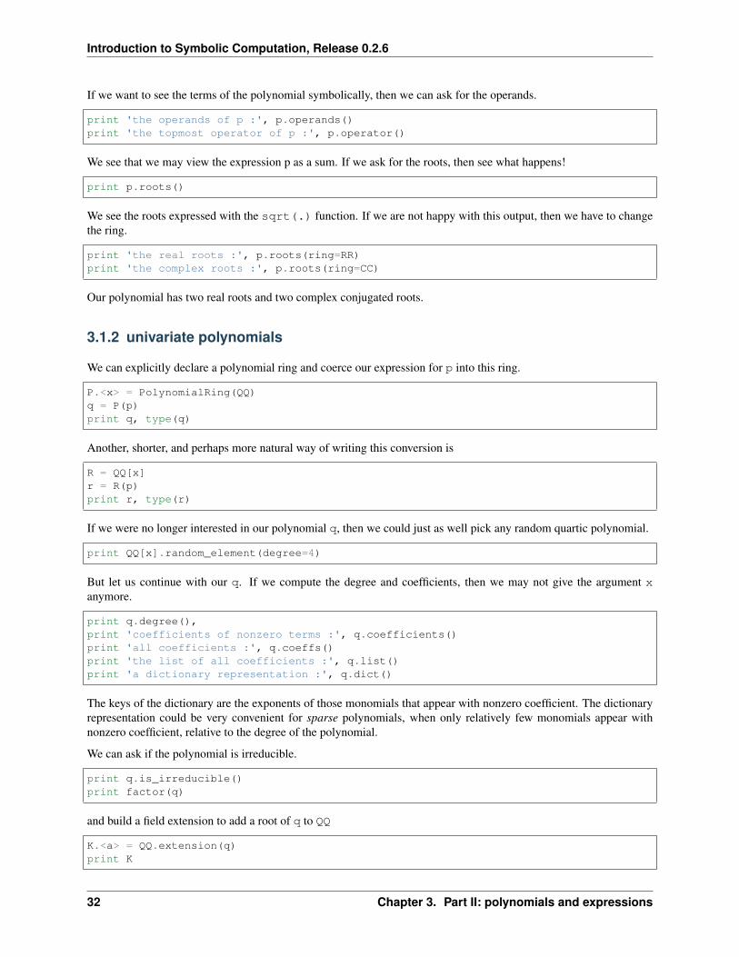
Introduction to Symbolic Computation, Release 0.2.6
If we want to see the terms of the polynomial symbolically, then we can ask for the operands.
print 'the operands of p :', p.operands()print 'the topmost operator of p :', p.operator()
We see that we may view the expression p as a sum. If we ask for the roots, then see what happens!
print p.roots()
We see the roots expressed with the sqrt(.) function. If we are not happy with this output, then we have to changethe ring.
print 'the real roots :', p.roots(ring=RR)print 'the complex roots :', p.roots(ring=CC)
Our polynomial has two real roots and two complex conjugated roots.
3.1.2 univariate polynomials
We can explicitly declare a polynomial ring and coerce our expression for p into this ring.
P.<x> = PolynomialRing(QQ)q = P(p)print q, type(q)
Another, shorter, and perhaps more natural way of writing this conversion is
R = QQ[x]r = R(p)print r, type(r)
If we were no longer interested in our polynomial q, then we could just as well pick any random quartic polynomial.
print QQ[x].random_element(degree=4)
But let us continue with our q. If we compute the degree and coefficients, then we may not give the argument xanymore.
print q.degree(),print 'coefficients of nonzero terms :', q.coefficients()print 'all coefficients :', q.coeffs()print 'the list of all coefficients :', q.list()print 'a dictionary representation :', q.dict()
The keys of the dictionary are the exponents of those monomials that appear with nonzero coefficient. The dictionaryrepresentation could be very convenient for sparse polynomials, when only relatively few monomials appear withnonzero coefficient, relative to the degree of the polynomial.
We can ask if the polynomial is irreducible.
print q.is_irreducible()print factor(q)
and build a field extension to add a root of q to QQ
K.<a> = QQ.extension(q)print K
32 Chapter 3. Part II: polynomials and expressions

Introduction to Symbolic Computation, Release 0.2.6
Now we can view the original expression as a polynomial over the new field, extended with a root of q.
q2 = K[x](q)print q2, type(q2)
See if q2 factors or not.
print q2.is_irreducible()print factor(q2)
We see that adding one algebraic number is not enough to factor completely in linear factors. Observe that we mustexplicitly coerce the nonlinear factor into a polynomial with coefficients in K.
f2 = q2/(x-a); print f2, type(f2), type(K[x](f2))L.<b> = K.extension(K[x](f2))print L
We take the original polynomial in the new extended coefficient ring and factor.
q3 = L[x](q)print factor(q3)
To select the factor to continue with our field extensions, we convert the factorization to a list.
lf = list(factor(q3))print lf
Note that the elements in the list are tuples, so we must remove the multiplicities.
f3t = lf[2]; print f3t, type(f3t)f3 = L[x](f3t[0]); print f3, type(f3)
Now make our last field extension!
M.<c> = L.extension(f3)print M
As the polynomial now factors completely, we have solved the polynomial symbolically, expressing the roots asalgebraic numbers a, b, and c.
q4 = M[x](q)print factor(q4)
The polynomial q is now factored completely as a product of linear factors, as we see (x - c) * (x - b) *(x - a) * (x + c + b + a). Observe the connection between factoring and root finding.
print q4.roots()
and we see [(c, 1), (b, 1), (a, 1), (-c - b - a, 1)]. We can still find the roots numerically ofour quartic.
crts = q4.roots(ring=CC)print crts
Because the coefficient in the term with 𝑥3 is zero, the sum of the roots in both the symbolic and the numeric repre-sentation must be zero. We can see this easily from the symbolic representation, but let us verify this on the numericalrepresentation.
3.1. Lecture 10: univariate and multivariate polynomials 33

Introduction to Symbolic Computation, Release 0.2.6
print sum(n for (n,1) in crts)
To recapitulate, we distinguish between two main forms of root finding, one is symbolic, the other numeric. Thedefault numeric field is the field of complex numbers, whereas symbolically we extend the field of rational numberswith sufficiently many symbols to represent all roots.
3.1.3 multivariate polynomials
Polynomials in several variables are declared similarly as polynomials in one variable. The quotes around the namesare needed if we have not used or declared them explicitly before as variables. We take a random polynomial of degree4, and with terms we can give an upper bound on the number of terms in the polynomial.
R.<x,y> = PolynomialRing(QQ)p = R.random_element(degree=4,terms=10)print p, type(p)
We can select the monomials, get its variables, and its degrees.
print 'the monomials :', p.monomials()print 'corresponding coefficients :', p.coefficients()print 'the variables :', p.variables()print 'the degree in x :', p.degree(x)print 'the degree in y :', p.degree(y)print 'the degree of p :', p.degree()
The order of the monomials is important.
print R.term_order()
The default order appears to be Degree reverse lexicographic term order. To change the ordering ofthe monomials in the polynomial, we coerce p into a another ring. In a lexicographic order, all monomials in which xoccurs come first.
Rlex.<x,y> = PolynomialRing(QQ,order = 'lex')print Rlex; print Rlex.term_order()print Rlex(p)
We can view a polynomial in several variables as a polynomial in one variable by collecting terms. Because of thetype of argument of polynomial(), the selection of the tuple of the outcome of p.variables() is needed.
print 'as polynomial in x :', p.polynomial(p.variables()[0])print 'as polynomial in y :', p.polynomial(p.variables()[1])
3.1.4 Assignments
1. Execute the following sequence of commands: var('x'); p = prod([x-k for k inrange(20)]); print p; q = p.expand() and then type print q.roots() and printq.roots(ring=CDF). Compare the differences between the output of the two roots. Did you expect tosee those differences?
2. Declare x as a polynomial variable over the rational number with the statement x = polygen(QQ).
(a) Give the Sage command(s) to compute the greatest common divisor of the polynomials 𝑝 = 2𝑥5+11𝑥4+14𝑥3 + 11𝑥2 + 12𝑥 and 𝑞 = 2𝑥5 + 5𝑥4 + 7𝑥3 + 8𝑥2 + 5𝑥+ 3.
34 Chapter 3. Part II: polynomials and expressions

Introduction to Symbolic Computation, Release 0.2.6
(b) How can Sage compute the cofactors 𝑘 and ℓ so that gcd(𝑝, 𝑞) = 𝑘𝑝+ ℓ𝑞?
(c) Finally, give the Sage commands to verify the relation gcd(𝑝, 𝑞) = 𝑘𝑝 + ℓ𝑞 for the 𝑘 and the ℓ that werefound.
Hint: do help(xgcd).
3. Do x = polygen(RR); print factor(x^2 - 2.25) and x = polygen(QQ); printfactor(x^2 - 9/4). Explain the differences in the outcomes of the two factor commands.
4. Consider the polynomial 𝑝 = 2𝑥5 + 9𝑥4 + 16𝑥3 + 15𝑥2 + 12𝑥+ 9. Write 𝑝 as a product of linear factors:
(a) symbolically, by adding sufficiently many formal roots; and
(b) numerically, by finding all complex roots of 𝑝.
5. Consider the polynomial 𝑝 = 2𝑥𝑧4 + 𝑥𝑧3 + 2𝑦𝑧2. Give the Sage commands to bring 𝑝 in the forms
(a) 2𝑧4𝑥+ 𝑧3𝑥+ 2𝑧2𝑦,
(b) 2𝑥𝑧4 + 𝑥𝑧3 + 2𝑧2𝑦, and
(c) 2𝑦𝑧2 + 2𝑥𝑧4 + 𝑥𝑧3.
6. Consider the polynomial 𝑝 = 𝑥3 + 4𝑥+ 7 over a finite field of 17 elements.
(a) Give the Sage commands to show that 𝑝 is irreducible over this finite field.
(b) Add sufficiently many formal roots to this finite field so that 𝑝 factors as a product of linear polynomials.
(c) Give all relevant Sage commands. Write the final factorization of 𝑝.
3.2 Lecture 11: rational functions and conversions
One of the main problems in computer algebra is expression swell.
A rational number is simplified immediately, but in rational expressions removing the greatest common denominatormay not always result in a smaller expression and may even lead to expression swell. If we consider 𝑥𝑑−1
𝑥−1 , for anydegree 𝑑 then the reason becomes clear.
3.2.1 rational expressions
Sage recognizes rational expressions as of type fraction_field_elements of sage.rings.
x = polygen(QQ)p = x^3 - 1; q = x^2 - 1; r = p/qprint r, type(r)
What is remarkable is that the rational expression is normalized automatically. The normalization of a rational expres-sion is the removal of the greatest common divisor of numerator and denominator. We see that the common factor x- 1 is removed in r.
print factor(p); print factor(q)
This automatic normalization may lead to expression swell.
f = (x^1000 - 1)/(x-1); print f
3.2. Lecture 11: rational functions and conversions 35

Introduction to Symbolic Computation, Release 0.2.6
We see an expression with 1,000 terms! Instead of printing the entire expression, we may just as well only ask for justthe number of terms. The problem is that f is still not a polynomial and we have to take its fraction before getting thenumber of coefficients.
print type(f)fn = f.numerator()print type(fn)print len(fn.coefficients())
We can freeze an expression, by conversion to a Symbolic Ring (SR).
g = SR(p)/q; print g;
This shows the original expression (x^3 - 1)/(x^2 - 1). We can ask for the denominator, with or withoutnormalization
print g.denominator(normalize=False)print g.denominator(normalize=True)
The same for the numerator, with or without normalization
print g.numerator(normalize=False)print g.numerator(normalize=True)
We may represent a rational expression with numerator and denominator in factored form, or not.
fn = g.numerator(normalize=False).factor()fd = g.denominator(normalize=False).factor()print SR(fn)/g.denominator(normalize=False)print g.numerator(normalize=False)/SR(fd)
This prints (x^2 + x + 1)*(x - 1)/(x^2 - 1) and (x^3 - 1)/((x + 1)*(x - 1)).
If we really do not want to remove common factors, then we must explicitly convert to strings.
print str(fn) + '/' + '(' + str(fd) + ')'
which shows (x^2 + x + 1)*(x - 1)/((x + 1)*(x - 1)).
3.2.2 conversions
The coercion to a symbolic ring SR on a polynomial shows the so-called Horner form of the polynomial.
x = SR.var('x')p = x^4 + 2*x^3 + 3*x^2 + 4*x + 5print p.horner(x)
The Horner form gives an efficient way to evaluate a polynomial, which requires as many multiplications as additions,for the example polynomial p, the Horner form is (((x+2)*x + 3)*x + 4)*x + 5.
The disadvantage of working with x = polygen(QQ) is that we cannot select a random element from the ring.
P.<x> = PolynomialRing(CC)rn = P.random_element(degree = 4)rd = P.random_element(degree = 4)f = rn/rdprint f, type(f)
36 Chapter 3. Part II: polynomials and expressions

Introduction to Symbolic Computation, Release 0.2.6
To evaluate a rational expression efficiently, we may consider a partial fraction decomposition.
print f.partial_fraction_decomposition()
3.2.3 assignments
1. Assign to r the expression (4*x^2 + x)/(x^2 + 4). Use the methods operands() and operator()to draw the expression tree of r.
2. Consider the rational expression p = (x^4 + x^3 - 4*x^2-4*x)/(x^4 + x^3 - x^2 - x).What are the commands to transform p into (x + 2)*(x + 1)*(x - 2)/(x^3 + x^2 - x - 1)?
3. What is the partial fraction decomposition of p = (x^4 + x^3 - 4*x^2-4*x)/(x^4 + x^3 - x^2- x)?
3.3 Lecture 12: representation of expressions
We have already covered expression trees derived from fast callable objects, but a fast callable object is just onerepresentation that is geared for evaluation in hardware arithmetic. In this lecture we examine how expressions inSage are stored internally.
3.3.1 expression trees
Let us consider again the structure of expressions.
p = x^10 + 2*x + 9print p, type(p)
We can look at the operands for the operator at the top level.
L0 = p.operands()print 'top level operands :', L0print 'with operator :', p.operator()
Then we see top level operands : [x^10, 2*x, 9] and with operator : <built-infunction add>. At the second level, we have three nodes.
L1 = [x.operands() for x in L0]print 'operands at level 1', L1print 'with operators :\n', [x.operator() for x in L0]
What is printed is operands at level 1 [[x, 10], [x, 2], []] and with operators :[<built-in function pow>, <built-in function mul>, None].
Now we can draw the expression tree for p.
add+-- pow| +-- x| +-- 10+-- mul| +-- 2| +-- x+-- 9
3.3. Lecture 12: representation of expressions 37

Introduction to Symbolic Computation, Release 0.2.6
In contrast to the expression tree of a fast_callable object, the expression tree of a general expression is not binary!
Observe the difference between the string representation and the nicely typeset form of an expression.
print pp.show()
If we coerce the expression p into a polynomial with rational coefficients and convert then into a symbolic ring (SR),then we get the Horner form.
x = SR.var('x')q = SR(p).horner(x)print q
What is printed is (x^9 + 2)*x + 9. The expression tree for q takes a different form.
L0 = q.operands()print 'operands of q :', L0print 'with operator :', q.operator()
The output is operands of q : [(x^9 + 2)*x, 9] and with operator : <built-infunction add>. Then we continue to the next level.
L1 = L0[0].operands()print 'operands of first operand :', L1print 'with operator :', L0[0].operator()
and we see operands of first operand : [x^9 + 2, x] and with operator : <built-infunction mul>. We continue one level down.
L2 = L1[0].operands()print 'operands of first operand of first operand :', L2print 'with operator :', L1[0].operator()
What is printed is operands of first operand of first operand : [x^9, 2] and withoperator : <built-in function add>. And we still have one level to go.
L3 = L2[0].operands()print 'operands of first operand of first operand of first operand :', L3print 'with operator :', L2[0].operator()
The output is operands of first operand of first operand of first operand : [x, 9]and with operator : <built-in function pow>. Then the expression tree is as follows.
add+-- mul| +-- add| | +-- pow| | | +-- x| | | +-- 9| | +-- 2| +-- x+-- 9
The Horner form does lead to a binary tree.
38 Chapter 3. Part II: polynomials and expressions

Introduction to Symbolic Computation, Release 0.2.6
3.3.2 evaluation of expressions
The form of the expression matters when it comes to evaluation. To evaluate a function at a floating point numbers,say pi.
from math import piprint p(x=pi)print q(x=pi)
Both forms of the expression give the same value 93663.33066139017. To time the evaluation, we use timeit.
timeit('p(x=pi)')
We obtain as output 625 loops, best of 3: 118 µs per loop.
timeit('q(x=pi)')
yields 625 loops, best of 3: 85.4 µs per loop. Even already on a such a small example, the Hornerform is more efficient.
Let us make a fast_callable object.
f = fast_callable(q, vars=['x'])print f(pi)
We see the same value as before. Let us time it!
timeit('f(pi)')
and this gives 625 loops, best of 3: 9.29 µs per loop.
print 'speedup of fast callable over expression :', 118/9.29
The Horner form as a fast callable object leads to a more than twelve fold speedup on a 2.5 GHz Intel Core i5 Mac OSX laptop.
3.3.3 Assignments
1. Consider p = 3*x^4 - 6*x^3 + 5*x^2 + 9*x - 7. Draw the expression tree for p. Also give allSage commands with their output used to make your drawing.
2. Consider p = 3*x^4 - 6*x^3 + 5*x^2 + 9*x - 7. Compute the Horner form q for p and draw theexpression tree for q. Also give all Sage commands with their output used to make your drawing.
3. Consider p = 3*x^4 - 6*x^3 + 5*x^2 + 9*x - 7 and its evaluation at math.pi. Compare withtimeit the efficiency of the original expression, the Horner q form of p, and the fast callable objects of p andq.
3.4 Lecture 13: substitution, expansion, and factorization
Substitution is one of the fundamental tools to work with expressions. Expansion is the counterpart of factorization.
3.4. Lecture 13: substitution, expansion, and factorization 39

Introduction to Symbolic Computation, Release 0.2.6
3.4.1 substitution
As a first application of substitution, we can replace an expression by a new variable to prevent expansion when wemanipulate expression. Substitution is normally executed in sequence, but expressions are callable objects and callingan expression by keyword arguments performs the substitution simultaneously, as required when we want to permutethe variables in an expression. Knowing the list of operands in an expression is useful. With string manipulations wecan perform a pure syntactical substitution.
Suppose we would like to rewrite (𝑥+ 𝑦)2 + 1(𝑥+𝑦)2 into (𝑥+𝑦)4+1
(𝑥+𝑦)2 .
We consider then an expression in x and y that we want to bring on the same denominator.
var('x,y')p = (x+y)^2 + 1/(x+y)^2print p, type(p)
If we want to bring the expression on a common denominator, then we could try the factor() method.
p.factor()
The output is (x^4 + 4*x^3*y + 6*x^2*y^2 + 4*x*y^3 + y^4 + 1)/(x + y)^2. The factor ex-pands the numerator, which is not what we want. To shield (x+y)^2 from expanding, we will save x+y into a newvariable z. Then we will factor the expression in z. After this, we substitute z back to x + y.
var('z')q = p.subs({(x+y): z})print 'after substitution of x+y into z :', qfq = q.factor()print 'after factoring :', fqqq = fq.subs(z=x+y)print 'after substitution of z into x+y :', qq
And we see printed as output:
after substitution of x+y into z : z^2 + 1/z^2after factoring : (z^4 + 1)/z^2after substitution of z into x+y : ((x + y)^4 + 1)/(x + y)^2
To view the expression nicely typeset, we do
qq.show()
and then we see (𝑥+𝑦)4+1(𝑥+𝑦)2 .
Observe that even when we submit a dictionary as argument of the subs() method, the substitution happens insequence and not simultaneously. Suppose we want to permute the variables in an expression. For example, we wantto replace a by b, b by c, and c by a. Then the expression a + 2*b + 3*c turns into b + 2*c + 3*a via asimultaneous substitution, that is: if the substitution is executed simultaneously. Expressions are callable objects andwhen we evaluate by keyword argument, then the substitution is executed simultaneously.
var('a,b,c')e = a + 2*b + 3*cprint 'the expression :', eprint 'substitution with dictionary argument :', e.subs({a:b, b:c, a:c})print 'evaluation by keyword arguments :', e(a=b,b=c,c=a)
The result of e.subs({a:b, b:c, a:c}) turned out to be the same as e.subs(c=a).subs(b=c).subs(a=c), but the order of the keys in dictionaries is often arbitrary.
40 Chapter 3. Part II: polynomials and expressions

Introduction to Symbolic Computation, Release 0.2.6
Returning to the first application of substitution on p, if we had tried to replace (x+y)^2 by z, then we would havenoticed that only the numerator changed. Looking at the operands of p explains why this is.
print pprint p.operands()
and we see that the list of operands is [(x + y)^2, (x + y)^(-2)].
With string manipulation, we can perform a pure syntactical substitution.
s = str(p)print st = s.replace('(x + y)^2', 'z')print t
which then shows the string z + 1/z.
Knowing the list of operands, we can substitute (x+y)^2 by z^2 and (x+y)^(-2) by z^(-1).
p.subs({(x+y)^2:z, (x+y)^(-2):z^(-1)})
which will show the expression z + 1/z.
3.4.2 expansion
When we give an expression in factored form, such as (𝑎+ 𝑏+ 𝑐)(𝑥3+9𝑥+8) then we see that Sage does not expandthe expression automatically. Why not? The main reason is expression swell.
var('a,b,c,x')p = (a + b + c)*(x^3 + 9*x + 8)print p
If we want to expand the expression, then we apply the expand() method.
print p.expand()
The expand() did too much, it expanded everything and we have lost the structure of the polynomial in x. Supposewe want to keep the factor (a + b + c) intact, what do we do then? Well, we declare a new variable and substitutethe expression a + b + c to this new variable before calling the expand() method.
var('d')dp = p.subs({a+b+c:d})print dp
Now we expand and then replace d with the original a + b + c.
edp = dp.expand()print edppp = edp.subs({d:(a+b+c)})print pp
and we see d*x^3 + 9*d*x + 8*d and (a + b + c)*x^3 + 9*(a + b + c)*x + 8*a + 8*b +8*c.
3.4. Lecture 13: substitution, expansion, and factorization 41

Introduction to Symbolic Computation, Release 0.2.6
3.4.3 factorization
The opposite to expand is factor. We distinguish between exact, symbolic, and numeric factorization. A completeexact factorization is only possible if all the roots are rational numbers.
f = factor(x^2 - 1)print f, type(f)
and we see the expression (x + 1)*(x - 1). In a symbolic factorization, we add a formal root, a so-calledalgebraic number. For example, if we start with the rational numbers, then we extend QQ with a root of an irreduciblepolynomial, using the symbol a in the extended number field K.
y = polygen(QQ)q = y^2 + 2print factor(q)print q.is_irreducible()K.<a> = QQ.extension(q)kq = (K[y])(q)print factor(kq)
Then the symbolic factorization is (x - a) * (x + a). The numerical factorization happens always over acomplex field.
z = polygen(CC)print factor(z^2 + 2)
and the numerical (approximate) factorization is (x - 1.41421356237310*I) * (x + 1.41421356237310*I).
3.4.4 assignments
1. Give the Sage commands to transform (𝑥+ 𝑦)2 + 1𝑥+𝑦 into (𝑥+𝑦)3+1
𝑥+𝑦 and vice versa.
2. Give the Sage commands to transform 𝑥2 + 2𝑥+ 1 + 1𝑥2+2𝑥+1 into (𝑥+1)4+1
(𝑥+1)2 and vice versa.
3. Give the Sage commands to transform 𝑥3 − 𝑥𝑦2 − 𝑦𝑥2 + 𝑦3 + 𝑥2 − 𝑦2 into (𝑥2 − 𝑦2)(𝑥− 𝑦 + 1).
4. Give the Sage commands to transform (𝑥+ 𝑧2 + 1)(𝑦 − 𝑧2 − 1) into 𝑥𝑦 − 𝑥(𝑧2 + 1) + (𝑧2 + 1)𝑦 − (𝑧2 + 1)2.
3.5 Lecture 14: normalizing expressions
Deciding whether two expressions represent the same mathematical object is an important problem in symbolic com-putation. We distinguish between the canonical and a normal form. Rewriting expressions using collection and sortingis a way of normalization. The quick, numerical, and probabilistic way to check whether two expressions are mathe-matically equivalent is by evaluation at a random point.
3.5.1 normal and canonical form
Expressions can take many forms. We call two expressions to be equal if they are mathematically the same.
var('x,y')e1 = x*(1+y)e2 = x + x*y
42 Chapter 3. Part II: polynomials and expressions

Introduction to Symbolic Computation, Release 0.2.6
print 'e1 = ', e1print 'e2 = ', e2print 'e1 == e1 : ', e1 == e2
From the last print we see that the equality operator == does not evaluate to True or False. We could compareidentities, but this would only result in True if both names would refer to the same object,
print id(e1) == id(e2)
which is not the case as we see False printed. If we are comparing expressions, then we could compare operandsand operators.
print e1.operands(), e1.operator()print e2.operands(), e2.operator()
But then we see [x, y + 1] <built-in function mul> for e1 and [x*y, x] <built-infunction add> for e2. At the data level, the two expressions are different.
What is we would take the difference of the two expressions?
print 'e1 - e2 :', e1 - e2
which then shows e1 - e2 : x*(y + 1) - x*y - x so Sage does not simplify. To check for equality, wecan normalize, fully expand the expressions.
ee1 = e1.expand()print 'e1 expanded :', ee1print 'e2 :', e2print 'e1 expanded - e2 :', ee1 - e2
Then the difference between the expanded e1 and the e2 leads to 0.
Expanding polynomials in several variables, for a given order of the variables and an order of the monomials, givesa normal form. Normalization is the process of bringing a mathematical expression in a normal form. For rationalexpressions we have seen that we can normalize numerator and denominator by removing common factors. A normalform is usually not unique, as we can then still represent numerator and denominator in expanded or factored form,which could lead to four different forms for the same expression.
The canonical form is the unique form of an expression. For polynomials in one variable, we can fully expand thepolynomial, remove superfluous terms (like x - x) and then sort the monomials by degree in descending order (highestdegree first).
3.5.2 rewriting multivariate polynomials
For a multivariate polynomial, once we fix the order of the variables, we can rewrite the polynomial as a polynomial inone variable, where the coefficients are polynomials in the other variables. We illustrate this on a random polynomial.
P = QQ['x,y,z']q = P.random_element(degree=5,terms=20)print q, type(q)
We see that multivariate polynomials in Sage are implemented via libSINGULAR. SINGULAR is a computer algebrapackage for computational algebraic geometry.
We can write a polynomial in several variables recursively as a polynomial in one variable with its coefficients againpolynomials in the same form.
3.5. Lecture 14: normalizing expressions 43
Introduction to Symbolic Computation, Release 0.2.6
To write the polynomial q as a polynomial in z, with coefficients polynomials in y that have coefficients in x, we do
QQ['x']['y']['z'](q)
This is another normal form for multivariate polynomials.
3.5.3 a numerical test on equality
There is a numerical probability-one test on the equality of expressions. First we generate a random point, choosingrandom complex numbers for x and y.
rx = CC.random_element()ry = CC.random_element()print 'a random point :', (rx, ry)
And then we evaluate the expressions.
v1 = e1(x=rx, y=ry)v2 = e2(x=rx, y=ry)print v1 - v2
we see 0.000000000000000 With probability one (we could have picked a point on some common factor of e1- e2), a number (close to) zero will guarantee equality of expressions. We can increase our confidence in this test bygenerating more random points and increasing the working precision of the computations.
3.5.4 assignments
1. Consider the polynomial 𝑝 = (𝑥2 + 𝑥𝑦 + 𝑥+ 𝑦)(𝑥+ 𝑦).
(a) Order the monomials in 𝑝 in total degree order, using 𝑥 > 𝑦.
(b) Order the monomials in 𝑝 in pure lexicographic order, using 𝑥 > 𝑦.
2. Consider the polynomial 𝑝 = (𝑥2 + 𝑥𝑦 + 𝑥+ 𝑦)(𝑥+ 𝑦). Rewrite 𝑝 as a polynomial in 𝑥 with coefficients in 𝑦.
3. Consider the expressions 𝑥+ 1 and (𝑥2 − 1)/(𝑥− 1).
(a) Are these expressions symbolically the same? Give the Sage commands to illustrate your answer.
(b) Verify the equality numerically. Show how a numerical equality test can go wrong.
3.6 Lecture 15: review of the first 14 lectures
In the first 14 lectures we explored the extensive number system of Sage, manipulated polynomials and general ex-pressions.
Below is a first, preliminary list of questions to review. Consider also the quizzes and homework assignments.
1. Explain the difference between 1.0 + 10**(-32) and 1 + 10**(-32).
2. The Gelfond-Schneider constant is 2√2. Give all Sage commands
(a) to compute a rational approximation for 2√2 accurate with 5 decimal places;
(b) to show that the accuracy of this approximation is indeed 5 decimal places;
44 Chapter 3. Part II: polynomials and expressions

Introduction to Symbolic Computation, Release 0.2.6
(c) to compute a sequence of 10 consecutive rational approximations, starting with 5 decimal places andincreasing in accuracy with one decimal place in each step of the sequence.
3. Explain the difference between x = polygen(QQ) and var('x').
4. Consider the polynomial 𝑝 = 97𝑥45 − 62𝑥46 − 73𝑥31. What is the best way to evaluate 𝑝 at hardware floatingpoint numbers? Give the relevant Sage commands and compare between the straightforward evaluation of theexpression for 𝑝.
5. Consider the polynomial 𝑝 = 25𝑥3 + 12𝑥2 + 26𝑥 + 4 over a finite field of size 29, similar to working modulo29.
(a) Does the polynomial factor over this field?
(b) Give the Sage commands to add sufficiently many formal roots to the field so 𝑝 has three roots over theextended number field.
(c) Write the symbolic factorization of 𝑝 in linear factors below.
6. Explain how rational expressions are normalized. Illustrate with an example.
7. Type var('x,y'); q = (x^2 - y)/(y^2 - x) and draw the expression three of q.
8. Give the Sage commands to transform (𝑥+(𝑧2+1))(𝑦−(𝑧2+1)) into 𝑥𝑦+(−𝑧2−1)𝑥+(𝑧2+1)𝑦−𝑧4−2𝑧2−1.
3.7 Lecture 16: first midterm exam
The first midterm exam covers the first two parts of the course.
3.7. Lecture 16: first midterm exam 45

Introduction to Symbolic Computation, Release 0.2.6
46 Chapter 3. Part II: polynomials and expressions

CHAPTER 4
Part III: Calculus
The third part of the course consists of a sequence of seven lectures. We call it calculus as we work with functions,used for differentiation, integration, and approximation. Giving a dictionary with as default value an empty dictionaryas last argument of a recursive functions works great for memoization.
4.1 Lecture 17: defining mathematical functions
Expressions in Sage are callable objects and for fast evaluation in machine numbers we have fast_callable objects.Although we may define functions with the Python def syntax, we can differentiate, integrate, and plot Sage functions.The simplest discontinuous functions are step functions.
4.1.1 functions in Sage and in Python
We can define functions as in Python, but also more directly.
f(x,y) = sin(x) + e^cos(y)print f, type(f)
The print f shows (x, y) |--> e^cos(y) + sin(x) and we see that a function is an expression.
print f(2,pi)sage: print f.integrate(x)
This shows e^(-1) + sin(2) and (x, y) |--> x*e^cos(y) - cos(x). Observe thus that, as we inte-grate a function, the result is again displayed as a function.
Let us explore the difference with Python functions.
def g(x,y):return sin(x) + e^cos(y)
print g, type(g)
47

Introduction to Symbolic Computation, Release 0.2.6
Now the type of g is that of function. We cannot integrate a Python function, the command below does not work.
g.integrate(x)
because the function object has no attribute integrate. But because we are defining functions in Sage, we canevaluate the function symbolically.
e = g(x,y)print e, type(e)
and we see e^cos(y) + sin(x) <type 'sage.symbolic.expression.Expression'>
So we can turn an expression into a function.
h(x,y) = eprint h, type(h)print h.integrate(x)
We see that h is defined as a function that we can integrate.
4.1.2 step functions
Can we define step functions? Step functions are the simplest discontinuous functions.
print unit_step, type(unit_step)print 'at -3 :', unit_step(-3)print 'at 4 :', unit_step(4)
The unit_step is defined in the class sage.functions.generalized.FunctionUnitStep. For nega-tive x values, the value of the unit step is zero, for positive x, the value is one. We can view the documentation stringof the class with the command:
print sage.functions.generalized.FunctionUnitStep.__doc__
The plot is perhaps the best representation of the function.
p = plot(unit_step, -1, 1)p.save('/tmp/unit_step.png')p
48 Chapter 4. Part III: Calculus

Introduction to Symbolic Computation, Release 0.2.6
The derivative of the unit step function is the Dirac delta function.
diff(unit_step(x),x)
which shows dirac_delta(x).
We can print the documentation string for the Dirac delta function:
print sage.functions.generalized.FunctionDiracDelta.__doc__
We can take the definite integral of the unit step function.
integral(unit_step(x), (x, -3, 3))
and, as expected, the integral returns 3.
Another important discontinuous function is the Kronecker delta, which is a function in two variables returning 1 ifboth arguments are equal and returning 0 otherwise.
print kronecker_delta(1,2)print kronecker_delta(1,1)
and we see 0 and 1 printed.
4.1. Lecture 17: defining mathematical functions 49

Introduction to Symbolic Computation, Release 0.2.6
4.1.3 combining functions
We can combine functions. Suppose we want to make a 3-step staircase function, defined as follows: f(x) = 0 for x <0, f(x) = 1/3 for x in [0,1), f(x) = 2/3 for x in [1,2) and f(x) = 1 for x >= 2.
f(x) = unit_step(x)/3 + unit_step(x-1)/3 + unit_step(x-2)/3plot(f(x),(x,-1,3))
4.1.4 assignments
1. Type the code below into a Sage cell. Explain what happens. Hint: consider the evaluation of a Python functionat a variable in turning an expression into a Sage function.
def h(x):if x<2:
return 0else:
return x-2plot (h(x), (x, -2, 2))
2. Make a piecewise linear function that is zero for negative values of x and takes the value x/2 for positive valuesof x.
3. Give the Sage commands to make a hat function f(x) with definition f(x) = 0 for x less than -1 or largerthan 1; and f(x) = 1 for x in the interval [-1,+1]. Make a plot to check that your definition is correct.
4.2 Lecture 18: recursive functions
Recursion is a very powerful tool to define function in a compact way. Unfortunately, a direct implementation of arecursive function may lead to very inefficient code. Using dictionaries in Python we can apply memoization andobtain efficient recursive functions without having to rewrite the recursion into an iteration.
4.2.1 memoization in Python
The Fibonacci numbers are defined recursively. The first two numbers are zero and one. The next numbers are thesum of the two previous ones. A first version as a Python function is defined below.
def fibonacci(n):"""Returns the n-th Fibonacci number."""if(n == 0):
result = 0elif(n == 1):
result = 1else:
result = fibonacci(n-1) + fibonacci(n-2)return result
Look at the first 10 Fibonacci numbers.
[fibonacci(n) for n in range(11)]
50 Chapter 4. Part III: Calculus

Introduction to Symbolic Computation, Release 0.2.6
and this shows the list of the first 10 Fibonacci numbers: [0, 1, 1, 2, 3, 5, 8, 13, 21, 34, 55].
The problem is that it gets very efficient as n grows.
timeit('fibonacci(20)')
We see 125 loops, best of 3: 6.46 ms per loop as executed on a 2.5 GHz Intel Core i5 Mac OS X10.9.4.
If we examine the tree of function calls, then we see why this definition leads to a very inefficient function. Weabbreviate fibonacci() by f().
f(5)+-- f(4)| +-- f(3)| | +-- f(2)| | | +-- f(1) = 1| | | +-- f(0) = 0| | +-- f(1) = 1| +-- f(2)| +-- f(1) = 1| +-- f(0) = 0+-- f(3)
+-- f(2)| +-- f(1) = 1| +-- f(0) = 0+-- f(1) = 1
Even for a very simple case as the 5-th Fibonacci number, we see that the f(3) gets computed thrice and f(2) twice.
With default arguments we can have functions store data. In the memoized version of the recursive Fibonacci functionwe use a dictionary to store the values for previous calls. The keys in the dictionary are the arguments of the functionand the values are what the function returns. With each call to the function, the dictionary is consulted and only ifthere is no key for the argument, then the body of the function is executed.
def memoized_fibonacci(n, D={}):"""Returns the n-th Fibonacci number, using D tomemoize the values computed in previous calls."""if D.has_key(n):
return D[n]else:
if(n == 0):result = 0
elif(n == 1):result = 1
else:result = memoized_fibonacci(n-1) + memoized_fibonacci(n-2)
D[n] = resultreturn result
Now if we time this new function.
timeit('memoized_fibonacci(20)')
we see 625 loops, best of 3: 590 ns per loop.
4.2. Lecture 18: recursive functions 51

Introduction to Symbolic Computation, Release 0.2.6
[memoized_fibonacci(n) for n in range(30)]
4.2.2 memoization in Sage
Functions in Sage can compute expressions. Chebyshev polynomials are orthogonal polynomials, available in Sagevia the function chebyshev_T.
t3 = chebyshev_T(3,x)print t3, type(t3)
and we see ‘‘ 4*x^3 - 3*x <type ‘sage.symbolic.expression.Expression’>.‘‘
The 3-terms recurrence to define Chebyshev polynomial is 𝑇 (0, 𝑥) = 1, 𝑇 (1, 𝑥) = 𝑥, 𝑇 (𝑛, 𝑥) = 2𝑥𝑇 (𝑛 − 1, 𝑥) −𝑇 (𝑛 − 2, 𝑥). The straightforward definition based on this 3-terms recurrence is below in the function T. Observe theapplication of expand().
def T(n, x):"""Returns the n-th Chebyshev polynomial in x."""if(n == 0):
return 1elif(n == 1):
return xelse:
return expand(2*x*T(n-1, x) - T(n-2, x))
To test the function, we compute the third Chebyshev polynomial.
print T(3, x)
and indeed, we see 4*x^3 - 3*x. We can check the efficiency of the implementations.
print 'the Chebyshev in Maxima :',timeit('chebyshev_T(10,x)')print 'our direct function T :',timeit('T(10,x)')
The output is
the Chebyshev in Maxima : 625 loops, best of 3: 799 µs per loopour direct function T : 25 loops, best of 3: 10.2 ms per loop
We apply the memoization technique from Python to the Sage function T and call the memoized function mT.
def mT(n, x, D = {}):"""Returns the n-th Chebyshev polynomial in x,using memoization with the dictionary D."""if D.has_key(n):
return D[n]else:
if(n == 0):result = 1
elif(n == 1):
52 Chapter 4. Part III: Calculus

Introduction to Symbolic Computation, Release 0.2.6
result = xelse:
result = expand(2*x*mT(n-1,x) - mT(n-2,x))D[n] = resultreturn result
To check its correctness, we do again print mT(3,x) to see 4*x^3 - 3*x. Let us check how much faster thememoized version is.
timeit('mT(10,x)')
and we obtain 625 loops, best of 3: 491 ns per loop.
4.2.3 assignments
1. The Bell numbers 𝐵(𝑛) are defined by 𝐵(0) = 1 and
𝐵(𝑛) =
𝑛−1∑𝑖=0
(𝑛− 1𝑖
)𝐵(𝑖),
for 𝑛 > 0. They count the number of partitions of a set of 𝑛 elements.
Write a recursive function to compute the Bell numbers. The binomial coefficient(
𝑛− 1𝑖
)is computed by
binomial(n-1,i). Make sure your procedure is efficient enough to compute B(50).
2. The Stirling numbers of the first kind 𝑐(𝑛, 𝑘) satisfy the recurrence
𝑐(𝑛, 𝑘) = −(𝑛− 1)𝑐(𝑛− 1, 𝑘) + 𝑐(𝑛− 1, 𝑘 − 1), for 𝑛 ≥ 1 and 𝑘 ≥ 1,
with the initial conditions that 𝑐(𝑛, 𝑘) = 0 if 𝑛 ≤ 0 or 𝑘 ≤ 0, except 𝑐(0, 0) = 1.
(a) Write an efficient recursive function, call it stirling1 to compute 𝑐(𝑛, 𝑘).
The 𝑛 must be the first argument of stirling1 while 𝑘 is its second argument, e.g.: for 𝑛 = 100 and𝑘 = 33, stirling1(100,33) should return 𝑐(100, 33).
(b) How many digits does the number 𝑐(100, 33) have? Give also the Sage command(s) to obtain this number.
3. The 𝑛-th Chebychev polynomial is also often defined as cos(𝑛 arccos(𝑥)).
Give the definition of the function C which takes on input the degree 𝑛 and a value for 𝑥.
Thus C(n,x) returns cos(𝑛 arccos(𝑥)) while C(10,0.512) returns the value of the 10-th Chebychev poly-nomial at 0.512. Compare this value with chebyshev_T(10,0.512).
4. Let L(n,x) denote a special kind of the Laguerre polynomial of degree n in the variable x.
We define L(n,x) by L(0,x) = 1, L(1,x) = x, and for any degree n > 1: n*L(n,x) =(2*n-1-x)*L(n-1,x) - (n-1)*L(n-2,x).
Write a Sage function Laguerre that returns L(n,x). Make sure your function can compute the 50-thLaguerre polynomial.
5. Denote the composite Trapezoidal rule for∫ 𝑏
𝑎𝑓(𝑥)𝑑𝑥 using 2𝑛 intervals by T(n,f,a,b).
We can define T(n,f,a,b) recursively by two rules: T(0,f,a,b) = (f(a) + f(b))*(b-a)/2 andT(n,f,a,b) = T(n-1,f,a,(a+b)/2) + T(n-1,f,(a+b)/2,b), for n > 0.
(a) Write a recursive Sage function for T.
4.2. Lecture 18: recursive functions 53

Introduction to Symbolic Computation, Release 0.2.6
(b) Explain how you can define T so that f is never evaluated twice at the same point.
Illustrate using n = 5 in T for the numerical approximation of∫ 1
0cos(𝑥)𝑑𝑥.
4.3 Lecture 19: working with functions
List comprehensions in Python take the form [f(x) for x in L] where L is some list and f some function. Theresult is a new list that contains all function values of f(x) for all elements x in the list L. In Sage we can apply listcomprehensions to build expressions of arbitrary size and shape.
4.3.1 list comprehensions
We can use a list comprehension to create a sequence of 20 variables, starting from x01, x02, .., x20.
v = [var('x' + '%02d' % k) for k in range(1,21)]print v
Observe the string concatenation with the proper formatting of the integer index. This leads to thelist [x01, x02, x03, x04, x05, x06, x07, x08, x09, x10, x11, x12, x13, x14, x15,x16, x17, x18, x19, x20]. Now we raise every variable to the power three.
p = [x^3 for x in v]print p
and we computed [x01^3, x02^3, x03^3, x04^3, x05^3, x06^3, x07^3, x08^3, x09^3,x10^3, x11^3, x12^3, x13^3, x14^3, x15^3, x16^3, x17^3, x18^3, x19^3, x20^3].We add up the powers into a sum to make an expression.
e = sum(p)print e, type(e)
The sum leads to the expression x01^3 + x02^3 + x03^3 + x04^3 + x05^3 + x06^3 + x07^3 +x08^3 + x09^3 + x10^3 + x11^3 + x12^3 + x13^3 + x14^3 + x15^3 + x16^3 + x17^3+ x18^3 + x19^3 + x20^3. We can return to the list representation via the operands() method.
ope = e.operands()print ope, type(ope)
and this gives a list [x01^3, x02^3, x03^3, x04^3, x05^3, x06^3, x07^3, x08^3, x09^3,x10^3, x11^3, x12^3, x13^3, x14^3, x15^3, x16^3, x17^3, x18^3, x19^3, x20^3].Raising the k-th operand to the power k goes as follows.
r = [ope[k]^k for k in range(len(ope))]print r
and then we see [1, x02^3, x03^6, x04^9, x05^12, x06^15, x07^18, x08^21, x09^24,x10^27, x11^30, x12^33, x13^36, x14^39, x15^42, x16^45, x17^48, x18^51,x19^54, x20^57]. Note that all operands are expressions.
print r[2], type(r[2])print r[2].degree(v[2])
With the proper selection of the variable in the argument of degree() we get the right degree, which is 6 for r[2].We can compute the degrees in their variables.
54 Chapter 4. Part III: Calculus

Introduction to Symbolic Computation, Release 0.2.6
print [(r[k]).degree(v[k]) for k in range(len(ope))]
which leads to [0, 3, 6, 9, 12, 15, 18, 21, 24, 27, 30, 33, 36, 39, 42, 45, 48, 51,54, 57].
Suppose we want to select those operands of degree less than 13. Recall the unit_step() function.
print r[2], ':', unit_step(13 - r[2].degree(v[2]))print r[8], ':', unit_step(13 - r[8].degree(v[8]))
and we see x03^6 : 1 and x09^24 : 0. Now we can remove all operands with degree higher than 13.
filter = lambda x, k: x*unit_step(13 - x.degree(v[k]))s = [filter(r[k],k) for k in range(len(r))]print s
and we see [1, x02^3, x03^6, x04^9, x05^12, 0, 0, 0, 0, 0, 0, 0, 0, 0, 0, 0, 0,0, 0, 0] and then build the expression again with sum().
t = sum(s)print t
and we obtain x05^12 + x04^9 + x03^6 + x02^3 + 1.
4.3.2 composing functions
Consider the trajectory of a projectile in space modeled by a parabola, subject to the following constraints. At time t =0 it is launched from the ground and at time t = 45 it hits the ground 120 miles further. Assuming constant horizontalspeed we create a function f(t) to give the altitude of the projectile in function of time. First we model the shape of thetrajectory.
y(x) = x*(120 - x)p = plot(y(x), (x, 0, 120))p.save('/tmp/trajectory.png')p
The plot saved in /tmp/trajectory.png is
4.3. Lecture 19: working with functions 55

Introduction to Symbolic Computation, Release 0.2.6
Now we want a function in time t. The assumption of constant horizontal speed implies that x is just a rescaling of t.This means that when t = 45, x must be 120.
x(t) = 120/45*tprint 'x at 0 :', x(0)print 'x at 45 :', x(45)
and indeed, we see x at 0 : 0 and x at 45 : 120 printed. Then the altitude is given as the compositionof y after x.
f(t) = y(x(t))print 'altitude at 0 :', f(0)print 'altitude at 22.5 :', f(22.5)print 'altitude at 45 :', f(45)
as altitudes at 0, 22.5, and 45, we respectively see 0, 3600.00000000000 and 0. With the composition of functionswe have separated the geometric shape of the trajectory and its evolution in time. Suppose we want to halve the speed.
h(t) = t/2hf(t) = f(h(t))print 'altitude at 45 :', hf(45)print 'altitude at 90 :', hf(90)
and the prints confirm that the projectile reaches its peak at 45 and falls to the ground at 90.
We can also make a 3d-plot of the space curve.
56 Chapter 4. Part III: Calculus

Introduction to Symbolic Computation, Release 0.2.6
p3 = parametric_plot3d([x(t), 0, f(t)], (t, 0, 45))p3.save('/tmp/trajectory3d')p3
and this shows the following image:
4.3.3 functions returning functions
We can define functions that return functions. Suppose we are interested in solving equations with Newton’s method.
def newton_step(f, x):"""Returns the function that will perform one Newton step
4.3. Lecture 19: working with functions 57

Introduction to Symbolic Computation, Release 0.2.6
to solve the equation f(x) = 0."""n(x) = x - f(x)/diff(f,x)return n
Let us try it out on the square function, so we can compute the square root of two.
sqr(x) = x^2 - 2our_sqrt = newton_step(sqr, x)print our_sqrt
Then we see x |--> x - 1/2*(x^2 - 2)/x. Observe that if we start at an integer value, we get rationalapproximations for the square root of two.
our_sqrt(our_sqrt(our_sqrt(2)))
Starting at 2, three iterations of Newton’s method yields 577/408. For a repeated application of a function, wemultiply strings.
s = 'our_sqrt('*5 + '2' + ')'*5print s
We will then execute our_sqrt(our_sqrt(our_sqrt(our_sqrt(our_sqrt(2))))) and we evaluate theexpression.
v = eval(s)print v
This gives 886731088897/627013566048. To compare with an actual approximation for sqrt(2).
print v.n(digits=30)print sqrt(2).n(digits=30)
and we see
1.414213562373095048801689623501.41421356237309504880168872421
4.3.4 assignments
1. Type L = [randint(0,99) for i in range(10)] to generate a list of 10 random numbers between0 and 99. Give the Sage commands for the following operations.
(a) divide every element in the list by 100;
(b) convert the list to a list of floating-point numbers of a precision of 3 decimal places;
(c) select all elements in the list that are larger than 0.5;
(d) compute the sum of the elements in the list.
2. The command is_prime() applied to a number returns True if the number is prime and False otherwise.Use is_prime() to make a list of all primes less than 1000. How many 3-digit primes are there?
3. Do P.<x> = PolynomialRing(RR, sparse=False) and q = P.random_element(degree=10). Select from q all terms with positive coefficients and make a newpolynomial with those terms.
58 Chapter 4. Part III: Calculus

Introduction to Symbolic Computation, Release 0.2.6
4. Let 𝑛 and 𝑘 be positive natural numbers with 𝑘 < 𝑛 and consider the polynomial𝑛−1∑𝑖=0
𝑘−1∏𝑗=0
𝑧(𝑖+𝑗) mod 𝑛.
Define a function that takes on input a list of variables (where 𝑛 is the length of the list) and a value for 𝑘. Onoutput is the expression as defined by the polynomial above. Hint: use prod to make the product of a list ofexpressions.
Show the result of your function on a sequence of 10 variables and for 𝑘 = 3.
5. Execute the newton_step function on the our_sqr function, defined again as x^2 - 2. Newton’s methodhas the property of converging quadratically, that is: in each step the correct number of decimal places doubles.Starting at 2, perform 10 steps with Newton’s method and verify the progess of the accuracy of the rationalapproximations for the square root of 2? Do you observe quadratic convergence?
4.4 Lecture 20: symbolic and numeric differentiation
We can take derivatives symbolically, of expressions and functions. Numerically, we work with difference formulas.Some functions are defined implicitly, as the solution of some equation. Declaring some variables as functions ofothers, we can derive the equation and solve for the derivative. This is implicit differentiation.
4.4.1 symbolic differentiation
We can compute the derivative of an expression with diff, which is an alias for the derivative method.
print 'the derivative of cos(x) is', diff(cos(x),x)
and we see that the derivative of cos(x) is -sin(x). For repeated differentiation, we have an extraargument.
[diff(cos(x), x, k) for k in range(5)]
and this list comprehension returns [cos(x), -sin(x), -cos(x), sin(x), cos(x)]. We can computederivatives of functions.
f(x,y) = x^2*y + 2*x*y + xprint 'f =', fprint 'the derivative of f is', f.diff()
The function f = (x, y) |--> x^2*y + 2*x*y + x has as its derivative (x, y) |--> (2*x*y +2*y + 1, x^2 + 2*x). We see that the derivative of a function in two variables returns a function that returns atuple of two expressions.
print f.diff(x)print f.diff(y)
and we see the two partial derivatives (x, y) |--> 2*x*y + 2*y + 1 with respect to x and (x, y) |-->x^2 + 2*x with respect to y. What if we take the derivative twice?
print f.diff().diff()
we get
[ (x, y) |--> 2*y (x, y) |--> 2*x + 2][(x, y) |--> 2*x + 2 (x, y) |--> 0]
4.4. Lecture 20: symbolic and numeric differentiation 59

Introduction to Symbolic Computation, Release 0.2.6
The matrix of second order derivatives of a function in several variables is called the Hessian. To compute an elementin the matrix we give names of variables as arguments to the diff.
print f.diff(x).diff(y)
and we obtain 𝜕𝑓𝜕𝑥𝜕𝑦 as (x, y) |--> 2*x + 2.
4.4.2 numerical differentiation
Numerical differentiation is available in scipy.misc, in the derivative method.
from scipy.misc import derivative as numdifprint 'exact derivative :', -sin(1.0)print '1st order approx :', numdif(func=cos(x), x0=1.0, dx=1.0e-2)
and we then see
exact derivative : -0.8414709848078971st order approx : -0.841456960361603
The numerical differentiation uses central differences. With extrapolation we can improve the accuracy.
ND = [numdif(func=cos(x), x0=1.0, dx=1.0e-2, order=k) for k in range(3, 12, 2)]for a in ND: print aprint -sin(1.0)
what is printed is below
-0.841456960361603-0.841470984527404-0.841470984807883-0.841470984807891-0.841470984807884-0.841470984807897
4.4.3 implicit differentiation
We can declare derivatives symbolically. Assume one variable y is a function of another variable x.
x = var('x')y = function('y')(x)dy = y.diff(x)print dy, type(dy)
Then dy is a symbolic expression, shown as diff(y(x),x). The application is implicit differentiation.
circle = x^2 + y^2 - 1 == 0print circle, type(circle)
That y is a function of x shows in the display of the equation x^2 + y(x)^2 - 1 == 0. This equation defineshow y depends on x. Then we differentiate the equation.
dc = circle.diff(x)print dc
60 Chapter 4. Part III: Calculus

Introduction to Symbolic Computation, Release 0.2.6
The equation we now can solve for dy is
2*y(x)*diff(y(x),x) + 2*x == 0
Thus we solve for the derivative.
yx = solve(dc, dy)print yx
The solution is
[diff(y(x),x) == -x/y(x)]
4.4.4 assignments
1. Give the Sage command to compute𝜕8𝑓
𝜕5𝑥𝜕3𝑦for 𝑓(𝑥, 𝑦) = 𝑒2𝑥+cos(𝑦).
2. Consider the curve defined by the equation 3 + 2 x + y + 2 x^2 + 2 x y + 3 y^2 = 0. Locallywe can view y as a function of x, that is: y = y(x). Compute formulas for the first and the second derivativeof y with respect to x.
3. Consider the curve defined by the equation 𝑥3−𝑦2+𝑥 = 0. The point 𝑃 with coordinates
(1
2,
√10
4
)satisfies
the equation and thus lies on the curve. Compute the first and second derivatives of the curve evaluated at 𝑃 .Give the values and the Sage commands.
4. Consider the plane curve defined by 𝑝(𝑥, 𝑦) = 𝑥4𝑦2 − 𝑥2𝑦3 + 𝑥 − 𝑦 = 0. Locally at the point (1, 1), we view𝑦 as a function of 𝑥, that is: as 𝑦(𝑥).
Compute𝑑𝑦
𝑑𝑥. What is the value for 𝑦′(1) =
𝑑𝑦
𝑑𝑥
𝑥=1
?
4.5 Lecture 21: integration and summation
Integrals occur everywhere in science and engineering. In case there is no symbolic antiderivative, we can approximatethe value for a definite integral with numerical techniques.
4.5.1 indefinite and definite integrals
The counterpart to derivative is integral.
integral(cos(x),x)
and we see sin(x). We can verify that integration is anti-differentiation and differentiation is anti-integration.
print diff(integral(cos(x),x),x)print integral(diff(cos(x),x),x)
in both cases we see cos(x). Not every expression has a symbolic antiderivative.
4.5. Lecture 21: integration and summation 61

Introduction to Symbolic Computation, Release 0.2.6
e = cos(exp(x^2))i = integral(e,x)print 'the anti-derivative of', e, 'is', i
and Sage prints
the anti-derivative of cos(e^(x^2)) is integrate(cos(e^(x^2)), x)
We can look for the definite integral of the expresion.
d = integral(e, (x, 0, 1))print dd.show()
and we see∫ 1
0cos(𝑒(𝑥
2))𝑑𝑥.
Numerical integration gives an approximation for the definite integral.
print d.n()
and we see 0.112823456937.
4.5.2 assisting the integrator
We can compute definite integrals symbolically.
var('a, b')print integral(x^2, (x, a, b))
The cubic polynomial -1/3*a^3 + 1/3*b^3 equals the area under the parabola y = x^2 for all x ranging froma till b. That does not work always so well. Sometimes we have to assist the integrator.
var('a, b')print integral(1/x^2, (x, a, b))
The exception triggered is ValueError with the comment that Computation failed since Maximarequested additional constraints; and moreover: using the 'assume' commandbefore evaluation *may* help (example of legal syntax is 'assume(b-a>0)', see`assume?` for more details)
Before we continue to examine the exception thrown by Sage, let us not see if we cannot apply the fundamentaltheorem of calculus: (1) compute the antiderivative; and then (2) make the difference of the antiderivatives evaluatedat the end points.
ad = integral(1/x^2,x)print adprint ad(x=b) - ad(x=a)
The antiderivate is -1/x and evaluated at the end points, this gives us 1/a - 1/b. So why does Sage now complainabout the original definite integral? The answer is in the following plot, recall that the definite integral gives the areaunder the curve defined by 1/x^2 for all x in [a,b]. Let us take [-2, 3] for the interval.
plot(1/x^2, (x, -2, 3))
62 Chapter 4. Part III: Calculus

Introduction to Symbolic Computation, Release 0.2.6
The plot shows there is something happening in the interval [-2, 3]. Now that we understand that the fundamentaltheorem of calculus does not apply for just any interval [a,b], we can look at the exception Sage raised when weasked for the definite integral.
The question we see in the worksheet is
Is b-a positive, negative or zero?
We see that Sage asks about the sign of b-a. We can add assumptions to variables.
assume(a > 0, b > a)print integral(1/x^2, (x, a, b))
and then we have the value 1/a - 1/b. We can check the assumptions.
assumptions()
and we then see [a > 0, b > a]. Assumptions are removed with forget.
forget(b > a)print assumptions()forget(a > 0)print assumptions()
We then see printed:
[a > 0][]
4.5.3 symbolic summation
Sage can find explicit expressions for formal sums. Suppose we want to sum k for k going from 1 to n, denoted as𝑛∑
𝑘=1
𝑘.
var('k, n')s = sum(k, k, 1, n)print sf = s.factor()print f
What is printed is 1/2*n^2 + 1/2*n and 1/2*(n + 1)*n With range and the ordinary Python sum, we canverify the formulas, say for n = 100.
print sum(range(1, 101))print f(n = 100)
and in both cases we see 5050 as the sum.
We end with a more interesting formal sum. Infinity is expressed as oo.
sum(1/k^2, k, 1, oo)
and thus we see that∞∑𝑘=1
1
𝑘2=
𝜋2
6. With list comprehensions, we can verify the symbolic sum with a numerical
example.
4.5. Lecture 21: integration and summation 63

Introduction to Symbolic Computation, Release 0.2.6
L = [float(1/k^2) for k in range(1, 100001)]print sqrt(6*sum(L))
and then we see 3.14158310433.
4.5.4 assignments
1. Compute∫𝑥𝑛𝑒𝑥𝑑𝑥 for a general integer 𝑛. Check the result for some randomly chosen values for 𝑛.
2. Let 𝐹 be the function defined by 𝐹 (𝑇 ) =
∫ 𝑇
1
exp(−𝑡2𝑇 )
𝑡𝑑𝑡.
(a) Define the Sage function 𝐹 to compute 𝐹 (𝑇 ). Use it to compute a numerical approximation for 𝐹 (2).
Compare the approximation for 𝐹 (2) to the approximation for∫ 2
1
exp(−2𝑡2)
𝑡𝑑𝑡.
(b) Compute the derivative function of 𝐹 . What is a numerical approximation of 𝐹 ′(2)? Compare the value𝐹 ′(2) to 𝐹 (2+ℎ)−𝐹 (2)
ℎ for sufficiently small values of ℎ.
3. Compute∫ ∞
0
ln(𝑥)
(𝑥+ 𝑎)(𝑥− 1)𝑑𝑥 for positive 𝑎.
4. Show that𝑛∑
𝑘=1
𝑘3 =1
4𝑛2(𝑛+ 1)2.
5. Compare the results of∫ (∫
𝑥− 𝑦
(𝑥+ 𝑦)3𝑑𝑥
)𝑑𝑦 with
∫ (∫𝑥− 𝑦
(𝑥+ 𝑦)3𝑑𝑦
)𝑑𝑥. Why are the expressions differ-
ent?
Compute∫ 1
0
(∫ 1
0
𝑥− 𝑦
(𝑥+ 𝑦)3𝑑𝑥
)𝑑𝑦 with
∫ 1
0
(∫ 1
0
𝑥− 𝑦
(𝑥+ 𝑦)3𝑑𝑦
)𝑑𝑥. Is there a correct value for the integral?
4.6 Lecture 22: series, approximations, and limits
The manipulation of series is a form of hybrid exact-approximation computation.
4.6.1 Taylor series
Let us construct a taylor series for sin(x) of order 6 at x = 0.
tsin = taylor(sin(x), x, 0, 6)print tsin, type(tsin)
and we see 1/120*x^5 - 1/6*x^3 + x That the result of a taylor is an expression makes it easy for evaluation.Close to zero, this will approximate the true sine function up to 6-th order.
a = tsin(0.01)b = sin(0.01)print a, b, abs(a-b)
which shows the numbers 0.00999983333416667, 0.00999983333416666, and 1.73472347597681e-18 as the magnitude for the error. We can do this pure formally, on an arbitrary function f inx, at some point a.
64 Chapter 4. Part III: Calculus

Introduction to Symbolic Computation, Release 0.2.6
var('x, a')f = function('f')(x)tf = taylor(f(x), x, a , 4)print tf, type(tf)
so we get the general form of a Taylor expansion of any function f in x at a as
1/24*(a - x)^4*D[0, 0, 0, 0](f)(a) - 1/6*(a - x)^3*D[0, 0, 0](f)(a)+ 1/2*(a - x)^2*D[0, 0](f)(a) - (a - x)*D[0](f)(a) + f(a)
The Fibonacci numbers arise as the coefficient of the Taylor series of a particular rational function. To see the first 10Fibonacci numbers, we can do
g = x/(1-x-x^2)tg = taylor(g(x), x, 0, 10)print tgprint tg.coefficients()
The Taylor series is 55*x^10 + 34*x^9 + 21*x^8 + 13*x^7 + 8*x^6 + 5*x^5 + 3*x^4 +2*x^3 + x^2 + x `` and the coefficients (with corresponding exponents) is arein the list ``[[1, 1], [1, 2], [2, 3], [3, 4], [5, 5], [8, 6], [13, 7], [21,8], [34, 9], [55, 10]]. Taylor series are defined for expressions in several variables as well. For example,consider cos(x)*sin(y) at x = pi/2 and y = 0.
var('x,y')h = cos(x)*sin(y)print taylor(h,(x,pi/2),(y,0),5)
and we get -1/48*(pi - 2*x)^3*y - 1/12*(pi - 2*x)*y^3 + 1/2*(pi - 2*x)*y.
4.6.2 Taylor series in SymPy
Let us see what systems Sage uses to compute the Taylor series.
from sage.misc.citation import get_systemsget_systems('taylor(sin(x), x, 0, 6)')
and we see ['ginac', 'Maxima'].
Also SymPy exports Taylor series in a more Pythonic way with generators.
from sympy.series import seriesprint series(sin(x), x0=0, n=10)
and the tenth order Taylor series for sin(x) at zero is x - x**3/6 + x**5/120 - x**7/5040 + x**9/362880 + O(x**10). If instead of n=10 for the order, we give None as argument, we obtain a generator:
g = series(sin(x), x0=0, n=None)print g, type(g)
and we see that g is a generator object. We can use a generator with the next() method to get the next term in theseries.
print g.next()print g.next()
4.6. Lecture 22: series, approximations, and limits 65

Introduction to Symbolic Computation, Release 0.2.6
or in a list comprehension to get the next 5 terms in the series
[g.next() for k in range(5)]
4.6.3 power series
In Sage, Taylor series are not power series, but we can turn any polynomial into a power series.
var('x')q = x^3 + 3*x + 8pq = q.power_series(QQ)print pq, type(pq)
and then pq is shown as 8 + 3*x + x^3 + O(x^4) and of type sage.rings.power_series_poly.PowerSeries_poly. Why would we want to turn a polynomial into a power series? Well, unlike polynomials,every power series has an inverse and there is a division operator for power series.
ipq = 1/pqprint ipq, type(ipq)print pq*ipq
The inverse of the series pq leads to 1/8 - 3/64*x + 9/512*x^2 - 91/4096*x^3 + O(x^4) of thesame type as pq. The multiplication leads to 1 + O(x^4). The order of a series is also known as its precision andwe can query the precision by the prec() method.
print pq.prec(), ipq.prec()
So both series are of precision 4. Note that the order is not equal to the degree.
print pq.degree()
While the order is 4, the degree is 3.
Truncating to a series of lower precision happens with truncate_powerseries().
tipq = ipq.truncate_powerseries(2)print tipq, type(tipq)
1/8 - 3/64*x + O(x^2) <type ‘sage.rings.power_series_poly.PowerSeries_poly’> We can turn a power series into apolynomial with the polynomial() method, or we can truncate to a certain precision.
print ipq.polynomial()print ipq.truncate(2)
With polynomial() we see -91/4096*x^3 + 9/512*x^2 - 3/64*x + 1/8 and truncate(2) gives-3/64*x + 1/8.
With r = p.reverse() we compute a power series r so that when r is substituted in p, a series of order k, weobtain x + O(x^k). The series p should not have a nonzero constant term. The coefficients of a series can selectwith list. Of our example pq, we substract list(pq)[0] to remove the constant term.
print pqprint 'the coefficients of the series :', list(pq)pq1 = pq - list(pq)[0]r = pq1.reverse()print r
66 Chapter 4. Part III: Calculus

Introduction to Symbolic Computation, Release 0.2.6
What is printed as r is 1/3*x - 1/81*x^3 + O(x^4). Let us verify the reversion of the series by substitution:Note that it works both ways.
pq1(x = r)r(x = pq1)
and we see x + O(x^4) twice.
4.6.4 approximations
Padé approximations are rational approximations.
z = PowerSeriesRing(QQ, 'z').gen()pd = exp(z).pade(4,4)print pd, type(pd)
and then we see (z^4 + 20*z^3 + 180*z^2 + 840*z + 1680)/(z^4 - 20*z^3 + 180*z^2- 840*z + 1680). as an object of the class sage.rings.fraction_field_element.FractionFieldElement_1poly_field. How good are the approximations, let us evaluate at 3.14.
print pd(3.14)print exp(3.14)
and we see that we have two decimal places correct:
23.068151742694923.1038668587222
4.6.5 limits
We can take limits with the limit command. For example, consider the limit definition of the transcendental constant
𝑒 = lim𝑘→∞
(1 +
1
𝑘
)𝑘
.
var('k')f = (1+1/k)^kf.limit(k=oo)
and as output we see e.
4.6.6 assignments
1. Make a 10-th order Taylor series of arctan(𝑥) about 𝑥 = 0. Compute the difference between the value of Taylorseries evaluated at 0.3 and arctan(0.3).
2. Use the series method of SymPy to make a generator for the Taylor series of x/(1-x-x^2) that has theFibonacci numbers as coefficients. Apply the generator in a list comprehension to compute the first 50 Fibonaccinumbers.
3. Use Sage to verify that1√
1− 4𝑥=∑𝑛≥0
(2𝑛𝑛
)𝑥𝑛 in the following way:
(a) Compute a 7-th order Taylor series of of1√
1− 4𝑥about 𝑥 = 0.
4.6. Lecture 22: series, approximations, and limits 67
Introduction to Symbolic Computation, Release 0.2.6
(b) Compute∑𝑛≥0
(2𝑛𝑛
)𝑥𝑛 for 𝑛 = 7.
4. The binomial coefficient(
𝑛+ 𝑘𝑘
)counts all choices of 𝑘 elements from a set of 𝑛+ 𝑘 elements and can be
defined via a Taylor series expansion of 𝑔(𝑧) =1
(1− 𝑧)𝑛+1at 𝑧 = 0. Verify this definition for 𝑛 = 10 and all
values for 𝑘 ranging from 0 to 10.
5. Compare the accuracy of a Padé approximation for sin(𝑥) of (4,4) with the accuracy of a fourth order Taylorseries for sin(𝑥). Compare with a plot of sin(𝑥) on the interval [0, 2].
4.7 Lecture 23: symbolic-numeric computation
With interval arithmetic we compute floating-point approximations and estimates for the errors. The manipulation ofsymbolic expressions is used to formulate equations to solve, which we illustrate via the application of the Lagrangemultiplier technique to a constrained optimization problem.
4.7.1 interval arithmetic
There is one important type of arithmetic we have not covered yet, and that is interval arithmetic.
R = RealIntervalField()print R
and R is a Real Interval Field with 53 bits of precision. By default, theRealIntervalField() without argument (also abbreviated as RIF) works with double precision floating-point arithmetic. We can coerce or convert into this field.
api = R(pi)print api, type(api)print api.str(style='brackets')
and we respectively see 3.141592653589794? (observe the question mark at the end) and the interval[3.1415926535897931 .. 3.1415926535897936] as a RealIntervalFieldElement of sage.rings.real_mpfi.
Interval arithmetic provides operations to add, substract, multiply, and divide intervals. The width of the intervalgives an upper bound on the roundoff error. With interval arithmetic we compute at the same time a floating-pointapproximation and an estimate for the error on this approximation.
To motivate the use of interval arithmetic, we take an example from the paper of Stefano Taschini in the proceedingsof SciPy 2008. We convert the floating-point coefficients to rational numbers.
F(x,y) = (QQ(333.75) - x**2)*y**6 + x**2*(11*x**2*y**2 - 121*y**4 - 2)+ QQ(5.5)*y**8 + x/(2*y)print F(A, B) = (77617, 33096)exact = F(A, B)print 'the exact value :', exact, RDF(exact)
and the exact value is -54767/66192 or approximated in double precision -0.827396059947. With increasingmultiprecision, we may gain more confidence in the results.
68 Chapter 4. Part III: Calculus

Introduction to Symbolic Computation, Release 0.2.6
f53 = F(A.n(53), B.n(53))print f53for k in range(54, 105, 10):
print F(A.n(k), B.n(k))
and we see
3.62381792172646e20-8.18209863729137e203.64375473385373696e171.46852011835392000000e146.72051363840000000000000e109.62723840000000000000000000e7-196610.0000000000000000000000000
Let us continue.
for k in range(100, 130, 5): print F(A.n(k), B.n(k))
and then we get the following:
3.9976940000000000000000000000e665534.00000000000000000000000000-2.0000000000000000000000000000000-2.000000000000000000000000000000000-2.0000000000000000000000000000000000-0.7500000000000000000000000000000000000
The sequence of repeated -2.0 values is especially troublesome as one would reach the wrong conclusion that theprecision is enough once the sequence has stabilized. This trial and error process is not really encouraging...
R = RealIntervalField(130)z = F(R(A), R(B))print R(z).str(style='brackets')
and we get
[-0.82812500000000000000000000000000000000000 ..-0.82031250000000000000000000000000000000000]
4.7.2 constrained optimization
The method of Lagrange multipliers allows to solve a constrained optimization problem.
var('x,y,z')target = x^2 + 2*x*y*z - z^2constraint = x^2 + y^2 + z^2 - 1 == 0print 'optimize', target, 'subject to', constraint
and we get the printed message optimize 2*x*y*z + x^2 - z^2 subject to x^2 + y^2 + z^2 -1 == 0. To apply the method of Lagrange multipliers, we need to compute the gradients. For this, we convert theexpressions into functions. Observe that the constraint was given as an equation, so we must select the left hand sideof the equation when we convert the expression to a function.
4.7. Lecture 23: symbolic-numeric computation 69

Introduction to Symbolic Computation, Release 0.2.6
ft(x,y,z) = targetfc(x,y,z) = constraint.lhs()print 'target as function :', ftprint 'constraint as function :', fcgt = ft.diff()gc = fc.diff()print 'gradient of target :', gtprint 'gradient of constraint :', gc
and the results are
target as function : (x, y, z) |--> 2*x*y*z + x^2 - z^2constraint as function : (x, y, z) |--> x^2 + y^2 + z^2 - 1gradient of target : (x, y, z) |--> (2*y*z + 2*x, 2*x*z, 2*x*y - 2*z)gradient of constraint : (x, y, z) |--> (2*x, 2*y, 2*z)
Now we set up the system.
var('w')eqs = [gt(x,y,z)[k] - w*gc(x,y,z)[k] == 0 for k in range(3)]eqs.append(constraint)print eqs
The polynomial system we obtain is thus
[-2*w*x + 2*y*z + 2*x == 0, -2*w*y + 2*x*z == 0,2*x*y - 2*w*z - 2*z == 0, x^2 + y^2 + z^2 - 1 == 0]
and then we just do solve...
sols = solve(eqs,{x,y,z,w})print solsprint 'found', len(sols), 'solutions'
to see that Sage found 14 solutions.
4.7.3 assignments
1. Do x = RIF(-1, +1); print 1/x. Interpret the result.
2. Compare the evaluation of 𝑝 = 𝑥2 − 4𝑥 and 𝑞 = 𝑥(𝑥− 4) at the interval [1, 4]. Which form of the expression,𝑝 or 𝑞 leads to the most accurate result? Justify your answer.
3. Find those points on the surface 𝑥2 − 𝑥𝑦 + 𝑦2 − 𝑧2 = 1 closest to the origin. Set up the system with Lagrangemultipliers and solve.
4. Consider the surface defined by 𝑔(𝑥, 𝑦) = 𝑥2 + 3𝑥𝑦 + 2𝑦2 + 7𝑥 = 0. Find those points (𝑥, 𝑦) that satisfy𝑔(𝑥, 𝑦) = 0 and that are closest to the origin.
(a) Give the Sage command(s) to define this problem as a polynomial system.
(b) Give the Sage command(s) to bring this system in triangular form. How many solutions can this systemhave? Justify your answer.
(c) Find all real solutions.
70 Chapter 4. Part III: Calculus

CHAPTER 5
Part IV: plotting and solving equations
In this part we start to use Sage as a true mathematical software system. We model a mathematical problem, applyadvanced solvers, and visualize the setup and the computational results. This covers roughly week 9 and week 10 ofthe course, we have completed two thirds. This part ends with the second midterm exam.
5.1 Lecture 24: two dimensional plots
Plotting is one of the main strengths of computer algebra systems. We distinguish between plotting formulas andfunctions. Similar to function and expressions in one variable, curves in the plane are best plotted when given inparametric form. For curves with singularities at the origin, the conversion into a polar form may lead to much betterresults, because then we can factor out the singular point in the polar formulation.
5.1.1 plotting formulas and functions
Note there is a difference in syntax between plotting expressions and functions. We first plot an expression.
var('x')ex = exp(-x^2)*sin(pi*x^3)plot(ex, x, -2, 2)
With a function we do not need to specify the variable name.
ef(x) = explot(ef, -2, 2)
We can save plots for later viewing. Another application is to overlay several plots. For the expression above, we willcompute the amplitudes separately.
aplus = plot(exp(-x^2), x, -2, 2, color='red')amin = plot(-exp(-x^2), x, -2, 2, color='green')explot = plot(ex, x, -2, 2)
71

Introduction to Symbolic Computation, Release 0.2.6
graph = aplus + amin + explotgraph.show()
We already use plot on a function with an asymptote (1/x^2, remember?) and that was not pretty, but it did what wewanted to see. For a more pretty picture of a function with an asymptote we can provide extra arguments of plot tolimit the viewing window with ymax and ymin.
plot(1/x^2, -2, +2, ymax = 4)
A pole is a root of the denominator, which gives rise to a vertical asymptote. Setting the option detect_poles to Trueshows no vertical lines. If instead of True we give ‘show’ as value for the option, we see the vertical asymptotes.
plot(1/(x^3 - x), -2, 2, ymin = -5, ymax = 5, detect_poles = 'show')
5.1.2 curves in the plane
The Lissajous curve is defined in a parametric way.
var('t')parametric_plot((sin(2*t), sin(3*t)), (t, 0, 2*pi))
Some curves may be given implicitly. The curve below is “invented” by James Watt.
var('x, y')f = (x^2+y^2)^3 + 5.12*(x^2+y^2)^2 - 5.15*(x^4-y^4) - 14.7456*y^2implicit_plot(f, (x, -2, 2), (y, -2, 2)).show()implicit_plot(f, (x, -2, 2), (y, -2, 2), plot_points = 2000, color='red').show()
Although the plot made with 2000 points looks very good, we might get the impression that the curve passes twicethrough the origin.
We will convert to polar coordinates. With polar coordinates, every point is represented by a radius and an angle. Theradius is the distance of the point to the origin. The angle is the angle the vector ending at the point makes with thehorizontal axis.
var('r, t')g = f.subs({x: r*cos(t), y:r*sin(t)})print g
Before solving this expression for r, it is good to simplify.
sg = g.trig_simplify()print sg
Even without factoring we see that r = 0 is a double root.
s = solve(sg,r)
We select the first solution and plot the two parts in different colors.
s0 = s[0].rhs()first = polar_plot(s0, (t, 0, pi), axes=False, color='red')second = polar_plot(s0, (t, pi, 2*pi), axes=False, color='green')(first+second).show()
Is that all? Well, did we not forget the r = 0 component? The point (0, 0) is an isolated singularity of the real curve.
72 Chapter 5. Part IV: plotting and solving equations
Introduction to Symbolic Computation, Release 0.2.6
p0 = point((0, 0), color='blue', size=50)(p0+first+second).show()
5.1.3 plotting matrices
We can visualize large sparse matrices via a plot. As an example, we will generate a random matrix of bits.
dim = 32rm = Matrix(dim, dim, [GF(2).random_element() for k in range(dim*dim)])print rm.str()
For dimensions larger than 32, even plotting with the string method will not give a good view of the pattern of thematrix, whereas a matrix plot scales much better.
matrix_plot(rm)
5.1.4 assignments
1. The neoid is defined by 𝑟 = 𝑎𝑡 + 𝑏 in polar coordinates. Give the Sage commands to make a plot for 𝑎 = 0.2and 𝑏 = 0.5, for 𝑡 = 0 . . . 6𝜋.
2. Consider the curve defined by 𝑓(𝑥, 𝑦) = 4𝑥𝑦2 + 2𝑥3 − 𝑥2 = 0 and give Sage commands
(a) to convert the equation 𝑓(𝑥, 𝑦) = 0 from rectangular into polar coordinates;
(b) to solve the equation obtained in (a) for the radius;
(c) to make the plot using the solution(s) obtained in (b).
3. The folium of Descartes is defined by 𝑥3 + 𝑦3 = 3𝑥𝑦 and has tangent 𝑥+ 𝑦 + 1 = 0.
(a) Draw the folium in rectangular coordinates with enough points in the plot, high enough to see a nicesmooth curve around the origin. Take [−2,+2] as the range for both 𝑥 and 𝑦.
(b) Make a plot for the tangent 𝑥+𝑦+1 = 0, using a color different from the plot of the folium. Display bothplots on the same figure window. You may want to extend the original range [−2,+2] to see the foliumbetter approaching the tangent.
(c) Convert the folium into polar coordinates and plot. Be careful in choosing a good range for the parameter𝑡. Compare the number of plot points you needed in (a) with the number of plot points that are needed inthe polar form.
4. The snail of Pascal is the curve defined as (𝑥2 + 𝑦2 + 2𝑦)2 − (𝑥2 + 𝑦2) = 0.
(a) Give the Sage command to plot this curve for 𝑥 ∈ [−2,+2] and 𝑦 ∈ [−3,+1]. How many points do youneed for the plotted curve to have no gaps?
(b) Give all Sage commands to find polar coordinates for the curve. Write the polar representation of thecurve. What is the Sage command to plot this curve in polar coordinates?
5. The (𝑖, 𝑗)-th entry of the Pascal matrix is defined by(
𝑖+ 𝑗 − 2𝑗 − 1
). Make a sparse 32-by-32 matrix, setting
the even entries in the Pascal matrix to zero, and the odd entries to one. The matrix_plot should show theSierpinski gasket.
6. Cassini ovals are sets of points for which the product of the distances to two fixed points are constant. Takingthe points on the x-axis with coordinates (−𝑎, 0) and (+𝑎, 0), then for a constant 𝑐, the Cassini ovals satisfy((𝑥− 𝑎)2 + 𝑦2)× ((𝑥+ 𝑎)2 + 𝑦2) = 𝑐4.
5.1. Lecture 24: two dimensional plots 73

Introduction to Symbolic Computation, Release 0.2.6
(a) Make several plots for various choices for 𝑎 and 𝑐. Distinguish the cases 0 < 𝑎 < 𝑐 and 𝑐 < 𝑎 < 𝑐2.
(b) Find the representation of these curves in polar coordinates.
(c) Concerning the quality of the plots, is it easier for Sage to work with the original rectangular coordinatesor are the polar coordinates better suited?
7. Consider the curve defined by the equation 𝑓(𝑥, 𝑦) = (𝑥2 + 𝑦2)5 − 16𝑥2𝑦2(𝑥2 − 𝑦2)2 = 0.
(a) Give the command to make a plot of this curve, for 𝑥 and 𝑦 in the range from −1 to +1. How many pointsdo you need to obtain a good plot?
(b) Give the commands to transform this curve into polar coordinates and to plot the curve. How many timesdoes the curve pass through (0,0)?
5.2 Lecture 25: plotting in three dimensions and beyond
Because the default installation of Sage does not come by default with the Java code needed to manipulate graphicsobjects, in this lecture we use the SageMathCloud through the google chrome browser.
In three dimensions, we distinguish between surfaces and curves.
5.2.1 surface plots
A surface can be defined as 𝑧 = 𝑓(𝑥, 𝑦), where for each point in the plane with coordinates (𝑥, 𝑦) the correspondingheight 𝑧 is defined by an expression or function in 𝑥 and 𝑦. In this case we use plot3d. For example, to plot thesurface defined by 𝑧 = cos(𝑥𝑦), for (𝑥, 𝑦) ∈ [−𝜋,+𝜋]× [−𝜋,+𝜋] we do:
x, y = var('x,y')plot3d(cos(x*y), (x, -pi, pi), (y, -pi, pi))
We observe that the plot is rather flat and this is because the values for 𝑥 and 𝑦 range from −3.14 to +3.14, where asthe cos(·) takes values between −1 and +1. To make the plot less flat, we change the aspect_ratio and we makethe plot spin, as follows:
plot3d(cos(x*y), (x, -pi, pi), (y, -pi, pi), \aspect_ratio=(1,1,2), spin=1)
We can change the viewing angle with the methods rotateX() and rotateZ() for example.
plot3d(cos(x*y), (x, -pi, pi), (y, -pi, pi), \aspect_ratio=(1,1,2)).rotateX(pi/2).rotateZ(pi/4)
By default, the value for opacity is 1, we can make the plot more transparant by lowering that value. We can alsoincrease the number of plot points.
plot3d(cos(x*y), (x, -pi, pi), (y, -pi, pi), aspect_ratio=(1,1,2), \plot_points=[60,60], opacity=0.75).rotateX(pi/10).rotateY(-pi/10)
Instead of trying to guess the best number of plot points, we can set adaptive to True. Setting color to'automatic' chooses a rainbow of colors, we can set the number of colors with num_colors.
plot3d(cos(x*y), (x, -pi, pi), (y, -pi, pi), adaptive=True, \aspect_ratio=(1,1,2), color='automatic', num_colors=256)
74 Chapter 5. Part IV: plotting and solving equations

Introduction to Symbolic Computation, Release 0.2.6
Surfaces may be given in parametric form by three expressions in two variables, say 𝑢 and 𝑣, as 𝑥 = 𝑓𝑥(𝑢, 𝑣), 𝑦 =𝑓𝑦(𝑢, 𝑣), and 𝑧 = 𝑓𝑧(𝑢, 𝑣). Then we use parametric_plot3d. The example below comes from the Sage docu-mentation.
u, v = var('u, v')fx = cos(u)*(4*sqrt(1-v^2)*sin(abs(u))^abs(u))fy = sin(u) *(4*sqrt(1-v^2)*sin(abs(u))^abs(u))fz = vheart = parametric_plot3d([fx, fy, fz], (u, -pi, pi), (v, -1, 1), \
color='red').rotateX(pi/2).rotateY(-pi/2).rotateZ(pi/4)show(heart, frame=False)
Observe how we can prevent the bounding box from appearing.
5.2.2 space curves
A space curve is defined by a parametric plot of 3 functions in one variable. For example, the twisted cubic is definedby 𝑥 = 𝑡, 𝑦 = 𝑡2, 𝑧 = 𝑡3.
t = var('t')twisted = (t, t^2, t^3)parametric_plot3d(twisted, (t, -1, 1))
We can make the curve look red and thicker.
pt = parametric_plot3d(twisted, (t, -1, 1), color='red', thickness=5)show(pt)
There is a bounding box attribute associated to the plot.
print pt.bounding_box()
We need to know the bounding box if we want to add to the plot, so we know which ranges for the three coordinatesto choose. The twisted cubic is the intersection of a parabolic and a cubic cylinder. The parabolic cylinder has itsbase in the (𝑥, 𝑦)-plane and from the parametric representation of the twisted cubic (𝑥 = 𝑡, 𝑦 = 𝑡2), we can derive theimplicit equation as 𝑥2 − 𝑦 = 0.
x, y, z = var('x,y,z')c2 = implicit_plot3d(x^2 - y,(x,-1,1),(y,0,1), (z,-1,1))show(pt+c2)
The cubic cylinder has its base in the (𝑥, 𝑧)-plane and its equation can be derived from the parameter representationfor the twisted cubic, (𝑥 = 𝑡, 𝑧 = 𝑡3) so the equation is 𝑥3 − 𝑧 = 0.
c3 = implicit_plot3d(x^3 - z,(x,-1,1),(y,0,1), (z,-1,1), color='green')show(pt+c2+c3)
We then see the two cylinders with the twisted cubic as their intersection.
5.2.3 colormaps
With colormaps we can plot in four dimensions. Let us first explore the use of colormaps. We can color surfaces witha colormap. As an example we take the Moebius strip. First we plot it without color.
5.2. Lecture 25: plotting in three dimensions and beyond 75

Introduction to Symbolic Computation, Release 0.2.6
from sage.plot.plot3d.parametric_surface import MoebiusStripms = MoebiusStrip(3,1,plot_points=200)show(ms)
Now we apply a colormap.
cm = colormaps.oceandef c(x,y): return sin(x*y)**2mscm = MoebiusStrip(3,1,plot_points=200,color=(c,cm)).rotateX(-pi/8)show(mscm, frame=False, viewer='tachyon')
We can use colormaps to make four dimensional plots. Consider the cubic root of a complex number.
u, v = var('u,v')w = u + I*vz = w^3x = real_part(z)y = imag_part(z)
We consider any complex number w Because u and v are real numbers, so we can simplify their real and imaginaryparts.
D = {real_part(u):u, imag_part(u):0, real_part(v):v, imag_part(v):0}xx = x.subs(D)yy = y.subs(D)print xxprint yy
and then we see u^3 - 3*u*v^2 and 3*u^2*v - v^3 as the expressions for xx and yy. We can now plot thesurface using the expressions for xx and yy as functions of u and v, just as parametric_plot3d((xx, yy,u), (u, -1, 1), (v, -1, 1)).
Why does this represent the cubic root? Well, the height of the surface is u, the real part of the complex number w westarted with. The xx and yy are the real and imaginary parts of the z, where z was obtained by taking the number u+ I*v to the third power.
Going to polar coordinates produces a nicer plot.
r, t = var('r,t')rt = {u:r*cos(t), v:r*sin(t)}px = xx.subs(rt)py = yy.subs(rt)
and now we make the plot as
parametric_plot3d((px, py, r*cos(t)), (r, 0, 1), (t, 0, 2*pi), adaptive=True)
Now we would like as color to use the imaginary part, v = r*sin(t).
cm = colormaps.autumndef c(r,t): return r*sin(t)cr = parametric_plot3d((px, py, r*cos(t)), (r,0,1), (t, 0, 2*pi), \
adaptive=True,color=(c,cm)).rotateX(pi/10).rotateY(-pi).rotateZ(pi/2)show(cr, frame=False, viewer='tachyon')
and this shows the plot
76 Chapter 5. Part IV: plotting and solving equations
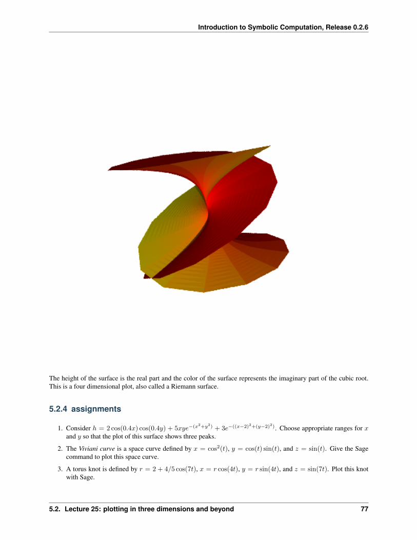
Introduction to Symbolic Computation, Release 0.2.6
The height of the surface is the real part and the color of the surface represents the imaginary part of the cubic root.This is a four dimensional plot, also called a Riemann surface.
5.2.4 assignments
1. Consider ℎ = 2 cos(0.4𝑥) cos(0.4𝑦) + 5𝑥𝑦𝑒−(𝑥2+𝑦2) + 3𝑒−((𝑥−2)2+(𝑦−2)2). Choose appropriate ranges for 𝑥and 𝑦 so that the plot of this surface shows three peaks.
2. The Viviani curve is a space curve defined by 𝑥 = cos2(𝑡), 𝑦 = cos(𝑡) sin(𝑡), and 𝑧 = sin(𝑡). Give the Sagecommand to plot this space curve.
3. A torus knot is defined by 𝑟 = 2 + 4/5 cos(7𝑡), 𝑥 = 𝑟 cos(4𝑡), 𝑦 = 𝑟 sin(4𝑡), and 𝑧 = sin(7𝑡). Plot this knotwith Sage.
5.2. Lecture 25: plotting in three dimensions and beyond 77

Introduction to Symbolic Computation, Release 0.2.6
5.3 Lecture 26: animations
An animation is defined by a list of plots, which will make the frames of the movie. We will show various examplesof animations with the several plotting commands we have covered so far.
As in the previous lecture, our browser is google chrome and we use the Sage Math Cloud.
5.3.1 animating plots
Recall how we started the lecture on two dimensional plots.
t = var('t')f = exp(-t^2)*sin(2*pi*t)plot(f, (t, -2, 2))
The argument of the sine function is set so the frequency equals one, for t going from 0 to 1, the argument of sinegoes for 0 to 2*pi. Suppose we want to see the evolution as we increase the frequency from 1 to 10. We can make asequence of plots, which will be the frames in our animation. To test whether we did not make any mistakes in settingup the list of plots, we render the first frame. What we see should be the same as above.
frames = [plot(exp(-t^2)*sin(2*k*pi*t), (t, -2, 2)) for k in range(1,11)]frames[0].show()
And then, we just call the animate on the list of frames.
animate(frames)
That is it!
5.3.2 animating curves
Polar coordinates are well suited to make nice curves.
t = var('t')r = sin(8*t)polar_plot(r, (t, 0, 2*pi))
Now we can imagine an object that makes a trajectory following that curve. We will make 20 frames, dividing therange for t in steps of 2*pi/20. Observe that we cannot give an empty range for t, so we start at 1 instead of 0. Asa check we look at the last frame, which should show the same plot as above.
frames = [polar_plot(r, (t, 0, k*2*pi/20)) for k in range(1, 21)]frames[19].show()
And then again we call animate.
animate(frames)
But now the animation does not look so good. The problem with the previous animation is that the axes for x and ychange. We can fix the ranges of the axes for x and y by setting the values for xmin, xmax for the x-axis and settingthe values ymin and ymax for the y-axis.
animate(frames, xmin=-1, xmax=1, ymin=-1, ymax=1)
78 Chapter 5. Part IV: plotting and solving equations

Introduction to Symbolic Computation, Release 0.2.6
5.3.3 animating surfaces
Let see if we can animate surfaces, rotating a plane. We consider the family 𝑧 = (1− 𝑘/20)𝑥+ 𝑘/20𝑦, for 𝑘 rangingfrom 0 to 20.
x, y = var('x,y')frames = [plot3d((1-k/20)*x + k/20*y, (x,-1,1), (y,-1,1)) \
for k in range(0, 21)]animate(frames, xmin=-1, xmax=1, ymin=-1, ymax=1, zmin=-1, zmax=1)
For 𝑘 = 0 we have 𝑧 = 𝑥 and for 𝑘 = 20 we have 𝑧 = 𝑦.
5.3.4 assignments
1. The neoid is defined by 𝑟 = 𝑎𝑡+ 𝑏 in polar coordinates.
Give the Sage commands to produce an animation of 10 frames, for 𝑎 = 0.2 and for 𝑏 going from 0.1 to 1, andfor 𝑡 = 0 . . . 6𝜋.
2. Make an animation of a spiral, using the formulas 𝑥 = 𝑡 cos(𝑡), 𝑦 = 𝑡 sin(𝑡), and 𝑧 = 𝑡. Let there be 30 framesin your animation, with 𝑡 = 1, 2, . . . , 30𝜋.
3. The Viviani curve is a space curve defined by 𝑥 = 𝑅 cos2(𝑡), 𝑦 = 𝑅 cos(𝑡) sin(𝑡), and 𝑧 = 𝑅 sin(𝑡), where 𝑅 issome parameter.
Make an animation for the curve for 𝑅 going from 1 to 10 (thus using ten frames). Give all Sage commands youuse to make this animation.
5.4 Lecture 27: solving equations
In this lecture we solve equations. We start with solving a polynomial in one variable where the coefficients dependon a parameter. Solving this polynomial symbolically requires the application of solve many times. Our runningexample of a system of polynomial equations is the Apollonius circle problem. A Groebner basis of an ideal in apolynomial ring with lexicographic term order is a triangular basis.
5.4.1 polynomials in one variable
Let us consider a polynomial with a parameter A.
var('A, x')equ = A^2*(x^2+x+1)-A*(2*x-3) - x^2-3*x+2print equ
Now we can solve for x and obtain symbolic expressions in A as solutions.
s = solve(equ, x)print s
Consider the solutions:
[x == -1/2*(A + sqrt(-3*A^2 - 10*A + 17) - 3)/(A - 1),x == -1/2*(A - sqrt(-3*A^2 - 10*A + 17) - 3)/(A - 1)]
5.4. Lecture 27: solving equations 79

Introduction to Symbolic Computation, Release 0.2.6
The solutions were obtained via the quadratic formula. But what if we solved for A?
sA = solve(equ, A)print sA
and we get A == -1 and A == (x^2 + 3*x - 2)/(x^2 + x + 1) as solutions. Could A = -1 be a spe-cial parameter?
print equ.subs(A=-1)
We see 0 and thus, yes, indeed: A = -1 is a special parameter. We just saw that the equation vanishes when A is setto -1. This means that any value for x is a solution. Could there be other special values for A? What happens whenwe plug in A = 1 in the equation?
equA1 = equ.subs(A = 1)print equA1
When plug in A = 1 we get -4*x + 6. Recall the factor A - 1 in the general solution we first computed. So forA = 1, the solutions we computed before in s are not valid, but there is still a solution, just one single solution.
print solve(equA1, x)
and that solution is x == (3/2). Another way we could have detected the special values for A is via the leadingcoefficient of x in the equation equ.
q = equ.coefficient(x,2)print q
Collecting the terms in x^2 gives A^2 - 1 So the values that kill the leading coefficient of equ are
print solve(q, A)
which of course gives A == -1 and A == 1. But then why does one parameter give such different behaviour forthe solution x than the other? Let us look at the linear coefficient of the equation in x.
q1 = equ.coefficient(x,1)q0 = equ.coefficient(x,0)print q1print q0
and the equations q1 and q0 are respectively A^2 - 2*A - 3 and A^2 + 3*A + 2. Then we solve the expres-sions and we see that A = -1 is a common solution to both the linear and constant coefficient.
print solve(q1, A)print solve(q0, A)
The solutions of q1 are A == 3 and A == -1, while the solutions of q0 are A == -2 and A == -1.
Count the many times we did solve to solve one polynomial equation with parameters and realize that solving equa-tions with parameters symbolically is a much harder problem than solving a polynomial with a numerical coefficients.
5.4.2 solving systems of polynomial equations
We turn our attention to systems of polynomial equations and solve the circle problem of Apollonius: Given threecircles, find all circles that are tangent to the three given circles.
To derive the equations, consider the unit circle and a random circle inside the unit circle. We first plot the unit circle.
80 Chapter 5. Part IV: plotting and solving equations

Introduction to Symbolic Computation, Release 0.2.6
var('x,y')u = x^2 + y^2 - 1p0 = implicit_plot(u, (x, -1, 1), (y, -1, 1))p0.show()
A random circle inside the unit circle has a random center.
cx = RR.random_element(0, 0.5)cy = RR.random_element(0, 0.5)print cx, cyp1 = point((cx, cy), size=50, color='red')(p0 + p1).show()
Now the radius of the circle that touches the unit circle is ...
r = 1 - sqrt(cx^2 + cy^2)print rp2 = implicit_plot((x - cx)^2 + (y - cy)^2 - r^2, (x, -1, 1), (y, -1, 1), \
color='red')(p0 + p1 + p2).show()
We see that there is another solution.
r2 = 1 + sqrt(cx^2 + cy^2)p3 = implicit_plot((x - cx)^2 + (y - cy)^2 - r2^2, (x, -2, 2), (y, -2, 2), \
color='green')(p0 + p1 + p2 + p3).show()
Now we turn our attention to the circle problem of Apollonius. We need three circles on input: The first circle will bethe unit circle. The second circle has center (2, 0) with radius 2/3. The third circle has center (1, 1) with radius 1/3.
(c1x, c1y, r1) = (0, 0, 1)(c2x, c2y, r2) = (2, 0, 2/3)(c3x, c3y, r3) = (1, 1, 1/3)c1 = (x-c1x)^2 + (y-c1y)^2 - r1^2c2 = (x-c2x)^2 + (y-c2y)^2 - r2^2c3 = (x-c3x)^2 + (y-c3y)^2 - r3^2xr = (x, -1, 3); yr = (y, -1, 2)p1 = implicit_plot(c1, xr, yr)p2 = implicit_plot(c2, xr, yr)p3 = implicit_plot(c3, xr, yr)(p1 + p2 + p3).show()
Now we look for the circle that will be tangent to all three circles.
var('r')e1 = (x - c1x)^2 + (y - c1y)^2 - (r - r1)^2e2 = (x - c2x)^2 + (y - c2y)^2 - (r - r2)^2e3 = (x - c3x)^2 + (y - c3y)^2 - (r - r3)^2eqs = [e1, e2, e3]print eqs
and now we solve the system. We set the option solution_dict to True because this works better to select thecoordinates of the solution.
sols = solve(eqs, (x, y, r), solution_dict=True)print sols
5.4. Lecture 27: solving equations 81

Introduction to Symbolic Computation, Release 0.2.6
We see there are two solutions, computed exactly.
s0x = sols[0][x]s0y = sols[0][y]s0r = sols[0][r]print s0x, s0y, s0rsc0 = implicit_plot((x-s0x)^2 + (y-s0y)^2 - s0r^2, (x, -2, 3), (y, -3, 2), \
color='red')s1x = sols[1][x]s1y = sols[1][y]s1r = sols[1][r]print s1x, s1y, s1rsc1 = implicit_plot((x-s1x)^2 + (y-s1y)^2 - s1r^2, (x, -2, 3), (y, -3, 2), \
color='red')(p1 + p2 + p3 + sc0 + sc1).show()
Note that this problem has actually 8 solutions in total. What we computed are only types. Instead of (r-r1), weshould also consider (r+r1).
5.4.3 Groebner bases
We saw that the system was solved exactly, via what looked like the quadratic formula. We will cast the polynomialequations in a polynomial ring with lexicographic order.
PR.<x,y,r> = PolynomialRing(QQ, order='lex')print PRq1 = PR(e1)print q1, type(q1)
We see that PR is a Multivariate Polynomial Ring in x, y, r over Rational Field and thepolynomial q1 has type MPolynomial_libsingular so we will be using the computer algebra system Singular.to work with the polynomials of the Apollonius circle problem. We also cast the other two polynomials into this ringand define the ideal generated by the three polynomials. An ideal generated by polynomials in a ring consists of allcombinations of the generators with elements in the ring.
q2 = PR(e2); q3 = PR(e3)qs = [q1, q2, q3]I = Ideal(qs)print I
A Groebner basis of an ideal in a polynomial ring with lexicographic term order is a triangular basis.
B = I.groebner_basis()print B
The Groebner basis for the ideal generated by the polynomials of the Apollonius circle problem is
[x + 1/6*r - 41/36, y + 1/2*r - 11/36, r^2 - 71/39*r - 253/468]
We see that the last polynomial is a quadratic polynomial in one variable, that is r. Recall that r was the last variablein our lexicographic term order. The other two polynomials are linear and we can express x and y as functions of r.
5.4.4 assignments
1. Consider the polynomial equation 𝑥2𝑎2 − 12𝑥2 + 𝑎2𝑥− 3√3𝑎𝑥+ 6𝑥+ 𝑎2 −
√3𝑎− 6 = 0.
82 Chapter 5. Part IV: plotting and solving equations

Introduction to Symbolic Computation, Release 0.2.6
Give the Sage command to solve the equation with 𝑥 as variable.
For which values of the parameter 𝑎 does the equation have less than two solutions?
Find the solution for this special value of the parameter.
For which values of the parameter 𝑎 does the equation have infinitely many solutions?
Give the Sage commands you used to test your answer.
2. There are eight different solutions to the Apollonius circle problem, which can be obtained by consideringinstead of r - r1 also r + r1 and likewise for the radii r2 and r3. Make a plot that shows all eightdifferent solutions and give all Sage commands to obtain all solutions.
3. Solve the system {𝑥2 + 𝑦2 − 5 = 09𝑥2 + 𝑦2 − 9 = 0
Make a plot of the two algebraic curves to confirm the values found for the intersection points.
How many solutions did you find? How many solutions do you see?
4. As an illustration of the technique of Lagrange multipliers we derived the system in the list below:
[-2*w*x + 2*y*z + 2*x == 0, -2*w*y + 2*x*z == 0,2*x*y - 2*w*z - 2*z == 0, x^2 + y^2 + z^2 - 1 == 0]
Compute a Groebner basis for a ideal generated by the three polynomials in the list above, with a lexicographicterm order.
Explain how you can compute the number of solutions from the triangular structure of the Groebner basis.
5. A comet approaches earth in an ellipsoid path, defined by (𝑥− 2)2/6 + 𝑦2/2− 1 = 0, where the earth is at thecenter (0, 0) of our coordinate system.
We want to know the locations where the comet is closest to earth.
(a) Set up the polynomial system to find those locations.
(b) Solve the polynomial system and find the coordinates on the ellipse closest to the origin.
(c) Make a plot of the ellipse and the solution found in (b).
5.5 Lecture 28: linear algebra
In this lecture we do linear algebra: we solve linear equations. The formalism to describe linear equations is viamatrices. Let us first then look at the matrix types.
5.5.1 matrices and linear systems
With the data in a list of lists, we can make a matrix.
A = Matrix(ZZ,[[1,2],[3,4]])print A, type(A)
Some matrices are defined by formulas. For example, let us make a 3-by-4 integer matrix where the (𝑖, 𝑗)-th entry is1
𝑖+𝑗 , for 𝑖 and 𝑗 both going from 1 to 𝑛. Let us make a 3-by-4 matrix with this formula.
5.5. Lecture 28: linear algebra 83

Introduction to Symbolic Computation, Release 0.2.6
B = Matrix(QQ, 3, 4, lambda i,j: 1/((i+1)+(j+1)))print B
Observe that we had to change the formula because in Python as in Sage we count from zero and we do not want 1/0as the first element in the first row.
We can make a random matrix that way.
C = Matrix(ZZ, 3, 3, lambda i,j: randint(0,10))print C
We can make a random matrix over the rational numbers. In the example below we bound the size of numerator anddenominator by 100.
D = random_matrix(QQ, 4, num_bound=100, den_bound=100)print D
A random vector can be made just as easily.
v = random_vector(QQ, 4)print v, type(v)
We can solve linear systems with the backslash operator (as in MATLAB).
x = D\vprint xprint D*x
We thus solved with x = A\b the linear system A*x = v.
5.5.2 matrices over fields
One way to solve linear systems is via a LU factorization. An LU factorization writes the matrix as a product of alower with an upper triangular matrix.
A = random_matrix(QQ, 4, num_bound=100, den_bound=100)print 'A =\n', AP, L, U = A.LU()print 'L =\n', Lprint 'U =\n', Uprint 'P =\n', Pprint 'P*L*U =\n', P*L*Uprint 'A =\n', A
How does the LU factorization relate to solving linear systems? Well, because A = P*L*U, the system A*x = bbecomes P*L*(U*x) = b, or if we set y = U*x, then we first solve P*L*y = b and then solve U*x = y. Letus try if that works on the example, for a random b.
b = random_vector(QQ, 4)PL = P*Ly = PL\bx = U\yprint xprint A\b
We see that x and A\b show the same vector.
84 Chapter 5. Part IV: plotting and solving equations

Introduction to Symbolic Computation, Release 0.2.6
Another important decomposition is the eigenvector-eigenvalue decomposition, which for general matrices, diagonal-izes the matrix.
A = random_matrix(QQ, 4, 4)print 'A =\n', Ae = A.eigenvalues()print 'the eigenvalues :\n', e
We see that the eigenvalues seem numerical:
print type(e[0])
but they are of type sage.rings.qqbar.AlgebraicNumber. The eigenvalues are roots of a polynomial, thecharacteristic polynomial of the matrix A.
p = A.charpoly()print pprint p.roots(QQbar)print p.roots(CC)
For an eigenvector z of a matrix with eigenvalue L, we have A*z = L*z. Let us verify this property for the firsteigenvalue and eigenvector. The eigenvectors are stored in the columns of the matrix P.
D, P = A.right_eigenmatrix()
Let us verify the relations between the matrices.
print 'D =\n', Dprint 'the eigenvectors :\n', Pprint 'P*D =\n', P*Dprint 'A*P =\n', A*P
We have that A*P = P*D, where D is a diagonal matrix. Since P is invertible, we have D = P^(-1)*A*P.
p1ap = P.inverse()*A*Pprint p1apprint Dprint D-p1ap
The last output is the matrix of very small numbers.
For an eigenvector z of a matrix with eigenvalue L, we have A*z = L*z. Let us verify this property for the firsteigenvalue and eigenvector. The eigenvectors are stored in the columns of the matrix P.
v = P[:,0]print vAv = A*vDv = D[0,0]*vprint Avprint Dv
We see that both vectors Av and Dv are the same.
5.5.3 matrices over rings
Recall that in a ring we cannot divide. We can then still solve linear systems with fraction-free row reduction.
5.5. Lecture 28: linear algebra 85

Introduction to Symbolic Computation, Release 0.2.6
The Hermite normal form H of a matrix A is an upper triangular form obtained by multiplying A with a unimodulartransformation U. A unimodular matrix U has determinant 1 or -1.
A = Matrix(ZZ, 4, 4, lambda i,j: randint(1,10))print 'A =\n', AH, U = A.hermite_form(transformation=True)print 'H =\n', Hprint 'U =\n', Uprint 'U*A =\n', U*A
We can check the determinants via the det() method.
print 'det(A) =', A.det()print 'det(U) =', U.det()print 'det(H) =', H.det()
We see that det(U*A) = det(U)*det(A).
The Hermite normal form is a triangular matrix. The Smith normal form is a diagonal matrix. In addition to thediagonal matrix D, the smith_form() method returns two unimodular matrices U and V.
D, U, V = A.smith_form()print 'D =\n', Dprint 'U =\n', Uprint 'V =\n', Vprint 'U*A*V =\n', U*A*V
5.5.4 resultants
With a lexicographic Groebner basis we can eliminate variables and obtain a triangular form of the system. Analternative construction is to use resultants, which are available via Singular. We use Singular when we declare apolynomial ring.
PR.<x,y> = PolynomialRing(QQ)print PRp = x^2 + y^2 - 5q = 9*x^2 + y^2 - 9print type(p), type(q)
We see that PR is then a Multivariate Polynomial Ring in x, y over Rational Field and bothp and q are of type MPolynomial_libsingular.
Now we can eliminate one of the variables, say x. We eliminate from p the variable xwith respect to q, or equivalently,we eliminate from q the variable x with respect to p.
print p.resultant(q,x)print q.resultant(p,x)
We see the same polynomial 64*y^4 - 576*y^2 + 1296 twice. Similarly, we can eliminate y via p.resultant(q,y) and q.resultant(p,y). With the resultant we can thus compute the coordinates of theroots.
Resultants are determinants of the so-called Sylvester matrix.
sp = p.sylvester_matrix(q, x)print spprint sp.det()
86 Chapter 5. Part IV: plotting and solving equations

Introduction to Symbolic Computation, Release 0.2.6
The output of sp.det() corresponds to p.resultant(q, y).
5.5.5 assignments
1. The (𝑖, 𝑗)-th entry in an n-by-n Vandermonde matrix is defined as 𝑥𝑗−1𝑖 , for i and j both ranging from 1 to n.
Give the Sage command(s) to make a 4-by-4 Vandermonde matrix.
2. Compute the determinant of a 4-by-4 Vandermonde matrix (see the previous exercise). Show that it factors asthe product of all differences (𝑥𝑖 − 𝑥𝑗) for 𝑗 > 𝑖 and all i from 1 to 4.
3. Given a polynomial p in one variable, the companion matrix of p as eigenvalues the roots of p. We will verifythis property on a random polynomial.
(a) Generate a monic random polynomial p of degree five. A monic polynomial has its leading coefficientequal to one. Use the Sage command companion_matrix (look up the help page on its use) to generatethe companion matrix of p.
(b) Compute the eigenvalues of the companion matrix and compare the eigenvalues with the output of p.roots(CC).
4. The (𝑖, 𝑗)-th entry of an 𝑛-by-𝑛 Lehmer matrix ismin(𝑖, 𝑗)
max(𝑖, 𝑗), for 𝑖 and 𝑗 both ranging from 1 to 𝑛.
Generate a 5-by-5 Lehmer matrix and verify that all its eigenvalues are positive.
5.6 Lecture 29: solving differential equations
In Sage, differential equations can be solved with desolve. As the help(desolve) shows, the desolve solvesfirst or second order linear ordinary differential equations via the computer algebra system maxima.
We distinguish between initial value and boundary value problems. The pendulum problem is an example of an initialvalue problem, the heat diffusion problem is an example of a boundary value problem.
5.6.1 the pendulum problem
As our running example of a differential equation, consider a pendulum. We have a mass attached to a string, subjectto gravity. The variable is theta(t), the angle of deviation from the vertical position of the string, as a function intime.
var('t')theta = function('theta', t)print theta
In the formulation of the Ordinary Differential Equation (ODE), the gravitational constant is denoted by g, and L isthe length of the string. Applying Newton’s laws leads to an equation of second order, involving the second deriva-tive. A more geometrically precise model would have -g*sin(theta), but for small angles theta we simplifysin(theta) to theta.
var('g, L')ode = L*diff(theta,t,2) == -g*thetaprint ode
The command to solve a differential equation is desolve. We have to tell desolvewhat is the independent variable,given below in the argument ivar = t.
5.6. Lecture 29: solving differential equations 87

Introduction to Symbolic Computation, Release 0.2.6
sol = desolve(ode, theta, ivar=t)print sol
The desolve throws an exception. The computation failed since Maxima requested additional constraints. Sageasks: Is g*L positive, negative or zero? With knowing the signs of the gravitational constant g or thelength L of the string, we cannot solve the problem, but of course, g and L are both positive.
assume(g > 0, L > 0)sol = desolve(ode, theta, ivar=t)print sol
The answer we get is
_K2*cos(sqrt(g)*t/sqrt(L)) + _K1*sin(sqrt(g)*t/sqrt(L))
The _K1 and _K2 in the expression for the solution are general constants. We have two degrees of freedom, asexpected for a second order equation. We can formulate an Initial Value Problem. As initial conditions, we assumethat we move the mass to an angle of pi/10, with velocity zero. Suppose that at t = 0, we have an initial angle ofpi/10, thus: theta(0) = pi/10 and its derivative is 0, so we have D[0](theta)(0) = 0.
sol = desolve(ode, theta, ivar=t, ics=[0, pi/10, 0])print sol
and we see 1/10*pi*cos(sqrt(g)*t/sqrt(L)) as a general symbolic solution to the initial value problem.To plot the solution, we supply values for the gravitational constant g and the length of the string L.
s = sol.subs(g=10, L=3)print splot(s, (t, 0, 2*pi))
5.6.2 heat diffusion
As an example of a boundary value problem, consider the diffusion of heat in a rod. We have a rod of length one.The rod experiences temperature differences at its ends. We are interested in the equilibrium temperature distribution,which in its simplest form is expressed as a second order differential equation.
var('x')u = function('u', x)ode = diff(u, x, 2) == 0print ode
As boundary conditions we impose u(0) = 2.5 and u(1) = 3.1.
sol = desolve(ode,u, ivar= x, ics=[0, 2.5, 1, 3.1])print sol
and we find as solution 3/5*x + 5/2.
5.6.3 assignments
1. Solve the following initial value problem:
𝑦′′ − 𝑦 = 0, 𝑦(0) = 1, 𝑦′(0) = 0.
Note that 𝑦′ denotes the first derivative and 𝑦′′ the second derivative with respect to some independent variable.
88 Chapter 5. Part IV: plotting and solving equations

Introduction to Symbolic Computation, Release 0.2.6
5.7 Lecture 30: Polyhedra and Linear Programming
5.7.1 polyhedra
A convex combination of two points is the line segment that has the two points as its ends. Given a set of points, theconvex hull of the point is the set of all convex combinations of the points. For points in the plane, this convex hull isa polygon. We can draw a polygon by giving the vertices (or corner points).
P = polygon([(0,0), (1,0), (2,1)])P.show()
The edges of the polygon are three line segments, we call them A, B, and C, and they are spanned by the points in thelists e1, e2, and e3.
e1 = [(0,0), (1,0)]e2 = [(1,0), (2,1)]e3 = [(2,1), (0,0)]A = polygon(e1, thickness=3, color='red')B = polygon(e2, thickness=3, color='green')C = polygon(e3, thickness=3, color='yellow')(A + B + C).show()
We can define a polygon as the intersection of halfspaces, defined by the lines along the edges of the polygon.
AL = line(e1, thickness=3)BL = line(e2, thickness=3)CL = line(e3, thickness=3)(AL+BL+CL).show(axes=False)
5.7.2 linear programming
Linear programming optimizes linear functions subject to linear constraints. The following example of a linear pro-gram is taken from the Sage documentation.
max𝑥+ 5𝑦subject to{
𝑥+ 0.2𝑦 ≤ 41.5𝑥+ 3𝑦 ≤ 4
where the variables 𝑥 and 𝑦 are both real and positive. In Sage this can be solved as follows:
p = MixedIntegerLinearProgram(maximization=True)x = p.new_variable(nonnegative=True)p.set_objective(x[1] + 5*x[2])p.add_constraint(x[1] + 0.2*x[2], max=4)p.add_constraint(1.5*x[1] + 3*x[2], max=4)p.solve()
and we see 6.666666666666666 as the solution.
Let us look at this problem a bit in greater detail.
A = ([1, 0.2], [1.5, 3])b = (4, 4)c = (1, 5)
5.7. Lecture 30: Polyhedra and Linear Programming 89

Introduction to Symbolic Computation, Release 0.2.6
P = InteractiveLPProblem(A, b, c, ["x1", "x2"], problem_type="max", \constraint_type="<=", variable_type=">=")
P.plot()
The output of the run_simplex_method() is LaTeX code. To see it typeset properly, we must check the typesetbox in a Sage worksheet. We first convert the problem to its standard form.
P = P.standard_form()P.run_simplex_method()
The interactive run of the simplex method shows the succession of dictionaries.
5.7.3 unconstrained minimization
We covered the technique of Lagrange multipliers already to solve a constrained optimization problem. As an examplewe take a sum of squares.
var('x,y')f(x,y) = (3+x-y^2)^2 + (x - 1)^2 + (y - 1)^2pf = plot3d(f(x,y), (x, -2, 3), (y, -2, 3), adaptive=True, color='automatic',→˓opacity=0.5)pf.show()
We can look for a minimum. We need to give an initial guess.
p = minimize(f, x0=[0.0, 0.0])print 'minimum at', p, 'with value', f(p[0], p[1])
Then Sage prints
Optimization terminated successfully.Current function value: 0.882789Iterations: 10Function evaluations: 14Gradient evaluations: 14
minimum at (0.766044177107, 1.87938504258) with value 0.882788808286
To get an idea how good this minimum is we take a look at where the location on the minimum on the surface.
pt = point((p[0], p[1], f(p[0],p[1])), size=10, color='red')(pt+pf).show()
5.7.4 assignments
1. Suppose General Motors makes a profit of $100 on each Chevrolet, $200 on each Buick, and $400 on eachCadillac. These cars get 20, 17, and 14 miles a gallon respectively, and it takes respectively 1, 2, and 3 minutesto assemble one Chevrolet, one Buick, and one Cadillac. Assume the company is mandated by the governmentthat the average car has a fuel efficiency of at least 18 miles a gallon. Under these constraints, determine theoptimal number of cars, maximizing the profit, which can be assembled in one 8-hour day. Give all Sagecommands and the final result.
2. Take the gradient of f(x,y) = (3+x-y^2)^2 + (x - 1)^2 + (y - 1)^2 and solve the polyno-mial system defined by setting the gradient to zero. The solutions of this system contain the minima of thefunction. Do you find the outcome of minimize among the solutions of the system?
90 Chapter 5. Part IV: plotting and solving equations

Introduction to Symbolic Computation, Release 0.2.6
5.8 Lecture 31: review of lectures 17 to 30
Below is a first, preliminary list of equations to review in preparation of the second midterm exam. Consider also thequizzes and homework assignments.
1. Count the number of points with integer coordinates (𝑥, 𝑦), in the region defined by the inequalities 0 ≤ 𝑥 < 20,0 ≤ 𝑦 < 20, 𝑦 ≥ 𝑥/2, and 𝑦 ≤ 3𝑥. Give the Sage commands (not the output) for the three stages below.
(a) Generate a list 𝐿 of integer points (𝑖, 𝑗) for 𝑖 and 𝑗 ranging between 0 and 19.
(b) Select from the list 𝐿 those points in the cone 𝑦 ≥ 𝑥/2 and by 𝑦 ≤ 3𝑥.
(c) Count the number of points in the cone. Write also the number below.
2. For some parameter 𝑡, consider the sequence recursively defined as:
𝐹𝑛 = (1− 𝑡)𝐹𝑛−1 + 𝑡𝐹𝑛−2, for 𝑛 > 1,
where 𝐹 (0) = 𝑎 and 𝐹 (1) = 𝑏. Using the recursive definition write an efficient Sage function 𝐹 to compute 𝐹𝑛
as F(a, b, t, n). What is the result of F(a, b, 0.3, 100)?
3. Consider the function 𝑓(𝑡) =
∫ 𝑡
0
(1− 𝑒𝑥)𝑑𝑥, for 𝑡 ≥ 0. Define this function in Sage. What is 𝑓 ′(1)?
4. The function 𝑔(𝑥, 𝑡) =1− 𝑡2
1− 2𝑥𝑡+ 𝑡2is a generating function for the Chebyshev polynomials. Compute a Taylor
series approximation for 𝑔(𝑥, 𝑡) around 𝑡 = 0 of order 10. Select the coefficient of 𝑡8 and compare with theoutput of chebyshev_T(8, x). Is there a difference between the two?
5. Consider the point (1, 1) on the curve 𝑓(𝑥, 𝑦) = 𝑥2 − 𝑦3 − 𝑥+ 𝑦 = 0.
(a) Give the Sage command(s) to compute a Taylor series about the point (1, 1) where the term of the error isof second order.
(b) Compute the slope of the tangent line of the curve at the point (1, 1) and use the slope to determine thetangent line. Write the equation of the tangent line.
Verify that the equation for the tangent line corresponds to the first-order Taylor series at (1, 1).
6. Consider the curve 𝑥4 − 3𝑥𝑦 + 𝑦4 = 0. Give all Sage commands to
(a) to make a plot for 𝑥 and 𝑦 both ranging between −2 and +2;
(b) to convert the curve into polar coordinates; and
(c) to plot the curve in polar coordinates.
7. Consider 𝑝 = 5𝑥2𝑎2 + 61𝑥2𝑎 + 66𝑥2 + 10𝑥𝑎2 + 121𝑥𝑎 + 121𝑥 + 𝑎2 + 15𝑎 + 44, as a polynomial in 𝑥 withparameter 𝑎.
(a) Find the roots of 𝑝.
(b) For which values of the parameter 𝑎 is the answer valid?
(c) Give the Sage command(s) to treat the special case(s).
(d) As you can see the polynomial 𝑝 is shown in expanded form. Give the Sage command(s) to ‘’un-expand’‘,i.e.: what is the command which reveals better the structure of 𝑝?
8. Let 𝑎 and 𝑏 be positive numbers. Consider 𝑓 = 𝑥2/𝑎 + 𝑦/𝑏 and the unit circle 𝑥2 + 𝑦2 = 1. Give all Sagecommands to determine the number of candidate extremal values of 𝑓 on the unit circle. Use a lexicographicGroebner basis to compute a triangular form of the equations for this problem.
5.8. Lecture 31: review of lectures 17 to 30 91

Introduction to Symbolic Computation, Release 0.2.6
9. Give the Sage commands for the following tasks. Create a 5-by-5 matrix 𝐴 over the rationals where the (𝑖, 𝑗)-theelement is 1/𝑖 + 𝑗 (for 𝑖 and 𝑗 both from 1 to 5). Define b as a vector of length 5 of ones. Solve the systemdefined by 𝐴𝑥 = 𝑏. Verify that 𝑏−𝐴𝑥 equals zero.
5.9 Lecture 32: second midterm exam
The second midterm exam covers parts three and four of the course.
92 Chapter 5. Part IV: plotting and solving equations

CHAPTER 6
Part Five : advanced Sage
The goal of this part is to look more how Sage connects to other software packages and to cover some advanced topics,or deepen our knowledge about earlier issues. We start with making interactive web pages. Then we cover sympy,numpy, and scipy. The last lecture are spent on Maxima, GAP, PARI/GP, Singular, and R.
6.1 Lecture 33: building interactive web pages
We can view an interactive web page as a graphical user interface, with the main difference that we need a browser torun the interaction.
At UIC, the computer people.uic.edu offers web hosting to students, staff and faculty. If Apache runs on yourcomputer, then you can run the web pages by pointing your browser to localhost.
We follow chapter 6 in the book of Gregory Bard and work through the tangent-line interact.
6.1.1 drawing tangent lines to a curve
The code below is adapted from Sage for Undergraduates by Gregory Bard, pages 285 in Figure 1.
f(x) = x^3 - xdf(x) = diff(f(x), x)def tangent_at_point(x0):
"""Shows the tangent line at the point x0,using f and its derivative as global variables."""y0 = f(x0)slope = df(x0)# y - y0 = slope*(x - x0) implies# y = slope*x - slope*x0 + y0b = y0 - slope*x0P1 = plot(f, -2, 2, color='blue', ymin=-6, ymax=6, gridlines='minor')P2 = plot(slope*x + b, -2, 2, color='tan', ymin=-6, ymax=6)
93

Introduction to Symbolic Computation, Release 0.2.6
P3 = point((x0, y0), color='red', size=50)P = P1+P2+P3P.show(figsize=3)
To test the script we run the following cases in separate cells.
tangent_at_point(0.5)tangent_at_point(1.5)tangent_at_point(-1.75)
We want to attach a scale to the x0 parameter of the function. When the user then moves the scale, the point on thecurve will move and the tangent line at that new point will be shown. To the code we add @interact before thefunction definition. In the header of the function we add the slider.
The parameter x0 of the function is extended into x0 = slider(-2, 2, 0.1, -1.5,label='x-coordinate'). The first two arguments, -2 and 2 determine the range of the slider, so x0 isconstrained to take values in the interval with bounds -2 and 2. The granularity of the slider is defined as 0.1, thethird parameter of the slider(). The fourth parameter sets the initial value -1.5 of x0.
f(x) = x^3 - xdf(x) = diff(f(x), x)@interactdef tangent_at_point(x0 = slider(-2, 2, 0.1, -1.5, label='x-coordinate')):
"""Shows the tangent line at the point x0,using f and its derivative as global variables."""y0 = f(x0)slope = df(x0)# y - y0 = slope*(x - x0) implies# y = slope*x - slope*x0 + y0b = y0 - slope*x0P1 = plot(f, -2, 2, color='blue', ymin=-6, ymax=6, gridlines='minor')P2 = plot(slope*x + b, -2, 2, color='tan', ymin=-6, ymax=6)P3 = point((x0, y0), color='red', size=50)P = P1+P2+P3P.show()
If we execute the code in the cell, then we can already test the interact as it would run in a web page.
6.1.2 making the web page
On page 294 of Sage for Undergraduates by Gregory Bard, we have a template of a web page, based on work of JasonGrout. Once we insert the code in the last cell of the previous section, we are ready to publish the interactive webpage.
6.1.3 drop down menu
With selector we add a drop down menu to let the user choose from a range of options. For example, to select acolor.
fun = x^3 - xrng = (x, -2, 2)@interactdef colorplot(colrgb=selector(['red', 'green', 'blue'], label='color: ')):
94 Chapter 6. Part Five : advanced Sage

Introduction to Symbolic Computation, Release 0.2.6
"""Plots the expression defined by fun over the range in rng.The parameters fun and rng must be defined before calling colorplot.The user can select the color."""P = plot(fun, rng, color=colrgb)P.show()
6.1.4 assignments
1. Consider the function 𝑓(𝑥) = exp(−𝑥2) sin(2𝑘𝜋𝑥) for 𝑥 ∈ [−2,+2] and for 𝑘 ranging from 1 to 10. Make aninteractive web page that plots 𝑓(𝑥) and with a slider so the user can set 𝑘.
2. When plotting in three dimensions we can rotate the axes, for example with the rotateX method. Make aninteractive plot3d method where the argument for rotateX can be manipulated with a slider.
6.2 Lecture 34: an application of interact
In this lecture we consider an application of interact. We build a model of a four bar mechanism. The mechanismis attributed to Chebyshev and it transmits straight to circular motion. We build the interact in three stages, first thecrank, then we solve a polynomial system to determine the coordinates of the connector point. In the third stage weadd the coupler point and the fourth bar.
To learn more about the Chebyshev mechanism, see for example Kinematics, Dynamics, and Design of Machinery byKenneth J. Waldron and Gary L. Kinzel, second edition, John Wiley & Sons, 2003.
6.2.1 turning a crank
Let us start with the making of an interact for a crank. The parameter in the slider is an angle, which ranges from0 to 2*pi, with increments of 0.1, starting a zero. Each time the user touches the slider, the line between (0,0) and(cos(angle), sin(angle)) is drawn.
@interactdef show_crank(angle = slider(0, 2*pi, 0.1, 0, label='angle')):
"""Shows the drawing of a crank, where the user can slide the angleto turn the crank."""center = (0,0)endpnt = (cos(angle), sin(angle))pltcnt = point(center, size=50)pltend = point(endpnt, size=50)crank = line([center, endpnt])(pltcnt+crank+pltend).show(xmin=-1, xmax=1, ymin=-1, ymax=+1)
Observe the ranges for x and y in the show().
6.2.2 computing coordinates of the connector point
There is a bar connected to the end point of the crank. The end point of that bar is connected to another bar, of length5/2, that originates at (2,0). To find the coordinates of the connector point, we intersect two circles.
6.2. Lecture 34: an application of interact 95
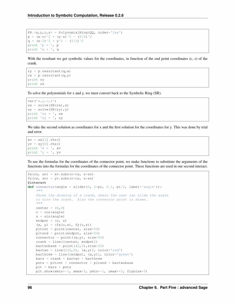
Introduction to Symbolic Computation, Release 0.2.6
PR.<x,y,c,s> = PolynomialRing(QQ, order='lex')p = (x-c)^2 + (y-s)^2 - (5/2)^2q = (x-2)^2 + y^2 - (5/2)^2print 'p = ', pprint 'q = ', q
With the resultant we get symbolic values for the coordinates, in function of the end point coordinates (c, s) of thecrank.
ry = p.resultant(q,x)rx = p.resultant(q,y)print ryprint rx
To solve the polynomials for x and y, we must convert back to the Symbolic Ring (SR).
var('x,y,c,s')sx = solve(SR(rx),x)sy = solve(SR(ry),y)print 'sx = ', sxprint 'sy = ', sy
We take the second solution as coordinates for x and the first solution for the coordinates for y. This was done by trialand error.
xv = sx[1].rhs()yv = sy[0].rhs()print 'x = ', xvprint 'y = ', yv
To use the formulas for the coordinates of the connector point, we make functions to substitute the arguments of thefunctions into the formulas for the coordinates of the connector point. These functions are used in our second interact.
fx(cs, sn) = xv.subs(c=cs, s=sn)fy(cs, sn) = yv.subs(c=cs, s=sn)@interactdef connector(angle = slider(0, 2*pi, 0.1, pi/2, label='angle')):
"""Shows the drawing of a crank, where the user can slide the angleto turn the crank. Also the connector point is drawn."""center = (0,0)c = cos(angle)s = sin(angle)endpnt = (c, s)(x, y) = (fx(c,s), fy(c,s))pltcnt = point(center, size=50)pltend = point(endpnt, size=50)connector = point((x,y), size=50)crank = line([center, endpnt])bartwobase = point((2,0),size=50)bartwo = line([(2,0), (x,y)], color='red')barthree = line([endpnt, (x,y)], color='green')bars = crank + bartwo + barthreepnts = pltcnt + connector + pltend + bartwobaseplt = bars + pntsplt.show(xmin=-1, xmax=3, ymin=-1, ymax=+3, figsize=3)
96 Chapter 6. Part Five : advanced Sage

Introduction to Symbolic Computation, Release 0.2.6
6.2.3 adding the coupler and fourth bar
The final addition is the coupler point and the fourth bar. The fourth bar lies in the extension of the end point of thecrank and the connector point. As the fourth bar has the same length as the bar between the end point of the crank andthe connector point, to obtain the coordinates of the coupler point, we add the differences between connector and endpoint of the crank to the coordinates of the connector point.
@interactdef coupler(angle = slider(0, 2*pi, 0.1, pi/2, label='angle')):
"""Shows the drawing of a crank, where the user can slide the angleto turn the crank. Also the connector point is drawn,with the coupler point and fourth bar."""center = (0,0)c = cos(angle)s = sin(angle)endpnt = (c, s)(x, y) = (fx(c,s), fy(c,s))dx = x - cdy = y - sxx = x + dxyy = y + dypltcnt = point(center, size=50)pltend = point(endpnt, size=50)connector = point((x,y), size=50)coupler = point((xx,yy), size=50, color='red')crank = line([center, endpnt])bartwobase = point((2,0),size=50)bartwo = line([(2,0), (x,y)], color='red')barthree = line([endpnt, (x,y)], color='green')barfour = line([(x,y), (xx,yy)], color='blue')bars = crank + bartwo + barthree + barfourpnts = pltcnt + connector + pltend + bartwobase + couplerplt = bars + pntsplt.show(xmin=-1, xmax=5, ymin=-1, ymax=+5, figsize=5)
As we move the crank, we see that the coupler point traces a straight line. Thus the mechanism translates the rotationalmotion of the crank to the straight motion of the coupler point.
6.2.4 deploying the interactive web page
When we insert the code into a web page, we must ensure that the entire context is defined. For this application, thismeans that we declare the variables c and s, and also define the formulas xv and yv.
6.2.5 assignments
1. Add an extra parameter to the interact that shows the crank. The extra parameter is the length L of the crank, sothe end point has coordinates (L*cos(angle), L*sin(angle)).
2. As a continuation of the previous exercise, find the coordinates of the connector point, symbolically in functionof the variables c, s, and L.
3. Still as a continuation of the previous exercises, extend the interact of the connector with an extra slider for thelength of the crank.
6.2. Lecture 34: an application of interact 97

Introduction to Symbolic Computation, Release 0.2.6
4. Finally, extend the interact of the coupler point with a slider for the length of the crank.
5. Extend the interact of the coupler point so that the path of the coupler point is drawn with a list_plot for theangle going from zero till the position determined by the current value of the angle.
6.3 Lecture 35: symbolic computation with sympy
SymPy is pure Python package for symbolic computation. The pure means that, unlike in Sage, no modifications tothe Python scripting language have been made. SymPy is integrated in Sage and at times we need to be aware of howto use its functionality properly.
6.3.1 sympy outside Sage
Outside Sage, we can compute with SymPy as in the Sage cell server, point your browser to the URL <http://live.sympy.org>.
A comparison of SymPy versus Sage is given at <https://github.com/sympy/sympy/wiki/SymPy-vs.-Sage>.
SymPy is one of the core packages of the SciPy stack <http://www.scipy.org>.
6.3.2 sympy inside Sage
We explicitly applied sympy to define a generator for the terms in a Taylor series.
If we use sympy in Sage, then we may have to be explicit about the use of its functions. For example, the var in Sageis different from the var in sympy.
import sympysympy.var('x')print type(x)
We see that the type of x is sympy.core.symbol.Symbol.
Observe the difference with the var that we are normally using in Sage:
var('y')print type(y)
and the type is sage.symbolic.expression.Expression.
If we use the sqrt() on a variable that is a sympy symbol, then we get a symbolic expression of Sage on return.
print type(sqrt(x))print type(sqrt(y))
In both cases we see the same type. We can make a generator object on the sqrt(1-x). That works.
tsqrtx = sympy.series(sqrt(1-x),x,0,n=None)print tsqrtxprint [tsqrtx.next() for k in range(10)]
But it will not work on sqrt(1-y).
tsqrty = sympy.series(sqrt(1-y),y,0,n=None)print tsqrtyprint [tsqrty.next() for k in range(10)]
98 Chapter 6. Part Five : advanced Sage
Introduction to Symbolic Computation, Release 0.2.6
Although tsqrty is also some type of generator, the application of the generator triggers an exception.
So for the generating function for the Catalan numbers, we must use a sympy symbol x and not a Sage variable y.
g = (1 - sqrt(1-4*x))/(2*x)cg = sympy.series(g,x,0,n=None)print [cg.next() for k in range(11)]print catalan_number(10)
Another feature that is a bit better in SymPy than in Sage is pattern matching, which can be useful when combinedwith substitution. To run this code we can also open a Terminal session, select Misc, and select python.
reset()from sympy import *x = Symbol('x')y = Wild('y')d = (10*x**3).match(y*x**3)print d
On return is a dictionary that has y_ as key with 10 as corresponding value.
6.3.3 assignment
1. What happens if you ask Sage or sympy to compute a Taylor series expansion of sqrt(x) at x = 0? Explainthe result.
6.4 Lecture 36: numerical computation with numpy and scipy
Many problems in scientific computing reduce to numerical linear algebra and numerical algorithms to solve dif-ferential equations. The packages numpy and scipy are standalone packages for use with Python and they are partof the core packages in the SciPy stack, see <http://www.scipy.org>. For plotting in Sage, we have Matplotlib,<http://www.matplotlib.org>, which is also part of the SciPy distribution.
Both numpy and scipy are integrated in Sage. The main functionality of numpy is that it extends Python with matricesand multidimensional arrays. The package scipy bundles several standard scientific mathematical libraries. Examplesof such libraries are BLAS and LAPACK for numerical linear algebra, QUADPACK for numerical integration, andODEPACK for the numerical solution of ordinary differential equations.
6.4.1 numpy
We have been using numpy already in our plotting.
from sage.misc.citation import get_systemsget_systems("point([0,0], size=50).show(figsize=1, axes=False)")
From the output ['numpy'] we see that numpy is credited with the display of the point.
To visualize large data sets, we can use matrix_plot.
import numpy as npA = np.random.normal(0, 1, (20, 20))matrix_plot(A, cmap='hsv', colorbar=True)
6.4. Lecture 36: numerical computation with numpy and scipy 99

Introduction to Symbolic Computation, Release 0.2.6
We have already a random coefficient matrix A. Let us generate a random right hand side vector b and solve a linearsystem A*x = b. The random numbers are uniformly distributed in the interval [-1,+1].
b = np.random.uniform(-1, 1, (20, 1))x = np.linalg.solve(A, b)v = b - A*xr = np.linalg.norm(v)print r
What we see printed as the value of r is 18.1786344846. The residual r of a linear system is the norm of b -A*x, but something went wrong, because the residual is too large! What is the problem? Let us look at the type of A,b, and x.
print 'type(A) :', type(A)print 'type(b) :', type(b)print 'type(x) :', type(x)
In all three cases, we see numpy.ndarray as the type. For the operator arithmetic to work properly, we must convertto the proper matrix types.
mA = np.matrix(A)print type(mA)mb = np.matrix(b)print type(mb)mx = np.matrix(x)print type(mx)
The variables mA, mb, and mx are instances of the class numpy.matrixlib.defmatrix.matrix. Now we cancompute the residual correctly.
v = mb - mA*mxr = np.linalg.norm(v)print r
As we see for the value of r the number 2.37857348102e-15 we see that the solution x of the linear system A*x= b is accurate within the machine precision for hardware doubles.
The fundamental data type in a MATrix LABoratory is a matrix and numpy gives matrices to Python. Vectorization isa technique to formulate linear algebra operations with vector and matrix arithmetic. The arithmetic is performed ondedicated data structures by optimized and fine tuned libraries.
6.4.2 scipy
Many expressions do not have symbolic antiderivatives.
f = exp(sin(x))a = integral(f, x, 0, 1)print a
Sage then returns integrate(e^sin(x), x, 0, 1). Then with a.n() we can get a numerical approxima-tion. Sometimes we may directly go for a numerical approximation and apply quadrature rules.
from scipy.integrate import quadd = quad(f, 0, 1, full_output=1)print d
100 Chapter 6. Part Five : advanced Sage

Introduction to Symbolic Computation, Release 0.2.6
Not only is the numerical approximation returned, but also an estimate for the error and the number of functionevaluations.
Often we use a combination of sympy and scipy. For example, the computation of a Padé approximation starts from aTaylor series. We can compute Taylor series with sympy and Padé approximations with scipy.
from sympy import var, sin, seriesvar('x')s = series(sin(x), x, 0, 6)print 'the Taylor series of sin(x) at x = 0 of order 6 :', sc = [s.coeff(x, k) for k in range(6)]print 'the coefficients of the series :', c
The coefficients of the series are [0, 1, 0, -1/6, 0, 1/120]. We import the pade command fromscipy.misc. The first argument of pade is the list with the coefficients of the Taylor series. The second argumentis the degree of the denominator of the rational approximation. So if we want a denominator of degree 2, we proceedas follows.
from scipy.misc import padep = pade(c, 2)print p
On return we get numpy polynomials, which have a nice string representation.
print type(p[0])print 'numerator :\n', p[0]print 'denominator :\n', p[1]
Starting from a Taylor series of order So the rational approximation is (-0.1167*x^3 + x)/(0.05*x^2 +1).
The numpy polynomials are callable, so plotting is no problem and we compare with the plot of the actual sin(x)function.
sp = plot(sin(x), (x, -pi, pi), color='red')pp = plot(p[0](x)/p[1](x), (x, -pi, pi))(sp+pp).show()
The differences between the rational approximation and the sine function become noticeable only when x is less than-pi/2 or larger than pi/2.
We end with the numerical solving of an ordinary differential equation, taking the pendulum problem:
𝑑2𝜃
𝑑𝑡2= −𝑑𝜃
𝑑𝑡− 9.8 sin(𝜃)
We need to define a system of first-order differential equations, introducing an extra variable velocity which is thederivative of theta.
var('t, theta, velocity')oderhs = [velocity, -velocity-9.8*sin(theta)]print oderhs
The right hand side of the system has to be defined as a function.
def pend(y, t):return [y[1], -y[1]-9.8*sin(y[0])]
print pend([theta, velocity], t)
6.4. Lecture 36: numerical computation with numpy and scipy 101

Introduction to Symbolic Computation, Release 0.2.6
The symbolic evaluation of this function returns the same as the oderhs from above. Then we import odeint ofthe scipy.integrate package.
from scipy.integrate import odeintfrom scipy import linspacenpts = 1000 # number of pointstspan = linspace(0, 10, npts)sol = odeint(pend, [pi/10, 0], tspan)points = [(tspan[k], sol[k][0]) for k in range(npts)]list_plot(points)
6.4.3 assignments
1. Define upper triangular matrices A that have ones on the diagonal and above the diagonal, for dimensions 2, 4,8, 16, etc... The corresponding right hand side vector b is a vector of ones. Solve the linear systems A*x = band report the residual, doubling the dimension in each case. How high can the dimension be before the residualbecomes larger than 1.0e-8?
2. Consider the function f(x) = exp(-x^2)*sin(2*k*pi*x) for increasing values of k, where k is 2, 4,8, 16, 32, 64. Apply quad of scipy to approximate the integral of f(x) over the interval [-2, +2]. Reportthe number of function evaluations as k increases.
3. Compute a rational Padé approximation for cos(x), starting for a Taylor series of order 6. Make a plot tocompare the accuracy between the rational approximation and the cos(x).
4. Compute a rational Padé approximation for tan(𝑥), following the steps below.
(a) Generate a Taylor series of tan(𝑥) at 𝑥 = 0 order 6. Compute its list of coefficients.
(b) Use the coefficients to compute a Padé approximation where the denominator has degree 2. Write therational expression you obtain.
(c) What is the difference between the value of tan(𝜋/4) and the approximation at 𝜋/4?
6.5 Lecture 37: Maxima, a component in Sage
The mission statement of Sage is to provide a viable free and open source alternative to the big M’s. Historically,Maxima (formerly known as Macsyma) is one of the earliest (if not the earliest) computer algebra systems. The nameMACSYMA is an acronym, where MAC stands for Machine Aided Cognition and the SYMA is short for SYmbolicMAnipulation. The historical Macsyma was proprietary code, Maxima is released under th GNU Public License.
In a 1994 paper, Michael Wester compiled a list of 123 problems that one may expect every computer algebra systemto be capable of. Sage can do most of these problems, the list is at <http://www.sagemath.org/doc/reference/calculus/sage/calculus/wester.html>.
We can run Maxima explicitly in Sage in a Terminal window, or in a worksheet.
6.5.1 maxima
Maxima commands are passed as strings to the maxima()method. For example, to obtain a numerical approximationof pi.
p = maxima("bfloat(%pi)")p
102 Chapter 6. Part Five : advanced Sage

Introduction to Symbolic Computation, Release 0.2.6
and we see 3.141592653589793b0. The b0 at the end indicates a BigFloat. Of course, we can ask for the type.
print type(p)
How do we convert a MaximaElement into a Sage object?
sp = p.sage()print spprint type(sp)
The outcome of the sage() method is a symbolic expression in Sage.
We can convert a floating-point number into a rational one. To make a 30-digit approximation for pi, we proceed asfollows.
rpi30 = maxima("rat(bfloat(%pi)), fpprec=30, ratepsilon=1.0e-30")print rpi30
Observe the conversions beween Sage and maxima objects.
spi30 = rpi30.sage()print spi30print maxima(spi30)
Suppose we want maxima to check the accuracy of the 30-digit approximation. We can convert Sage objects insertinto maxima commands as strings.
pi32 = pi.n(digits=32)print maxima("bfloat(%s), fpprec=30" % spi30)print pi.n(digits=30)
In both prints we see the same sequences of decimals.
We can decompose a monomial.
L = maxima("polydecomp(x^210, x)")print L
The printed list contains [x^7, x^5, x^3, x^2]. Before we can manipulate the objects of the list L, we mustconvert the objects to Sage expressions. Observe that the product of the exponents equals 210. This corresponds to(((x^2)^3)^5)^7.
K = [v.sage() for v in L]r = K[0].subs(x=K[1])print r
We continue substituting.
r = r.subs(x=K[2])r = r.subs(x=K[3])print r
Till we finally see x^210.
6.5. Lecture 37: Maxima, a component in Sage 103

Introduction to Symbolic Computation, Release 0.2.6
6.6 Lecture 38: computational group theory with GAP
GAP stands for Groups, Algorithms and Programming. We can run GAP explicitly in Sage via gap or open a terminalsession with GAP.
There are many groups one can explore with GAP. We start with the permutation groups. As an application, we canapply GAP commands to analyze Rubik’s cube.
6.6.1 permutation groups
We can define permutation groups via transpositions. For example, to swap 1 with 2, we can define a transposition asfollows.
a = gap("(1, 2)")print aprint type(a)
We can convert a GapElement into a Sage element, but we get just a tuple back, which is not what we may want.
print a.sage()print type(a.sage())
We see that the sage.interfaces.gap.GapElement turns into the type tuple for which no group operationsare defined.
We read (1, 2) as 1 is mapped to 2 and 2 is mapped to 1. A transposition is its own inverse.
print gap('Inverse(%s)' % a)
The way to assign GAP variables in a Sage worksheet is via the set method. Then we can retrieve the values of theGAP variables with get.
gap.set('a', '(1,2)')print gap.get('a')
Let us make another transposition, b, and multiply b with a.
gap.set('b', '(1, 3)')gap.set('c', 'a*b')print gap.get('c')
What is printed for c is (1,2,3). The cycle notation for c means that 1 is mapped to 2, 2 is mapped to 3, and 3 ismapped to 1. To verify this notation, consider (x, y, z) and the application of a: (y, x, z), followed by b: (z, x, y), sowe see that x moved from first to second position, y from second to third, and z from third to first. Note that if we firstapply (1, 3) to (x, y, z), we get (z, y , x), followed by (1, 2), then we end up with (y, z, x), so a*b is not equal to b*a.
We can have GAP generate the group generated by a and b.
gap.set('g', 'Group(a,b)')print gap('g')
Then we see that g corresponds to Group( [ (1,2), (1,3) ] ). We can list all elements in a group with anenumerator.
print gap('Size(g)')gap.set('e', 'Enumerator(g)')print e
104 Chapter 6. Part Five : advanced Sage

Introduction to Symbolic Computation, Release 0.2.6
We see there are six elements in the group. Now we can use the enumerator to list all elements of the group.
gap.set('G', 'List([1..Size(g)], i -> e[i])')print gap.get('G')
The elements in the group are listed as [ (), (1,2,3), (1,3,2), (2,3), (1,2), (1,3) ].
The multiplication table stores the results of all multiplications for each pair of elements in the group. We see exactlyone 1 on every row and every column, so each element in the group has an inverse.
T = gap('MultiplicationTable(G)')for t in T: print t
And the multiplication table is
[ 1, 2, 3, 4, 5, 6 ][ 2, 3, 1, 6, 4, 5 ][ 3, 1, 2, 5, 6, 4 ][ 4, 5, 6, 1, 2, 3 ][ 5, 6, 4, 3, 1, 2 ][ 6, 4, 5, 2, 3, 1 ]
6.6.2 Rubik’s cube
One of the examples of applications of GAP is described at <http://www.gap-system.org/Doc/Examples/rubik.html>by Martin Schoenert.
+--------------+| || 1 2 3 || || 4 top 5 || || 6 7 8 || |
+--------------+--------------+--------------+--------------+| | | | || 9 10 11 | 17 18 19 | 25 26 27 | 33 34 35 || | | | || 12 left 13 | 20 front 21 | 28 right 29 | 36 rear 37 || | | | || 14 15 16 | 22 23 24 | 30 31 32 | 38 39 40 || | | | |+--------------+--------------+--------------+--------------+
| || 41 42 43 || || 44 bottom 45 || || 46 47 48 || |+--------------+
The state of the cube is described by a permutation on 48 numbers.
Turning the front face is described by the permutation
6.6. Lecture 38: computational group theory with GAP 105

Introduction to Symbolic Computation, Release 0.2.6
(17,19,24,22)(18,21,23,20)( 6,25,43,16)( 7,28,42,13)( 8,30,41,11)
which consist of 5 cycles, with meaning
(17,19,24,22) : 17 -> 19 -> 24 -> 22 -> 17,(18,21,23,20) : 18 -> 21 -> 23 -> 23 -> 20,( 6,25,43,16) : 6 -> 25 -> 43 -> 16 -> 6,( 7,28,42,13) : 7 -> 28 -> 42 -> 13 -> 7,( 8,30,41,11) : 8 -> 30 -> 41 -> 11 -> 8.
Turning top, left, right, rear, and bottom are respectively defined by
( 1, 3, 8, 6)( 2, 5, 7, 4)( 9,33,25,17)(10,34,26,18)(11,35,27,19),( 9,11,16,14)(10,13,15,12)( 1,17,41,40)( 4,20,44,37)( 6,22,46,35),(25,27,32,30)(26,29,31,28)( 3,38,43,19)( 5,36,45,21)( 8,33,48,24),(33,35,40,38)(34,37,39,36)( 3, 9,46,32)( 2,12,47,29)( 1,14,48,27), and(41,43,48,46)(42,45,47,44)(14,22,30,38)(15,23,31,39)(16,24,32,40).
To analyze Rubik’s cube we define a group with six elements. To rotate the front of the cube we apply the front action.
gap.set('front', '(17,19,24,22)(18,21,23,20)( 6,25,43,16)( 7,28,42,13)( 8,30,41,11)')print gap.get('front')
Similarly, we define the top, left, right, rear, and bottom. We then define the group as generated by these six elements.
gap.set('top', '( 1, 3, 8, 6)( 2, 5, 7, 4)( 9,33,25,17)(10,34,26,18)(11,35,27,19)')gap.set('left', '( 9,11,16,14)(10,13,15,12)( 1,17,41,40)( 4,20,44,37)( 6,22,46,35)')gap.set('right', '(25,27,32,30)(26,29,31,28)( 3,38,43,19)( 5,36,45,21)( 8,33,48,24)')gap.set('rear', '(33,35,40,38)(34,37,39,36)( 3, 9,46,32)( 2,12,47,29)( 1,14,48,27)')gap.set('bottom', '(41,43,48,46)(42,45,47,44)(14,22,30,38)(15,23,31,39)(16,24,32,40)')gap.set('cube', 'Group( front, top, left, right, rear, bottom)')print gap.get('cube')
We would like to know the size of the group.
size = gap('Size(cube)')print sizeprint size.sage().factor()
The size of the group is 43252003274489856000. Notice that we first have to convert the number to a Sage objectbefore we can apply factor to see 2^27 * 3^14 * 5^3 * 7^2 * 11.
6.6.3 assignments
1. The dihedral group of order 2𝑛 consists of the isometries of a regular 𝑛-gon: (1) the 𝑛 rotations through angles2𝜋𝑘/𝑛 for 𝑘 from 0 to 𝑛− 1; and (2) the 𝑛 reflections about lines through the center and either through a vertexor bisecting an edge. Use the GAP command DihedralGroup to generate the dihedral group of size 10. Listall elements of this group.
2. Make an interact to visualize the moves in the Rubik’s cube. There are six sliders, one for turning each side ofthe cube. After each move of the slider, the current state of the cube is printed as a permutation of 48 numbers.
3. As a continuation of the previous exercise, instead of printing the state of the cube as one vector of numbers,design a drawing of the six sides of the cube with numbered tiles and different colors for each side.
106 Chapter 6. Part Five : advanced Sage

Introduction to Symbolic Computation, Release 0.2.6
4. Study <http://www.gap-system.org/Doc/Examples/rubik.html> to understand how to decompose any elementin the group in terms of its generators. Illustrate your understanding with a meaningful computation in a Sageworksheet.
5. After successfully completing the previous three exercises, augment the interact that allows the user to arbitrarilyslide the sides of the cube with a solver. The solver applies GAP to turn the current state of the cube into itssolved state.
6. Deploy the interact of the previous exercise on your personal web page at <http://people.uic.edu>.
6.7 Lecture 39: higher arithmetic with Pari/GP
PARI stems from Pascal ARIthmetic (although switched to C, now a pun on pari de Pascal), and GP means the GreatProgrammable calculator, distributed under the GNU General Public License.
PARI/GP is a widely used computer algebra system designed for fast computations in number theory (factorizations,algebraic number theory, elliptic curves...), but also contains a large number of other useful functions to compute withmathematical entities such as matrices, polynomials, power series, algebraic numbers, etc., and a lot of transcendentalfunctions.
6.7.1 calculating with GP in Sage
Let us first see how we can call GP in a Sage session. We first set the precision to 100 decimal places.
gp('default(realprecision, 100)')pi100 = gp('Pi')print pi100print type(pi100)spi100 = pi100.sage()print spi100print type(spi100)
The type of pi100 is a GpElement and after application of the sage() method we obtain a real MPFR number.
We can make ASCII plots. For this to work well, we had to go in the Notebook settings (under Settings) and changethe ‘Number of word-wrap columns’ to 100.
ap = gp.eval("plot(x=0,2*Pi,sin(x))")print ap
We check a slow sum to evaluate pi
gp('default(realprecision, 10)')gp('sum4pi = 4*sum(k=0,10000,(-1.0)^k/(2*k+1))')sum4pi = gp('sum4pi')print sum4piprint pi.n(digits=10)
and we see 3.141692644 and 3.141592654. We can accelerate a slowly alternating sum.
gp('sum4pi2 = 4*sumalt(k=0,(-1.0)^k/(2*k+1))')
Rational approximations can be obtained with bestappr().
gp('bestappr(Pi)')
6.7. Lecture 39: higher arithmetic with Pari/GP 107

Introduction to Symbolic Computation, Release 0.2.6
As second argument of bestappr() we can give the size of the denominator.
[gp('bestappr(sqrt(2),10^%d)' % k) for k in range(1,11)]
6.7.2 the Cauchy integral formula
The number of roots of 𝑓(𝑧) in a disk 𝐶𝑎,𝑟 in the complex plane centered at 𝑧 = 𝑎 and with radius 𝑟 is
1
2𝜋𝑖
∮𝐶𝑎,𝑟
𝑓 ′(𝑧)
𝑓(𝑧)𝑑𝑥
We first define a polynomial. Notice the relationship between functions and polynomials, which is very similar as inSage.
gp('f(z) = z^3 - z')print gp('f')gp('df = deriv(f(z),z)')print gp('df')gp('g(x) = substpol(df,z,x)')print gp('g')
The substpol is a way to turn an expression into a function, without retyping the expression. To be sure that wehave functions, we evaluate at a point.
print gp('f(2)')print gp('g(2)')
Now we apply the Cauchy integral formula.
gp('intcirc(z=0, 0.5, g(z)/f(z))')
There is one root in a disk centered at z = 0 of radius 0.5. Because f is a cubic polynomial, if we enlarge the radiusenough, we know the radius of the disk that contains all roots.
gp('intcirc(z=0, 1.5, g(z)/f(z))')
6.7.3 expansions and series
The syntax for expansions and series is interesting.
print gp('142 + O(2^10)')print gp('142 + O(3^10)')print gp('142 + O(10^10)')
and we see three different expansions of 142 as 2 + 2^2 + 2^3 + 2^7 + O(2^10), and 1 + 2*3 + 2*3^3 + 3^4 + O(3^10),and the familiar 2 + 4*10 + 10^2 + O(10^10).
With truncate() we evaluate the series.
print gp('c = 142 + O(5^10)')print gp('truncate(c)')
The 2 + 3*5 + 5^3 + O(5^10) is turned into 142.
The same syntax applies to Taylor series, about x = 0, of tenth order.
108 Chapter 6. Part Five : advanced Sage

Introduction to Symbolic Computation, Release 0.2.6
gp('t = sin(x) + O(x^10)')
The truncate() on t will return a polynomial.
gp('truncate(t)')
6.7.4 integer relation detection
We can detect integer relations between floating-point approximations. As a test we take the relation log(15) =log(3*5) = log(3) + log(5).
gp('u = [log(15.0), log(3.0), log(5.0)]')print gp('u')
We have the list [2.708050201, 1.098612289, 1.609437912] of three floating oint numbers.
gp('r = lindep(u)')
The result [-1, 1, 1]~ indicates that -log(15) + log(3) + log(5) = 0. The flag ~ at the end is therebecause the output is a column vector.
print gp('type(r)')
And we see t_COL as the type. We can look for algebraic dependencies between numbers, which is equivalent tocalling lindep on the list [1, x, x^2, .. , x^k].
gp('x = 3^(1/6)')
Let us check if GP can detect from the value 1.200936955 that x is an algebraic number, that is: that x is a root ofa polynomial.
gp('algdep(x,6)')
On return we have x^6 - 3.
6.7.5 assignments
1. Is computing the Taylor series of sin(x)*cos(x) the same as multiplying the Taylor series of sin(x) withthe Taylor series of cos(x)? In your answer, calculate with Taylor series of order 10.
2. Use the Cauchy integral formula to show that sin(3*Pi*x) has 2 roots in a disk of the complex plane centeredat the origin and with radius 0.5.
3. Consider r = 1.2599210498948732. Find the algebraic number that is closest to r.
6.8 Lecture 40: computing with polynomials in Singular
Singular is a computer algebra system for polynomial computations, with special emphasis on commutative and non-commutative algebra, algebraic geometry, and singularity theory. Singular is integrated in Sage.
There are three ways to use Singular in Sage:
1. We can launch a Singular terminal window, or run a worksheet in Singular mode, so every command will beinterpreted by Singular.
6.8. Lecture 40: computing with polynomials in Singular 109

Introduction to Symbolic Computation, Release 0.2.6
2. With singular() we have a Pythonic interface to Singular.
3. The input to singular.eval() is a string with a Singular command. The output is a string representationof a Singular object.
When we define a polynomial ring in Sage, then we are working with Singular objects.
6.8.1 polynomials
We used Singular when we made polynomial rings.
R.<x,y> = PolynomialRing(QQ, order='lex')print R
In Sage we see Multivariate Polynomial Ring in x, y over Rational Field but a Singularuser would get more technical information about the ring. We can get this as follows.
R._singular_()
and then we see as output
// characteristic : 0// number of vars : 2// block 1 : ordering lp// : names x y// block 2 : ordering C
Polynomials in x and y automatically belong to this ring.
p = 4*y^2 - 4 + 4*x*y + x^2q = 4*x^2 - 4*x*y + y^2 - 4print p, 'has type', type(p)print q, 'has type', type(q)
The type of both p and q is sage.rings.polynomial.multi_polynomial_libsingular.MPolynomial_libsingular.
Note that the objects we created actually belong to the Sage rings. We can declare Singular objects as follows.
sp = singular.new('4*y^2 - 4 + 4*x*y + x^2')print sp, 'has type', type(sp)
The type of sp is sage.interfaces.singular.SingularElement. Then on sp we can apply the sage()method
ssp = sp.sage()print ssp, 'has type', type(ssp)
The type of ssp is the same as p.
We can load a Singular library to solve polynomial systems.
singular.lib('solve.lib')command = 'solve([%s, %s])' % (p, q)print commandsols = singular.eval(command)print sols
110 Chapter 6. Part Five : advanced Sage

Introduction to Symbolic Computation, Release 0.2.6
From the output we see that we obtained four solutions. The four solutions are returned in a string, as the stringrepresentation of a list in Singular. We see that the solve in Singular solves over the complex numbers. What isreturned is a string, as is always the case with the output of singular.eval().
6.8.2 reducing polynomials with a Groebner basis
The polynomials in the ring R define an ideal.
J = Ideal([p, q])print J
The ideal J consists of all polynomial combinations we can make with its generators p and q. And then we cancompute a Groebner basis.
G = singular.groebner(J)print G
Because the term order was lexicographic, the result is triangular. We can solve x in terms of y.
singular.reduce(x,G)
The reduction of x with respect to the Groebner basis G is -125/48*y^3+41/12*y. We see that any polynomialin x reduces to a polynomial in the monomial basis 1, y, y^2, y^3. So with respect to this particular Groebner basisG every polynomial in the ring has a normal form. The singular.reduce() normalizes polynomials with respectto a Groebner basis. We explain next how this normalization relates to solving a polynomial system.
To set up a multiplication matrix we reduce all multiples of y with respect to this monomial basis.
L = [singular.reduce(y*y^k, G) for k in range(4)]print L
We see that L is [y, y^2, y^3, 8/5*y^2-144/625] The coefficients of these polynomials define a matrix.We first convert the list L to a list of Sage elements.
S = [e.sage() for e in L]M = [[e.coefficient({y:k}) for k in range(4)] for e in S]print M
The type of the matrix will be over the real numbers.
m = Matrix(RR, 4, 4, M)print m
The matrix m is a companion matrix, its eigenvalues give the values for the y-coordinates of the solutions.
sy = m.eigenvalues()print sy
Observe that the eigenvalues are sorted. To get the corresponding x-coordinates we use the reduction of x with respectto G.
px = singular.reduce(x, G)spx = px.sage()sols = [(spx.subs(y=v), v) for v in sy]print sols
We now see the solutions as a list of tuples with values for the x and y coordinates.
6.8. Lecture 40: computing with polynomials in Singular 111

Introduction to Symbolic Computation, Release 0.2.6
6.8.3 assignments
1. The crank of length 𝐿 in a four bar mechanism is centered at (0, 0) and has end points (𝐿 cos(𝑡), 𝐿 sin(𝑡)) forsome angle 𝑡. We abbreviate cos(𝑡) by 𝑐 and sin(𝑡) by 𝑠. With the introduction of 𝑐 and 𝑠 we replace the explicitdependency on 𝑡 by the implicit equation 𝑐2 + 𝑠2 − 1 = 0. The coordinates (𝑥, 𝑦) of the connector point are atthe a distance 𝑟 of a point with coordinates (𝑎, 0). The connector pont is a distance 𝑅 from the end point of thecrank. Then we have the system ⎧⎨⎩ (𝑥− 𝑎)2 + 𝑦2 − 𝑟2 = 0
(𝑥− 𝐿𝑐)2 + (𝑦 − 𝐿𝑠)2 −𝑅2 = 0𝑐2 + 𝑠2 − 1 = 0
Solve this system for 𝑥 and 𝑦 symbolically, leaving the six parameters 𝐿, 𝑐, 𝑠, 𝑎, 𝑟, and 𝑅 as symbols
(a) Declare a polynomial ring in eight variables with lexicographic order with rational coefficients. Use thethree polynomials to define an ideal in this ring.
(b) Compute a Groebner basis. Examine the structure of the basis. If it does not look triangular to you, thenyou may have to change the order of the variables as defined in the polynomial ring.
(c) Find explicit formulas for the coordinates 𝑥 and 𝑦 in terms of the six parameters of the problem. Is there adiscriminant expression that is zero for bad values of the parameters?
6.9 Lecture 41: statistical computing with R
R is a language and environment for statistical computing and graphics. We can run R from a terminal session orevaluate cells in a Sage notebook interface with R.
6.9.1 computations with R
The R in Sage is a little r.
c = r('choose(5,2)')print cprint type(c)print c.sage()
With the sage() we convert an RElement into a corresponding Sage expression.
We can evaluate R commands given as strings to r.eval(). The result of this evaluation is a string.
r.eval('choose(100, 30)')
Notice that ‘[1] 2.937234e+25’ contains a floating-point number. R is not a computer algebra package, unlike Sage.In Sage we compute binomials as follows.
print binomial(5,2)print binomial(100,30)
To estimate 𝜋 we can run a Monte Carlo simulation. We can use that∫ 1
0
√1− 𝑥2𝑑𝑥 =
𝜋
4
to estimate 𝜋. We generate one million uniformly distributed points in the interval [0,1] and compute the mean of theheight of the points.
112 Chapter 6. Part Five : advanced Sage

Introduction to Symbolic Computation, Release 0.2.6
data = r('u <- runif(1000000,min=0,max=1)')estpi = r('4*mean(sqrt(1 - u^2))')print estpi
We see the estimate 3.142004. To check, we use integrate.
f = r('integrand <- function(x) { sqrt(1-x^2) }')i = r('integrate(integrand, lower=0, upper=1)')print i
The output is 0.7853983 with absolute error < 0.00011.
6.9.2 plotting data
We generate 100 random normally distributed numbers, sort the numbers, and then make a stem and leaf plot.
r.eval('rn = rnorm(100)')print r.eval('sort(rn)')p = r.eval('stem(rn)')print p
The stem and leaf plot is stored as a string in p.
The decimal point is at the |
-3 | 4-2 | 72-1 | 9665544332100-0 | 9998888777766655554444333333322221100 | 0011112222223333344555666677889991 | 0002244555692 | 036
We illustrate the r.call() and making a histogram of data.
r.quartz() # to plot on Mac OS Xdata = r.call('rnorm', 100)r.call('hist', data)
Making a box plot of the data is straightforward.
r.call('boxplot', data)
The middle line in the plot indicates the medium. What is in the box are the points between the first and third quartileof the data. The horizontal lines at bottom and top show respectively the minimum and maximum of the data. Outliersare marked by circles.
6.9.3 fitting linear models
To fit linear models, we apply lm. As a test we generate 50 points in [0, 10] as x. We set y equal to x with somerandom noise added. Observe the assignment in r.
r('x <- 10*runif(50)')r('y <- x + rnorm(50)')
6.9. Lecture 41: statistical computing with R 113
Introduction to Symbolic Computation, Release 0.2.6
r.quartz()r('plot(x,y)')
Now we do the fit with lm.
r('fit <- lm(y ~ x)')
For the output we can read off the intercept b and the slope a for the linear fit y = a*x + b. We can ask for asummary.
r('summary(fit)')
114 Chapter 6. Part Five : advanced Sage

CHAPTER 7
Indices and tables
• genindex
• modindex
• search
115

Index
Aabsolute value, 11accuracy, 7algebraic number, 10, 12argument, 11assign, 14
CCDF, 11cell, 6closest exact number, 10common denominator, 40Complex Double Field, 11complex number, 11Computer Algebra, 3continued fraction, 9convergents, 9counted with multiplicities, 11
Ddeclare variables, 14dictionary, 15double float, 9
Eevaluation, 16exact factorization, 42expand, 41expression swell, 41
Ffactor, 12, 40files, 24formal root, 42
II, 11imaginary part, 11imaginary unit, 11
irrational number, 10irreducible, 13
Llist comprehension, 9
Mmachine precision, 9minimal polynomial, 12multiplication table, 13multiplicative inverse, 12
Nnumerical approximation, 6numerical factorization, 42
Ppickling, 25polar representation, 11polynomial ring, 12precision, 6preparse, 25prevent evaluation, 12prevent the evaluation, 17Python files, 25
Qquotes, 17
Rrational approximation, 9rational number, 8real part, 11RealField, 9rectangular coordinates, 11reset, 16, 26restore, 14
SSAGE, 4
116
Introduction to Symbolic Computation, Release 0.2.6
Sage, 4Sage Cell Server, 4SageMathCloud, 4save, 25serialization, 25simultaneous substitution, 40single float, 9solve, 14square root, 11SR, 12substitute, 15substitution, 40Symbolic Computation, 3symbolic factorization, 42symbolic ring, 12syntactical substitution, 41systems, 5
Ttranscendental number, 10tuple assignment, 15
Uunassign, 14
Vverification, 15
Index 117