introduction to stochastic processes - lecture · pdf fileintroduction to stochastic processes...
TRANSCRIPT

Introduction to Stochastic Processes - Lecture Notes(with 33 illustrations)
Gordan ŽitkovićDepartment of Mathematics
The University of Texas at Austin
Contents
1 Probability review 41.1 Random variables . . . . . . . . . . . . . . . . . . . . . . . . . . . . . . . . . . . . . . . . . . 41.2 Countable sets . . . . . . . . . . . . . . . . . . . . . . . . . . . . . . . . . . . . . . . . . . . . . 51.3 Discrete random variables . . . . . . . . . . . . . . . . . . . . . . . . . . . . . . . . . . . . . 51.4 Expectation . . . . . . . . . . . . . . . . . . . . . . . . . . . . . . . . . . . . . . . . . . . . . . 71.5 Events and probability . . . . . . . . . . . . . . . . . . . . . . . . . . . . . . . . . . . . . . . . 81.6 Dependence and independence . . . . . . . . . . . . . . . . . . . . . . . . . . . . . . . . . . 91.7 Conditional probability . . . . . . . . . . . . . . . . . . . . . . . . . . . . . . . . . . . . . . . 101.8 Examples . . . . . . . . . . . . . . . . . . . . . . . . . . . . . . . . . . . . . . . . . . . . . . . . 12
2 Mathematica in 15 min 152.1 Basic Syntax . . . . . . . . . . . . . . . . . . . . . . . . . . . . . . . . . . . . . . . . . . . . . . 152.2 Numerical Approximation . . . . . . . . . . . . . . . . . . . . . . . . . . . . . . . . . . . . . 162.3 Expression Manipulation . . . . . . . . . . . . . . . . . . . . . . . . . . . . . . . . . . . . . . 162.4 Lists and Functions . . . . . . . . . . . . . . . . . . . . . . . . . . . . . . . . . . . . . . . . . 172.5 Linear Algebra . . . . . . . . . . . . . . . . . . . . . . . . . . . . . . . . . . . . . . . . . . . . 192.6 Predefined Constants . . . . . . . . . . . . . . . . . . . . . . . . . . . . . . . . . . . . . . . . 202.7 Calculus . . . . . . . . . . . . . . . . . . . . . . . . . . . . . . . . . . . . . . . . . . . . . . . . 202.8 Solving Equations . . . . . . . . . . . . . . . . . . . . . . . . . . . . . . . . . . . . . . . . . . 222.9 Graphics . . . . . . . . . . . . . . . . . . . . . . . . . . . . . . . . . . . . . . . . . . . . . . . . 222.10 Probability Distributions and Simulation . . . . . . . . . . . . . . . . . . . . . . . . . . . . 232.11 Help Commands . . . . . . . . . . . . . . . . . . . . . . . . . . . . . . . . . . . . . . . . . . . 242.12 Common Mistakes . . . . . . . . . . . . . . . . . . . . . . . . . . . . . . . . . . . . . . . . . . 25
3 Stochastic Processes 263.1 The canonical probability space . . . . . . . . . . . . . . . . . . . . . . . . . . . . . . . . . 273.2 Constructing the Random Walk . . . . . . . . . . . . . . . . . . . . . . . . . . . . . . . . . 283.3 Simulation . . . . . . . . . . . . . . . . . . . . . . . . . . . . . . . . . . . . . . . . . . . . . . . 29
3.3.1 Random number generation . . . . . . . . . . . . . . . . . . . . . . . . . . . . . . . 293.3.2 Simulation of Random Variables . . . . . . . . . . . . . . . . . . . . . . . . . . . . 30
3.4 Monte Carlo Integration . . . . . . . . . . . . . . . . . . . . . . . . . . . . . . . . . . . . . . 33
4 The Simple Random Walk 354.1 Construction . . . . . . . . . . . . . . . . . . . . . . . . . . . . . . . . . . . . . . . . . . . . . . 354.2 The maximum . . . . . . . . . . . . . . . . . . . . . . . . . . . . . . . . . . . . . . . . . . . . 36
1

CONTENTS
5 Generating functions 405.1 Definition and first properties . . . . . . . . . . . . . . . . . . . . . . . . . . . . . . . . . . . 405.2 Convolution and moments . . . . . . . . . . . . . . . . . . . . . . . . . . . . . . . . . . . . . 425.3 Random sums and Wald’s identity . . . . . . . . . . . . . . . . . . . . . . . . . . . . . . . . 44
6 Random walks - advanced methods 486.1 Stopping times . . . . . . . . . . . . . . . . . . . . . . . . . . . . . . . . . . . . . . . . . . . . 486.2 Wald’s identity II . . . . . . . . . . . . . . . . . . . . . . . . . . . . . . . . . . . . . . . . . . . 506.3 The distribution of the first hitting time T1 . . . . . . . . . . . . . . . . . . . . . . . . . . 52
6.3.1 A recursive formula . . . . . . . . . . . . . . . . . . . . . . . . . . . . . . . . . . . . 526.3.2 Generating-function approach . . . . . . . . . . . . . . . . . . . . . . . . . . . . . . 536.3.3 Do we actually hit 1 sooner or later? . . . . . . . . . . . . . . . . . . . . . . . . . 556.3.4 Expected time until we hit 1? . . . . . . . . . . . . . . . . . . . . . . . . . . . . . . 55
7 Branching processes 567.1 A bit of history . . . . . . . . . . . . . . . . . . . . . . . . . . . . . . . . . . . . . . . . . . . . 567.2 A mathematical model . . . . . . . . . . . . . . . . . . . . . . . . . . . . . . . . . . . . . . . 567.3 Construction and simulation of branching processes . . . . . . . . . . . . . . . . . . . . 577.4 A generating-function approach . . . . . . . . . . . . . . . . . . . . . . . . . . . . . . . . . 587.5 Extinction probability . . . . . . . . . . . . . . . . . . . . . . . . . . . . . . . . . . . . . . . . 61
8 Markov Chains 638.1 The Markov property . . . . . . . . . . . . . . . . . . . . . . . . . . . . . . . . . . . . . . . . 638.2 Examples . . . . . . . . . . . . . . . . . . . . . . . . . . . . . . . . . . . . . . . . . . . . . . . . 648.3 Chapman-Kolmogorov relations . . . . . . . . . . . . . . . . . . . . . . . . . . . . . . . . . 70
9 The “Stochastics” package 749.1 Installation . . . . . . . . . . . . . . . . . . . . . . . . . . . . . . . . . . . . . . . . . . . . . . . 749.2 Building Chains . . . . . . . . . . . . . . . . . . . . . . . . . . . . . . . . . . . . . . . . . . . . 749.3 Getting information about a chain . . . . . . . . . . . . . . . . . . . . . . . . . . . . . . . . 759.4 Simulation . . . . . . . . . . . . . . . . . . . . . . . . . . . . . . . . . . . . . . . . . . . . . . . 769.5 Plots . . . . . . . . . . . . . . . . . . . . . . . . . . . . . . . . . . . . . . . . . . . . . . . . . . . 769.6 Examples . . . . . . . . . . . . . . . . . . . . . . . . . . . . . . . . . . . . . . . . . . . . . . . . 77
10 Classification of States 7910.1 The Communication Relation . . . . . . . . . . . . . . . . . . . . . . . . . . . . . . . . . . . 7910.2 Classes . . . . . . . . . . . . . . . . . . . . . . . . . . . . . . . . . . . . . . . . . . . . . . . . . 8110.3 Transience and recurrence . . . . . . . . . . . . . . . . . . . . . . . . . . . . . . . . . . . . 8310.4 Examples . . . . . . . . . . . . . . . . . . . . . . . . . . . . . . . . . . . . . . . . . . . . . . . . 84
11 More on Transience and recurrence 8611.1 A criterion for recurrence . . . . . . . . . . . . . . . . . . . . . . . . . . . . . . . . . . . . . 8611.2 Class properties . . . . . . . . . . . . . . . . . . . . . . . . . . . . . . . . . . . . . . . . . . . 8811.3 A canonical decomposition . . . . . . . . . . . . . . . . . . . . . . . . . . . . . . . . . . . . 89
Last Updated: December 24, 2010 2 Intro to Stochastic Processes: Lecture Notes

CONTENTS
12 Absorption and reward 9212.1 Absorption . . . . . . . . . . . . . . . . . . . . . . . . . . . . . . . . . . . . . . . . . . . . . . . 9212.2 Expected reward . . . . . . . . . . . . . . . . . . . . . . . . . . . . . . . . . . . . . . . . . . . 95
13 Stationary and Limiting Distributions 9813.1 Stationary and limiting distributions . . . . . . . . . . . . . . . . . . . . . . . . . . . . . . . 9813.2 Limiting distributions . . . . . . . . . . . . . . . . . . . . . . . . . . . . . . . . . . . . . . . . 104
14 Solved Problems 10714.1 Probability review . . . . . . . . . . . . . . . . . . . . . . . . . . . . . . . . . . . . . . . . . . 10714.2 Random Walks . . . . . . . . . . . . . . . . . . . . . . . . . . . . . . . . . . . . . . . . . . . . 11114.3 Generating functions . . . . . . . . . . . . . . . . . . . . . . . . . . . . . . . . . . . . . . . . 11414.4 Random walks - advanced methods . . . . . . . . . . . . . . . . . . . . . . . . . . . . . . . 12014.5 Branching processes . . . . . . . . . . . . . . . . . . . . . . . . . . . . . . . . . . . . . . . . 12214.6 Markov chains - classification of states . . . . . . . . . . . . . . . . . . . . . . . . . . . . . 13314.7 Markov chains - absorption and reward . . . . . . . . . . . . . . . . . . . . . . . . . . . . 14214.8 Markov chains - stationary and limiting distributions . . . . . . . . . . . . . . . . . . . . 14814.9 Markov chains - various multiple-choice problems . . . . . . . . . . . . . . . . . . . . . 156
Last Updated: December 24, 2010 3 Intro to Stochastic Processes: Lecture Notes

Chapter 1
Probability review
The probable is what usually happens.—Aristotle
It is a truth very certain that when it is not in our power to determine. what istrue we ought to follow what is most probable—Descartes - “Discourse on Method”
It is remarkable that a science which began with the consideration of games ofchance should have become the most important object of human knowledge.—Pierre Simon Laplace - “Théorie Analytique des Probabilités, 1812 ”
Anyone who considers arithmetic methods of producing random digits is, ofcourse, in a state of sin.—John von Neumann - quote in “Conic Sections” by D. MacHale
I say unto you: a man must have chaos yet within him to be able to give birth toa dancing star: I say unto you: ye have chaos yet within you . . .—Friedrich Nietzsche - “Thus Spake Zarathustra”
1.1 Random variables
Probability is about random variables. Instead of giving a precise definition, let us just metion thata random variable can be thought of as an uncertain, numerical (i.e., with values in R) quantity.While it is true that we do not know with certainty what value a random variable X will take, weusually know how to compute the probability that its value will be in some some subset of R. Forexample, we might be interested in P[X ≥ 7], P[X ∈ [2, 3.1]] or P[X ∈ 1, 2, 3]. The collection ofall such probabilities is called the distribution of X . One has to be very careful not to confusethe random variable itself and its distribution. This point is particularly important when severalrandom variables appear at the same time. When two random variables X and Y have the samedistribution, i.e., when P[X ∈ A] = P[Y ∈ A] for any set A, we say that X and Y are equallydistributed and write X (d)
= Y .
4

CHAPTER 1. PROBABILITY REVIEW
1.2 Countable sets
Almost all random variables in this course will take only countably many values, so it is probablya good idea to review breifly what the word countable means. As you might know, the countableinfinity is one of many different infinities we encounter in mathematics. Simply, a set is countableif it has the same number of elements as the set N = 1, 2, . . . of natural numbers. Moreprecisely, we say that a set A is countable if there exists a function f : N→ A which is bijective(one-to-one and onto). You can think f as the correspondence that “proves” that there exactly asmany elements of A as there are elements of N. Alternatively, you can view f as an orderingof A; it arranges A into a particular order A = a1, a2, . . . , where a1 = f(1), a2 = f(2), etc.Infinities are funny, however, as the following example shows
Example 1.1.
1. N itself is countable; just use f(n) = n.
2. N0 = 0, 1, 2, 3, . . . is countable; use f(n) = n − 1. You can see here why I think thatinfinities are funny; the set N0 and the set N - which is its proper subset - have the samesize.
3. Z = . . . ,−2,−1, 0, 1, 2, 3, . . . is countable; now the function f is a bit more complicated;
f(k) =
2k + 1, k ≥ 0
−2k, k < 0.
You could think that Z is more than “twice-as-large” as N, but it is not. It is the same size.
4. It gets even weirder. The set N × N = (m,n) : m ∈ N, n ∈ N of all pairs of naturalnumbers is also countable. I leave it to you to construct the function f .
5. A similar argument shows that the set Q of all rational numbers (fractions) is also countable.
6. The set [0, 1] of all real numbers between 0 and 1 is not countable; this fact was first provenby Georg Cantor who used a neat trick called the diagonal argument.
1.3 Discrete random variables
A random variable is said to be discrete if it takes at most countably many values. More precisely,X is said to be discrete if there exists a finite or countable set S ⊂ R such that P[X ∈ S] = 1,i.e., if we know with certainty that the only values X can take are those in S . The smallest set Swith that property is called the support of X . If we want to stress that the support correspondsto the random variable X , we write X .
Some supports appear more often then the others:
1. If X takes only the values 1, 2, 3, . . . , we say that X is N-valued.
2. If we allow 0 (in addition to N), so that P[X ∈ N0] = 1, we say that X is N0-valued
Last Updated: December 24, 2010 5 Intro to Stochastic Processes: Lecture Notes

CHAPTER 1. PROBABILITY REVIEW
3. Sometimes, it is convenient to allow discrete random variables to take the value +∞. Thisis mostly the case when we model the waiting time until the first occurence of an eventwhich may or may not ever happen. If it never happens, we will be waiting forever, andthe waiting time will be +∞. In those cases - when S = 1, 2, 3, . . . ,+∞ = N ∪ +∞ -we say that the random variable is extended N-valued. The same applies to the case of N0
(instead of N), and we talk about the extended N0-valued random variables. Sometimes theadjective “extended” is left out, and we talk about N0-valued random variables, even thoughwe allow them to take the value +∞. This sounds more confusing that it actually is.
4. Occasionally, we want our random variables to take values which are not necessarily num-bers (think about H and T as the possible outcomes of a coin toss, or the suit of a randomlychosen playing card). Is the collection of all possible values (like H,T or ♥,♠,♣,♦) iscountable, we still call such random variables discrete. We will see more of that when westart talking about Markov chains.
Discrete random variables are very nice due to the following fact: in order to be able to computeany conceivable probability involving a discrete random variable X , it is enough to know howto compute the probabilities P[X = x], for all x ∈ S . Indeed, if we are interested in figuring outhow much P[X ∈ B] is, for some set B ⊆ R (B = [3, 6], or B = [−2,∞)), we simply pick all x ∈ Swhich are also in B and sum their probabilities. In mathematical notation, we have
P[X ∈ B] =∑
x∈S∩BP[X = x].
For this reason, the distribution of any discrete random variable X is usually described via atable
X ∼(
x1 x2 x3 . . .p1 p2 p3 . . .
),
where the top row lists all the elements of S (the support of X) and the bottom row lists theirprobabilities (pi = P[X = xi], i ∈ N). When the random variable is N-valued (or N0-valued), thesituation is even simpler because we know what x1, x2, . . . are and we identify the distributionof X with the sequence p1, p2, . . . (or p0, p1, p2, . . . in the N0-valued case), which we call theprobability mass function (pmf) of the random variable X . What about the extended N0-valuedcase? It is as simple because we can compute the probability P[X = +∞], if we know all theprobabilities pi = P[X = i], i ∈ N0. Indeed, we use the fact that
P[X = 0] + P[X = 1] + · · ·+ P[X =∞] = 1,
so that P[X = ∞] = 1 −∑∞
i=1 pi, where pi = P[X = i]. In other words, if you are given aprobability mass function (p0, p1, . . . ), you simply need to compute the sum
∑∞i=1 pi. If it happens
to be equal to 1, you can safely conclude that X never takes the value +∞. Otherwise, theprobability of +∞ is positive.
The random variables for which S = 0, 1 are especially useful. They are called indicators.The name comes from the fact that you should think of such variables as signal lights; if X = 1an event of interest has happened, and if X = 0 it has not happened. In other words, X indicatesthe occurence of an event. The notation we use is quite suggestive; for example, if Y is theoutcome of a coin-toss, and we want to know whether Heads (H) occurred, we write
X = 1Y=H.
Last Updated: December 24, 2010 6 Intro to Stochastic Processes: Lecture Notes

CHAPTER 1. PROBABILITY REVIEW
Example 1.2. Suppose that two dice are thrown so that Y1 and Y2 are the numbers obtained (bothY1 and Y2 are discrete random variables with S = 1, 2, 3, 4, 5, 6). If we are interested in theprobability the their sum is at least 9, we proceed as follows. We define the random variable Z -the sum of Y1 and Y2 - by Z = Y1 + Y2. Another random variable, let us call it X , is defined byX = 1Z≥9, i.e.,
X =
1, Z ≥ 9,
0, Z < 9.
With such a set-up, X signals whether the event of interest has happened, and we can state ouroriginal problem in terms of X : “Compute P[X = 1] !”. Can you compute it?
1.4 Expectation
For a discrete random variable X with support , we define the expectation E[X] of X by
E[X] =∑x∈
xP[X = x],
as long as the (possibly) infinite sum∑
x∈ xP[X = x] absolutely converges. When the sum doesnot converge, or if it converges only conditionally, we say that the expectation of X is not defined.When the random variable in question is N0-valued, the expression above simplifies to
E[X] =∞∑i=0
i× pi,
where pi = P[X = i], for i ∈ N0. Unlike in the general case, the absolute convergence of thedefining series can fail in essentially one way, i.e., when
limn→∞
n∑i=0
ipi = +∞.
In that case, the expectation does not formally exist. We still write E[X] = +∞, but really meanthat the defining sum diverges towards infinity.
Once we know what the expectation is, we can easily define several more common terms:
Definition 1.3. Let X be a discrete random variable.
• If the expectation E[X] exists, we say that X is integrable.
• If E[X2] <∞ (i.e., if X2 is integrable), X is called square-integrable.
• If E[|X|m] <∞, for some m > 0, we say that X has a finite m-th moment.
• If X has a finite m-th moment, the expectation E[|X − E[X]|m] exists and we call it the m-thcentral moment.
It can be shown that the expectation E possesses the following properties, where X and Yare both assumed to be integrable:
Last Updated: December 24, 2010 7 Intro to Stochastic Processes: Lecture Notes

CHAPTER 1. PROBABILITY REVIEW
1. E[αX + βY ] = αE[X] + βE[Y ], for α, β ∈ R (linearity of expectation).
2. E[X] ≥ E[Y ] if P[X ≥ Y ] = 1 (monotonicity of expectation).
Definition 1.4. Let X be a square-integrable random variable. We define the variance Var[X]by
Var[X] = E[(X −m)2], where m = E[X].
The square-root√
Var[X] is called the standard deviation of X .
Remark 1.5. Each square-integrable random variable is automatically integrable. Also, if the m-thmoment exists, then all lower moments also exist.
We still need to define what happens with random variables that take the value +∞, but thatis very easy. We stipulate that E[X] does not exist, (i.e., E[X] = +∞) as long as P[X = +∞] > 0.Simply put, the expectation of a random variable is infinite if there is a positive chance (no matterhow small) that it will take the value +∞.
1.5 Events and probability
Probability is usually first explained in terms of the sample space or probability space (whichwe denote by Ω in these notes) and various subsets of Ω which are called events1 Events typicallycontain all elementary events, i.e., elements of the probability space, usually denoted by ω. Forexample, if we are interested in the likelihood of getting an odd number as a sum of outcomesof two dice throws, we build a probability space
Ω = (1, 1), (1, 2), . . . , (6, 1), (2, 1), (2, 2), . . . , (2, 6), . . . , (6, 1), (6, 2), . . . , (6, 6)
and define the event A which contains of all pairs (k, l) ∈ Ω such that k+ l is an odd number, i.e.,
A = (1, 2), (1, 4), (1, 6), (2, 1), (2, 3), . . . , (6, 1), (6, 3), (6, 5).
One can think of events as very simple random variables. Indeed, if, for an event A, we definethe random variable 1A by
1A =
1, A happened,0, A did not happen,
we get the indicator random variable mentioned above. Conversely, for any indicator randomvariable X , we define the indicated event A as the set of all elementary events at which X takesthe value 1.
What does all this have to do with probability? The analogy goes one step further. If we applythe notion of expectation to the indicator random variable X = 1A, we get the probability of A:
E[1A] = P[A].
Indeed, 1A takes the value 1 on A, and the value 0 on the complement Ac = Ω \ A. Therefore,E[1A] = 1× P[A] + 0× P[Ac] = P[A].
1When Ω is infinite, not all of its subsets can be considered events, due to very strange technical reasons. We willdisregard that fact for the rest of the course. If you feel curious as to why that is the case, google Banach-Tarskiparadox, and try to find a connection.
Last Updated: December 24, 2010 8 Intro to Stochastic Processes: Lecture Notes
CHAPTER 1. PROBABILITY REVIEW
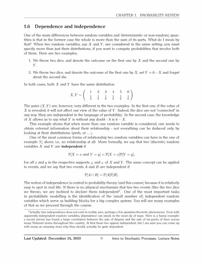
1.6 Dependence and independence
One of the main differences between random variables and (deterministic or non-random) quan-tities is that in the former case the whole is more than the sum of its parts. What do I mean bythat? When two random variables, say X and Y , are considered in the same setting, you mustspecify more than just their distributions, if you want to compute probabilities that involve bothof them. Here are two examples.
1. We throw two dice, and denote the outcome on the first one by X and the second one byY .
2. We throw two dice, and denote the outcome of the first one by X , set Y = 6−X and forgetabout the second die.
In both cases, both X and Y have the same distribution
X,Y ∼
(1 2 3 4 5 616
16
16
16
16
16
)
The pairs (X,Y ) are, however, very different in the two examples. In the first one, if the value ofX is revealed, it will not affect our view of the value of Y . Indeed, the dice are not “connected” inany way (they are independent in the language of probability). In the second case, the knowledgeof X allows us to say what Y is without any doubt - it is 6−X .
This example shows that when more than one random variable is considered, one needs toobtain external information about their relationship - not everything can be deduced only bylooking at their distributions (pmfs, or . . . ).
One of the most common forms of relationship two random variables can have is the one ofexample (1) above, i.e., no relationship at all. More formally, we say that two (discrete) randomvariables X and Y are independent if
P[X = x and Y = y] = P[X = x]P[Y = y],
for all x and y in the respective supports X and Y of X and Y . The same concept can be appliedto events, and we say that two events A and B are independent if
P[A ∩B] = P[A]P[B].
The notion of independence is central to probability theory (and this course) because it is relativelyeasy to spot in real life. If there is no physical mechanism that ties two events (like the two dicewe throw), we are inclined to declare them independent2. One of the most important tasksin probabilistic modelling is the identification of the (small number of) independent randomvariables which serve as building blocks for a big complex system. You will see many examplesof that as we proceed through the course.
2Actually, true independence does not exist in reality, save, perhaps a few quantum-theoretic phenomena. Even withapparently independent random variables, dependence can sneak in the most sly of ways. Here is a funny example:a recent survey has found a large correlation between the sale of diapers and the sale of six-packs of beer acrossmany Walmart stores throughout the country. At first these two appear independent, but I am sure you can come upwith many an amusing story why they should, actually, be quite dependent.
Last Updated: December 24, 2010 9 Intro to Stochastic Processes: Lecture Notes
CHAPTER 1. PROBABILITY REVIEW
1.7 Conditional probability
When two random variables are not independent, we still want to know how the knowledge ofthe exact value of one of the affects our guesses about the value of the other. That is what theconditional probability is for. We start with the definition, and we state it for events first: for twoevents A, B such that P[B] > 0, the conditional probability P[A|B] of A given B is defined as:
P[A|B] =P[A ∩B]
P[B].
The conditional probability is not defined when P[B] = 0 (otherwise, we would be computing00 - why?). Every statement in the sequel which involves conditional probability will be assumedto hold only when P[B] = 0, without explicit mention.
The conditional probability calculations often use one of the following two formulas. Bothof them use the familiar concept of partition. If you forgot what it is, here is a definition: acollection A1, A2, . . . , An of events is called a partition of Ω if a) A1 ∪ A2 ∪ . . . An = Ω and b)Ai ∩ Aj = ∅ for all pairs i, j = 1, . . . , n with i 6= j . So, let A1, . . . , An be a partition of Ω, and letB be an event.
1. The Law of Total Probability.
P[B] =n∑i=1
P[B|Ai]P[Ai].
2. Bayes formula. For k = 1, . . . , n, we have
P[Ak|B] =P[B|Ak]P[Ak]∑ni=1 P[B|Ai]P[Ai]
.
Even though the formulas above are stated for finite partitions, they remain true when the numberof Ak ’s is countably infinite. The finite sums have to be replaced by infinite series, however.
Random variables can be substituted for events in the definition of conditional probability asfollows: for two random variables X and Y , the conditional probabilty that X = x, given Y = y(with x and y in respective supports X and Y ) is given by
P[X = x|Y = y] =P[X = x and Y = y]
P[Y = y].
The formula above produces a different probability distribution for each y. This is called theconditional distribution of X , given Y = y. We give a simple example to illustrate this concept.Let X be the number of heads obtained when two coins are thrown, and let Y be the indicatorof the event that the second coin shows heads. The distribution of X is Binomial:
X ∼
(0 1 214
12
14
),
or, in the more compact notation which we use when the support is clear from the contextX ∼ (14 ,
12 ,
14). The random variable Y has the Bernoulli distribution Y = (12 ,
12). What happens
Last Updated: December 24, 2010 10 Intro to Stochastic Processes: Lecture Notes

CHAPTER 1. PROBABILITY REVIEW
to the distribution of X , when we are told that Y = 0, i.e., that the second coin shows heads. Inthat case we have
P[X = x|Y = 0] =
P[X=0,Y=0]
P[Y=0] = P[ the pattern is TT ]P[Y=0] = 1/4
1/2 = 12 , x = 0
P[X=1,Y=0]P[Y=0] = P[ the pattern is HT ]
P[Y=0] = 1/41/2 = 1
2 , x = 1P[X=2,Y=0]
P[Y=0] = P[ well, there is no such pattern ]P[Y=0] = 0
1/2 = 0 , x = 2
Thus, the conditional distribution of X , given Y = 0, is (12 ,12 , 0). A similar calculation can be used
to get the conditional distribution of X , but now given that Y = 1, is (0, 12 ,12). The moral of the
story is that the additional information contained in Y can alter our views about the unknownvalue of X using the concept of conditional probability. One final remark about the relationshipbetween independence and conditional probability: suppose that the random variables X and Yare independent. Then the knowledge of Y should not affect how we think about X ; indeed, then
P[X = x|Y = y] =P[X = x, Y = y]
P[Y = y]=
P[X = x]P[Y = y]
P[Y = y]= P[X = x].
The conditional distribution does not depend on y, and coincides with the unconditional one.The notion of independence for two random variables can easily be generalized to larger
collections
Definition 1.6. Random variables X1, X2, . . . , Xn are said to be independent if
P[X1 = x1, X2 = x2, . . . Xn = xn] = P[X1 = x1]P[X2 = x2] . . .P[Xn = xn]
for all x1, x2, . . . , xn.An infinite collection of random variables is said to be independent if all of its finite subcol-
lections are independent.
Independence is often used in the following way:
Proposition 1.7. Let X1, . . . , Xn be independent random variables. Then
1. g1(X1), . . . , gn(Xn) are also independent for (practically) all functions g1, . . . , gn,
2. if X1, . . . , Xn are integrable then the product X1 . . . Xn is integrable and
E[X1 . . . Xn] = E[X1] . . .E[Xn], and
3. if X1, . . . , Xn are square-integrable, then
Var[X1 + · · ·+Xn] = Var[X1] + · · ·+ Var[Xn].
EquivalentlyCov[Xi, Xj ] = E[(X1 − E[X1])(X2 − E[X2])] = 0,
for all i 6= j ∈ 1, 2, . . . , n.
Remark 1.8. The last statement says that independent random variables are uncorrelated. Theconverse is not true. There are uncorrelated random variables which are not independent.
Last Updated: December 24, 2010 11 Intro to Stochastic Processes: Lecture Notes
CHAPTER 1. PROBABILITY REVIEW
When several random variables (X1, X2, . . . Xn) are considered in the same setting, we of-ten group them together into a random vector. The distribution of the random vector X =(X1, . . . , Xn) is the collection of all probabilities of the form
P[X1 = x1, X2 = x2, . . . , Xn = xn],
when x1, x2, . . . , xn range through all numbers in the appropriate supports. Unlike in the caseof a single random variable, writing down the distributions of random vectors in tables is a bitmore difficult. In the two-dimensional case, one would need an entire matrix, and in the higherdimensions some sort of a hologram would be the only hope.
The distributions of the components X1, . . . , Xn of the random vector X are called themarginal distributions of the random variables X1, . . . , Xn. When we want to stress the fact thatthe random variables X1, . . . , Xn are a part of the same random vector, we call the distributionof X the joint distribution of X1, . . . , Xn. It is important to note that, unless random variablesX1, . . . , Xn are a priori known to be independent, the joint distribution holds more informationabout X than all marginal distributions together.
1.8 Examples
Here is a short list of some of the most important discrete random variables. You will learn aboutgenerating functions soon.
Example 1.9.
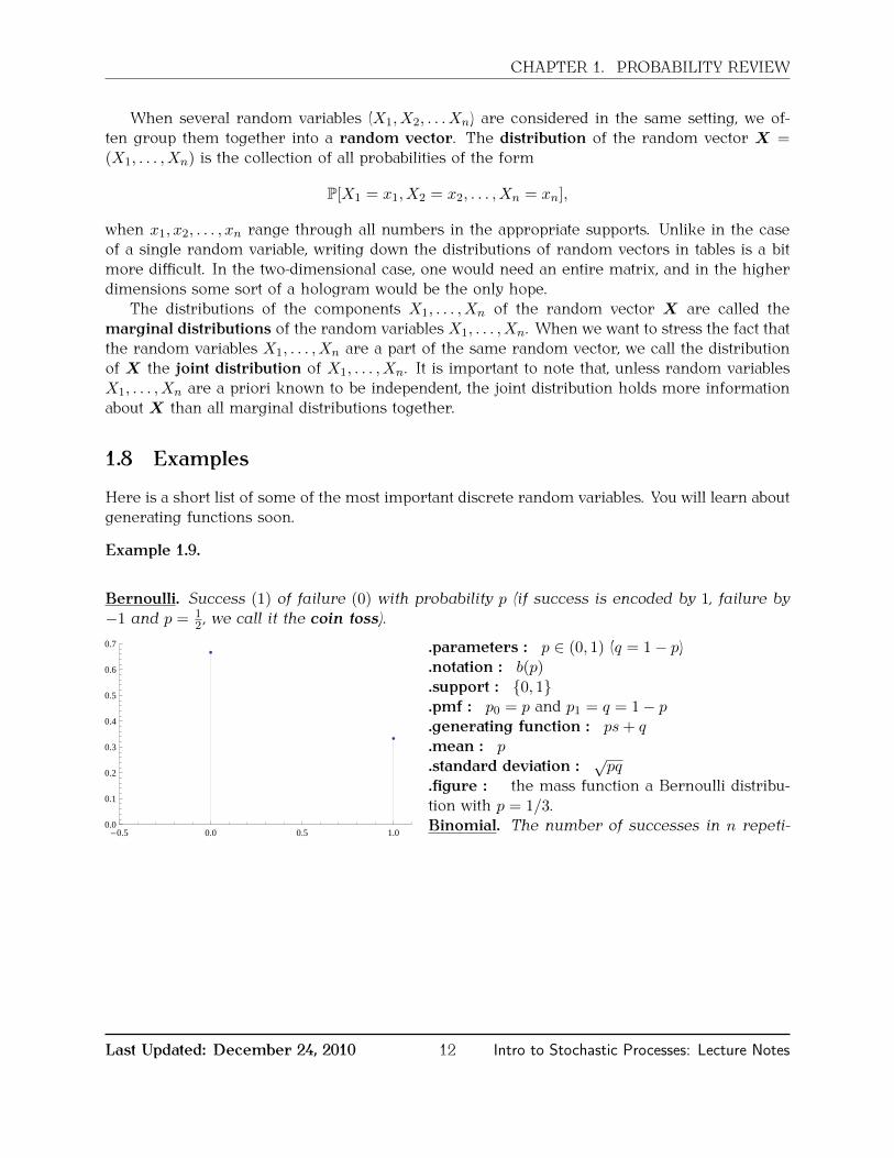
Bernoulli. Success (1) of failure (0) with probability p (if success is encoded by 1, failure by−1 and p = 1
2 , we call it the coin toss).
-0.5 0.0 0.5 1.00.0
0.1
0.2
0.3
0.4
0.5
0.6
0.7 .parameters : p ∈ (0, 1) (q = 1− p).notation : b(p).support : 0, 1.pmf : p0 = p and p1 = q = 1− p.generating function : ps+ q.mean : p.standard deviation : √pq.figure : the mass function a Bernoulli distribu-tion with p = 1/3.Binomial. The number of successes in n repeti-
Last Updated: December 24, 2010 12 Intro to Stochastic Processes: Lecture Notes

CHAPTER 1. PROBABILITY REVIEW
tions of a Bernoulli trial with success probabilityp.
0 10 20 30 40 50
0.05
0.10
0.15
0.20
0.25
0.30 .parameters : n ∈ N, p ∈ (0, 1) (q = 1− p).notation : b(n, p).support : 0, 1, . . . , n.pmf : pk =
(nk
)pkqn−k , k = 0, . . . , n
.generating function : (ps+ q)n
.mean : np
.standard deviation : √npq
.figure : mass functions of three binomial dis-tributions with n = 50 and p = 0.05 (blue), p = 0.5(purple) and p = 0.8 (yellow).
Poisson. The number of spelling mistakes one makes while typing a single page.
0 5 10 15 20 25
0.1
0.2
0.3
0.4.parameters : λ > 0.notation : p(n, p).support : N0
.pmf : pk = e−λ λk
k! , k ∈ N0
.generating function : eλ(s−1)
.mean : λ
.standard deviation :√λ
.figure : mass functions of two Poisson distribu-tions with parameters λ = 0.9 (blue) and λ = 10(purple).
Geometric. The number of repetitions of a Bernoulli trial with parameter p until the firstsuccess.
0 5 10 15 20 25 30
0.05
0.10
0.15
0.20
0.25
0.30 .parameters : p ∈ (0, 1), q = 1− p.notation : g(p).support : N0
.pmf : pk = pqk−1, k ∈ N0
.generating function : p1−qs
.mean : qp
.standard deviation :√qp
.figure : mass functions of two Geometric distri-butions with parameters p = 0.1 (blue) and p = 0.4(purple).
Last Updated: December 24, 2010 13 Intro to Stochastic Processes: Lecture Notes

CHAPTER 1. PROBABILITY REVIEW
Negative Binomial. The number of failures it takes to obtain r successes in repeated indepen-dent Bernoulli trials with success probability p.
0 20 40 60 80 100
0.05
0.10
0.15
0.20
0.25
0.30 .parameters : r ∈ N, p ∈ (0, 1) (q = 1− p).notation : g(n, p).support : N0
.pmf : pk =(−rk
)prqk , k =∈ N0
.generating function :(
p1−qs
)r.mean : r qp
.standard deviation :√qrp
.figure : mass functions of two negative bino-mial distributions with r = 100, p = 0.6 (blue) andr = 25, p = 0.9 (purple).
Last Updated: December 24, 2010 14 Intro to Stochastic Processes: Lecture Notes
Chapter 2
Mathematica in 15 min
Mathematica is a glorified calculator. Here is how to use it1.
2.1 Basic Syntax
• Symbols +, -, /, ^, * are all supported by Mathematica. Multiplication can be repre-sented by a space between variables. a x + b and a*x + b are identical.
• Warning: Mathematica is case-sensitive. For example, the command to exit is Quit andnot quit or QUIT.
• Brackets are used around function arguments. Write Sin[x], not Sin(x) or Sinx.
• Parentheses ( ) group terms for math operations: (Sin[x]+Cos[y])*(Tan[z]+z^2).
• If you end an expression with a ; (semi-colon) it will be executed, but its output will not beshown. This is useful for simulations, e.g.
• Braces are used for lists:
In[1]:= A = 81, 2, 3<
Out[1]= 81, 2, 3<
• Names can refer to variables, expressions, functions, matrices, graphs, etc. A name isassigned using name = object. An expression may contain undefined names:
In[5]:= A = Ha + bL^3
Out[5]= Ha + bL3
In[6]:= A^2
Out[6]= Ha + bL6
1Actually, this is just a tip of the iceberg. It can do many many many other things.
15

CHAPTER 2. MATHEMATICA IN 15 MIN
• The percent sign % stores the value of the previous result
In[7]:= 5 + 3
Out[7]= 8
In[8]:= %^2
Out[8]= 64
2.2 Numerical Approximation
• N[expr] gives the approximate numerical value of expression, variable, or command:
In[9]:= N@Sqrt@2DD
Out[9]= 1.41421
• N[%] gives the numerical value of the previous result:
In[17]:= E + Pi
Out[17]= ã + Π
In[18]:= N@%D
Out[18]= 5.85987
• N[expr,n] gives n digits of precision for the expression expr:
In[14]:= N@Pi, 30D
Out[14]= 3.14159265358979323846264338328
• Expressions whose result can’t be represented exactly don’t give a value unless you requestapproximation:
In[11]:= Sin@3D
Out[11]= Sin@3D
In[12]:= N@Sin@3DD
Out[12]= 0.14112
2.3 Expression Manipulation
• Expand[expr] (algebraically) expands the expression expr:
Last Updated: December 24, 2010 16 Intro to Stochastic Processes: Lecture Notes

CHAPTER 2. MATHEMATICA IN 15 MIN
In[19]:= Expand@Ha + bL^2D
Out[19]= a2 + 2 a b + b2
• Factor[expr] factors the expression expr
In[20]:= Factor@ a^2 - b^2D
Out[20]= Ha - bL Ha + bL
In[21]:= Factor@ x^2 - 5 x + 6D
Out[21]= H-3 + xL H-2 + xL
• Simplify[expr] performs all kinds of simplifications on the expression expr:
In[35]:= A = xHx - 1L - xH1 + xL
Out[35]= x
-1 + x-
x
1 + x
In[36]:= Simplify@AD
Out[36]= 2 x
-1 + x2
2.4 Lists and Functions
• If L is a list, its length is given by Length[L]. The nth element of L can be accessed byL[[n]] (note the double brackets):
In[43]:= L = 82, 4, 6, 8, 10<
Out[43]= 82, 4, 6, 8, 10<
In[44]:= L@@3DD
Out[44]= 6
• Addition, subtraction, multiplication and division can be applied to lists element by element:
In[1]:= L = 81, 3, 4<; K = 83, 4, 2<;
In[2]:= L + K
Out[2]= 84, 7, 6<
In[3]:= LK
Out[3]= : 1
3, 3
4, 2>
Last Updated: December 24, 2010 17 Intro to Stochastic Processes: Lecture Notes

CHAPTER 2. MATHEMATICA IN 15 MIN
• If the expression expr depends on a variable (say i), Table[expr,i,m,n] produces a listof the values of the expression expr as i ranges from m to n
In[37]:= Table@i^2, 8i, 0, 5<D
Out[37]= 80, 1, 4, 9, 16, 25<
• The same works with two indices - you will get a list of lists
In[40]:= Table@i^j, 8i, 1, 3<, 8j, 2, 3<D
Out[40]= 881, 1<, 84, 8<, 89, 27<<
• It is possible to define your own functions in Mathematica. Just use the underscore syntaxf[x_]=expr, where expr is some expression involving x:
In[47]:= f@x_D = x^2
Out[47]= x2
In[48]:= f@x + yD
Out[48]= Hx + yL2
• To apply the function f (either built-in, like Sin, or defined by you) to each element of thelist L, you can use the command Map with syntax Map[f,L]:
In[50]:= f@x_D = 3*x
Out[50]= 3 x
In[51]:= L = 81, 2, 3, 4<
Out[51]= 81, 2, 3, 4<
In[52]:= Map@f, LD
Out[52]= 83, 6, 9, 12<
• If you want to add all the elements of a list L, use Total[L]. The list of the same lengthas L, but whose kth element is given by the sum of the first k elements of L is given byAccumulate[L]:
In[8]:= L = 81, 2, 3, 4, 5<
Out[8]= 81, 2, 3, 4, 5<
In[9]:= Accumulate@LD
Out[9]= 81, 3, 6, 10, 15<
In[10]:= Total@LD
Out[10]= 15
Last Updated: December 24, 2010 18 Intro to Stochastic Processes: Lecture Notes

CHAPTER 2. MATHEMATICA IN 15 MIN
2.5 Linear Algebra
• In Mathematica, matrix is a nested list, i.e., a list whose elements are lists. By convention,matrices are represented row by row (inner lists are row vectors).
• To access the element in the ith row and jth column of the matrix A, type A[[i,j]] orA[[i]][[j]]:
In[59]:= A = 882, 1, 3<, 85, 6, 9<<
Out[59]= 882, 1, 3<, 85, 6, 9<<
In[60]:= A@@2, 3DD
Out[60]= 9
In[61]:= A@@2DD@@3DD
Out[61]= 9
• Matrixform[expr] displays expr as a matrix (provided it is a nested list)
In[9]:= A = Table@i*2^j, 8i, 2, 5<, 8j, 1, 2<D
Out[9]= 884, 8<, 86, 12<, 88, 16<, 810, 20<<
In[10]:= MatrixForm@AD
Out[10]//MatrixForm=
i
k
jjjjjjjjjjjjjj
4 8
6 12
8 16
10 20
y
zzzzzzzzzzzzzz
• Commands Transpose[A], Inverse[A], Det[A], Tr[A] and MatrixRank[A] return the trans-pose, inverse, determinant, trace and rank of the matrix A, respectively.
• To compute the nth power of the matrix A, use MatrixPower[A,n]
In[21]:= A = 881, 1<, 81, 0<<
Out[21]= 881, 1<, 81, 0<<
In[22]:= MatrixForm@MatrixPower@A, 5DD
Out[22]//MatrixForm=
i
kjjj8 5
5 3y
zzz
• Identity matrix of order n is produced by IdentityMatrix[n].
• If A and B are matrices of the same order, A+B and A-B are their sum and difference.
Last Updated: December 24, 2010 19 Intro to Stochastic Processes: Lecture Notes

CHAPTER 2. MATHEMATICA IN 15 MIN
• If A and B are of compatible orders, A.B (that is a dot between them) is the matrix productof A and B.
• For a square matrix A, CharacteristicPolynomial[A,x] is the characteristic poynomial,det(xI −A) in the variable x:
In[40]:= A = 883, 4<, 82, 1<<
Out[40]= 883, 4<, 82, 1<<
In[42]:= CharacteristicPolynomial@A, xD
Out[42]= -5 - 4 x + x2
• To get eigenvalues and eigenvectors use Eigenvalues[A] and Eigenvectors[A]. The re-sults will be the list containing the eigenvalues in the Eigenvalues case, and the list ofeigenvectors of A in the Eigenvectors case:
In[52]:= A = 883, 4<, 82, 1<<
Out[52]= 883, 4<, 82, 1<<
In[53]:= Eigenvalues@AD
Out[53]= 85, -1<
In[54]:= Eigenvectors@AD
Out[54]= 882, 1<, 8-1, 1<<
2.6 Predefined Constants
• A number of constants are predefined by Mathematica: Pi, I (√−1), E (2.71828...), Infinity.
Don’t use I, E (or D) for variable names - Mathematica will object.
• A number of standard functions are built into Mathematica: Sqrt[], Exp[], Log[], Sin[],ArcSin[], Cos[], etc.
2.7 Calculus
• D[f,x] gives the derivative of f with respect to x. For the first few derivatives you can usef’[x], f’’[x], etc.
In[66]:= D@ x^k, xD
Out[66]= k x-1+k
• D[f,x,n] gives the nth derivative of f with respect to x
• D[f,x,y] gives the mixed derivative of f with respect to x and y.
Last Updated: December 24, 2010 20 Intro to Stochastic Processes: Lecture Notes

CHAPTER 2. MATHEMATICA IN 15 MIN
• Integrate[f,x] gives the indefinite integral of f with respect to x:
In[67]:= Integrate@Log@xD, xD
Out[67]= -x + x Log@xD
• Integrate[f,x,a,b] gives the definite integral of f on the interval [a, b] (a or b can beInfinity (∞) or -Infinity (−∞)) :
In[72]:= Integrate@Exp@-2*xD, 8x, 0, Infinity<D
Out[72]= 1
2
• NIntegrate[f,x,a,b] gives the numerical approximation of the definite integral. Thisusually returns an answer when Integrate[] doesn’t work:
In[76]:= Integrate@1Hx + Sin@xDL, 8x, 1, 2<D
Out[76]= à1
2
1
x + Sin@xD âx
In[77]:= NIntegrate@1Hx + Sin@xDL, 8x, 1, 2<D
Out[77]= 0.414085
• Sum[expr,n,a,b] evaluates the (finite or infinite) sum. Use NSum for a numerical approx-imation.
In[80]:= Sum@1k^4, 8k, 1, Infinity<D
Out[80]= Π4
90
• DSolve[eqn,y,x] solves (given the general solution to) an ordinary differential equation forfunction y in the variable x:
In[88]:= DSolve@y’’@xD + y@xD x, y@xD, xD
Out[88]= 88y@xD ® x + C@1D Cos@xD + C@2D Sin@xD<<
• To calculate using initial or boundary conditions use DSolve[eqn,conds,y,x]:
In[93]:= DSolve@8y’@xD y@xD^2, y@0D 1<, y@xD, xD
Out[93]= ::y@xD ® 1
1 - x>>
Last Updated: December 24, 2010 21 Intro to Stochastic Processes: Lecture Notes

CHAPTER 2. MATHEMATICA IN 15 MIN
2.8 Solving Equations
• Algebraic equations are solved with Solve[lhs==rhs,x], where x is the variable with re-spect to which you want to solve the equation. Be sure to use == and not = in equations.Mathematica returns the list with all solutions:
In[81]:= Solve@ x^3 x, xD
Out[81]= 88x ® -1<, 8x ® 0<, 8x ® 1<<
• FindRoot[f,x,x0] is used to find a root when Solve[] does not work. It solves for xnumerically, using an initial value of x0:
In[82]:= FindRoot@Cos@xD x, 8x, 1<D
Out[82]= 8x ® 0.739085<
2.9 Graphics
• Plot[expr,x,a,b] plots the expression expr, in the variable x, from a to b:
In[83]:= Plot@Sin@xD, 8x, 1, 3<D
Out[83]=
1.5 2.0 2.5 3.0
0.4
0.6
0.8
1.0
• Plot3D[expr,x,a,b,y,c,d] produces a 3D plot in 2 variables:
In[84]:= Plot3D@Sin@x^2 + y^2D, 8x, 2, 3<, 8y, -2, 4<D
Out[84]=
2.0
2.5
3.0-2
0
2
4
-1.0
-0.5
0.0
0.5
1.0
Last Updated: December 24, 2010 22 Intro to Stochastic Processes: Lecture Notes

CHAPTER 2. MATHEMATICA IN 15 MIN
• If L is a list of the form L= x1, y1, x2, y2, . . . , xn, yn, you can use the commandListPlot[L] to display a graph consisting of points (x1, y1), . . . , (xn, yn):
In[11]:= L = Table@8i, i^2<, 8i, 0, 4<D
Out[11]= 880, 0<, 81, 1<, 82, 4<, 83, 9<, 84, 16<<
In[12]:= ListPlot@LD
Out[12]=
1 2 3 4
5
10
15
2.10 Probability Distributions and Simulation
• PDF[distr,x] and CDF[distr,x] return the pdf (pmf in the discrete case) and the cdf ofthe distribution distr in the variable x. distr can be one of:
– NormalDistribution[m,s],– ExponentialDistribution[l],– UniformDistribution[a,b],– BinomialDistribusion[n,p],
and many many others (see ?PDF and follow various links from there).
• Use ExpectedValue[expr,distr,x] to compute the expectation E[f(X)], where expr is theexpression for the function f in the variable x:
In[23]:= distr = PoissonDistribution@ΛD
Out[23]= PoissonDistribution@ΛD
In[25]:= PDF@distr, xD
Out[25]= ã-ΛΛx
x!
In[27]:= ExpectedValue@x^3, distr, xD
Out[27]= Λ + 3 Λ2 + Λ3
• There is no command for the generating function, but you can get it by computing the char-acteristic function and changing the variable a bit CharacteristicFunction[distr, - I Log[s]]:
Last Updated: December 24, 2010 23 Intro to Stochastic Processes: Lecture Notes

CHAPTER 2. MATHEMATICA IN 15 MIN
In[22]:= distr = PoissonDistribution@ΛD
Out[22]= PoissonDistribution@ΛD
In[23]:= CharacteristicFunction@distr, -I Log@sDD
Out[23]= ãH-1+sL Λ
• To get a random number (unifomly distributed between 0 and 1) use RandomReal[]. A uni-formly distributed random number on the interval [a, b] can be obtained by RandomReal[a,b].For a list of n uniform random numbers on [a, b] write RandomReal[a,b,n].
In[2]:= RandomReal@D
Out[2]= 0.168904
In[3]:= RandomReal@87, 9<D
Out[3]= 7.83027
In[5]:= RandomReal@80, 1<, 3D
Out[5]= 80.368422, 0.961658, 0.692345<
• If you need a random number from a particular continuous distribution (normal, say), useRandomReal[distr] or RandomReal[distr,n] if you need n draws.
• When drawing from a discrete distribution use RandomInteger instead.
• If L is a list of numbers, Histogram[L] displays a histogram of L (you need to load thepackage Histograms by issuing the command <<Histograms‘ before you can use it):
In[7]:= L = RandomReal@NormalDistribution@0, 1D, 100D;
In[10]:= << Histograms‘
In[12]:= Histogram@LD
Out[12]=
-2 -1 0 1 2
5
10
15
20
2.11 Help Commands
• ?name returns information about name
• ??name adds extra information about name
• Options[command] returns all options that may be set for a given command
Last Updated: December 24, 2010 24 Intro to Stochastic Processes: Lecture Notes

CHAPTER 2. MATHEMATICA IN 15 MIN
• ?pattern returns the list of matching names (used when you forget a command). patterncontains one or more asterisks * which match any string. Try ?*Plot*
2.12 Common Mistakes
• Mathematica is case sensitive: Sin is not sin
• Don’t confuse braces, brackets, and parentheses , [], ()
• Leave spaces between variables: write a x^2 instead of ax^2, if you want to get ax2.
• Matrix multiplication uses . instead of * or a space.
• Don’t use = instead of == in Solve or DSolve
• If you are using an older version of Mathematica, a function might be defined in an externalmodule which has to be loaded before the function can be used. For example, in someversions, the command <<Graphics’ needs to be given before any plots can be made. Thesymbol at the end is not an apostrophe - it is the dash above the TAB key.
• Using Integrate[] around a singular point can yield wrong answers. (Use NIntegrate[]to check.)
• Don’t forget the underscore _ when you define a function.
Last Updated: December 24, 2010 25 Intro to Stochastic Processes: Lecture Notes

Chapter 3
Stochastic Processes
Definition 3.1. Let T be a subset of [0,∞). A family of random variables Xtt∈T , indexed byT , is called a stochastic (or random) process. When T = N (or T = N0), Xtt∈T is said to bea discrete-time process, and when T = [0,∞), it is called a continuous-time process.
When T is a singleton (say T = 1), the process Xtt∈T ≡ X1 is really just a single randomvariable. When T is finite (e.g., T = 1, 2, . . . , n), we get a random vector. Therefore, stochasticprocesses are generalizations of random vectors. The interpretation is, however, somewhatdifferent. While the components of a random vector usually (not always) stand for different spatialcoordinates, the index t ∈ T is more often than not interpreted as time. Stochastic processesusually model the evolution of a random system in time. When T = [0,∞) (continuous-timeprocesses), the value of the process can change every instant. When T = N (discrete-timeprocesses), the changes occur discretely.
In contrast to the case of random vectors or random variables, it is not easy to define a notionof a density (or a probability mass function) for a stochastic process. Without going into detailswhy exactly this is a problem, let me just mention that the main culprit is the infinity. One usuallyconsiders a family of (discrete, continuous, etc.) finite-dimensional distributions, i.e., the jointdistributions of random vectors
(Xt1 , Xt2 , . . . , Xtn),
for all n ∈ N and all choices t1, . . . , tn ∈ T .The notion of a stochastic processes is very important both in mathematical theory and its
applications in science, engineering, economics, etc. It is used to model a large number of variousphenomena where the quantity of interest varies discretely or continuously through time in anon-predictable fashion.
Every stochastic process can be viewed as a function of two variables - t and ω. For eachfixed t, ω 7→ Xt(ω) is a random variable, as postulated in the definition. However, if we changeour point of view and keep ω fixed, we see that the stochastic process is a function mapping ω tothe real-valued function t 7→ Xt(ω). These functions are called the trajectories of the stochasticprocess X .
26
CHAPTER 3. STOCHASTIC PROCESSES
æ
æ
æ
æ
æ
æ
æ
æ
æ
æ
æ
æ
æ
æ
æ
æ
æ
æ
æ
æ
æ
5 10 15 20
-6
-4
-2
2
4
6
æ
æ
æ
æ
æ
æ
æ
æ
æ
æ
æ
æ
æ
æ
æ
æ
æ
æ
æ
æ
æ
5 10 15 20
-6
-4
-2
2
4
6
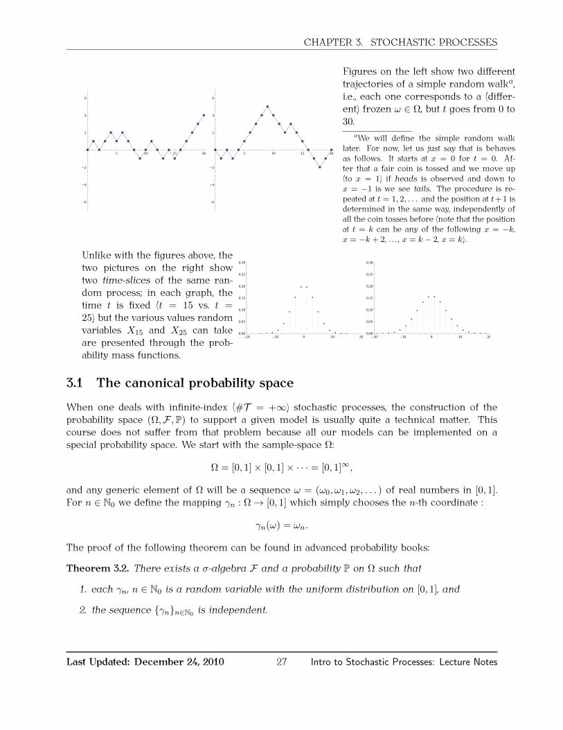
Figures on the left show two differenttrajectories of a simple random walka,i.e., each one corresponds to a (differ-ent) frozen ω ∈ Ω, but t goes from 0 to30.
aWe will define the simple random walklater. For now, let us just say that is behavesas follows. It starts at x = 0 for t = 0. Af-ter that a fair coin is tossed and we move up(to x = 1) if heads is observed and down tox = −1 is we see tails. The procedure is re-peated at t = 1, 2, . . . and the position at t+1 isdetermined in the same way, independently ofall the coin tosses before (note that the positionat t = k can be any of the following x = −k,x = −k + 2, . . . , x = k − 2, x = k).
Unlike with the figures above, thetwo pictures on the right showtwo time-slices of the same ran-dom process; in each graph, thetime t is fixed (t = 15 vs. t =25) but the various values randomvariables X15 and X25 can takeare presented through the prob-ability mass functions.
-20 -10 0 10 200.00
0.05
0.10
0.15
0.20
0.25
0.30
-20 -10 0 10 200.00
0.05
0.10
0.15
0.20
0.25
0.30
3.1 The canonical probability space
When one deals with infinite-index (#T = +∞) stochastic processes, the construction of theprobability space (Ω,F ,P) to support a given model is usually quite a technical matter. Thiscourse does not suffer from that problem because all our models can be implemented on aspecial probability space. We start with the sample-space Ω:
Ω = [0, 1]× [0, 1]× · · · = [0, 1]∞,
and any generic element of Ω will be a sequence ω = (ω0, ω1, ω2, . . . ) of real numbers in [0, 1].For n ∈ N0 we define the mapping γn : Ω→ [0, 1] which simply chooses the n-th coordinate :
γn(ω) = ωn.
The proof of the following theorem can be found in advanced probability books:
Theorem 3.2. There exists a σ-algebra F and a probability P on Ω such that
1. each γn, n ∈ N0 is a random variable with the uniform distribution on [0, 1], and
2. the sequence γnn∈N0 is independent.
Last Updated: December 24, 2010 27 Intro to Stochastic Processes: Lecture Notes

CHAPTER 3. STOCHASTIC PROCESSES
Remark 3.3. One should think of the sample space Ω as a source of all the randomness inthe system: the elementary event ω ∈ Ω is chosen by a process beyond out control and theexact value of ω is assumed to be unknown. All the other parts of the system are possiblycomplicated, but deterministic, functions of ω (random variables). When a coin is tossed, only asingle drop of randomness is needed - the outcome of a coin-toss. When several coins are tossed,more randomness is involved and the sample space must be bigger. When a system involves aninfinite number of random variables (like a stochastic process with infinite T ), a large samplespace Ω is needed.
3.2 Constructing the Random Walk
Let us show how to construct the simple random walk on the canonical probability space (Ω,F ,P)from Theorem 3.2. First of all, we need a definition of the simple random walk:
Definition 3.4. A stochastic process Xnn∈N0 is called a simple random walk if
1. X0 = 0,
2. the increment Xn+1 −Xn is independent of (X0, X1, . . . , Xn) for each n ∈ N0, and
3. the increment Xn+1 −Xn has the coin-toss distribution, i.e.
P[Xn+1 −Xn = 1] = P[Xn+1 −Xn = −1] = 12 .
For the sequence γnn∈N, given by Theorem 3.2, define the following, new, sequence ξnn∈Nof random variables:
ξn =
1, γn ≥ 1
2
−1, otherwise.
Then, we set
X0 = 0, Xn =n∑k=1
ξk, n ∈ N.
Intuitively, we use each ξn to emulate a coin toss and then define the value of the process X attime n as the cumulative sum of the first n coin-tosses.
Proposition 3.5. The sequence Xnn∈N0 defined above is a simple random walk.
Proof. (1) is trivially true. To get (2), we first note that the ξnn∈N is an independent sequence(as it has been constructed by an application of a deterministic function to each element of anindependent sequence γnn∈N). Therefore, the increment Xn+1 −Xn = ξn+1 is independent ofall the previous coin-tosses ξ1, . . . , ξn. What we need to prove, though, is that it is independentof all the previous values of the process X . These, previous, values are nothing but linearcombinations of the coin-tosses ξ1, . . . , ξn, so they must also be independent of ξn+1. Finally, toget (3), we compute
P[Xn+1 −Xn = 1] = P[ξn+1 = 1] = P[γn+1 ≥ 12 ] = 1
2 .
A similar computation shows that P[Xn+1 −Xn = −1] = 12 .
Last Updated: December 24, 2010 28 Intro to Stochastic Processes: Lecture Notes
CHAPTER 3. STOCHASTIC PROCESSES
3.3 Simulation
Another way of thinking about sample spaces, and randomness in general, is through the notionof simulation. Simulation is what I did to produce the two trajectories of the random walk above;a computer tossed a fair coin for me 30 times and I followed the procedure described aboveto construct a trajectory of the random walk. If I asked the computer to repeat the process, Iwould get different 30 coin-tosses1. This procedure is the exact same one we imagine nature (orcasino equipment) follows whenever a non-deterministic situation is involved. The difference is,of course, that if we use the random walk to model out winnings in a fair gamble, it is muchcheaper and faster to use the computer than to go out and stake (and possibly loose) largeamounts of money. Another obvious advantage of the simulation approach is that it can berepeated; a simulation can be run many times and various statistics (mean, variance, etc.) can becomputed.
More technically, every simulation involves two separate inputs. The first one if the actualsequence of outcomes of coin-tosses. The other one is the structure of the model - I have toteach the computer to “go up” if heads shows and to “go down” if tails show, and to repeatthe same procedure several times. In more complicated situations this structure will be morecomplicated. What is remarkable is that the first ingredient, the coin-tosses, will stay almost assimple as in the random walk case, even in the most complicated models. In fact, all we need isa sequence of so-called random numbers. You will see through the many examples presentedin this course that if I can get my computer to produce an independent sequence of uniformlydistributed numbers between 0 and 1 (these are the random numbers) I can simulate trajectoriesof all important stochastic processes. Just to start you thinking, here is how to produce a coin-tossfrom a random number: declare heads if the random number drawn is between 0 and 0.5, anddeclare tails otherwise.
3.3.1 Random number generation
Before we get into intricacies of simulation of complicated stochastic processes, let us spendsome time on the (seemingly) simple procedure of the generation of a single random number.In other words, how do you teach a computer to give you a random number between 0 and 1?Theoretically, the answer is You can’t!. In practice, you can get quite close. The question of whatactually constitutes a random number is surprisingly deep and we will not even touch it in thiscourse.
Suppose we have written a computer program, a random number generator (RNG) - call itrand - which produces a random number between 0 and 1 every time we call it. So far, thereis nothing that prevents rand from always returning the same number 0.4, or from alternatingbetween 0.3 and 0.83. Such an implementation of rand will, however, hardly qualify for anRNG since the values it spits out come in a predictable order. We should, therefore, requireany candidate for a random number generator to produce a sequence of numbers which is asunpredictable as possible. This is, admittedly, a hard task for a computer having only deterministicfunctions in its arsenal, and that is why the random generator design is such a difficult field. Thestate of the affairs is that we speak of good or less good random number generators, based onsome statistical properties of the produced sequences of numbers.
1Actually, I would get the exact same 30 coin-tosses with probability 0.000000001
Last Updated: December 24, 2010 29 Intro to Stochastic Processes: Lecture Notes

CHAPTER 3. STOCHASTIC PROCESSES
One of the most important requirements is that our RNG produce uniformly distributednumbers in [0, 1] - namely - the sequence of numbers produced by rand will have to cover theinterval [0, 1] evenly, and, in the long run, the number of random numbers in each subinterval[a, b] of [0, 1] should be proportional to the length of the interval b−a. This requirement if hardlyenough, because the sequence
0, 0.1, 0.2, . . . , 0.8, 0.9, 1, 0.05, 0.15, 0.25, . . . , 0.85, 0.95, 0.025, 0.075, 0.125, 0.175, . . .
will do the trick while being perfectly predictable.To remedy the inadequacy of the RNGs satisfying only the requirement of uniform distribu-
tion, we might require rand to have the property that the pairs of produced numbers cover thesquare [0, 1] × [0, 1] uniformly. That means that, in the long run, the proportion of pairs fallingin a patch A of the square [0, 1] × [0, 1] will be proportional to its area. Of course, one couldcontinue with such requirements and ask for triples, quadruples, . . . of random numbers to beuniform in [0, 1]3, [0, 1]4 . . . . The highest dimension n such that the RNG produces uniformlydistributed numbers in [0, 1]n is called the order of the RNG. A widely-used RNG called theMersenne Twister, has the order of 623.
Another problem with RNGs is that the numbers produced will start to repeat after a while(this is a fact of life and finiteness of your computer’s memory). The number of calls it takes fora RNG to start repeating its output is called the period of a RNG. You might have wondered howis it that an RNG produces a different number each time it is called, since, after all, it is only afunction written in some programming language. Most often, RNGs use a hidden variable calledthe random seed which stores the last output of rand and is used as an (invisible) input to thefunction rand the next time it is called. If we use the same seed twice, the RNG will producethe same number, and so the period of the RNG is limited by the number of possible seeds.It is worth remarking that the actual random number generators usually produce a “random”integer between 0 and some large number RAND_MAX, and report the result normalized (divided)by RAND_MAX to get a number in [0, 1).
3.3.2 Simulation of Random Variables
Having found a random number generator good enough for our purposes (the one used byMathematica is just fine), we might want to use it to simulate random variables with distributionsdifferent from the uniform on [0, 1] (coin-tosses, normal, exponential, . . . ). This is almost alwaysachieved through transformations of the output of a RNG, and we will present several methodsfor dealing with this problem. A typical procedure (see the Box-Muller method below for anexception) works as follows: a real (deterministic) function f : [0, 1]→ R - called the transforma-tion function - is applied to rand. The result is a random variable whose distribution depends onthe choice of f . Note that the transformation function is by no means unique. In fact, γ ∼ U [0, 1],then f(γ) and f(γ), where f(x) = f(1− x), have the same distribution (why?).
What follows is a list of procedures commonly used to simulate popular random variables:
1. Discrete Random Variables Let X have a discrete distribution given by
X ∼(x1 x2 . . . xnp1 p2 . . . pn
).
Last Updated: December 24, 2010 30 Intro to Stochastic Processes: Lecture Notes

CHAPTER 3. STOCHASTIC PROCESSES
For discrete distributions taking an infinite number of values we can always truncate at avery large n and approximate it with a distribution similar to the one of X .We know that the probabilities p1, p2, . . . , pn add-up to 1, so we define the numbers 0 = q0 <q1 < · · · < qn = 1 by
q0 = 0, q1 = p1, q2 = p1 + p2, . . . qn = p1 + p2 + · · ·+ pn = 1.
To simulate our discrete random variable X , we call rand and then return x1 if 0 ≤ rand <q1, return x2 if q1 ≤ rand < q2, and so on. It is quite obvious that this procedure indeedsimulates a random variable X . The transformation function f is in this case given by
f(x) =
x1, 0 ≤ x < q1
x2, q1 ≤ x < q2
. . .
xn, qn−1 ≤ x ≤ 1
2. The Method of Inverse Functions The basic observation in this method is that , forany continuous random variable X with the distribution function FX , the random variableY = FX(X) is uniformly distributed on [0, 1]. By inverting the distribution function FX andapplying it to Y , we recover X . Therefore, if we wish to simulate a random variable withan invertible distribution function F , we first simulate a uniform random variable on [0, 1](using rand) and then apply the function F−1 to the result. In other words, use f = F−1 asthe transformation function. Of course, this method fails if we cannot write F−1 in closedform.
Example 3.6. (Exponential Distribution) Let us apply the method of inverse functionsto the simulation of an exponentially distributed random variable X with parameter λ.Remember that the density fX of X is given by
fX(x) = λ exp(−λx), x > 0, and so FX(x) = 1− exp(−λx), x > 0,
and so F−1X (y) = − 1λ log(1− y). Since, 1−rand has the same U[0, 1]-distribution as rand, we
conclude that f(x) = − 1λ log(x) works as a transformation function in this case, i.e., that
− log( rand )
λ
has the required Exp(λ)-distribution.
Example 3.7. (Cauchy Distribution) The Cauchy distribution is defined through its densityfunction
fX(x) =1
π
1
(1 + x2).
The distribution function FX can be determined explicitly in this example:
FX(x) =1
π
∫ x
−∞
1
(1 + x2)dx =
1
π
(π2
+ arctan(x)), and so F−1X (y) = tan
(π(y − 1
2
)),
yielding that f(x) = tan(π(x − 12)) is a transformation function for the Cauchy random
variable, i.e., tan(π(rand− 0.5)) will simulate a Cauchy random variable for you.
Last Updated: December 24, 2010 31 Intro to Stochastic Processes: Lecture Notes

CHAPTER 3. STOCHASTIC PROCESSES
3. The Box-Muller method This method is useful for simulating normal random variables,since for them the method of inverse function fails (there is no closed-form expression forthe distribution function of a standard normal). Note that this method does not fall underthat category of transformation function methods as described above. You will see, though,that it is very similar in spirit. It is based on a clever trick, but the complete proof is a bittechnical, so we omit it.
Proposition 3.8. Let γ1 and γ2 be independent U[0, 1]-distributed random variables. Thenthe random variables
X1 =√−2 log(γ1) cos(2πγ2), X2 =
√−2 log(γ1) sin(2πγ2)
are independent and standard normal (N(0,1)).
Therefore, in order to simulate a normal random variable with mean µ = 0 and varianceσ2 = 1, we produce call the function rand twice to produce two random numbers rand1and rand2. The numbers
X1 =√−2 log(rand1) cos(2π rand2), X2 =
√−2 log(rand1) sin(2π rand2)
will be two independent normals. Note that it is necessary to call the function rand twice,but we also get two normal random numbers out of it. It is not hard to write a procedurewhich will produce 2 normal random numbers in this way on every second call, returnone of them and store the other for the next call. In the spirit of the discussion above, thefunction f = (f1, f2) : (0, 1]× [0, 1]→ R2 given by
f1(x, y) =√−2 log(x) cos(2πy), f2(x, y) =
√−2 log(x) sin(2πy).
can be considered a transformation function in this case.
4. Method of the Central Limit Theorem The following algorithm is often used to simulatea normal random variable:
(a) Simulate 12 independent uniform random variables (rands) - γ1, γ2, . . . , γ12.(b) Set X = γ1 + γ2 + · · ·+ γ12 − 6.
The distribution of X is very close to the distribution of a unit normal, although not exactlyequal (e.g. P[X > 6] = 0, and P[Z > 6] 6= 0, for a true normal Z). The reason why Xapproximates the normal distribution well comes from the following theorem
Theorem 3.9. Let X1, X2, . . . be a sequence of independent random variables, all hav-ing the same (square-integrable) distribution. Set µ = E[X1] (= E[X2] = . . . ) and σ2 =Var[X1] (= Var[X2] = . . . ). The sequence of normalized random variables
(X1 +X2 + · · ·+Xn)− nµσ√n
,
converges to the normal random variable (in a mathematically precise sense).
Last Updated: December 24, 2010 32 Intro to Stochastic Processes: Lecture Notes

CHAPTER 3. STOCHASTIC PROCESSES
The choice of exactly 12 rands (as opposed to 11 or 35) comes from practice: it seems toachieve satisfactory performance with relatively low computational cost. Also, the standarddeviation of a U [0, 1] random variable is 1/
√12, so the denominator σ
√n conveniently
becomes 1 for n = 12. It might seem a bit wasteful to use 12 calls of rand in order toproduce one draw from the unit normal. If you try it out, you will see, however, thatit is of comparable speed to the Box-Muller method described above; while Box-Mulleruses computationally expensive cos, sin,
√ and log, this method uses only addition andsubtraction. The final verdict of the comparison of the two methods will depend on thearchitecture you are running the code on, and the quality of the implementation of thefunctions cos, sin . . . .
5. Other methods There is a number of other methods for transforming the output of randinto random numbers with prescribed density (rejection method, Poisson trick, . . . ). Youcan read about them in the free online copy of Numerical recipes in C at
http://www.library.cornell.edu/nr/bookcpdf.html
3.4 Monte Carlo Integration
Having described some of the procedures and methods used for simulation of various randomobjects (variables, vectors, processes), we turn to an application in probability and numericalmathematics. We start off by the following version of the Law of Large Numbers which constitutesthe theory behind most of the Monte Carlo applications
Theorem 3.10. (Law of Large Numbers) Let X1, X2, . . . be a sequence of identically distributedrandom variables, and let g : R → R be function such that µ = E[g(X1)] (= E[g(X2)] = . . . )exists. Then
g(X1) + g(X2) + · · ·+ g(Xn)
n→ µ =
∫ ∞−∞
g(x)fX1(x) dx, as n→∞.
The key idea of Monte Carlo integration is the following
Suppose that the quantity y we are interested in can be written as y =∫∞−∞ g(x)fX(x) dx
for some random variable X with density fX and come function g, and that x1, x2, . . .are random numbers distributed according to the distribution with density fX . Thenthe average
1
n(g(x1) + g(x2) + · · ·+ g(xn)),
will approximate y.
It can be shown that the accuracy of the approximation behaves like 1/√n, so that you have
to quadruple the number of simulations if you want to double the precision of you approximation.
Last Updated: December 24, 2010 33 Intro to Stochastic Processes: Lecture Notes

CHAPTER 3. STOCHASTIC PROCESSES
Example 3.11.
1. (numerical integration) Let g be a function on [0, 1]. To approximate the integral∫ 10 g(x) dx
we can take a sequence of n (U[0,1]) random numbers x1, x2, . . . ,∫ 1
0g(x) dx ≈ g(x1) + g(x2) + · · ·+ g(xn)
n,
because the density of X ∼ U [0, 1] is given by
fX(x) =
1, 0 ≤ x ≤ 1
0, otherwise.
2. (estimating probabilities) Let Y be a random variable with the density function fY . Ifwe are interested in the probability P[Y ∈ [a, b]] for some a < b, we simulate n drawsy1, y2, . . . , yn from the distribution FY and the required approximation is
P[Y ∈ [a, b]] ≈ number of yn’s falling in the interval [a, b]
n.
One of the nicest things about the Monte-Carlo method is that even if the density of therandom variable is not available, but you can simulate draws from it, you can still preformthe calculation above and get the desired approximation. Of course, everything works inthe same way for probabilities involving random vectors in any number of dimensions.
3. (approximating π)We can devise a simple procedure for approximating π ≈ 3.141592 by using the Monte-Carlo method. All we have to do is remember that π is the area of the unit disk. Therefore,π/4 equals to the portion of the area of the unit disk lying in the positive quadrant, and wecan write
π
4=
∫ 1
0
∫ 1
0g(x, y) dxdy,
where
g(x, y) =
1, x2 + y2 ≤ 1
0, otherwise.
So, simulate n pairs (xi, yi), i = 1 . . . n of uniformly distributed random numbers and counthow many of them fall in the upper quarter of the unit circle, i.e. how many satisfyx2i + y2i ≤ 1, and divide by n. Multiply your result by 4, and you should be close to π. Howclose? Well, that is another story . . . Experiment!
Last Updated: December 24, 2010 34 Intro to Stochastic Processes: Lecture Notes

Chapter 4
The Simple Random Walk
4.1 Construction
We have defined and constructed a random walk Xnn∈N0 in the previous lecture. Our nexttask is to study some of its mathematical properties. Let us give a definition of a slightly moregeneral creature.
Definition 4.1. A sequence Xnn∈N0 of random variables is called a simple random walk (withparameter p ∈ (0, 1)) if
1. X0 = 0,
2. Xn+1 −Xn is independent of (X0, X1, . . . , Xn) for all n ∈ N, and
3. the random variable Xn+1 −Xn has the following distribution(−1 1q p
)where, as usual, q = 1− p.
If p = 12 , the random walk is called symmetric.
The adjective simple comes from the fact that the size of each step is fixed (equal to 1) andit is only the direction that is random. One can study more general random walks where eachstep comes from an arbitrary prescribed probability distribution.
Proposition 4.2. Let Xnn∈N0 be a simple random walk with parameter p. The distribution ofthe random variable Xn is discrete with support −n,−n+ 2, . . . , n− 2, n, and probabilities
pl = P[Xn = l] =
(nl+n2
)p(n+l)/2q(n−l)/2, l = −n,−n+ 2, . . . , n− 2, n. (4.1)
Proof. Xn is composed of n independent steps ξk = Xk+1 −Xk , k = 1, . . . , n, each of which goeseither up or down. In order to reach level l in those n steps, the number u of up-steps and thenumber d of downsteps must satisfy u− d = l (and u+ d = n). Therefore, u = n+l
2 and d = n−l2 .
35

CHAPTER 4. THE SIMPLE RANDOM WALK
The number of ways we can choose these u up-steps from the total of n is( n
n+l2
), which, with
the fact the probability of any trajectory with exactly u up-steps is puqn−u, gives the probability(4.1) above. Equivalently, we could have noticed that the random variable n+Xn
2 has the binomialb(n, p)-distribution.
The proof of Proposition 4.2 uses the simple idea already hinted at inthe previous lecture: view the random walk as a random trajectoryin some space of trajectories, and, compute the required probabilityby simply counting the number of trajectories in the subset (event)you are interested in, and adding them all together, weighted bytheir probabilities. To prepare the ground for the future results, letC be the set of all possible trajectories:
C = (x0, x1, . . . , xn) : x0 = 0, xk+1 − xk = ±1, k ≤ n− 1.
You can think of the first n steps of a random walk simply as aprobability distribution on the state-space C .
The figure on the right shows the superposition of all trajectoriesin C for n = 4 and a particular one - (0, 1, 0, 1, 2) - in red.
æ
æ
æ
æ
æ
æ
æ
æ
æ
æ
æ
æ
æ
æ
æ
æ
æ
æ
æ
ææ
æ
æ
æ
æ
æ
æ
æ
æ
ææ
æ
æ
æ
ææ
æ
æ
æ
æ
æ
æ
æ
æ
æ
æ
æ
æ
æ
ææ
æ
æ
æ
ææ
æ
æ
æ
æ
æ
æ
æ
æ
ææ
æ
æ
æ
æ
æ
æ
æ
æ
æ
æ
æ
æ
æ
æ
æ
æ
æ
æ
æ
1 2 3 4
-4
-2
2
4
4.2 The maximum
Now we know how to compute the probabilties related to the position of the random walkXnn∈N0 at a fixed future time n. A mathematically more interesting question can be posedabout the maximum of the random walk on 0, 1, . . . , n. A nice expression for this probabilityis available for the case of symmetric simple random walks.
Proposition 4.3. Let Xnn∈N0 be a symmetric simple random walk, suppose n ≥ 2, and letMn = max(X0, . . . , Xn) be the maximal value of Xnn∈N0 on the interval 0, 1, . . . , n. Thesupport of Mn is 0, 1, . . . , n and its probability mass function is given by
pl = P[Mn = l] =
(n
bn+l+12 c
)2−n, l = 0, . . . , n.
Proof. Let us first pick a level l ∈ 0, 1, . . . , n and compute the auxilliary probability ql = P[Mn ≥l] by counting the number of trajectories whose maximal level reached is at least l. Indeed,the symmetry assumption ensures that all trajectories are equally likely. More precisely, letAl ⊂ C0(n) be given by
Al = (x0, x1, . . . , xn) ∈ C : maxk=0,...,n
xk ≥ l
= (x0, x1, . . . , xn) ∈ C : xk ≥ l, for at least one k ∈ 0, . . . , n.
Then P[Mn ≥ l] = 12n #Al , where #A denotes the number of elements in the set A. When l = 0,
we clearly have P[Mn ≥ 0] = 1, since X0 = 0.To count the number of elements in Al , we use the following clever observation (known as
the reflection principle):
Last Updated: December 24, 2010 36 Intro to Stochastic Processes: Lecture Notes
CHAPTER 4. THE SIMPLE RANDOM WALK
Claim 4.4. For l ∈ N, we have
#Al = 2#(x0, x1, . . . , xn) : xn > l+ #(x0, x1, . . . , xn) : xn = l. (4.2)
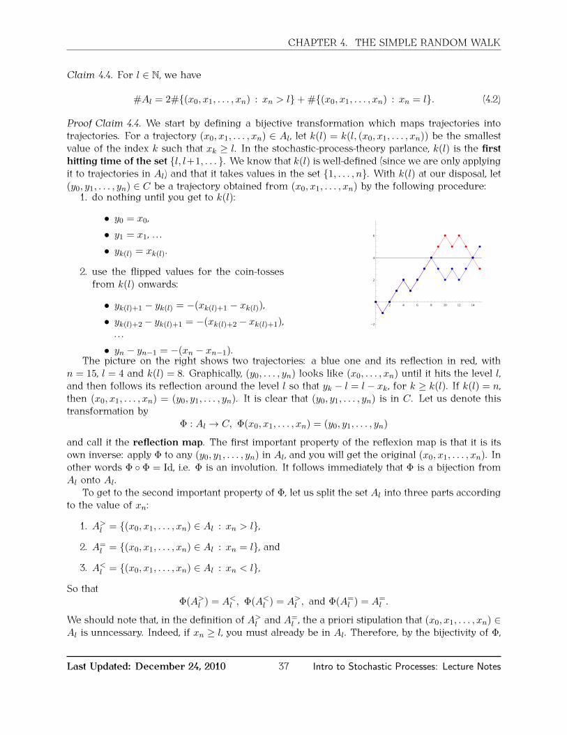
Proof Claim 4.4. We start by defining a bijective transformation which maps trajectories intotrajectories. For a trajectory (x0, x1, . . . , xn) ∈ Al , let k(l) = k(l, (x0, x1, . . . , xn)) be the smallestvalue of the index k such that xk ≥ l. In the stochastic-process-theory parlance, k(l) is the firsthitting time of the set l, l+1, . . . . We know that k(l) is well-defined (since we are only applyingit to trajectories in Al) and that it takes values in the set 1, . . . , n. With k(l) at our disposal, let(y0, y1, . . . , yn) ∈ C be a trajectory obtained from (x0, x1, . . . , xn) by the following procedure:
1. do nothing until you get to k(l):
• y0 = x0,• y1 = x1, . . .• yk(l) = xk(l).
2. use the flipped values for the coin-tossesfrom k(l) onwards:
• yk(l)+1 − yk(l) = −(xk(l)+1 − xk(l)),• yk(l)+2 − yk(l)+1 = −(xk(l)+2 − xk(l)+1),
. . .• yn − yn−1 = −(xn − xn−1).
æ
æ
æ
æ
æ
æ
æ
æ
æ
æ
æ
æ
æ
æ
æ
æ
æ
æ
æ
æ
æ
æ
æ
æ
æ
æ
æ
æ
æ
æ
æ
æ
2 4 6 8 10 12 14
-2
2
4
6
The picture on the right shows two trajectories: a blue one and its reflection in red, withn = 15, l = 4 and k(l) = 8. Graphically, (y0, . . . , yn) looks like (x0, . . . , xn) until it hits the level l,and then follows its reflection around the level l so that yk − l = l − xk , for k ≥ k(l). If k(l) = n,then (x0, x1, . . . , xn) = (y0, y1, . . . , yn). It is clear that (y0, y1, . . . , yn) is in C . Let us denote thistransformation by
Φ : Al → C, Φ(x0, x1, . . . , xn) = (y0, y1, . . . , yn)
and call it the reflection map. The first important property of the reflexion map is that it is itsown inverse: apply Φ to any (y0, y1, . . . , yn) in Al , and you will get the original (x0, x1, . . . , xn). Inother words Φ Φ = Id, i.e. Φ is an involution. It follows immediately that Φ is a bijection fromAl onto Al.
To get to the second important property of Φ, let us split the set Al into three parts accordingto the value of xn:
1. A>l = (x0, x1, . . . , xn) ∈ Al : xn > l,
2. A=l = (x0, x1, . . . , xn) ∈ Al : xn = l, and
3. A<l = (x0, x1, . . . , xn) ∈ Al : xn < l,
So thatΦ(A>l ) = A<l , Φ(A<l ) = A>l , and Φ(A=
l ) = A=l .
We should note that, in the definition of A>l and A=l , the a priori stipulation that (x0, x1, . . . , xn) ∈
Al is unncessary. Indeed, if xn ≥ l, you must already be in Al. Therefore, by the bijectivity of Φ,
Last Updated: December 24, 2010 37 Intro to Stochastic Processes: Lecture Notes

CHAPTER 4. THE SIMPLE RANDOM WALK
we have#A<l = #A>l = #(x0, x1, . . . , xn) : xn > l,
and so#Al = 2#(x0, x1, . . . , xn) : xn > l+ #(x0, x1, . . . , xn) : xn = l,
just as we claimed.
Now that we have (4.2), we can easily rewrite it as follows:
P[Mn ≥ l] = P[Xn = l] + 2∑j>l
P[Xn = j] =∑j>l
P[Xn = j] +∑j≥l
P[Xn = j].
Finally, we subtract P[Mn ≥ l + 1] from P[Mn ≥ l] to get the expression for P[Mn = l]:
P[Mn = l] = P[Xn = l + 1] + P[Xn = l].
It remains to note that only one of the probabilities P[Xn = l + 1] and P[Xn = l] is non-zero,the first one if n and l have different parity and the second one otherwise. In either case thenon-zero probability is given by (
n
bn+l+12 c
)2−n.
Let us use the reflection principle to solve a classical problem in combinatorics.
Example 4.5 (The Ballot Problem). Suppose that two candidates, Daisy and Oscar, are runningfor office, and n ∈ N voters cast their ballots. Votes are counted by the same official, one by one,until all n of them have been processed (like in the old days). After each ballot is opened, theofficial records the number of votes each candidate has received so far. At the end, the officialannounces that Daisy has won by a margin of m > 0 votes, i.e., that Daisy got (n + m)/2 votesand Oscar the remaining (n − m)/2 votes. What is the probability that at no time during thecounting has Oscar been in the lead?
We assume that the order in which the official counts the votes is completely independentof the actual votes, and that each voter chooses Daisy with probability p ∈ (0, 1) and Oscar withprobability q = 1 − p. For k ≤ n, let Xk be the number of votes received by Daisy minus thenumber of votes received by Oscar in the first k ballots. When the k + 1-st vote is counted, Xk
either increases by 1 (if the vote was for Daisy), or decreases by 1 otherwise. The votes areindependent of each other and X0 = 0, so Xk , 0 ≤ k ≤ n is (the beginning of) a simple randomwalk. The probability of an up-step is p ∈ (0, 1), so this random walk is not necessarily symmetric.The ballot problem can now be restated as follows:
What is the probability that Xk ≥ 0 for all k ∈ 0, . . . , n, given that Xn = m?
The first step towards understanding the solution is the realization that the exact value of p doesnot matter. Indeed, we are interested in the conditional probability P[F |G] = P[F∩G]/P[G], whereF denotes the family of all trajectories that always stay non-negative and G the family of those
Last Updated: December 24, 2010 38 Intro to Stochastic Processes: Lecture Notes
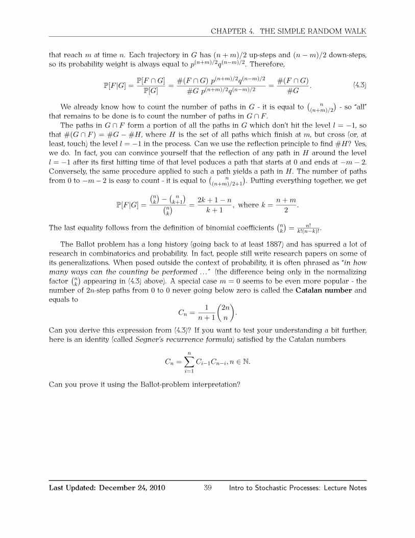
CHAPTER 4. THE SIMPLE RANDOM WALK
that reach m at time n. Each trajectory in G has (n+m)/2 up-steps and (n−m)/2 down-steps,so its probability weight is always equal to p(n+m)/2q(n−m)/2. Therefore,
P[F |G] =P[F ∩G]
P[G]=
#(F ∩G) p(n+m)/2q(n−m)/2
#G p(n+m)/2q(n−m)/2=
#(F ∩G)
#G. (4.3)
We already know how to count the number of paths in G - it is equal to(
n(n+m)/2
)- so “all”
that remains to be done is to count the number of paths in G ∩ F .The paths in G ∩ F form a portion of all the paths in G which don’t hit the level l = −1, so
that #(G ∩ F ) = #G −#H , where H is the set of all paths which finish at m, but cross (or, atleast, touch) the level l = −1 in the process. Can we use the reflection principle to find #H? Yes,we do. In fact, you can convince yourself that the reflection of any path in H around the levell = −1 after its first hitting time of that level poduces a path that starts at 0 and ends at −m− 2.Conversely, the same procedure applied to such a path yields a path in H . The number of pathsfrom 0 to −m− 2 is easy to count - it is equal to
(n
(n+m)/2+1
). Putting everything together, we get
P[F |G] =
(nk
)−(nk+1
)(nk
) =2k + 1− nk + 1
, where k =n+m
2.
The last equality follows from the definition of binomial coefficients(nk
)= n!
k!(n−k)! .
The Ballot problem has a long history (going back to at least 1887) and has spurred a lot ofresearch in combinatorics and probability. In fact, people still write research papers on some ofits generalizations. When posed outside the context of probability, it is often phrased as “in howmany ways can the counting be performed . . . ” (the difference being only in the normalizingfactor
(nk
)appearing in (4.3) above). A special case m = 0 seems to be even more popular - the
number of 2n-step paths from 0 to 0 never going below zero is called the Catalan number andequals to
Cn =1
n+ 1
(2n
n
).
Can you derive this expression from (4.3)? If you want to test your understanding a bit further,here is an identity (called Segner’s recurrence formula) satisfied by the Catalan numbers
Cn =n∑i=1
Ci−1Cn−i, n ∈ N.
Can you prove it using the Ballot-problem interpretation?
Last Updated: December 24, 2010 39 Intro to Stochastic Processes: Lecture Notes

Chapter 5
Generating functions
The path-counting method used in the previous lecture only works for computations related tothe first n steps of the random walk, where n is given in advance. We will see later that mostof the interesting questions do not fall into this category. For example, the distribution of thetime it takes for the random walk to hit the level l 6= 0 is like that. There is no way to givean a-priori bound on the number of steps it will take to get to l (in fact, the expectation of thisrandom variable is +∞). To deal with a wider class of properties of random walks (and otherprocesses), we need to develop some new mathematical tools.
5.1 Definition and first properties
The distribution of an N0-valued random variable X is completely determined by the sequencepnn∈N0 of numbers in [0, 1] given by
pn = P[X = n], n ∈ N0.
As a sequence of real numbers, pnn∈N0 can be used to construct a power series:
PX(s) =∞∑k=0
pksk. (5.1)
It follows from the fact that∑
n |pn| ≤ 1 that the radius of convergence1 of pnn∈N0 is atleast equal to 1. Therefore, PX is well defined for s ∈ [−1, 1], and, perhaps, elsewhere, too.
Definition 5.1. The function PX given by PX(s) =∑∞
k=0 pksk is called the generating function
of the random variable X , or, more precisely, of its pmf pnn∈N0 .
Before we proceed, let us find an expression for the generating functions of some of thepopular N0-valued random variables.
Example 5.2.1Remember, that the radius of convergence of a power series
∑∞k=0 akx
k is the largest number R ∈ [0,∞] suchthat
∑∞k=0 akx
k converges absolutely whenever |x| < R.
40

CHAPTER 5. GENERATING FUNCTIONS
1. Bernoulli - b(p) Here p0 = q, p1 = p, and pn = 0, for n ≥ 2. Therefore,
PX(s) = ps+ q.
2. Binomial - b(n, p) Since pk =(nk
)pkqn−k , k = 0, . . . , n, we have
PX(s) =
n∑k=0
(n
k
)pkqn−ksk = (ps+ q)n,
by the binomial theorem.
3. Geometric - g(p) For k ∈ N0, pk = qkp, so that
PX(s) =
∞∑k=0
qkskp = p
∞∑k=0
(qs)k =p
1− qs.
4. Poisson - p(λ) Given that pk = e−λ λk
k! , k ∈ N0, we have
PX(s) =∞∑k=0
e−λλk
k!sk = e−λ
∞∑k=0
(sλ)k
k!= e−λesλ = eλ(s−1).
Some of the most useful analytic properties of PX are listed in the following proposition
Proposition 5.3. Let X be an N0-valued random variable, let pnn∈N0 be its pmf, and let PXbe its generating function. Then
1. PX(s) = E[sX ], s ∈ [−1, 1],
2. PX(s) is convex and non-decreasing with 0 ≤ PX(s) ≤ 1 for s ∈ [0, 1]
3. PX(s) is infinitely differentiable on (−1, 1) with
dn
dsnPX(s) =
∞∑k=n
k(k − 1) . . . (k − n+ 1)sk−npk, n ∈ N. (5.2)
In particular, pn = 1n!
dn
dsnPX(s)∣∣s=0
and so s 7→ PX(s) uniquely determines the sequencepnn∈N0 .
Proof. Statement (1) follows directly from the formula E[g(X)] =∑∞
k=0 g(k)pk , applied to g(x) =sx. As far as (3) is concerned, we only note that the expression (5.2) is exactly what you wouldget if you differentiated the expression (5.1) term by term. The rigorous proof of the fact this isallowed is beyond the scope of these notes. With (3) at our disposal, (2) follows by the fact thatthe first two derivatives of the function PX are non-negative and that PX(1) = 1.
Remark 5.4.
1. If you know about moment-generating functions, you will notice that PX(s) = MX(log(s)),for s ∈ (0, 1), where MX(λ) = E[exp(λX)] is the moment-generating function of X .
Last Updated: December 24, 2010 41 Intro to Stochastic Processes: Lecture Notes

CHAPTER 5. GENERATING FUNCTIONS
2. Generating functions can be used with sequences ann∈N0 which are not necessarily pmf’sof random variables. The method is useful for any sequence ann∈N0 such that the powerseries
∑∞k=0 aks
k has a positive (non-zero) radius of convergence.
3. The name generating function comes from the last part of the property (3). The knowledgeof PX implies the knowledge of the whole sequence pnn∈N0 . Put differently, PX generatesthe whole distribution of X .
Remark 5.5. Note that the true radius of convergence varies from distribution to distribution. Itis infinite in (1), (2) and (4), and equal to 1/q > 1 in (3), in Example 5.2. For the distribution withpmf given by pk = C
(k+1)2, where C = (
∑∞k=0
1(k+1)2
)−1, the radius of convergence is exactly equalto 1. Can you see why?
5.2 Convolution and moments
The true power of generating functions comes from the fact that they behave very well underthe usual operations in probability.
Definition 5.6. Let pnn∈N0 and qnn∈N0 be two probability-mass functions. The convolutionp ∗ q of pnn∈N0 and qnn∈N0 is the sequence rnn∈N0 , where
rn =n∑k=0
pkqn−k, n ∈ N0.
This abstractly-defined operation will become much clearer once we prove the followingproposition:
Proposition 5.7. Let X,Y be two independent N0-valued random variables with pmfs pnn∈N0
and qnn∈N0 . Then the sum Z = X + Y is also N0-valued and its pmf is the convolution ofpnn∈N0 and qnn∈N0 in the sense of Definition 5.6.
Proof. Clearly, Z is N0-valued. To obtain an expression for its pmf, we use the law of totalprobability:
P[Z = n] =n∑k=0
P[X = k]P[Z = n|X = k].
However, P[Z = n|X = k] = P[X + Y = n|X = k] = P[Y = n − k|X = k] = P[Y = n − k], wherethe last equality follows from independence of X and Y . Therefore,
P[Z = n] =n∑k=0
P[X = k]P[Y = n− k] =n∑k=0
pkqn−k.
Corollary 5.8. Let pnn∈N0 and pnn∈N0 be any two pmfs.
1. Convolution is commutative, i.e., p ∗ q = q ∗ p.
Last Updated: December 24, 2010 42 Intro to Stochastic Processes: Lecture Notes

CHAPTER 5. GENERATING FUNCTIONS
2. The convolution of two pmfs is a pmf, i.e. rn ≥ 0, for all n ∈ N0 and∑∞
k=0 rk = 1, forr = p ∗ q.
Corollary 5.9. Let pnn∈N0 and pnn∈N0 be any two pmfs, and let
P (s) =∞∑k=0
pksk and Q(s) =
∞∑k=0
qksk
be their generating functions. Then the generating function R(s) =∑∞
k=0 rksk , of the convolu-
tion r = p ∗ q is given byR(s) = P (s)Q(s).
Equivalently, the generating function PX+Y of the sum of two independent N0-valued randomvariables is equal to the product
PX+Y (s) = PX(s)PY (s),
of the generating functions PX and PY of X and Y .
Example 5.10.
1. The binomial b(n, p) distribution is a sum of n independent Bernoullis b(p). Therefore,if we apply Corrolary 5.9 n times to the generating function (q + ps) of the Bernoullib(p) distribution we immediately get that the generating function of the binomial is (q +ps) . . . (q + ps) = (q + ps)n.
2. More generally, we can show that the sum of m independent random variables with theb(n, p) distribution has a binomial distribution b(mn, p). If you try to sum binomials withdifferent values of the parameter p you will not get a binomial.
3. What is even more interesting, the following statement can be shown: Suppose that thesum Z of two independent N0-valued random variables X and Y is binomially distributedwith parameters n and p. Then both X and Y are binomial with parameters nX , p andny, p where nX + nY = n. In other words, the only way to get a binomial as a sum ofindependent random variables is the trivial one.
Another useful thing about generating functions is that they make the computation of mo-ments easier.
Proposition 5.11. Let pnn∈N0 be a pmf of an N0-valued random variable X and let P (s) beits generating function. For n ∈ N the following two statements are equivalent
1. E[Xn] <∞,
2. dnP (s)dsn
∣∣∣s=1
exists (in the sense that the left limit lims1dnP (s)dsn exists)
In either case, we have
E[X(X − 1)(X − 2) . . . (X − n+ 1)] =dn
dsnP (s)
∣∣∣s=1
.
Last Updated: December 24, 2010 43 Intro to Stochastic Processes: Lecture Notes

CHAPTER 5. GENERATING FUNCTIONS
The quantitiesE[X], E[X(X − 1)], E[X(X − 1)(X − 2)], . . .
are called factorial moments of the random variable X . You can get the classical moments fromthe factorial moments by solving a system of linear equations. It is very simple for the first few:
E[X] = E[X],
E[X2] = E[X(X − 1)] + E[X],
E[X3] = E[X(X − 1)(X − 2)]] + 3E[X(X − 1)] + E[X], . . .
A useful identity which follows directly from the above results is the following:
Var[X] = P ′′(1) + P ′(1)− (P ′(1))2,
and it is valid if the first two derivatives of P at 1 exist.
Example 5.12. Let X be a Poisson random variable with parameter λ. Its generating function isgiven by
PX(s) = eλ(s−1).
Therefore, dn
dsnPX(1) = λn, and so, the sequence (E[X],E[X(X − 1)],E[X(X − 1)(X − 2)], . . . ) offactorial moments of X is just (λ, λ2, λ3, . . . ). It follows that
E[X] = λ,
E[X2] = λ2 + λ, Var[X] = λ
E[X3] = λ3 + 3λ2 + λ, . . .
5.3 Random sums and Wald’s identity
Our next application of generating function in the theory of stochastic processes deals with theso-called random sums. Let ξnn∈N be a sequence of random variables, and let N be a randomtime (a random time is simply an N0∪+∞-value random variable). We can define the randomvariable
Y =
N∑k=0
ξk by Y (ω) =
0, N(ω) = 0,∑N(ω)
k=1 ξk(ω), N(ω) ≥ 1for ω ∈ Ω.
More generally, for an arbitrary stochastic process Xnn∈N0 and a random time N (with P[N =+∞] = 0), we define the random variable XN by XN (ω) = XN(ω)(ω), for ω ∈ Ω. When Nis a constant (N = n), then XN is simply equal to Xn. In general, think of XN as a valueof the stochasti process X taken at the time which is itself random. If Xn =
∑nk=1 ξk , then
XN =∑N
k=1 ξk .
Example 5.13. Let ξnn∈N be the increments of a symmetric simple random walk (coin-tosses),and let N have the following distribution
N ∼(
0 1 21/3 1/3 1/3
)
Last Updated: December 24, 2010 44 Intro to Stochastic Processes: Lecture Notes
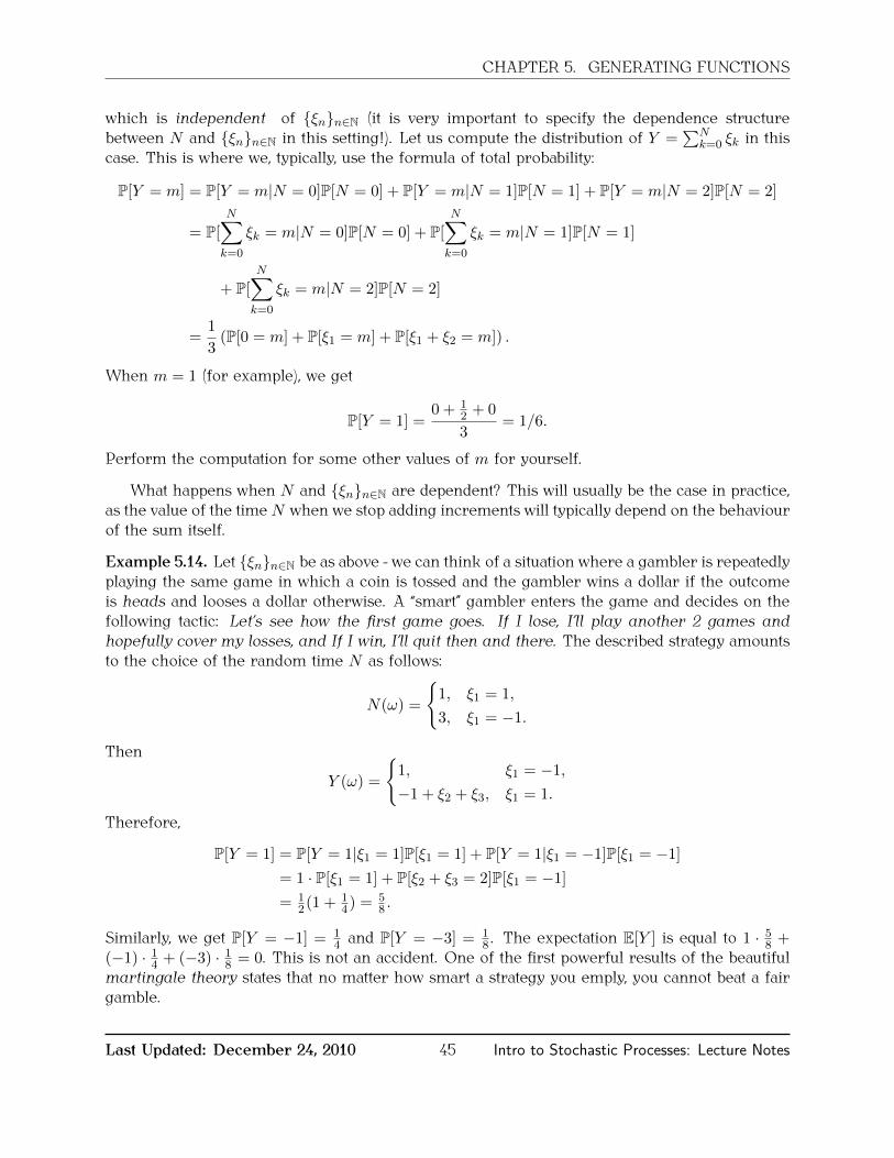
CHAPTER 5. GENERATING FUNCTIONS
which is independent of ξnn∈N (it is very important to specify the dependence structurebetween N and ξnn∈N in this setting!). Let us compute the distribution of Y =
∑Nk=0 ξk in this
case. This is where we, typically, use the formula of total probability:
P[Y = m] = P[Y = m|N = 0]P[N = 0] + P[Y = m|N = 1]P[N = 1] + P[Y = m|N = 2]P[N = 2]
= P[
N∑k=0
ξk = m|N = 0]P[N = 0] + P[
N∑k=0
ξk = m|N = 1]P[N = 1]
+ P[N∑k=0
ξk = m|N = 2]P[N = 2]
=1
3(P[0 = m] + P[ξ1 = m] + P[ξ1 + ξ2 = m]) .
When m = 1 (for example), we get
P[Y = 1] =0 + 1
2 + 0
3= 1/6.
Perform the computation for some other values of m for yourself.
What happens when N and ξnn∈N are dependent? This will usually be the case in practice,as the value of the time N when we stop adding increments will typically depend on the behaviourof the sum itself.
Example 5.14. Let ξnn∈N be as above - we can think of a situation where a gambler is repeatedlyplaying the same game in which a coin is tossed and the gambler wins a dollar if the outcomeis heads and looses a dollar otherwise. A “smart” gambler enters the game and decides on thefollowing tactic: Let’s see how the first game goes. If I lose, I’ll play another 2 games andhopefully cover my losses, and If I win, I’ll quit then and there. The described strategy amountsto the choice of the random time N as follows:
N(ω) =
1, ξ1 = 1,
3, ξ1 = −1.
Then
Y (ω) =
1, ξ1 = −1,
−1 + ξ2 + ξ3, ξ1 = 1.
Therefore,
P[Y = 1] = P[Y = 1|ξ1 = 1]P[ξ1 = 1] + P[Y = 1|ξ1 = −1]P[ξ1 = −1]
= 1 · P[ξ1 = 1] + P[ξ2 + ξ3 = 2]P[ξ1 = −1]
= 12(1 + 1
4) = 58 .
Similarly, we get P[Y = −1] = 14 and P[Y = −3] = 1
8 . The expectation E[Y ] is equal to 1 · 58 +(−1) · 14 + (−3) · 18 = 0. This is not an accident. One of the first powerful results of the beautifulmartingale theory states that no matter how smart a strategy you emply, you cannot beat a fairgamble.
Last Updated: December 24, 2010 45 Intro to Stochastic Processes: Lecture Notes
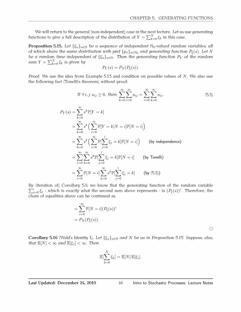
CHAPTER 5. GENERATING FUNCTIONS
We will return to the general (non-independent) case in the next lecture. Let us use generatingfunctions to give a full description of the distribution of Y =
∑Nk=0 ξk in this case.
Proposition 5.15. Let ξnn∈N be a sequence of independent N0-valued random variables, allof which share the same distribution with pmf pnn∈N0 and generating function Pξ(s). Let Nbe a random time independent of ξnn∈N. Then the generating function PY of the randomsum Y =
∑Nk=0 ξk is given by
PY (s) = PN (Pξ(s)).
Proof. We use the idea from Example 5.13 and condition on possible values of N . We also usethe following fact (Tonelli’s theorem) without proof:
If ∀ i, j aij ≥ 0, then∞∑k=0
∞∑i=0
aij =∞∑i=0
∞∑k=0
aij . (5.3)
PY (s) =∞∑k=0
skP[Y = k]
=∞∑k=0
sk( ∞∑i=0
P[Y = k|N = i]P[N = i])
=∞∑k=0
sk( ∞∑i=0
P[i∑
j=0
ξj = k]P[N = i])
(by independence)
=∞∑i=0
∞∑k=0
skP[i∑
j=0
ξj = k]P[N = i] (by Tonelli)
=
∞∑i=0
P[N = i]
∞∑k=0
skP[
i∑j=0
ξj = k] (by (5.3))
By (iteration of) Corollary 5.9, we know that the generating function of the random variable∑ij=0 ξj - which is exactly what the second sum above represents - is (Pξ(s))
i. Therefore, thechain of equalities above can be continued as
=
∞∑i=0
P[N = i](Pξ(s))i
= PN (Pξ(s)).
Corollary 5.16 (Wald’s Identity I). Let ξnn∈N and N be as in Proposition 5.15. Suppose, also,that E[N ] <∞ and E[ξ1] <∞. Then
E[
N∑k=0
ξk] = E[N ]E[ξ1].
Last Updated: December 24, 2010 46 Intro to Stochastic Processes: Lecture Notes

CHAPTER 5. GENERATING FUNCTIONS
Proof. We just apply the composition rule for derivatives to the equality PY = PN Pξ to get
P ′Y (s) = P ′N (Pξ(s))P′ξ(s).
After we let s 1, we get
E[Y ] = P ′Y (1) = P ′N (Pξ(1))P ′ξ(1) = P ′N (1)P ′ξ(1) = E[N ]E[ξ1].
Example 5.17. Every time Springfield Wildcats play in the Superbowl, their chance of winningis p ∈ (0, 1). The number of years between two Superbowls they get to play in has the Poissondistribution p(λ), λ > 0. What is the expected number of years Y between the consequtiveSuperbowl wins?
Let ξnn∈N be the sequence of independent p(λ)-random variables modeling the numberof years between consecutive Superbowl appearances by the Wildcat. Moreover, let N be ageometric g(p) random variable with success probability p. Then
Y =N∑k=0
ξk.
Indeed, every time the Wildcats lose the Superbowl, another ξ· years have to pass before theyget another chance and the whole thing stops when they finally win. To compute the expectationof Y we use Corollary 5.16
E[Y ] = E[N ]E[ξk] =1− pp
λ.
Last Updated: December 24, 2010 47 Intro to Stochastic Processes: Lecture Notes

Chapter 6
Random walks - advanced methods
6.1 Stopping times
The last application of generating functions dealt with sums evaluated between 0 and somerandom time N . An especially interesting case occurs when the value of N depends directlyon the evolution of the underlying stochastic process. Even more important is the case wheretime’s arrow is taken into account. If you think of N as the time you stop adding new terms tothe sum, it is usually the case that you are not allowed (able) to see the values of the terms youwould get if you continued adding. Think of an investor in the stock market. Her decision tostop and sell her stocks can depend only on the information available up to the moment of thedecision. Otherwise, she would sell at the absolute maximum and buy at the absolute minimum,making tons of money in the process. Of course, this is not possible unless you are clairvoyant,so the mere mortals have to restrict their choices to so-called stopping times.Definition 6.1. Let Xnn∈N0 be a stochastic process. A random variable T taking values inN0∪+∞ is said to be a stopping time with respect to Xnn∈N0 if for each n ∈ N0 there existsa function Gn : Rn+1 → 0, 1 such that
1T=n = Gn(X0, X1, . . . , Xn), for all n ∈ N0.
The functions Gn are called the decision functions, and should be thought of as a black boxwhich takes the values of the process Xnn∈N0 observed up to the present point and outputseither 0 or 1. The value 0 means keep going and 1 means stop. The whole point is that thedecision has to based only on the available observations and not on the future ones.Example 6.2.
1. The simplest examples of stopping times are (non-random) deterministic times. Just setT = 5 (or T = 723 or T = n0 for any n0 ∈ N0 ∪ +∞), no matter what the state of theworld ω ∈ Ω is. The family of decision rules is easy to construct:
Gn(x0, x1, . . . , xn) =
1, n = n0,
0, n 6= n0..
Decision functions Gn do not depend on the values of X0, X1, . . . , Xn at all. A gamblerwho stops gambling after 20 games, no matter of what the winnings of losses are uses sucha rule.
48

CHAPTER 6. RANDOM WALKS - ADVANCED METHODS
2. Probably the most well-known examples of stopping times are (first) hitting times. Theycan be defined for general stochastic processes, but we will stick to simple random walksfor the purposes of this example. So, let Xn =
∑nk=0 ξk be a simple random walk, and let
Tl be the first time X hits the level l ∈ N. More precisely, we use the following slightlynon-intuitive but mathematically correct definition
Tl = minn ∈ N0 : Xn = l.
The set n ∈ N0 : Xn = l is the collection of all time-points at which X visits the level l.The earliest one - the minimum of that set - is the first hitting time of l. In states of theworld ω ∈ Ω in which the level l just never get reached, i.e., when n ∈ N0 : Xn = l is anempty set, we set Tl(ω) = +∞. In order to show that Tl is indeed a stopping time, we needto construct the decision functions Gn, n ∈ N0. Let us start with n = 0. We would haveTl = 0 in the (impossible) case X0 = l, so we always have G0(X0) = 0. How about n ∈ N.For the value of Tl to be equal to exactly n, two things must happen:
(a) Xn = l (the level l must actually be hit at time n), and(b) Xn−1 6= l, Xn−2 6= l, . . . , X1 6= l, X0 6= l (the level l has not been hit before).
Therefore,
Gn(x0, x1, . . . , xn) =
1, x0 6= l, x1 6= l, . . . , xn−1 6= l, xn = l
0, otherwise.
The hitting time T2 of the level l = 2 for a particular trajectory of a symmetric simplerandom walk is depicted below:
T2 TM5 10 15 20 25 30
-6
-4
-2
2
4
6
.
3. How about something that is not a stopping time? Let n0 be an arbitrary time-horizon andlet TM be the last time during 0, . . . , n0 that the random walk visits its maximum during0, . . . , n0 (see picture above). If you bought a stock at time t = 0, had to sell it some timebefore n0 and had the ability to predict the future, this is one of the points you would chooseto sell it at. Of course, it is impossible to decide whether TM = n, for some n ∈ 0, . . . , n0−1without the knowledge of the values of the random walk after n. More precisely, let ussketch the proof of the fact that TM is not a stopping time. Suppose, to the contrary, that itis, and let Gn be the family of decision functions. Consider the following two trajectories:(0, 1, 2, 3, . . . , n− 1, n) and (0, 1, 2, 3, . . . , n− 1, n− 2). The differ only in the direction of the
Last Updated: December 24, 2010 49 Intro to Stochastic Processes: Lecture Notes

CHAPTER 6. RANDOM WALKS - ADVANCED METHODS
last step. They also differ in the fact that TM = n for the first one and TM = n− 1 for thesecond one. On the other hand, by the definition of the decision functions, we have
1TM=n−1 = Gn−1(X0, . . . , Xn−1).
The right-hand side is equal for both trajectories, while the left-hand side equals to 0 forthe first one and 1 for the second one. A contradiction.
6.2 Wald’s identity II
Having defined the notion of a stopping time, let use try to compute something about it. Therandom variables ξnn∈N in the statement of the theorem below are only assumed to be in-dependent of each other and identically distributed. To make things simpler, you can think ofξnn∈N as increments of a simple random walk. Before we state the main result, here is anextremely useful identity:
Proposition 6.3. Let N be an N0-valued random variable. Then
E[N ] =∞∑k=1
P[N ≥ k].
Proof. Clearly, P[N ≥ k] =∑
j≥k P[N = j], so (note what happens to the indices when we switchthe sums)
∞∑k=1
P[N ≥ k] =∞∑k=1
∑j≥k
P[N = j]
=∞∑j=1
j∑k=1
P[n = j] =∞∑j=1
jP[N = j]
= E[N ].
Theorem 6.4 (Wald’s Identity II). Let ξnn∈N be a sequence of independent, identically dis-tributed random variables with E[|ξ1|] <∞. Set
Xn =
n∑k=1
ξk, n ∈ N0.
If T is an Xnn∈N0 -stopping time such that E[T ] <∞, then
E[XT ] = E[ξ1]E[T ].
Proof. Here is another way of writing the sum∑T
k=1 ξk :
T∑k=1
ξk =
∞∑k=1
ξk1k≤T.
Last Updated: December 24, 2010 50 Intro to Stochastic Processes: Lecture Notes

CHAPTER 6. RANDOM WALKS - ADVANCED METHODS
The idea behind it is simple: add all the values of ξk for k ≤ T and keep adding zeros (sinceξk1k≤T = 0 for k > T ) after that. Taking expectation of both sides and switching E and
∑(this
can be justified, but the argument is technical and we omit it here) yields:
E[T∑k=1
ξk] =∞∑k=1
E[1k≤Tξk]. (6.1)
Let us examine the term E[ξk1k≤T] in some detail. We first note that
1k≤T = 1− 1k>T = 1− 1k−1≥T = 1−k−1∑j=0
1T=j.
Therefore,
E[ξk1k≤T] = E[ξk]−k−1∑j=0
E[ξk1T=j].
By the assumption that T is a stopping time, the indicator 1T=j can be represented as 1T=j =Gj(X0, . . . , Xj), and, because each Xi is just a sum of the increments, we can actually write 1T=jas a function of ξ1, . . . , ξj only - say 1T=j = Hj(ξ1, . . . , ξj). By the independence of (ξ1, . . . , ξj)from ξk (because j < k) we have
E[ξk1T=j] = E[ξkHj(ξ1, . . . , ξj)] = E[ξk]E[Hj(ξ1, . . . , ξj)] = E[ξk]E[1T=j] = E[ξk]P[T = j].
Therefore,
E[ξk1k≤T] = E[ξk]−k−1∑j=0
E[ξk]P[T = j] = E[ξk]P[T ≥ k] = E[ξ1]P[T ≥ k],
where the last equality follows from the fact that all ξk have the same distribution.Going back to (6.1), we get
E[XT ] = E[
T∑k=1
ξk] =
∞∑k=1
E[ξ1]P[T ≥ k] = E[ξ1]
∞∑k=1
P[T ≥ k] = E[ξ1]E[T ],
where we use Proposition 6.3 for the last equality.
Example 6.5 (Gambler’s ruin problem). . A gambler start with x ∈ N dollars and repeatedly playsa game in which he wins a dollar with probability 1
2 and loses a dollar with probability 12 . He
decides to stop when one of the following two things happens:
1. he goes bankrupt, i.e., his wealth hits 0, or
2. he makes enough money, i.e., his wealth reaches some level a > x.
The classical “Gambler’s ruin” problem asks the following question: what is the probability thatthe gambler will make a dollars before he goes bankrupt?
Last Updated: December 24, 2010 51 Intro to Stochastic Processes: Lecture Notes
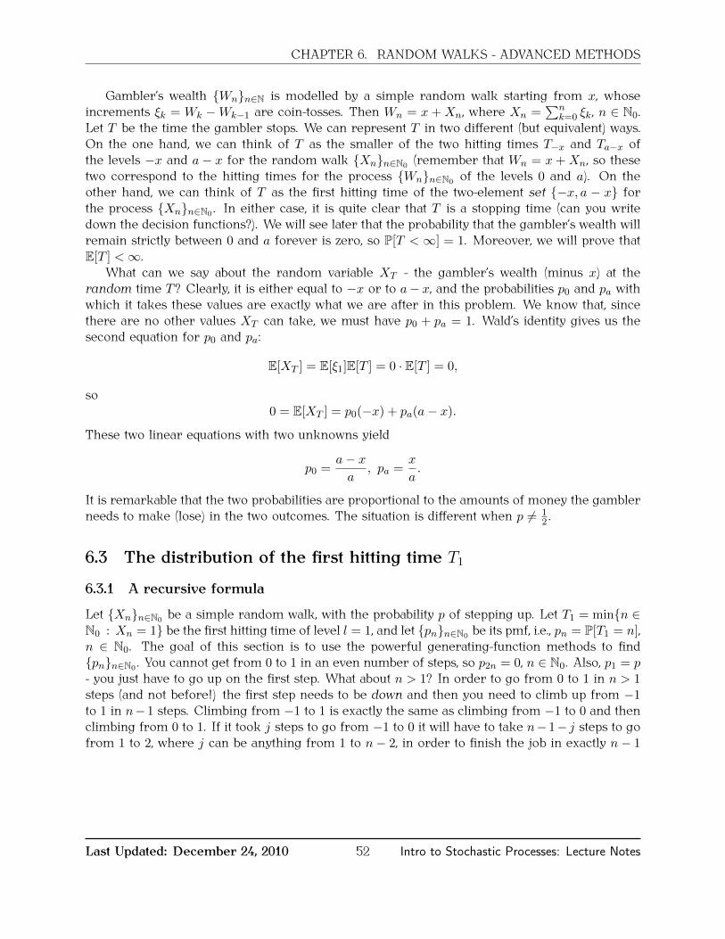
CHAPTER 6. RANDOM WALKS - ADVANCED METHODS
Gambler’s wealth Wnn∈N is modelled by a simple random walk starting from x, whoseincrements ξk = Wk −Wk−1 are coin-tosses. Then Wn = x + Xn, where Xn =
∑nk=0 ξk , n ∈ N0.
Let T be the time the gambler stops. We can represent T in two different (but equivalent) ways.On the one hand, we can think of T as the smaller of the two hitting times T−x and Ta−x ofthe levels −x and a− x for the random walk Xnn∈N0 (remember that Wn = x+Xn, so thesetwo correspond to the hitting times for the process Wnn∈N0 of the levels 0 and a). On theother hand, we can think of T as the first hitting time of the two-element set −x, a − x forthe process Xnn∈N0 . In either case, it is quite clear that T is a stopping time (can you writedown the decision functions?). We will see later that the probability that the gambler’s wealth willremain strictly between 0 and a forever is zero, so P[T < ∞] = 1. Moreover, we will prove thatE[T ] <∞.
What can we say about the random variable XT - the gambler’s wealth (minus x) at therandom time T ? Clearly, it is either equal to −x or to a− x, and the probabilities p0 and pa withwhich it takes these values are exactly what we are after in this problem. We know that, sincethere are no other values XT can take, we must have p0 + pa = 1. Wald’s identity gives us thesecond equation for p0 and pa:
E[XT ] = E[ξ1]E[T ] = 0 · E[T ] = 0,
so0 = E[XT ] = p0(−x) + pa(a− x).
These two linear equations with two unknowns yield
p0 =a− xa
, pa =x
a.
It is remarkable that the two probabilities are proportional to the amounts of money the gamblerneeds to make (lose) in the two outcomes. The situation is different when p 6= 1
2 .
6.3 The distribution of the first hitting time T1
6.3.1 A recursive formula
Let Xnn∈N0 be a simple random walk, with the probability p of stepping up. Let T1 = minn ∈N0 : Xn = 1 be the first hitting time of level l = 1, and let pnn∈N0 be its pmf, i.e., pn = P[T1 = n],n ∈ N0. The goal of this section is to use the powerful generating-function methods to findpnn∈N0 . You cannot get from 0 to 1 in an even number of steps, so p2n = 0, n ∈ N0. Also, p1 = p- you just have to go up on the first step. What about n > 1? In order to go from 0 to 1 in n > 1steps (and not before!) the first step needs to be down and then you need to climb up from −1to 1 in n− 1 steps. Climbing from −1 to 1 is exactly the same as climbing from −1 to 0 and thenclimbing from 0 to 1. If it took j steps to go from −1 to 0 it will have to take n− 1− j steps to gofrom 1 to 2, where j can be anything from 1 to n− 2, in order to finish the job in exactly n− 1
Last Updated: December 24, 2010 52 Intro to Stochastic Processes: Lecture Notes

CHAPTER 6. RANDOM WALKS - ADVANCED METHODS
steps. So, in formulas, we have
P[T1 = n] =
= qn−2∑j=1
P[“exactly j steps to first hit 0 from −1” and “exactly n− 1− j steps to first hit 1 from 0”].
(6.2)
Taking j steps from −1 to 0 is exactly the same as taking j steps from 0 to 1, so
P[“exactly j steps to first hit 0 from −1”] = P[T1 = j] = pj .
By the same token,
P[“exactly n− 1− j steps to first hit 1 from 0”] = P[T1 = n− 1− j] = pn−1−j .
Finally, I claim that the two events are independent of each other1. Indeed, once we have reached0, the future increments of the random walk behave exactly the same as the increments of a freshrandom walk starting from zero - they are independent of everything. Equivalently, a knowledgeof everything that happened until the moment the random walk hit 0 for the first time doesnot change our perception (and estimation) of what is going to happen later - in this case thelikelihood of hitting 1 in exactly n−1−j steps. This property is called the regeneration propertyor the strong Lévy property of random walks. More precisely (but still not entirely precise), wecan make the following claim:
Let Xnn∈N0 be a simple random walk and let T be any N0-valued stopping time.Define the process Ynn∈N0 by Yn = XT+n − XT . Then Ynn∈N0 is also a simplerandom walk, and it is independent of X up to T .
In order to check your understanding, try to convince yourself that the requirement that T be astopping time is necessary - find an example of a random time T which is not a stopping timewhere the statement above fails.
We can go back to the distribution of the hitting time T1, and use our newly-found indepen-dence together with (6.2) to obtain the following recursion
pn = qn−2∑j=1
pjpn−j−1, n > 1, p0 = 0, p1 = p. (6.3)
6.3.2 Generating-function approach
This is where generating functions step in. We will use (6.3) to derive an equation for thegenerating function P (s) =
∑∞k=0 pks
k . The sum on the right-hand side of (6.3) looks a little bitlike a convolution, so let us compare it to the following expansion of the square P (s)2:
P (s)2 =
∞∑k=0
(
k∑i=0
pipk−i)sk.
1A demanding reader will object at this point, since my definitions of the two events are somewhat loose. I begforgiveness.
Last Updated: December 24, 2010 53 Intro to Stochastic Processes: Lecture Notes

CHAPTER 6. RANDOM WALKS - ADVANCED METHODS
The inner sum∑k
i=0 pipk−i needs to be split into several parts to get an expression which matches(6.3):
k∑i=0
pipk−i = p0pk︸︷︷︸0
+
k−1∑i=1
pipk−i + pkp0︸︷︷︸0
=
(k+1)−2∑i=1
pip(k+1)−i−1 = q−1pk+1, k ≥ 2.
Therefore, since the coefficients of P (s)2 start at s2, we have
qsP (s)2 = qs∞∑k=2
q−1pk+1sk =
∞∑k=2
pk+1sk+1 = P (s)− ps,
which is nothing but a quadratic equation for P . It admits two solutions (for each s):
P (s) =1±
√1− 4pqs2
2qs.
One of the two solutions is always greater than 1 in absolute value, so it cannot correspond to avalue of a generating function, so we conclude that
P (s) =1−
√1− 4pqs2
2qs, for |s| ≤ 1
2√pq.
It remains to extract the information about pnn∈N0 from P . The obvious way to do it is tocompute higher and higher derivatives of P and s = 1. There is an easier way, though. Thesquare root appearing in the formula for P is an expression of the form (1 + x)1/2 and the(generalized) binomial formula can be used:
(1 + x)α =
∞∑k=0
(α
k
)xα, where
(α
k
)=α(α− 1) . . . (α− k + 1)
k!, k ∈ N, α ∈ R.
Therefore,
P (s) =1
2qs− 1
2qs
∞∑k=0
1
2q
(1/2
k
)(−4pqs2)k =
∞∑k=1
s2k−11
2p(4pq)k(−1)k−1
(1/2
k
), (6.4)
and sop2k−1 =
1
2q(4pq)k(−1)k−1
(1/2
k
), p2k−2 = 0, k ∈ N.
This expression can be simplified a bit further: the formula for(1/2k
)evaluates to:(
1/2
k
)= (−1)k−1
1
4k−11
k
(2k − 3
k − 2
).
Thus,p2k−1 = pkqk−1
2
k
(2k − 3
k − 2
).
This last expression might remind you of something related to the reflection principle. And it is!Can you derive the formula for p2k−1 from the reflection principle? How would you deal withthe fact that the random walk here is not symmetric?
Last Updated: December 24, 2010 54 Intro to Stochastic Processes: Lecture Notes
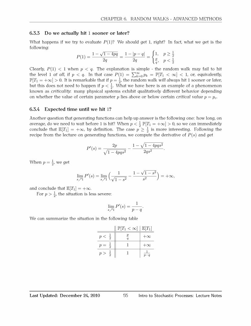
CHAPTER 6. RANDOM WALKS - ADVANCED METHODS
6.3.3 Do we actually hit 1 sooner or later?
What happens if we try to evaluate P (1)? We should get 1, right? In fact, what we get is thefollowing:
P (1) =1−√
1− 4pq
2q=
1− |p− q|2q
=
1, p ≥ 1
2pq , p < 1
2
Clearly, P (1) < 1 when p < q. The explanation is simple - the random walk may fail to hitthe level 1 at all, if p < q. In that case P (1) =
∑∞k=0 pk = P[T1 < ∞] < 1, or, equivalently,
P[T1 = +∞] > 0. It is remarkable that if p = 12 , the random walk will always hit 1 sooner or later,
but this does not need to happen if p < 12 . What we have here is an example of a phenomenon
known as criticality: many physical systems exhibit qualitatively different behavior dependingon whether the value of certain parameter p lies above or below certain critical value p = pc.
6.3.4 Expected time until we hit 1?
Another question that generating functions can help up answer is the following one: how long, onaverage, do we need to wait before 1 is hit? When p < 1
2 P[T1 = +∞] > 0, so we can immediatelyconclude that E[T1] = +∞, by definition. The case p ≥ 1
2 is more interesting. Following therecipe from the lecture on generating functions, we compute the derivative of P (s) and get
P ′(s) =2p√
1− 4pqs2− 1−
√1− 4pqs2
2qs2.
When p = 12 , we get
lims1
P ′(s) = lims1
( 1√1− s2
− 1−√
1− s2s2
)= +∞,
and conclude that E[T1] = +∞.For p > 1
2 , the situation is less severe:
lims1
P ′(s) =1
p− q.
We can summarize the situation in the following table
P[T1 <∞] E[T1]
p < 12
pq +∞
p = 12 1 +∞
p > 12 1 1
p−q
Last Updated: December 24, 2010 55 Intro to Stochastic Processes: Lecture Notes

Chapter 7
Branching processes
7.1 A bit of historyIn the mid 19th century several aristocratic families in VictorianEngland realized that their family names could become extinct.Was it just unfounded paranoia, or did something real promptthem to come to this conclusion? They decided to ask around,and Sir Francis Galton (a “polymath, anthropologist, eugenicist,tropical explorer, geographer, inventor, meteorologist, proto-geneticist, psychometrician and statistician” and half-cousin ofCharles Darwin) posed the following question (1873, Educa-tional Times):
How many male children (on average) must eachgeneration of a family have in order for the familyname to continue in perpetuity?
The first complete answer came from Reverend Henry WilliamWatson soon after, and the two wrote a joint paper entitled Onethe probability of extinction of families in 1874. By the end ofthis lecture, you will be able to give a precise answer to Galton’squestion.
Sir Francis Galton
7.2 A mathematical model
The model proposed by Watson was the following:
1. A population starts with one individual at time n = 0: Z0 = 1.
2. After one unit of time (at time n = 1) the sole individual produces Z1 identical clones ofitself and dies. Z1 is an N0-valued random variable.
3. (a) If Z1 happens to be equal to 0 the population is dead and nothing happens at any futuretime n ≥ 2.
56

CHAPTER 7. BRANCHING PROCESSES
(b) If Z1 > 0, a unit of time later, each of Z1 individuals gives birth to a random numberof children and dies. The first one has Z1,1 children, the second one Z1,2 children,etc. The last, Zth1 one, gives birth to Z1,Z1 children. We assume that the distributionof the number of children is the same for each individual in every generation andindependent of either the number of individuals in the generation and of the numberof children the others have. This distribution, shared by all Zn,i and Z1, is called theoffspring distribution. The total number of individuals in the second generation isnow
Z2 =
Z1∑k=1
Z1,k.
(c) The third, fourth, etc. generations are produced in the same way. If it ever happens thatZn = 0, for some n, then Zm = 0 for all m ≥ n - the population is extinct. Otherwise,
Zn+1 =
Zn∑k=1
Zn,k.
Definition 7.1. A stochastic process with the properties described in (1), (2) and (3) above is calleda (simple) branching process.
The mechanism that produces the next generation from the present one can differ from ap-plication to application. It is the offspring distribution alone that determines the evolution of abranching process. With this new formalism, we can pose Galton’s question more precisely:
Under what conditions on the offspring distribution will the process Znn∈N0 nevergo extinct, i.e., when does
P[Zn ≥ 1 for all n ∈ N0] = 1 (7.1)
hold?
7.3 Construction and simulation of branching processes
Before we answer Galton’s question, let us figure out how to simulate a branching process, for agiven offspring distribution pnn∈N0 (pk = P[Z1 = k]). The distribution pnn∈N0 is N0-valued -we have learned how to simulate such distributions in Lecture 3. We can, therefore, assume thata transformation function F is known, i.e., that the random variable η = F (γ) is N0-valued withpmf pnn∈N0 , where γ ∼ U [0, 1].
Some time ago we assumed that a probability space with a sequence γnn∈N0 of independentU [0, 1] random variables is given. We think of γnn∈N0 as a sequence of random numbersproduced by a computer. Let us first apply the function F to each member of γnn∈N0 to obtainan independent sequence ηnn∈N0 of N0-valued random variables with pmf pnn∈N0 . In thecase of a simple random walk, we would be done at this point - an accumulation of the first nelements of ηnn∈N0 would give you the value Xn of the random walk at time n. Branchingprocesses are a bit more complicated; the increment Zn+1 − Zn depends on Zn: the more
Last Updated: December 24, 2010 57 Intro to Stochastic Processes: Lecture Notes

CHAPTER 7. BRANCHING PROCESSES
individuals in a generation, the more offspring they will produce. In other words, we need ablack box with two inputs - “randomness” and Zn - which will produce Zn+1. What do we meanby “randomness”? Ideally, we would need exactly Zn (unused) elements of ηnn∈N0 to simulatethe number of children for each of Zn members of generation n. This is exactly how one woulddo it in practice: given the size Zn of generation n, one would draw Zn simulations from thedistribution pnn∈N0 , and sum up the results to get Zn+1. Mathematically, it is easier to be morewasteful. The sequence ηnn∈N0 can be rearranged into a double sequence1 Zn,in∈N0,i∈N. Inwords, instead of one sequence of independent random variables with pmf pnn∈N0 , we have asequence of sequences. Such an abundance allows us to feed the whole “row” Zn,ii∈N into theblack box which produces Zn+1 from Zn. You can think of Zn,i as the number of children theith individual in the nth generation would have had he been born. The black box uses only thefirst Zn elements of Zn,ii∈N and discards the rest:
Z0 = 1, Zn+1 =
Zn∑i=1
Zn,i,
where all Zn,in∈N0,i∈N are independent of each other and have the same distribution with pmfpnn∈N0 . Once we learn a bit more about the probabilistic structure of Znn∈N0 , we will describeanother way to simulate it.
7.4 A generating-function approach
Having defined and constructed a branching process with offspring distribution Znn∈N0 , let usanalyze its probabilistic structure. The first question the needs to be answered is the following:What is the distribution of Zn, for n ∈ N0? It is clear that Zn must be N0-valued, so its distributionis completely described by its pmf, which is, in turn, completely determined by its generatingfunction. While an explicit expression for the pmf of Zn may not be available, its generatingfunction can always be computed:
Proposition 7.2. Let Znn∈N0 be a branching process, and let the generating function of itsoffspring distribution pnn∈N0 be given by P (s). Then the generating function of Zn is then-fold composition of P with itself, i.e.,
PZn(s) = P (P (. . . P (s) . . . ))︸ ︷︷ ︸n P’s
, for n ≥ 1.
Proof. For n = 1, the distribution of Z1 is exactly pnn∈N0 , so PZ1 = P (s). Suppose that thestatement of the proposition holds for some n ∈ N. Then
Zn+1 =
Zn∑i=1
Zi,n,
can be viewed as a random sum of Zn independent random variables with pmf pnn∈N0 , wherethe number of summands Zn is independent of Zn,ii∈N. By Proposition 5.16 in the lecture on
1Can you find a one-to-one and onto mapping from N into N× N?
Last Updated: December 24, 2010 58 Intro to Stochastic Processes: Lecture Notes
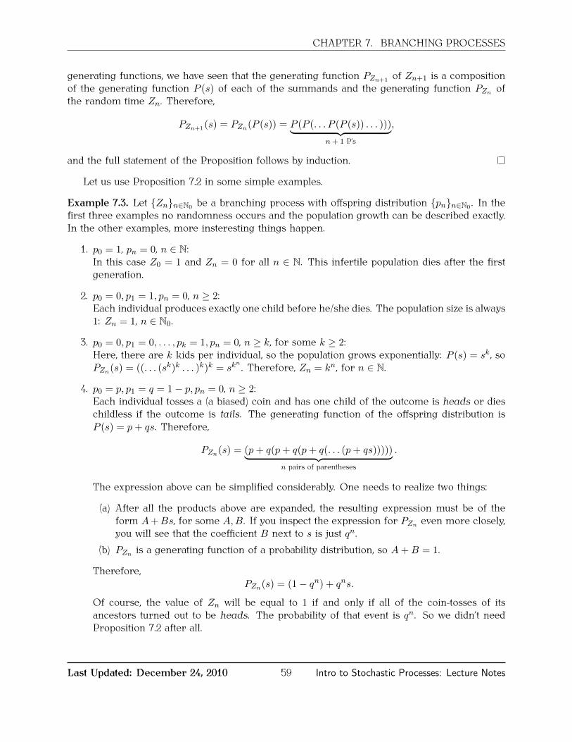
CHAPTER 7. BRANCHING PROCESSES
generating functions, we have seen that the generating function PZn+1 of Zn+1 is a compositionof the generating function P (s) of each of the summands and the generating function PZn ofthe random time Zn. Therefore,
PZn+1(s) = PZn(P (s)) = P (P (. . . P (P (s)) . . . )))︸ ︷︷ ︸n+ 1 P’s
,
and the full statement of the Proposition follows by induction.
Let us use Proposition 7.2 in some simple examples.
Example 7.3. Let Znn∈N0 be a branching process with offspring distribution pnn∈N0 . In thefirst three examples no randomness occurs and the population growth can be described exactly.In the other examples, more insteresting things happen.
1. p0 = 1, pn = 0, n ∈ N:In this case Z0 = 1 and Zn = 0 for all n ∈ N. This infertile population dies after the firstgeneration.
2. p0 = 0, p1 = 1, pn = 0, n ≥ 2:Each individual produces exactly one child before he/she dies. The population size is always1: Zn = 1, n ∈ N0.
3. p0 = 0, p1 = 0, . . . , pk = 1, pn = 0, n ≥ k, for some k ≥ 2:Here, there are k kids per individual, so the population grows exponentially: P (s) = sk , soPZn(s) = ((. . . (sk)k . . . )k)k = sk
n . Therefore, Zn = kn, for n ∈ N.
4. p0 = p, p1 = q = 1− p, pn = 0, n ≥ 2:Each individual tosses a (a biased) coin and has one child of the outcome is heads or dieschildless if the outcome is tails. The generating function of the offspring distribution isP (s) = p+ qs. Therefore,
PZn(s) = (p+ q(p+ q(p+ q(. . . (p+ qs)))))︸ ︷︷ ︸n pairs of parentheses
.
The expression above can be simplified considerably. One needs to realize two things:
(a) After all the products above are expanded, the resulting expression must be of theform A+Bs, for some A,B. If you inspect the expression for PZn even more closely,you will see that the coefficient B next to s is just qn.
(b) PZn is a generating function of a probability distribution, so A+B = 1.
Therefore,PZn(s) = (1− qn) + qns.
Of course, the value of Zn will be equal to 1 if and only if all of the coin-tosses of itsancestors turned out to be heads. The probability of that event is qn. So we didn’t needProposition 7.2 after all.
Last Updated: December 24, 2010 59 Intro to Stochastic Processes: Lecture Notes
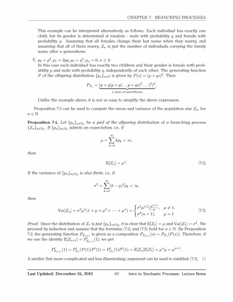
CHAPTER 7. BRANCHING PROCESSES
This example can be interpreted alternatively as follows. Each individual has exactly onechild, but its gender is determined at random - male with probability q and female withprobability p. Assuming that all females change their last name when they marry, andassuming that all of them marry, Zn is just the number of individuals carrying the familyname after n generations.
5. p0 = p2, p1 = 2pq, p2 = q2, pn = 0, n ≥ 3:In this case each individual has exactly two children and their gender is female with prob-ability p and male with probability q, independently of each other. The generating functionP of the offspring distribution pnn∈N is given by P (s) = (p+ qs)2. Then
PZn = (p+ q(p+ q(. . . p+ qs)2 . . . )2)2︸ ︷︷ ︸n pairs of parentheses
.
Unlike the example above, it is not so easy to simplify the above expression.
Proposition 7.2 can be used to compute the mean and variance of the population size Zn, forn ∈ N.
Proposition 7.4. Let pnn∈N0 be a pmf of the offpsring distribution of a branching processZnn∈N0 . If pnn∈N0 admits an expectation, i.e., if
µ =∞∑k=0
kpk <∞,
then
E[Zn] = µn. (7.2)
If the variance of pnn∈N0 is also finite, i.e., if
σ2 =∞∑k=0
(k − µ)2pk <∞,
then
Var[Zn] = σ2µn(1 + µ+ µ2 + · · ·+ µn) =
σ2µn 1−µn+1
1−µ , µ 6= 1,
σ2(n+ 1), µ = 1(7.3)
Proof. Since the distribution of Z1 is just pnn∈N0 , it is clear that E[Z1] = µ and Var[Z1] = σ2. Weproceed by induction and assume that the formulas (7.2) and (7.3) hold for n ∈ N. By Proposition7.2, the generating function PZn+1 is given as a composition PZn+1(s) = PZn(P (s)). Therefore, ifwe use the identity E[Zn+1] = P ′Zn+1
(1), we get
P ′Zn+1(1) = P ′Zn
(P (1))P ′(1) = P ′Zn(1)P ′(1) = E[Zn]E[Z1] = µnµ = µn+1.
A similar (but more complicated and less illuminating) argument can be used to establish (7.3).
Last Updated: December 24, 2010 60 Intro to Stochastic Processes: Lecture Notes

CHAPTER 7. BRANCHING PROCESSES
7.5 Extinction probability
We now turn to the central question (the one posed by Galton). We define extinction to be thefollowing event:
E = ω ∈ Ω : Zn(ω) = 0 for some n ∈ N.
It is the property of the branching process that Zm = 0 for allm ≥ n whenever Zn = 0. Therefore,we can write E as an increasing union of sets En, where
En = ω ∈ Ω : Zn(ω) = 0.
Therefore, the sequence P[En]n∈N is non-decreasing and “continuity of probability” (see thevery first lecture) implies that
P[E] = limn∈N
P[En].
The number P[E] is called the extinction probability. Using generating functions, and, in partic-ular, the fact that P[En] = P[Zn = 0] = PZn(0) we get
P[E] = limn∈N
PZn(0) = limn∈N
P (P (. . . P (0) . . . ))︸ ︷︷ ︸n P’s
.
It is amazing that this probability can be computed, even if the explicit form of the generatingfunction PZn is not known.
Proposition 7.5. The extinction probability p = P[E] is the smallest non-negative solution ofthe equation
x = P (x), called the extinction equation,where P is the generating function of the offspring distribution.
Proof. Let us show first that p = P[E] is a solution of the equation x = P (x). Indeed, P is acontinuous function, so P (limn→∞ xn) = limn→∞ P (xn) for every convergent sequence xnn∈N0
in [0, 1] with xn → x∞. Let us take a particular sequence given by
xn = P (P (. . . P (0) . . . ))︸ ︷︷ ︸n P’s
.
Then
1. p = P[E] = limn∈N xn, and
2. P (xn) = xn+1.
Therefore,p = lim
n→∞xn = lim
n→∞xn+1 = lim
n→∞P (xn) = P ( lim
n→∞xn) = P (p),
and so p solves the equation P (x) = x.The fact that p = P[E] is the smallest solution of x = P (x) on [0, 1] is a bit trickier to get. Let
p′ be another solution of x = P (x) on [0, 1]. Since 0 ≤ p′ and P is a non-decreasiing function, wehave
P (0) ≤ P (p′) = p′.
Last Updated: December 24, 2010 61 Intro to Stochastic Processes: Lecture Notes

CHAPTER 7. BRANCHING PROCESSES
We can apply the function P to both sides of the inequality above to get
P (P (0)) ≤ P (P (p′)) = P (p′) = p′.
Continuing in the same way we get
P [En] = P (P (. . . P (0) . . . ))︸ ︷︷ ︸n P’
≤ p′,
we get p = P[E] = limn∈N P[En] ≤ limn∈N p′ = p′, so p is not larger then any other solution p′ of
x = P (x).
Example 7.6. Let us compute extinction probabilities in the cases from Example 7.3.
1. p0 = 1, pn = 0, n ∈ N:No need to use any theorems. P[E] = 1 in this case.
2. p0 = 0, p1 = 1, pn = 0, n ≥ 2:Like above, the situation is clear - P[E] = 0.
3. p0 = 0, p1 = 0, . . . , pk = 1, pn = 0, n ≥ k, for some k ≥ 2:No extinction here - P[E] = 0.
4. p0 = p, p1 = q = 1− p, pn = 0, n ≥ 2:Since P (s) = p+ qs, the extinction equation is s = p+ qs. If p = 0, the only solution is s = 0,so no extinction occurs. If p > 0, the only solution is s = 1 - the extinction is guaranteed. Itis interesting to note the jump in the extinction probability as p changes from 0 to a positivenumber.
5. p0 = p2, p1 = 2pq, p2 = q2, pn = 0, n ≥ 3:Here P (s) = (p+ qs)2, so the extinction equation reads
s = (p+ qs)2.
This is a quadratic in s and its solutions are s1 = 1 and s2 = p2
q2, if we assume that q > 0.
When p < q, the smaller of the two is s2. When p ≥ q, s = 1 is the smallest solution.Therefore
P[E] = min(1,p2
q2).
Last Updated: December 24, 2010 62 Intro to Stochastic Processes: Lecture Notes

Chapter 8
Markov Chains
8.1 The Markov property
Simply put, a stochastic process has the Markov property if its future evolution depends onlyon its current position, not on how it got there. Here is a more precise, mathematical, definition.It will be assumed throughout this course that any stochastic process Xnn∈N0 takes values ina countable set S - the state space. Usually, S will be either N0 (as in the case of branchingprocesses) or Z (random walks). Sometimes, a more general, but still countable, state space Swill be needed. A generic element of S will be denoted by i or j .
Definition 8.1. A stochastic process Xnn∈N0 talking values in a countable state space S is calleda Markov chain (or said to have the Markov property) if
P[Xn+1 = in+1|Xn = in, Xn−1 = in−1, . . . , X1 = i1, X0 = i0] = P[Xn+1 = in+1|Xn = in], (8.1)
for all n ∈ N0, all i0, i1, . . . , in, in+1 ∈ S , whenever the two conditional probabilities are well-defined, i.e., when P[Xn = in, . . . , X1 = i1, X0 = i0] > 0.
The Markov property is typically checked in the following way: one computes the left-handside of (8.1) and shows that its value does not depend on in−1, in−2, . . . , i1, i0 (why is that enough?).A condition P[Xn = in, . . . , X0 = i0] > 0 will be assumed (without explicit mention) every timewe write a conditional expression like to one in (8.1).
All chains in this course will be homogeneous, i.e., the conditional probabilities P[Xn+1 =j|Xn = i] will not depend on the current time n ∈ N0, i.e., P[Xn+1 = j|Xn = i] = P[Xm+1 =j|Xm = i], for m,n ∈ N0.
Markov chains are (relatively) easy to work with because the Markov property allows usto compute all the probabilities, expectations, etc. we might be interested in by using only twoingredients.
1. Initial probability a(0) = a(0)i : i ∈ S, a(0)i = P[X0 = i] - the initial probability distributionof the process, and
2. Transition probabilities pij = P[Xn+1 = j|Xn = i] - the mechanism that the process usesto jump around.
63

CHAPTER 8. MARKOV CHAINS
Indeed, if one knows all a(0)i and all pij , and wants to compute a joint distribution P[Xn =in, Xn−1 = in−1, . . . , X0 = i0], one needs to use the definition of conditional probability and theMarkov property several times (the multiplication theorem from your elementary probabilitycourse) to get
P[Xn = in, . . . , X0 = i0] = P[Xn = in|Xn−1 = in−1, . . . , X0 = i0]P[Xn−1 = in−1, . . . , X0 = i0]
= P[Xn = in|Xn−1 = in−1]P[Xn−1 = in−1, . . . , X0 = i0]
= pin−1inP[Xn−1 = in−1, . . . , X0 = i0]
Repeating the same procedure, we get
P[Xn = in, . . . , X0 = i0] = pin−1in × pin−2in−1 × · · · × pi0i1 × a(0)i0.
When S is finite, there is no loss of generality in assuming that S = 1, 2, . . . , n, and then weusually organize the entries of a(0) into a row vector
a(0) = (a(0)1 , a
(0)2 , . . . , a(0)n ),
and the transition probabilities pij into a square matrix P, where
P =
p11 p12 . . . p1np21 p22 . . . p2n
...... . . . ...
pn1 pn2 . . . pnn
In the general case (S possibly infinite), one can still use the vector and matrix notation as before,but it becomes quite clumsy in the general case. For example, if S = Z, P is an infinite matrix
P =
. . . ......
... . . .
. . . p−1−1 p−1 0 p−1 1 . . .
. . . p0−1 p0 0 p0 1 . . .
. . . p1−1 p1 0 p1 1 . . .
. . . ......
... . . .
8.2 Examples
Here are some examples of Markov chains - for each one we write down the transition matrix.The initial distribution is sometimes left unspecified because it does not really change anything.
1. Random walks Let Xnn∈N0 be a simple random walk. Let us show that it indeed hasthe Markov property (8.1). Remember, first, that Xn =
∑nk=1 ξk , where ξk are independent
coin-tosses. For a choice of i0, . . . , in+1 (such that i0 = 0 and ik+1 − ik = ±1) we have
P[Xn+1 = in+1|Xn = in, Xn−1 = in−1, . . . , X1 = i1, X0 = i0]
=P[Xn+1 −Xn = in+1 − in|Xn = in, Xn−1 = in−1, . . . , X1 = i1, X0 = i0]
=P[ξn+1 = in+1 − in|Xn = in, Xn−1 = in−1, . . . , X1 = i1, X0 = i0]
=P[ξn+1 = in+1 − in],
Last Updated: December 24, 2010 64 Intro to Stochastic Processes: Lecture Notes

CHAPTER 8. MARKOV CHAINS
where the last equality follows from the fact that the increment ξn+1 is idependent of the previousincrements, and, therefore, of the values of X1, X2, . . . , Xn. The last line above does not dependon in−1, . . . , i1, i0, so X indeed has the Markov property.
The state space S of Xnn∈N0 is the set Z of all integers, and the initial distribution a(0)
is very simple: we start at 0 with probability 1 (so that a(0)0 = 1 and a(0)i = 0, for i 6= 0.). The
transition probabilities are simple to write down
pij =
p, j = i+ 1
q, j = i− 1
0, otherwise.
These can be written down in an infinite matrix,
P =
. . . ......
......
... . . .
. . . 0 P 0 0 0 . . .
. . . q 0 p 0 0 . . .
. . . 0 q 0 p 0 . . .
. . . 0 0 q 0 p . . .
. . . 0 0 0 q 0 . . .
. . . 0 0 0 0 q . . .
. . . ......
......
...... . . .
but it does not help our understanding much.
2. Branching processes Let Xnn∈N0 be a simple Branching process with the branchingdistribution pnn∈N0 . As you surely remember, it is constructed as follows: X0 = 1 and Xn+1 =∑Xn
k=1Xn,k , where Xn,kn∈N0,k∈N is a family of independent random variables with distributionpnn∈N0 . It is now not very difficult to show that Xnn∈N0 is a Markov chain
P[Xn+1 = in+1|Xn = in, Xn−1 = in−1, . . . , X1 = i1, X0 = i0]
=P[
Xn∑k=1
Xn,k = in+1|Xn = in, Xn−1 = in−1, . . . , X1 = i1, X0 = i0]
=P[
in∑k=1
Xn,k = in+1|Xn = in, Xn−1 = in−1, . . . , X1 = i1, X0 = i0]
=P[
in∑k=1
Xn,k = in+1],
where, just like in the random-walk case, the last equality follows from the fact that the randomvariables Xn,k , k ∈ N are independent of all Xm,k , m < n, k ∈ N. In particular, they areindependent of Xn, Xn−1, . . . , X1, X0, which are obtained as combinations of Xm,k , m < n, k ∈ N.The computation above also reveals the structure of the transition probabilities, pij , i, j ∈ S = N0:
pij = P[i∑
k=1
Xn,k = j].
Last Updated: December 24, 2010 65 Intro to Stochastic Processes: Lecture Notes
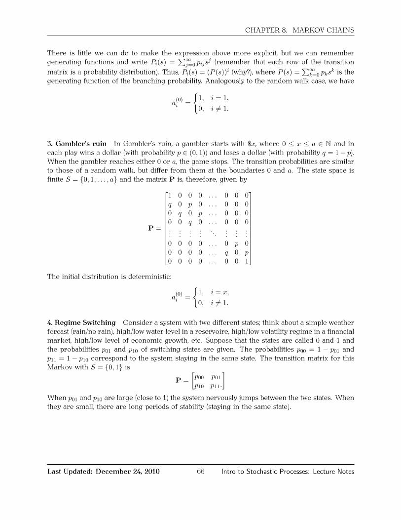
CHAPTER 8. MARKOV CHAINS
There is little we can do to make the expression above more explicit, but we can remembergenerating functions and write Pi(s) =
∑∞j=0 pijs
j (remember that each row of the transitionmatrix is a probability distribution). Thus, Pi(s) = (P (s))i (why?), where P (s) =
∑∞k=0 pks
k is thegenerating function of the branching probability. Analogously to the random walk case, we have
a(0)i =
1, i = 1,
0, i 6= 1.
3. Gambler’s ruin In Gambler’s ruin, a gambler starts with $x, where 0 ≤ x ≤ a ∈ N and ineach play wins a dollar (with probability p ∈ (0, 1)) and loses a dollar (with probability q = 1− p).When the gambler reaches either 0 or a, the game stops. The transition probabilities are similarto those of a random walk, but differ from them at the boundaries 0 and a. The state space isfinite S = 0, 1, . . . , a and the matrix P is, therefore, given by
P =
1 0 0 0 . . . 0 0 0q 0 p 0 . . . 0 0 00 q 0 p . . . 0 0 00 0 q 0 . . . 0 0 0...
......
... . . . ......
...0 0 0 0 . . . 0 p 00 0 0 0 . . . q 0 p0 0 0 0 . . . 0 0 1
The initial distribution is deterministic:
a(0)i =
1, i = x,
0, i 6= 1.
4. Regime Switching Consider a system with two different states; think about a simple weatherforcast (rain/no rain), high/low water level in a reservoire, high/low volatility regime in a financialmarket, high/low level of economic growth, etc. Suppose that the states are called 0 and 1 andthe probabilities p01 and p10 of switching states are given. The probabilities p00 = 1 − p01 andp11 = 1− p10 correspond to the system staying in the same state. The transition matrix for thisMarkov with S = 0, 1 is
P =
[p00 p01p10 p11.
]When p01 and p10 are large (close to 1) the system nervously jumps between the two states. Whenthey are small, there are long periods of stability (staying in the same state).
Last Updated: December 24, 2010 66 Intro to Stochastic Processes: Lecture Notes
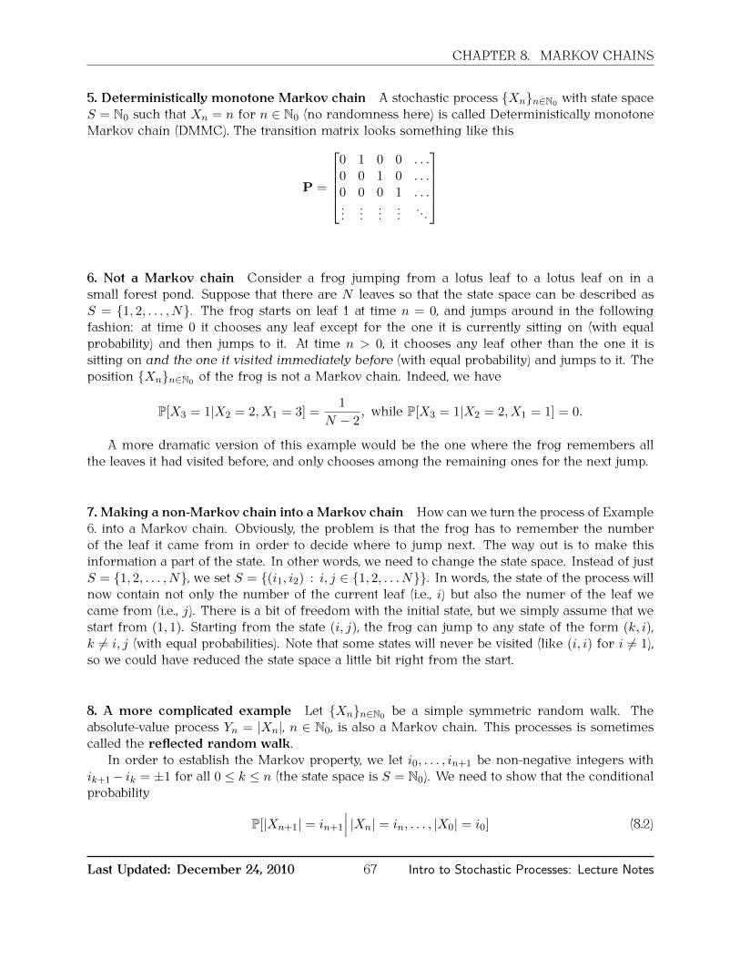
CHAPTER 8. MARKOV CHAINS
5. Deterministically monotone Markov chain A stochastic process Xnn∈N0 with state spaceS = N0 such that Xn = n for n ∈ N0 (no randomness here) is called Deterministically monotoneMarkov chain (DMMC). The transition matrix looks something like this
P =
0 1 0 0 . . .0 0 1 0 . . .0 0 0 1 . . ....
......
... . . .
6. Not a Markov chain Consider a frog jumping from a lotus leaf to a lotus leaf on in asmall forest pond. Suppose that there are N leaves so that the state space can be described asS = 1, 2, . . . , N. The frog starts on leaf 1 at time n = 0, and jumps around in the followingfashion: at time 0 it chooses any leaf except for the one it is currently sitting on (with equalprobability) and then jumps to it. At time n > 0, it chooses any leaf other than the one it issitting on and the one it visited immediately before (with equal probability) and jumps to it. Theposition Xnn∈N0 of the frog is not a Markov chain. Indeed, we have
P[X3 = 1|X2 = 2, X1 = 3] =1
N − 2, while P[X3 = 1|X2 = 2, X1 = 1] = 0.
A more dramatic version of this example would be the one where the frog remembers allthe leaves it had visited before, and only chooses among the remaining ones for the next jump.
7. Making a non-Markov chain into a Markov chain How can we turn the process of Example6. into a Markov chain. Obviously, the problem is that the frog has to remember the numberof the leaf it came from in order to decide where to jump next. The way out is to make thisinformation a part of the state. In other words, we need to change the state space. Instead of justS = 1, 2, . . . , N, we set S = (i1, i2) : i, j ∈ 1, 2, . . . N. In words, the state of the process willnow contain not only the number of the current leaf (i.e., i) but also the numer of the leaf wecame from (i.e., j). There is a bit of freedom with the initial state, but we simply assume that westart from (1, 1). Starting from the state (i, j), the frog can jump to any state of the form (k, i),k 6= i, j (with equal probabilities). Note that some states will never be visited (like (i, i) for i 6= 1),so we could have reduced the state space a little bit right from the start.
8. A more complicated example Let Xnn∈N0 be a simple symmetric random walk. Theabsolute-value process Yn = |Xn|, n ∈ N0, is also a Markov chain. This processes is sometimescalled the reflected random walk.
In order to establish the Markov property, we let i0, . . . , in+1 be non-negative integers withik+1− ik = ±1 for all 0 ≤ k ≤ n (the state space is S = N0). We need to show that the conditionalprobability
P[|Xn+1| = in+1
∣∣∣ |Xn| = in, . . . , |X0| = i0] (8.2)
Last Updated: December 24, 2010 67 Intro to Stochastic Processes: Lecture Notes
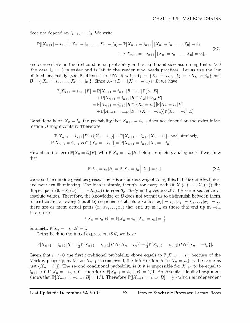
CHAPTER 8. MARKOV CHAINS
does not depend on in−1, . . . , i0. We write
P[|Xn+1| = in+1
∣∣∣ |Xn| = in, . . . , |X0| = i0] = P[Xn+1 = in+1
∣∣∣ |Xn| = in, . . . , |X0| = i0]
+ P[Xn+1 = −in+1
∣∣∣ |Xn| = in, . . . , |X0| = i0],(8.3)
and concentrate on the first conditional probability on the right-hand side, asumming that in > 0(the case in = 0 is easier and is left to the reader who needs practice). Let us use the lawof total probability (see Problem 1 in HW 6) with A1 = Xn = in, A2 = Xn 6= in andB = |Xn| = in, . . . , |X0| = |i0|. Since A2 ∩B = Xn = −in ∩B, we have
P[Xn+1 = in+1|B] = P[Xn+1 = in+1|B ∩A1]P[A1|B]
+ P[Xn+1 = in+1|B ∩A2]P[A2|B]
= P[Xn+1 = in+1|B ∩ Xn = in]P[Xn = in|B]
+ P[Xn+1 = in+1|B ∩ Xn = −in]P[Xn = −in|B]
Conditionally on Xn = in, the probability that Xn+1 = in+1 does not depend on the extra infor-mation B might contain. Therefore
P[Xn+1 = in+1|B ∩ Xn = in] = P[Xn+1 = in+1|Xn = in], and, similarly,P[Xn+1 = in+1|B ∩ Xn = −in] = P[Xn+1 = in+1|Xn = −in].
How about the term P[Xn = in|B] (with P[Xn = −in|B] being completely analogous)? If we showthat
P[Xn = in|B] = P[Xn = in
∣∣∣ |Xn| = in], (8.4)
we would be making great progress. There is a rigorous way of doing this, but it is quite technicaland not very illuminating. The idea is simple, though: for every path (0, X1(ω), . . . , Xn(ω)), theflipped path (0,−X1(ω), . . . ,−Xn(ω)) is equally likely and gives exactly the same sequence ofabsolute values. Therefore, the knowledge of B does not permit us to distinguish between them.In particular, for every (possible) sequence of absolute values |x0| = i0, |x1| = i1, . . . , |x0| = inthere are as many actual paths (x0, x1, . . . , xn) that end up in in as those that end up in −in.Therefore,
P[Xn = in|B] = P[Xn = in
∣∣∣ |Xn| = in] = 12 .
Similarly, P[Xn = −in|B] = 12 .
Going back to the initial expression (8.4), we have
P[Xn+1 = in+1|B] = 12P[Xn+1 = in+1|B ∩ Xn = in] + 1
2P[Xn+1 = in+1|B ∩ Xn = −in].
Given that in > 0, the first conditional probability above equals to P[Xn+1 = in] because of theMarkov property; as far as Xn+1 is concerned, the information B ∩ Xn = in is the same asjust Xn = in). The second conditional probability is 0: it is impossible for Xn+1 to be equal toin+1 > 0 if Xn = −in < 0. Therefore, P[Xn+1 = in+1|B] = 1/4. An essential identical argumentshows that P[Xn+1 = −in+1|B] = 1/4. Therefore P[|Xn+1| = in+1|B] = 1
2 - which is independent
Last Updated: December 24, 2010 68 Intro to Stochastic Processes: Lecture Notes

CHAPTER 8. MARKOV CHAINS
of in−1, . . . , i1, i0 (it looks like it is also independent of in but it is not; this probability is equal to0 unless in+1 − in = ±1).
9. A more realistic example In agame of tennis, the scoring system isas follows: both players (let us callthem Amélie and Björn) start with thescore of 0. Each time Amélie wins apoint, her score moves a step up in thefollowing hierarchy
0 7→ 15 7→ 30 7→ 40.
Once Amélie reaches 40 and scores apoint, three things can happen:
1. if Björn’s score is 30 or less,Amélie wins the game.
2. if Björn’s score is 40, Amélie’sscore moves up to “advantage”,and
3. if Björn’s score is “advantage”,nothing happens to Amélie’sscore, but Björn’s score falls backto 40.
Finally, if Amélie’s score is “advantage”and she wins a point, she wins thegame. The situation is entirely sym-metric for Björn. We suppose that theprobability that Amélie wins each pointis p ∈ (0, 1), independently of the cur-rent score.
q
p
q
p
q
p
q
q
q
p
p
q
q
p
p
q
p
q
1
q
p
q
p
q
p
p
q
q
p
p
q
p
q
1
p
q
p
q
80, 0<
80, 15<
815, 0<
80, 30<
815, 15<
80, 40<
815, 30<
815, 40<
830, 40<
Bjorn wins
830, 0<
830, 15<
830, 30<
840, 0<
840, 15<
840, 30<
840, 40<
Amelie wins
8Adv, 40<
840, Adv<
Figure. Markov chains with a finite number of states areusually represented by directed graphs (like the one inthe figure above). The nodes are states, two states i, j arelinked by a (directed) edge if the transition probability pijis non-zero, and the number pij is writen above the link.If pij = 0, no edge is drawn.
A situation like this is a typical example of a Markov chain in an applied setting. What arethe states of the process? We obviously need to know both players’ scores and we also need toknow if one of the players has won the game. Therefore, a possible state space is the following:
S =
“Amelie wins”, “Bjorn wins”, (0, 0), (0, 15), (0, 30), (0, 40), (15, 0), (15, 15), (15, 30), (15, 40),
(30, 0), (30, 15), (30, 30), (30, 40), (40, 0), (40, 15), (40, 30), (40, 40), (40,Adv), (Adv, 40)
(8.5)
It is not hard to assign probabilities to transitions between states. Once we reach either “Ameliewins” or “Bjorn wins” the game stops. We can assume that the chain remains in that state forever,i.e., the state is absorbing. The initial distribution is quite simple - we aways start from the samestate (0, 0), so that a(0)(0,0) = 1 and a(0)i = 0 for all i ∈ S \ 0.
Last Updated: December 24, 2010 69 Intro to Stochastic Processes: Lecture Notes

CHAPTER 8. MARKOV CHAINS
How about the transition matrix? When the number of states is big (#S = 20 in this case),transition matrices are useful in computer memory, but not so much on paper. Just for the funof it, here is the transition matrix for our game-of-tennis chain, with the states ordered as in (8.5):
P =
1 0 0 0 0 0 0 0 0 0 0 0 0 0 0 0 0 0 0 00 1 0 0 0 0 0 0 0 0 0 0 0 0 0 0 0 0 0 00 0 0 q 0 0 p 0 0 0 0 0 0 0 0 0 0 0 0 00 0 0 0 q 0 0 p 0 0 0 0 0 0 0 0 0 0 0 00 0 0 0 0 q 0 0 p 0 0 0 0 0 0 0 0 0 0 00 q 0 0 0 0 0 0 0 p 0 0 0 0 0 0 0 0 0 00 0 0 0 0 0 0 q 0 0 p 0 0 0 0 0 0 0 0 00 0 0 0 0 0 0 0 q 0 0 p 0 0 0 0 0 0 0 00 0 0 0 0 0 0 0 0 q 0 0 p 0 0 0 0 0 0 00 q 0 0 0 0 0 0 0 0 0 0 0 p 0 0 0 0 0 00 0 0 0 0 0 0 0 0 0 0 q 0 0 p 0 0 0 0 00 0 0 0 0 0 0 0 0 0 0 0 q 0 0 p 0 0 0 00 0 0 0 0 0 0 0 0 0 0 0 0 q 0 0 p 0 0 00 q 0 0 0 0 0 0 0 0 0 0 0 0 0 0 0 p 0 0p 0 0 0 0 0 0 0 0 0 0 0 0 0 0 q 0 0 0 0p 0 0 0 0 0 0 0 0 0 0 0 0 0 0 0 q 0 0 0p 0 0 0 0 0 0 0 0 0 0 0 0 0 0 0 0 q 0 00 0 0 0 0 0 0 0 0 0 0 0 0 0 0 0 0 0 q p0 q 0 0 0 0 0 0 0 0 0 0 0 0 0 0 0 p 0 0p 0 0 0 0 0 0 0 0 0 0 0 0 0 0 0 0 q 0 0
Here is a question we will learn how to answer later:
Question 8.2. Does the structure of a game of tennis make is easier or harder for the betterplayer to win? In other words, if you had to play against Roger Federer (I am rudely assumingthat he is better than you), would you have a better chance of winning if you only played a point,or if you actually played the whole game?
8.3 Chapman-Kolmogorov relations
The transition probabilities pij , i, j ∈ S tell us how a Markov chain jumps from a state to astate in one step. How about several steps, i.e., how does one compute the the probabilities likeP[Xk+n = j|Xk = i], n ∈ N? Since we are assuming that all of our chains are homogeneous(transition probabilities do not change with time), this probability does not depend on the time k,and we set
p(n)ij = P[Xk+n = j|Xk = i] = P[Xn = j|X0 = i].
It is sometimes useful to have a more compact notation for this, last, conditional probability, sowe write
Pi[A] = P[A|X0 = i], for any event A.
Therefore,p(n)ij = Pi[Xn = j].
Last Updated: December 24, 2010 70 Intro to Stochastic Processes: Lecture Notes

CHAPTER 8. MARKOV CHAINS
For n = 0, we clearly have
p(0)ij =
1, i = j,
0, i 6= j.
Once se have defined the multi-step transition probabilities p(n)ij , i, j ∈ S , n ∈ N0, we need to
be able to compute them. This computation is central in various applications of Markov chains:they relate the small-time (one-step) behavior which is usually easy to observe and model to along-time (multi-step) behavior which is really of interest. Before we state the main result in thisdirection, let us remember how matrices are multiplied. When A and B are n× n matrices, theproduct C = AB is also an n× n matrix and its ij-entry Cij is given as
Cij =n∑k=1
AikBkj .
There is nothing special about finiteness in the above definition. If A and B were infinite matricesA = (Aij)i,j∈S , B = (Bij)i,j∈S for some countable set S , the same procedure could be used todefine C = AB. Indeed, C will also be an “S × S ”-matrix and
Cij =∑k∈S
AikBkj ,
as long as the (infinite) sum above converges absolutely. In the case of a typical transition matrixP, convergence will not be a problem since P is a stochastic matrix, i.e., it has the following twoproperties (why?):
1. pij ≥ 0, for all i, j ∈ S , and
2.∑
j∈S pij = 1, for all i ∈ S (in particular, pij ∈ [0, 1], for all i, j).
When P = (pij)i,j∈S and P′ = (p′ij)i,j∈S are two S×S-stochastic matrices, the series∑
k∈S pikp′kj
converges absolutely since 0 ≤ p′kj ≤ 1 for all k, j ∈ S and so∑k∈S
∣∣pikp′kj∣∣ ≤∑k∈S
pik ≤ 1, for all i, j ∈ S.
Moreover, a product C of two stochastic matrices A and B is always a stochastic matrix: theentries of C are clearly positive and (by Tonelli’s theorem)∑
j∈SCij =
∑j∈S
∑k∈S
AikBkj =∑k∈S
∑j∈S
AikBkj =∑k∈S
Aik∑j∈S
Bkj︸ ︷︷ ︸1
=∑k∈S
Aik = 1.
Proposition 8.3. Let Pn be the n-th (matrix) power of the transition matrix P. Then p(n)ij =
(Pn)ij , for i, j ∈ S .
Last Updated: December 24, 2010 71 Intro to Stochastic Processes: Lecture Notes

CHAPTER 8. MARKOV CHAINS
Proof. We proceed by induction. For n = 1 the statement follows directly from the definition ofthe matrix P. Supposing that p(n)ij = (Pn)ij for all i, j , we have
p(n+1)ij = P[Xn+1 = j|X0 = i]
=∑k∈S
P[X1 = k|X0 = i]P[Xn+1 = j|X0 = i,X1 = k]
=∑k∈S
P[X1 = k|X0 = i]P[Xn+1 = j|X1 = k]
=∑k∈S
P[X1 = k|X0 = i]P[Xn = j|X0 = k]
=∑k∈S
pikp(n)kj .
where the second equality follows from the law of total probability, the third one from the Markovproperty, and the fourth one from homogeneity. The last sum above is nothing but the expressionfor the matrix product of P and Pn, and so we have proven the induction step.
Using Proposition 8.3, we can write a simple expression for the distribution of the randomvariable Xn, for n ∈ N0. Remember that the initial dsitribution (the distribution of X0) is denotedby a(0) = (a
(0)i )i∈S . Analogously, we define the vector a(n) = (a
(n)i )i∈S by
a(n)i = P[Xn = i], i ∈ S.
Using the law of total probability, we have
a(n)i = P[Xn = i] =
∑k∈S
P[X0 = k]P[Xn = i|X0 = k] =∑k∈S
a(0)k p
(n)ki .
We usually interpret a(0) as a (row) vector, so the above relationship can be expressed usingvector-matrix multiplication
a(n) = a(0)Pn.
The following corollary shows a simple, yet fundamental, relationship between different multi-step transition probabilities p(n)ij .
Corollary 8.4 (Chapman-Kolmogorov relations). For n,m ∈ N0 and i, j ∈ S we have
p(m+n)ij =
∑k∈S
p(m)ik p
(n)kj .
Proof. The statement follows directly from the matrix equality
Pm+n = PmPn.
Last Updated: December 24, 2010 72 Intro to Stochastic Processes: Lecture Notes

CHAPTER 8. MARKOV CHAINS
It is usually difficult to compute Pn for a general transition matrix P and a large n. We willsee later that it will be easier to find the limiting values limn→∞ p
(n)ij . In the mean-time, here is a
simple example where this can be done by hand
Example 8.5. In the setting of a Regime Switching chain (Example 4.), let us write a for p01 andb for p10 to simplify the notation, so that the transition matrix looks like this:
P =
[1− a ab 1− b
]The characteristic equation det(λI −P) = 0 of the matrix P is
0 = det(λI −P) =
∣∣∣∣λ− 1 + a −a−b λ− 1 + b
∣∣∣∣ = ((λ− 1) + a)((λ− 1) + b)− ab
= (λ− 1)(λ− (1− a− b)).
The eigenvalues are, therefore, λ1 = 1 and λ2 = 1 − a − b. The eigenvectors are v1 =(11
)and
v2 =(a−b), so that with V =
[1 a1 −b
]and D =
[λ1 00 λ2
]=
[1 00 (1− a− b)
]we have
PV = V D, i.e., P = V DV −1.
This representation is very useful for taking matrix powers:
Pn = (V DV −1)(V DV −1) . . . (V DV −1) = V DnV −1 = V
[1 00 (1− a− b)n
]V −1
Assuming a+ b > 0 (i.e., P 6=[0 11 0
]), we have V −1 = 1
a+b
[b a1 −1
], and
Pn = V DnV −1 =
[1 a1 −b
] [1 00 (1− a− b)n
]1a+b
[b a1 −1
]=
1
a+ b
[b ab a
]+
(1− a− b)n
a+ b
[a −ab −b
]
=
ba+b + (1− a− b)n a
a+baa+b − (1− a− b)n a
a+b
ba+b + (1− a− b)n b
a+baa+b − (1− a− b)n b
a+b
The expression for Pn above tells us a lot about the structure of the multi-step probabilities
p(n)ij for large n. Note that the second matrix on the right-hand side above comes multiplied by
(1− a− b)n which tends to 0 as n→∞, unless we are in the uninteresting situation a = b = 0 or(a = b = 1). Therefore,
Pn ∼ 1
a+ b
[a ba b
]for large n.
The fact that the rows of the right-hand side above are equal points to the fact that, for large n,p(n)ij does not depend (much) on the initial state i. In other words, this Markov chain forgets its
initial condition after a long period of time. This is a rule more than an exception, and we willstudy such phenomena in the following lectures.
Last Updated: December 24, 2010 73 Intro to Stochastic Processes: Lecture Notes

Chapter 9
The “Stochastics” package
Stochastics is a Mathematica package (a collection of functions) for various calculations, sim-ulation and visualization of Markov chains. Here is a short user’s guide.
9.1 Installation
You can download the file Stochastics.m from the course web-site. It needs to be put in adirectory/folder on your system that Mathematica knows about. The easiest way to do this isto type $Path in Mathematica. The output will be a list of folders. You simply copy the fileStochastics.m in any of the folders listed. Restart Mathematica, and that is it.
Every time you want to use functions from Stochastics, you issue the command <<Stochastics‘(note that the last symbol ‘ is not an apostrophe; it can be found above the Tab key on your key-board).
If you want to get information about the syntax and usage of a certain command (sayBuildChain), just type ?BuildChain, and Mathematica will display a short help paragraph.
9.2 Building Chains
The first thing you need to learn is to tell Mathematica about the structure of the Markov Chainyou want to analyze. As you know, two ingredients are needed for that: the initial distribution, andthe set of transition probabilities. Since the transition matrix is usually quite sparse (has manyzero elements), it is typically faster to specify those probabilities as a list of transitions of theform FromState,ToState,probability. That is exactly how Stochastics is set up. In order tostore the information about a Markov Chain that Mathematica can do further computations with,you issue the command MyChain=BuildChain[Triplets,InitialDistrubution], where MyChainis just the name of the variable (could be anything), Triplets is a list each of whose elements isa triplet of the from FromState,ToState,probability, and InitialDistribution is a list ofpairs of the form State,probability where probability= P[X0 =State]. Here is an examplefor the simple Markov chain with three states A,B and C, the initial distribution P[X0 = A] = 1/2,P[X0 = B] = 1/4 and P[X0 = C] = 1/4, and the transition graph that looks like this:
74

CHAPTER 9. THE “STOCHASTICS” PACKAGE
0.5 0.5 1.00.5 0.5A B C
The code I used to define it isIn[1]:= << Stochastics`
In[34]:= MyChain = BuildChain @
88A, B, 1 2<, 8A, A, 1 2<, 8B, C, 1 <, 8C, C, 1 2<, 8C, B, 1 2<<,
88A, 1 2<, 8B, 1 4<, 8C, 1 4<<
D;
The “Tennis Chain” example we covered in class is already implemented in the package, so thatyou don’t have to type it in yourself. All you need to do it issue the command MyChain=TennisChain[p],where p is the probability of winning a rally for Amélie.
9.3 Getting information about a chain
Once you have built a chain (assume that its name is MyChain) you can get information about itusing the following commands. We start by listing the simple ones:
• States[MyChain] returns the list of all states.
• InitialDistribution[MyChain] returns the list containing the list of initial probabilities.The order is the same as that returned by the command States.
• TransitionMatrix[MyChain] returns the transition matrix.
• Probability[s1,s2,n,MyChain] returns the n-step probability P[Xn = s2|X0 = s1].
• NumberOfStates[MyChain] returns the number of states.
• Classes[MyChain] returns a list whose elements are the communication classes (lists them-selves) of the chain.
• Recurrence[MyChain] returns a list of zeros or ones, one for each state. It is 1 if the stateis recurrent and 0 otherwise.
• TransientStates[MyChain] returns the list of transient states.
• RecurrentStates[MyChain] returns the list of recurrent states.
• ClassNumber[s,MyChain] returns the number of the communication class the state s be-longs to, i.e., the number of the element of Classes[MyChain] that s belongs to.
See Example 1 for a Mathematica notebook which illustrates these commands using MyChaindefined above. The following commands help with more complicated (matrix) computations:
• QMatrix[MyChain], RMatrix[MyChain] and PMatrix[MyChain] return the matrices Q, R andP from the canonical decomposition of MyChain.
Last Updated: December 24, 2010 75 Intro to Stochastic Processes: Lecture Notes

CHAPTER 9. THE “STOCHASTICS” PACKAGE
• CanonicalForm[MyChain] returns the 2x2 block matrix representation of the canonical formof the chain MyChain
• FundamentalMatrix[MyChain] returns the fundamental matrix (I −Q)−1 of the chain.
See Example 9.2 for a related Mathematica notebook.
9.4 Simulation
The functions in Stochastics can be used to perform repeated simulations of Markov chains:
• SimulateFirst[MyChain] outputs a single draw from the initial distribution of the chain.
• SimulateNext[s,MyChain] outputs a single draw from tomorrow’s position of the chain ifit is in the state s today.
• SimulatePaths[nsim,nsteps,MyChain] outputs a matrix with nsim rows and nsteps columns;each row is a simulated path of the chain of length nsteps.
See Example 9.3 for an illustration.
9.5 Plots
Finally, the package Stochastics can produce pretty pictures and animations of your chains:
• PlotChain[MyChain,Options] produces a graphical representation of the Markov ChainMyChain. The Options argument is optional and can be used to change the look and feelof the plot. Any option that the built-in function GraphPlot accepts can be used.
• AnimateChain[nsteps,Mychain] produces an animation of a single simulated trajectory ofMyChain.
The picture in section 9.2 is the output of the command PlotChain[MyChain].
Last Updated: December 24, 2010 76 Intro to Stochastic Processes: Lecture Notes

CHAPTER 9. THE “STOCHASTICS” PACKAGE
9.6 Examples
Example 9.1. Simple commands
In[1]:= << Stochastics`
In[2]:= MyChain = BuildChain @
88A, B, 1 2<, 8A, A, 1 2<, 8B, C, 1 <, 8C, C, 1 2<, 8C, B, 1 2<<,
88A, 1 2<, 8B, 1 4<, 8C, 1 4<<
D;
In[3]:= States @MyChain D
Out[3]= 8A, B, C<
In[4]:= NumberOfStates @MyChain D
Out[4]= 3
In[6]:= InitialDistribution @MyChain D
Out[6]= :1
2,1
4,1
4>
In[7]:= TransitionMatrix @MyChain D
Out[7]= ::1
2,1
2, 0>, 80, 0, 1<, :0,
1
2,1
2>>
In[8]:= MatrixForm @TransitionMatrix @MyChain DD
Out[8]//MatrixForm=1
2
1
20
0 0 1
0 1
2
1
2
In[9]:= Probability @A, B, 3, MyChain D
Out[9]=3
8
In[10]:= Classes @MyChain D
Out[10]= 88A<, 8B, C<<
In[11]:= Recurrence @MyChain D
Out[11]= 80, 1, 1<
In[12]:= TransientStates @MyChain D
Out[12]= 8A<
In[13]:= RecurrentStates @MyChain D
Out[13]= 8B, C<
Example 9.2. Canonical-form related commands (a continuation of Example 9.1)
Last Updated: December 24, 2010 77 Intro to Stochastic Processes: Lecture Notes

CHAPTER 9. THE “STOCHASTICS” PACKAGE
In[14]:= QMatrix@MyChainD
Out[14]= ::1
2>>
In[15]:= RMatrix@MyChainD
Out[15]= ::1
2, 0>>
In[16]:= PMatrix@MyChainD
Out[16]= :80, 1<, :1
2,1
2>>
In[19]:= M = CanonicalForm@MyChainD
Out[19]= :::80, 1<, :1
2,1
2>>, 880<, 80<<>, :::
1
2, 0>>, ::
1
2>>>>
In[20]:= MatrixForm@
8
8MatrixForm@M@@1, 1DDD, MatrixForm@M@@1, 2DDD<,
8MatrixForm@M@@2, 1DDD, MatrixForm@M@@2, 2DDD<
<
D
Out[20]//MatrixForm=
0 11
2
1
2
0
0
I 1
20 M I 1
2M
In[21]:= FundamentalMatrix@MyChainD
Out[21]= 882<<
Example 9.3. Simulations (a continuation of Example 9.1)
In[22]:= SimulateFirst@MyChainD
Out[22]= A
In[23]:= SimulateFirst@MyChainD
Out[23]= C
In[24]:= SimulateNext@A, MyChainD
Out[24]= A
In[28]:= SimulateNext@A, MyChainD
Out[28]= B
In[36]:= MatrixForm@SimulatePaths@3, 10, MyChainDD
Out[36]//MatrixForm=
C B C B C C B C B C
A A B C C B C B C B
A A A B C B C C B C
Last Updated: December 24, 2010 78 Intro to Stochastic Processes: Lecture Notes
Chapter 10
Classification of States
There will be a lot of definitions and some theory before we get to examples. You might want topeek into the last part (examples) as notions are being introduced; it will help your understanding.
10.1 The Communication Relation
Let Xnn∈N0 be a Markov chain on the state space S . For a given set B of states, define thehitting time τ(B) of B as
τB = minn ∈ N0 : Xn ∈ B. (10.1)
We know that τB is, in fact, a stopping time with respect to Xnn∈N0 . When B consists of onlyone element B = i, we simply write τi for τi; τi is the first time the Markov chain Xnn∈N0
“hits” the state i. As always, we allow τB to take the value +∞; it means that no state in B is everhit.
The hitting times are important both for immediate applications of Xnn∈N0 , as well as forbetter understanding of the structure of Markov chains.
Example 10.1. Let Xnn∈N0 be the chain which models a game of tennis (Example 9., in Section2. of Lecture 8). The probability of winning for (say) Amélie can be phrased in terms of hittingtimes:
P[ Amélie wins ] = P[τiA < τiB ],
where iA = “Amélie wins” and iB =“Björn wins” (the two absorbing states of the chain). We willlearn how to compute such probabilities in the subsequent lectures.
Having introduced the hitting times τB , let us give a few more definitions. Recall that thenotation Pi[A] is used to mean P[A|X0 = i] (for any event A). In practice, we use Pi to signify thatwe are starting the chain from the state i, i.e., Pi corresponds to a Markov chain whose transitionmatrix is the same as the one of Xnn∈N0 , but the initial distribution is given by Pi[X0 = j] = 0if j 6= i and Pi[X0 = i] = 1.
Definition 10.2. A state i ∈ S is said to communicate with the state j ∈ S , denoted by i→ j if
Pi[τj <∞] > 0.
79

CHAPTER 10. CLASSIFICATION OF STATES
Intuitively, i communicates with j is there is a non-zero chance that the Markov chain X willeventually visit j if it starts from i. Sometimes we also say that j is a consequent of i, or that jis accessible from i.
Example 10.3. In the tennis example, every state is accessible from (0, 0) (the fact that p ∈ (0, 1)is important here), but (0, 0) is not accessible from any other state. The consequents of (40, 40)are (40, 40) itself, (40, Adv), (Adv, 40), “Amélie wins” and “Björn wins”.
Before we examine some properties of the relation →, here is a simple but useful charac-terization. Before we give it, we recall the following fact about probability: let Ann∈N0 be anincreasing sequence of events, i.e., An ⊆ An+1, for all n ∈ N0. Then
P[∪n∈N0An] = limn
P[An],
and the sequence inside the limit is non-decreasing.
Proposition 10.4. i→ j if and only if p(n)ij > 0 for some n ∈ N0.
Proof. The event A = τj <∞ can be written as an increasing union
A = ∪n∈NAn, where An = τj ≤ n.
Therefore,Pi[τj <∞] = Pi[A] = lim
nPi[An] = lim
nPi[τj ≤ n],
and the sequence Pi[τj ≤ n], n ∈ N is non-decreasing. In particular,
Pi[τj <∞] ≥ Pi[An], for all n ∈ N. (10.2)
Suppose, first, that p(n)ij > 0 for some n. Since τj is the first time j is visited, we have
Pi[An] = Pi[τj ≤ n] ≥ Pi[Xj = n] = p(n)ij > 0.
By (10.2), we have Pi[τj <∞] > 0, and so, i→ j .Conversely, suppose that i → j , i.e., Pi[A] > 0. Since Pi[A] = limn Pi[An], we must have
Pi[An] > 0 for some n0 (and then all larger n), i.e., Pi[τj ≤ n0] > 0. When τj ≤ n0, we must haveX0 = j or X1 = j or . . . or Xn = j , i.e.,
τj ≤ n0 ⊆ ∪n0k=0Xk = j,
and so
0 < Pi[τj ≤ n0] ≤ Pi[∪n0k=0Xk = j] ≤
n0∑k=0
Pi[Xk = j].
Therefore, Pi[Xn = j] for at least one n ∈ 0, 1, . . . , n0. In other words, p(n)ij > 0, for at least onen ∈ 0, 1, . . . , n0.
Proposition 10.5. For all i, j, k ∈ S , we have
Last Updated: December 24, 2010 80 Intro to Stochastic Processes: Lecture Notes
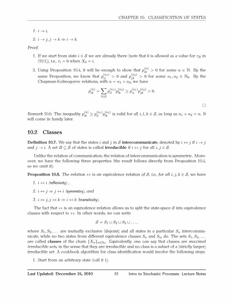
CHAPTER 10. CLASSIFICATION OF STATES
1. i→ i,
2. i→ j, j → k ⇒ i→ k.
Proof.
1. If we start from state i ∈ S we are already there (note that 0 is allowed as a value for τB in(10.1)), i.e., τi = 0 when X0 = i.
2. Using Proposition 10.4, it will be enough to show that p(n)ik > 0 for some n ∈ N. By thesame Proposition, we know that p(n1)
ij > 0 and p(n2)jk > 0 for some n1, n2 ∈ N0. By the
Chapman-Kolmogorov relations, with n = n1 + n2, we have
p(n)ik =
∑l∈S
p(n1)il p
(n2)lk ≥ p(n1)
ij p(n2)jk > 0.
Remark 10.6. The inequality p(n)ik ≥ p(n1)il p
(n2)lk is valid for all i, l, k ∈ S , as long as n1 + n2 = n. It
will come in handy later.
10.2 Classes
Definition 10.7. We say that the states i and j in S intercommunicate, denoted by i↔ j if i→ jand j → i. A set B ⊆ S of states is called irreducible if i↔ j for all i, j ∈ S .
Unlike the relation of communication, the relation of intercommunication is symmetric. More-over, we have the following three properties (the result follows directly from Proposition 10.4,so we omit it):
Proposition 10.8. The relation ↔ is an equivalence relation of S , i.e., for all i, j, k ∈ S , we have
1. i↔ i (reflexivity) ,
2. i↔ j ⇒ j ↔ i (symmetry), and
3. i↔ j, j ↔ k ⇒ i↔ k (transitivity).
The fact that ↔ is an equivalence relation allows us to split the state-space S into equivalenceclasses with respect to ↔. In other words, we can write
S = S1 ∪ S2 ∪ S3 ∪ . . . ,
where S1, S2, . . . are mutually exclusive (disjoint) and all states in a particular Sn intercommu-nicate, while no two states from different equivalence classes Sn and Sm do. The sets S1, S2, . . .are called classes of the chain Xnn∈N0 . Equivalently, one can say that classes are maximalirreducible sets, in the sense that they are irreducible and no class is a subset of a (strictly larger)irreducible set. A cookbook algorithm for class identification would involve the following steps:
1. Start from an arbitrary state (call it 1).
Last Updated: December 24, 2010 81 Intro to Stochastic Processes: Lecture Notes

CHAPTER 10. CLASSIFICATION OF STATES
2. Identify all states j that communicate with it - don’t forget that always i↔ i, for all i.
3. That is your first class, call it C1. If there are no elements left, then there is only one classC1 = S . If there is an element in S \ C1, repeat the procedure above starting from thatelement.
The notion of a class is especially useful in relation to another natural concept:
Definition 10.9. A set B ⊆ S of states is said to be closed if i 6→ j for all i ∈ B and all j ∈ S \B.A state i ∈ S such that the set i is closed is called absorbing.
Here is a nice characterization of closed sets:
Proposition 10.10. A set B of states is closed if and only if pij = 0 for all i ∈ B and allj ∈ Bc = S \B.
Proof. Suppose, first, that B is closed. Then for i ∈ B and j ∈ Bc, we have i 6→ j , i.e., p(n)ij = 0 forall n ∈ N. In particular, pij = 0.
Conversely, suppose that pij = 0 for all i ∈ B, j ∈ Bc. We need to show that i 6→ j (i.e. p(n)ij = 0for all n ∈ N) for all i ∈ B, j ∈ Bc. Suppose, to the contrary, that there exist i ∈ B and j ∈ Bc
such that p(n)ij > 0 for some n ∈ N. Since pij = 0, we must have n > 1. Out of all n > 1 such thatp(n)ik > 0 for some k ∈ Bc, we pick the smallest one (let us call it n0), so that that p(n0−1)
ik = 0 forall k ∈ Bc. By the Chapman-Kolmogorov relation, we have
p(n)ij =
∑k∈S
p(n−1)ik pkj
=∑k∈B
p(n−1)ik pkj +
∑k∈Bc
p(n−1)ik pkj .
(10.3)
The terms in the first sum in the second line of (10.3) are all zero because pkj = 0 (k ∈ B andj ∈ Bc), and the terms of the second one are also all zero because p
(n−1)ik = 0 for all k ∈ Bc.
Therefore, p(n)ij = 0 - a contradiction.
Intuitively, a set of states is closed if it has the property that the chain Xnn∈N0 stays in itforever, once it enters it. In general, if B is closed, it does not have to follow that S \B is closed.Also, a class does not have to be closed, and a closed set does not have to be a class. Here aresome examples:
Example 10.11. Consider the tennis chain of the previous lecture and consider the followingthree sets of states:
1. B = “Amélie wins”: closed and a class, but S \B is not closed
2. B = S \ (0, 0): closed, but not a class, and
3. B = (0, 0): class, but not closed.
There is a relationship between classes and the notion of closedness:
Last Updated: December 24, 2010 82 Intro to Stochastic Processes: Lecture Notes

CHAPTER 10. CLASSIFICATION OF STATES
Proposition 10.12. Every closed set B is a union of classes.
Proof. Let B be the union of all classes C such that C ∩ B 6= ∅. In other words, take all theelements of B and throw in all the states which intercommunicate with them. I claim thatB = B. Blearly, B ⊂ B, so we need to show that B ⊆ B. Suppose, to the contrary, that thereexists j ∈ B \ B. By construction, j intercommunicates with some i ∈ B. In particular i → j .By closedness of B, we must have j ∈ B. This is a contradiction with the assumptions thatj ∈ B \B.
Example 10.13. A converse of Proposition 10.12 is not true. Just take the set B = (0, 0), (0, 15)in the “tennis” example. It is a union of classes, but it is not closed.
10.3 Transience and recurrence
It is often important to know whether a Markov chain will ever return to its initial state, and ifso, how often. The notions of transience and recurrence address this questions.
Definition 10.14. The (first) visit time to state j , denoted by τj(1) is defined as
τj(1) = minn ∈ N : Xn = j.
As usual τj(1) = +∞ if Xn 6= j for all n ∈ N.
Note that the definition of the random variable τj(1) differs from the definition of τj in thatthe minimum here is take over the set N of natural numbers, while the set of non-negativeintegers N0 is used for τj . When X0 6= j , the hitting time τj and the visit time τj(1) coincide.The important difference occurs when X0 = j . In that case τj = 0 (we are already there), but itis always true that τj(1) ≥ 1. It can even happen that Pi[τi(1) =∞] = 1.
Definition 10.15. A state i ∈ S is said to be
1. recurrent if Pi[τi(1) <∞] = 1,
2. positive recurrent if Ei[τi(1)] <∞ (Ei means expectation when the probability is Pi),
3. null recurrent if it is recurrent, but not positive recurrent,
4. transient if it is not recurrent.
A state is recurrent if we are sure we will come back to it eventually (with probability 1).It is positive recurrent if the time between two consecutive visits has finite expectation. Nullrecurrence means the we will return, but the waiting time may be very long. A state is transientis there is a positive chance (however small) that the chain will never return to it.
Remember that the greatest common denominator (GCD) of a set A of natural numbersif the largest number d such that d divides each k ∈ A, i.e., such that each k ∈ A is of the formk = ld for some l ∈ N.
Definition 10.16. A period d(i) of a state i ∈ S is the greatest common denominator of thereturn-time set R(i) = n ∈ N : p
(n)ii > 0 of the state i. When R(i) = ∅, we set d(i) = 1. A state
i ∈ S is called aperiodic if d(i) = 1.
Last Updated: December 24, 2010 83 Intro to Stochastic Processes: Lecture Notes

CHAPTER 10. CLASSIFICATION OF STATES
Example 10.17. Consider the Markov chain with three states and the transition matrix
P =
0 1 00 0 11 0 0
.The return set for each state i ∈ 1, 2, 3 is given by
R(i) = 3, 6, 9, 12, . . . ,
so d(i) = 3 for all i ∈ 1, 2, 3. However, if we change the probabilities a bit:
P =
0 1 00 0 112 0 1
2
,the situation changes drastically:
R(1) = 3, 4, 5, 6, . . . ,R(2) = 2, 3, 4, 5, 6, . . . ,R(3) = 1, 2, 3, 4, 5, 6, . . . ,
so that d(i) = 1 for i ∈ 1, 2, 3.
10.4 Examples
Random walks: p ∈ (0, 1).• Communication and classes. Clearly, it is possible to go from any state i to either i+ 1 ori− 1 in one step, so i→ i+ 1 and i→ i− 1 for all i ∈ S . By transitivity of communication,we have i → i + 1 → i + 2 → · · · → i + k. Similarly, i → i − k for any k ∈ N. Therefore,i→ j for all i, j ∈ S , and so, i↔ j for all i, j ∈ S , and the whole S is one big class.
• Closed sets. The only closed set is S itself.
• Transience and recurrence We studied transience and recurrence in the lectures aboutrandom walks (we just did not call them that). The situation highly depends on the proba-bility p of making an up-step. If p > 1
2 , there is a positive probability that the first step willbe “up”, so that X1 = 1. Then, we know that there is a positive probability that the walk willnever hit 0 again. Therefore, there is a positive probability of never returning to 0, whichmeans that the state 0 is transient. A similar argument can be made for any state i and anyprobability p 6= 1
2 . What happens when p = 12? In order to come back to 0, the walk needs
to return there from its position at time n = 1. If it went up, the we have to wait for thewalk to hit 0 starting from 1. We have shown that this will happen sooner or later, but thatthe expected time it takes is infinite. The same argument works if X1 = −1. All in all, 0(and all other states) are null-recurrent (recurrent, but not positive recurrent).
• Periodicity. Starting from any state i ∈ S , we can return to it after 2, 4, 6, . . . steps. There-fore, the return set R(i) is always given by R(i) = 2, 4, 6, . . . and so d(i) = 2 for alli ∈ S .
Last Updated: December 24, 2010 84 Intro to Stochastic Processes: Lecture Notes

CHAPTER 10. CLASSIFICATION OF STATES
Gambler’s ruin: p ∈ (0, 1).
• Communication and classes. The winning state a and the losing state 0 are clearly ab-sorbing, and form one-element classes. The other a − 1 states intercommunicate amongeach other, so they form a class of their own. This class is not closed (you can - and will -exit it and get absorbed sooner or later).
• Transience and recurrence. The absorbing states 0 and a are (trivially) positive recurrent.All the other states are transient: starting from any state i ∈ 1, 2, . . . , a − 1, there is apositive probability (equal to pa−i) of winning every one of the next a− i games and, thus,getting absorbed in a before returning to i.
• Periodicity. The absorbing states have period 1 since R(0) = R(a) = N. The other stateshave period 2 (just like in the case of a random walk).
Deterministically monotone Markov chain
• Communication and classes. A state i communicates with the state j if and only if j ≥ i.Therefore i↔ j if and only if i = j , and so, each i ∈ S is in a class by itself.
• Closed sets. The closed sets are precisely the sets of the form B = i, i+ 1, i+ 2, . . ., fori ∈ N.
• Transience and recurrence All states are transient.
• Periodicity. The return set R(i) is empty for each i ∈ S , so d(i) = 1, for all i ∈ S .
A game of tennis
• Communication and classes. All the states except for those in E = (40, Adv), (40, 40), (Adv, 40),Amélie wins, Björn wins intercommunicate only with themselves, so each i ∈ S \E is in aclass by iteself. The winning states Amélie wins and Björn wins are absorbing, and, so, alsoform classes with one element. Finally, the three states in (40, Adv), (40, 40), (Adv, 40)intercommunicate with each other, so they form the last class.
• Periodicity. The states i in S \ E have have the property that p(n)ii = 0 for all n ∈ N, sod(i) = 1. The winning states are absorbing so d(i) = 1 for i ∈ Amélie wins, Björn wins.Finally, the return set for the remaining three states is 2, 4, 6, . . . so their period is 2.
Last Updated: December 24, 2010 85 Intro to Stochastic Processes: Lecture Notes

Chapter 11
More on Transience and recurrence
11.1 A criterion for recurrence
The definition of recurrence from the previous lecture is conceptually simple, but it gives usno clue about how to actually go about deciding whether a particular state in a specifis Markovchain is recurrent. A criterion stated entirely in terms of the transition matrix P would be nice.Before we give it, we need to introduce some notation. For two (not necessarily different) states,i, j ∈ S , let f (n)ij be the probability that it will take exactly n steps for the first visit to j (startingfrom i) to occur, i.e.,
f(n)ij = Pi[τj(1) = n] = P[Xn = j,Xn−1 6= j,Xn−2 6= j, . . . , X2 6= j,X1 6= j|X0 = i].
Let fij denote the probability that j will be reached from i eventually, i.e.,
fij =∞∑n=1
f(n)ij .
Clearly, we have the following equivalence: i is recurrent if and only if fii = 1.The reason the quantities f (n)ij are useful lies in the following recursive relationship:
Proposition 11.1. For n ∈ N and i, j ∈ S , we have
p(n)ij =
n∑m=1
p(n−m)jj f
(m)ij .
Proof. In preparation for the rest of the proof, let us reiterate that the event τj(1) = m can bewritten as
τj(1) = m = Xm = j,Xm−1 6= j,Xm−2 6= j, . . . , X1 6= j.
Using the law of total probability, we can split the event Xn = j according to the value of therandom variable τj(1) (the values of τj(1) larger than n do not appear in the sum since Xn cannot
86

CHAPTER 11. MORE ON TRANSIENCE AND RECURRENCE
be equal to j in those cases):
p(n)ij = P[Xn = j|X0 = i] =
n∑m=1
P[Xn = j|τj(1) = m,X0 = i] P[τj(1) = m|X0 = i]
=n∑
m=1
P[Xn = j|Xm = j,Xm−1 6= j,Xm−2 6= j, . . . , X1 6= j,X0 = i] f(m)ij
=
n∑m=1
P[Xn = j|Xm = j] f(m)ij =
n∑m=1
p(n−m)jj f
(m)ij
An important corollary to Proposition 11.1 is the following characterization of recurrence:
Proposition 11.2. A state i ∈ S is recurrent if and only if∞∑n=1
p(n)ii = +∞.
Proof. For i = j , Proposition 11.1 states that
p(n)ii =
n∑m=1
p(n−m)ii f
(m)ii .
Summing over all n from 1 to N ∈ N, we get
N∑n=1
p(n)ii =
N∑n=1
n∑m=1
p(n−m)ii f
(m)ii =
N∑n=1
N∑m=1
1m≤np(n−m)ii f
(m)ii (11.1)
We set sN =∑N
n=1 p(n)ii for N ∈ N, remember that p(0)ii = 1, and interchange the order of
summation to get
sN =N∑m=1
N∑n=m
p(n−m)ii f
(m)ii =
N∑m=1
f(m)ii
N−m∑n=0
p(n)ii =
N∑m=1
f(m)ii (1 + sN−m)
The sequence sNN∈N is non-decreasing, so
sN ≤N∑m=1
f(m)ii (1 + sN ) ≤ (1 + sN )fii.
Therefore,fii ≥ lim
N
sN1 + sN
.
If∑∞
n=1 p(n)ii = +∞, then limN→∞
sN1+sN
= 1, so fii ≥ 1. On the other hand, fii = Pi[τi(1) < ∞],so fii ≤ 1. Therefore, fii = 1, and, so, the state i is recurrent.
Last Updated: December 24, 2010 87 Intro to Stochastic Processes: Lecture Notes
CHAPTER 11. MORE ON TRANSIENCE AND RECURRENCE
Conversely, suppose that i is recurrent, i.e., fii = 1. We can repeat the procedure from above(but with +∞ instead of N and using Tonelli’s theorem to interchange the order of the sums) toget that
∞∑n=1
p(n)ii =
∞∑m=1
f(m)ii (1 +
∞∑n=1
p(n)ii ) = 1 +
∞∑n=1
p(n)ii .
This can happen only if∑∞
m=1 p(n)ii = +∞.
11.2 Class properties
Certain properties of states are shared between all elements in a class. Knowing which propertiesshare this feature is useful for a simple reason - if you can check them for a single class member,you know automatically that all the other elements of the class share it.
Definition 11.3. A property is called a class property it holds for all states in its class, wheneverit holds for any one particular state in the that class.
Put differently, a property is a class property if and only if either all states in a class have ornone does.
Proposition 11.4. Transience and recurrence are class properties.
Proof. Suppose that the state i is recurrent, and that j is in its class, i.e., that i ↔ j . Then, thereexist natural numbers m and k such that p(m)
ij > 0 and p(k)ji > 0. By the Chapman-Kolmogorov
relations, for each n ∈ N, we have
p(n+m+k)jj =
∑l1∈S
∑l2∈S
p(k)jl1p(n)l1l2p(m)l2m≥ p(k)ji p
(n)ii p
(m)ij .
In other words, there exists a positive constant c (take c = p(k)ji p
(m)ij ), independent of n, such that
p(n+m+k)jj ≥ cp(n)ii .
Therefore, by recurrence of i we have∑∞
n=1 p(n)ii = +∞, and
∞∑n=1
p(n)jj ≥
∞∑n=m+k+1
p(n)jj =
∞∑n=1
p(n+m+k)jj ≥ c
∞∑n=1
p(n)ii = +∞,
and so, j is recurrent. Therefore, recurrence is a class property.Since transience is just the opposite of recurrence, it is clear that transience is also a class
property.
Proposition 11.5. Period is a class property, i.e., all elements of a class have the same period.
Last Updated: December 24, 2010 88 Intro to Stochastic Processes: Lecture Notes
CHAPTER 11. MORE ON TRANSIENCE AND RECURRENCE
Proof. Let d = d(i) be the period of the state i, and let j ↔ i. Then, there exist natural numbersm and k such that p(m)
ij > 0 and p(k)ji > 0. By Chapman-Kolmogorov,
p(m+k)ii ≥ p(m)
ij p(k)ji > 0,
and so
m+ k ∈ R(i). (11.2)
Similarly, for any n ∈ R(j),p(m+k+n)ii ≥ p(m)
ij p(n)jj p
(k)ji > 0,
so
m+ k + n ∈ R(i). (11.3)
By (11.2), d(i) divides m+ k, and, by (11.3), d(i) divides m+ k + n. Therefore, d(i) divides n, foreach n ∈ R(j), and so, d(i) ≤ d(j), because d(j) is the greatest common divisor of R(j). Thesame argument with roles of i and j switched shows that d(j) ≤ d(i). Therefore, d(i) = d(j).
11.3 A canonical decomposition
Now that we know that transience and recurrence are class properties, we can introduce thenotion of canonical decomposition of a Markov chain. Let S1,S2, . . . be the collection of allclasses; some of them contain recurrent states and some transient ones. Proposition 11.4 tellsus that if there is one recurrent state in a class, than all states in the class must be recurrent.This, it makes sense to call the whole class recurrent. Similarly, the classes which are notrecurrent consists entirely of transient states, so we call them transient. There are at mostcountably many states, so the number of all classes is also at most countable. In particular, thereare only countably (or finitely) many recurrent classes, and we usually denote them by C1, C2, . . . .Transient classes are denoted by T1, T2, . . . . There is no particular rule in the choice of indices1, 2, 3, . . . for particular classes. The only point is that they can be enumerated because there areat most countably many of them.
The distinction between different transient classes is usually not very important, so we packall transient states together in a set T = T1 ∪ T2 ∪ . . . .
Definition 11.6. Let S be the state space of a Markov chain Xnn∈N0 . Let C1, C2, . . . be itsrecurrent classes, and T1, T2, . . . the transient ones, and let T = T1 ∪T2 ∪ . . . be their union. Thedecomposition
S = T ∪ C1 ∪ C2 ∪ C3 ∪ . . . ,
is called the canonical decomposition of the (state space of the) Markov chain Xnn∈N0 .
The reason that recurrent classes are important is simple - they can be interpreted as Markovchains themselves. In order for such an interpretation to be possible, we need to make sure thatthe Markov chain stays in a recurrent class if it starts there. In other words, we have the followingimportant proposition:
Last Updated: December 24, 2010 89 Intro to Stochastic Processes: Lecture Notes

CHAPTER 11. MORE ON TRANSIENCE AND RECURRENCE
Proposition 11.7. Recurrent classes are closed.
Proof. Suppose, contrary to the statement of the Proposition, that there exist two states i 6= jsuch that
1. i is recurrent,
2. i→ j , and
3. j 6→ i.
The idea of the proof is the following: whenever the transition i→ j occurs (perhaps in severalsteps), then the chain will never return to i, since j 6→ i. By recurrence of i, that is not possible.Therefore i 6→ j - a contradiction.
More formally, the recurrence of i means that (starting from i, i.e., under Pi) the event
A = Xn = i, for infinitely many n ∈ N
has probability 1, i.e., Pi[A] = 1. The law of total probability implies that
1 = Pi[A] =∑n∈N
Pi[A|τj(1) = n]Pi[τj(1) = n] + Pi[A|τj(1) = +∞]Pi[τj(1) = +∞]. (11.4)
On the event τj(1) = n, the chain can visit the state i at most n− 1 times, because it cannot hit iafter it visits j (remember j 6→ i). Therefore, P[A|τj(1) = n] = 0, for all n ∈ N. It follows that
1 = Pi[A|τj(1) = +∞]Pi[τj(1) = +∞].
Both of the terms on the right-hand side above are probabilities whose product equals 1, whichforces both of them to be equal to 1. In particular, Pi[τj(1) = +∞], or, phrased differently, i 6→ j- a contradiction.
Together with the canonical decomposition, we introduce the canonical form of the transitionmatrix P . The idea is to order the states in S with the canonical decomposition in mind. We startfrom all the states in C1, followed by all the states in C2, etc. Finally, we include all the states inT . The resulting matrix looks like this
P =
P1 0 0 . . . 00 P2 0 . . . 00 0 P3 . . . 0...
...... . . . ...
Q1 Q2 Q3 . . . . . .
,
where the entries should be interpreted as matrices: P1 is the transition matrix within the firstclass, i.e., P1 = (pij , i ∈ C1, j ∈ C1), etc. Qk contains the transition probabilities from the transientstates to the states in the (recurrent) class Ck . Note that Proposition 11.7 implies that each Pk isa stochastic matrix, or, equivalently, that all the entries in the row of Pk outside of Pk are zeros.
We finish the discussion of canonical decomposition with an important result and one of itsconsequences.
Last Updated: December 24, 2010 90 Intro to Stochastic Processes: Lecture Notes
CHAPTER 11. MORE ON TRANSIENCE AND RECURRENCE
Proposition 11.8. Suppose that the state space S is finite. Then there exists at least onerecurrent state.
Proof. The transition matrix P is stochastic, and so are all its powers Pn. In particular, we have
1 =∑j∈S
p(n)ij , for all i ∈ S.
Summing the above equality over all n ∈ N and switching the order of integration gives
+∞ =∑n∈N
1 =∑n∈N
∑j∈S
p(n)ij =
∑j∈S
∑n∈N
p(n)ij .
We conclude that∑
n∈N p(n)ij = +∞ for at least one state j (this is where the finiteness of S is
crucial).We claim that j is a recurrent state. Suppose, to the contrary, that it is transient. If we sum
the equality from Proposition 11.1 over n ∈ N, we get
∑n∈N
p(n)ij =
∑n∈N
n∑m=1
p(n−m)jj f
(m)ij =
∑m∈N
∞∑n=m
p(n−m)jj f
(m)ij =
∑m∈N
f(m)ij
∞∑n=0
p(n)jj = fij
∞∑n=0
p(n)jj . (11.5)
Transience of j implies that∑∞
n=1 p(n)jj < ∞ and, by definition, fij ≤ 1, for any i, j . Therefore,∑
n∈N p(n)ij <∞ - a contradiction.
Remark 11.9. If S is not finite, it is not true that recurrent states must exist. Just remember theDeterministically-monotone Markov chain example, or the random walk with p 6= 1
2 . All statesare transitive there.
In a finite state-space case, we have the following dichotomy:
Corollary 11.10. A class of a Markov chain on a finite state space is recurrent if and only ifit is closed.
Proof. We know that recurrent classes are closed. In order to show the converse, we need toprove that transient classes are not closed. Suppose, to the contrary, the there exists a finitestate-space Markov chain with a closed transient class T . Since T is closed, we can see it as astate space of the restricted Markov chain. This, new, Markov chain has a finite number of statesso there exists a recurrent state. This is a contradiction with the assumption that T consists onlyof transient states.
Remark 11.11. Again, finiteness is necessary. For a random walk on Z, all states intercommuni-cate. In particular, there is only one class Z itself and it it trivially closed. If p 6= 1
2 , however, allstates are transient, and, so, Z is a closed and transient class.
Last Updated: December 24, 2010 91 Intro to Stochastic Processes: Lecture Notes

Chapter 12
Absorption and reward
Note: Even though it is not by any means necessary, we are assuming that, from this pointonwards, all Markov chains have finite state spaces.
12.1 Absorption
Remember the “Tennis” example from a few lectures ago and the question we asked there,namely, how does the probability of winning a single point affect the probability of winning theoverall game? An algorithm that will help you answer that question will be described in thislecture.
The first step is to understand the structure of the question asked in the light of the canonicaldecomposition of the previous lecture. In the “Tennis” example, all the states except for thewinning ones are transient, and there are two one-element recurrent classes Amélie wins andBjörn wins. The chain starts from a transient state (0, 0), moves around a bit, and, eventually,gets absorbed in one of the two. The probability we are interested in is not the probability that thechain will eventually get absorbed. This probability is always 1 (this is true in every finite Markovchain, but we do not give a proof of this). We are, instead, interested in the probability that theabsorption will occurr in a particular state - the state Amélie wins in the “Tennis” example.
A more general version of the problem above is the following: let i ∈ S be any state, and let jbe a recurrent state. If the set of all recurrent states is denoted by C , and if τC is the first hittingtime of the set C , then XτC denotes the first recurrent state visited by the chain. Equivalently,XτC is the value of X at (random) time τC ; its value is the name of the state in which it happensto find itself the first time it hits the set of all recurrent states. For any two states i, j ∈ S , theabsorption probability uij is defined as
uij = Pi[XτC = j] = Pi[ the first recurrent state visited by X is j].
When j , is not a recurrent state, then uij = 0; j cannot possibly be the first recurrent state wehit - it is not even recurrent. Whwn i = j is a recurrent state, then uii = 1 - we are in i rightfrom the start. The situation i ∈ T , j ∈ C is the interesting one.
In many calculations related to Markov chains, the method of first-step decomposition worksmiracles. Simply, we cut the probability space according to what happened in the first step and
92

CHAPTER 12. ABSORPTION AND REWARD
use the law of total probability (assuming i ∈ T , j ∈ C)
uij = Pi[XτC = j] =∑k∈S
P[XτC = j|X0 = i,X1 = k]P[X1 = k|X0 = i]
=∑k∈S
P[XτC = j|X1 = k]pik
The conditional probability P[XτC = j|X1 = k] is an absorption probability, too. If k = j , thenP[XτC = j|X1 = k] = 1. If k ∈ C \ j, then we are already in C, but in a state different from j ,so P[XτC = j|X1 = k] = 0. Therefore, the sum above can be written as
uij =∑k∈T
pikukj + pij ,
which is a system of linear equations for the family (uij , i ∈ T, j ∈ C). Linear systems aretypically better understood when represented in the matrix form. Let U be a T × C-matrixU = (uij , i ∈ T, j ∈ C), and let Q be the portion of the transition matrix P correspondingto the transitions from T to T , i.e. Q = (pij , i ∈ T, j ∈ T ), and let R contain all transitionsfrom T to C , i.e., R = (pij)i∈T,j∈C . If PC denotes the matrix of all transitions from C to C , i.e.,PC = (pij , i ∈ C, j ∈ C), then the canonical form of P looks like this:
P =
[PC 0R Q
].
The system (12.1) now becomes:
U = QU +R, i.e., (I −Q)U = R.
If the matrix I−Q happens to be invertible, we are in business, because we then have an explicitexpression for U :
U = (I −Q)−1R.
So, is I−Q invertible? It is when the state space S is finite, but you will not see the proof in thesenotes. When the inverse (I − Q)−1 exists, it is called the fundamental matrix of the Markovchain.
Example 12.1. Before we turn to the “Tennis” example, let us analyze a simpler case of Gambler’sruin with a = 3. The states 0 and 3 are absorbing, and all the others are transient. ThereforeC1 = 0, C2 = 3 and T = T1 = 1, 2. The transition matrix P in the canonical form (the rowsand columns represent the states in the order 0, 3, 1, 2)
P =
1 0 0 00 1 0 0
1− p 0 0 p0 p 1− p 0
Therefore,
R =
[1− p 0
0 p
]and Q =
[0 p
1− p 0
].
Last Updated: December 24, 2010 93 Intro to Stochastic Processes: Lecture Notes
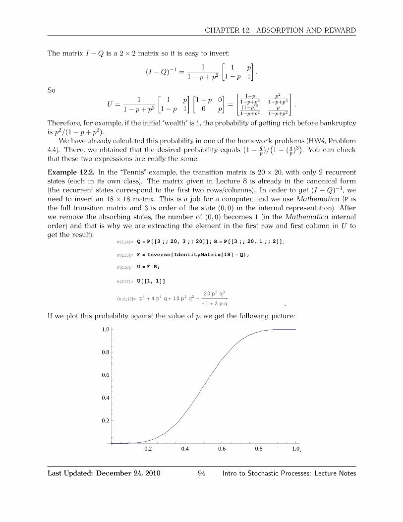
CHAPTER 12. ABSORPTION AND REWARD
The matrix I −Q is a 2× 2 matrix so it is easy to invert:
(I −Q)−1 =1
1− p+ p2
[1 p
1− p 1
].
So
U =1
1− p+ p2
[1 p
1− p 1
] [1− p 0
0 p
]=
[1−p
1−p+p2p2
1−p+p2(1−p)21−p+p2
p1−p+p2
].
Therefore, for example, if the initial “wealth” is 1, the probability of getting rich before bankruptcyis p2/(1− p+ p2).
We have already calculated this probability in one of the homework problems (HW4, Problem4.4). There, we obtained that the desired probability equals (1 − q
p)/(1 − ( qp)3
). You can check
that these two expressions are really the same.
Example 12.2. In the “Tennis” example, the transition matrix is 20 × 20, with only 2 recurrentstates (each in its own class). The matrix given in Lecture 8 is already in the canonical form(the recurrent states correspond to the first two rows/columns). In order to get (I − Q)−1, weneed to invert an 18 × 18 matrix. This is a job for a computer, and we use Mathematica (P isthe full transition matrix and 3 is order of the state (0, 0) in the internal representation). Afterwe remove the absorbing states, the number of (0, 0) becomes 1 (in the Mathematica internalorder) and that is why we are extracting the element in the first row and first column in U toget the result):
In[114]:= Q = P@@3 ;; 20, 3 ;; 20DD; R = P@@3 ;; 20, 1 ;; 2DD;
In[115]:= F = Inverse@IdentityMatrix@18D - QD;
In[116]:= U = F.R;
In[117]:= U@@1, 1DD
Out[117]= p4 + 4 p4 q + 10 p4 q2 - 20 p5 q3
-1 + 2 p q .
If we plot this probability against the value of p, we get the following picture:
0.2 0.4 0.6 0.8 1.0
0.2
0.4
0.6
0.8
1.0
.
Last Updated: December 24, 2010 94 Intro to Stochastic Processes: Lecture Notes

CHAPTER 12. ABSORPTION AND REWARD
12.2 Expected reward
Suppose that each time you visit a transient state j ∈ T you receive a reward g(j) ∈ R. The name“reward” is a bit misleading since the negative g(j) corresponds more to a fine than to a reward;it is just a name, anyway. Can we compute the expected total reward before absorption
vi = Ei[τC∑n=0
g(Xn)]?
And if we can, what is it good for? Many things, actually, as the following two special cases show:
1. If g(j) = 1 for all j ∈ T , then vi is the expected time until absorption. We will calculatev(0,0) for the “Tennis” example to compute the expected duration of a tennis game.
2. If g(k) = 1 and g(j) = 0 for j 6= k, then vi is the expected number of visits to the state kbefore absorption. In the “Tennis” example, if k = (40, 40), the value of v(0,0) is the expectednumber of times the score (40, 40) is seen in a tennis game.
We compute vi using the first-step decomposition:
vi = E[
τC∑n=0
g(Xn)|X0 = i] = g(i) + E[
τC∑n=1
g(Xn)|X0 = i]
= g(i) +∑k∈S
E[
τC∑n=1
g(Xn)|X0 = i,X1 = k]P[X1 = k|X0 = i]
= g(i) +∑k∈S
pikE[
τC∑n=1
g(Xn)|X1 = k]
(12.1)
If k ∈ T , then the homogeneity of the chain implies that
E[
τC∑n=1
g(Xn)|X1 = k] = E[
τC∑n=0
g(Xn)|X0 = k] = vk.
When k 6∈ T , then
E[
τC∑n=1
g(Xn)|X1 = k] = 0,
because we have “arrived” and no more rewards are going to be collected. Therefore, for i ∈ Twe have
vi = g(i) +∑k∈T
pikvk.
If we organize all vi and all g(i) into column vectors v = (vi, i ∈ T ), g = (g(i), i ∈ T ), we get
v = Qv + g, i.e., v = (I −Q)−1g.
Having derived the general forumla for various rewards, we can give an interpretation of thefundamental matrix itself. Let us pick a transient state j and use the reward function g given by
g(k) = 1k=j =
1, k = j
0, k 6= j.
Last Updated: December 24, 2010 95 Intro to Stochastic Processes: Lecture Notes

CHAPTER 12. ABSORPTION AND REWARD
By the discussion above, the ith entry in v = (I − Q)−1g is the expected reward when we startfrom the state i. Given the form of the reward function, vi is the expected number of visits tothe state j when we start from i. On the other hand, as the product of the matrix (I −Q)−1 andthe vector g = (0, 0, . . . , 1, . . . , 0), vi is nothing but the (i, j)-entry in (I −Q)−1:
Proposition 12.3. For two transient states i and j , the (i, j)-th entry in the fundamental matrix(I −Q)−1 is the expteced number of visits to the state j prior to absorbtion if the chain startsfrom the state i (the time 0 is counted, if i = j).
Example 12.4. We continue the analysis of the “Tennis” chain from Example 12.2. We set g(i) = 1for all transient states i to find the expected duration of a tennis game.
In[87]:= G = Table@81<, 8i, 1, 18<D;
In[86]:= f@p_D = [email protected]@@1, 1DD . 8q ® 1 - p<D
Out[86]= - 4 I-1 + p - p2 - 6 p3 + 18 p4 - 18 p5 + 6 p6M
1 - 2 p + 2 p2 .
We can plot this as a function of p to get the following graph:
0.0 0.2 0.4 0.6 0.8 1.0
4.0
4.5
5.0
5.5
6.0
6.5
7.0
.
When p = 0, the course of the game is totally predictable and Amélie wins in 4 points. The sameholds when p = 1, only it is Björn who wins with probabilty 1 this time. In between, we see thatthe expected game-length varies between 4 and about 7 (actually, the exact number is 6.75), andit longest when p = 1
2 .How about the expected number of deuces (scores (40, 40))? We can compute that too by set-
ting g(i) = 0 if i 6= (40, 40) and g((40, 40)) = 1 (the number 16 used below is just the Mathematica
Last Updated: December 24, 2010 96 Intro to Stochastic Processes: Lecture Notes

CHAPTER 12. ABSORPTION AND REWARD
internal number of the state (40,40) among the transient states):
In[117]:= G = Table@8If@i 16, 1, 0D<, 8i, 1, 18<D
Out[117]= 880<, 80<, 80<, 80<, 80<, 80<, 80<, 80<, 80<, 80<, 80<, 80<, 80<, 80<, 80<, 81<, 80<, 80<<
In[118]:= f@p_D = [email protected]@@1, 1DD . 8q ® 1 - p<D
Out[118]= - 20 H-1 + pL
3p3
1 - 2 p + 2 p2
The plot of the obtained expressions, as a function of p, looks like this
0.2 0.4 0.6 0.8 1.0
0.1
0.2
0.3
0.4
0.5
0.6
2 4 6 8
100
200
300
400
500
600
700
Therefore, the expected number of deucesvaries between 0 and a bit more than 0.6(the exact number is 0.625 and correspondsto the case p = 1
2 ). When asked, peoplewould usually give a higher estimate for thisprobability. The reason is that the distribu-tion of the number of deuces looks some-thing like the picture on the left (a his-togram of the number of deuces in a simu-lation of 1000 tennis games with p = 1
2 ). Wesee that most of the games have no deuces.However, in the cases where a deuce hap-pens, it is quite possible it will be repeated.
From a psychological point of view, we tend to forget all the games without deuces and focuson those with at least 1 deuce when we make predictions. In fact, the expected number of deucesgiven that the game contains at least one deuce is approximatly equal to 2.1.
Last Updated: December 24, 2010 97 Intro to Stochastic Processes: Lecture Notes

Chapter 13
Stationary and Limiting Distributions
Transitions between different states of a Markov chain describe short-time behavior of the chain.In most models used in physical and social sciences, systems change states many times persecond. In a rare few, the time scale of the steps can be measured in hours or days. What is ofinterest, however, is the long-term behavior of the system, measured in thousands, millions, oreven billions of steps. Here is an example: for a typical liquid stock traded on the New York StockExcahenge, there is a trade every few seconds, and each trade changes the price (state) of thestock a little bit. What is of interest to an investor is, however, the distribution of the stock-price in6 months, in a year or, in 30 years - just in time for retirement. A back-of-an-envelope calculationshows that there are, approximately, 50 million trades in 30 years. So, a grasp of very-long timebehavior of a Markov chain is one of the most important achievments of probability in general,and stochastic-process theory in particular. We only scratch the surface in this lecture.
13.1 Stationary and limiting distributions
Definition 13.1. A stochastic process Xnn∈N0 is said to be stationary if the random vectors
(X0, X1, X2, . . . , Xk) and (Xm, Xm+1, Xm+2, . . . , Xm+k)
have the same (joint) distribution for all m, k ∈ N0.
For stationary processes, all random variables X0, X1, . . . have the same distribution (justtake k = 0 in the definition). That condition is, however, only necessary. The pairs (X0, X1) and(Xm, Xm+1) should be equally distributed as random vectors, the same for triplets, etc. Intuitively,a stochastic process is stationary if, statistically, it does not evolve. Its probabilistic behavior todayis the same as its probabilistic behavior in a billion years. It is somethimes useful to think aboutstationarity in the following way; if a system is let to evolve for a long time, it will reach anequilibrium state and fluctuate around it forever. We can expect that such a system will looksimilar a million years from now and a billion years from now. It might, however, not resembleits present state at all. Think about a glass of water in which we drop a tiny drop of ink. Imediatelyafter that, the glass will be clear, with a tiny black speck. The ink starts to diffuse and the spackstarts to grow immediately. It won’t be long before the whole glass is of uniform black color - theink has permeated every last “corner” of the glass. After that, nothing much happens. The ink
98

CHAPTER 13. STATIONARY AND LIMITING DISTRIBUTIONS
will never spontaneously return to its initial state1. Ink is composed of many small particles whichdo not interact with each other too much. They do, however, get bombarded by the molecules ofwater, and this bombardment makes them behave as random walks which simply bounce backonce they hit the glass wall (this phenomenon is called diffusion). Each ink particle will wanderoff in its own direction, and quite soon, they will be “everywhere”. Eventally, the distribution ofthe ink in the glass becomes very close to uniform and no amount of further activity will changethat - you just cannot get more “random” then the uniform distribution in a glass of water.
Let us get back to mathematics and give two simple examples; one of a process which is notstationary, and the other of a typical stationary process.
Example 13.2. The simple random walk is not stationary. Indeed, X0 is a constant, while X1
takes two values with equal probabilities, so they cannot have the same distribution.For an example of a stationary process, take a regime switching chain Xnn∈N0 with p01 =
p10 = 1, and the initial distribution P[X0 = 0] = P[X0 = 1] = 12 . Then Xn = X0 if n is even, and
Xn = 1−X0 if n is odd. Moreover, X0 and 1−X0 have the same distribution (Bernoulli with p = 12 ),
and, so X0, X1, . . . all have the same distribution. How about k-tuples? Why do (X0, X1, . . . , Xk)and (Xm, Xm+1, . . . , Xm+k) have the same distribution? For i0, i1, . . . , ik ∈ 0, 1, by the Markovproperty, we have
P[X0 = i0, X1 = ii, . . . , Xk = ik] = P[X0 = i0]pi0i1pi1i2 . . . pik−1ik = 12pi0i1pi1i2 . . . pik−1ik .
In the same manner,
P[Xm = i0, X1 = ii, . . . , Xm+k = ik] = P[Xm = i0]pi0i1pi1i2 . . . pik−1ik = 12pi0i1pi1i2 . . . pik−1ik ,
so the two distributions are identical.
The second example above is quite instructive. We took a Markov chain and gave it aninitial distribution with the property that X0 and Xm have the same distribution for all m ∈ N0.Magically, the whole process became stationary. This is not a coincidence; we can play the sametrick with any Markov chain, as long as the initial distribution with the above property can befound. Actually, such a distribution is so important that it even has a name:
Definition 13.3. A distribution π = (πi)i∈S on the state space S of a Markov chain with transitionmatrix P is called a stationary distribution if
P[X1 = i] = πi for all i ∈ S, whenever P[X0 = i] = πi, for all i ∈ S.
In words, π is called a stationary distribution if the distribution of X1 is equal to that of X0
when the distribution of X0 is π. Here is a hands-on characterization:
Proposition 13.4. A vector π = (πi, i ∈ S) with∑
i∈S πi = 1 is a stationary distribution if andonly if
πP = π,
when π is interpreted as a row vector. In that case the Markov chain with initial distributionπ and transition matrix P is stationary and the distribution of Xm is π for all m ∈ N0.
1It will, actually, but it will take an unimaginably long time.
Last Updated: December 24, 2010 99 Intro to Stochastic Processes: Lecture Notes

CHAPTER 13. STATIONARY AND LIMITING DISTRIBUTIONS
Proof. Suppose, first, that π is a stationary distribution, and let Xnn∈N0 be a Markov chain withinitial distribution a(0) = π and transition matrix P . Then,
a(1) = a(0)P = πP.
By the assumption, the distribution a(1) of X1 is π. Therefore, π = πP .Conversely, suppose that π = πP . We can directly prove more than just the fact that π is a
stationary distribution. We can prove that the process Xnn∈N0 is stationary. Let Xnn∈N0 be aMarkov chain with initial distribution π and transition matrix P . We need to show that Xnn∈N0
is stationary. In order to do that, we first note that all random variables Xm, m ∈ N0, have thesame distribution. Indeed, the distribution a(m) of Xm is given by
a(m) = a(0)Pm = πPm = (πP )Pm−1 = πPm−1 = · · · = π.
Next, we pick m, k ∈ N0 and a k+ 1-tuple i0, i1, . . . , ik of elements of S . By the Markov property,we have
P[Xm = i0, Xm+1 = i1, . . . , Xm+k = ik] = P[Xm = i0]pi0i1pi1i2 . . . pik−1ik = πi0pi0i1pi1i2 . . . pik−1ik .
This last expression does not depend on m, so we can conclude that Xnn∈N0 is stationary.
Example 13.5 (A model of diffusion in a glass). Let us get back to the story about the glass ofwater and let us analyze a simplified model of that phenomenon. Our glass will be representedby the set 0, 1, 2, . . . , a, where 0 and a are the positions adjacent to the walls of the glass. Theink particle performs a simple random walk inside the glass. Once it reaches the state 0 it eithertakes a step to the right to 1 (with probability 1
2 ) or tries to go left (also with probability 12 ). The
passage to the left is blocked by the wall, so the particle ends up staying where it is. The samething happens at the other wall. All in all, we get a Markov chain with the following transitionmatrix
P =
12
12 0 0 . . . 0 0 0
12 0 1
2 0 . . . 0 0 00 1
2 0 12 . . . 0 0 0
......
...... . . . ...
......
0 1 0 0 . . . 0 12 0
0 1 0 0 . . . 12 0 1
20 1 0 0 . . . 0 1
212
.
Let us see what happens when we start the chain with a distribution concentrated in a/2 (assumingthat a is even); a graphical representation of the distribution of X3, X12, X30, X200, X700 and X5000
when a = 30 represents the behavior of the system very well (the y axis is on a different scaleson the first two plots):
0 5 10 15 20 25 30
0.2
0.4
0.6
0.8
1.0
0 5 10 15 20 25 30
0.2
0.4
0.6
0.8
1.0
0 5 10 15 20 25 30
0.05
0.10
0.15
0.20
Last Updated: December 24, 2010 100 Intro to Stochastic Processes: Lecture Notes

CHAPTER 13. STATIONARY AND LIMITING DISTRIBUTIONS
0 5 10 15 20 25 30
0.05
0.10
0.15
0.20
0 5 10 15 20 25 30
0.05
0.10
0.15
0.20
0 5 10 15 20 25 30
0.05
0.10
0.15
0.20
How about if we start from a different initial distribution? Here are the same plots in thatcase:
0 5 10 15 20 25 30
0.2
0.4
0.6
0.8
1.0
0 5 10 15 20 25 30
0.2
0.4
0.6
0.8
1.0
0 5 10 15 20 25 30
0.05
0.10
0.15
0.20
0 5 10 15 20 25 30
0.05
0.10
0.15
0.20
0 5 10 15 20 25 30
0.05
0.10
0.15
0.20
0 5 10 15 20 25 30
0.05
0.10
0.15
0.20
As you can see, the distribution changes rapidly at first, but then, once it has reached the“equilibrium” it changes remarkably little (compare X700 and X5000). Also, the “equilibrium”distribution is very uniform and does not depend on the initial distribution; this is exactly whatyou would expect from a long-term distribution of ink in a glass.
Let us show that the uniform distribution π = (1/(a+1), 1/(a+1), . . . , 1/(1+a)) = (1/31, 1/31, . . . , 1/31)on 0, 1, 2, . . . , a is indeed the (unique) stationary distribution. By Proposition 13.4, we need tosolve the equation π = Pπ. If we write out this system of equations line by line, we get
π0 = 12(π0 + π1)
π1 = 12(π0 + π2)
π2 = 12(π1 + π3)
π3 = 12(π2 + π4)
...πa−1 = 1
2(πa−2 + πa)
πa = 12(πa−1 + πa)
(13.1)
The first equation yields π0 = π1. Using that in the second one, we get π1 = π2, etc. Finally, weknow that π is a probability distribution so that π0 + π1 + · · ·+ πa = 1. Therefore, πi = 1/(a+ 1)for all i ∈ S , i.e., the uniform distribution on S is the only stationary distribution.
Last Updated: December 24, 2010 101 Intro to Stochastic Processes: Lecture Notes

CHAPTER 13. STATIONARY AND LIMITING DISTRIBUTIONS
Can there be more than one stationary distribution? Can there be none? Sure, here is anexample:
Example 13.6. For P = I , any distribution is stationary, and there are infinitely many.A simple example where no stationary distribution exists can be constructed on an infinite
state space. Take the Deterministically Monotone Markov Chain. The transition “matrix” lookslike the identity matrix, with the diagonal of ones shifted to the right. Therefore, the system ofequations π = πP reads
π1 = π2, π2 = π3, . . . , πn = πn+1, . . . ,
and so, for π to be a stationary distribution, we must have πn = π1 for all n ∈ N. Now, if π1 = 0,π is not a distribution (it sums to 0, not 1). But if π1 > 0, then the sum is +∞, so π is not adistribution either. Intuitively, the chain never stabilizes, it just keeps moving to the right adinfinitum.
The example with many stationary distributions can be constructed on any state space, but theother one, where no stationary distribution exists, had to use an infinite one. Was that necessary?Yes. Before we show this fact, let us analyze the relation between stationary distributions and theproperties of recurrence and transience. Here is our first result:
Proposition 13.7. Suppose that the state space S of a Markov chain is finite and let S =C1 ∪ C2 ∪ · · · ∪ Cm ∪ T be its canonical decomposition, Then the following two statements areequivalent:
1. π is a stationary distribution, and
2. πCk = πCkPk , k = 1, . . . ,m, and πT = (0, 0, . . . , 0),
where
P =
P1 0 0 0... . . . ... 00 0 Pm 0
R Q
,is the canonical form of the transition matrix, πCk = (πi, i ∈ Ck), k = 1, 2, . . . ,m and πT =(πi, i ∈ T ).
Proof. We write the equation π = πP coordinatewise as πj =∑
i∈S πipij and, by distinguishingthe cases i ∈ Ck , k ∈ 1, 2, . . . ,m, and i ∈ T , we get the following sytem of matrix equations(alternatively, just write the system π = πP in the block-matrix form according to the cannonicaldecomposition above):
πCk = πCKPCk
+ πTR, k = 1, . . . ,m, and πT = πTQ.
The last equality can be read as follows: πT is in a row null-space of I −Q. We know, however,that I −Q admits an inverse, and so it is a regular square matrix. Its row null-space (as well asits column null-space) must be trivial, and, consequently, πT = 0.
Having established that πT = 0, we can de-couple the system of equations above and write itas
πCk = πCKPk, k = 1, . . . ,m, and πT = (0, 0, . . . , 0),
Last Updated: December 24, 2010 102 Intro to Stochastic Processes: Lecture Notes

CHAPTER 13. STATIONARY AND LIMITING DISTRIBUTIONS
which is exactly what we needed to prove.The other implication - the proof of which consists of a verification of the fact that each
distribution from (2) above is indeed a stationaty distribution - is left to the reader.
The moral of the story of Proposition 13.7 is the following: in order to compute the stationarydistribution(s), classify the states and find the canonical decomposition of the state space. Then,set πi = 0 for any transient state i. What remains are recurrent classes, and you can analyizeeach one separately. Note, however, that πCk does not need to be a real distribution on Ck , since∑
i∈CkπCki does not need to equal 1. However, unless πCk = (0, 0, . . . , 0), we can always multiply
all its elements by a constant to make the sum equal to 1.Thanks to the results of Proposition 13.7, we can focus on Markov chains with only one class:
Definition 13.8. A Markov chain is said to be irreducible if there is only one class.When a Markov chain is finite and irreducible, all of its states must be recurrent. Indeed, a
finite Markov chain has at least one recurrent state, and recurrence is a class property.Now that we have described the structure of the set of all stationary distributions, we still
need to to tackle the question of existence: are there any stationary distributions? In additionto giving an affirmative answer to this question, we will also show how to construct a stationarydistribution and how to interpret it probabilistically.Proposition 13.9. Let Xnn∈N0 be an irreducible Markov chain with a finite state space. Then,the following two statements hold:
1. All states are positive recurrent.
2. Let i be a fixed (but arbitrary) recurrent state. Let
νj = Ei
τi(1)−1∑n=0
1Xn=j
, j ∈ Sbe the expected number of visits to state j in between two consecutive visits to statei. Then the vector π, given by πj = 1
miνj , j ∈ S (where mi = Ei[τi(1)] ) is a stationary
distribution.Remark 13.10. Even though it is not exceedingly hard, the proof of this proposition is a bittechnical, so we omit it. It is important, however, to understand what the propositions states:
1. the expected number of visits to the state j in between two consecutive visits to the state ican be related to a stationary distribution of the Markov chain by νj = miπj , and
2. when we set j = i, νi counts the number of visits to i between two consecutive visits toi, which is always equal to 1 (the first visit is counted and the last one is not). Therefore,νi = 1, and so πi = 1
mi.
Proposition 13.9 and Remark 13.10 are typically used in the following way: one computesthe unique stationary distribution π by solving the equation π = πP and then draws conclusionsabout mi or the νj ’s.
Note also that the computation above is not a special case of a reward computation of theprevious lecture. There, you need to start from a transient state and finish in a recurrent state,while here your starting and final state are the same.
Last Updated: December 24, 2010 103 Intro to Stochastic Processes: Lecture Notes
CHAPTER 13. STATIONARY AND LIMITING DISTRIBUTIONS
13.2 Limiting distributions
Example 13.5 shows vividly how the distribution of ink quickly reaches the uniform equilibriumstate. It is no coincidence that this “limiting” distribution happens to be a stationaty distribution.Before we make this claim more precise, let us define rigorously what we mean by a limitingdistribution:
Definition 13.11. A distribution π = (πi, i ∈ S) on the state space S of a Markov chain withtransition matrix P is called a limiting distribution if
limn→∞
p(n)ij = πj ,
for all i, j ∈ S .
Note that for π to be a limiting distribution, all the limits in Definition 13.11 must exist. Oncethey do, π is automatically a distribution: πj ≥ 0 (as a limit of non-negative numbers) and∑
j∈Sπj =
∑j∈S
limn→∞
p(n)ij = lim
n→∞
∑j∈S
p(n)ij = lim
n→∞1 = 1.
Also, note that the independence on the initial state i is built into the definition of the limitingdistribution: the sequence p(n)ij n∈N must tend to the same limit πj for all i ∈ S . Moreover, itfollows immediately there can be at most one limiting distribution.
The connection with stationary distributions is spelled out in the following propositions:
Proposition 13.12. Suppose that a Markov chain with transition matrix P admits a limitingdistribution π = (πi, i ∈ S). Then π is a stationary distribution.
Proof. To show that π is a stationary distribution, we need to verify that it satisfies π = πP , i.e.,that
πj =∑i∈S
πipij .
We use the Chapman-Kolmogorov relation p(n+1)ij =
∑k∈S pikp
(n)kj and start from the observation
that πj = limn→∞ p(n+1)ij to get exactly what we need:
πj = limn→∞
p(n+1)ij = lim
n→∞
∑k∈S
p(n)ik pkj =
∑k∈S
( limn→∞
p(n)ik )pkj =
∑k∈S
πkpkj .
Example 13.13. Limiting distributions don’t need to exist, even when there are stationary ones.Here are two examples:
1. Let Xnn∈N0 be a Regime-switching chain with
P =
[0 11 0
]
Last Updated: December 24, 2010 104 Intro to Stochastic Processes: Lecture Notes

CHAPTER 13. STATIONARY AND LIMITING DISTRIBUTIONS
Then
p(n)ij =
12(1 + (−1)n), i = j12(1 + (−1)n+1), i 6= j.
Clearly, the sequence p(n)ij is alternating between 0 and 1, so it cannot admit a limit. A
stationary distribution exists: the system π = πP becomes
π0 = 0× π0 + 1× π1,π1 = 1× π0 + 0× π1.
2. In the previous example the limiting distribution did not exist which implies that π0 = π1.In order for π to be a distribution on 0, 1, we must have π0 = π1 = 1
2 . So, (12 ,12) is a
stationary distribution.
3. In the previous example the limiting distribution did not exists because the limits of thesequences p(n)ij did not exist. Another reason for the non-existence of limiting distributionscan be dependence on the initial conditions: the limits limn p
(n)ij may exist for all i, j , but
their values can depend on the intial state i. The simplest example is a Markov chain withtwo states i = 1, 2, where p11 = p22 = 1. There are two recurrent (and therefore closed)classes, and the chain remains in the state it starte in forever. Therefore, limn p
(n)12 = 0 and
limn p(n)22 = 1, so no limiting distribution exists despite the fact that all limits limn p
(n)ij do.
Proposition 13.14. Let Xnn∈N0 be a finite-state, irreducible and aperiodic Markov chain.Then the limiting distribution exists.
We conclude the discussion of limiting distributions with a version of the Law of LargeNumbers (LLN) for Markov chains. Before we state it, we recall the classical LLN for independentvariables:
Theorem 13.15. Let Xnn∈N0 be a sequence of independent and identically distributed randomvariables, such that E[|X0|] <∞. Then
limn
1
n
n−1∑k=0
Xk = E[X0],
almost surely 2.
When Xnn∈N0 is a Markov chain, two problems occur. First, the random variablesX0, X1, . . .are not independent. Second, Xk takes its values in the state space S which does not necessarilyconsist of numbers, so the expression X0 + X1 or E[X0] does not make sense all the time. Todeal with the second problem, we pick a numerical function f : S → R (give each state a value)and form sums of the form f(X0) + f(X1) + · · ·+ f(Xn−1). Independence is more subtle, but itcan be replaced with stationarity (loosely speaking), as in the following proposition (we skip theproof):
2Almost surely means with probability one, and states that this statement is true all the time for all practicalpurposes. It may fail, but only in extremely exceptional cases such as the one where you toss a fair coin infinitelymany times and get tails every single time. That means never, really.
Last Updated: December 24, 2010 105 Intro to Stochastic Processes: Lecture Notes

CHAPTER 13. STATIONARY AND LIMITING DISTRIBUTIONS
Proposition 13.16. Let Xnn∈N0 be an irreducible Markov chain with a finite state space S ,let π = (πi, i ∈ S) be the (unique) stationary distribution, and let f : S → R be an arbitraryfunction. Then
limn
∑n−1k=0 f(Xk)
n=∑i∈S
f(i)πi,
almost surely, no matter what initial distribution we choose.
Example 13.17. Let Xnn∈N0 be an irreducible finite Markov chain, and let the function f : S →R be given by
f(j) = 1(i=j) =
1, j = i,
0, j 6= i.
Then, by the Law of Large Numbers, we gave
limn
1
n
n−1∑k=0
1Xk=i =∑j∈S
1(i=j)πj = πi,
so that πi can be interpreted as a long-run percentage of time that the Markov chain Xnn∈N0
spends in the state i.
Last Updated: December 24, 2010 106 Intro to Stochastic Processes: Lecture Notes