introduction to stochastic optimization methods (meta...

Modern optimization methods 1

Introduction to Stochastic Optimization Methods

(meta-heuristics)


Efficiency of optimization methods

kombinatorial unimodal multimodal

Problem type

Efficiency

Specialized method

Enumeration or MC

Robust method


Classification of optimization methods


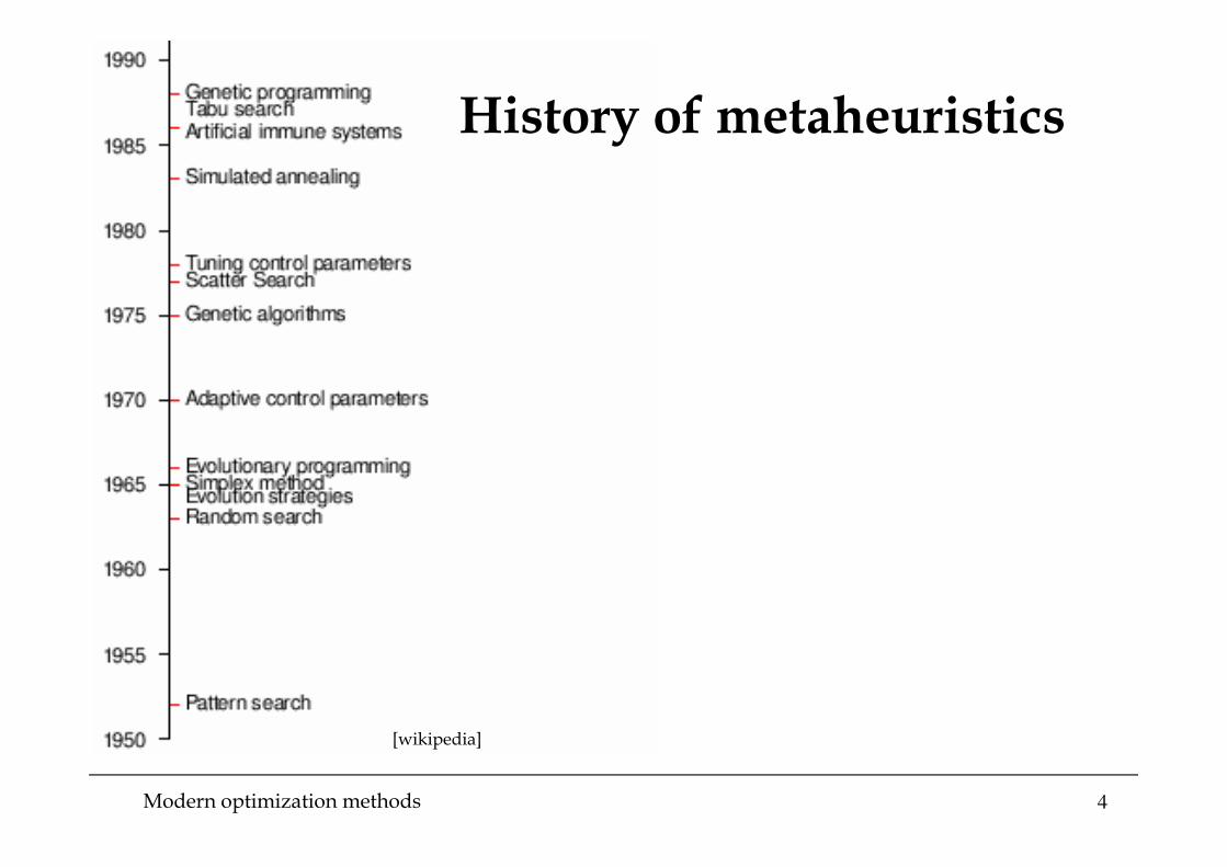
History of metaheuristics

[wikipedia]


Direct search methods

• Without knowledge of gradients (zero-order methods)

• Heuristics:– „... a heuristic is an algorithm that ignores whether the solution to the

problem can be proven to be correct, but which usually produces a good solution or solves a simpler problem that contains or intersects with the solution of the more complex problem. Heuristics are typically used when there is no known way to find an optimal solution, or when it is desirable to give up finding the optimal solution for an improvement in run time.“ [Wikipedia]

– For instance: Nelder-Mead algorithm

• Metaheuristics:– „designates a computational method that optimizes a problem by iteratively trying to improve a candidate solution.“ [Wikipedia]


Nelder-Mead method

• Heuristic method• Known also as a simplex method• Suitable for Dim<10


Nelder-Mead method

[Gioda & Maier, 1980]


Nelder-Mead method

0) original triangle, 1) expansion, 2) reflexion, 3) outer contraction, 4) inner

contraction, 5) reduction [Čermák & Hlavička, VUT, 2006]


Nelder-Mead method


Meta-heuristic

• Also called stochastic optimization methods–usage of random numbers => random behavior

• Altering of existing solutions by local change• Examples:

– Monte Carlo method– Dynamic Hill-climbing algorithm– Simulated Annealing, Threshold Acceptance– Tabu Search


Monte Carlo method

• Or „blind algorithm“• Serve as a benchmark

1 t = 02 Create P, evaluate P3 while (not stopping_criterion) {

4 t = t+15 Randomly create N, evaluate N6 If N is better than P, then P=N

7 }

also (brute-force search)


Global view on optimization


Local view on optimization


Hill-climbing algorithm

• Search in the vicinity of the current solution

x

�(�)max �(�)


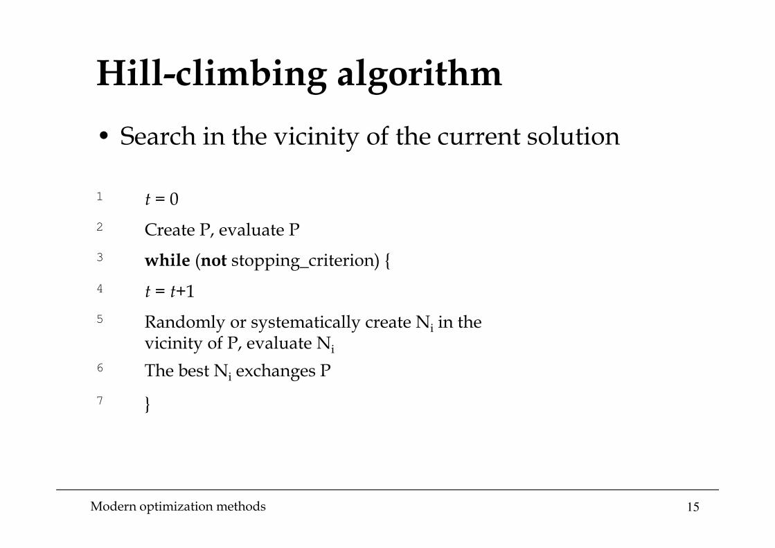
Hill-climbing algorithm

• Search in the vicinity of the current solution

1 t = 02 Create P, evaluate P3 while (not stopping_criterion) {

4 t = t+15 Randomly or systematically create Ni in the

vicinity of P, evaluate Ni

6 The best Ni exchanges P

7 }


Simulated annealing (SA)

• Discovered in 80’s independently by two authors[Kirkpatrick et al., 1983] and [Černý, 1985].

• Based on physical meaning, on an idea of annealing of metals, where the slow cooling leads material to the state of minimum energy. This is equivalent to the global minimization.

• There is a mathematical proof of convergence.


Physical background

• Theory based on monitoring of metallic crystals at different temperatures

High temperature Low temperature


Principles of method

• stochastic optimization method

• Probability to escape fromlocal minima

• consecutive decreasingof temperature,so-called cooling schedule

∆−=

T

EE

Bκexp)Pr(


Průběh tradičního vzorce pro různé teploty

0,00

0,20

0,40

0,60

0,80

1,00

1,20

1,40

1,60

1,80

-5 0 5 10 15 20 25

∆∆∆∆E

Pr

5 4 3 2 1 0,5

Temperature influence

• Probability

∆−=

T

EE

Bκexp)Pr(


Algorithm1 T = Tmax, Create P, evaluate P2 while (not stopping_criterion) { 3 count = succ = 04 while ( count < countmax & succ < succmax ) {5 count = count + 16 alter P by operator O, result is N7 p = exp ((F(N) − F(P))/T) (application of probability)

8 if ( random number u[0, 1] < p) {9 succ = succ + 110 P=N11 }if}while

12 Decrease T (cooling schedule)

13 }while


Algorithm

• Initial temperature Tmax is recommended at the level of e.g. 50% probability of acceptance of random solution. This leads to experimental investigation employing usually the “trial and error method”

• Parameter countmax is for maximal number of all iteration and succmax is the number of successful iterations at the fixed temperature level (so-called Markov chain). Recommended ration is countmax = 10 succmax


Algorithm

• Stopping criterion is usually the maximum number of function calls

• As an „mutation“ operator, the addition of Gaussian random number with zero mean is usually used, i.e.

N = P + G(0,σ) ,

where the standard deviation σ is usually obtained by the trial and error method


Cooling algorithms

• Classical: Ti+1 = TmultTi

• Where Tmult =0,99 or 0,999

• Other possibilities exist. e.g.:

see e.g. [Ingber]

• These settings usually do not provide flexibility to control the algorithm


Cooling algorithms

• Proposed methodology [Lepš, MSc. Thesis] [Lepš,Šejnoha]

• This relationship enables at maximum iterations itermaxreach the minimal temperature Tmin given by

Tmin = 0,01Tmax

• For instance: for succmax/itermax = 0,001 is Tmult=0,995


Note on probability

• For population based algorithms:

∆+

=

T

EE

Bκexp1

1)Pr(

Porovnání vzorců pro T=10

0,0

0,5

1,0

1,5

-5 -4 -3 -2 -1 0 1 2 3 4 5

∆∆∆∆E

PR

p=e^(-E/T) p=1/(1+e^(E/T))


SA convergence


Threshold acceptance

• Simpler than SA

• Instead of probability, there is a threshold, or range, within which the worst solution can replace the old one

• Threshold is decreasing similarly as temperature in SA

• There is a proof that this method does not ensure finding the global minima.


References[1] Kirkpatrick, S., Gelatt, Jr., C., and Vecchi, M. P. (1983).

Optimization by Simulated Annealing. Science, 220:671–680.

[2] Černý, J. (1985). Thermodynamical approach to the traveling salesmanproblem: An efficient simulation algorithm. J. Opt. Theory Appl., 45:41–51.

[3] Ingber, L. (1993). Simulated annealing: Practice versus theory. Mathematical and Computer Modelling, 18(11):29–57.

[4] Ingber, L. (1995). Adaptive simulated annealing (ASA): Lessons learned. Control and Cybernetics, 25(1):33–54.

[5] Vidal, R. V. V. (1993). Applied Simulated Annealing, volume 396 of Notes in Economics and Mathematical Systems. Springer-Verlag.


References[6] J. Dréo, A. Pétrowski, P. Siarry, E. Taillard, A. Chatterjee (2005).

Metaheuristics for Hard Optimization: Methods and Case Studies. Springer.

[7] M. Lepš and M. Šejnoha: New approach to optimization of reinforced concrete beams. Computers & Structures, 81 (18-19), 1957-1966, (2003).

[8] Burke, Edmund K., and Graham Kendall. Search methodologies. Springer Science+ Business Media, Incorporated, 2005.

[9] Weise, Thomas, et al. "Why is optimization difficult?" Nature-Inspired Algorithms for Optimisation. Springer Berlin Heidelberg, 2009. 1-50.

[10] S. Venkataraman and R.T. Haftka: Structural optimization complexity: What has Moore’s law done for us? Struct Multidisc Optim 28, 375–387 (2004).


Travelling Salesman problem (TSP)

• One of the most famous discrete optimization problems

• The goal is to find closed shortest path in edge-oriented weighted graph

• For n cities, there are (n–1) ! /2 possible solutions

• NP-complete task



34

A B

C D

20

12

42

3035

A B C D

A 0 20 42 35

B 20 0 30 34

C 42 30 0 12

D 35 34 12 0

• Example



No. Order of the city distance

1 2 3 4

I. A B C D 97

II. A B D C 108

III. A C B D 141

34

A B

C D

20

12

42

3035

34

A B

C D

20

12

42

3035

34

A B

C D

20

12

42

3035

Solution I. Solution II. Solution III.



No. cities Possible paths Computational demands

4 3 3,0 · 10-09 seconds

5 12 1,2 · 10-08 seconds

6 60 6,0 · 10-08 seconds

7 360 3,6 · 10-07 seconds

8 2520 2,5 · 10-06 seconds

9 20160 2,0 · 10-05 seconds

10 181440 1,8 · 10-04 seconds

20 6,1 · 1016 19,3 years

50 3,0 · 1062 9,6 · 1046 years

100 4,7 · 10157 1,5 · 10140 years

Based on 109 operations per 1 second computer speed



The OPTNET Procedure 1 Mathematica software2

1 http://support.sas.com/documentation/cdl/en/ornoaug/65289/HTML/default/viewer.htm#ornoaug_optnet_examples07.htm2 http://mathematica.stackexchange.com/questions/15985/solving-the-travelling-salesman-problem

http://gebweb.net/optimap/


Example

• tsp.m


Local operator


A humble plea. Please feel free to e-mail any suggestions, errors andtypos to [email protected].

Date of the last version: 10.11.2015

Version: 003

News 21.10.2013: Added Nelder-Mead method and the introduction redone.

News 5.11.2014: Added TSP after the end.

News 10.11.2015: Enhancement of TSP.

Some parts of this presentation have been kindly prepared by Ing. Adéla

Pospíšilová with Faculty of Civil Engineering, CTU in Prague.

introduction to stochastic optimization methods (meta...

Documents