introduction to qcd and jet ii

Introduction to QCD and Jet II

Bo-Wen Xiao

Pennsylvania State Universityand Institute of Particle Physics, Central China Normal University

Jet Summer SchoolMcGill June 2012

1 / 56

Outline

1 Collinear Factorization and DGLAP equationTransverse Momentum Dependent (TMD or kt) Factorization

2 Introduction to Small-x PhysicsBFKL evolution and Balitsky-Kovchegov evolution equationsMcLerran-Venugopalan Model

3 Dihadron CorrelationsBreaking down of the kt factorization in di-jet productionProbing two fundamental gluon distributionsGluon+Jet in pA

2 / 56

Collinear Factorization and DGLAP equation

Deep inelastic scattering and Drell-Yan process

3 / 56


Light Cone coordinates and gauge

For a relativistic hadron moving in the +z direction

Motivation

Dipole picture for DIS

Non–linear evolution: BK!Bremsstrahlung!BFKL Evolution! Light Cone!Dipole splitting!Dipole evolution!Balitsky equation!BK equation

SCHOOL ON QCD, LOW X PHYSICS, SATURATION AND DIFFRACTION: Copanello (Calabria, Italy), July 1 - 14 2007 Non–linear evolution & Gluon saturation in QCD at high energy (I) – p. 25

Light Cone notations & Kinematics" The hadron moves in the positive z direction, with v c = 1

" Longitudinal momentum P M =⇒ Pµ = (E ≈ P, 0, 0, P )

P+ ≡ 1√2(E + P )

√2P , P− ≡ 1√

2(E − P ) 0

" Even for the quantum system, the wavefunction is stronglylocalized near x− = 0 (“pancake”)

∆x− ∼ 1

P+∼ 1

γM 1

M

In this frame, the momenta are defined

P+ =

1√

2(P0 + P

3) and P− =

1√

2(P0

− P3) → 0

P2 = 2P

+P−− P

2⊥

Light cone gauge for a gluon with momentum kµ = (k+, k

−, k⊥), the polarization vectorreads

kµµ = 0 ⇒ = (+ = 0, − =

⊥ · k⊥

k+, ±⊥) with ±⊥ =

1√

2(1,±i)

4 / 56


Deep inelastic scattering

Summary of DIS:dσ

dEdΩ=

αem2

Q4E

ELµνW

µν

with Lµν the leptonic tensor and Wµν defined as

Wµν =

−g

µν +qµqν

q2

W1

+1

m2p

Pµ−

P · q

q2 qµ

Pν−

P · q

q2 qν

W2

Introduce the dimensionless structure function:

F1 ≡ W1 and F2 ≡Q

2

2mpxW2

⇒dσ

dxdy=

α2em4πs

Q4

(1 − y)F2 + xy

2F1

with y =

P · q

P · k.

Quark Parton Model: Callan-Gross relation

F2(x) = 2xF1(x) =

q

e2qx [fq(x) + fq(x)] .

5 / 56


Callan-Gross relation

The relation (FL = F2 − 2xF1) follows from the fact that a spin- 12 quark cannot absorb a

longitudinally polarized vector boson.In contrast, spin-0 quark cannot absorb transverse bosons and so would give F1 = 0.

6 / 56


Parton Density

The probabilistic interpretation of the parton density.

⇒ fq(x) =

dζ−

4πe

ixP+ζ−

Pψ(0)γ+ψ(0, ζ−)

P

Comments:Gauge link L is necessary to make the parton density gauge invariant.

L(0, ζ−) = P exp

ζ−

0dsµA

µ

Choose light cone gauge A+ = 0 and right path, one can eliminate the gauge link.

Now we can interpret fq(x) as parton density in the light cone frame.Evolution of parton density: Change of resolution

13J.Pawlowski / U. Uwer

Advanced Particle Physics: VII. Quantum Chromodynamics

QCD explains observed scaling violation

Large x: valence quarks Small x: Gluons, sea quarks

Q2 F2 for fixed x Q2 F2 for fixed x

Scaling violation is one of the clearest manifestation of radiative effect predicted by QCD.

Quantitative description of scaling violation

)()()()( 21

0

22 xqexdxqexxF i

ii

iii

P

Quark Parton Model

QCD

P

x/xz

)log()(P2

~

)(P2

~

20

2

qq

2

2

qq

2

20

Qz

kdkz

s

Q

T

Ts

Tkk,

20

21

0

222 log)(P

2)1()(),(

Qxxq

dexQxF qq

s

iii

Pqq probability of a quark to emit gluon and becoming a quark with momentum reduced by fraction z.

0 cutoff parameter

MQx

2

2

)(1

)( xa

ax

x

x x

At low-x, dominant channels are different.7 / 56


Drell-Yan process

For lepton pair productions in hadron-hadron collisions:

the cross section isdσ

dM2dY=

q

x1fq(x1)x2fq(x2)13

e2q

4πα2

3M4 with Y =12

lnx1

x2.

Collinear factorization proof shows that fq(x) involved in DIS and Drell-Yan process arethe same.At low-x and high energy, the dominant channel is qg → qγ∗(l+l

−).

g

qγ∗

l

l

8 / 56


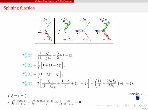
Splitting function

P0qq(ξ) =

1 + ξ2

(1 − ξ)++

32δ(1 − ξ),

P0gq(ξ) =

1ξ

1 + (1 − ξ)2

,

P0qg(ξ) =

(1 − ξ)2 + ξ2

,

P0gg(ξ) = 2

ξ

(1 − ξ)++

1 − ξξ

+ ξ(1 − ξ)

+

116

−2Nf TR

3Nc

δ(1 − ξ).

ξ = z = x

y.

10

dξf (ξ)(1−ξ)+

= 1

0dξ[f (ξ)−f (1)]

1−ξ ⇒ 1

0dξ

(1−ξ)+= 0

9 / 56


Derivation of P0qq(ξ)

The real contribution:

1

2

3

k1 = (P+, 0, 0⊥) ; k2 = (ξP+,

k2⊥

ξP+, k⊥)

k3 = ((1 − ξ)P+,k

2⊥

(1 − ξ)P+,−k⊥) 3 = (0,−

2k⊥ · (3)⊥

(1 − ξ)P+, (3)

⊥ )

|Vq→qg|2 =12

Tr (/k2γµ/k1γν)

∗µ3 ν3 =2k

2⊥

ξ(1 − ξ)

1 + ξ2

1 − ξ

⇒ Pqq(ξ) =1 + ξ2

1 − ξ(ξ < 1)

Including the virtual graph , use 1

a

dξg(ξ)(1−ξ)+

= 1

a

dξg(ξ)1−ξ − g(1)

10

dξ1−ξ

αsCF

2π

1

x

dξξ

q(x/ξ)1 + ξ2

1 − ξ− q(x)

1

0dξ

1 + ξ2

1 − ξ

=αsCF

2π

1

x

dξξ

q(x/ξ)1 + ξ2

(1 − ξ)+− q(x)

1

0dξ

1 + ξ2

(1 − ξ)+

=− 3

2

.

10 / 56


Derivation of P0qq(ξ)

The real contribution:

1

2

3

k1 = (P+, 0, 0⊥) ; k2 = (ξP+,

k2⊥

ξP+, k⊥)

k3 = ((1 − ξ)P+,k

2⊥

(1 − ξ)P+,−k⊥) 3 = (0,−

2k⊥ · (3)⊥

(1 − ξ)P+, (3)

⊥ )

|Vq→qg|2 =

12

Tr (/k2γµ/k1γν)

∗µ3 ν3 =2k

2⊥

ξ(1 − ξ)1 + ξ2

1 − ξ

⇒ Pqq(ξ) =1 + ξ2

1 − ξ(ξ < 1)

Regularize 11−ξ to 1

(1−ξ)+by including the divergence from the virtual graph.

Probability conservation:

Pqq + dPqq = δ(1 − ξ) +αsCF

2πP

0qq(ξ)dt and

1

0dξPqq(ξ) = 0,

⇒ Pqq(ξ) =1 + ξ2

(1 − ξ)++

32δ(1 − ξ) =

1 + ξ2

1 − ξ

+

.

11 / 56


Derivation of P0gg(ξ)

1

2

3

k1 = (P+, 0, 0⊥) 1 = (0, 0, (1)⊥ ) with ±⊥ =

1√2(1,±i)

k2 = (ξP+,

k2⊥

ξP+, k⊥) 2 = (0,

2k⊥ · (2)⊥

ξP+, (2)

⊥ )

k3 = ((1 − ξ)P+,k

2⊥

(1 − ξ)P+,−k⊥) 3 = (0,−

2k⊥ · (3)⊥

(1 − ξ)P+, (3)

⊥ )

Vg→gg = (k1 + k3) · 21 · 3 + (k2 − k3) · 12 · 3 − (k1 + k2) · 31 · 2

⇒ |Vg→gg|2 = |V+++|

2 + |V+−+|2 + |V++−|

2 = 4k2⊥[1 − ξ(1 − ξ)]2

ξ2(1 − ξ)2

⇒ Pgg(ξ) = 2

1 − ξξ

+ξ

1 − ξ+ ξ(1 − ξ)

(ξ < 1)

Regularize 11−ξ to 1

(1−ξ)+Momentum conservation:

1

0dξ ξ [Pqq(ξ) + Pgq(ξ)] = 0

1

0dξ ξ [2Pqg(ξ) + Pgg(ξ)] = 0,

⇒ the terms which is proportional to δ(1 − ξ).HW: derive other splitting functions. 12 / 56


DGLAP equation

In the leading logarithmic approximation with t = lnµ2, the parton distribution andfragmentation functions follow the DGLAP[Dokshitzer, Gribov, Lipatov, Altarelli, Parisi,1972-1977] evolution equation as follows:

ddt

q (x, µ)g (x, µ)

=

α (µ)2π

1

x

dξξ

CFPqq (ξ) TRPqg (ξ)CFPgq (ξ) NcPgg (ξ)

q (x/ξ, µ)g (x/ξ, µ)

,

and

ddt

Dh/q (z, µ)Dh/g (z, µ)

=

α (µ)2π

1

z

dξξ

CFPqq (ξ) CFPgq (ξ)TRPqg (ξ) NcPgg (ξ)

Dh/q (z/ξ, µ)Dh/g (z/ξ, µ)

,

Comments:In the double asymptotic limit, Q

2→ ∞ and x → 0, the gluon distribution can be solved

analytically and cast into

xg(x, µ2) exp

2

αsNc

πln

1x

lnµ2

µ20

Fixed coupling

xg(x, µ2) exp

2

Nc

πbln

1x

lnlnµ2/Λ2

lnµ20/Λ

2

Running coupling

The full DGLAP equation can be solved numerically.13 / 56


Collinear Factorization at NLO

PDF PDF

FF FF

P P

h

Use MS scheme ( 1 = 1

+ ln 4π − γE) and dimensional regularization, DGLAP equation reads

q (x, µ)g (x, µ)

=

q(0) (x)

g(0) (x)

−

1α (µ)

2π

1

x

dξξ

CFPqq (ξ) TRPqg (ξ)CFPgq (ξ) NcPgg (ξ)

q (x/ξ)g (x/ξ)

,

and

Dh/q (z, µ)Dh/g (z, µ)

=

D

(0)h/q

(z)

D(0)h/g

(z)

−

1α (µ)

2π

1

z

dξξ

CFPqq (ξ) CFPgq (ξ)TRPqg (ξ) NcPgg (ξ)

Dh/q (z/ξ)Dh/g (z/ξ)

.

Soft divergence cancels between real and virtual diagrams;Gluon collinear to the initial state quark ⇒ parton distribution function; Gluon collinear tothe final state quark ⇒ fragmentation function. KLN theorem does not apply.Other kinematical region of the radiated gluon contributes tothe NLO (O(αs) correction) hard factor.

14 / 56


DGLAP evolution

H1 and ZEUS

x = 0.00005, i=21x = 0.00008, i=20

x = 0.00013, i=19x = 0.00020, i=18

x = 0.00032, i=17x = 0.0005, i=16

x = 0.0008, i=15x = 0.0013, i=14

x = 0.0020, i=13x = 0.0032, i=12

x = 0.005, i=11x = 0.008, i=10

x = 0.013, i=9x = 0.02, i=8

x = 0.032, i=7x = 0.05, i=6

x = 0.08, i=5

x = 0.13, i=4

x = 0.18, i=3

x = 0.25, i=2

x = 0.40, i=1

x = 0.65, i=0

Q2/ GeV2

r,N

C(x

,Q2 ) x

2i

+

HERA I NC e+pFixed TargetHERAPDF1.0

10-3

10-2

10-1

1

10

10 2

10 3

10 4

10 5

10 6

10 7

1 10 10 2 10 3 10 4 10 5

15 / 56


DGLAP evolution

NLO DGLAP fit yields negative gluon distribution at low Q2 and low x.

Does this mean there is no gluons in that region? No

16 / 56


Phase diagram in QCD

Low Q2 and low x region ⇒ saturation region.

Use BFKL equation and BK equation instead of DGLAP equation.BK equation is the non-linear small-x evolution equation which describesthe saturation physics.

17 / 56


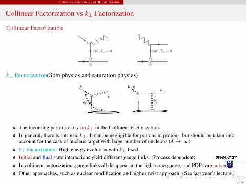
Collinear Factorization vs k⊥ Factorization

Collinear Factorization

xp+, k⊥ = 0 xp+, k⊥ = 0

k⊥ Factorization(Spin physics and saturation physics)

The incoming partons carry no k⊥ in the Collinear Factorization.In general, there is intrinsic k⊥. It can be negligible for partons in protons, but should be taken intoaccount for the case of nucleus target with large number of nucleons (A → ∞).k⊥ Factorization: High energy evolution with k⊥ fixed.Initial and final state interactions yield different gauge links. (Process dependent)In collinear factorization, gauge links all disappear in the light cone gauge, and PDFs are universal.Other approaches, such as nuclear modification and higher twist approach. (See last year’s lecture.)

18 / 56

Collinear Factorization and DGLAP equation Transverse Momentum Dependent (TMD or kt ) Factorization

kt dependent parton distributions

The unintegrated quark distribution

fq(x, k⊥) =

dξ−d2ξ⊥4π(2π)2 e

ixP+ξ−+iξ⊥·k⊥P

ψ(0)L†(0)γ+L(ξ−, ξ⊥)ψ(ξ⊥, ξ

−)P

as compared to the integrated quark distribution

fq(x) =

dξ−

4πe

ixP+ξ−

Pψ(0)γ+

L(ξ−)ψ(0, ξ−)P

The dependence of ξ⊥ in the definition.Gauge invariant definition.Light-cone gauge together with proper boundary condition ⇒ parton densityinterpretation.The gauge links come from the resummation of multiple gluon interactions.Gauge links may vary among different processes.

19 / 56

Collinear Factorization and DGLAP equation Transverse Momentum Dependent (TMD or kt ) Factorization

TMD factorization

One-loop factorization:

For gluon with momentum k

k is collinear to initial quark ⇒ parton distribution function;k is collinear to the final state quark ⇒ fragmentation function.k is soft divergence (sometimes called rapidity divergence) ⇒ Wilson lines (Soft factor) orsmall-x evolution for gluon distribution.Other kinematical region of the radiated gluon contributes tothe NLO (O(αs) correction) hard factor.See new development in Collins’ book.

20 / 56

Introduction to Small-x Physics BFKL evolution and Balitsky-Kovchegov evolution equations

Deep into low-x region of Protons

Gluon splitting functions (P0qq(ξ) and P

0gg(ξ)) have 1/(1 − ξ) singularities.

Partons in the low-x region is dominated by gluons.Resummation of the αs ln 1

x.

21 / 56


Dual Descriptions of Deep Inelastic Scattering

[A. Mueller, 01; Parton Saturation-An Overview]

Bjorken frame Dipole frame

...

Bjorken frameF2(x,Q

2) =

q

e2qx

fq(x,Q

2) + fq(x,Q2).

Dipole frame

F2(x,Q2) =

f

e2f

Q2

4π2αem

1

0dz

d2

x⊥d2y⊥

|ψT (z, r⊥,Q)|2 + |ψL (z, r⊥,Q)|2

× [1 − S (r⊥)] , with r⊥ = x⊥ − y⊥.

Bjorken: the partonic picture of a hadron is manifest. Saturation shows upas a limit on the occupation number of quarks and gluons.Dipole: the partonic picture is no longer manifest. Saturation appears as the unitarity limitfor scattering. Convenient to resum the multiple gluon interactions.

22 / 56


BFKL evolution

[Balitsky, Fadin, Kuraev, Lipatov;74] The infrared sensitivity of Bremsstrahlung favors theemission of small-x gluons:

p

x << 1

kz = xp

kz1 = x1p

kz = xp

x << x1

p p

x << xn

xn << xn−1

x2 << x1

x1 << 1

Probability of emission:

dp ∼ αsNc

dkz

kz

= αsNc

dx

x

In small-x limit and Leading log approximation:

p ∼∞

n=0

αn

sN

n

c

1

x

dxn

xn

· · · 1

x2

dx1

x1∼ exp

αsNc ln

1x

Exponential growth of the amplitude as function of rapidity;

As compared to DGLAP which resums αsNc ln 1x

ln µ2

µ20

.23 / 56


Derivation of BFKL evolution

Dipole model. [Mueller, 94]Consider a Bremsstrahlung emission of soft gluon zg 1,

P+ (1− ξ)P+,−k⊥

ξP+, k⊥

T aij

and use LC gauge = (+ = 0, − = ⊥·k⊥k+

, ±⊥)

M(k⊥) = −2igTa ⊥ · k⊥

k2⊥

q → qg vertex and Energy denominator.Take the limit k

+g → 0.

Similar to the derivation of Pqq(ξ).

24 / 56


The dipole splitting kernal

The Bremsstrahlung amplitude in the coordinate space

x⊥

z⊥

M(x⊥ − z⊥) =

d2

k⊥eik⊥·(x⊥−z⊥)

M(k⊥)

Use

d2k⊥

⊥ · k⊥

k2⊥

eik⊥·b⊥ = 2πi

⊥ · b⊥

b2⊥

,

⇒ M(x⊥ − z⊥) = 4πgTa ⊥ · (x⊥ − z⊥)

(x⊥ − z⊥)2

25 / 56


The dipole splitting kernal

Consider soft gluon emission from a color dipole in the coordinate space (x⊥, y⊥)

x⊥

z⊥

taij ji

i

y⊥

x⊥

z⊥

y⊥

M(x⊥, z⊥, y⊥) = 4πgTa

⊥ · (x⊥ − z⊥)(x⊥ − z⊥)2 −

⊥ · (y⊥ − z⊥)(y⊥ − z⊥)2

⇒

x⊥z⊥y⊥

= αsNc2π2

(x⊥−y⊥)2

(x⊥−z⊥)2(y⊥−z⊥)

2=

The probability of dipole splitting at large Nc limit

dPsplitting =αsNc

2π2(x⊥ − y⊥)

2

(x⊥ − z⊥)2(x⊥ − z⊥)2 d2z⊥dY with dY =

dk+g

k+g

Gluon splitting ⇔ Dipole splitting.26 / 56


BFKL evolution in Mueller’s dipole model

[Mueller; 94] In large Nc limit, BFKL evolution can be viewed as dipole branching in a fastmoving qq dipole in coordinate space:

Y0 Y1 YY2<<<< <<

n(r, Y) dipoles of size r. BFKL PomeronThe T matrix (T ≡ 1 − S with S being the scattering matrix) basically just counts the number ofdipoles of a given size,

T(r, Y) ∼ α2s n(r, Y)

The probability of emission is αs

(x−y)2

(x−z)2(z−y)2 ;

Assume independent emissions with large separation in rapidity.27 / 56


BFKL equation

Consider a slight change in rapidity and the Bremsstrahlung emission of soft gluon (dipolesplitting)

∂Y =

x

y

z

∂Y T(x, y; Y) =αs

2π

d

2z

(x − y)2

(x − z)2(z − y)2 [T(x, z; Y) + T(z, y; Y)− T(x, y; Y)]

28 / 56


Kovchegov equation

[Kovchegov; 99] [Mueller; 01] Including non-linear effects: (T ≡ 1 − S)

∂S∂Y =

x

y

z

x

z

y

∂Y S(x − y; Y) =αNc

2π2

d

2z

(x − y)2

(x − z)2(z − y)2 [S(x − z; Y)S(z − y; Y)− S(x − y; Y)]

∂Y T(x − y; Y) =αNc

2π2

d

2z

(x − y)2

(x − z)2(z − y)2

×

T(x − z; Y) + T(z − y; Y)− T(x − y; Y)− T(x − z; Y)T(z − y; Y)

saturation

Linear BFKL evolution results in fast energy evolution.

Non-linear term ⇒ fixed point (T = 1) and unitarization, and thus saturation.29 / 56


Phase diagram in QCD

Low Q2 and low x region ⇒ saturation region.

Balitsky-Kovchegov equation is the non-linear small-x evolution equationwhich describes the saturation physics.

30 / 56


Balitsky-Kovchegov equation vs F-KPP equation

[Munier, Peschanski, 03] Consider the case with fixed impact parameter, namely, Txy is onlyfunction of r = x − y. Then, transforming the B-K equation into momentum space:

BK equation: ∂Y T = αχBFKL(−∂ρ)T − αT2 with α =

αNc

πDiffusion approximation ⇒

F-KPP equation: ∂tu(x, t) = ∂2x u(x, t) + u(x, t)− u

2(x, t)

u ⇒ T , αY ⇒ t, = log(k2/k20) ⇒ x, with k0 being the reference scale;

B-K equation lies in the same universality class as the F-KPP[Fisher-Kolmogrov-Petrovsky-Piscounov; 1937] equation.F-KPP equation admits traveling wave solution u = u (x − vt) with minimum velocity;the non-linear term saturates the solution in the infrared.

31 / 56


Balitsky-Kovchegov equation vs F-KPP equation

BK equation: ∂Y T = αχBFKL(−∂)T − αT2

The linear part of its solution Tlin(k, Y) is asuperposition of waves:

Tlin(k, Y) =

c+i∞

c−i∞

dγ2iπ

exp [−γ (− αv(γ)Y)] T0(γ)γc

γ

χ(γ)/γ

10.80.60.40.20

8

7

6

5

4

3

2

1

0

T0(γ): the initial condition,

Each wave has a different speed v(γ) given by v(γ) = χ(γ)γ with

χ(γ) = ψ(1)− 12ψ(γ)−

12ψ(1 − γ) and ψ(γ) = d

dγ log[Γ(γ)] being the digammafunction.[Mueller, Triantafyllopoulos; 02]Using saddle point approximation, and requiringexponent vanishes at the saddle point. one gets γc = 0.63. This corresponds to ananomalous dimension 0.37.The wave speed v(γ) is minimized at γc = 0.63. γc is selected by exponential growth andsaturation.

32 / 56


Geometrical scaling

Geometrical scaling in DIS:

T (r, Y) = T

r

2Q

2s (Y)

=r

2Q

2s (Y)

γc

exp

−

log2 r

2Q

2s (Y)

2χ (γc) αY

Scaling window

All data of σγ∗p

tot when x ≤ 0.01 and 1r2 = Q

2≤ 450GeV

2 plotting as function ofτ = Q

2/Q2s falls on a curve, where Q

2s =

x0x

0.29GeV

2 with x0 = 3 × 10−4;scaling window: | log

r

2Q

2s (Y)

|

2χ (γc) αY .

γ∗γ∗

p,Ap,A

[Golec-Biernat, Stasto, Kwiecinski; 01]33 / 56

Introduction to Small-x Physics McLerran-Venugopalan Model

McLerran-Venugopalan Model

In QCD, the McLerran-Venugopalan Model describes high density gluon distribution in arelativistic large nucleus (A 1) by solving the classical Yang-Mills equation:

[Dµ,Fµν ] = gJ

ν with Jν = δν+ρa(x

−, x⊥)Ta, COV gauge ⇒ −

2⊥ A

+ = gρ.

To solve the above equation, we define the Green’s function

2z⊥G(x⊥ − z⊥) = δ(2)(x⊥ − z⊥) ⇒ G(x⊥ − z⊥) = −

d2

k⊥

(2π)2e

ik⊥·(x⊥−z⊥)

k2⊥

MV model assumes that the density of color charges follows a Gaussian distribution

W[ρ] = exp−

dz

−d2z⊥

ρa(z−, z⊥)ρa(z

−, z⊥)2µ2(z−)

.

With such a weight, average of two color sources is

ρaρb =

D[ρ]W[ρ]ρa(x

−, x⊥)ρb(y−, y⊥) = µ2(x−)δabδ(x

−− y

−)δ(x⊥ − y⊥).

34 / 56


Dipole amplitude in MV model

The Wilson line [F. Gelis, A. Peshier, 01]

U(x⊥) = P exp−ig

2

dz−d2

z⊥G (x⊥ − z⊥) ρz−, z⊥

· · ·U(x⊥) ≡ · · ·

x⊥y⊥

x⊥S(x⊥, y⊥) ≡ 1

NcTrU(x⊥)U †(y⊥)

Use gaussian approximation to pair color charges:

z -1 z -2 z -1 z -2 z -3 z -4 z -5 z -6

⇒ S(x⊥, y⊥) exp−µ2

s

4

d2

z⊥ [G (x⊥ − z⊥)− G (y⊥ − z⊥)]2

exp− 1

4Q

2s(x⊥ − y⊥)2

⇐ GBW model

Quadrupoles 1Nc

TrU1U†2 U3U

†4 and Sextupoles 1

NcTrU1U

†2 U3U

†4 U5U

†6 ...

35 / 56


Golec-Biernat Wusthoff model and Geometrical Scaling

[Golec-Biernat, Wusthoff,; 98], [Golec-Biernat, Stasto, Kwiecinski; 01]

W=245 (x128)

W=210 (x64)

W=170 (x32)

W=140 (x16)

W=115 (x8)

W=95 (x4)

W=75 (x2)

W=60 (x1)

Q2 (GeV2)

*p (!

b)

Q2 (GeV2)

*p (!

b)

1

10

10 2

10 3

10 4

10-2

10-1

1 10 102 10

-1

1

10

10 2

10 3

10 -3 10 -2 10 -1 1 10 10 2 10 3

E665ZEUS+H1 high Q2 94-95H1 low Q2 95ZEUS BPC 95ZEUS BPT 97

x<0.01

all Q2

tot

*p [µ

b]

The dipole amplitude in the GBW model

Sqq(r⊥) = exp[−Q

2s r

2⊥

4]

with Q2s (x) = Q

2s0(x0/x)λ where Qs0 = 1GeV, x = 3.04 × 10−3 and λ = 0.288.

36 / 56

Dihadron Correlations Breaking down of the kt factorization in di-jet production

Kt Factorization "expectation"

Consider the inclusive production of two high-transverse-momentum back-to-back particles inhadron-hadron collisions, i.e., in the process:

H1 + H2 → H3 + H4 + X.

p1 p2

Jet 1

Jet 2

k2

k1

k3

k4

The standard kt factorization "expectation" is:

E3E4dσ

d3p3d3

p4=

dσi+j→k+l+Xfi/1fj/2d3/kd4/l+ · · ·

Convolution of dσ with f (x, k⊥) and d(z).Factorization ⇔ Factorization formula + UniversalityOnly Drell-Yan process is proved for factorization in hadron-hadroncollisions. [Bodwin; 85, 86], [Collins, Soper, Sterman; 85, 88].

37 / 56


Breaking down of the kt factorization in di-hadron production

[Bacchetta, Bomhof, Mulders and Pijlman; 04-06] Wilson lines approachStudies of Wilson-line operators show that the TMD parton distributions are not generallyprocess-independent due to the complicated combinantion of initial and final state interactions. TMDPDFs admit process dependent Wilson lines.

[Collins, Qiu; 07], [Collins; 07], [Vogelsang, Yuan; 07] and [Rogers, Mulders; 10]Scalar QED models and its generalization to QCD (Counterexample to Factorization)

O(g2) calculation shows non-vanishing anomalous terms with respect to standard factorization.

Remarks: kt factorization is violated in di-jet production; TMD parton distributions are non-universal.

Things get worse: For pp and AA collisions, no factorization formula at all for dijet production.

38 / 56


Why is the di-jet production process special?

Initial state interactions and/or final state interactions

In Drell-Yan process, there are only initial state interactions. +∞

−∞dk

+g

i

−k+g − i

A+(kg) =

−∞

0dζ−A

+(ζ−)

Eikonal approximation =⇒ gauge links.In DIS, there are only final state interactions.

+∞

−∞dk

+g

i

−k+g + i

A+(kg) =

+∞

0dζ−A

+(ζ−)

Eikonal approximation =⇒ gauge links.However, there are both initial state interactions and final state interactions inthe di-jet process.

39 / 56

Dihadron Correlations Probing two fundamental gluon distributions

Forward observables at pA collisions

Why pA collisions?For pA (dilute-dense system) collisions, there is an effective kt factorization.

dσpA→qfX

d2P⊥d2q⊥dy1dy2=xpq(xp, µ

2)xAf (xA, q2⊥)

1π

dσdt

.

For dijet processes in pp, AA collisions, there is no kt factorization[Collins, Qiu,08],[Rogers, Mulders; 10].

Why forward?At forward rapidity y, xp ∝ e

y is large, while xA ∝ e−y is small.

Ideal place to find gluon saturation in the target nucleus.40 / 56


A Tale of Two Gluon Distributions

In small-x physics, two gluon distributions are widely used:[Kharzeev, Kovchegov, Tuchin; 03]I. Weizsacker Williams gluon distribution ([KM, 98’] and MV model):

xG(1) =

S⊥

π2αs

N2c − 1Nc

⇐

×

d

2r⊥

(2π)2e−ik⊥·r⊥

r2⊥

1 − e

−r2⊥Q

2sg

2

II. Color Dipole gluon distributions:

xG(2) =

S⊥Nc

2π2αs

k2⊥ ⇐

×

d

2r⊥

(2π)2 e−ik⊥·r⊥e

−r2⊥Q

2sq

4

rT

Remarks:The WW gluon distribution simply counts the number of gluons.The Color Dipole gluon distribution often appears in calculations.Does this mean that gluon distributions are non-universal? Answer: Yes and No!

41 / 56



[F. Dominguez, C. Marquet, BX and F. Yuan, 11]I. Weizsacker Williams gluon distribution

xG(1) =

S⊥

π2αs

N2c − 1Nc

⇐

×

d

2r⊥

(2π)2e−ik⊥·r⊥

r2⊥

1 − e

−r2⊥Q

2s

2


xG(2) =

S⊥Nc

2π2αs

⇐

×

d

2r⊥

(2π)2 e−ik⊥·r⊥∇

2r⊥N(r⊥)

0.0 0.5 1.0 1.5 2.0 2.5 3.00.00

0.05

0.10

0.15

0.20

0.25

q2

Qs2

xGx,q

A tale of two gluon distributions

42 / 56



In terms of operators (known from TMD factorization), we find these two gluon distributionscan be defined as follows: [F. Dominguez, C. Marquet, BX and F. Yuan, 11]I. Weizsacker Williams gluon distribution:

xG(1) = 2

dξ−dξ⊥(2π)3P+

eixP

+ξ−−ik⊥·ξ⊥TrP|F+i(ξ−, ξ⊥)U[+]†

F+i(0)U [+]

|P.


xG(2) = 2


eixP

+ξ−−ik⊥·ξ⊥TrP|F+i(ξ−, ξ⊥)U[−]†

F+i(0)U [+]

|P.

T T

U[−]

U[+]

Remarks:The WW gluon distribution is the conventional gluon distributions. In light-cone gauge, itis the gluon density. (Only final state interactions.)The dipole gluon distribution has no such interpretation. (Initial and final stateinteractions.)Both definitions are gauge invariant.Same after integrating over q⊥.Same perturbative tail.

43 / 56



In terms of operators, we find these two gluon distributions can be defined as follows: [F.Dominguez, C. Marquet, BX and F. Yuan, 11]I. Weizsacker Williams gluon distribution:

xG(1) = 2


eixP

+ξ−−ik⊥·ξ⊥TrP|F+i(ξ−, ξ⊥)U[+]†

F+i(0)U [+]

|P.


xG(2) = 2


eixP

+ξ−−ik⊥·ξ⊥TrP|F+i(ξ−, ξ⊥)U[−]†

F+i(0)U [+]

|P.

T T

U[−]

U[+]

Questions:Can we distinguish these two gluon distributions? Yes, We Can.How to measure xG

(1) directly? DIS dijet.How to measure xG

(2) directly? Direct γ+Jet in pA collisions.For single-inclusive particle production in pA up to all order.What happens in gluon+jet production in pA collisions? It’s complicated!

44 / 56


DIS dijet

[F. Dominguez, C. Marquet, BX and F. Yuan, 11]

(a) (b) (c)

q2 q2

k1

k2 k2

k1

dσγ∗T

A→qq+X

dP.S.∝ Ncαeme

2q

d2

x

(2π)2d2

x

(2π)2d2

b

(2π)2d2

b

(2π)2 e−ik1⊥·(x−x

)

×e−ik2⊥·(b−b

)

ψ∗T (x − b)ψT(x

− b

)1 + S

(4)xg

(x, b; b, x

)− S(2)xg

(x, b)− S(2)xg

(b, x)

−uiu

j

1Nc

Tr[∂iU(v)]U†(v)[∂jU(v)]U†(v)xg⇒Operator Def

,

Eikonal approximation ⇒ Wilson Line approach [Kovner, Wiedemann, 01].In the dijet correlation limit, where u = x − b v = zx + (1 − z)b

S(4)xg

(x, b; b, x

) = 1Nc

TrU(x)U†(x)U(b)U†(b)

xg

= S(2)xg

(x, b)S(2)xg

(b, x)

Quadrupoles are generically different objects and only appear in dijet processes.45 / 56


DIS dijet

The dijet production in DIS.

(a) (b) (c)

q2 q2

k1

k2 k2

k1

TMD factorization approach:

dσγ∗T

A→qq+X

dP.S.= δ(xγ∗ − 1)xgG

(1)(xg, q⊥)Hγ∗T

g→qq,

Remarks:Dijet in DIS is the only physical process which can measure Weizsacker Williams gluondistributions.Golden measurement for the Weizsacker Williams gluon distributions of nuclei at small-x.The cross section is directly related to the WW gluon distribution.EIC and LHeC will provide us a perfect machine to study the stronggluon fields in nuclei. Important part in EIC and LHeC physics.

46 / 56


γ+Jet in pA collisions

The direct photon + jet production in pA collisions. (Drell-Yan follows the same factorization.)TMD factorization approach:

dσ(pA→γq+X)

dP.S.=

f

x1q(x1, µ2)xgG

(2)(xg, q⊥)Hqg→γq.

Remarks:Independent CGC calculation gives the identical result in the correlation limit.Direct measurement of the Color Dipole gluon distribution.

47 / 56


DY correlations in pA collisions

[Stasto, BX, Zaslavsky, 12]

0 π2

π 3π2

2π0

0.002

0.004σDYF/σ

DYSIF

GBWBKrcBK

0 π2

π 3π2

2π0

0.001

0.002

0.003

∆φ

σDYF/σ

DYSIF

GBWBKrcBK

0 π2

π 3π2

2π0

0.01

0.02

0.03

σDYF/σ

DYSIF

GBWBKrcBK

0 π2

π 3π2

2π0

0.01

0.02

0.03

0.04

∆φ

σDYF/σ

DYSIF

GBWBKrcBK

M = 0.5, 4GeV, Y = 2.5 at RHIC dAu. M = 4, 8GeV, Y = 4 at LHC pPb.Partonic cross section vanishes at π ⇒ Dip at π.Prompt photon calculation [J. Jalilian-Marian, A. Rezaeian, 12]

48 / 56

Dihadron Correlations Gluon+Jet in pA

STAR measurement on di-hadron correlation in dA collisions

There is no sign of suppression in the p + p and d + Au peripheral data.The suppression and broadening of the away side jet in d + Au central collisions is due tothe multiple interactions between partons and dense nuclear matter (CGC).Probably the best evidence for saturation.

49 / 56


First calculations on dijet production

Quark+Gluon channel [Marquet, 07] and [Albacete, Marquet, 10]

p q

k

p q

k

!"0 1 2 3 4 5 6

)

!"

CP(

0

0.005

0.01

0.015

0.02 STAR PRELIMINARY>2 GeV/cT,L

p

T,L<p

T,S1 GeV/c < p p+p (−0.0045)

d+Au central (−0.0145)

Prediction of saturation physics.All the framework is correct, but over-simplified 4-point function.Improvement [F. Dominguez, C. Marquet, BX and F. Yuan, 11.]

S(4)xg

(x1, x2; x2, x

1) e

− CF

2 [Γ(x1−x2)+Γ(x2−x

1)]

−F(x1, x2; x

2, x

1)

F(x1, x2; x2, x

1)

e− CF

2 [Γ(x1−x2)+Γ(x2−x

1)] − e

− CF

2 [Γ(x1−x1)+Γ(x

2−x2)]

50 / 56


Dijet processes in the large Nc limit

The Fierz identity:

= 12

− 12Nc and

= 12

−12

Graphical representation of dijet processesg → qq:

!"

!#

!$"

!$#%&'!#()# '*!" %$&'!$#()# '*!$"

⇒

= 12

− 12Nc

q → qg

!

"

!#

"#

$%&"'() &*! $#%&"#'() &*!#

⇒

2= = 1

2− 1

2Nc

g → gg

!" !#"$%&!"'(" &)!* $#%&!#"'(" &)!#*

!* !#*

⇒

= −

= −

The Octupole and the Sextupole are suppressed.51 / 56


Gluon+quark jets correlation

Including all the qg → qg, gg → gg and gg → qq channels, a lengthy calculation gives

dσ(pA→Dijet+X)

dP.S.=

q

x1q(x1, µ2)

α2s

s2

F(1)

qg H(1)qg + F(2)

qg H(2)qg

+x1g(x1, µ2)

α2s

s2

F(1)

gg

H

(1)gg→qq

+12

H(1)gg→gg

+F(2)gg

H

(2)gg→qq

+12

H(2)gg→gg

+ F(3)

gg

12

H(3)gg→gg

,

with the various gluon distributions defined as

F(1)qg = xG

(2)(x, q⊥), F(2)qg =

xG

(1) ⊗ F ,

F(1)gg =

xG

(2) ⊗ F, F(2)gg = −

q1⊥ · q2⊥

q21⊥

xG(2) ⊗ F ,

F(3)gg =

xG

(1)(q1)⊗ F ⊗ F ,

where F =

d2r⊥

(2π)2 e−iq⊥·r⊥ 1

Nc

TrU(r⊥)U†(0)

xg

.Remarks:

Only the term in NavyBlue color was known before.

This describes the dihadron correlation data measured at RHIC in forward dAu collisions.52 / 56


Illustration of gluon distributions

The various gluon distributions:

xG(1)WW(x, q⊥), F

(1)qg = xG

(2)(x, q⊥),

F(1)gg =

xG

(2)⊗ F, F

(2)gg = −

q1⊥ · q2⊥

q21⊥

xG(2)

⊗ F ,

F(3)gg =

xG

(1)(q1)⊗ F ⊗ F , F(2)qg =

xG

(1)⊗ F

0 1 2 3 4

0.00

0.05

0.10

0.15

0.20

q2

Qs2

xGx,q

6 different gluon distributions

53 / 56


Comparing to STAR and PHENIX data

Physics predicted by C. Marquet. Further calculated in[A. Stasto, BX, F. Yuan, 11]

Forward di-hadron correlations in

d+Au collisions at RHIC

!"=0

(near side)!"=#

(away side)

(rad)

! “Coincidence probability” at measured by STAR Coll. at forward rapidities:

CP (∆φ) =1

Ntrig

dNpair

d∆φ∆φ

trigger

! Absence of away particle in d+Au coll.

“monojets”! Away peak is present in p+p coll.

d+Au central

p+p

trigger

associated

(k1, y1)(k2, y2) xA =

|k1| e−y1 + |k2| e−y2

√s

20

For away side peak in both peripheral and central dAu collisions

C(∆φ) =

|p1⊥|,|p2⊥|

dσpA→h1h2

dy1dy2d2p1⊥d2p2⊥|p1⊥|

dσpA→h1dy1d2p1⊥

JdA =1

Ncoll

σpairdA

/σdA

σpairpp /σpp

-310 -210

-110

1

peripheral

central

fragAux

dAuJ

Using: Q2sA = c(b)A1/3

Q2s (x).

Physical picture: Dense gluonic matter suppresses the away side peak.54 / 56


Conclusion and Outlook

Conclusion:DIS dijet provides direct information of the WW gluon distributions. Perfect for testingCGC, and ideal measurement for EIC and LHeC.Modified Universality for Gluon Distributions:

Inclusive Single Inc DIS dijet γ +jet g+jetxG

(1)× ×

√×

√

xG(2), F

√ √×

√ √

× ⇒ Do Not Appear.√

⇒ Apppear.Two fundamental gluon distributions. Other gluon distributions are just differentcombinations and convolutions of these two.The small-x evolution of the WW gluon distribution, a different equation fromBalitsky-Kovchegov equation;[Dominguez, Mueller, Munier, Xiao, 11]Dihadron correlation calculation agrees with the RHIC STAR and PHENIX data.

55 / 56


Outlook

[Dominguez, Marquet, Stasto, BX, in preparation] Use Fierz identity:

= 12

− 12Nc

The three-jet (same rapidity) production processes in the large Nc limit:

qqg-jet

2

= = 12

− 12Nc

In the large Nc limit at small-x, the dipole and quadrupole amplitudes are the only twofundamental objects in the cross section of multiple-jet production processes at any orderin terms αs.Other higher point functions, such as sextupoles, octupoles, decapoles and duodecapoles,etc. are suppressed by factors of 1

N2c

.

56 / 56

introduction to qcd and jet ii

Documents