introduction to programming econometrics with...

Introduction to programmingEconometrics with R

Bruno RodriguesUniversity of Strasbourg

FSEG, Beta-CNRShttp://www.brodrigues.co

1st edition, 2014

This work, including its figures, LATEXand accompanying R source code, is licensed under theCreative Commons Attribution-NonCommercial-ShareAlike 4.0 International License. To view acopy of this license, visit http://creativecommons.org/licenses/by-nc-sa/4.0/legalcode

Get the book’s source code here: https://bitbucket.org/b-rodrigues/programmingeconometrics

http://creativecommons.org/licenses/by-nc-sa/4.0/legalcode

https://bitbucket.org/b-rodrigues/programmingeconometrics

Preface

This book is primarily intended for third year students of the Quantitative Economics section atthe faculty of economics from the University of Strasbourg, France. The goal is to teach themthe basics of programming with R, and applying this knowledge to solve problems in economics,finance and marketing. You are free to redistribute free copies of this book. You are also free tomodify, remix, transform or adapt the contents of this book, but please, give appropriate credit ifyou do use this book.

Contents

1 A short history of R, installation instructions and asking for help 61.1 History of R: Bell Labs’ ”S” . . . . . . . . . . . . . . . . . . . . . . . . . . . . . . . 61.2 Why use R? Why not Excel? . . . . . . . . . . . . . . . . . . . . . . . . . . . . . . 61.3 Installation . . . . . . . . . . . . . . . . . . . . . . . . . . . . . . . . . . . . . . . . 7

1.3.1 Windows . . . . . . . . . . . . . . . . . . . . . . . . . . . . . . . . . . . . . 71.3.2 Linux . . . . . . . . . . . . . . . . . . . . . . . . . . . . . . . . . . . . . . . 71.3.3 OSX . . . . . . . . . . . . . . . . . . . . . . . . . . . . . . . . . . . . . . . . 71.3.4 Other versions of R . . . . . . . . . . . . . . . . . . . . . . . . . . . . . . . 7

1.4 How to ask for help . . . . . . . . . . . . . . . . . . . . . . . . . . . . . . . . . . . . 81.4.1 Mailing lists, chat rooms and forums . . . . . . . . . . . . . . . . . . . . . . 8

2 R basics 92.1 Vocabulary . . . . . . . . . . . . . . . . . . . . . . . . . . . . . . . . . . . . . . . . 92.2 Style Guidelines . . . . . . . . . . . . . . . . . . . . . . . . . . . . . . . . . . . . . . 102.3 Data types and objects . . . . . . . . . . . . . . . . . . . . . . . . . . . . . . . . . . 10

2.3.1 Integers . . . . . . . . . . . . . . . . . . . . . . . . . . . . . . . . . . . . . . 102.3.2 Floating point numbers . . . . . . . . . . . . . . . . . . . . . . . . . . . . . 112.3.3 Strings . . . . . . . . . . . . . . . . . . . . . . . . . . . . . . . . . . . . . . . 112.3.4 Vectors and matrices . . . . . . . . . . . . . . . . . . . . . . . . . . . . . . . 112.3.5 The c command . . . . . . . . . . . . . . . . . . . . . . . . . . . . . . . . . 112.3.6 The cbind command (and rbind also) . . . . . . . . . . . . . . . . . . . . . 122.3.7 The Matrix class . . . . . . . . . . . . . . . . . . . . . . . . . . . . . . . . . 122.3.8 The logical class . . . . . . . . . . . . . . . . . . . . . . . . . . . . . . . . . 13

2.4 Control Flow . . . . . . . . . . . . . . . . . . . . . . . . . . . . . . . . . . . . . . . 152.4.1 If-else . . . . . . . . . . . . . . . . . . . . . . . . . . . . . . . . . . . . . . . 152.4.2 For loops . . . . . . . . . . . . . . . . . . . . . . . . . . . . . . . . . . . . . 172.4.3 While loops . . . . . . . . . . . . . . . . . . . . . . . . . . . . . . . . . . . . 17

2.5 Functions . . . . . . . . . . . . . . . . . . . . . . . . . . . . . . . . . . . . . . . . . 192.5.1 Declaring functions in R . . . . . . . . . . . . . . . . . . . . . . . . . . . . . 192.5.2 Fibonacci numbers . . . . . . . . . . . . . . . . . . . . . . . . . . . . . . . . 19

2.6 Preprogrammed functions available in R . . . . . . . . . . . . . . . . . . . . . . . . 212.6.1 Numeric functions . . . . . . . . . . . . . . . . . . . . . . . . . . . . . . . . 212.6.2 Statistical and probability functions . . . . . . . . . . . . . . . . . . . . . . 222.6.3 Matrix manipulation . . . . . . . . . . . . . . . . . . . . . . . . . . . . . . . 222.6.4 Other useful commands . . . . . . . . . . . . . . . . . . . . . . . . . . . . . 23

2.7 Putting it all together . . . . . . . . . . . . . . . . . . . . . . . . . . . . . . . . . . 232.7.1 Maximum Likelihood estimation . . . . . . . . . . . . . . . . . . . . . . . . 23

3 Applied econometrics with R 273.1 Importing data . . . . . . . . . . . . . . . . . . . . . . . . . . . . . . . . . . . . . . 27

3.1.1 A small digression: packages . . . . . . . . . . . . . . . . . . . . . . . . . . 283.1.2 Back to importing data . . . . . . . . . . . . . . . . . . . . . . . . . . . . . 30

3.2 One last data type: the data frame type . . . . . . . . . . . . . . . . . . . . . . . . 313.3 Summary statistics . . . . . . . . . . . . . . . . . . . . . . . . . . . . . . . . . . . . 31

4

0 Introduction to programming Econometrics with R

3.3.1 Conditional summary statistics . . . . . . . . . . . . . . . . . . . . . . . . . 323.3.2 Getting descriptive statistics easier with dplyr . . . . . . . . . . . . . . . . 33

3.4 Plots . . . . . . . . . . . . . . . . . . . . . . . . . . . . . . . . . . . . . . . . . . . . 343.4.1 Histograms . . . . . . . . . . . . . . . . . . . . . . . . . . . . . . . . . . . . 343.4.2 Scatter plots and line graphs . . . . . . . . . . . . . . . . . . . . . . . . . . 37

3.5 Linear Models . . . . . . . . . . . . . . . . . . . . . . . . . . . . . . . . . . . . . . . 42

4 Reproducible research 474.1 What is reproducible research? . . . . . . . . . . . . . . . . . . . . . . . . . . . . . 474.2 Using R and Rstudio for reproducible research . . . . . . . . . . . . . . . . . . . . 47

CONTENTS 5

Chapter 1

A short history of R, installationinstructions and asking for help

1.1 History of R: Bell Labs’ ”S”

R is a modern implementation of the S language. S was developed at Bell Labs where the UNIXoperating system, the C language as well as the C++ language were developed. As such R and Sare very similar, but R is much more widely used, in part due to its free license, the GPL. The GPLallows users to freely share their own modifications of the software, thus allowing the widespreaduse of R worldwide.

R is an interpreted language, making it very easy to use: you don’t need to compile the code toget the results of your analysis. A lot of pre-programmed routines are included, and you can addmore through packages. As such, you can use R in two ways, as S’s creator suggests:

” [W]e wanted users to be able to begin in an interactive environment, where theydid not consciously think of themselves as programming. Then as their needs becameclearer and their sophistication increased, they should be able to slide gradually intoprogramming, when the language and system aspects would become more important.”

John Chambers, the creator of S, in Stages in the Evolution of S.

The main idea behind this quote, is that you could use S without knowing a lot about programmingor the language itself. However, when your needs would grow, you could go beyond using simplebuilt-in commands, and program your own. This is possible with R of course, and this book willfocus on programming your own functions and routines to solve economic, financial, and marketingproblems.

1.2 Why use R? Why not Excel?

R and Excel are very different tools, for very different purposes. Just like you wouldn’t use ahammer to cut bread, you shouldn’t use Excel (or similar software) to do econometrics. R, andother programming languages, make it very easy to go far beyond the pre-programmed routines.R has also other advantages, such as:

1. Runs on any modern operating system

2. Very rapid and active development. There are yearly releases, and minor releases in betweento fix bugs

3. Very nice graphs (especially with ggplot2, a package that makes beautiful graphs)

6


4. Huge user community, getting help is easy

5. R is free software; which means

• No vendor-lockin

• Free to download

All this makes R a very attractive alternative to other data analysis tools like Excel, STATA or SAS.So much so that R is, according to the TIOBE index1, the most popular programming languagefor data analysis. In December 2014, R was the 12th most popular programming language. All theother languages in front of R were general purpose languages. MATLAB was at the 20th positionand SAS at the 21st. R is not only used in academia for teaching purposes, but is also used by Bankof America, Bing, Facebook, Ford, Google, Kickstarter, Mozilla, The New York Times, Twitter,Uber2 and much more.

1.3 Installation

This section contains installation instructions for Windows, OSX and some Linux distributions.We will install two things: R itself, and Rstudio, an IDE for R. An IDE (Integrated DevelopmentEnvironment) is an interface that allows the user to program more efficiently. There are other IDEavailable for R, but Rstudio is probably the best one.

1.3.1 Windows

Go to the following url http://cran.r-project.org/bin/windows/base/ and download the lat-est version of R. Since you’re probably using a modern computer, install the 64-bit version. Oncethe installation is complete, you can download Rstudio here: http://www.rstudio.com/ide/

download/desktop. Install Rstudio, and you’re done.

1.3.2 Linux

For Debian-based systems, run the following command in a terminal: sudo apt-get install

r-base. Once the installation is complete, you can download Rstudio here: http://www.rstudio.com/ide/download/desktop.

1.3.3 OSX

You can find R at the following http://cran.r-project.org/bin/macosx/. For Rstudio, followthe instructions above.

1.3.4 Other versions of R

There are other versions of R available that you can install. The most interesting one is probablyRevolution R Open. You can get this version here: http://mran.revolutionanalytics.com/

download/. This version is made by Revolution Analytics and is fully compatible with the tra-ditional version of R, but is much, much faster. For our purposes though, good old R is enough.But if sometime down the road you need more speed, Revolution R Open is a very good option.

1http://www.tiobe.com/index.php/content/paperinfo/tpci/index.html2http://www.revolutionanalytics.com/companies-using-r

CHAPTER 1. A SHORT HISTORY OF R, INSTALLATION INSTRUCTIONS AND ASKINGFOR HELP

7

http://cran.r-project.org/bin/windows/base/

http://www.rstudio.com/ide/download/desktop




http://cran.r-project.org/bin/macosx/

http://mran.revolutionanalytics.com/download/

http://mran.revolutionanalytics.com/download/

http://www.tiobe.com/index.php/content/paperinfo/tpci/index.html

http://www.revolutionanalytics.com/companies-using-r


1.4 How to ask for help

1.4.1 Mailing lists, chat rooms and forums

Something very important you need to learn very early on when you start programming: how toask for help. Let’s make something clear; this is probably the most important skill that you’llneed. 90% of programming is googling for solutions to your problems, copy/paste code and thenadapt it to your problem. As you get more experience, you will be able to do a lot yourself butthere will always be something that you will not know how to do. Asking for help, and knowinghow to ask for help is crucial.

Before asking for help, you should consult R’s built-in help. For example, to get information ofthe lm() function, you would type:

> options(continue="

+ ")

> help(lm)

At the end of the help file, examples are often given. If after reading the help file you still havetrouble, try to read the error messages and understand them. For instance, the following command:

> lm(y~x)

could return the following error: Error in eval(expr, envir, enclos) : object ’y’ not

found and you need to understand what this means: here, you tried to run a linear regressionwithout telling R what the variable y is. Do not forget that R only does what you ask him to, andthat it can’t read your mind. If you are really at a loss, you can ask for help in the official mailinglist. Here is the guide to post in the mailing list http://www.r-project.org/posting-guide.

html. You can also ask for help on irc. Go to http://webchat.freenode.net/, enter a nicknameand put ”#r” as the channel you want to connect to. You’ll enter a chat room dedicated to helpR users. You can also ask for at stackoverflow3. This is a website dedicated to programming ingeneral, so you will have to specify that you have trouble with R.

Another piece of advice: you should type every command you read here in this book and try themfor yourself. It is the best way to learn.

Now that you know all this, I suggest you watch this video I made that shows you how to useRstudio: https://copy.com/HoLU9eqjB6eK9Qhr. The video uses the .mp4 format, and works onFirefox and Chrome.

Exercises

Exercise 1 After having installed R and Rstudio, launch Rstudio and run the following command:R.Version(). Email me the output in a .txt at [email protected].

3https://stackoverflow.com/

CHAPTER 1. A SHORT HISTORY OF R, INSTALLATION INSTRUCTIONS AND ASKINGFOR HELP

8

http://www.r-project.org/posting-guide.html

http://www.r-project.org/posting-guide.html

http://webchat.freenode.net/

https://copy.com/HoLU9eqjB6eK9Qhr

https://stackoverflow.com/

Chapter 2

R basics

In this chapter, we will learn some basic vocabulary. Knowing how things are called makes it easierfor you to ask for help and also get help. Most definitions are taken from Wikipedia.

2.1 Vocabulary

• Programming language: a formal constructed language designed to communicate instructionsto a computer. R is a programming language dedicated to statistics and econometrics.

• Source code: the source code is the file in which you write the instructions. In R, these fileshave a .R extension. So for example, for you would save the instructions to complete exercise1 in a file called ex1.R.

• Command prompt: In Rstudio, you have a pane where you write your script, and anotherpane that is the command prompt. You can write commands directly in the commandprompt, and the results are shown in the command prompt.

9


• Object: in a programming language, an object is a location in memory with a value and anidentifier. An object can be a variable, a data structure (such as a matrix) or a function. Anobject has generally a type or a class.

• Class: determines the nature of an object. For example, if A is a matrix, then A would beof class matrix.

• Identifier: the name of an object. In the example above, A is the identifier.

• Comments: in your script file, you can also add comments. Comments begin with a # symboland are not executed by R.

2.2 Style Guidelines

These guidelines ensure that you write nice code that everyone can understand. These are allshamelessly taken from Google’s R Style Guide.1 For more details and examples, read the wholeguide online.

• File names should end in .R

• Identifiers for numbers and vectors should be written in lowercase. For matrices in uppercase.Function names should use the CapsWords convention.

• Indentation: two spaces.

• Spacing: put spaces around all operators =, +, -, <-, etc..

• Curly braces: first on same line, last on own line.

• Comments: after the # symbol, add a space.

• Constants: constants are defined only with uppercase letters.Example, say you want to definea constant: α = 3, define it like this: ALPHA = 3.

2.3 Data types and objects

R use a variety of data types. You already know most of them, actually! Integers (nombres entiers),floating point numbers, or floats (nombres reels), matrices, etc, are all objects you already use ona daily basis. But R has a lot of other data types (that you can find in a lot of other programminglanguages) that you need to become familiar with.

2.3.1 Integers

Integers are numbers that can be written without a fractional or decimal component, such as 2,-78, 1024, etc. You can assign an integer to a variable of your choice. For instance:

> p <- as.integer(3)

The above code means: ”put the integer 3 in a variable called p”. The <- is very important; it’sthe assignment operator. You can check if p is an integer with the class command:

> class(p)

[1] "integer"

1https://google-styleguide.googlecode.com/svn/trunk/Rguide.xml

CHAPTER 2. R BASICS 10

https://google-styleguide.googlecode.com/svn/trunk/Rguide.xml


2.3.2 Floating point numbers

Floating point numbers are representations of real numbers. These are easier to define:

> p <- 3

and if you check its type:

> class(p)

[1] "numeric"

In R, floats are called numeric. As you can see, there is no need to define integers actually, unlessyou really want to. You can simply assign whatever value you want to give to a variable, and letit be of class numeric.

Decimals are defined with the character .:

> p <- 3.14

2.3.3 Strings

Strings are chain of characters:

> a <- "this is a string"

if you check its type:

> class(a)

[1] "character"

2.3.4 Vectors and matrices

You can create a vector in different ways. But first of all, it is important to understand that avector in most programming languages is nothing more than a list of things. These things can benumbers (either integers or floats), strings, or even other vectors. The same applies for matrices.

2.3.5 The c command

A very important command that allows you to build a vector is c:

> a <- c(1,2,3,4,5)

This creates a vector with elements are the numbers 1, 2, 3, 4, 5. If you check its class:

> class(a)

[1] "numeric"

This can be confusing: you where probably expecting a to be of class vector or something similar.This is not the case if you use c to create the vector, because c doesn’t build a vector in themathematical sense, but rather a list with numbers. You can even check its dimension:



> dim(a)

NULL

A list doesn’t have a dimension, that’s why the dim command returns NULL. If you want to createa true vector, you need to use another command instead of c.

2.3.6 The cbind command (and rbind also)

You can create a true vector with cbind:

> a <- cbind(1,2,3,4,5)

Check its class now:

> class(a)

[1] "matrix"

This is exactly what we expected. Let’s check its dimension:

> dim(a)

[1] 1 5

This returns the dimension of a using the LICO notation (number of LInes first, the number ofCOlumns).

Let’s create a bigger matrix:

> b <- cbind(6,7,8,9,10)

Now let’s put vector a and b into a matrix called c using rbind. rbind functions the same way ascbind but glues the vectors together by rows and not by columns.

> c <- rbind(a,b)

> print(c)

[,1] [,2] [,3] [,4] [,5]

[1,] 1 2 3 4 5

[2,] 6 7 8 9 10

2.3.7 The Matrix class

R also has support for matrices. You can create a matrix of dimension (5,5) filled with 0’s withthe following command:

> A <- matrix(0, nrow = 5, ncol = 5)

If you want to create the following matrix:

B =

(2 4 31 5 7

)you would do it like this:



> B <- matrix(c(2, 4, 3, 1, 5, 7), nrow = 2, byrow = TRUE)

The option byrow = TRUE means that the rows of the matrix will be filled first.

Access elements of a matrix or vector

The above matrix A, has 5 rows and 5 columns. What if we want to access the element at the 2nd

row, 3rd column? Very simple:

> A[2, 3]

[1] 0

and R returns its value, 0. We can assign a new value to this element if we want. Try:

> A[2, 3] <- 7

and now take a look at A again.

> print(A)

[,1] [,2] [,3] [,4] [,5]

[1,] 0 0 0 0 0

[2,] 0 0 7 0 0

[3,] 0 0 0 0 0

[4,] 0 0 0 0 0

[5,] 0 0 0 0 0

Recall our vector b:

> b <- cbind(6,7,8,9,10)

To access its 3rd element, you can simply write:

> b[3]

[1] 8

2.3.8 The logical class

In R, there is a class called logical. This class is the result of logical comparisons, for example, ifyou type:

> 4 > 3

[1] TRUE

R returns true. If we save this in a variable l:

> l <- 4 > 3

and check l’s class:

> class(l)



[1] "logical"

R returns "logical". In other programming languages, logicals are often called bools.

A logical variable can only have two values, either TRUE or FALSE.

Exercises

Write the answers to this exercise inside a file called yourname chap2.R and send it to me:[email protected]. Use comments to explain what you do!

Exercise 1 Try to create the following vector:

a = (6, 3, 8, 9)

and add it this other vector:

b = (9, 1, 3, 5)

and save the result to a new variable called c. If you have trouble with this exercise, try to Google:”how to add two vectors in R”. Same question, but now save the difference of a and b in a newvariable d.

Exercise 2 Using a and b from before, try to get their dot product.2

Try with a * b in the R command prompt. What happened? Try to find the right command toget the dot product. 3

Exercise 3 Create a matrix of dimension (30,30) filled with 2’s and a matrix of the same dimensionfilled with 4’s. Try to get their dot product with the following operator: *. What happens? Tryto find the right operator for the dot product. What can you say about these two operators?

Exercise 4 Save your first name in a variable a and your surname in a variable b. What does thecommand:

> paste(a,b)

do?

Exercise 5 Define the following variables: a <- 8, b <- 3, c <- 19. What do the following linescheck? What do they return?

> a > b

> a == b

> a != b

> a < b

> (a > b) && (a < c)

> (a > b) && (a > c)

> (a > b) || (a < b)

2Produit scalaire3Google: ”dot product R”.



Exercise 6 Define the following matrix:

A =

9 4 125 0 72 6 89 2 9

1. What does A >= 5 do?

2. What does A[ , 2] do?

3. What command gives you the transpose of this matrix?4

Exercise 7 Solve the following system of equations:

9 4 12 25 0 7 92 6 8 09 2 9 11

×

xyzt

=

71810

This is equivalent as writing the following: A ∗X = B. Thus, by pre-multiplying each side of theequation by A−1 you get the result for X. Thus, you only need the inverse of matrix A and thenthe product of A−1 and B. Try finding out how you can invert a matrix in R using your friendGoogle.

2.4 Control Flow

It is often very useful to sometimes execute actions only if certain conditions are met, or to executethe same action a certain number of times. In this chapter, we will see how we can achieve that inR. Looping was discovered by Ada Lovelace while she was working with Babbage on the AnalyticalEngine, the first programmable computer5, sketched in the 19th century but never built. If theAnalytical Engine was built, it would have been the first Turing-complete computer in history.

A cycle of operations, then, must be understood to signify any set of operationswhich is repeated more than once . It is equally a cycle , whether it be repeated twiceonly, or an indefinite number of times; for it is the fact of a repetition occurring at allthat constitutes it such. In many cases of analysis there is a recurring group of one ormore cycles; that is, a cycle of cycle , or a cycle of cycles.

Control flow is probably what makes computer much more useful than calculators and so usefulfor implementing mathematical algorithms. In the next few sections, we will learn about some ofthese algorithms to illustrate control flow.

2.4.1 If-else

Imagine you want a variable c to be equal to 4 if a > b. You could achieve that very easily byusing the if ... else ... syntax. Let us suppose the following:

> a <- 4

> b <- 5

If a > b then c should be equal to 20, else c should be equal to 10. In R code, this would bewritten like this:

4Google: ”matrix transpose R”.5The Analytical Engine was a mechanical computer of course, but a computer nonetheless.



Figure 2.1: Ada Lovelace, an English mathematician, discovered the notion of looping and is oftencredited as being the first computer programmer in history.

> if (a > b) { c <- 20

} else {

c <- 10

}

Obviously, here c = 10. There is another command, maybe a bit more complicated to understandat first, but much faster, called ifelse. One can achieve the same result as above by writing thefollowing code:

> c <- ifelse(a > b, 20, 10)

The above command means exactly the same as previously. If (a > b) then the result is 20, elsethis result is 10. Then the result is saved in variable c. So why not just use ifelse? This isbecause the whole if ... else construct is much more general than ifelse. ifelse only worksfor assigning values conditionally, but that’s not always what we want to do.

It is also possible to add multiple statements. For example:

> if (10 %% 3 == 0) {

print("10 is divisible by 3")

} else if (10 %% 2 == 0) {

print("10 is divisible by 2")



}

[1] "10 is divisible by 2"

10 being obviously divisible by 2 and not 3, it is the second phrase that will be printed. The %%

operator is the modulus operator, which gives the rest of the division of 10 by 2.

2.4.2 For loops

For loops make it possible to repeat a set of instructions i times. For example, try the following:

> for (i in 1:10){

print("hello")

}

[1] "hello"

[1] "hello"

[1] "hello"

[1] "hello"

[1] "hello"

[1] "hello"

[1] "hello"

[1] "hello"

[1] "hello"

[1] "hello"

It is also possible to do calculations using for loops. Let’s compute the sum of the first 100 integers:

> result = 0

> for (i in 1:100){

result <- result + i

}

> print(result)

[1] 5050

result is equal to 5050, the expected result. What happened in that loop? First, we defined avariable called result and set it to 0. Then, when the loops starts, i equals 1, so we add result

to 1, which is 1. Then, i equals 2, and again, we add result to i. But this time, result equals1 and i equals 2, so now result equals 3, and we repeat this until i equals 100.

2.4.3 While loops

While loops are very similar to for loops. The instructions inside a while loop are repeat while acertain condition holds true. Let’s consider the sum of the first 100 integers again:

> result = 0

> i = 1

> while (i<=100){

result <- result + i

i <- i + 1

}

> print(result)



[1] 5050

Here, we first set result and i to 0. Then, while i is inferior, or equal to 100, we add i to result.Notice that there is a line more than in the for loop: we need to increment the value of i, if not,i would stay equal to 1, and the condition would always be fulfilled, and the program would runforever (not really, only until your computer runs out of memory).

Exercises

Write the answers to this exercise inside a file called yourname flow.R and send it to me: [email protected] comments to explain what you do!

Exercise 1 Create the following vector:

a = (1, 6, 7, 8, 8, 9, 2)

Using a for loop and a while loop, compute the sum of its elements. To avoid issues, use i as thecounter inside the for loop, and j as the counter for the while loop.

Exercise 2 Let’s use a loop to get the matrix product of a matrix A and B. Follow these steps tocreate the loop:

1. Create matrix A:

A =

9 4 125 0 72 6 89 2 9

2. Create matrix B:

B =

5 4 2 52 7 2 18 3 2 6

3. Create a matrix C, with dimension 4x4 that will hold the result. Use this command: C <-

matrix(rep(0,16), nrow = 4)

4. Using a for loop, loop over the rows of A first: for(i in 1:nrow(A))

5. Inside this loop, loop over the columns of B: for(j in 1:ncol(B))

6. Again, inside this loop, loop over the rows of B: for(k in 1:nrow(B))

7. Inside this last loop, compute the result and save it inside C: C[i,j] <- C[i,j] + A[i,k]

* B[k,j]

Exercise 3 Fizz Buzz: Print integers from 1 to 100. If a number is divisible by 3, print the wordFizz if it’s divisible by 5, print Buzz. Use a for loop and if statements.

Exercise 4 Fizz Buzz 2: Same as above, but now add this third condition: if a number is bothdivisible by 3 and 5, print "FizzBuzz".



2.5 Functions

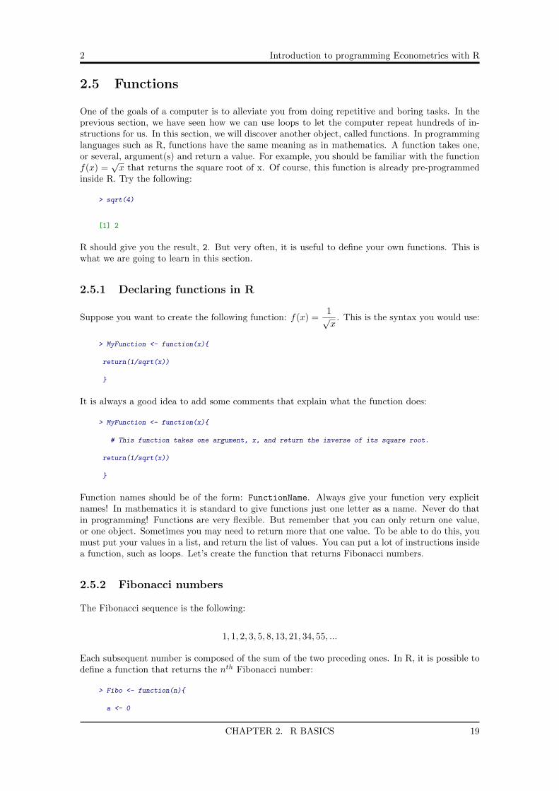
One of the goals of a computer is to alleviate you from doing repetitive and boring tasks. In theprevious section, we have seen how we can use loops to let the computer repeat hundreds of in-structions for us. In this section, we will discover another object, called functions. In programminglanguages such as R, functions have the same meaning as in mathematics. A function takes one,or several, argument(s) and return a value. For example, you should be familiar with the functionf(x) =

√x that returns the square root of x. Of course, this function is already pre-programmed

inside R. Try the following:

> sqrt(4)

[1] 2

R should give you the result, 2. But very often, it is useful to define your own functions. This iswhat we are going to learn in this section.

2.5.1 Declaring functions in R

Suppose you want to create the following function: f(x) =1√x

. This is the syntax you would use:

> MyFunction <- function(x){

return(1/sqrt(x))

}

It is always a good idea to add some comments that explain what the function does:

> MyFunction <- function(x){

# This function takes one argument, x, and return the inverse of its square root.

return(1/sqrt(x))

}

Function names should be of the form: FunctionName. Always give your function very explicitnames! In mathematics it is standard to give functions just one letter as a name. Never do thatin programming! Functions are very flexible. But remember that you can only return one value,or one object. Sometimes you may need to return more that one value. To be able to do this, youmust put your values in a list, and return the list of values. You can put a lot of instructions insidea function, such as loops. Let’s create the function that returns Fibonacci numbers.

2.5.2 Fibonacci numbers

The Fibonacci sequence is the following:

1, 1, 2, 3, 5, 8, 13, 21, 34, 55, ...

Each subsequent number is composed of the sum of the two preceding ones. In R, it is possible todefine a function that returns the nth Fibonacci number:

> Fibo <- function(n){

a <- 0



b <- 1

for (i in 1:n){

temp <- b

b <- a

a <- a + temp

}

return(a)

}

Inside the loop, we defined a variable called temp. Defining temporary variables is usually veryuseful inside loops. Let’s try to understand what happens inside this loop:

1. First, we assign the value 0 to variable a and value 1 to variable b.

2. We start a loop, that goes from 1 to n.

3. We assign the value inside of b to a temporary variable, called temp.

4. b becomes a.

5. We assign the sum of a and temp to a.

6. When the loop is finished, we return a.

What happens if we want the 3rd Fibonacci number? At n = 1 we have first a = 0 and b = 1,then temp = 1, b = 0 and a = 0 + 1. Then n = 2. Now b = 0 and temp = 0. The previousresult, a = 0 + 1 is now assigned to b, so b = 1. Then, a = 1 + 0. Finally, n = 3. temp = 1

(because b = 1), the previous result a = 1 is assigned to b and finally, a = 1 + 1. So the thirdFibonacci number equals 2. Reading this might be a bit confusing; I strongly advise you to runthe algorithm on a sheet of paper, step by step.

The above algorithm is called an iterative algorithm, because it uses a loop to compute the result.Let’s look at another way to think about the problem, with a recursive algorithm.

> FiboRecur <- function(n){

if (n == 0 || n == 1){

return(n)} else {

return(FiboRecur(n-1) + FiboRecur(n-2))

}

}

This algorithm should be easier to understand: if n = 0 or n = 1 the function should return n

(0 or 1). If n is strictly bigger than 1, FiboRecur should return the sum of FiboRecur(n-1)

and FiboRecur(n-2). This version of the function is very much the same as the mathematicaldefinition of the Fibonacci sequence. So why not use only recursive algorithms then? Try to runthe following:

> system.time(Fibo(30))

user system elapsed

0.000 0.001 0.000



The result should be printed very fast (the system.time() function returns the time that it tookto execute Fibo(30)). Let’s try with the recursive version:

> system.time(FiboRecur(30))

user system elapsed

3.177 0.003 3.181

It takes much longer to execute! Recursive algorithms are very CPU demanding, so if speed iscritical, it’s best to avoid recursive algorithms. Also, in FiboRecur try to remove this: if (n ==

0 || n == 1) and try to run FiboRecur(5) for example and see what happens. You should getan error: this is because for recursive algorithms you need a stopping condition, or else, it wouldrun forever. This is not the case for iterative algorithms, because the stopping condition is the laststep of the loop.

Exercises

Write the answers to this exercise inside a file called yourname functions.R and send it to me:[email protected]. Use comments to explain what you do!

Exercise 1 In this exercise, you will write a function to compute the sum of the n first integers.Combine the algorithm we saw in section 2.4.3 and what you learned about functions in this section.

Exercise 2 Write a function called MyFactorial that computes the factorial of a number n. Do ititeratively and recursively.

Exercise 3 In this exercise, we will find the eigenvalues of the following matrix:

A =

(3 11 3

)For this exercise, we will first think about the problem at hand, and try to simplify it as much aspossible before writing any code.

Remember that if A is full column rank, there will be 2 eigenvalues. Also, remember that the sumof the eigenvalues equals the trace of the matrix and that the product of the eigenvalues equalsthe determinant of the matrix. This gives you a system of 2 equations. Replace one equation intothe other. What do you get? What is it that you finally have to do? Program a function to solveyour problem now.

2.6 Preprogrammed functions available in R

In R, a lot of mathematical functions are readily available. We already saw the sqrt() functionin the previous section. In this section, we will take a look to some of the more useful functionsyou need to know about.

2.6.1 Numeric functions

• abs(x): return the absolute value of x

• sqrt(x): return the square root of x

• round(x, digits = n): round a number to the nth place



• exp(x): return the exponential of x

• log(x): return the natural log of x

• log10(x): return the common log of x

• cos(x), sin(x), tan(x): trigonometric functions

• factorial(x): return the factorial of x

• sum(x): if x is a vector, return the sum of its elements

• min(x): if x is a vector, return the smallest of its elements

• max(x): if x is a vector, return the biggest of its elements

2.6.2 Statistical and probability functions

• dnorm(x): return the normal density function

• pnorm(q): return the cumulative normal probability for quantile q

• qnorm(p): return the quantile at percentile p

• rnorm(n, mean = 0, sd = 1): return n random numbers from the standard normal distri-bution

• mean(x): if x is a vector of observations, return the mean of its elements

• sd(x): if x is a vector of observations, return its standard deviation

• cor(x): gives the linear correlation coefficient

• median(x): if x is a vector of observations, return its median

• table(x): makes a table of all values of x with frequencies

• summary(x): if x is a vector, return a number of summary statistics for x

It is also possible to replace the word norm by unif to get the same functions but for the uniformdistribution, pois for poisson, binom for the binomial etc.

2.6.3 Matrix manipulation

In the following definitions, A and B are both matrices of conformable dimensions.

• A * B: return the element-wise multiplication of A and B

• A %*% B: return the matrix multiplication of A and B

• A %x% B or kronecker(A, B): return the Kronecker product of A and B

• t(A): return the transpose of A

• diag(A): return the diagonal of A

• eigen(A): return the eigenvalues and eigenvectors of A

• chol(A): Choleski factorization of A

• qr(A): QR decomposition of A



2.6.4 Other useful commands

• rep(a, n): repeat a n times

• seq(a,b,k): creates a sequence of numbers from a to b, by step k

• cbind(n1, n2, n3,...): creates a vector of numbers

• c(n1, n2, n3, ...): similar to cbind, but the resulting object doesn’t have a dimension

• typeof(a): check the type of a

• dim(a): chick dimension of a

• length(a): returns length of a vector

• ls(): lists memory contents (doesn’t take an argument)

• sort(x): sort the values of vector x

• ?keyword: looks up help for keyword. keyword must be an existing command

• ??keyword: looks up help for keyword, even if the user is not sure the command exists

2.7 Putting it all together

2.7.1 Maximum Likelihood estimation

The goal of this section is to teach you about Maximum Likelihood estimation. After a shorttheoretical reminder, we will see how we can program our own likelihood function and use R tomaximize it.

Theoretical reminder and motivation

Maximum likelihood estimation (and its variants) is probably the most used method to estimateparameters of a statistical model. The idea is the following: given a fixed data set, one writes downthe likelihood function of the underlying data generating process, usually called the model, whichgives the probability of the whole data set, as a function of the parameters. Then, to make thedata set as likely as possible, one finds the parameters that maximize the likelihood function. Invery simple cases, there is no need to perform maximum likelihood estimation as there are closedform solutions for the parameters. For example, for a linear model:

Y = X ′β + ε

one can get β with the following formula:

β = (X ′X)−1X ′Y.

However, in more general and complicated cases, such a nice closed form solution does not existand you will need to program your own likelihood function. Of course, there are functions in R thatestimate the most standard models. For example, to estimate the parameters of a linear model inR you can use the lm() function:

> lm(y ~ x)

where y is a vector and x is a matrix. The command lm regresses y on x and returns β. However,the goal of this section is to review everything we have learned until now by writing our ownlikelihood function and then maximize it.



A simple example: tossing an unfair coin

Suppose we have an unfair coin, but do not know with which probability it falls on head (ortails). The first thing we can do is observe a sequence of throws. For the sake of the exercise,let us suppose that this probability is 0.7. We will first generate data, and then, using maximumlikelihood, try to find this value of 0.7 again.

To generate data from a binomial distribution, run the following command:

> proba <- 0.7

> mydata <- rbinom(100, 1, proba)

This will create a vector of data with 100 observations from a binomial distribution, with P (Xi =1) = 0.7. Now suppose you give this data to your colleague and ask him to find the value of proba(or the parameter of the model) that generated this data. Your colleague knows that the datagenerating process behind this data set must be a binomial distribution, because your observationsonly take on two values, 0 or 1. He knows that the log-likelihood for the binomial model is this6:

log(L) =

n∑i=1

yi ∗ log(p) + (1− yi) ∗ log(1− p)

He then writes this log-likelihood in R:

> BinomLogLik <- function(data, proba){

result <- 0

for(i in 1:length(data)){

result <- result + (data[i] * log(proba) + (1 - data[i]) * log(1 - proba))

}

return(result)

}

Below is another way to write the log-likelihood7:

> BinomLogLik2 <- function(data, proba){

result <- 0

for (i in 1:length(data)){

if (data[i] == 1){

result <- result + log(proba)

}

else {

result <- result + log(1-proba)

}

}

return(result)

}

6And most importantly, he forgot that there is a very simple solution to find the parameter very fast...7From: http://www.johnmyleswhite.com/notebook/2010/04/21/doing-maximum-likelihood-estimation-by-hand-in-r/


http://www.johnmyleswhite.com/notebook/2010/04/21/doing-maximum-likelihood-estimation-by-hand-in-r/


Usually, a likelihood function always has at least two arguments: the data, and a vector of pa-rameters. Here we don’t have a vector but only a scalar, because there is only one parameter toestimate.

There is still one step missing: this likelihood function must be maximized to recover the estimatedvalue of p. For this, we use the optim function in R:

> optim(par = 0.5, fn = BinomLogLik, data = mydata, method="Brent",

lower=0, upper=1, control = list(fnscale= -1))

This function takes a lot of arguments:

• par is an initial value for the parameter. Your colleague chose 0.5, because that’s the prob-ability that a fair coin lands on heads or tails, but he could have chosen any other value.Usually, it is a good idea to try to find good initial values

• fn is the function to maximize, here BinomLogLik

• data is the argument of our function BinomLogLik. You need to specify every other argumentlike this

• method this is the optimization method to use. For problems one-dimensional problems,you must use Brent. If you don’t specify a method, optim will use the Nelder and Meadalgorithm but it only works for multi-dimensional problems. So here, you have to use theBrent method

• lower and upper are the lower and upper bounds to look for the parameter. It is always agood idea to specify bounds, if possible

• control = list(fnscale = -1) By default, optim performs minimization, but with thisoption it will perform maximization. You can add more arguments to this list, if necessary.

Another way to maximize the log-likelihood, is to minimize the negative of the log-likelihood:

> MinusBinomLogLik <- function(data, proba){

result <- 0

for(i in 1:length(data)){

result <- result + (data[i] * log(proba) + (1 - data[i]) * log(1 - proba))

}

return(-result)

}

The only difference with the above function is the minus sign in the return statement. We cannow minimize this function, which is equivalent to maximization of the first function:

> optim(par = 0.5, fn = MinusBinomLogLik, data = mydata, method="Brent",

lower=0, upper=1)

$par

[1] 0.67

$value

[1] 63.41786

$counts

function gradient

NA NA



$convergence

[1] 0

$message

NULL

$par is the value of the estimated parameter and is equal to 0.77 which is quite close to the truevalue, 0.7. $value is the value of the likelihood at this point. The other useful thing to look atis $convergence. This tells you if the optimization algorithm converged correctly. This is veryimportant to know, because if the algorithm didn’t converge, it means that you may need to useanother algorithm or change some options.

Exercise 1 The goal of this exercise is to make you write and maximize your own likelihood function.For this, you will need to download and import some data into R. First download the data here:https://www.dropbox.com/s/tv1difslka6jvy0/data_mle.csv?dl=0 and save it somewhere onyour computer. Then, from Rstudio, go to the Environment tab, and then click on Import Dataset.Select the dataset from earlier and leave all the options as they are.

Just one more step before you continue; write this in your script:

> data_mle <- data_mle$x

This way, your data is only a vector instead of a data frame. Don’t think too much about it fornow, we will learn about all this in the next chapter. Once you have imported the data, you cannow start thinking about which probability density, or mass, function to choose. Take a look atthe data (type data mle in the console). What do you notice? It’s also a good idea to take alook at some descriptive statistics and a graph. Try mean(data mle). This should give you a hintabout the value of the parameter you’re looking for. Also, try this: hist(data mle) (in the nextchapter we will learn more about hist). One more hint: the data was generated with a density(or mass) function with only one parameter. Now, write the likelihood function in R!

Now that you have written down the likelihood in R, it’s a good idea to plot it. We didn’t talkmuch about plots yet, but don’t worry, this is going to be easy. Create the following vector:

> param <- seq(0.1,10, length.out = length(data_mle))

and now type this:

> plot(param, myLogLik(data_mle, param), type = "l", col = "blue", lwd = 2)

where, of course, you have replaced myLogLik by your own likelihood. Forget about the optionsto plot. What do you see? Do you think this graph can be useful? Can you think of at least tworeasons?

Now, use the optim() function to get the estimated parameter value. Compare it to mean(data mle).Is this surprising?


https://www.dropbox.com/s/tv1difslka6jvy0/data_mle.csv?dl=0

Chapter 3

Applied econometrics with R

Now that you are familiar with R, we can start working with data. There are numerous ways toanalyze data. We will start with descriptive statistics, then plots such as histograms and line plots,and conclude with linear models.

3.1 Importing data

The first step to analyze a data set is to import the data into R. Usually, your data is saved some-where in your computer. R has ”to know” where this data set is to work with it. For this chapter,we are going to work with wage data. The data is taken from An Introduction to classical econo-metric theory (Oxford University Press, 2010). You can download the data set and a descriptionhere: https://www.dropbox.com/s/32ujx00stvnbcvp/wage.zip?dl=0. My advice: if you areusing a tool such as Dropbox, create a folder in it called something like programming econometricsand inside this folder another one called Wage. Save the data in it. This data set has the .csv

extension which is a very common format to save data. CSV stands for Comma-separated value.As the name implies, columns in such a file are separated with the symbol ,. But the separatorcould be any other symbol! Always open your file to check the separator if you are having troubleto import the file in R.

Now suppose you want to import the data. On my computer, the data is saved in:

/Dropbox/Documents/Work/TDs/Applied Econometrics with R/Data/Wage/wage.csv

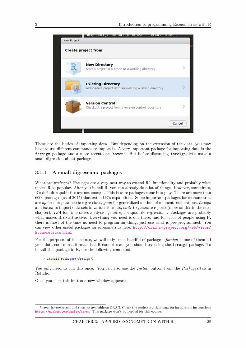
First, we are going to create a new project from Rstudio. In Rstudio, click on File and then NewProject. You should see a window appear with different options. Select the second option ExistingDirectory.

Then select the folder where you save the data. Creating a new project has a lot of advantages. Itis easier to load the data, and everyting you do, such as save figures are exported in that folder.Creating a project also allows you to use Git, a version control system. We are not going to talkabout Git here, however.

Now we can import the data with the command read.csv():

> Wage <- read.csv(file = "Wage.csv", header = T, sep = ",")

The header = T part means that the first line of the file contains a header, or simply the names ofthe columns. The columns are separated by a , symbol, so you need to add this with the optionsep = ",". In some cases, columns may be separated with different separators so this is whereyou can specify them.

27

https://www.dropbox.com/s/32ujx00stvnbcvp/wage.zip?dl=0


These are the basics of importing data. But depending on the extension of the data, you mayhave to use different commands to import it. A very important package for importing data is theforeign package and a more recent one, haven1. But before discussing foreign, let’s make asmall digression about packages.

3.1.1 A small digression: packages

What are packages? Packages are a very neat way to extend R’s functionality and probably whatmakes R so popular. After you install R, you can already do a lot of things. However, sometimes,R’s default capabilities are not enough. This is were packages come into play. There are more than6000 packages (as of 2015) that extend R’s capabilities. Some important packages for econometricsare np for non-parametric regressions, gmm for generalized method of moments estimations, foreignand haven to import data sets in various formats, knitr to generate reports (more on this in the nextchapter), TSA for time series analysis, quantreg for quantile regression... Packages are probablywhat makes R so attractive. Everything you need is out there, and for a lot of people using R,there is most of the time no need to program anything, just use what is pre-programmed. Youcan view other useful packages for econometrics here: http://cran.r-project.org/web/views/Econometrics.html

For the purposes of this course, we will only use a handful of packages. foreign is one of them. Ifyour data comes in a format that R cannot read, you should try using the foreign package. Toinstall this package in R, use the following command:

> install.packages("foreign")

You only need to run this once. You can also use the Install button from the Packages tab inRstudio:

Once you click this button a new window appears:

1haven is very recent and thus not available on CRAN. Check the project’s github page for installation instructionshttps://github.com/hadley/haven. This package won’t be needed for this course.

CHAPTER 3. APPLIED ECONOMETRICS WITH R 28

http://cran.r-project.org/web/views/Econometrics.html

http://cran.r-project.org/web/views/Econometrics.html

https://github.com/hadley/haven


From this window you can then download packages. Once a package is installed, you need to loadit to be able to use it. For this, always write at the top of your script the following line:

> library("foreign")

To know more about a package, it is always useful to read the associated documentation:

> help(package=foreign)

You can also achieve this by clicking on the package’s name in the Packages tab in Rstudio.

It is also possible to write your own packages with your own functions. This is a very clean wayto share your source code among colleagues. We won’t see how to create our own packages in thiscourse, but if you’re interested, I highly recommend R packages by Hadley Wickham.2

2http://r-pkgs.had.co.nz/


http://r-pkgs.had.co.nz/


3.1.2 Back to importing data

To make your life easier, it is possible to import data using Rstudio. For this, click on theEnvironment tab and then the Import Dataset button:

You can then navigate to the folder where you saved your data and click on it. The followingwindow will appear:

The bottom right window is a preview of your data. Here it looks good, so we can click on import.Now look at the Console tab. You should see the command read.csv() appear with the wholepath to the data set. Loading data through Rstudio’s GUI only works for .csv files though.

You also will encounter data in the .xlsx format, which is the format used by Microsoft Excel.There are packages to read such data, but the best is to save your Excel sheet into a .csv file.You can do this directly from Excel or Libreoffice. Once you saved the data in the .csv format, itis easy to import it in Rstudio. Now that you imported the data, we can start working with it.



3.2 One last data type: the data frame type

Data that is loaded in an R session is usually of a special type, called data frame. It is nothingmore that a list of vectors, with some useful attributes such as column names. Knowing how towork on data frames is important, because more often than not, data is very messy and you needto clean it before using it. Manipulation of data frames is outside the scope of this introductorybook. If you want to know more about data frame manipulation, you can learn more about thedplyr package3 that makes these kind of tasks very easy. You should take a look at dplyr if youplan on being serious with data analysis.

3.3 Summary statistics

One of the first steps analysts do after loading data is look at descriptive statistics and plots. Avery useful command for this is summary():

> summary(Wage)

w fe nw un

Min. : 0.84 Min. :0.0000 Min. :0.0000 Min. :0.000

1st Qu.: 6.92 1st Qu.:0.0000 1st Qu.:0.0000 1st Qu.:0.000

Median :10.08 Median :0.0000 Median :0.0000 Median :0.000

Mean :12.37 Mean :0.4973 Mean :0.1528 Mean :0.159

3rd Qu.:15.63 3rd Qu.:1.0000 3rd Qu.:0.0000 3rd Qu.:0.000

Max. :64.08 Max. :1.0000 Max. :1.0000 Max. :1.000

ed ex age wk

Min. : 0.00 Min. : 0.00 Min. :18.00 Min. :0.0000

1st Qu.:12.00 1st Qu.: 9.00 1st Qu.:29.00 1st Qu.:0.0000

Median :12.00 Median :18.00 Median :37.00 Median :0.0000

Mean :13.15 Mean :18.79 Mean :37.93 Mean :0.4073

3rd Qu.:16.00 3rd Qu.:27.00 3rd Qu.:47.00 3rd Qu.:1.0000

Max. :20.00 Max. :56.00 Max. :65.00 Max. :1.0000

You see the mean, median, 1st and 3rd quartiles, minimum and maximum for every variable inyour data set. Sometimes you only need summary statistics of one variable. You can do that with:

> mean(Wage$w)

[1] 12.36585

To access variable w from data set wage you use the $ symbol. If you need to access this variableoften, you can save it with a shorter name:

> wage <- Wage$w

and to get the mean:

> mean(wage)

[1] 12.36585

Sometimes, it useful to get summary statistics only for a subset of data. Before continuing, hereis the description of the data set:

An extract from the March, 1995 Current Population Survey of the U. S. CensusBureau. 1289 observations, 8 variables, including:

3http://cran.rstudio.com/web/packages/dplyr/vignettes/introduction.html


http://cran.rstudio.com/web/packages/dplyr/vignettes/introduction.html


• w: wage

• fe: female indicator variable

• nw: nonwhite indicator variable

• un: union indicator

• ed: years of schooling

• ex: years of potential experience

• wk: weekly earnings indicator variable

For easier access, it is a good idea to save the columns you need inside new variables:

> fe <- Wage$fe

> nw <- Wage$nw

> un <- Wage$un

> ed <- Wage$ed

> ex <- Wage$ex

> wk <- Wage$wk

There is a way to do that faster in R, with the command attach:

> attach(Wage)

This gives you access directly to the columns of wage. Be careful though: sometimes, you mayload more than one dataset which can potentially have columns with the same names. It is goodpractice to save the columns you need in new variables with explicit names, for example:

> fe_d1 <- data_set1$fe

> fe_d2 <- data_set2$fe

3.3.1 Conditional summary statistics

Let’s say you are only interested in knowing the mean of wage for women. You can achieve witharray slicing :

> mean(wage[fe == 1])

[1] 10.59367

This means ”return the mean of wage$w where wage$fe equals 1”. This also works with summary()

of course. You can add any condition you need.

Another useful function to know is table. This gives the frequencies of a variable:

> table(fe)

fe

0 1

648 641

To get the relative frequencies, you can divide by the number of observations:

> table(fe) / length(fe)

fe

0 1

0.5027153 0.4972847



3.3.2 Getting descriptive statistics easier with dplyr

dplyr is one of the packages developed by Hadley Wickham, assistant professor at Rice Universityand R guru. With dplyr getting summary statistics is easier than with the built-in R commands.For this, you must learn a new operator, %>% which is called ”pipe”. In computing, piping is anold and very useful concept. The best way to understand this new operator is with an example.Let’s define a function:

> my_f <- function(x){

return(x+x)

}

This function takes a number x and returns x+x. Very simple. One way to use it in R is like this:

> my_f(3)

[1] 6

which returns 6. Now, let’s use %>% (do not forget to load the dplyr package first!):

> library(dplyr)

> 3 %>% my_f()

[1] 6

and this also returns 6. What %>% does is that it passes the object on the left hand side as thefirst argument of the function on the right hand side. This may seem more complicated than theusual way of doing things, but you’ll will see very shortly that it actually increases readability.

Let’s try the following: what is the average wage for people of different races? This can be donevery easily with the dplyr package:

> Wage %>% group_by(nw) %>% summarise(mean(w))

Source: local data frame [2 x 2]

nw mean(w)

1 0 12.794423

2 1 9.990203

The command is read like this: ”take the wage data set and pipe it to the function group by4 andnow pipe this data set grouped by race to the function summarise. Finally, the function summarise

will compute the mean of the wage, by race”. Without the %>% operator, this would look like this:

> summarise(group_by(Wage, nw), mean(w))

which is much less readable than above. If you want to have the average wages by education leveland marital status, you do it this way:

> Wage %>% group_by(nw, fe) %>% summarise(mean(w))


Groups: nw

4A function from the dplyr package.



nw fe mean(w)

1 0 0 14.573417

2 0 1 10.928649

3 1 0 11.264045

4 1 1 8.940463

If you want more descriptive statistics, just add more summary functions:

> Wage%>% group_by(nw, fe) %>% summarise(min(w), mean(w), max(w))


Groups: nw

nw fe min(w) mean(w) max(w)

1 0 0 1.15 14.573417 49.46

2 0 1 0.84 10.928649 64.08

3 1 0 1.57 11.264045 36.05

4 1 1 2.08 8.940463 25.48

You can also save these summary statistics inside variables:

> wage_by_nw <- Wage %>% group_by(nw, fe) %>% summarise(min(w), mean(w), max(w))

But to make it look even better you can use another operator: ->

> Wage %>% group_by(nw) %>% summarise(min(w), mean(w), max(w)) -> wage_by_nw

This reads like this: ”take the wage data set, group it by race and gender, return the minimum,mean and maximum for these groups and save this table inside wage by nw”. dplyr is capable ofmuch more, but we won’t look into the rest of dplyr’s functionality. For more info, you can take alook at the Data Wrangling with dplyr and tidyr Cheat Sheet here: http://www.rstudio.

com/wp-content/uploads/2015/01/data-wrangling-cheatsheet.pdf.

3.4 Plots

After summary statistics, it also a very good idea to make some plots of the data. There are twomain commands that you need to know, hist and plot. hist creates histograms. Histograms areused for discrete data. Age is expressed in years, so it is discrete. In our data set age only has ahandful of values. We can know how many like this:

> length(unique(ed))

[1] 12

We see that ed only has 12 unique values. To have a visual representation of ed a histogram isthus suited.

3.4.1 Histograms

To get a basic histogram, use the hist() command:

> hist(ed)


http://www.rstudio.com/wp-content/uploads/2015/01/data-wrangling-cheatsheet.pdf

http://www.rstudio.com/wp-content/uploads/2015/01/data-wrangling-cheatsheet.pdf


Histogram of ed

ed

Fre

quen

cy

0 5 10 15 20

020

040

060

0

You can add color, change the name of the plot and much more with different options:

> hist(ed, main = "Histogram of education", xlab = "Education", ylab = "Density",

freq = F, col = "light blue")



Histogram of education

Education

Den

sity

0 5 10 15 20

0.00

0.05

0.10

0.15

0.20

0.25

0.30

You can switch from densities to frequencies by changes the option freq = F to freq = T. Youcan also add more options, such as the limits of the x and y axis and add a grid:

> hist(ed, main = "Histogram of education", xlab = "Education",

ylab = "Frequency", freq = F, col = "light blue",

ylim = c(0, 0.4), xlim = c(0,20))

> grid()



Histogram of education

Education

Fre

quen

cy

0 5 10 15 20

0.0

0.1

0.2

0.3

0.4

Consult hist’s help to learn about all the options I used above.

3.4.2 Scatter plots and line graphs

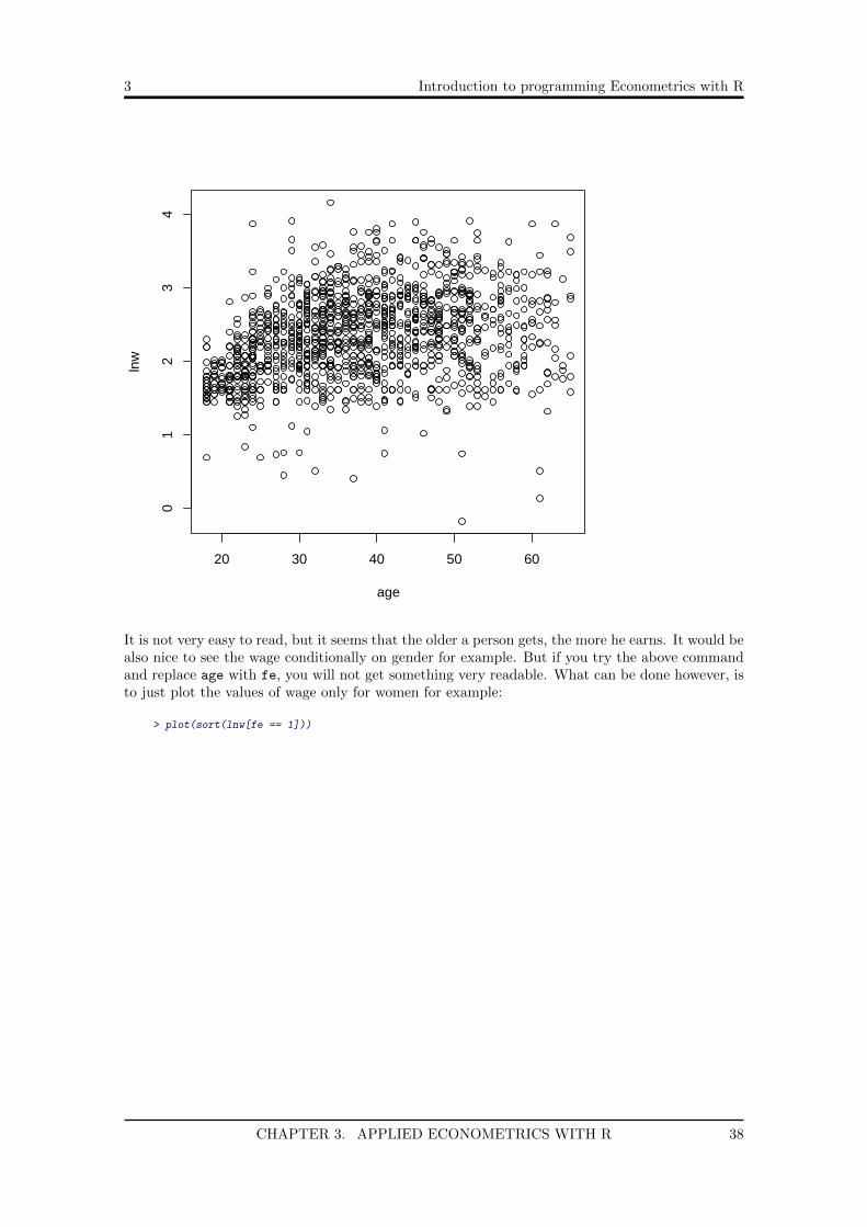
When graphing wages, it is usually useful to graph the log of the wage instead of just the wage.Let’s define a new variable:

> lnw <- log(w)

Scatter plots can display values for two variables. Try the following:

> plot(age, lnw)



20 30 40 50 60

01

23

4

age

lnw

It is not very easy to read, but it seems that the older a person gets, the more he earns. It would bealso nice to see the wage conditionally on gender for example. But if you try the above commandand replace age with fe, you will not get something very readable. What can be done however, isto just plot the values of wage only for women for example:

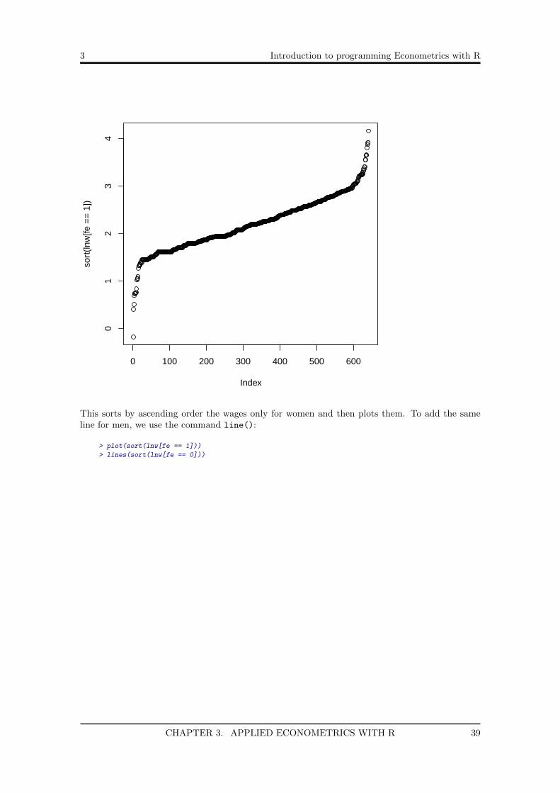
> plot(sort(lnw[fe == 1]))



0 100 200 300 400 500 600

01

23

4

Index

sort

(lnw

[fe =

= 1

])

This sorts by ascending order the wages only for women and then plots them. To add the sameline for men, we use the command line():

> plot(sort(lnw[fe == 1]))

> lines(sort(lnw[fe == 0]))



0 100 200 300 400 500 600

01

23

4

Index

sort

(lnw

[fe =

= 1

])

This is not very readable. Let’s make it better by adding colors and a legend:

> plot(sort(lnw[fe == 1]), col = "red", ylab = "Log(Wage)",

main = "Wage by gender", type = "l", lwd = 4)

> lines(sort(lnw[fe == 0]), col = "blue", lwd = 4)

> legend("topleft", legend = c("Women", "Men"), pch = "_", col = c("red", "blue"))



0 100 200 300 400 500 600

01

23

4Wage by gender

Index

Log(

Wag

e)

__

WomenMen

This is the result we get in the end:

This already looks much better. To add the legend to the plot, we used the legend() command,with different options, to specify where we want the legend, and what we want in it. The pch

option allows you to change the symbols that appear in the legend. Since we are only using lines(as specified by the option type = "l") I put the symbol " ". The option lwd() allows you tochange the line width. Change these values and see what happens!



3.5 Linear Models

Linear regression models are the most simple type of statistical models that you can use to analyzea dependent variable, conditionally on explanatory variables. A linear model in matrix notationlooks like this:

Y = X ′β + epsilon

Here, an economists tries to show how a dependent variable Y varies with X. X is a matrix whereeach column is an explanatory variable. For example, one might be interested in the different wagelevels for people with different socio-economic backgrounds and/or education levels, age, etc.

But why not just compute means and compare? For example, let’s say we want to compare thewages of white and nonwhite workers in the US. Using the data from the previous section, we couldcompute the means for these groups like this:

> mean(lnw[nw == 1])

[1] 2.157817

> mean(lnw[nw == 0])

[1] 2.375718

We get a result of 2.38 for white workers and 2.16 (both in logs) for black workers, and concludethat black workers earn less because of racism in the US and go to the bar next to the facultyand enjoy a hard-earned Alsatian beer. However, this analysis may be too simple to reach thatconclusion. Remember, correlation does not equal causation. What if we also control for gender?For example, the following commands compute the wage for female white and black workers:

> mean(lnw[nw == 1 & fe == 1])

[1] 2.074618

> mean(lnw[nw == 0 & fe == 1])

[1] 2.221696

As you can see, the gap is smaller for female workers than for male workers. What if we controlfor education? More specifically, let’s focus on women with less that 12 years of schooling:

> mean(lnw[nw == 1 & ed < 12 & fe == 1])

[1] 1.7153

> mean(lnw[nw == 0 & ed < 12 & fe == 1])

[1] 1.726739

The gap keeps getting lower. We cannot keep adding variables like this however, because we havea lot of them, and these variable can take on a lot of different values. A simple way to study theproblem at hand is to estimate a linear model. If we go back to the equation of a linear modeldefined at the start of the section, what we want to have is β which is the vector of parameters ofthe model. Let us suppose we want to estimate the parameters of the following model:



wage = β0 + β1 ∗ nw + β2 ∗ ed+ β3 ∗ fe+ ε.

β0 is called the intercept. Different approaches are possible to estimate β0, β1, β2 and β3. For thelinear model, we have a closed form solution for the vector of parameters β:

β = (X ′X)−1X ′Y

where X is the following matrix

X =

1 nw1 ed1 fe11 nw2 ed2 fe2...

......

...1 nwN edN feN

The first column, which only contains ones is for the intercept. The other columns contain theobserved values for variable nw and ed. How would you create the vector of estimated parameterswith R? First, you need to create the matrix X. Recall the commands we’ve seen in the previouschapters:

> X <- cbind(1, nw, ed, fe)

We should have a matrix that has 4 columns and 1289 lines (because we have 3000 observationsin our data set):

> dim(X)

[1] 1289 4

returns 1289 lines and 4 columns indeed. What more do we need? It would be useful to have thetranspose of X:

> tX <- t(X)

and we have all we need to compute β:

> beta_hat <- solve(tX %*% X) %*% tX %*% lnw

You should get the following result for beta hat:

> print(beta_hat)

[,1]

1.31131883

nw -0.14029955

ed 0.09025108

fe -0.26909763

What does it mean? Suppose that you want to predict the wage of a female, nonwhite worker andcontrol by schooling years. You would simply compute it like this:

lnw = 1.311− 0.14 ∗ 1 + 0.09 ∗ 1− 0.27 ∗ 1

You simply use the obtained results and replace the values of nw, ed and fe for which you want toget the predicated wage. The intercept can be interpreted as the minimum wage. For each year



of supplementary schooling the individual gets 0.09 log dollars added to her wage. But being awoman carries a penalty of -0.27 log dollars.

The second method you can use to obtain the same result is to use the command lm(). Run thefollowing and see what happens:

> lm(lnw ~ nw + ed + fe)

Call:

lm(formula = lnw ~ nw + ed + fe)

Coefficients:

(Intercept) nw ed fe

1.31132 -0.14030 0.09025 -0.26910

You should obtain the very same result. The difference between the two methods is that the lm()

function does not use the closed form solution from before, but uses a numerical procedure, justlike we did at the end of the previous chapter with the optim() function. If you want more detailsyou can use summary() with lm():

> model <-lm(lnw ~ nw + ed + fe)

> summary(model)

Call:

lm(formula = lnw ~ nw + ed + fe)

Residuals:

Min 1Q Median 3Q Max

-2.25457 -0.32683 0.01351 0.33678 1.96729

Coefficients:

Estimate Std. Error t value Pr(>|t|)

(Intercept) 1.311319 0.069899 18.760 < 2e-16 ***

nw -0.140300 0.039215 -3.578 0.000359 ***

ed 0.090251 0.005014 17.998 < 2e-16 ***

fe -0.269098 0.028128 -9.567 < 2e-16 ***

---

Signif. codes: 0 ‘***’ 0.001 ‘**’ 0.01 ‘*’ 0.05 ‘.’ 0.1 ‘ ’ 1

Residual standard error: 0.5043 on 1285 degrees of freedom

Multiple R-squared: 0.2621, Adjusted R-squared: 0.2604

F-statistic: 152.2 on 3 and 1285 DF, p-value: < 2.2e-16

The second column of summary() is very important, because it shows the standard errors of theestimated parameters. We see that the standard errors are very small, and that the t values arelarger than 2. What this means is that the coefficient is different from 0 at the 5% threshold. Lookat the last column: this shows you the critical probabilities. They’re all much smaller than 0.05,meaning, again, that the coefficients are different from 0 at the 5% threshold.

Exercises

Exercise 1

Estimate the parameters of the following model:

wage = β0 + β1 ∗ nw + β2 ∗ ed+ β3 ∗ un+ β4 ∗ fe+ β5 ∗ age+ ε.

with the closed form solution formula. Also use the closed form solution to obtain the estimationof the standard error of the parameters:



SE(β) =√σ2 ∗ (X ′X)−1jj

(jj means that we only need the diagonal elements of the matrix (X ′X)−1 ) where σ2 is replacedby its estimation s2:

s2 =e′e

n− p=

(Y −Xβ)′(Y −Xβ)

n− p

where n is the number of observations and p is the number of estimated parameters. Compareyour results with the results obtained with lm().

How can you get the t values? Take a close look at your estimated parameters and the standarderrors. Then take a close look a the t values. Notice something?

Now estimate this model:

wage = β0 + β1 ∗ nw + β2 ∗ ed+ β3 ∗ un+ β4 ∗ fe+ β5 ∗ age+ β6 ∗ ex+ ε.

again with both the closed form solution and the lm() function. What happens? Can you think ofa reason of why this happens? Remember that ex is the potential, and not observed, experience.Regress age on a constant, education and experience and see what happens.

Exercise 2

The goal of this exercise is to study the residuals of the regression:

wage = β0 + β1 ∗ nw + β2 ∗ ed+ β3 ∗ un+ β4 ∗ fe+ β5 ∗ age+ ε.

• Using the closed form solution for β, get the estimates of the above model.

• Compute the fitted values: y = X ′β

• Compute the residuals: ε = y − y

• Plot ε.

• Now estimate the same model, but with lm() and save the regression in a variable calledmy model.

• Save the residuals of the regression like this: my residuals <- my model$residuals.

• Plot my residuals and compare it to the previous plot to check if your calculations are right.

Does this residual plot seem good? Why / why not? Take a look at a histogram of the residuals.Thoughts?

What should you expect if you plot the fitted values against the residuals? Take a look at the plot:

> plot(yhat, eps)

Is what you see good? What about:

> plot(lnw, eps)

Is this surprising?

Exercise 3 5

For this exercise, we are going to use data that is available directly from an R package called Ecdat.First install Ecdat:

5Inspired by A guide to modern Econometrics by Marno Verbeek.



> install.packages("Ecdata")

and then you can load the relevant data set:

> library("Ecdat")

> data(Capm)

We are going to study the risk premium of the food, durables and construction industries usingthe Capital asset pricing model. Remember the formula of the CAPM:

E(Ri)−Rf = βi(E(Rm)−Rf )

where E(Ri) is the expected return of the capital asset, Rf is the risk free interest rate, E(Rm) isthe expected return of market and the βi, called the beta is the sensitivity of the expected excessasset returns to the expected excess market return. i indexes the different industries. In our dataset, we already have the risk premium, E(Ri)−Rf as rfood for the food, rcon for the constructionand rdur for the durables industry. The market premium, E(Rm)−Rf is the variable rmrf. Howcan you obtain the βi for the food, durables and construction industries? Pay attention to the factthat there is no intercept in the formula of the CAPM. Compare this result to the formula youshould already now from your introduction to finance course:

βi =Cov(Ri, Rm)

V ar(Rm)

What happens if you estimate the CAPM again, but this time by adding an intercept? Are thereany significant differences between the estimated betas of the model without intercept? Why /why not? Is this surprising?

Now, we want to test for the January effect. First, create a new variable called month that repeatsthe numbers 1 through 12, 43 times (the number of years in the data set). Look into the rep andseq functions. Append this new variable to the data set:

> Capm$month <- month

Now using ifelse(), create a dummy variable for the month of January. Call this dummy jan

and also append it to the data.

Now regress the risk premiums of each industry on a constant, the January dummy and the marketpremium. For each of these industries, is there a positive January effect?


Chapter 4

Reproducible research

4.1 What is reproducible research?

I could not write a better definition than the one you can find on Wikipedia1, so let’s just quotethat:

The term reproducible research refers to the idea that the ultimate product of aca-demic research is the paper along with the full computational environment used to pro-duce the results in the paper such as the code, data, etc. that can be used to reproducethe results and create new work based on the research.

For a study to be credible, people have to be able to reproduce it, this means they need to haveaccess to the data and the computer code of the statistical analysis from the study. Sometimes, itis impossible to share data due to confidentiality issues2 but the code can and should be alwaysshared. How can you trust results if you cannot take a look at the analysis. How can you be surethat the researchers didn’t make a mistake, or worse, are not outright lying?

4.2 Using R and Rstudio for reproducible research

This semester, you will study a topic that interests you using R and Rstudio. You will write areport and send it to me... But you will write the report with Rstudio directly, and not with Wordor Libreoffice. Why not you may ask? Because it’s easier with Rstudio, and you will soon see why.

To start writing a report with Rstudio, click on File → New File → R Markdown...

The following window should pop up:

1https://en.wikipedia.org/wiki/Reproducibility#Reproducible_research2As an example, some researchers in our lab have access to very fine-grained information on 1% of every French

citizen. This includes gender, diploma, wage, taxes paid, etc... The data is accessed remotely and authentication ofthe researchers is made his fingerprints.

47

https://en.wikipedia.org/wiki/Reproducibility#Reproducible_research


Put whatever title you want (you can change this later), your name and leave the rest as is.

Now you should see this in your editor window:

Before doing anything else, read the document; the information written there is basically all youneed to know about R Markdown. Then, click on Knit HTML:

CHAPTER 4. REPRODUCIBLE RESEARCH 48


and wait a few seconds... See what happens? That’s right, you get a document with text and Rcode, and the output directly embedded. If you go back to the Knit HTML button, you can clickon the little triangle at the end of the bottom and create a Word document instead of the HTMLone (leave the PDF option alone. For this, you need LATEXinstalled on your system. If you don’tknow what LATEXis, don’t worry about it). If you then click on Knit Word, Microsoft Word orLibreoffice should open (depending on what’s installed on your computer) with the same outputas for the HTML file. So to summarise: you create a new R Markdown document (notice thatthe extension of a R Markdown document is .Rmd) and in it, you put your R code and directlywrite the text accompanying the code. Then you either knit an HTML file or a .docx file. Bewarethough, sometimes kniting a .docx file doesn’t work very well. In case your document doesn’t looklike how it’s supposed to look, it’s better to knit an HTML document (which you can open withany web browser).

What file do you think you have to share if you want to make your study reproducible? Youguessed it, the .Rmd file. That way, another researcher can re-knit the documents if he wants to,or change them (for example to adapt your code to his own study).

So what you’ll have to do is send me the .Rmd file of your project. As an example, go to the fol-lowing link: https://www.dropbox.com/s/igw645r4xug46mg/maxLike.rmd?dl=0 and downloadthe .Rmd file and knit it! (As I told you above, kniting a .docx file may not always work, and itseems to be case for this file. It’s better to knit an HTML document.) This document shows youhow to write the likelihood of a linear regression model. Do not worry if you find the code in thatdocument complicated for now. Just study the structure of the .Rmd file and try to change things.As you can see in the document, there is not only R code, but also another kind of code between$ sings. This is LATEXcode and is very useful to write mathematical formulas. This is outside thescope of this book so forget about it now. If you need to write formulas, just write them in plaintext like this:

```y = a + b1 * x1 + e

```

To learn more about R Markdown, I strongly invite you to take a look at two cheat sheets madeby the developers of Rstudio:

http://rmarkdown.rstudio.com/RMarkdownCheatSheet.pdf

and

http://rmarkdown.rstudio.com/RMarkdownReferenceGuide.pdf

Do not forget that the goal of R Markdown is to make research reproducible. So don’t forget that


https://www.dropbox.com/s/igw645r4xug46mg/maxLike.rmd?dl=0

http://rmarkdown.rstudio.com/RMarkdownCheatSheet.pdf

http://rmarkdown.rstudio.com/RMarkdownReferenceGuide.pdf


you need to make your code portable. This means that if you share a .Rmd file, the person whodownloads it only has to push Knit HTML to get the document and nothing more. That is whyyou should put the data in the same folder as the .Rmd document. So share the whole folder, andin your .Rmd document load your data with the following command:

> read.csv("data.csv")

and not with the entire path because this is only valid for your computer!
