introduction to multivariate analysis

Lecture #1 - 8/24/2005 Slide 1 of 30

Introduction to Multivariate Analysis

Lecture 1

August 24, 2005Multivariate Analysis

Overview

•Today’s Lecture

Introductions

Course Overview

Data Organization

Descriptive Statistics

Graphical Techniques

Distance Measures

SAS Introduction

Wrapping Up

Lecture #1 - 8/24/2005 Slide 2 of 30

Today’s Lecture

• Introductions.

• Syllabus and course overview.

• Chapter 1 (a brief review, really):

◦ Data organization/notation.

◦ Graphical techniques.

◦ Distance measures.

• Introduction to SAS.

Overview

Introductions

Course Overview

Data Organization



Distance Measures

SAS Introduction

Wrapping Up

Lecture #1 - 8/24/2005 Slide 3 of 30

Who are you?

To help all of use get to know each other better, please tell usyour:

• Name.

• Department and specialty.

• Where you are from originally.

• Where you did you undergraduate work.

Overview

Introductions

Course Overview

•Multivariate

Data Organization



Distance Measures

SAS Introduction

Wrapping Up

Lecture #1 - 8/24/2005 Slide 4 of 30

Syllabus

Syllabus discussion...

Overview

Introductions

Course Overview

•Multivariate

Data Organization



Distance Measures

SAS Introduction

Wrapping Up

Lecture #1 - 8/24/2005 Slide 5 of 30

Multivariate Statistics

A taxonomy of multivariate statistical analyses shows thatmost techniques fall into one of the following categories:

1. Data reduction or structural simplification.

2. Sorting and grouping.

3. Investigation of the dependence among variables.

4. Prediction.

5. Hypothesis construction and testing.

Overview

Introductions

Course Overview

Data Organization

•Arrays



Distance Measures

SAS Introduction

Wrapping Up

Lecture #1 - 8/24/2005 Slide 6 of 30

Data Organization

• As a precursor of things to come, here is a preview of theways data are organized in this book/course.

• Multivariate data are a collection of observations (ormeasurements) of:

◦ p variables (k = 1, . . . , p).

◦ n “items” (j = 1, . . . , n).

◦ “items” can also be though of assubjects/examinees/individuals or entities (whenpeople are not under study) .

◦ In some disciplines (such as educationalmeasurement), “items” are considered the variablescollected per individual.

Lecture #1 - 8/24/2005 Slide 7 of 30

Data Organization

• xjk = measurement of the kth variable on the jth entity.

Variable 1 Variable 2 . . . Variable k . . . Variable p

Item 1: x11 x12 . . . x1k . . . x1p

Item 2: x21 x22 . . . x2k . . . x2p

......

......

...Item j: xj1 xj2 . . . xjk . . . xjp

......

......

...Item n: xn1 xn2 . . . xnk . . . xnp

Overview

Introductions

Course Overview

Data Organization

•Arrays



Distance Measures

SAS Introduction

Wrapping Up

Lecture #1 - 8/24/2005 Slide 8 of 30

Arrays

• To represent the entire collection of items and entities, arectangular array can be constructed:

X =

x11 x12 . . . x1k . . . x1p

x21 x22 . . . x2k . . . x2p

......

......

xj1 xj2 . . . xjk . . . xjp

......

......

xn1 xn2 . . . xnk . . . xnp

• In the next class, we will learn about how arrays like thishave an algebra that makes life somewhat easier.

• All arrays will be symbolized by boldfaced font.

Overview

Introductions

Course Overview

Data Organization

•Arrays



Distance Measures

SAS Introduction

Wrapping Up

Lecture #1 - 8/24/2005 Slide 9 of 30

Array Example

• So, putting things all together, envision standing outside ofthe Kansas Union Bookstore, asking people for receipts.

• You are interested in looking at two variables:

◦ Variable 1: the total amount of the purchase.

◦ Variable 2: the number of books purchased.

• You find four people, and here is what you see observe(with notation:

x11 = 42 x21 = 52 x31 = 48 x41 = 58

x12 = 4 x22 = 5 x32 = 4 x42 = 3

Overview

Introductions

Course Overview

Data Organization

•Arrays



Distance Measures

SAS Introduction

Wrapping Up

Lecture #1 - 8/24/2005 Slide 10 of 30

Array Example (Continued)

• The data array would the look like:

X =

x11 x12

x21 x22

x31 x32

x41 x42

=

42 4

52 5

48 4

58 3

• Notice for any variable, xjk:

◦ The first subscript (j) represents the ROW location inthe data array.

◦ The second subscript (k) represents the COLUMNlocation in the data array.

Overview

Introductions

Course Overview

Data Organization


•Sample Mean

•Sample Variance

•Sample Correlation


Distance Measures

SAS Introduction

Wrapping Up

Lecture #1 - 8/24/2005 Slide 11 of 30

Descriptive Statistics Review

• When we have a large amount of data, it is often hard toget a manageable description of the nature of the variablesunder study.

• For this reason (and as a way of introducing a review topicsfrom previous courses), descriptive statistics are used.

• Such descriptive statistics include:

◦ Means.

◦ Variances.

◦ Covariances.

◦ Correlations.

Overview

Introductions

Course Overview

Data Organization


•Sample Mean

•Sample Variance



Distance Measures

SAS Introduction

Wrapping Up

Lecture #1 - 8/24/2005 Slide 12 of 30

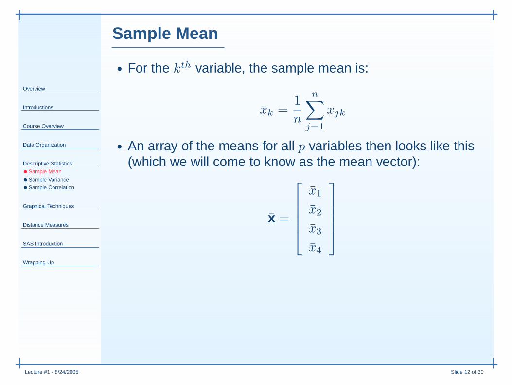
Sample Mean

• For the kth variable, the sample mean is:

x̄k =1

n

n∑

j=1

xjk

• An array of the means for all p variables then looks like this(which we will come to know as the mean vector):

x̄ =

x̄1

x̄2

x̄3

x̄4

Overview

Introductions

Course Overview

Data Organization


•Sample Mean

•Sample Variance



Distance Measures

SAS Introduction

Wrapping Up

Lecture #1 - 8/24/2005 Slide 13 of 30

Sample Variance

• For the kth variable, the sample variance is:

s2

k = skk =1

n

n∑

j=1

(xjk − x̄k)2

• Note the “kk” subscript, this will be important because theequation that produces the variance for a single variable isa derivation of the equation of the covariance for a pair ofvariables.

• Also note the division by n. Reasons for this will becomeapparent in the near future.

• For a pair of variables, i and k, the sample covariance is:

sik =1

n

n∑

j=1

(xji − x̄i)(xjk − x̄k)

Overview

Introductions

Course Overview

Data Organization


•Sample Mean

•Sample Variance



Distance Measures

SAS Introduction

Wrapping Up

Lecture #1 - 8/24/2005 Slide 14 of 30

Sample Covariance Matrix

• Making an array of all sample covariances give us:

Sn =

s11 s12 . . . s1p

s21 s22 . . . s2p

......

. . ....

sp1 sp2 . . . spp

Overview

Introductions

Course Overview

Data Organization


•Sample Mean

•Sample Variance



Distance Measures

SAS Introduction

Wrapping Up

Lecture #1 - 8/24/2005 Slide 15 of 30

Sample Correlation

• Sample covariances are dependent upon the scale of thevariables under study.

• For this reason, the correlation is often used to describethe association between two variables.

• For a pair of variables, i and k, the sample correlation isfound by dividing the sample covariance by the product ofthe standard deviation of the variables:

rik =sik√

sii

√skk

• The sample correlation:◦ Ranges from -1 to 1.◦ Measures linear association.◦ Is invariant under linear transformations of i and k.◦ Is a biased estimator.

Overview

Introductions

Course Overview

Data Organization


•Sample Mean

•Sample Variance



Distance Measures

SAS Introduction

Wrapping Up

Lecture #1 - 8/24/2005 Slide 16 of 30

Sample Correlation Matrix

• Making an array of all sample covariances give us:

R =

1 r12 . . . r1p

r21 1 . . . r2p

......

. . ....

rp1 rp2 . . . 1

Overview

Introductions

Course Overview

Data Organization



•Bivariate Scatterplots

•Trivariate Scatterplots

•Stars

•Chernoff Faces

•Dendrograms

•Variable Space

•Network Diagrams

Distance Measures

SAS Introduction

Wrapping Up

Lecture #1 - 8/24/2005 Slide 17 of 30


• Displaying multivariate data can be difficult due to ournatural limitations of 3-dimensions.

• Several simple ways of displaying data include:

◦ Bivariate scatterplots.

◦ Three-dimensional scatterplots.

• But you already know those, some plots that can beachieved by multivariate methods include:◦ “Stars.”

◦ Chernoff faces.

Lecture #1 - 8/24/2005 Slide 18 of 30

Bivariate Scatterplots

Lecture #1 - 8/24/2005 Slide 19 of 30

Trivariate Scatterplots

Overview

Introductions

Course Overview

Data Organization



•Bivariate Scatterplots

•Trivariate Scatterplots

•Stars

•Chernoff Faces

•Dendrograms

•Variable Space

•Network Diagrams

Distance Measures

SAS Introduction

Wrapping Up

Lecture #1 - 8/24/2005 Slide 20 of 30


• But you already know those plots.

• Some plots that can be achieved by multivariate methodsinclude:

◦ “Stars.”

◦ Chernoff faces.

◦ Dendrograms.

◦ Bivariate plots, but of the variable space.

◦ Network graphs.

Lecture #1 - 8/24/2005 Slide 21 of 30

Stars

Lecture #1 - 8/24/2005 Slide 22 of 30

Chernoff Faces

Lecture #1 - 8/24/2005 Slide 23 of 30

Dendrograms

Lecture #1 - 8/24/2005 Slide 24 of 30

Variable Space Plots

Lecture #1 - 8/24/2005 Slide 25 of 30

Network Diagrams

P000000

P000001

P000010

P000011

P000100

P000101

P000110

P000111

P001000

P001001

P001010

P001011

P001100

P001101

P001110

P001111

P010000

P010001

P010010

P010011

P010100

P010101

P010110

P010111

P011000

P011001

P011010

P011011

P011100

P011101

P011110

P011111

P100000

P100001

P100010

P100011

P100100

P100101

P100110

P100111

P101000

P101001

P101010

P101011

P101100P101101

P101110

P101111

P110000

P110001

P110010

P110011

P110100

P110101

P110110

P110111

P111000

P111001

P111010

P111011

P111100

P111101

P111110

P111111

Pajek

Overview

Introductions

Course Overview

Data Organization



Distance Measures

SAS Introduction

Wrapping Up

Lecture #1 - 8/24/2005 Slide 26 of 30

Distance Measures

• A great number of multivariate techniques revolve aroundthe computation of distances:

◦ Distances between variables.

◦ Distances between entities.

• The formula for the Euclidean distance formula betweenthe coordinate pair P = (x1, x2) and the origin P = (0, 0):

d(O, P ) =√

x2

1+ x2

2

Overview

Introductions

Course Overview

Data Organization



Distance Measures

SAS Introduction

Wrapping Up

Lecture #1 - 8/24/2005 Slide 27 of 30

Distance Measures

• Elaborate discussions of distance measures will be foundlater in the class

• Just keep in mind that there are statistical analogs todistance measures, taking the variability of variables intoaccount.

• Also be aware that there are literally an infinite number ofdistance measures!

• A distance measure must satisfy the following:

◦ d(P, Q) = d(Q, P )

◦ d(P, Q) > 0 if P 6= Q

◦ d(P, Q) = 0 if P = Q

◦ d(P, Q) ≤ d(P, R) + d(R, Q) (known as the triangleinequality)

Overview

Introductions

Course Overview

Data Organization



Distance Measures

SAS Introduction

Wrapping Up

Lecture #1 - 8/24/2005 Slide 28 of 30

Introduction to SAS

• SAS has a reputation for being...well...unliked by many inthe social sciences.

• Why bother teaching it in this course?

◦ New focus on SAS in our department.

◦ Adding value to your degree (check out amstat.org ordice.com for details).

• For some good things about SAS, check outhttp://www.pbs.org/cringely/pulpit/pulpit20020411.html

Overview

Introductions

Course Overview

Data Organization



Distance Measures

SAS Introduction

Wrapping Up

•Final Thought

•Next Class

Lecture #1 - 8/24/2005 Slide 29 of 30

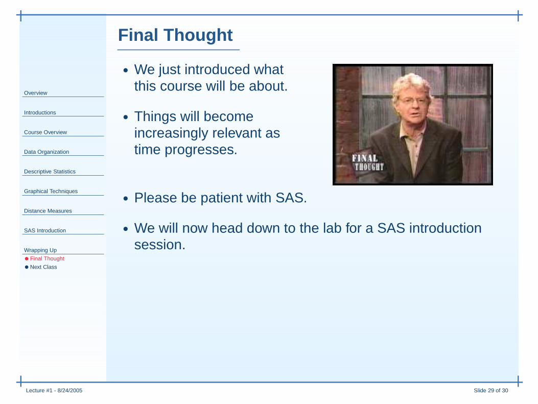
Final Thought

• We just introduced whatthis course will be about.

• Things will becomeincreasingly relevant astime progresses.

• Please be patient with SAS.

• We will now head down to the lab for a SAS introductionsession.

Overview

Introductions

Course Overview

Data Organization



Distance Measures

SAS Introduction

Wrapping Up

•Final Thought

•Next Class

Lecture #1 - 8/24/2005 Slide 30 of 30

Next Time

• Matrix algebra (Chapter 2, Supplement 2A)

• SAS proc iml

introduction to multivariate analysis

Documents