introduction to matlab course...
TRANSCRIPT
Introduction to MatlabCourse notes
Mark Herbster and Jason KastanisCopyright c©2006 M. Herbster and J.Kastanis
January 2006
CONTENTS i
Contents
I Interface Guide 1
1 Overview 1
2 Style of the guide 2
3 A brief history of Matlab 2
4 Basic elements of programming 3
5 Matlab main desktop 45.1 Title bar . . . . . . . . . . . . . . . . . . . . . . . . . . . . . . 55.2 Menu bar . . . . . . . . . . . . . . . . . . . . . . . . . . . . . 55.3 Desktop toolbar . . . . . . . . . . . . . . . . . . . . . . . . . . 65.4 Command window . . . . . . . . . . . . . . . . . . . . . . . . 65.5 Command history . . . . . . . . . . . . . . . . . . . . . . . . . 85.6 Current directory (window) . . . . . . . . . . . . . . . . . . . 85.7 Launch pad . . . . . . . . . . . . . . . . . . . . . . . . . . . . 95.8 Workspace . . . . . . . . . . . . . . . . . . . . . . . . . . . . . 10
6 Opening and editing files 106.1 Opening files . . . . . . . . . . . . . . . . . . . . . . . . . . . 106.2 Editing files . . . . . . . . . . . . . . . . . . . . . . . . . . . . 12
7 Getting help 157.1 Text based help . . . . . . . . . . . . . . . . . . . . . . . . . . 157.2 Graphical interface help . . . . . . . . . . . . . . . . . . . . . 177.3 Web-based help . . . . . . . . . . . . . . . . . . . . . . . . . . 23
8 Setting the desktop layout 24
II Lecture 1 25
9 Overview of Lecture 1 25
10 Style of notes 26
CONTENTS ii
11 Recommended reading 26
12 Introduction to Matlab 27
13 Building matrices 27
14 Addressing and assigning elements 31
15 Building special matrices 34
16 Matrix operations 39
17 Equation solving 43
18 User defined functions 45
19 Plotting 47
20 Utility commands 49
21 Summary table of functions 50
22 Lab exercises 1 51
III Lecture 2 60
23 Overview of Lecture 2 60
24 Relational operators 61
25 Logical operators 63
26 Control flow 6526.1 for loops . . . . . . . . . . . . . . . . . . . . . . . . . . . . . . 6526.2 while loops . . . . . . . . . . . . . . . . . . . . . . . . . . . . . 6926.3 if-else-end . . . . . . . . . . . . . . . . . . . . . . . . . . . . . 7126.4 switch-case-otherwise-end . . . . . . . . . . . . . . . . . . . . 74
27 Precision issues 76
CONTENTS iii
28 Additional data types 8128.1 Strings . . . . . . . . . . . . . . . . . . . . . . . . . . . . . . . 8128.2 Cell arrays . . . . . . . . . . . . . . . . . . . . . . . . . . . . . 8328.3 Structures . . . . . . . . . . . . . . . . . . . . . . . . . . . . . 86
29 Input/Output (I/O) 88
30 Formatted Input/Output 89
31 Summary table of functions 108
32 Lab exercises 2 109
IV Lecture 3 121
33 Overview of Lecture 3 121
34 Matlab performance tuning 122
35 Set functions 128
36 User defined functions 2 130
37 Plotting 2 137
38 Summary table of functions 148
39 Lab exercises 3 149
1
Part I
Interface Guide
1 Overview
• Style of the guide
• A brief history of Matlab
• Basic elements of programming
• Matlab main desktop
Title bar
Menu bar
Desktop toolbar
Command window
Command history
Current directory (window)
Launch pad
Workspace
• Opening and editing files
Opening files
Editing files
• Getting help
Text based help
Graphical help interface
Web based help
• Setting the desktop layout
2 STYLE OF THE GUIDE 2
2 Style of the guide
This guide has been designed to offer a short introduction to programmingand the Matlab environment. The main functionality of the graphical userinterface is described using example images. These images were produced ona PC running Windows and Matlab version 6.5. They might differ slightlyfrom the version of Matlab that you are running.
Bold is used for all the icons, tools, menu items and other parts of theMatlab interface. The italic font is used for the introduction of basic elementsof programming. Elements, such as commands, that belong in the Matlabprogramming language were written using the verbatim font.
3 A brief history of Matlab
MATrix LABoratory was originally developed by Cleve Moler in the 1970’s,then chairman of the computer science department of the University of NewMexico. It was an interface for the LINPACK and EISPACK libraries, whichwere written in FORTRAN with the participation of Moler. Matlab wasoriginally intended for a linear algebra course. Its aim was to simplify theuse of these subroutine libraries by avoiding the complexities of FORTRAN.Matlab began gaining popularity within the applied mathematics community.The early versions were based on the command prompt and had no graphicalinterface. In 1983 Moler, Jack Little and Steve Bangert rewrote Matlab inC and the following year founded Mathworks to market it further. Fromversion 6 Matlab was based on the LAPACK library which has supersededboth LINPACK and EISPACK.
4 BASIC ELEMENTS OF PROGRAMMING 3
4 Basic elements of programming
A program is a collection of instructions for the computer to execute. Itis essentially an algorithm, in that sense it has to be deterministic. Eachinstruction should be unambiguous. A programming language just like anylanguage has a set of rules. These rules describe the syntax and semantics ofthe language. The basic elements of a programming language are describedbelow.
Variables are places to store values on the computer memory. The nameof the variable serves as the address in the memory, where the value of thisvariable is held. e.g. x=5, x is the variable, it represents a particular loca-tion in the memory, where the value 5 is stored. Variables can have types.Types describe the kind of values a variable can accept and they are di-vided in primitive and composite. Primitive types are the ones provided bythe programming language and they typically contain integers, floating-pointnumbers and characters. Composite types are made from the combinationof primitive types with other primitive types or other composite types. Forexample an integer variable is of primitive type and it can only store inte-ger values. In some languages the declaration of the type and dimensions ofa variable is not required. Variables can be local or global, local ones areonly accessible in a particular part of the program, while global ones can beaccessed anywhere.
An array is the most basic data structure. It is a list of elements ofthe same type. Individual elements of an array can be accessed using aconsecutive range of integers. This is referred to as the index. The indexdenotes the position of an element in the list. One dimensional arrays arecalled vectors and two dimensional are called matrices. Assignment is thetask of storing a value in a variable. It is commonly done using the equal sign(=). Keep in mind that the equal sign in Mathematics stands for equality,in programming it stands for assignment.
Expressions compute new values from old ones. The expression 5 + 3will calculate the sum of the values 5 and 3. In the previous expression theplus sign is an operator, which operates on the values 5 and 3. Statements,or instructions, describe what the program will do. They can contain assign-ments, expressions and control flow operations. Control flow operations aredivided in two main categories, conditionals and loops. Conditionals, as thename suggests, condition the flow of the program, if a variable has a partic-ular value (or belongs in a particular range of values), then a particular set
5 MATLAB MAIN DESKTOP 4
of statements will be executed, if not another set will. Loops are used forrepetition, their construction contains a rule determining how many timesa set of statements will be repeated. An entire set of statements groupedtogether is called a function. A function takes variables, in this case calledarguments, and can return values. Calling a function transfers the controlover to the function, the group of statements which form it will be executed.When this finishes it returns (with or without a result) to the original flowof the program. Having specified these basic elements of programming, aprogram can be redefined as an ordered collection of statements, functionsand variables.
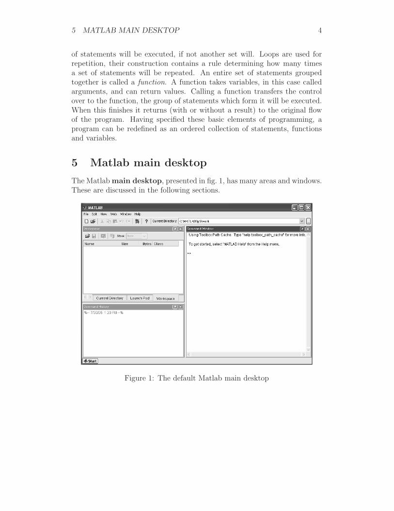
5 Matlab main desktop
The Matlab main desktop, presented in fig. 1, has many areas and windows.These are discussed in the following sections.
Figure 1: The default Matlab main desktop
5 MATLAB MAIN DESKTOP 5
5.1 Title bar
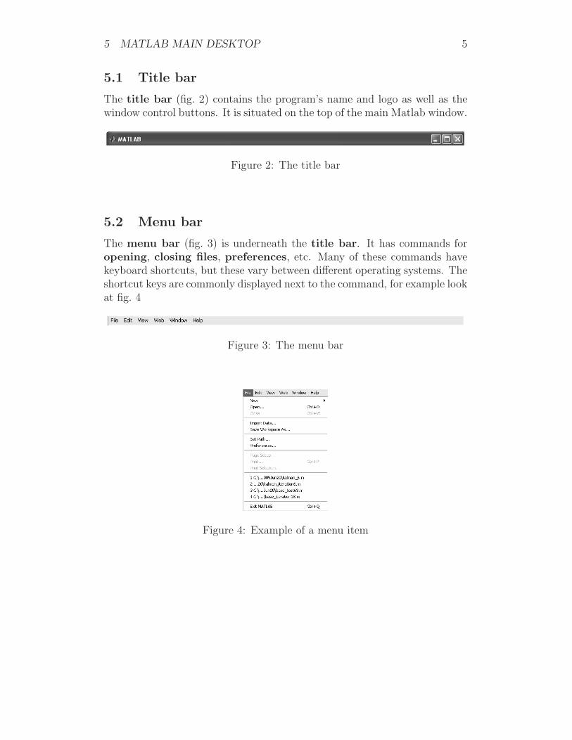
The title bar (fig. 2) contains the program’s name and logo as well as thewindow control buttons. It is situated on the top of the main Matlab window.
Figure 2: The title bar
5.2 Menu bar
The menu bar (fig. 3) is underneath the title bar. It has commands foropening, closing files, preferences, etc. Many of these commands havekeyboard shortcuts, but these vary between different operating systems. Theshortcut keys are commonly displayed next to the command, for example lookat fig. 4
Figure 3: The menu bar
Figure 4: Example of a menu item

5 MATLAB MAIN DESKTOP 6
5.3 Desktop toolbar
The desktop toolbar (fig. 5) is placed underneath the menu bar. It con-tains many items found on the menus, new file, open, copy, paste, ... .To find out what each icon does, leave the mouse above it for a few secondsand a small box with a tool tip will appear, e.g. fig. 6.
Figure 5: The desktop toolbar
Figure 6: A tooltip
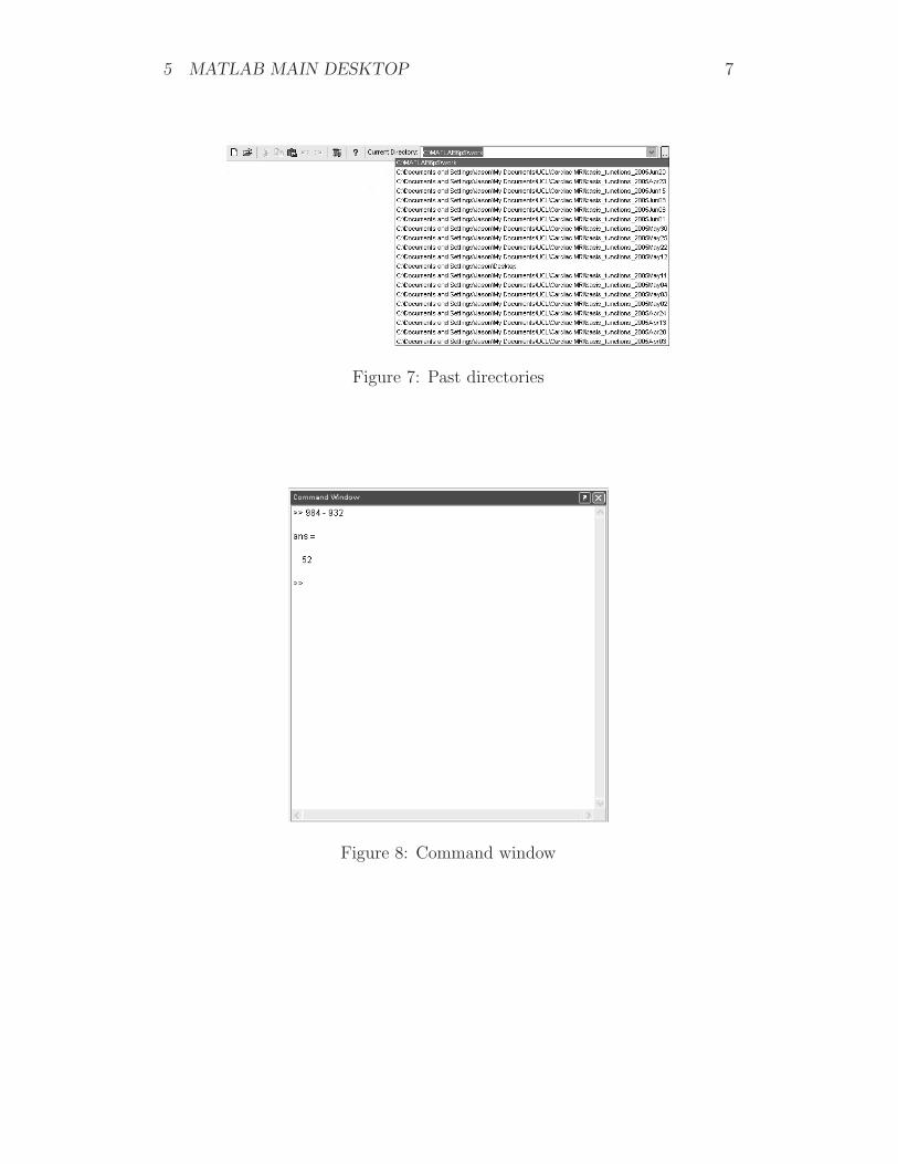
On the left side of the desktop toolbar there is box, which can be edited,called the current directory. This defines the location, where Matlab isworking. It is the folder at which the user is looking at. If Matlab (or theuser) can’t find a particular file, it means that the file is not in the currentdirectory. Commonly used or referenced directories can be setup from themenu bar using File → Set Path... . The small arrow on the right of thebox will show past current directories (fig. 7). Next to that the browse tool,the icon with the three dots, is used for finding a folder.
5.4 Command window
The command window (fig. 8) is the most important part of the Matlabmain desktop. It is the window where input and output appears. In thiswindow the user can enter commands and obtain results. Each new line onthe command prompt starts with the symbol >>. This defines where newinput can be entered. Input can be apart from Matlab commands, variousDOS or Linux prompt type of commands, e.g dir, ls.
5 MATLAB MAIN DESKTOP 7
Figure 7: Past directories
Figure 8: Command window
5 MATLAB MAIN DESKTOP 8
By pressing the up arrow on the keyboard the user can scroll throughall the previously entered commands. To scroll back the down arrow can beused. If a letter (or more) is typed, then the up and down arrows can beused to scroll through all the commands that have been previously typed andbegin with these letters. The tab button can be used to complete the nameof commands or functions. If a command does not exist or if more than onecommands with the same starting letters exist, then pressing the tab willmake a sound.
5.5 Command history
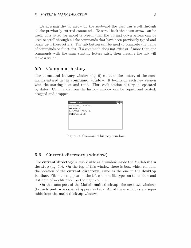
The command history window (fig. 9) contains the history of the com-mands entered in the command window. It begins on each new sessionwith the starting date and time. Thus each session history is separatedby dates. Commands from the history window can be copied and pasted,dragged and dropped.
Figure 9: Command history window
5.6 Current directory (window)
The current directory is also visible as a window inside the Matlab maindesktop (fig. 10). On the top of this window there is box, which containsthe location of the current directory, same as the one in the desktoptoolbar. File names appear on the left column, file types on the middle andlast date of modification on the right column.
On the same part of the Matlab main desktop, the next two windows(launch pad, workspace) appear as tabs. All of these windows are sepa-rable from the main desktop window.

5 MATLAB MAIN DESKTOP 9
Figure 10: Current directory window
5.7 Launch pad
The launch pad (fig. 11) is a way of accessing various Matlab resources,such as the import wizard, the profiler, the Graphical User Interface(GUI) builder, etc.
Figure 11: Launch pad
These windows appear as separate windows from the Matlab main desktop,some of which can be docked, that is they can be a part of the main desktop,and some which cannot be docked, they are called undockable windows.The launch pad can also be used to launch the help and demo files ofthe toolboxes. As it can be seen on fig. 11 it lives on the same window as the
6 OPENING AND EDITING FILES 10
current directory. Those two can be switched using the tabs on the lowestpart of the window, by pressing the one with the corresponding name.
5.8 Workspace
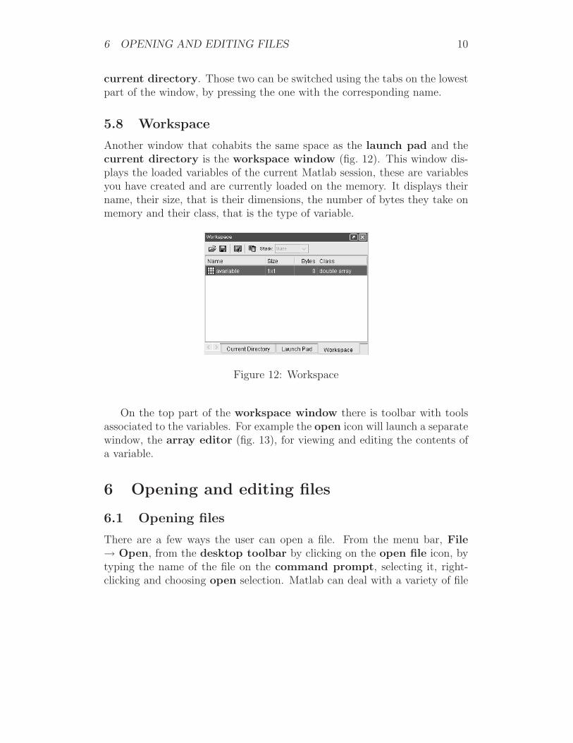
Another window that cohabits the same space as the launch pad and thecurrent directory is the workspace window (fig. 12). This window dis-plays the loaded variables of the current Matlab session, these are variablesyou have created and are currently loaded on the memory. It displays theirname, their size, that is their dimensions, the number of bytes they take onmemory and their class, that is the type of variable.
Figure 12: Workspace
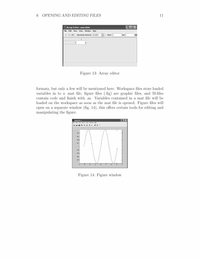
On the top part of the workspace window there is toolbar with toolsassociated to the variables. For example the open icon will launch a separatewindow, the array editor (fig. 13), for viewing and editing the contents ofa variable.
6 Opening and editing files
6.1 Opening files
There are a few ways the user can open a file. From the menu bar, File→ Open, from the desktop toolbar by clicking on the open file icon, bytyping the name of the file on the command prompt, selecting it, right-clicking and choosing open selection. Matlab can deal with a variety of file
6 OPENING AND EDITING FILES 11
Figure 13: Array editor
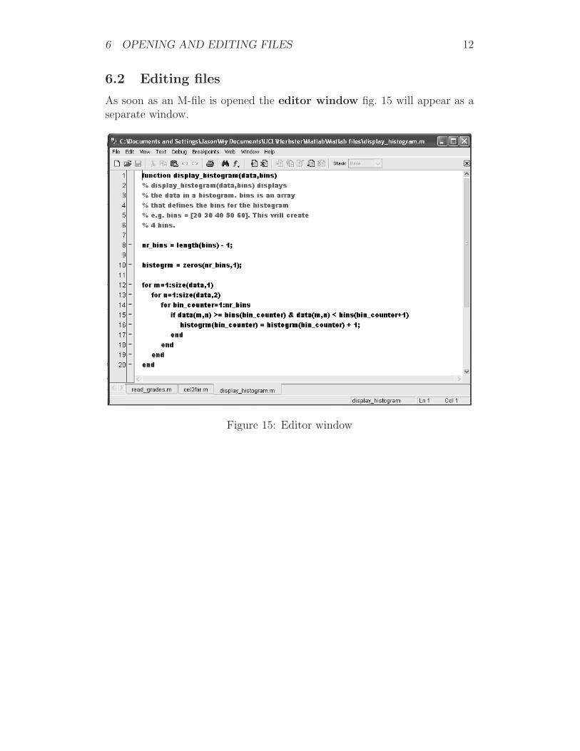
formats, but only a few will be mentioned here. Workspace files store loadedvariables in to a .mat file, figure files (.fig) are graphic files, and M-filescontain code and finish with .m. Variables contained in a mat file will beloaded on the workspace as soon as the mat file is opened. Figure files willopen on a separate window (fig. 14), this offers certain tools for editing andmanipulating the figure.
Figure 14: Figure window
6 OPENING AND EDITING FILES 12
6.2 Editing files
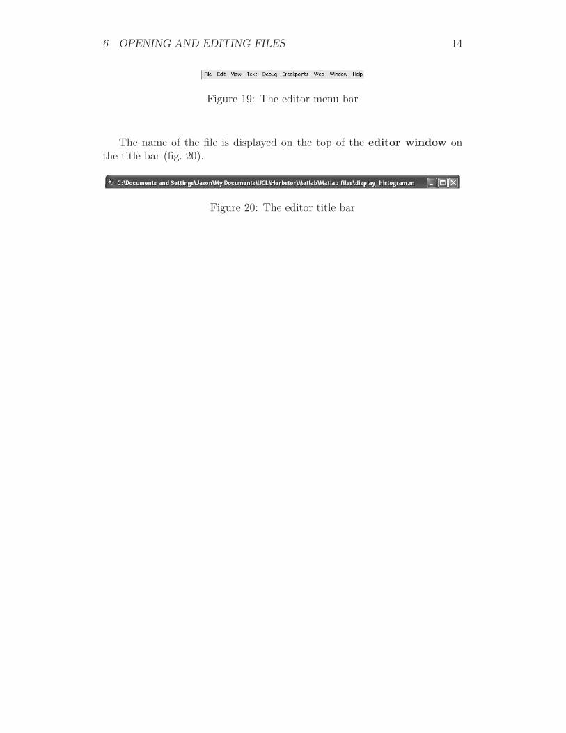
As soon as an M-file is opened the editor window fig. 15 will appear as aseparate window.
Figure 15: Editor window

6 OPENING AND EDITING FILES 13
This window can be docked in to the Matlab main desktop. Every file thatis opened will appear in the same window. Each file can be in its own editorwindow, in most cases it is practical to keep them in one. Files are chosenby the tabs on the lower part of the editor window (fig. 16).
Figure 16: Editor tabs
Of course one could use any editor, but Matlab’s editor offers color coding,running and debugging facilities. Similar to the command prompt, the usercan select the name of a function file, right-click on it and open it. On thebottom right of the editor window (fig. 17), information about the file isdisplayed as well as the line and the column where the cursor is placed, thiscan be very useful when debugging. On the left side of the editing area thelines are numbered.
Figure 17: Information on the lower part of the editor
A toolbar (fig. 18) is displayed on the top of the editor window. Thestandard buttons, New file, Open file, Save, Copy, Cut, Paste, Printare placed here. Next to them the binocular icon represents the find tool.This is used for searching the file for a particular keyword and replacing itif required. Further to the right are the debugging tools for setting andclearing breakpoints. The Run button is also situated on the right of thedebugging tools. This will execute the code contained in the active file.
Figure 18: The editor toolbar
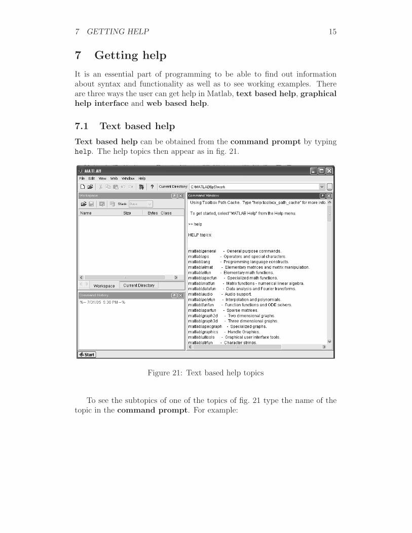
Files can also be executed using the menu bar (fig. 19) on the upperpart of the editor window in Debug → Run. The menu bar contains allof the toolbar commands and many others.
6 OPENING AND EDITING FILES 14
Figure 19: The editor menu bar
The name of the file is displayed on the top of the editor window onthe title bar (fig. 20).
Figure 20: The editor title bar
7 GETTING HELP 15
7 Getting help
It is an essential part of programming to be able to find out informationabout syntax and functionality as well as to see working examples. Thereare three ways the user can get help in Matlab, text based help, graphicalhelp interface and web based help.
7.1 Text based help
Text based help can be obtained from the command prompt by typinghelp. The help topics then appear as in fig. 21.
Figure 21: Text based help topics
To see the subtopics of one of the topics of fig. 21 type the name of thetopic in the command prompt. For example:

7 GETTING HELP 16
>> help matlab\general
The command help can also be used to find out information about a specificfunction. For example:
>> help sin
SIN Sine.
SIN(X) is the sine of the elements of X.
Overloaded methods
help sym/sin.m
In the case the function is unknown or the user wants to search for aspecific keyword, the command lookfor can be used.
>> lookfor infinity
INF Infinity.
CEIL Round towards plus infinity.
FLOOR Round towards minus infinity.
CHOLINC Sparse Incomplete Cholesky and Cholesky-Infinity factorizations.
ACTDEMO Demo of digital H-infinity hydraulic actuator design.
DHINF Discrete H-Infinity control synthesis (bilinear transform version).
DHINFOPT Discrete H-Infinity control synthesis via Gamma iteration.
DINTDEMO Demo of H-Infinity design of double integrator plant.
...
The command lookfor will search in all help entries. To find out the detailsin one of the search results help can be used as previously:
>> help INF
INF Infinity.
INF returns the IEEE arithmetic representation for positive
infinity. Infinity is also produced by operations like dividing by
zero, eg. 1.0/0.0, or from overflow, eg. exp(1000).
See also NaN, ISFINITE, ISINF.

7 GETTING HELP 17
7.2 Graphical interface help
A more extensive and user friendly option to get help is the graphical in-terface help window (fig. 22). This is a separate window and it is launchedfrom the menu bar, Help → Matlab help, the main desktop toolbarby pressing the question mark or by typing helpbrowser in the commandprompt.
Figure 22: Help browser
The help browser has a menu bar on the top and it is divided into twomain areas. The area on the left is query area and the right one is whereinformation appears.
On the top of the information area (fig. 23) there is small toolbar withback, forward and reload buttons, similar to a web browser, a print buttonand a Find in page button for searching a keyword in the current page.

7 GETTING HELP 18
Figure 23: Information area
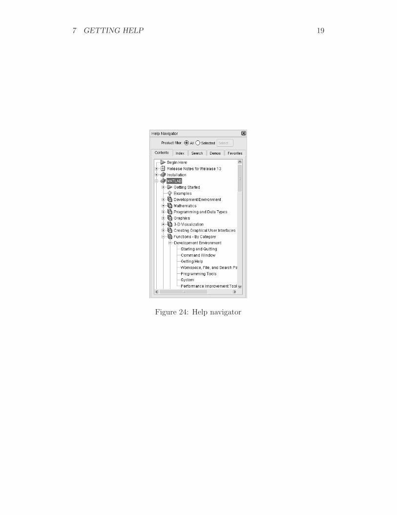
The query area on the left, also called the help navigator (fig. 24) hasfive tabs, Contents, Index, Search, Demos and Favorites.
7 GETTING HELP 19
Figure 24: Help navigator
7 GETTING HELP 20
The Contents tab, shown in fig. 24, has a tree list of all the help informationin Matlab. By clicking on a particular item, the information appears on theright area.
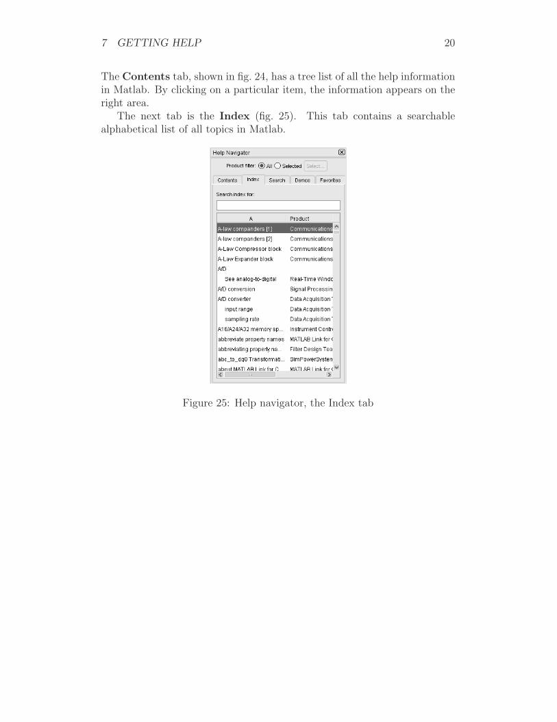
The next tab is the Index (fig. 25). This tab contains a searchablealphabetical list of all topics in Matlab.
Figure 25: Help navigator, the Index tab
7 GETTING HELP 21
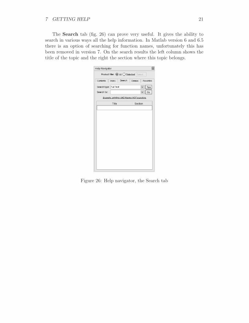
The Search tab (fig. 26) can prove very useful. It gives the ability tosearch in various ways all the help information. In Matlab version 6 and 6.5there is an option of searching for function names, unfortunately this hasbeen removed in version 7. On the search results the left column shows thetitle of the topic and the right the section where this topic belongs.
Figure 26: Help navigator, the Search tab
7 GETTING HELP 22
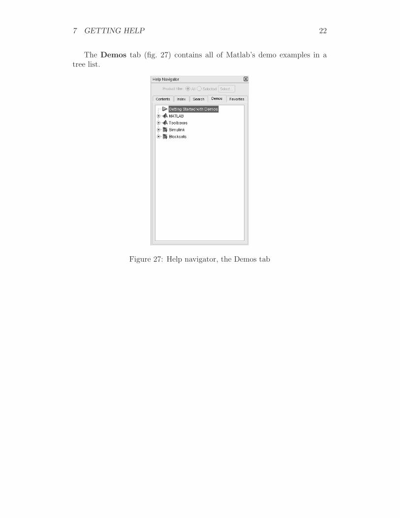
The Demos tab (fig. 27) contains all of Matlab’s demo examples in atree list.
Figure 27: Help navigator, the Demos tab
7 GETTING HELP 23
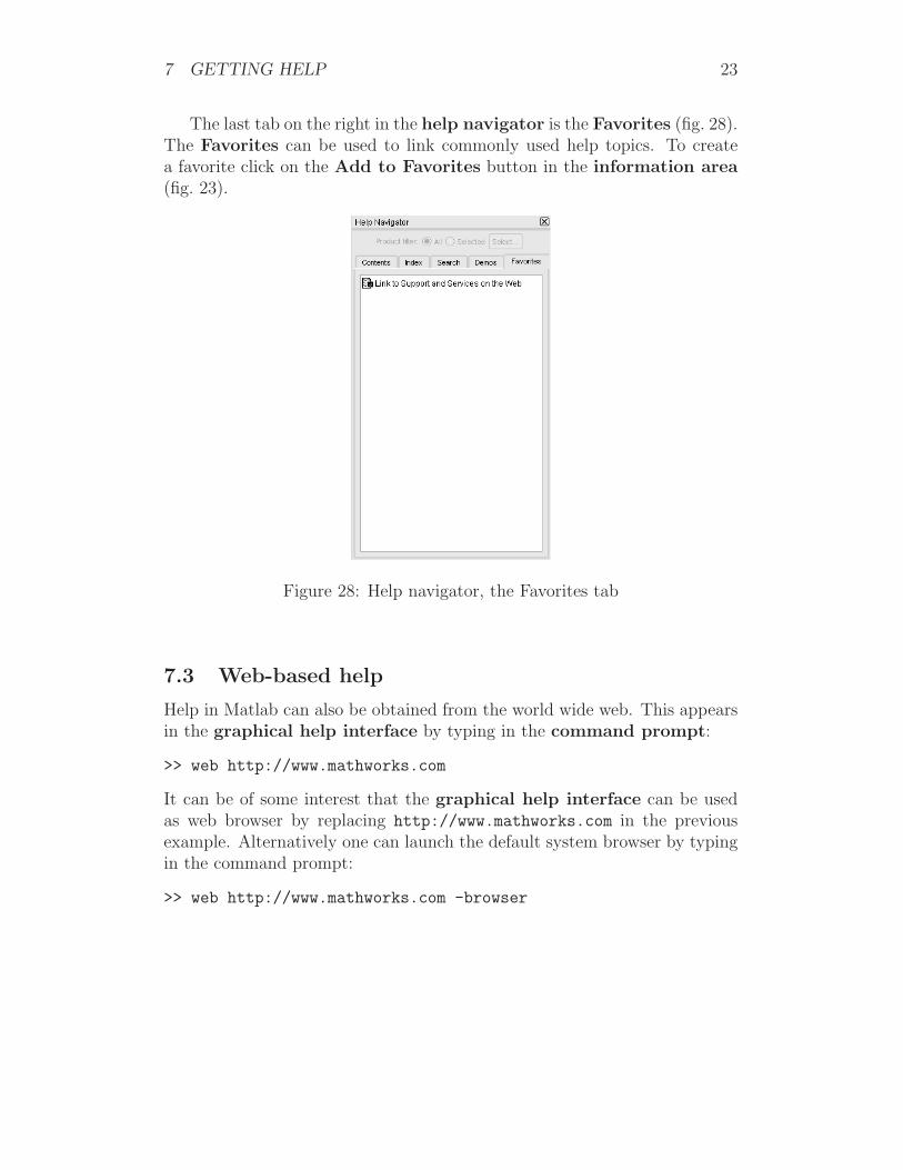
The last tab on the right in the help navigator is the Favorites (fig. 28).The Favorites can be used to link commonly used help topics. To createa favorite click on the Add to Favorites button in the information area(fig. 23).
Figure 28: Help navigator, the Favorites tab
7.3 Web-based help
Help in Matlab can also be obtained from the world wide web. This appearsin the graphical help interface by typing in the command prompt:
>> web http://www.mathworks.com
It can be of some interest that the graphical help interface can be usedas web browser by replacing http://www.mathworks.com in the previousexample. Alternatively one can launch the default system browser by typingin the command prompt:
>> web http://www.mathworks.com -browser
8 SETTING THE DESKTOP LAYOUT 24
8 Setting the desktop layout
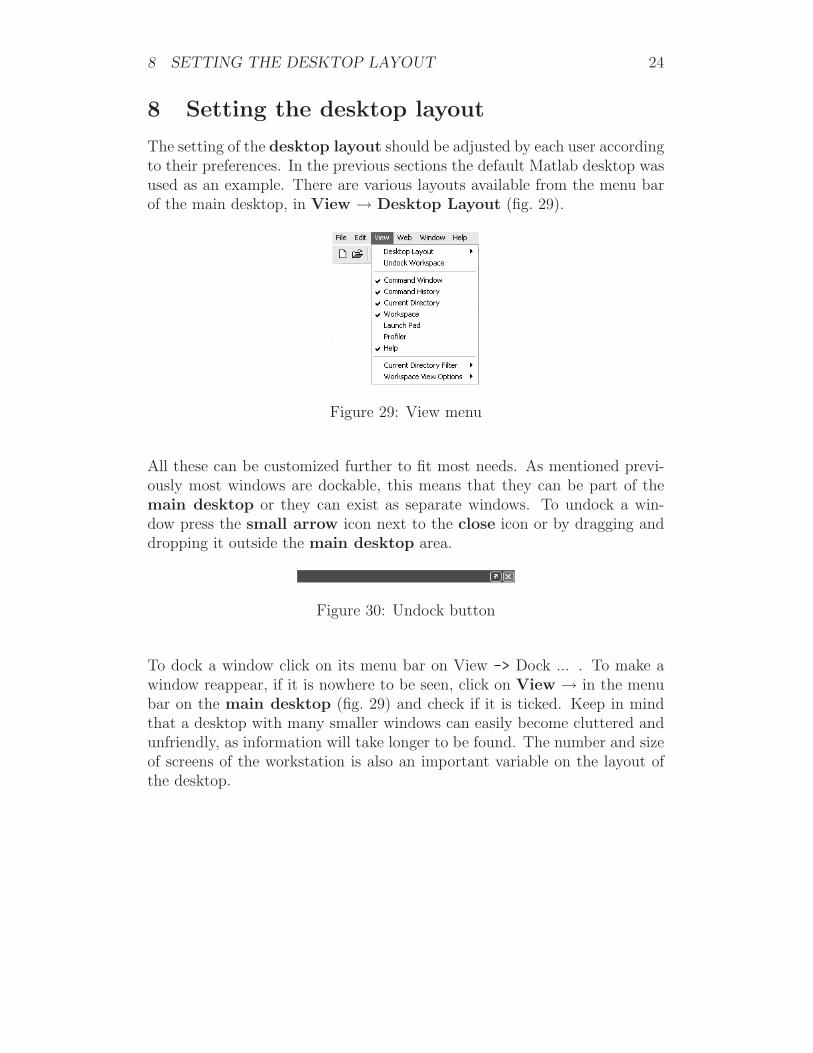
The setting of the desktop layout should be adjusted by each user accordingto their preferences. In the previous sections the default Matlab desktop wasused as an example. There are various layouts available from the menu barof the main desktop, in View → Desktop Layout (fig. 29).
Figure 29: View menu
All these can be customized further to fit most needs. As mentioned previ-ously most windows are dockable, this means that they can be part of themain desktop or they can exist as separate windows. To undock a win-dow press the small arrow icon next to the close icon or by dragging anddropping it outside the main desktop area.
Figure 30: Undock button
To dock a window click on its menu bar on View -> Dock ... . To make awindow reappear, if it is nowhere to be seen, click on View → in the menubar on the main desktop (fig. 29) and check if it is ticked. Keep in mindthat a desktop with many smaller windows can easily become cluttered andunfriendly, as information will take longer to be found. The number and sizeof screens of the workstation is also an important variable on the layout ofthe desktop.

25
Part II
Lecture 1
9 Overview of Lecture 1
• Style of notes
• Recommended reading
• Introduction to Matlab
• Building matrices
• Addressing and assigning elements
• Building special matrices
• Matrix operations
• Equation solving
• User defined functions
• Plotting
• Utility commands
• Summary table of functions

10 STYLE OF NOTES 26
10 Style of notes
These notes have been prepared to be compatible with Matlab version 6.5,for most cases this should be true for previous versions of Matlab as wellas version 7. Matlab version 7 offers new features, some of those will beexplained in comparison with version 6.5. It will be clearly stated, when afeature from version 7 is used.
The verbatim font is used for everything that is written in the Matlabprogramming language. For the names of variables we use small fonts forscalars, vectors and strings and capital fonts for matrices. Throughout thesenotes we will see examples that perform the same operation. This is intendedto present some of the different ways we can work in Matlab. At the endof each set of notes we have provided a summary table of all newly intro-duced functions with their corresponding page numbers. Many of Matlab’sfunctions introduced can take a different number of arguments, we have onlyincluded the basic arguments each function can take. For more details, youshould look in Matlab’s help.
11 Recommended reading
Matlab’s help contains all the built in functions with extensive details andexamples. These are well written and always worth looking at. More detailsand examples can be found in:
Hanselman, Duane C.: Mastering MATLAB 6 : a comprehensive tutorialand reference, Pearson Education
Kuncicky, David C.: Matlab programming, Pearson EducationFree alternatives similar to Matlab areScilab
http://www-rocq.inria.fr/scilab/Rlab
http://rlab.sourceforge.net/Octave
http://www.octave.org/
12 INTRODUCTION TO MATLAB 27
12 Introduction to Matlab
MATrix LABoratory is one of the most popular packages for scientific com-puting. It offers extensive libraries of numerical methods and a variety oftools for visualization. It is designed mainly for discrete computations withfocus on matrices. Even though it has the capability to perform analyticaltasks such as finding the derivative of a continuous function, it is not veryextensive on symbolic mathematics. A more suited tool for this job is an-other mathematical programming package called Mathematica, developed byStephen Wolfram.
Matlab is an interpreted programming language. The statements aretranslated in to machine code one by one by Matlab’s interpreter. In com-parison, a compiled programming language like C has a program translatedas a whole in to machine code by the compiler. Interpreted languages arefaster for development as they have no need for compilation and errors in thecode can be found quickly. To run a piece of Matlab code on any computerit has to have Matlab installed. In the case of compiled languages there is nosuch requirement. Because of the interpretation Matlab tends to be slowerthan compiled languages.
There are 3 ways in which you can work in Matlab, from the commandprompt of Matlab, writing scripts and writing functions. Matlab script andfunction files are called M-files. A script file takes no arguments, it is justa series of statements that will be executed sequentially. A function file cantake and return arguments. To begin with, we will start with writing directlyto the command prompt.
13 Building matrices
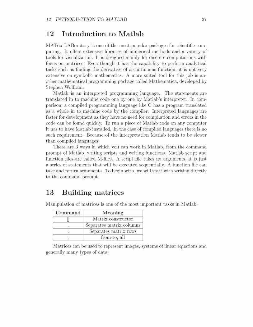
Manipulation of matrices is one of the most important tasks in Matlab.
Command Meaning[] Matrix constructor, Separates matrix columns; Separates matrix rows: from-to, all
Matrices can be used to represent images, systems of linear equations andgenerally many types of data.
13 BUILDING MATRICES 28
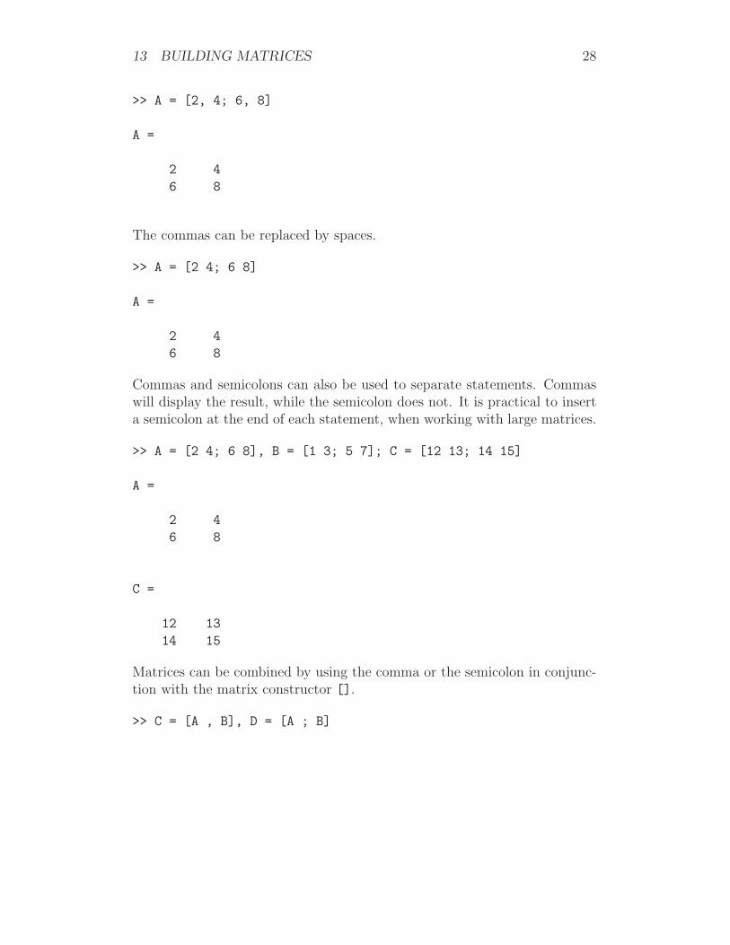
>> A = [2, 4; 6, 8]
A =
2 4
6 8
The commas can be replaced by spaces.
>> A = [2 4; 6 8]
A =
2 4
6 8
Commas and semicolons can also be used to separate statements. Commaswill display the result, while the semicolon does not. It is practical to inserta semicolon at the end of each statement, when working with large matrices.
>> A = [2 4; 6 8], B = [1 3; 5 7]; C = [12 13; 14 15]
A =
2 4
6 8
C =
12 13
14 15
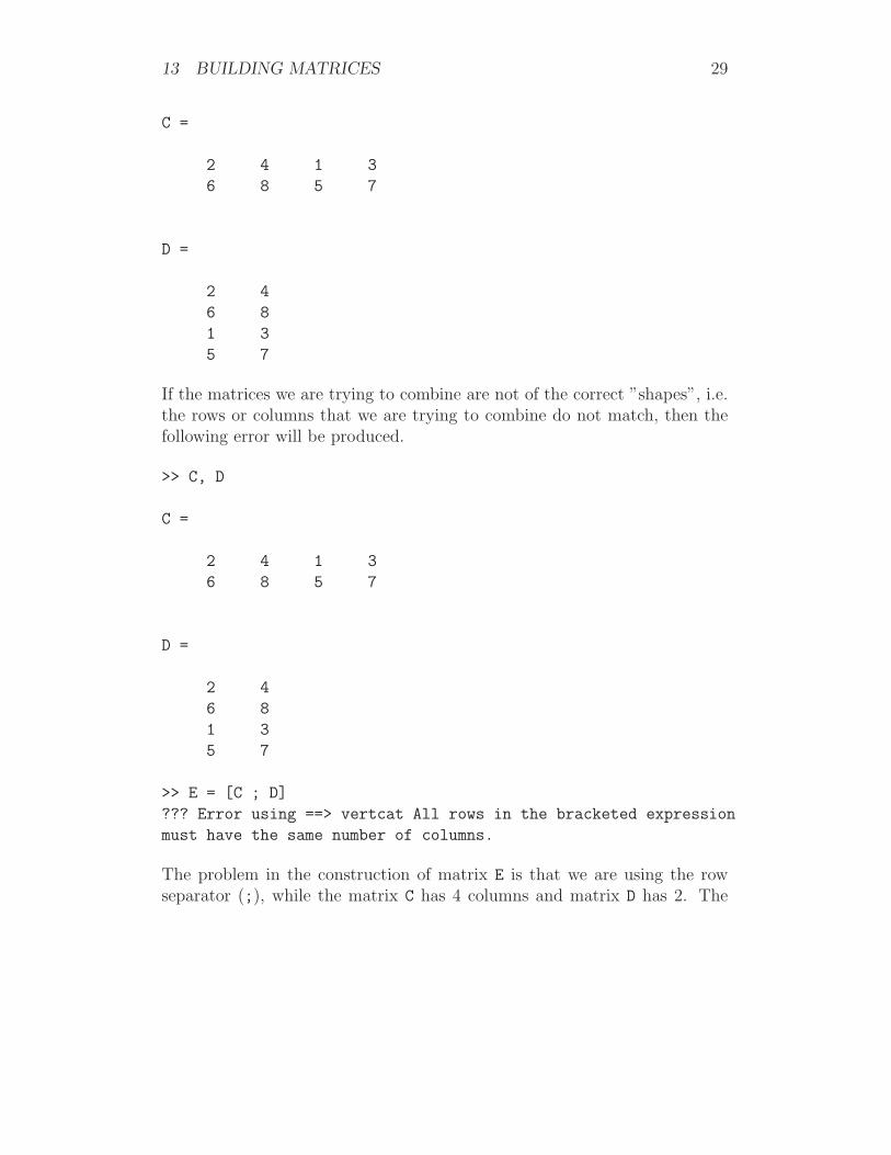
Matrices can be combined by using the comma or the semicolon in conjunc-tion with the matrix constructor [].
>> C = [A , B], D = [A ; B]
13 BUILDING MATRICES 29
C =
2 4 1 3
6 8 5 7
D =
2 4
6 8
1 3
5 7
If the matrices we are trying to combine are not of the correct ”shapes”, i.e.the rows or columns that we are trying to combine do not match, then thefollowing error will be produced.
>> C, D
C =
2 4 1 3
6 8 5 7
D =
2 4
6 8
1 3
5 7
>> E = [C ; D]
??? Error using ==> vertcat All rows in the bracketed expression
must have the same number of columns.
The problem in the construction of matrix E is that we are using the rowseparator (;), while the matrix C has 4 columns and matrix D has 2. The
13 BUILDING MATRICES 30
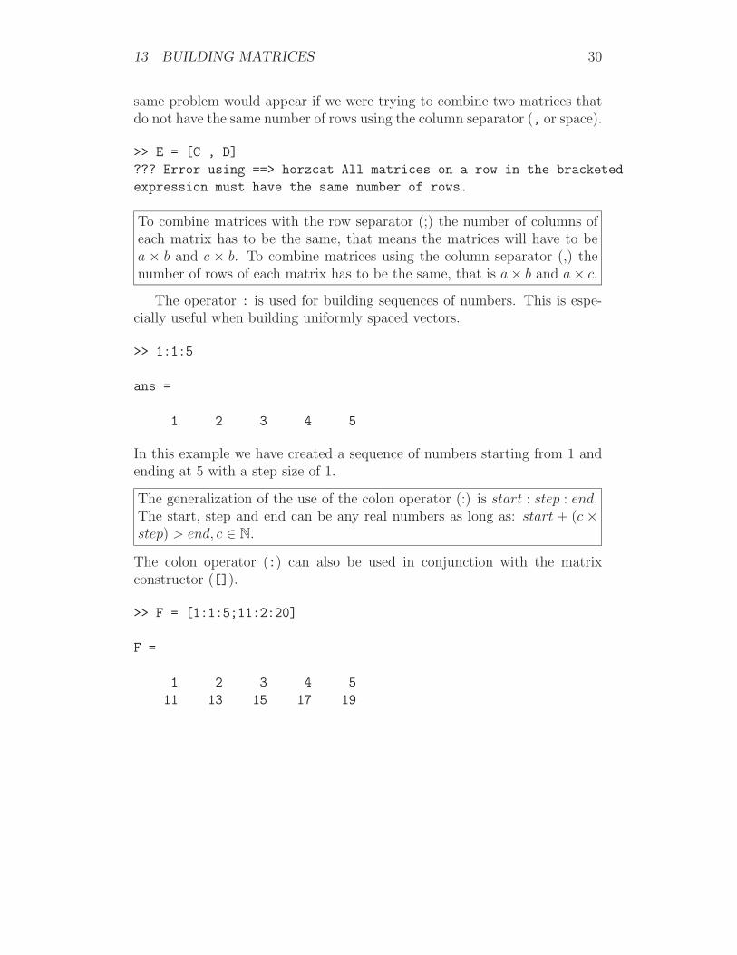
same problem would appear if we were trying to combine two matrices thatdo not have the same number of rows using the column separator (, or space).
>> E = [C , D]
??? Error using ==> horzcat All matrices on a row in the bracketed
expression must have the same number of rows.
To combine matrices with the row separator (;) the number of columns ofeach matrix has to be the same, that means the matrices will have to bea × b and c × b. To combine matrices using the column separator (,) thenumber of rows of each matrix has to be the same, that is a × b and a × c.
The operator : is used for building sequences of numbers. This is espe-cially useful when building uniformly spaced vectors.
>> 1:1:5
ans =
1 2 3 4 5
In this example we have created a sequence of numbers starting from 1 andending at 5 with a step size of 1.
The generalization of the use of the colon operator (:) is start : step : end.The start, step and end can be any real numbers as long as: start + (c ×step) > end, c ∈ N.
The colon operator (:) can also be used in conjunction with the matrixconstructor ([]).
>> F = [1:1:5;11:2:20]
F =
1 2 3 4 5
11 13 15 17 19

14 ADDRESSING AND ASSIGNING ELEMENTS 31
14 Addressing and assigning elements
The first action we have to take in order to assign a value to a variable isto address the element of the variable we want. To address an element ofa matrix the round brackets (a,b) are used. a and b are positive integers,i.e. a, b ∈ N. The first element inside the brackets denotes the row and thesecond denotes the column.
>> F
F =
1 2 3 4 5
11 13 15 17 19
>> F(2,3)
ans =
15
Vectors can also be used to address elements in a matrix.
>> F([1 ; 2] , 3)
ans =
3
15
>> F([1 2] , 3)
ans =
3
15
The colon : can be used to address all the elements of a row or column.

14 ADDRESSING AND ASSIGNING ELEMENTS 32
>> F(:,1)
ans =
1
11
>> F(1,:)
ans =
1 2 3 4 5
Matrices can also be addressed as if they were a vector. The elements arenumbered by first counting the elements of a column and then progressingto the next column (as in fig. 31).
Figure 31: Numbering of a matrix as a vector
>> F
F =
1 2 3 4 5
11 13 15 17 19
>> F(3)
ans =
2
14 ADDRESSING AND ASSIGNING ELEMENTS 33
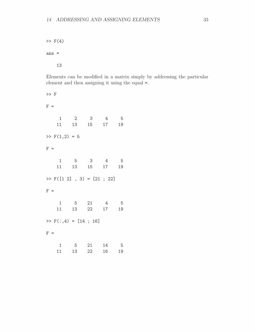
>> F(4)
ans =
13
Elements can be modified in a matrix simply by addressing the particularelement and then assigning it using the equal =.
>> F
F =
1 2 3 4 5
11 13 15 17 19
>> F(1,2) = 5
F =
1 5 3 4 5
11 13 15 17 19
>> F([1 2] , 3) = [21 ; 22]
F =
1 5 21 4 5
11 13 22 17 19
>> F(:,4) = [14 ; 16]
F =
1 5 21 14 5
11 13 22 16 19
15 BUILDING SPECIAL MATRICES 34
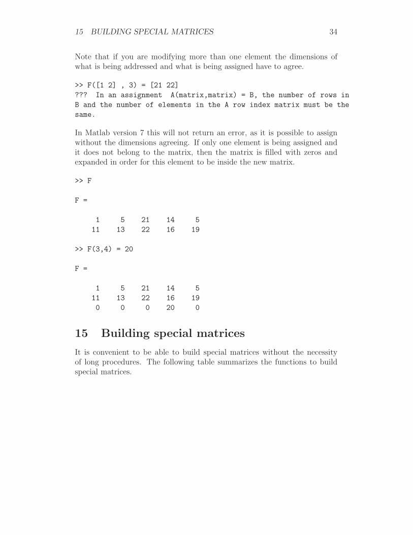
Note that if you are modifying more than one element the dimensions ofwhat is being addressed and what is being assigned have to agree.
>> F([1 2] , 3) = [21 22]
??? In an assignment A(matrix,matrix) = B, the number of rows in
B and the number of elements in the A row index matrix must be the
same.
In Matlab version 7 this will not return an error, as it is possible to assignwithout the dimensions agreeing. If only one element is being assigned andit does not belong to the matrix, then the matrix is filled with zeros andexpanded in order for this element to be inside the new matrix.
>> F
F =
1 5 21 14 5
11 13 22 16 19
>> F(3,4) = 20
F =
1 5 21 14 5
11 13 22 16 19
0 0 0 20 0
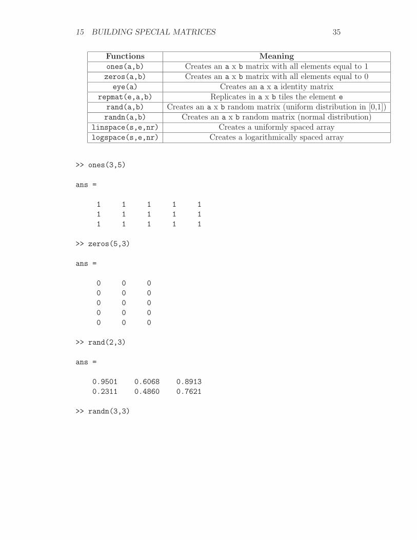
15 Building special matrices
It is convenient to be able to build special matrices without the necessityof long procedures. The following table summarizes the functions to buildspecial matrices.
15 BUILDING SPECIAL MATRICES 35
Functions Meaningones(a,b) Creates an a x b matrix with all elements equal to 1zeros(a,b) Creates an a x b matrix with all elements equal to 0
eye(a) Creates an a x a identity matrixrepmat(e,a,b) Replicates in a x b tiles the element e
rand(a,b) Creates an a x b random matrix (uniform distribution in [0,1])randn(a,b) Creates an a x b random matrix (normal distribution)
linspace(s,e,nr) Creates a uniformly spaced arraylogspace(s,e,nr) Creates a logarithmically spaced array
>> ones(3,5)
ans =
1 1 1 1 1
1 1 1 1 1
1 1 1 1 1
>> zeros(5,3)
ans =
0 0 0
0 0 0
0 0 0
0 0 0
0 0 0
>> rand(2,3)
ans =
0.9501 0.6068 0.8913
0.2311 0.4860 0.7621
>> randn(3,3)

15 BUILDING SPECIAL MATRICES 36
ans =
1.1892 0.1746 -0.5883
-0.0376 -0.1867 2.1832
0.3273 0.7258 -0.1364
The functions ones(), zeros(), rand(), randn() can be simplified forsquare matrices by only having one number inside the round brackets.
>> ones(3)
ans =
1 1 1
1 1 1
1 1 1
>> zeros(3)
ans =
0 0 0
0 0 0
0 0 0
>> randn(3)
ans =
-0.0592 0.5077 -0.6436
-1.0106 1.6924 0.3803
0.6145 0.5913 -1.0091
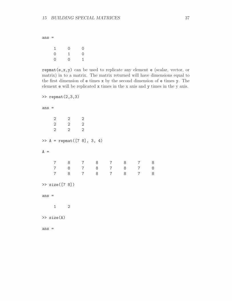
The function eye(a) constructs the identity matrix, which is by definitionsquare. The identity matrix has 1 in the elements on the diagonal and 0everywhere else.
>> eye(3)
15 BUILDING SPECIAL MATRICES 37
ans =
1 0 0
0 1 0
0 0 1
repmat(e,x,y) can be used to replicate any element e (scalar, vector, ormatrix) in to a matrix. The matrix returned will have dimensions equal tothe first dimension of e times x by the second dimension of e times y. Theelement e will be replicated x times in the x axis and y times in the y axis.
>> repmat(2,3,3)
ans =
2 2 2
2 2 2
2 2 2
>> A = repmat([7 8], 3, 4)
A =
7 8 7 8 7 8 7 8
7 8 7 8 7 8 7 8
7 8 7 8 7 8 7 8
>> size([7 8])
ans =
1 2
>> size(A)
ans =

15 BUILDING SPECIAL MATRICES 38
3 8
>> repmat([1 2],3,3)
ans =
1 2 1 2 1 2
1 2 1 2 1 2
1 2 1 2 1 2
>> repmat([1; 2],3,3)
ans =
1 1 1
2 2 2
1 1 1
2 2 2
1 1 1
2 2 2
>> repmat([1 3; 2 4],3,3)
ans =
1 3 1 3 1 3
2 4 2 4 2 4
1 3 1 3 1 3
2 4 2 4 2 4
1 3 1 3 1 3
2 4 2 4 2 4
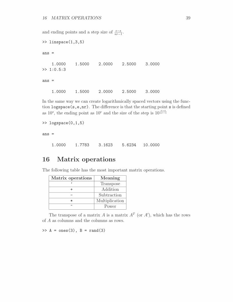
The function size(A) returns the number of rows and columns of A. To createuniformly spaced vectors, the function linspace(s,e,nr) can be used. Thefirst argument (s) inside the round brackets is the starting point, the second(e) is the end point and the third one (nr) is the number of elements includingthe starting and the end point. An equivalent operation can be performedusing the colon : notation, as discussed previously, with the same starting
16 MATRIX OPERATIONS 39
and ending points and a step size of e−snr−1
.
>> linspace(1,3,5)
ans =
1.0000 1.5000 2.0000 2.5000 3.0000
>> 1:0.5:3
ans =
1.0000 1.5000 2.0000 2.5000 3.0000
In the same way we can create logarithmically spaced vectors using the func-tion logspace(s,e,nr). The difference is that the starting point s is defined
as 10s, the ending point as 10e and the size of the step is 10e−s
nr−1
>> logspace(0,1,5)
ans =
1.0000 1.7783 3.1623 5.6234 10.0000
16 Matrix operations
The following table has the most important matrix operations.
Matrix operations Meaning’ Transpose+ Addition- Subtraction* Multiplication^ Power
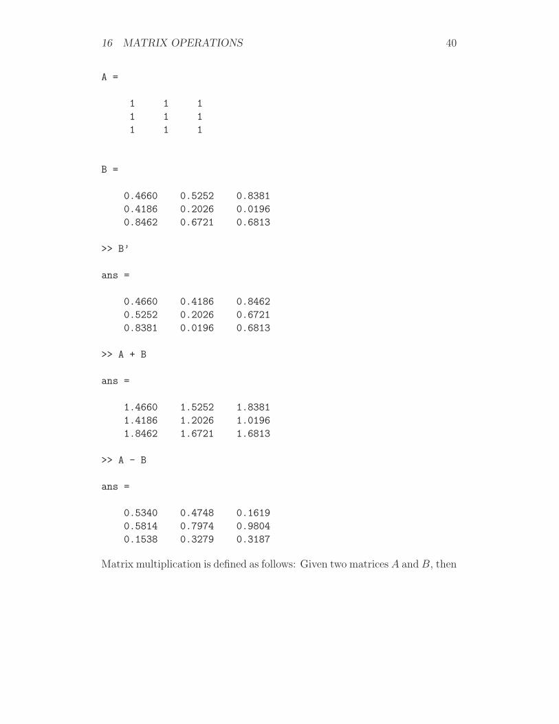
The transpose of a matrix A is a matrix AT (or A′), which has the rowsof A as columns and the columns as rows.
>> A = ones(3), B = rand(3)
16 MATRIX OPERATIONS 40
A =
1 1 1
1 1 1
1 1 1
B =
0.4660 0.5252 0.8381
0.4186 0.2026 0.0196
0.8462 0.6721 0.6813
>> B’
ans =
0.4660 0.4186 0.8462
0.5252 0.2026 0.6721
0.8381 0.0196 0.6813
>> A + B
ans =
1.4660 1.5252 1.8381
1.4186 1.2026 1.0196
1.8462 1.6721 1.6813
>> A - B
ans =
0.5340 0.4748 0.1619
0.5814 0.7974 0.9804
0.1538 0.3279 0.3187
Matrix multiplication is defined as follows: Given two matrices A and B, then

16 MATRIX OPERATIONS 41
their product C = AB is Crt = ArsBst and an element of matrix C is definedas cij =
∑s
k=1 aikbkj, where aik, bkj are elements of A and B respectively.
>> A * B
ans =
1.7309 1.3999 1.5390
1.7309 1.3999 1.5390
1.7309 1.3999 1.5390
Power of matrix is defined as follows: Ak = A × A...A︸ ︷︷ ︸
k times
>> B^2
ans =
1.1462 0.9145 0.9719
0.2965 0.2741 0.3682
1.2522 1.0385 1.1866
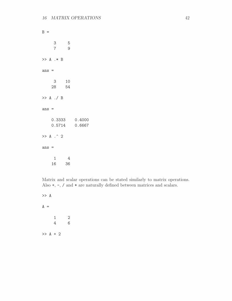
Vectorized operations are also useful. These operations are performed be-tween two corresponding elements of the two matrices. The following tablecontains a list of main operations.
Vectorized operations Meaning.* Multiply corresponding elements./ Divide corresponding elements.^ Power of each element
>> A = [1 2; 4 6], B = [3 5; 7 9]
A =
1 2
4 6
16 MATRIX OPERATIONS 42
B =
3 5
7 9
>> A .* B
ans =
3 10
28 54
>> A ./ B
ans =
0.3333 0.4000
0.5714 0.6667
>> A .^ 2
ans =
1 4
16 36
Matrix and scalar operations can be stated similarly to matrix operations.Also +, -, / and * are naturally defined between matrices and scalars.
>> A
A =
1 2
4 6
>> A + 2

17 EQUATION SOLVING 43
ans =
3 4
6 8
>> A - 2
ans =
-1 0
2 4
>> A * 2
ans =
2 4
8 12
>> A / 2
ans =
0.5000 1.0000
2.0000 3.0000
17 Equation solving
Consider the following system of equations.
2x1 + x2 − 2x3 = 10 (1)
6x1 + 4x2 + 4x3 = 2
10x1 + 8x2 + 6x3 = 8
This can be represented by a matrix equation Ax = b
17 EQUATION SOLVING 44
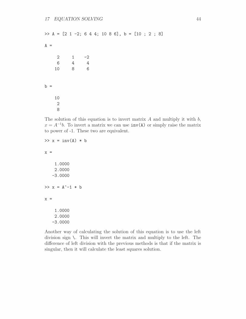
>> A = [2 1 -2; 6 4 4; 10 8 6], b = [10 ; 2 ; 8]
A =
2 1 -2
6 4 4
10 8 6
b =
10
2
8
The solution of this equation is to invert matrix A and multiply it with b,x = A−1b. To invert a matrix we can use inv(A) or simply raise the matrixto power of -1. These two are equivalent.
>> x = inv(A) * b
x =
1.0000
2.0000
-3.0000
>> x = A^-1 * b
x =
1.0000
2.0000
-3.0000
Another way of calculating the solution of this equation is to use the leftdivision sign \. This will invert the matrix and multiply to the left. Thedifference of left division with the previous methods is that if the matrix issingular, then it will calculate the least squares solution.
18 USER DEFINED FUNCTIONS 45
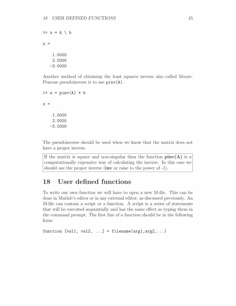
>> x = A \ b
x =
1.0000
2.0000
-3.0000
Another method of obtaining the least squares inverse also called Moore-Penrose pseudoinverse is to use pinv(A).
>> x = pinv(A) * b
x =
1.0000
2.0000
-3.0000
The pseudoinverse should be used when we know that the matrix does nothave a proper inverse.
If the matrix is square and non-singular then the function pinv(A) is acomputationally expensive way of calculating the inverse. In this case weshould use the proper inverse (inv or raise to the power of -1).
18 User defined functions
To write our own function we will have to open a new M-file. This can bedone in Matlab’s editor or in any external editor, as discussed previously. AnM-file can contain a script or a function. A script is a series of statementsthat will be executed sequentially and has the same effect as typing them inthe command prompt. The first line of a function should be in the followingform:
function [val1, val2, ...] = filename(arg1,arg2,...)

18 USER DEFINED FUNCTIONS 46
Note that the name of the function has to match the name of the file. The firstcommented lines after the first line, which defines the function, are displayedwhen requesting Matlab’s help. Create a function called my_function withthe following code.
function [rtn] = my_function(a,b)
% rtn = my_function(a,b) takes two variables and adds them
rtn = a + b;
>> my_function(2,4)
ans =
6
>> help my_function
rtn = my_function(a,b) takes two variables and adds them
Using the first lines for information on the function, explaining what thefunction does, what arguments it takes, what variables it returns, versionnumber, etc. can prove to be very useful in large projects.
Remember that all variables inside a function are local and cannot be ac-cessed from the command prompt or any other functions. All variablesinside a script file can be accessed from the command prompt and otherscripts.
Next is an example of a function myint that integrates a given function f onan closed interval [a,b] according to accuracy n. The higher n is the moresamples myint will take in the interval [a,b] for the function f.
function s = myint(f,a,b,n)
% function s = myint(’f’,a,b,n)
%
% This function numerically integrates f from a to b
% by summing n approximating rectangles
invs = linspace(a,b,n+1) ;
fx = feval(f,invs(1:n)) ;
s =((b-a)/n)*sum(fx) ;
19 PLOTTING 47
On the command prompt we can type:
>> myint(’sin’,0,pi,100)
ans =
1.9998
The function feval(f,values) takes a string f defining the function andan array values with the values of where the function f should be evalu-ated. feval can take any predefined, both user created and built in Matlab,function as the f argument.
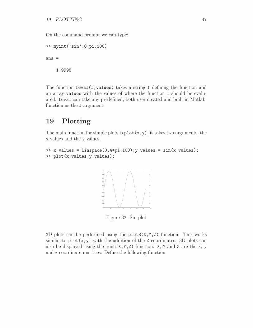
19 Plotting
The main function for simple plots is plot(x,y), it takes two arguments, thex values and the y values.
>> x_values = linspace(0,4*pi,100);y_values = sin(x_values);
>> plot(x_values,y_values);
0 2 4 6 8 10 12 14−1
−0.8
−0.6
−0.4
−0.2
0
0.2
0.4
0.6
0.8
1
Figure 32: Sin plot
3D plots can be performed using the plot3(X,Y,Z) function. This workssimilar to plot(x,y) with the addition of the Z coordinates. 3D plots canalso be displayed using the mesh(X,Y,Z) function. X, Y and Z are the x, yand z coordinate matrices. Define the following function:
19 PLOTTING 48
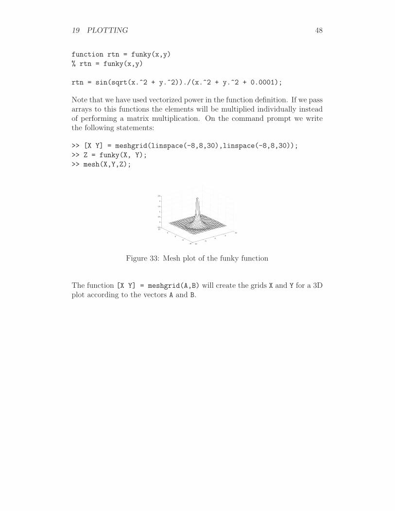
function rtn = funky(x,y)
% rtn = funky(x,y)
rtn = sin(sqrt(x.^2 + y.^2))./(x.^2 + y.^2 + 0.0001);
Note that we have used vectorized power in the function definition. If we passarrays to this functions the elements will be multiplied individually insteadof performing a matrix multiplication. On the command prompt we writethe following statements:
>> [X Y] = meshgrid(linspace(-8,8,30),linspace(-8,8,30));
>> Z = funky(X, Y);
>> mesh(X,Y,Z);
−10
−5
0
5
10
−10
−5
0
5
10−0.5
0
0.5
1
1.5
2
2.5
Figure 33: Mesh plot of the funky function
The function [X Y] = meshgrid(A,B) will create the grids X and Y for a 3Dplot according to the vectors A and B.

20 UTILITY COMMANDS 49
20 Utility commands
Command Meaningwhos Gives the sizes and types of all loaded variables
save ’my_work’ Save the current workspace on to ’my_work’
load ’my_work’ Load ’my_work’ on to the current workspacediary on Starts diarydiary off Stops diaryclose all Closes all figure windowsclear all Clears from memory all loaded variables
clc Clear command windowControl + c Stops execution of a programControl + i Smart indent selected textControl + r Comment selected textControl + t Uncomment selected text
quit Exit Matlab

21 SUMMARY TABLE OF FUNCTIONS 50
21 Summary table of functions
Function p. Meaning[] 27 Matrix constructor, 27 Separates matrix columns; 27 Separates matrix rows: 27 from-to, all() 31 Addressing elements in matrix
ones(a,b) 35 Creates an a x b matrix with all elements equal to 1zeros(a,b) 35 Creates an a x b matrix with all elements equal to 0
eye(a) 35 Creates an a x b identity matrixrepmat(A,a,b) 35 Replicates in a x b tiles the element A
rand(a,b) 35 Creates an a x b random matrix (uniform distribution in [0,1])randn(a,b) 35 Creates an a x b random matrix (normal distribution)
linspace(s,e,nr) 35 Creates a uniformly spaced arraylogspace(s,e,nr) 35 Creates a logarithmically spaced array
size(A) 38 Returns the number of rows and columns of A’ 39 Transpose+ 39 Addition- 39 Subtraction* 39 Multiplication^ 39 Power.* 41 Multiply corresponding elements./ 41 Divide corresponding elements.^ 41 Power of each element
inv(A) 44 Invert matrix A
A \ B 44 Invert the matrix A and multiply it with B
pinv(A) 45 Pseudoinverse of matrix a
feval(f,values) 47 Evaluate the string function f at valuesplot(x,y) 47 Plot x and y values
plot3(X,Y,Z) 47 3D plot X, Y and Z valuesmesh(X,Y,Z) 47 3D mesh plot of X,Y and Z values
meshgrid(A,B) 48 Create X and Y grid matrices for a 3D plot

22 LAB EXERCISES 1 51
22 Lab exercises 1
Programming exercises 1
A. Create the following matrices in Matlab:
A =
5 3 1 0
2 4 7 2
6 4 3 1
B =
1 7
3 4
2 3
C =
6 6 0 5
9 2 1 8
1. Combine matrices A, B and C in all possible ways (horizontally andvertically) using the constructor [] and the operators ; and , .
2. Using the : create the following arrays:
a =
1 2 3 4 5 6
b =
2 2.5 3 3.5 4 4.5 5
c =

22 LAB EXERCISES 1 52
3 2.75 2.5 2.25 2 1.75 1.5 1.25 1
3. Write code that will add the 1st, 3rd and 6th element of the arrays a,b and c. This sum should should be placed as an extra element at theend of each array.
4. For matrix
D =
1 5 2 9 6
2 4 3 2 7
write code that will add the elements of the 1st row to elements of the2nd row and place them on a 3rd row in matrix D.
5. Using the rand function add a maximum 10% random error on eachelement of the matrices A, B and C. 10 % random error means thatyou should add to each element a number that is at most 10 % of theelement’s value.
B. Create the matrix E as follows:
E =
4 6 0
5 1 3
1. Find at least 2 ways of adding the value 1 to each element of matrix E.
2. Using the linspace function create the following array:
d =
1 1.2 1.4 1.6 1.8 2
3. Using the repmat function create a 3x6 matrix with the array d as eachrow.
22 LAB EXERCISES 1 53
4. Using the repmat function create a 6x4 matrix with the array d as eachcolumn. Note you will have to transpose the array d.
5. Using the meshgrid function create two matrices X and Y with the arrayd. Recreate those two matrices using the repmat function.
6. Type the function funky from the notes 1 on p.48 and save it. Con-struct an array e starting at -5 and ending at 5. The step size is yourown choice. Using the array e and the repmat or the meshgrid func-tion create the X and Y coordinate matrices for the calculation of thefunky function. Evaluate the function from -5 to 5 and plot it usingplot3 and mesh. Note how the plot changes if you change the step sizein the array e.
C. Using the : operator, element addressing and the matrix constructor []create the following matrix. Note you might need to create an intermediatearray holding all of the values of the matrix.
F =
1 2 3 4
5 6 7 8
9 10 11 12
1. Using the reshape function and an intermediate array, that holds allthe values, create the matrix F with the same values as previously. UseMatlab’s help to find out the syntax and functionality of reshape.
2. Using matrix multiplication multiply the 1st column of F with 3, the2nd with 2, the 3rd with 5 and the 4th with 7.
3. Using matrix multiplication multiply the 1st row of F with 3, the 2ndwith 2 and the 3rd with 5.
4. Using vectorized multiplication perform the same operations to matrixF as the previous two exercises.
5. Using matrix multiplication find the sum of each row and column ofthe matrix F.
22 LAB EXERCISES 1 54
D. Given the following linear systems:
2x1 + 3x2 − x3 + 4x4 = 23 (2)
1x1 + 1x2 − 3x3 + 5x4 = 11
7x1 + x2 + 3x3 + 4x4 = 12
5x1 + 4x2 + 3x3 − 11x4 = 14
2x1 + 3x2 − x3 + 4x4 + 3x5 = 23 (3)
1x1 + 1x2 − 3x3 + 5x4 + 5x5 = 11
7x1 + x2 + 3x3 + 4x4 + 7x5 = 12
5x1 + 4x2 + 3x3 − 11x4 + 11x5 = 14
2x1 + 3x2 − x3 = 23 (4)
1x1 + 1x2 − 3x3 = 11
7x1 + x2 + 3x3 = 12
5x1 + 4x2 + 3x3 = 14
1. Solve all of the above systems.
2. Test how good your solutions are by replacing the x variables into theequations.
E.
1. Write a function my_calculations that takes two variables, adds, sub-tracts, multiplies and divides them and returns all these results.
2. Write a function my_cos_sin that calculates the following expression:
y = 2 cos(x) + 3 sin(2x)
given x and returns y. Keep in mind that the functions sin and cos
take radians as arguments.

22 LAB EXERCISES 1 55
3. Calculate the values of y for x ∈ [0, 2π).
4. Use the feval function to calculate y for x ∈ [0, 2π).
5. Plot the sin(), cos() and my_cos_sin() functions on the correct x-axes.
22 LAB EXERCISES 1 56
Programming exercises 2
Files for this exercise are available fromhttp://www.cs.ucl.ac.uk/staff/M.Herbster/GI03/
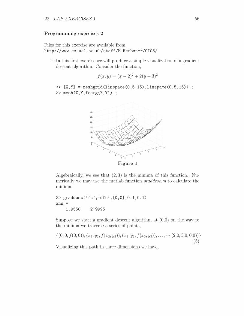
1. In this first exercise we will produce a simple visualization of a gradientdescent algorithm. Consider the function,
f(x, y) = (x − 2)2 + 2(y − 3)2
>> [X,Y] = meshgrid(linspace(0,5,15),linspace(0,5,15)) ;
>> mesh(X,Y,fcarg(X,Y)) ;
01
23
45
0
1
2
3
4
50
5
10
15
20
25
30
Figure 1
Algebraically, we see that (2, 3) is the minima of this function. Nu-merically we may use the matlab function graddesc.m to calculate theminima.
>> graddesc(’fc’,’dfc’,[0,0],0.1,0.1)
ans =
1.9550 2.9995
Suppose we start a gradient descent algorithm at (0,0) on the way tothe minima we traverse a series of points,
{(0, 0, f(0, 0)), (x2, y2, f(x2, y2)), (x3, y3, f(x3, y3)), . . . ,∼ (2.0, 3.0, 0.0))}(5)
Visualizing this path in three dimensions we have,

22 LAB EXERCISES 1 57
0
0.5
1
1.5
2
00.5
11.5
22.5
30
5
10
15
20
25
Figure 2
Projecting down to the xy plane we have,
0 0.2 0.4 0.6 0.8 1 1.2 1.4 1.6 1.8 20
0.5
1
1.5
2
2.5
3
Figure 3
(a) Produce a plot similar to Figure 1.
(b) Modify the function graddesc.m to produce a sequence of pointsas in Equation 1.
i. Modify the code.
ii. Produce a plot similar to Figure 2. (Hint: to do this it willbe necessary to massage the sequence of points into a formusable by plot3(), then to produce the grid use the commandgrid on.
iii. Produce a plot similar to Figure 3.
22 LAB EXERCISES 1 58
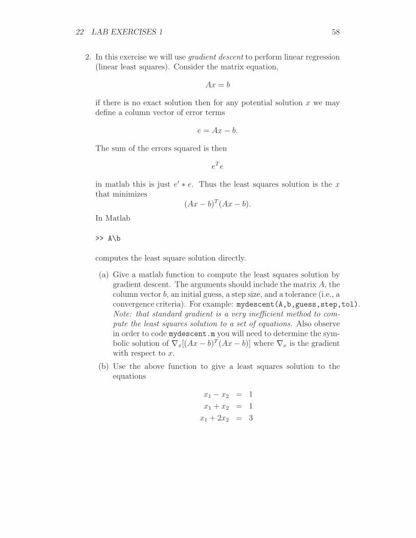
2. In this exercise we will use gradient descent to perform linear regression(linear least squares). Consider the matrix equation,
Ax = b
if there is no exact solution then for any potential solution x we maydefine a column vector of error terms
e = Ax − b.
The sum of the errors squared is then
eT e
in matlab this is just e′ ∗ e. Thus the least squares solution is the x
that minimizes(Ax − b)T (Ax − b).
In Matlab
>> A\b
computes the least square solution directly.
(a) Give a matlab function to compute the least squares solution bygradient descent. The arguments should include the matrix A, thecolumn vector b, an initial guess, a step size, and a tolerance (i.e., aconvergence criteria). For example: mydescent(A,b,guess,step,tol).Note: that standard gradient is a very inefficient method to com-pute the least squares solution to a set of equations. Also observein order to code mydescent.m you will need to determine the sym-bolic solution of ∇x[(Ax − b)T (Ax − b)] where ∇x is the gradientwith respect to x.
(b) Use the above function to give a least squares solution to theequations
x1 − x2 = 1
x1 + x2 = 1
x1 + 2x2 = 3
22 LAB EXERCISES 1 59
(c) Visualize the above solution with a plot as in Figure 3.
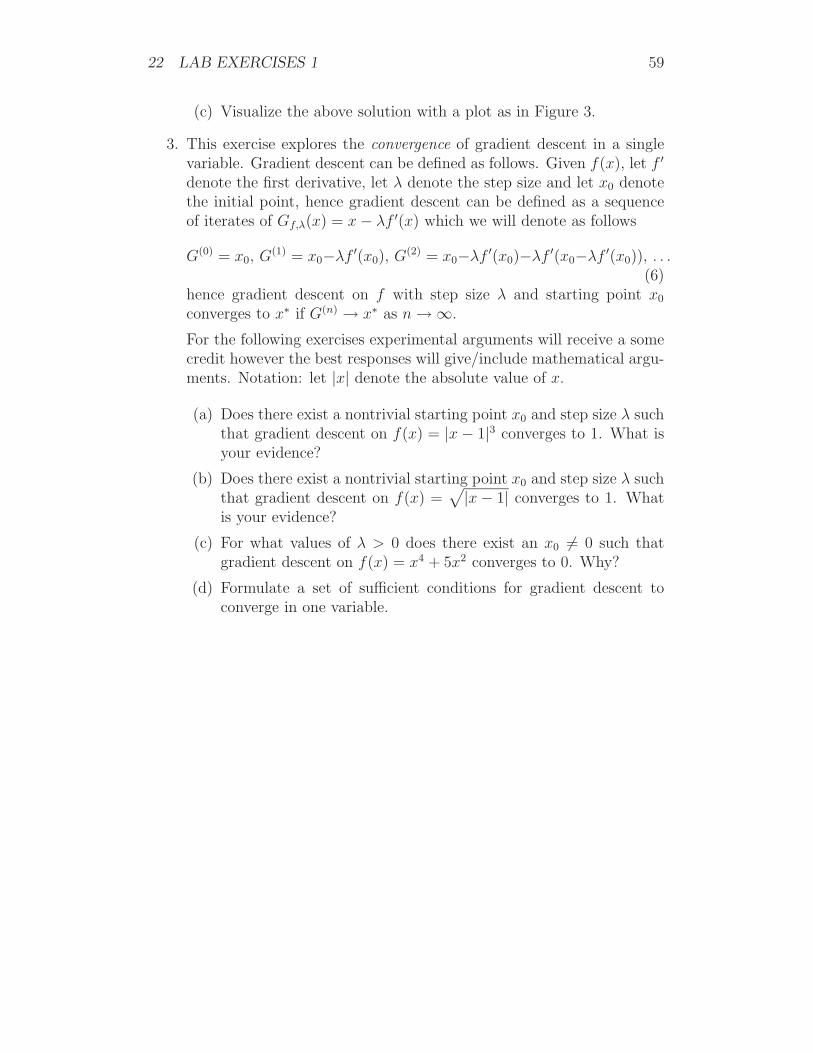
3. This exercise explores the convergence of gradient descent in a singlevariable. Gradient descent can be defined as follows. Given f(x), let f ′
denote the first derivative, let λ denote the step size and let x0 denotethe initial point, hence gradient descent can be defined as a sequenceof iterates of Gf,λ(x) = x − λf ′(x) which we will denote as follows
G(0) = x0, G(1) = x0−λf ′(x0), G(2) = x0−λf ′(x0)−λf ′(x0−λf ′(x0)), . . .
(6)hence gradient descent on f with step size λ and starting point x0
converges to x∗ if G(n) → x∗ as n → ∞.
For the following exercises experimental arguments will receive a somecredit however the best responses will give/include mathematical argu-ments. Notation: let |x| denote the absolute value of x.
(a) Does there exist a nontrivial starting point x0 and step size λ suchthat gradient descent on f(x) = |x − 1|3 converges to 1. What isyour evidence?
(b) Does there exist a nontrivial starting point x0 and step size λ suchthat gradient descent on f(x) =
√
|x − 1| converges to 1. Whatis your evidence?
(c) For what values of λ > 0 does there exist an x0 6= 0 such thatgradient descent on f(x) = x4 + 5x2 converges to 0. Why?
(d) Formulate a set of sufficient conditions for gradient descent toconverge in one variable.
60
Part III
Lecture 2
23 Overview of Lecture 2
• Relational operators
• Logical operators
• Control flow
for loops
while loops
if-else-end
switch-case-otherwise-end
• Precision issues
• Additional data types
Strings
Cell arrays
Structures
• Input/Output (I/O)
• Formatted Input/Output
• Summary table of functions
24 RELATIONAL OPERATORS 61
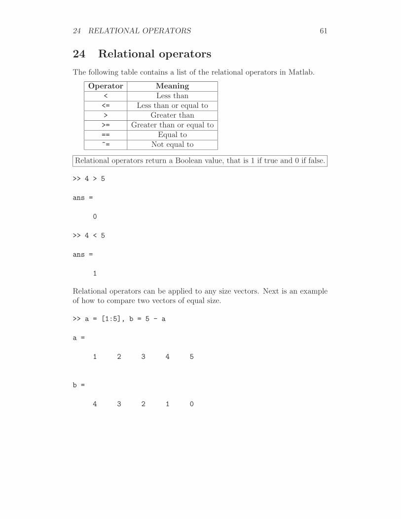
24 Relational operators
The following table contains a list of the relational operators in Matlab.
Operator Meaning< Less than<= Less than or equal to> Greater than>= Greater than or equal to== Equal to~= Not equal to
Relational operators return a Boolean value, that is 1 if true and 0 if false.
>> 4 > 5
ans =
0
>> 4 < 5
ans =
1
Relational operators can be applied to any size vectors. Next is an exampleof how to compare two vectors of equal size.
>> a = [1:5], b = 5 - a
a =
1 2 3 4 5
b =
4 3 2 1 0
24 RELATIONAL OPERATORS 62
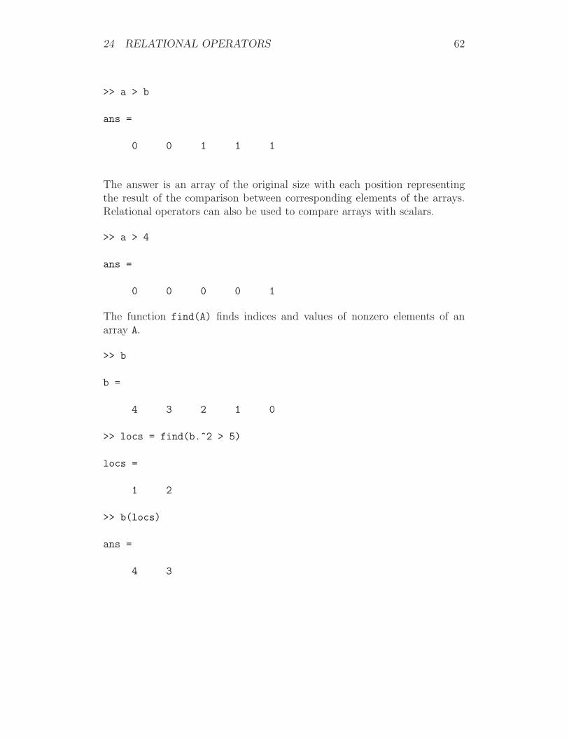
>> a > b
ans =
0 0 1 1 1
The answer is an array of the original size with each position representingthe result of the comparison between corresponding elements of the arrays.Relational operators can also be used to compare arrays with scalars.
>> a > 4
ans =
0 0 0 0 1
The function find(A) finds indices and values of nonzero elements of anarray A.
>> b
b =
4 3 2 1 0
>> locs = find(b.^2 > 5)
locs =
1 2
>> b(locs)
ans =
4 3

25 LOGICAL OPERATORS 63
25 Logical operators
The following table lists the logical operators in Matlab. Note that A and B
are not considered purely as matrices but as logical expressions.
Operator Function Form Meaning& and(A,B) and| or(A,B) inclusive or
xor(A,B) exclusive or~ not(A) not
The operator and (&) requires both expressions A, B to be true in orderto return true, all other combinations return false. The inclusive or (|)returns true if one or both of the expressions are true, while the exclusiveor (xor(A,B)) returns true only if one expression is true and returns false ifboth expressions are true or false. The operator not (~) returns true if theexpression is false and false if the expression is true. This can be summarizedin a truth table.
A B A&B A|B xor(A,B) ~A
0 0 0 0 0 11 0 0 1 1 00 1 0 1 1 11 1 1 1 0 0
These operators are used in the following way. Consider A and B to be twological expressions with a Boolean value, that is 1 for true and 0 for false.
>> A = 0; B = 1;
>> A & B
ans =
0
>> A | B
ans =
1
25 LOGICAL OPERATORS 64
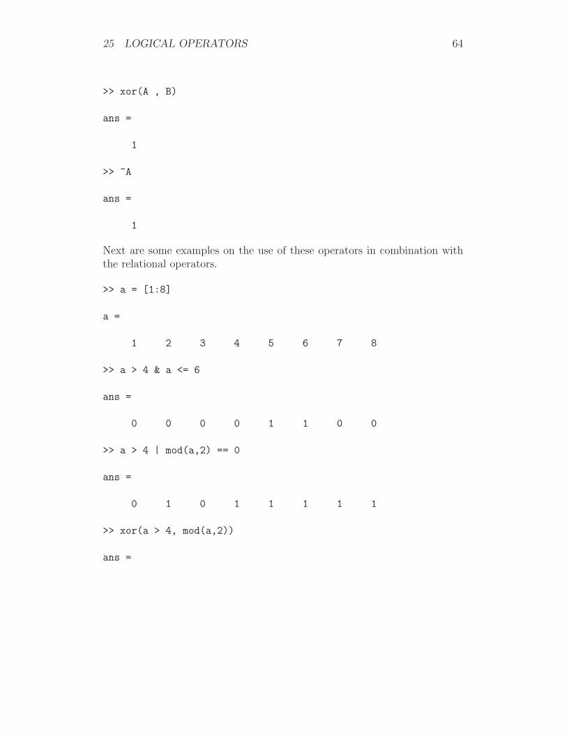
>> xor(A , B)
ans =
1
>> ~A
ans =
1
Next are some examples on the use of these operators in combination withthe relational operators.
>> a = [1:8]
a =
1 2 3 4 5 6 7 8
>> a > 4 & a <= 6
ans =
0 0 0 0 1 1 0 0
>> a > 4 | mod(a,2) == 0
ans =
0 1 0 1 1 1 1 1
>> xor(a > 4, mod(a,2))
ans =

26 CONTROL FLOW 65
1 0 1 0 0 1 0 1
>> a > 4 & (~mod(a,2) == 0 )
ans =
0 0 0 0 1 0 1 0
The mod(a,b) function calculates the modulus after the division a/b. Thenot operator can usually be replaced by directly negating the expression.The last expression on the previous example can be rewritten as:
>> a > 4 & (mod(a,2) ~= 0 )
ans =
0 0 0 0 1 0 1 0
It is also possible to build expressions combining multiple logical operators.
>> (a > 4 & a <= 6) | (a == 1)
ans =
1 0 0 0 1 1 0 0
26 Control flow
In the following sections the control flow of loops (for, while - end) andconditional statements (if - else, switch - case) will be introduced.
26.1 for loops
The most common way of repeating a sequence of statements for a specificnumber of times is to use a for loop. Consider the following example:
26 CONTROL FLOW 66
>> for x=1:2
disp(’This statement is repeated’)
end
The statement between for and end will be repeated two times. The outputon the screen will be:
This statement is repeated
This statement is repeated
On the first line of the loop, starting with for, we define how many timesthe statements will be repeated. If we simply change the 2 from the previousexample to 3, the statements will be repeated three times.
>> for x=1:3
disp(’This statement is repeated’)
end
The function disp(a) displays a on to the screen. The output on the screenwill be:
This statement is repeated
This statement is repeated
This statement is repeated
The first line of the loop contains an assignment of an array. The numberof columns of this array defines how many times the statements inside theloop will be executed. On every repetition x will be equal to a column ofthe array it was assigned to. The variable x will take consecutive values, thecolumns, of the assigned array. Consider the following example:
>> for x = [1 3 5]
disp(’x equals’),disp(x)
end
The output on the screen will be:
26 CONTROL FLOW 67
x equals
1
x equals
3
x equals
5
The statement disp(’x equals’),disp(x) was repeated three times, thatis the number of columns of the array [1 3 5] used in the assignment, eachtime taking the value of the column of the array [1 3 5]. A matrix can alsobe used instead of vector. In this case x will be a column vector instead of asingle number.
>> for x = [1 2 3; 4 5 6]
disp(’x equals’),disp(x)
end
The output on the screen will be:
x equals
1
4
x equals
2
5
x equals
3
6
The general syntax of the for loop is as follows:
26 CONTROL FLOW 68
for x=array
statements % executed once for each column in array
% x is the columns consecutively
end
The first line defines how many times statements will be executed. If arrayis a m × n matrix then statements will be executed n times. Each time x
will be equal to the corresponding column.The following example calculates and displays the mean and the sum of
each column of a matrix.
>> A=[1:12]; B = reshape(A,4,3)
B =
1 5 9
2 6 10
3 7 11
4 8 12
>> for x=B
disp(’Mean:’); disp(mean(x)); disp(’Sum:’); disp(sum(x));
end
Mean:
2.5000
Sum:
10
Mean:
6.5000
Sum:
26
Mean:
10.5000
26 CONTROL FLOW 69
Sum:
42
The function reshape(A,r,c) reshapes A in to r rows and c columns. Thefunctions mean(a) and sum(a) calculated the mean and sum of a. If a is amatrix then they calculate the mean or sum on each column of a.
In the case where x takes consecutive integer values it can be used as anindex in array.
>> a = [1,2,3];
>> for x=a
b(x) = x^2;
end
>> b
b =
1 4 9
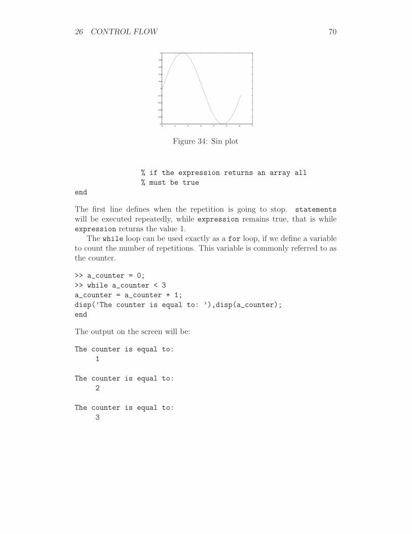
>> x_values = [0:0.1:2*pi - 0.1];
>> for index=1:length(x_values)
y_values(index) = sin(x_values(index));
end
>> figure;plot(x_values,y_values);
Question: How can we simplify the above example and avoid using a for
loop?The function length(a) returns the size of the largest dimension of a.
The last statement will produce the plot in fig. 34.
26.2 while loops
Often we wish to repeat a sequence of statements while a given conditionremains true. The general syntax for a while loop is the following.
while expression
statements % are executed while expression is true
26 CONTROL FLOW 70
0 1 2 3 4 5 6 7−1
−0.8
−0.6
−0.4
−0.2
0
0.2
0.4
0.6
0.8
1
Figure 34: Sin plot
% if the expression returns an array all
% must be true
end
The first line defines when the repetition is going to stop. statements
will be executed repeatedly, while expression remains true, that is whileexpression returns the value 1.
The while loop can be used exactly as a for loop, if we define a variableto count the number of repetitions. This variable is commonly referred to asthe counter.
>> a_counter = 0;
>> while a_counter < 3
a_counter = a_counter + 1;
disp(’The counter is equal to: ’),disp(a_counter);
end
The output on the screen will be:
The counter is equal to:
1
The counter is equal to:
2
The counter is equal to:
3

26 CONTROL FLOW 71
Next is an example that finds the first non zero entry of an array or amatrix and stores its index.
>> A = zeros(10,1);
>> A(5) = 1;
>> m = 1;
>> while A(m) == 0
m = m + 1;
end
>> m
m =
5
Question: How can the above example be accomplished using the functionfind()?
The difference between the two types of loops is that for loops can onlyrepeat statements based on the number of columns of the assigned array.while loops can repeat statements based on any expression. Thus whileloops are more general than for loops. The most common use of for loopsis for counting type of repetitions, their advantage there is that they havethe counter build in to the syntax.
26.3 if-else-end
To execute different sequences of statements according to some conditionswe can use if-else-end. The general syntax is as follows:
if expression1
statements1 % executed if expression1 is true
elseif expression2
statements2 % executed if expression1 is false and expression2 is true
elseif expression3
statements3 % executed if all previous expressions are false
.... % and expression3 is true
else
statements4 % executed if no expression is true
end

26 CONTROL FLOW 72
Note that expression2 will only be checked if expression1 is false.
The next expression will only be checked if the previous one is false. Thatmeans that if two or more expressions are true, only the first one is goingto be executed.
To demonstrate this a simple example of if-else follows next.
>>if 1<2
disp(’First condition’);
elseif 1<3
disp(’Second condition’);
end
First if-else
The following function uses if-else to separate an array of numbers intonumbers divisible by 2, divisible by 3 and not divisible by 2 or 3.
function [div_2, div_3, not_div] = myseparate(A)
% rtn = mysort(A) takes a scalar vector as input
% and sorts it out to numbers that are divisible by 2 (div_2),
% numbers that are divisible by 3 (div_3) and
% other numbers that are not divisible by 2 or 3.
% If a number is divisible by 2 and 3 then it will go to both lists.
count_div_2 = 0; count_div_3 = 0; count_not_div = 0;
for m=1:length(A)
if mod(A(m),2) == 0 & mod(A(m),3) == 0
count_div_2 = count_div_2 + 1;
div_2(count_div_2) = A(m);
count_div_3 = count_div_3 + 1;
div_3(count_div_3) = A(m);
elseif mod(A(m),2) == 0
count_div_2 = count_div_2 + 1;
div_2(count_div_2) = A(m);
elseif mod(A(m),3) == 0
count_div_3 = count_div_3 + 1;
26 CONTROL FLOW 73
div_3(count_div_3) = A(m);
else
count_not_div = count_not_div + 1;
not_div(count_not_div) = A(m);
end
end
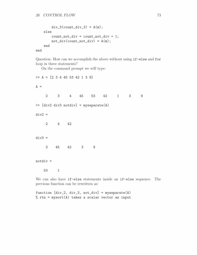
Question: How can we accomplish the above without using if-else and for
loop in three statements?On the command prompt we will type:
>> A = [2 3 4 45 53 42 1 3 9]
A =
2 3 4 45 53 42 1 3 9
>> [div2 div3 notdiv] = myseparate(A)
div2 =
2 4 42
div3 =
3 45 42 3 9
notdiv =
53 1
We can also have if-else statements inside an if-else sequence. Theprevious function can be rewritten as:
function [div_2, div_3, not_div] = myseparate(A)
% rtn = mysort(A) takes a scalar vector as input

26 CONTROL FLOW 74
% and sorts it out to numbers that are divisible by 2 (div_2),
% numbers that are divisible by 3 (div_3) and
% other numbers that are not divisible by 2 or 3.
% If a number is divisible by 2 and 3 then it will go to both lists.
count_div_2 = 0; count_div_3 = 0; count_not_div = 0;
for m=1:length(A)
if mod(A(m),2) == 0
count_div_2 = count_div_2 + 1;
div_2(count_div_2) = A(m);
if mod(A(m),3) == 0
count_div_3 = count_div_3 + 1;
div_3(count_div_3) = A(m);
end
elseif mod(A(m),3) == 0
count_div_3 = count_div_3 + 1;
div_3(count_div_3) = A(m);
else
count_not_div = count_not_div + 1;
not_div(count_not_div) = A(m);
end
end
26.4 switch-case-otherwise-end
Another method of executing statements according to some conditions is touse switch-case-otherwise-end.
switch expression
case result1
statements1 % executed if the result from expression
% is equal to result1
case result2
statements2 % executed if the result from expression is not equal
% to result1 and it is equal to result2
case result3

26 CONTROL FLOW 75
statements3 % executed if the result from expression is not equal to
% any of the previous results and is equal to result3
...
otherwise
statements4 % executed if the result from expression is
% not equal to any of the previous results
end
Similarly to if-else, further statementswill only be executed if the resultsfrom the previous are not equal to the result of expression.
The following function converts the month number in to the name of themonth.
function [rtn] = disp_month (num_month)
% [rtn] = disp_month (num_month)
% takes a number as an argument (num_month), displays
% the equivalent month with each name and
% and returns 1 if the month exists and 0 otherwise
rtn = 1;
switch num_month
case 1
disp(’Month entered is January’);
case 2
disp(’Month entered is February’);
case 3
disp(’Month entered is March’);
case 4
disp(’Month entered is April’);
case 5
disp(’Month entered is May’);
case 6
disp(’Month entered is June’);
case 7
disp(’Month entered is July’);
case 8
disp(’Month entered is August’);
case 9
27 PRECISION ISSUES 76
disp(’Month entered is September’);
case 10
disp(’Month entered is October’);
case 11
disp(’Month entered is November’);
case 12
disp(’Month entered is December’);
otherwise
disp(’Month entered does not exist’);
rtn = 0;
end
On the command prompt we can type:
>> true_false = disp_month(8);
Month entered is August
>> true_false
true_false =
1
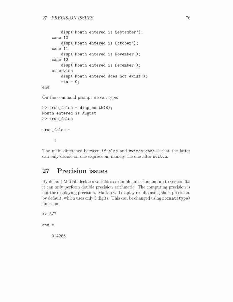
The main difference between if-else and switch-case is that the lattercan only decide on one expression, namely the one after switch.
27 Precision issues
By default Matlab declares variables as double precision and up to version 6.5it can only perform double precision arithmetic. The computing precision isnot the displaying precision. Matlab will display results using short precision,by default, which uses only 5 digits. This can be changed using format(type)function.
>> 3/7
ans =
0.4286

27 PRECISION ISSUES 77
>> format(’long’)
>> 3/7
ans =
0.42857142857143
>> format(’long’, ’e’)
>> 3/7
ans =
4.285714285714286e-001
Variables can also be defined to be of a specific type (single(A), double(A),int8, int16(A), int32(A), int64(A), uint8(A), uint16(A), ...). These areall primitive types. int8 uses 8 bits and it can take any of the 28 possiblevalues of signed integers. That means that it can take values from -128(−27)to 127(27 − 1). uint8 also uses 8 bit, but it can only take unsigned valuesfrom 0 to 255(28 − 1). int16 uses 16 bits for signed integers from −215 to215 − 1. uint16 also uses 16 bits for unsigned integers and takes values from0 to 216 − 1. The rest of the integer data types are defined in the same way.
double is the only one, which can be used for mathematical operations upto Matlab version 6.5.
In Matlab version 7 mathematical operations can be performed betweenvariables that belong to the same type, or between variables that belong todouble and variables that belong to one other type (that can be any type aslong as everything that is not double belongs to one type). Mathematicaloperations between different types, with the exception of double mentionedabove, can not be performed.
The next example is in Matlab version 7:
>> a = int16(1); b = int16(2);
>> a_b = a + b
a_b =

27 PRECISION ISSUES 78
3
>> c = double(3);
>> b_c = b + c
b_c =
5
>> d = int8(4);
>> a_d = a + d
??? Error using ==> plus Integers can only be combined with
integers of the same class, or scalar doubles.
>> whos
Name Size Bytes Class
a 1x1 2 int16 array
a_b 1x1 2 int16 array
b 1x1 2 int16 array
b_c 1x1 2 int16 array
c 1x1 8 double array
d 1x1 1 int8 array
Grand total is 6 elements using 17 bytes
In Matlab version 6.5 we would get:
>> a = int16(1); b = int16(2);
>> a_b = a + b
??? Error using ==> + Function ’+’ is not defined for values of
class ’int16’.
>> c = double(3);
>> b_c = b + c
??? Error using ==> + Function ’+’ is not defined for values of
class ’int16’.

27 PRECISION ISSUES 79
This error can appear when reading in data from a file, like an image andthen trying to perform a mathematical operation. The solution is simply toconvert them to double.
>> a = double(a), b = double(b)
a =
2
b =
3
>> a + b
ans =
5
Matlab can be inexact sometimes. Consider the following example:
>> (-0.08 + 0.5 - 0.42) == (0.5 - 0.42 - 0.08)
ans =
0
>> (-0.08 + 0.5 - 0.42) ~= (0.5 - 0.42 - 0.08)
ans =
1
>> (-0.08 + 0.5 - 0.42) - (0.5 - 0.42 - 0.08)
ans =
27 PRECISION ISSUES 80
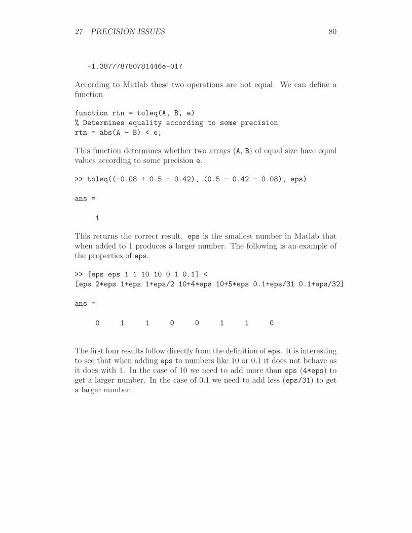
-1.387778780781446e-017
According to Matlab these two operations are not equal. We can define afunction
function rtn = toleq(A, B, e)
% Determines equality according to some precision
rtn = abs(A - B) < e;
This function determines whether two arrays (A, B) of equal size have equalvalues according to some precision e.
>> toleq((-0.08 + 0.5 - 0.42), (0.5 - 0.42 - 0.08), eps)
ans =
1
This returns the correct result. eps is the smallest number in Matlab thatwhen added to 1 produces a larger number. The following is an example ofthe properties of eps.
>> [eps eps 1 1 10 10 0.1 0.1] <
[eps 2*eps 1+eps 1+eps/2 10+4*eps 10+5*eps 0.1+eps/31 0.1+eps/32]
ans =
0 1 1 0 0 1 1 0
The first four results follow directly from the definition of eps. It is interestingto see that when adding eps to numbers like 10 or 0.1 it does not behave asit does with 1. In the case of 10 we need to add more than eps (4*eps) toget a larger number. In the case of 0.1 we need to add less (eps/31) to geta larger number.
28 ADDITIONAL DATA TYPES 81
28 Additional data types
So far we have used mainly arrays that hold scalar values. In Matlab wecan also define strings (arrays of characters), cell arrays and structures. Cellarrays and structures are composite types.
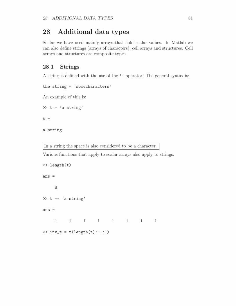
28.1 Strings
A string is defined with the use of the ’’ operator. The general syntax is:
the_string = ’somecharacters’
An example of this is:
>> t = ’a string’
t =
a string
In a string the space is also considered to be a character.
Various functions that apply to scalar arrays also apply to strings.
>> length(t)
ans =
8
>> t == ’a string’
ans =
1 1 1 1 1 1 1 1
>> inv_t = t(length(t):-1:1)
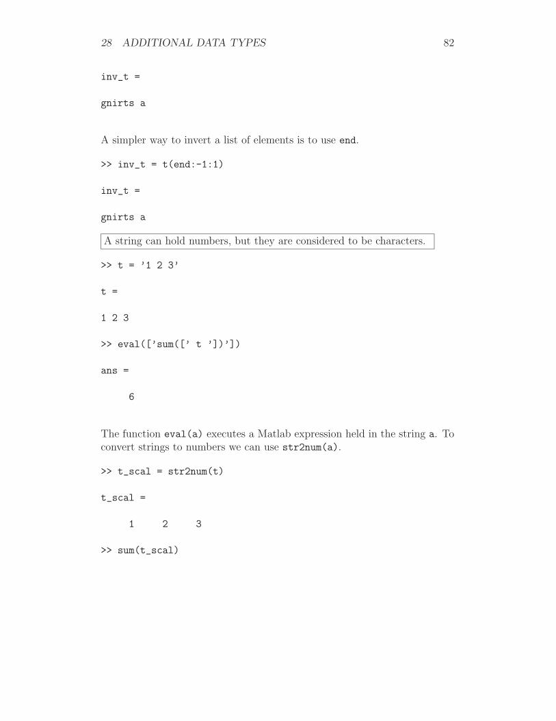
28 ADDITIONAL DATA TYPES 82
inv_t =
gnirts a
A simpler way to invert a list of elements is to use end.
>> inv_t = t(end:-1:1)
inv_t =
gnirts a
A string can hold numbers, but they are considered to be characters.
>> t = ’1 2 3’
t =
1 2 3
>> eval([’sum([’ t ’])’])
ans =
6
The function eval(a) executes a Matlab expression held in the string a. Toconvert strings to numbers we can use str2num(a).
>> t_scal = str2num(t)
t_scal =
1 2 3
>> sum(t_scal)

28 ADDITIONAL DATA TYPES 83
ans =
6
It is also possible to convert numbers to strings using num2str(a).
>> t_scal = [1 2 3]
t_scal =
1 2 3
>> t = num2str(t_scal)
t =
1 2 3
28.2 Cell arrays
Cell arrays can hold multiple data types. It is possible for example to have astring, various types of matrices as well as a cell array inside a cell array. Cellarrays are constructed with the use of the curly brackets {}, this is analogousto the square bracket [] constructor of arrays.
>> A = {[1 2 3 ; 4 5 6] ’hello world’ ; 4 {’red’ [10 11 12]}}
A =
[2x3 double] ’hello world’
[ 4] {1x2 cell}
>> celldisp(A)
A{1,1} =
1 2 3
28 ADDITIONAL DATA TYPES 84
4 5 6
A{2,1} =
4
A{1,2} =
hello world
A{2,2}{1} =
red
A{2,2}{2} =
10 11 12
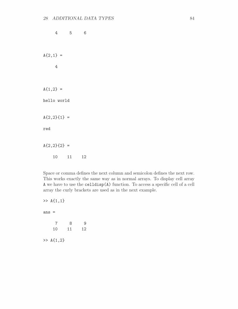
Space or comma defines the next column and semicolon defines the next row.This works exactly the same way as in normal arrays. To display cell arrayA we have to use the celldisp(A) function. To access a specific cell of a cellarray the curly brackets are used as in the next example.
>> A{1,1}
ans =
7 8 9
10 11 12
>> A{1,2}

28 ADDITIONAL DATA TYPES 85
ans =
hello world
>> A{2,2}
ans =
’red’ [1x3 double]
To access a specific element of any data type inside a cell, we will use theequivalent operator immediately after the curly brackets. If it is an array ora string we will use round brackets (), if it is another cell we will use curlybrackets {}.
>> A{1,1}
ans =
1 2 3
4 5 6
>> A{1,1}(2,2)
ans =
5
>> A{2,2}
ans =
’red’ [1x3 double]
>> A{2,2}{2}([1 3])
ans =

28 ADDITIONAL DATA TYPES 86
10 12
It is also possible to construct arrays of cell arrays and cell arrays of cellarrays.
>> {A ; A}
ans =
{2x2 cell}
{2x2 cell}
>> [A ; A]
ans =
[2x3 double] ’hello world’
[ 4] {1x2 cell}
[2x3 double] ’hello world’
[ 4] {1x2 cell}
28.3 Structures
Another method of having multiple data types within a single variable is touse structures. Structures have a field and each field can hold any data type.A field is defined after the full stop(.) .
>> data.the_values = [1 2 3; 4 5 6; 7 8 9];
>> data.the_max = max(max(data.the_values));
>> data.the_min = min(min(data.the_values));
>> data.the_mean = mean(mean(data.the_values));
>> data
data =
the_values: [3x3 double]
28 ADDITIONAL DATA TYPES 87
the_max: 9
the_min: 1
the_mean: 5
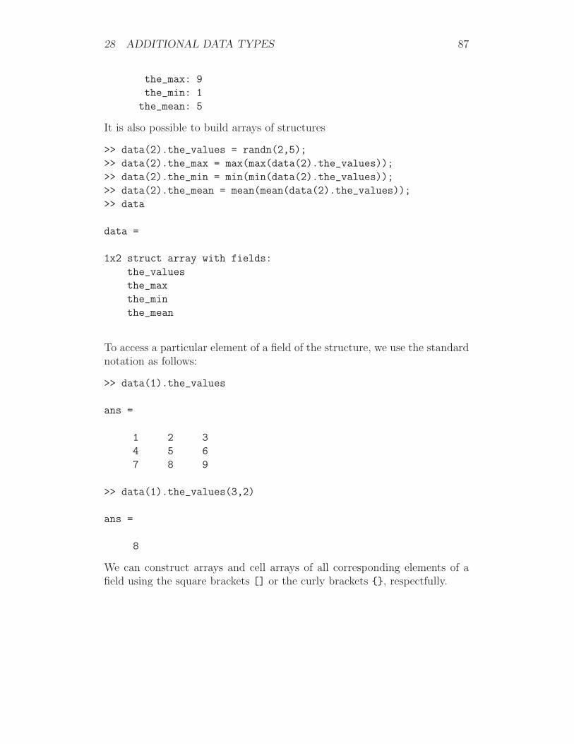
It is also possible to build arrays of structures
>> data(2).the_values = randn(2,5);
>> data(2).the_max = max(max(data(2).the_values));
>> data(2).the_min = min(min(data(2).the_values));
>> data(2).the_mean = mean(mean(data(2).the_values));
>> data
data =
1x2 struct array with fields:
the_values
the_max
the_min
the_mean
To access a particular element of a field of the structure, we use the standardnotation as follows:
>> data(1).the_values
ans =
1 2 3
4 5 6
7 8 9
>> data(1).the_values(3,2)
ans =
8
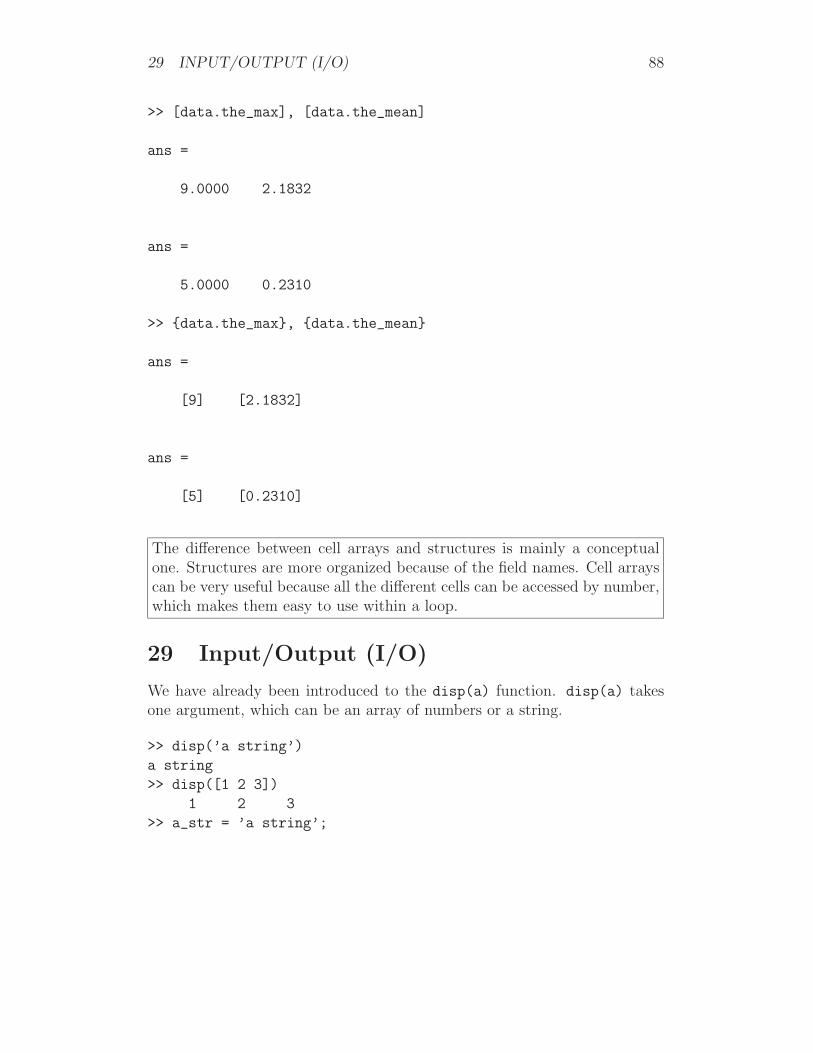
We can construct arrays and cell arrays of all corresponding elements of afield using the square brackets [] or the curly brackets {}, respectfully.
29 INPUT/OUTPUT (I/O) 88
>> [data.the_max], [data.the_mean]
ans =
9.0000 2.1832
ans =
5.0000 0.2310
>> {data.the_max}, {data.the_mean}
ans =
[9] [2.1832]
ans =
[5] [0.2310]
The difference between cell arrays and structures is mainly a conceptualone. Structures are more organized because of the field names. Cell arrayscan be very useful because all the different cells can be accessed by number,which makes them easy to use within a loop.
29 Input/Output (I/O)
We have already been introduced to the disp(a) function. disp(a) takesone argument, which can be an array of numbers or a string.
>> disp(’a string’)
a string
>> disp([1 2 3])
1 2 3
>> a_str = ’a string’;
30 FORMATTED INPUT/OUTPUT 89
>> disp(a_str)
a string
>> a = [1 2 3];
>> disp(a)
1 2 3
>> disp([a_str, ’and ’ , num2str(a)])
a stringand 1 2 3
In the last example we have combined two strings and a numerical variable,which was converted into a string using num2str. To obtain an input fromthe user, we can use the input(a), where a is string. The user can inputany kind of data.
>> A = [1 2 3];
>> B = input(’Enter a matrix: ’);
Enter a matrix: [100:100:300]
>> A + B
ans =
101 202 303
>> B = input(’Enter a matrix: ’);
Enter a matrix: A
>> A + B
ans =
2 4 6
30 Formatted Input/Output
For formatted input/output and general file handling we have fopen, fclose,fread, fwrite, fprintf, fscanf, sprintf, sscanf, ferror, feof and fseak.All these functions are equivalent to the programming language ANSI C.These functions will prove very useful when reading data from a file or writ-ing data to a file.

30 FORMATTED INPUT/OUTPUT 90
Function Meaningfopen(’filename’,’flag’) Open a file
fclose(fid) Close a filefread(fid) Read binary data from a file
fwrite(fid,A,’precision’) Write binary data A to a filefprintf(fid,format,A) Write formatted data to a filefscanf(fid,format,A) Read formatted data from a filesprintf(format,A) Write formatted data A to a stringsscanf(s,format,A) Read string s under format control
ferror(fid) Query about file I/O errorsfeof(fid) Test for end of file
fseek(fid,offset,origin) Set the file position indicator
The functions fopen(’filename’,’flag’) and fclose(fid) open andclose a file. To be able to read data from a file, a file identifier (fid) is required.fid is returned from fid=fopen(’filename’). Note that ’filename’ is astring. The second argument of fopen(’filename’,’flag’) is a flag de-termining how we are going to process the file we have opened (read only,write,...). A file should be closed as soon as we are done reading or manipu-lating data from this file. To close the file we will use fclose(fid).
The function fwrite(fid,A,’precision’) can be used to write datain a file. The fid is obtained from the fopen function, A is the data tobe written and ’precision’ is a string defining the number of bits to bewritten. ’precision’ defines the type of data. In the following example wewill use ’char’ to write characters on to a file. For more alternatives for the’precision’ string look in Matlab’s help.
>> a = [1 2 3 8 4 5];
>> fid = fopen(’some_data_1.txt’,’w’);
>> fwrite(fid,num2str(a),’char’);
>> fclose(fid);
In the call of the fopen function the flag ’w’ was used. This defines thatthe file will be opened, or created if it does not exist, for reading and writingdiscarding any data stored in that file. We have converted the numericalvariable a to a string using num2str, in order to be compatible with the’char’ type. The previous example created a file with the following contents:
1 2 3 8 4 5
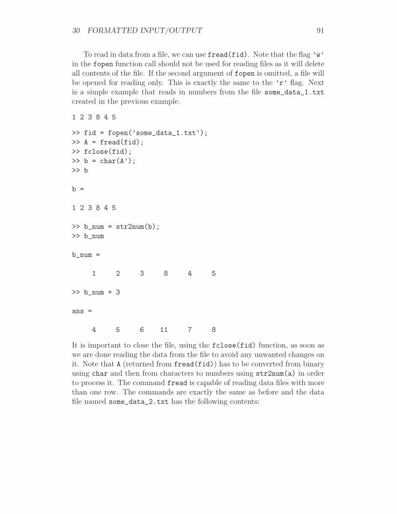
30 FORMATTED INPUT/OUTPUT 91
To read in data from a file, we can use fread(fid). Note that the flag ’w’in the fopen function call should not be used for reading files as it will deleteall contents of the file. If the second argument of fopen is omitted, a file willbe opened for reading only. This is exactly the same to the ’r’ flag. Nextis a simple example that reads in numbers from the file some_data_1.txt
created in the previous example.
1 2 3 8 4 5
>> fid = fopen(’some_data_1.txt’);
>> A = fread(fid);
>> fclose(fid);
>> b = char(A’);
>> b
b =
1 2 3 8 4 5
>> b_num = str2num(b);
>> b_num
b_num =
1 2 3 8 4 5
>> b_num + 3
ans =
4 5 6 11 7 8
It is important to close the file, using the fclose(fid) function, as soon aswe are done reading the data from the file to avoid any unwanted changes onit. Note that A (returned from fread(fid)) has to be converted from binaryusing char and then from characters to numbers using str2num(a) in orderto process it. The command fread is capable of reading data files with morethan one row. The commands are exactly the same as before and the datafile named some_data_2.txt has the following contents:
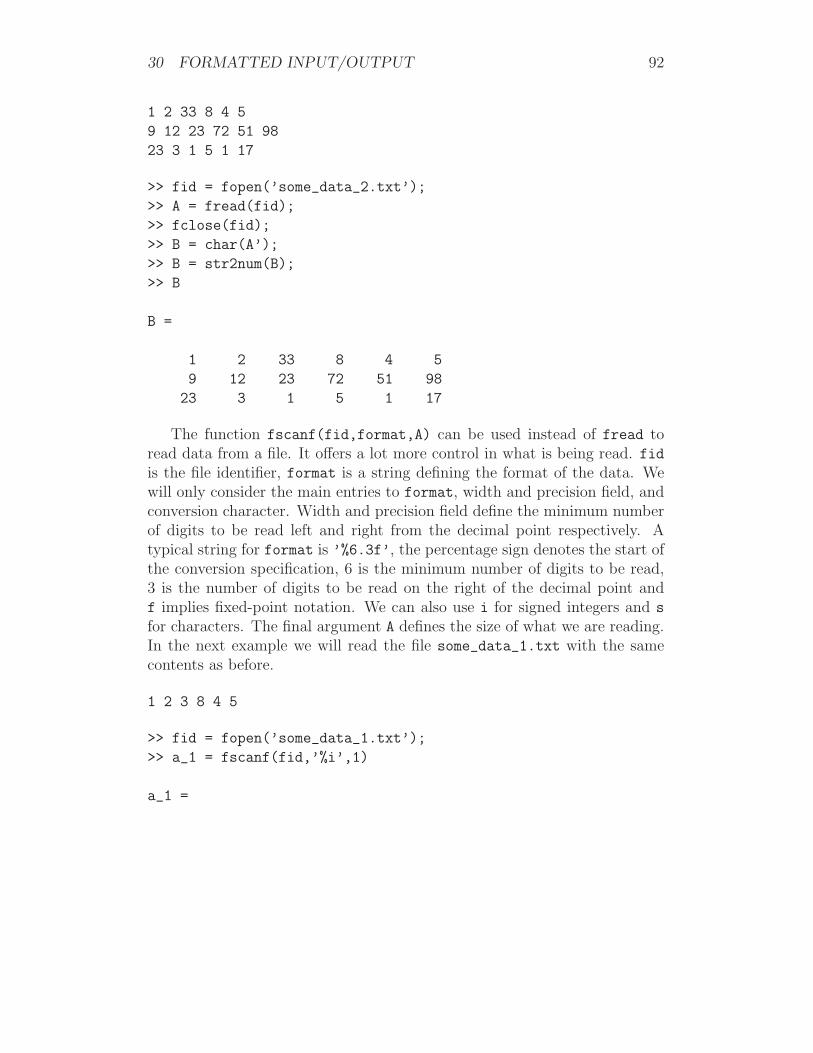
30 FORMATTED INPUT/OUTPUT 92
1 2 33 8 4 5
9 12 23 72 51 98
23 3 1 5 1 17
>> fid = fopen(’some_data_2.txt’);
>> A = fread(fid);
>> fclose(fid);
>> B = char(A’);
>> B = str2num(B);
>> B
B =
1 2 33 8 4 5
9 12 23 72 51 98
23 3 1 5 1 17
The function fscanf(fid,format,A) can be used instead of fread toread data from a file. It offers a lot more control in what is being read. fidis the file identifier, format is a string defining the format of the data. Wewill only consider the main entries to format, width and precision field, andconversion character. Width and precision field define the minimum numberof digits to be read left and right from the decimal point respectively. Atypical string for format is ’%6.3f’, the percentage sign denotes the start ofthe conversion specification, 6 is the minimum number of digits to be read,3 is the number of digits to be read on the right of the decimal point andf implies fixed-point notation. We can also use i for signed integers and s
for characters. The final argument A defines the size of what we are reading.In the next example we will read the file some_data_1.txt with the samecontents as before.
1 2 3 8 4 5
>> fid = fopen(’some_data_1.txt’);
>> a_1 = fscanf(fid,’%i’,1)
a_1 =

30 FORMATTED INPUT/OUTPUT 93
1
>> a_2 = fscanf(fid,’%i’,1)
a_2 =
2
>> a_3 = fscanf(fid,’%i’,1)
a_3 =
3
>> a_4 = fscanf(fid,’%i’,1)
a_4 =
8
>> a_5 = fscanf(fid,’%i’,1)
a_5 =
4
>> a_6 = fscanf(fid,’%i’,1)
a_6 =
5
>> fclose(fid);
Every time the fscanf function is called the file position indicator movesone position, thus the next number on the file is read. The %i conversioncharacter indicates that we are reading an integer. To simplify the code wecan put this in a loop and read the data file in to an array.
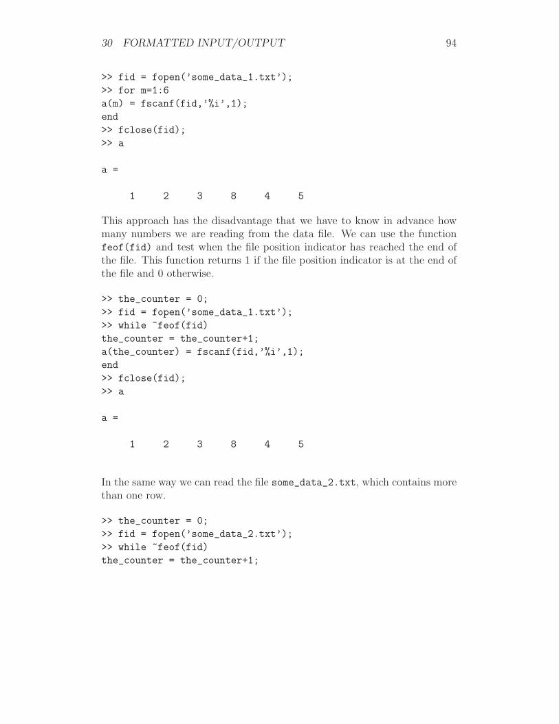
30 FORMATTED INPUT/OUTPUT 94
>> fid = fopen(’some_data_1.txt’);
>> for m=1:6
a(m) = fscanf(fid,’%i’,1);
end
>> fclose(fid);
>> a
a =
1 2 3 8 4 5
This approach has the disadvantage that we have to know in advance howmany numbers we are reading from the data file. We can use the functionfeof(fid) and test when the file position indicator has reached the end ofthe file. This function returns 1 if the file position indicator is at the end ofthe file and 0 otherwise.
>> the_counter = 0;
>> fid = fopen(’some_data_1.txt’);
>> while ~feof(fid)
the_counter = the_counter+1;
a(the_counter) = fscanf(fid,’%i’,1);
end
>> fclose(fid);
>> a
a =
1 2 3 8 4 5
In the same way we can read the file some_data_2.txt, which contains morethan one row.
>> the_counter = 0;
>> fid = fopen(’some_data_2.txt’);
>> while ~feof(fid)
the_counter = the_counter+1;

30 FORMATTED INPUT/OUTPUT 95
a(the_counter) = fscanf(fid,’%i’,1);
end
>> fclose(fid);
>> a
a =
Columns 1 through 10
1 2 33 8 4 5 9 12 23 72
Columns 11 through 18
51 98 23 3 1 5 1 17
If we wish to read the data from the file in to a matrix, we will need to knowthe number of rows in the data file.
>> fid = fopen(’some_data_2.txt’);
>> a = fscanf(fid,’%i’,[3 inf]);
>> fclose(fid);
>> a
a =
1 8 9 72 23 5
2 4 12 51 3 1
33 5 23 98 1 17
The inf in the fscanf function call stands for infinite, and it is used in orderto read as many columns as there are in file.
The next example is a function that reads data from a file containing thenames of the columns and rows and the data and loads them in to threearrays. The function is defined as follows:
function [column_name, row_name, data] = read_data(filename)
% [column_name row_name data] = read_data(filename)
% takes a string (filename) for the name

30 FORMATTED INPUT/OUTPUT 96
% and reads in the data in to three arrays. column_name is a
% string containing the names of the columns, row_name is a
% string containing the names of the rows and data is
% an array containing the data
fid = fopen(filename);
column_names_total = fscanf(fid, ’%s’,1);
start_pos = 0; end_pos = 0; count = 0;
for m=1:size(column_names_total,2)
if column_names_total(m) == ’,’
count = count + 1;
start_pos = end_pos + 1;
end_pos = m;
column_name(count,1:end_pos-start_pos)
= column_names_total(start_pos:end_pos-1);
end
end
nr_col = count;
count = 0;
while ~ feof(fid)
count = count + 1;
temp = fscanf(fid, ’%s’, 1);
row_name(count,1:length(temp)) = temp;
data(count,:) = fscanf(fid,’%g’,nr_col)’;
end
fclose(fid);
The %s and %g conversion characters are used for characters and floating-point numbers respectively. The latter is capable of reading both integer andfloating-point numbers.
Given the following data file called grades.txt:
3C71,4C65,3C24,4C54,2C44,4D98,3C70,3C65,
John 58 48 74 58 76 43 65 68

30 FORMATTED INPUT/OUTPUT 97
Bob 72 63 59 51 60 54 62 52
Jane 58 74 84 81 76 59 76 63
Mark 45 51 73 75 74 61 52 59
Lisa 47 42 51 53 48 57 64 55
Dan 55 57 75 61 68 49 51 72
Phil 59 61 63 65 72 74 73 87
Daisy 77 81 79 75 71 70 76 84
Mary 56 61 55 68 64 78 72 71
Peter 54 68 81 47 49 51 58 59
Anna 81 73 69 63 73 71 62 55
Jason 43 50 52 41 38 33 48 37
We can type on the command prompt, which will display the following:
>> [column_name, row_name, data] = read_data(’grades.txt’);
>> whos
Name Size Bytes Class
column_name 8x4 64 char array
data 12x8 768 double array
row_name 12x5 120 char array
Grand total is 188 elements using 952 bytes
The function fprintf(fid,format,A) can be used for writing data to afile or the screen. This function can take 3 arguments in the following syntaxfprintf(fid,format,A). fid and format have been introduced previously.The final argument A are the variables to be printed. In the case of readingin data (fscanf(fid,format,A), sscanf(str,format,A)) fid and format
are used in the same way. The only difference in the arguments betweenfprintf and fscanf is the third argument A. In the case of fscanf A definesthe shape of the data we are reading in, while in fprintf A is the variableto be printed.
Continuing from the previous example of reading data in from a file, wecan output maxima, minima and means of the data to the screen or a file.Next is the print_data_screen function:
function print_data_screen(column_name, row_name, data_row)
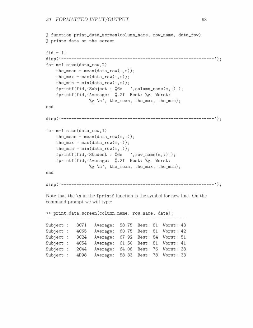
30 FORMATTED INPUT/OUTPUT 98
% function print_data_screen(column_name, row_name, data_row)
% prints data on the screen
fid = 1;
disp(’------------------------------------------------------------’);
for m=1:size(data_row,2)
the_mean = mean(data_row(:,m));
the_max = max(data_row(:,m));
the_min = min(data_row(:,m));
fprintf(fid,’Subject : %6s ’,column_name(m,:) );
fprintf(fid,’Average: %.2f Best: %g Worst:
%g \n’, the_mean, the_max, the_min);
end
disp(’------------------------------------------------------------’);
for m=1:size(data_row,1)
the_mean = mean(data_row(m,:));
the_max = max(data_row(m,:));
the_min = min(data_row(m,:));
fprintf(fid,’Student : %6s ’,row_name(m,:) );
fprintf(fid,’Average: %.2f Best: %g Worst:
%g \n’, the_mean, the_max, the_min);
end
disp(’------------------------------------------------------------’);
Note that the \n in the fprintf function is the symbol for new line. On thecommand prompt we will type:
>> print_data_screen(column_name, row_name, data);
-------------------------------------------------------
Subject : 3C71 Average: 58.75 Best: 81 Worst: 43
Subject : 4C65 Average: 60.75 Best: 81 Worst: 42
Subject : 3C24 Average: 67.92 Best: 84 Worst: 51
Subject : 4C54 Average: 61.50 Best: 81 Worst: 41
Subject : 2C44 Average: 64.08 Best: 76 Worst: 38
Subject : 4D98 Average: 58.33 Best: 78 Worst: 33
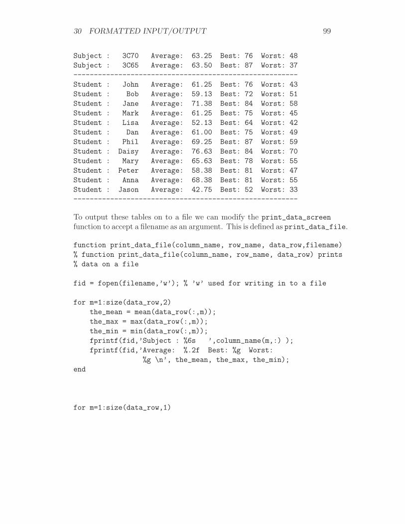
30 FORMATTED INPUT/OUTPUT 99
Subject : 3C70 Average: 63.25 Best: 76 Worst: 48
Subject : 3C65 Average: 63.50 Best: 87 Worst: 37
-------------------------------------------------------
Student : John Average: 61.25 Best: 76 Worst: 43
Student : Bob Average: 59.13 Best: 72 Worst: 51
Student : Jane Average: 71.38 Best: 84 Worst: 58
Student : Mark Average: 61.25 Best: 75 Worst: 45
Student : Lisa Average: 52.13 Best: 64 Worst: 42
Student : Dan Average: 61.00 Best: 75 Worst: 49
Student : Phil Average: 69.25 Best: 87 Worst: 59
Student : Daisy Average: 76.63 Best: 84 Worst: 70
Student : Mary Average: 65.63 Best: 78 Worst: 55
Student : Peter Average: 58.38 Best: 81 Worst: 47
Student : Anna Average: 68.38 Best: 81 Worst: 55
Student : Jason Average: 42.75 Best: 52 Worst: 33
-------------------------------------------------------
To output these tables on to a file we can modify the print_data_screen
function to accept a filename as an argument. This is defined as print_data_file.
function print_data_file(column_name, row_name, data_row,filename)
% function print_data_file(column_name, row_name, data_row) prints
% data on a file
fid = fopen(filename,’w’); % ’w’ used for writing in to a file
for m=1:size(data_row,2)
the_mean = mean(data_row(:,m));
the_max = max(data_row(:,m));
the_min = min(data_row(:,m));
fprintf(fid,’Subject : %6s ’,column_name(m,:) );
fprintf(fid,’Average: %.2f Best: %g Worst:
%g \n’, the_mean, the_max, the_min);
end
for m=1:size(data_row,1)
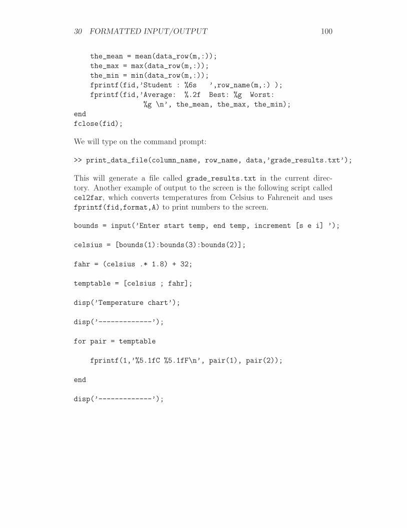
30 FORMATTED INPUT/OUTPUT 100
the_mean = mean(data_row(m,:));
the_max = max(data_row(m,:));
the_min = min(data_row(m,:));
fprintf(fid,’Student : %6s ’,row_name(m,:) );
fprintf(fid,’Average: %.2f Best: %g Worst:
%g \n’, the_mean, the_max, the_min);
end
fclose(fid);
We will type on the command prompt:
>> print_data_file(column_name, row_name, data,’grade_results.txt’);
This will generate a file called grade_results.txt in the current direc-tory. Another example of output to the screen is the following script calledcel2far, which converts temperatures from Celsius to Fahreneit and usesfprintf(fid,format,A) to print numbers to the screen.
bounds = input(’Enter start temp, end temp, increment [s e i] ’);
celsius = [bounds(1):bounds(3):bounds(2)];
fahr = (celsius .* 1.8) + 32;
temptable = [celsius ; fahr];
disp(’Temperature chart’);
disp(’-------------’);
for pair = temptable
fprintf(1,’%5.1fC %5.1fF\n’, pair(1), pair(2));
end
disp(’-------------’);
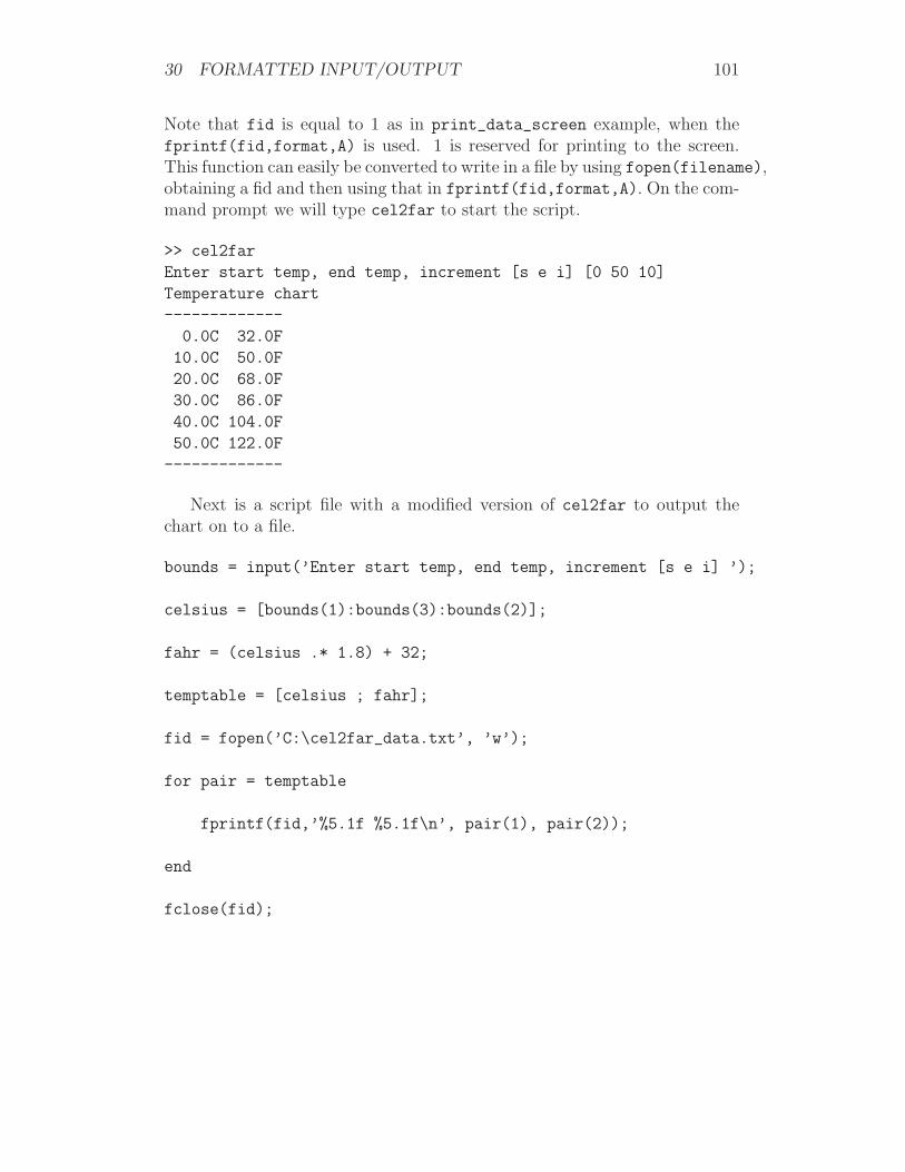
30 FORMATTED INPUT/OUTPUT 101
Note that fid is equal to 1 as in print_data_screen example, when thefprintf(fid,format,A) is used. 1 is reserved for printing to the screen.This function can easily be converted to write in a file by using fopen(filename),obtaining a fid and then using that in fprintf(fid,format,A). On the com-mand prompt we will type cel2far to start the script.
>> cel2far
Enter start temp, end temp, increment [s e i] [0 50 10]
Temperature chart
-------------
0.0C 32.0F
10.0C 50.0F
20.0C 68.0F
30.0C 86.0F
40.0C 104.0F
50.0C 122.0F
-------------
Next is a script file with a modified version of cel2far to output thechart on to a file.
bounds = input(’Enter start temp, end temp, increment [s e i] ’);
celsius = [bounds(1):bounds(3):bounds(2)];
fahr = (celsius .* 1.8) + 32;
temptable = [celsius ; fahr];
fid = fopen(’C:\cel2far_data.txt’, ’w’);
for pair = temptable
fprintf(fid,’%5.1f %5.1f\n’, pair(1), pair(2));
end
fclose(fid);

30 FORMATTED INPUT/OUTPUT 102
From the command prompt we can read the data in the following way.
>> fid = fopen(’cel2far_data.txt’);
>> A = fscanf(fid, ’%g %g’, [2 inf]);
>> A’
ans =
0 32
10 50
20 68
30 86
40 104
50 122
>> fclose(fid);
Similarly to a previous example we have used [2 inf] as the third argu-ment of fscanf(fid,format,A) for reading in the data. This will read 2 rowsand infinite number of columns. The function string = sprintf(format, A)
works exactly the same way as fprintf with the exception that it writes to astring and therefore does not require a fid. sscanf also works very similarlyto fscanf.
>> str = sprintf(’%5.0f ’,[10:17])
str =
10 11 12 13 14 15 16 17
>> A = sscanf(str, ’%f’);
>> A’
ans =
10 11 12 13 14 15 16 17
>> A = sscanf(str, ’%f’,[2 4]);

30 FORMATTED INPUT/OUTPUT 103
>> A
A =
10 12 14 16
11 13 15 17
In this example we have read data is in 2 rows and 4 columns. If we wantto save variables that are already on the workspace we can use the functionsave(’filename’,’var1’,’var2’,...). Remember that ’filename’ andthe variables are strings. If the variables var1,var2, ... are omitted, thenall variables on the workspace will be saved.
>> A = [1 2 3]; s = ’hello’; B = [1 2 ; 3 4];
>> save(’alles.mat’);
>> save(’some.mat’, ’s’, ’B’);
>> save(’B.mat’, ’B’);
>> whos -file alles.mat
Name Size Bytes Class
A 1x3 24 double array
B 2x2 32 double array
s 1x5 10 char array
Grand total is 12 elements using 66 bytes
>> whos -file some.mat
Name Size Bytes Class
B 2x2 32 double array
s 1x5 10 char array
Grand total is 9 elements using 42 bytes
>> whos -file B.mat
Name Size Bytes Class
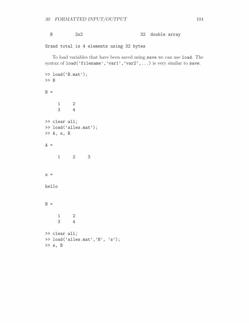
30 FORMATTED INPUT/OUTPUT 104
B 2x2 32 double array
Grand total is 4 elements using 32 bytes
To load variables that have been saved using save we can use load. Thesyntax of load(’filename’,’var1’,’var2’,...) is very similar to save.
>> load(’B.mat’);
>> B
B =
1 2
3 4
>> clear all;
>> load(’alles.mat’);
>> A, s, B
A =
1 2 3
s =
hello
B =
1 2
3 4
>> clear all;
>> load(’alles.mat’,’B’, ’s’);
>> s, B
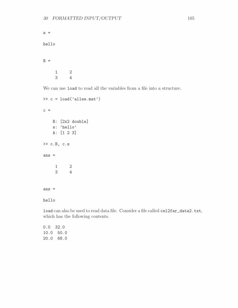
30 FORMATTED INPUT/OUTPUT 105
s =
hello
B =
1 2
3 4
We can use load to read all the variables from a file into a structure.
>> c = load(’alles.mat’)
c =
B: [2x2 double]
s: ’hello’
A: [1 2 3]
>> c.B, c.s
ans =
1 2
3 4
ans =
hello
load can also be used to read data file. Consider a file called cel2far_data2.txt,which has the following contents.
0.0 32.0
10.0 50.0
20.0 68.0
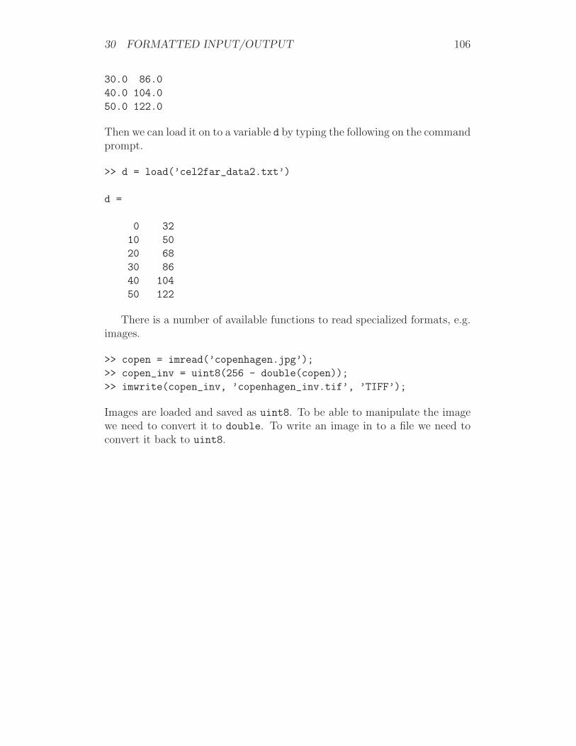
30 FORMATTED INPUT/OUTPUT 106
30.0 86.0
40.0 104.0
50.0 122.0
Then we can load it on to a variable d by typing the following on the commandprompt.
>> d = load(’cel2far_data2.txt’)
d =
0 32
10 50
20 68
30 86
40 104
50 122
There is a number of available functions to read specialized formats, e.g.images.
>> copen = imread(’copenhagen.jpg’);
>> copen_inv = uint8(256 - double(copen));
>> imwrite(copen_inv, ’copenhagen_inv.tif’, ’TIFF’);
Images are loaded and saved as uint8. To be able to manipulate the imagewe need to convert it to double. To write an image in to a file we need toconvert it back to uint8.
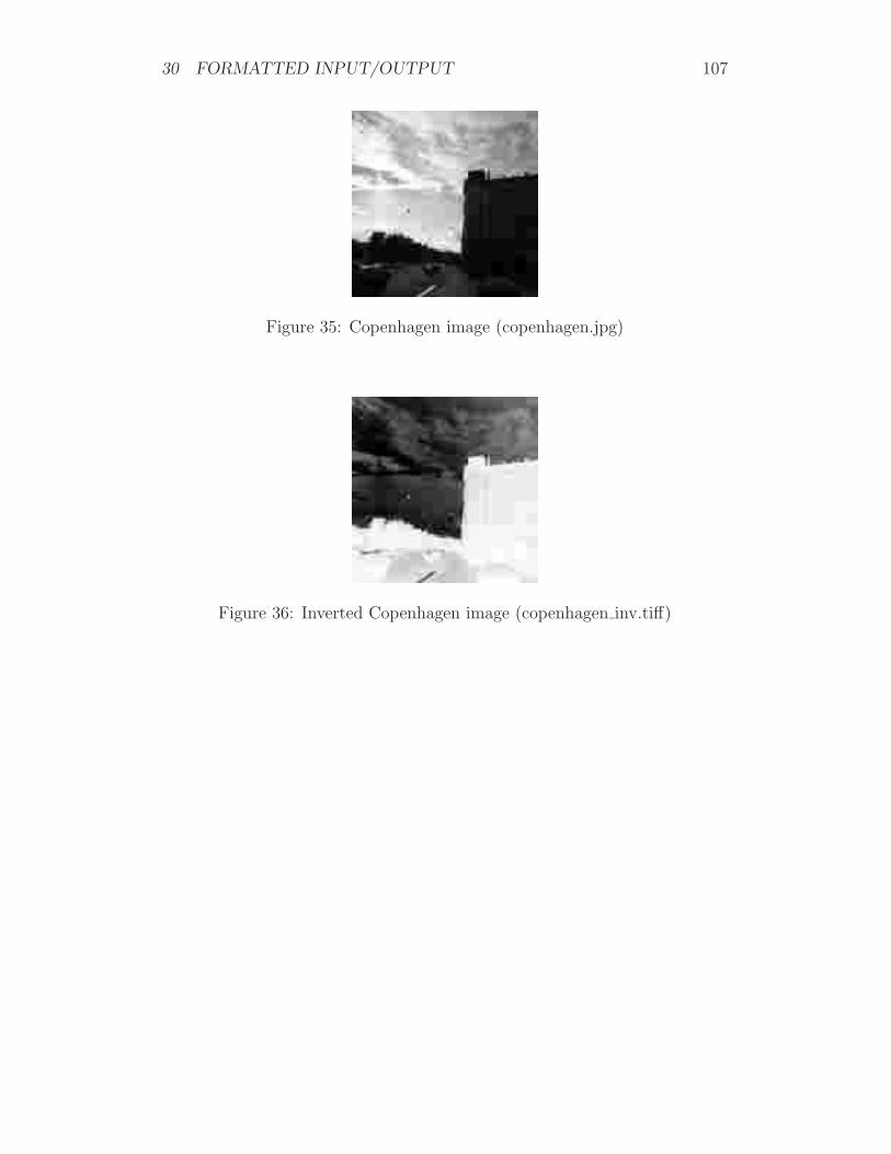
30 FORMATTED INPUT/OUTPUT 107
Figure 35: Copenhagen image (copenhagen.jpg)
Figure 36: Inverted Copenhagen image (copenhagen inv.tiff)
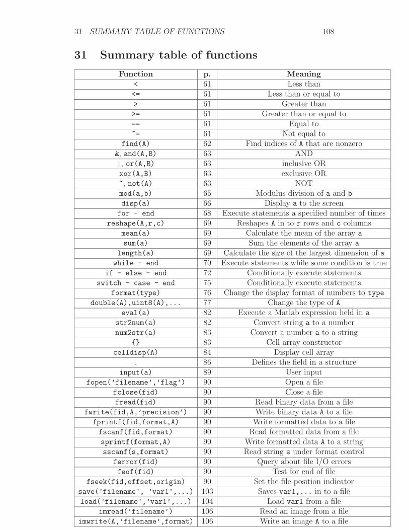
31 SUMMARY TABLE OF FUNCTIONS 108
31 Summary table of functions
Function p. Meaning< 61 Less than<= 61 Less than or equal to> 61 Greater than>= 61 Greater than or equal to== 61 Equal to~= 61 Not equal to
find(A) 62 Find indices of A that are nonzero&, and(A,B) 63 AND|, or(A,B) 63 inclusive ORxor(A,B) 63 exclusive OR~, not(A) 63 NOTmod(a,b) 65 Modulus division of a and b
disp(a) 66 Display a to the screenfor - end 68 Execute statements a specified number of times
reshape(A,r,c) 69 Reshapes A in to r rows and c columnsmean(a) 69 Calculate the mean of the array a
sum(a) 69 Sum the elements of the array a
length(a) 69 Calculate the size of the largest dimension of awhile - end 70 Execute statements while some condition is true
if - else - end 72 Conditionally execute statementsswitch - case - end 75 Conditionally execute statements
format(type) 76 Change the display format of numbers to type
double(A),uint8(A),... 77 Change the type of Aeval(a) 82 Execute a Matlab expression held in a
str2num(a) 82 Convert string a to a numbernum2str(a) 83 Convert a number a to a string
{} 83 Cell array constructorcelldisp(A) 84 Display cell array
. 86 Defines the field in a structureinput(a) 89 User input
fopen(’filename’,’flag’) 90 Open a filefclose(fid) 90 Close a filefread(fid) 90 Read binary data from a file
fwrite(fid,A,’precision’) 90 Write binary data A to a filefprintf(fid,format,A) 90 Write formatted data to a filefscanf(fid,format) 90 Read formatted data from a filesprintf(format,A) 90 Write formatted data A to a stringsscanf(s,format) 90 Read string s under format control
ferror(fid) 90 Query about file I/O errorsfeof(fid) 90 Test for end of file
fseek(fid,offset,origin) 90 Set the file position indicatorsave(’filename’, ’var1’,...) 103 Saves var1,... in to a fileload(’filename’,’var1’,...) 104 Load var1 from a file
imread(’filename’) 106 Read an image from a fileimwrite(A,’filename’,format) 106 Write an image A to a file
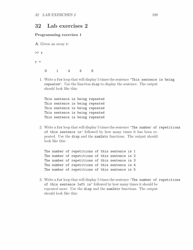
32 LAB EXERCISES 2 109
32 Lab exercises 2
Programming exercises 1
A. Given an array r:
>> r
r =
9 1 4 6 8
1. Write a for loop that will display 5 times the sentence ’This sentence is being
repeated’. Use the function disp to display the sentence. The outputshould look like this:
This sentence is being repeated
This sentence is being repeated
This sentence is being repeated
This sentence is being repeated
This sentence is being repeated
2. Write a for loop that will display 5 times the sentence ’The number of repetitions
of this sentence is’ followed by how many times it has been re-peated. Use the disp and the num2str functions. The output shouldlook like this:
The number of repetitions of this sentence is 1
The number of repetitions of this sentence is 2
The number of repetitions of this sentence is 3
The number of repetitions of this sentence is 4
The number of repetitions of this sentence is 5
3. Write a for loop that will display 5 times the sentence ’The number of repetitions
of this sentence left is’ followed by how many times it should berepeated more. Use the disp and the num2str functions. The outputshould look like this:

32 LAB EXERCISES 2 110
The number of repetitions of this sentence left is 4
The number of repetitions of this sentence left is 3
The number of repetitions of this sentence left is 2
The number of repetitions of this sentence left is 1
The number of repetitions of this sentence left is 0
4. Write a for loop that will display all the elements of the array r one ata time (starting with the first element (9) and finishing with the lastelement (8)).
5. Write a for loop that will display all the elements of the array r one ata time in reverse order (starting with the last element (8) and finishingwith the first one (9)).
6. Write a for loop that will display elements of r that are larger than 5.Use if-else to check if an element of r is larger than 5.
7. Repeat the previous using a while loop instead of a for loop.
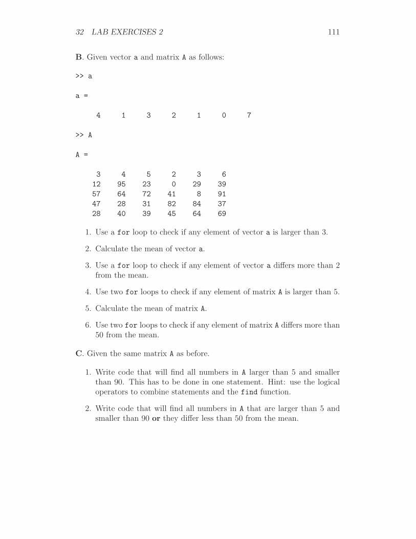
32 LAB EXERCISES 2 111
B. Given vector a and matrix A as follows:
>> a
a =
4 1 3 2 1 0 7
>> A
A =
3 4 5 2 3 6
12 95 23 0 29 39
57 64 72 41 8 91
47 28 31 82 84 37
28 40 39 45 64 69
1. Use a for loop to check if any element of vector a is larger than 3.
2. Calculate the mean of vector a.
3. Use a for loop to check if any element of vector a differs more than 2from the mean.
4. Use two for loops to check if any element of matrix A is larger than 5.
5. Calculate the mean of matrix A.
6. Use two for loops to check if any element of matrix A differs more than50 from the mean.
C. Given the same matrix A as before.
1. Write code that will find all numbers in A larger than 5 and smallerthan 90. This has to be done in one statement. Hint: use the logicaloperators to combine statements and the find function.
2. Write code that will find all numbers in A that are larger than 5 andsmaller than 90 or they differ less than 50 from the mean.
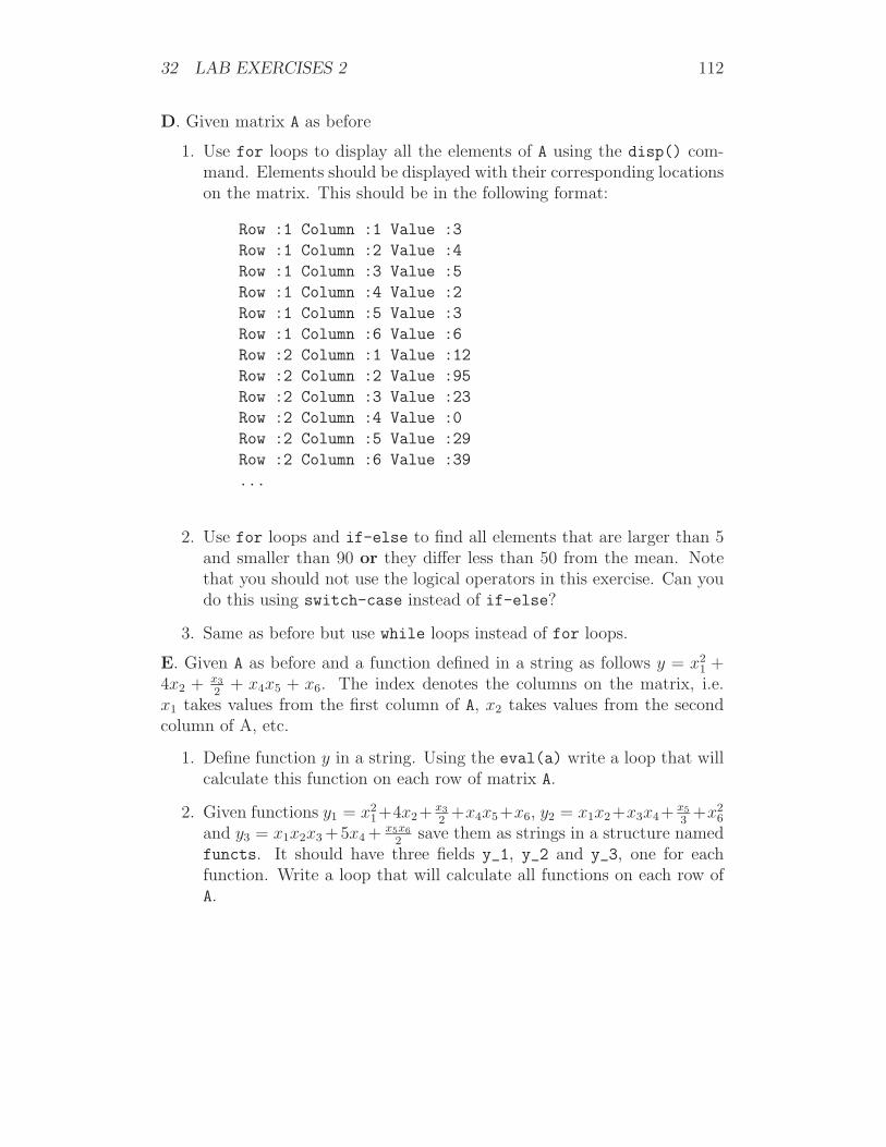
32 LAB EXERCISES 2 112
D. Given matrix A as before
1. Use for loops to display all the elements of A using the disp() com-mand. Elements should be displayed with their corresponding locationson the matrix. This should be in the following format:
Row :1 Column :1 Value :3
Row :1 Column :2 Value :4
Row :1 Column :3 Value :5
Row :1 Column :4 Value :2
Row :1 Column :5 Value :3
Row :1 Column :6 Value :6
Row :2 Column :1 Value :12
Row :2 Column :2 Value :95
Row :2 Column :3 Value :23
Row :2 Column :4 Value :0
Row :2 Column :5 Value :29
Row :2 Column :6 Value :39
...
2. Use for loops and if-else to find all elements that are larger than 5and smaller than 90 or they differ less than 50 from the mean. Notethat you should not use the logical operators in this exercise. Can youdo this using switch-case instead of if-else?
3. Same as before but use while loops instead of for loops.
E. Given A as before and a function defined in a string as follows y = x21 +
4x2 + x3
2+ x4x5 + x6. The index denotes the columns on the matrix, i.e.
x1 takes values from the first column of A, x2 takes values from the secondcolumn of A, etc.
1. Define function y in a string. Using the eval(a) write a loop that willcalculate this function on each row of matrix A.
2. Given functions y1 = x21+4x2+
x3
2+x4x5+x6, y2 = x1x2+x3x4+
x5
3+x2
6
and y3 = x1x2x3 +5x4 + x5x6
2save them as strings in a structure named
functs. It should have three fields y_1, y_2 and y_3, one for eachfunction. Write a loop that will calculate all functions on each row ofA.
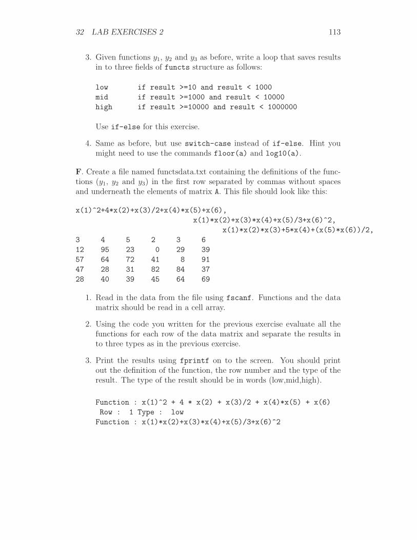
32 LAB EXERCISES 2 113
3. Given functions y1, y2 and y3 as before, write a loop that saves resultsin to three fields of functs structure as follows:
low if result >=10 and result < 1000
mid if result >=1000 and result < 10000
high if result >=10000 and result < 1000000
Use if-else for this exercise.
4. Same as before, but use switch-case instead of if-else. Hint youmight need to use the commands floor(a) and log10(a).
F. Create a file named functsdata.txt containing the definitions of the func-tions (y1, y2 and y3) in the first row separated by commas without spacesand underneath the elements of matrix A. This file should look like this:
x(1)^2+4*x(2)+x(3)/2+x(4)*x(5)+x(6),
x(1)*x(2)+x(3)*x(4)+x(5)/3+x(6)^2,
x(1)*x(2)*x(3)+5*x(4)+(x(5)*x(6))/2,
3 4 5 2 3 6
12 95 23 0 29 39
57 64 72 41 8 91
47 28 31 82 84 37
28 40 39 45 64 69
1. Read in the data from the file using fscanf. Functions and the datamatrix should be read in a cell array.
2. Using the code you written for the previous exercise evaluate all thefunctions for each row of the data matrix and separate the results into three types as in the previous exercise.
3. Print the results using fprintf on to the screen. You should printout the definition of the function, the row number and the type of theresult. The type of the result should be in words (low,mid,high).
Function : x(1)^2 + 4 * x(2) + x(3)/2 + x(4)*x(5) + x(6)
Row : 1 Type : low
Function : x(1)*x(2)+x(3)*x(4)+x(5)/3+x(6)^2
32 LAB EXERCISES 2 114
Row : 1 Type : low
Function : x(1)*x(2)*x(3)+5*x(4)+(x(5)*x(6))/2
Row : 1 Type : low
Function : x(1)^2 + 4 * x(2) + x(3)/2 + x(4)*x(5) + x(6)
Row : 2 Type : low
Function : x(1)*x(2)+x(3)*x(4)+x(5)/3+x(6)^2
Row : 2 Type : mid
...
4. Print the results in a file named results.txt.
5. Print the results in to three files named results1.txt, results2.txt andresults3.txt. Each file should contain results of one type (low,mid,high).You might need to use the ’a’ flag in the command fopen(filename,’a’).This flag will open (or create if it does not exist) a file, keep the contentsand append data to the end of the file.
6. Repeat the previous exercise without using any conditional operators(if-else,switch-case).
G. Given any gray scale JPEG image.
1. Read it in using imread
2. Rotate the image 90 degrees clockwise.
3. Write the rotated image in to a JPEG file using imwrite.
32 LAB EXERCISES 2 115
Questions from the lecture
1. How can we simplify the next example and avoid using a for loop?
>> x_values = [0:0.1:2*pi - 0.1];
>> for index=1:length(x_values)
y_values(index) = sin(x_values(index));
end
2. How can the next example be accomplished using the command find()?
>> A = zeros(10,1);
>> A(5) = 1;
>> m = 1;
>> while A(m) == 0
m = m + 1;
end
>> m
m =
5
3. How can we accomplish the next function without using if-else andfor loop in three statements?
function [div_2, div_3, not_div] = myseparate(A)
% rtn = mysort(A) takes a scalar vector as input
% and sorts it out to numbers that are divisible by 2 (div_2),
% numbers that are divisible by 3 (div_3) and
% other numbers that are not divisible by 2 or 3.
% If a number is divisible by 2 and 3 then it will go to both lists.
count_div_2 = 0; count_div_3 = 0; count_not_div = 0;
for m=1:length(A)
if mod(A(m),2) == 0 & mod(A(m),3) == 0
32 LAB EXERCISES 2 116
count_div_2 = count_div_2 + 1;
div_2(count_div_2) = A(m);
count_div_3 = count_div_3 + 1;
div_3(count_div_3) = A(m);
elseif mod(A(m),2) == 0
count_div_2 = count_div_2 + 1;
div_2(count_div_2) = A(m);
elseif mod(A(m),3) == 0
count_div_3 = count_div_3 + 1;
div_3(count_div_3) = A(m);
else
count_not_div = count_not_div + 1;
not_div(count_not_div) = A(m);
end
end
32 LAB EXERCISES 2 117
Programming exercises 2
Aim: The aim of this exercise is to implement linear regression with basisfunctions and to visualize the phenomena of overfitting.
Linear regression overview: Given a set of data:
{(x1, y1), (x2, y2), . . . , (xℓ, yℓ)} (7)
where x = (x1, . . . , xn) is a vector in ℜn and y is a real number. Linearregression finds a vector u ∈ ℜn such that the sum of squared errors
SSE =ℓ∑
t=1
(yt − u · xt)2 (8)
is minimized. This is expressible in matrix form by defining X to be the ℓ×n
matrix
X =
x1,1 x1,2 . . . x1,n
x2,1 x2,2 . . . x2,n
......
. . ....
xℓ,1 xℓ,2 . . . xℓ,n
, (9)
and defining y to be the column vector y = (y1, . . . , yℓ). The vector u thenminimizes
(Xu − y)T (Xu − y).
In linear regression with basis functions we fit the data sequence with alinear combination of basis functions (f1, f2, . . ., fk). This is done by trans-forming the data as follows
{((f1(x1), . . . , fk(x1)), y1), . . . , ((f1(xℓ), . . . , fk(xℓ)), yℓ)}, (10)
and then applying linear regression above to this transformed data set. Linearregression on the transformed dataset thus finds a k-dimensional vector u =(u1, . . . , uk) such that
ℓ∑
t=1
(yt −k∑
i=1
uifi(xt))2 (11)
is minimized.A common basis used in practice is a polynomial basis {1, x, x2, x3, . . . , xk−1}
of dimension k (order k − 1) in the figure below we give a simple fit of fourpoints produced by a linear (k = 2) and cubic (k = 4) polynomial.
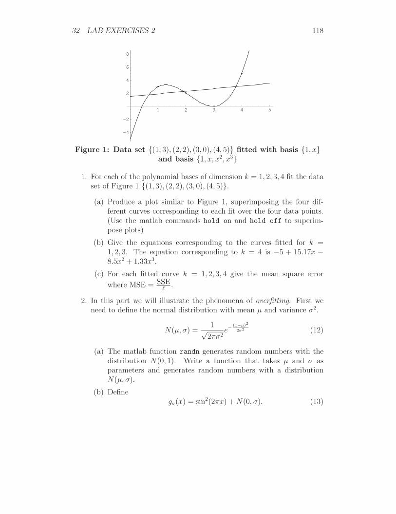
32 LAB EXERCISES 2 118
1 2 3 4 5
-4
-2
2
4
6
8
Figure 1: Data set {(1, 3), (2, 2), (3, 0), (4, 5)} fitted with basis {1, x}and basis {1, x, x2, x3}
1. For each of the polynomial bases of dimension k = 1, 2, 3, 4 fit the dataset of Figure 1 {(1, 3), (2, 2), (3, 0), (4, 5)}.
(a) Produce a plot similar to Figure 1, superimposing the four dif-ferent curves corresponding to each fit over the four data points.(Use the matlab commands hold on and hold off to superim-pose plots)
(b) Give the equations corresponding to the curves fitted for k =1, 2, 3. The equation corresponding to k = 4 is −5 + 15.17x −8.5x2 + 1.33x3.
(c) For each fitted curve k = 1, 2, 3, 4 give the mean square error
where MSE = SSEℓ
.
2. In this part we will illustrate the phenomena of overfitting. First weneed to define the normal distribution with mean µ and variance σ2.
N(µ, σ) =1√
2πσ2e−
(x−µ)2
2σ2 (12)
(a) The matlab function randn generates random numbers with thedistribution N(0, 1). Write a function that takes µ and σ asparameters and generates random numbers with a distributionN(µ, σ).
(b) Definegσ(x) = sin2(2πx) + N(0, σ). (13)

32 LAB EXERCISES 2 119
sample uniformly at random from the interval [0, 1] 30 times cre-ating (x1, . . . , x30) and apply g0.07 to each x creating the data set
S0.07,30 = {(x1, g0.07(x1)), . . . , (x30, g0.07(x30)}. (14)
i. Plot the function sin2(2πx) from x = 0..1 with the points ofthe above data set superimposed. The plot should resemble
0.2 0.4 0.6 0.8 1
0.2
0.4
0.6
0.8
1
ii. Fit the data set with a polynomial bases of dimension k =2, 5, 10, 15, 20 plot each of these 5 curves superimposed over aplot of data points.
(c) Let the training error tek(S) denote the MSE of the fitting of thedata set S with polynomial basis of dimension k. Plot the log ofthe training error versus the polynomial dimension k = 1, . . . , 25(this should be a decreasing function).
(d) Generate a test set T of a thousand points,
T0.07,1000 = {(x1, g0.07(x1)), . . . , (x1000, g0.07(x1000)}. (15)
Define the test error tsek(S, T ) to be the MSE of the test setT on the polynomial of dimension k fitted from training set S.Plot the log of the test error versus the polynomial dimensionk = 1, . . . , 20. Unlike the training error this is not a decreasingfunction. This is the phenomena of overfitting. Although thetraining error decreases with growing k the test error eventuallyincreases since rather than fitting the function, in a loose sense,we begin to fit to the noise.
(e) For any given set of random numbers we will get slightly differenttraining curves and test curves. It is instructive to see these curves
32 LAB EXERCISES 2 120
smoothed out. For this part repeat items (c) and (d) but insteadof plotting the results of a single “run” plot the average results ofa 100 runs (note: plot the log(avg) rather than the avg(log)).
3. In this part we will use as a basis
sin(1πx), sin(2πx), sin(3πx), . . . , sin(kπx).
Repeat the experiments in 2 (c-e) with the above basis.
121
Part IV
Lecture 3
33 Overview of Lecture 3
• Matlab performance tuning
• Set functions
• User defined functions 2
• Plotting 2
• Summary table of functions
34 MATLAB PERFORMANCE TUNING 122
34 Matlab performance tuning
In order to assess the performance of our code we can use Matlab’s profiler.The profiler gives details in html format of how much time was spent on eachfunction and how many times a functions was called. To enable the profilerwe must type profile on at the beginning of our code. To produce thehtml report we will need to type profile report at the end of our code. Toswitch off the profiler we will type profile off. Next is an example thatuses a user defined function graddesc for gradient descent. This functionuses another function called dfb.
>> profile on
>> sol = graddesc(’fb’, ’dfb’, [0.0 0.0], 0.001, 0.001);
>> profile report
>> profile off
>> profile resume % restarts profiler
>> profile clear % clears profiler
The command profile resume will resume the profiler and profile clear
will clear all the data that the profiler saved. The resulting report from theprofiler is shown in fig. 37. We can use this information to see how muchtime is spent on each function and determine inefficiencies in our code. Notethat on the top of the summary report, the precision of the clock is displayed.Any time lower than that will be displayed as 0.
A simpler way to time our functions is to use a pair of the commands ticand toc.
Command Meaningtic Starts timertoc Returns time
We will type tic immediately before our function and then type toc imme-diately after the function.
>> tic; a = [1:1000000]; toc
elapsed_time =
0.1210

34 MATLAB PERFORMANCE TUNING 123
Figure 37: Profile Report: Summary
Consider a simple example that calculates the sin function for 10000points.
>> m = []; y_vals = []; % clears the variables
>> tic; for m=1:10000
y_vals(m) = sin(m);
end;toc
elapsed_time =
0.8010
The first thing we can do to speed up our code is to preallocate arrays.

34 MATLAB PERFORMANCE TUNING 124
Figure 38: Profile Report: Function details
>> m = []; y_vals = [];
>> tic; y_vals = zeros(1,10000); for m=1:10000
y_vals(m) = sin(m);
end;toc
elapsed_time =
0.0700
The second thing and most important is to vectorize the loop.
>> m = []; y_vals = [];
>> tic; m = 1:10000 ; y_vals(m) = sin(m);toc

34 MATLAB PERFORMANCE TUNING 125
elapsed_time =
0.0100
Loops in Matlab are very time consuming and should be vectorized whenpossible. Using array preallocation and vectorization we achieved 80 timesspeedup.
Method TimeSimple 0.8010
Preallocation 0.0700Preallocation and vectorization 0.0100
To further improve the performance of our code, we can use sparse matri-ces. A sparse matrix stores only the non-zero elements. As well as reducingmemory requirements, there are special algorithms for sparse matrices whichrun faster than the equivalent full matrix. Sparse matrices make a noticeabledifference if we use large matrices with many elements equal to zero. To ini-tialize a sparse matrix we will use the function sparse(a,b), which createsan a x b sparse matrix.
>> A = sparse(10,10);
>> A
A =
All zero sparse: 10-by-10
>> B = eye(10);
>> B_spar = sparse(B);
>> whos B
Name Size Bytes Class
B 10x10 800 double array
Grand total is 100 elements using 800 bytes
>> whos B_spar
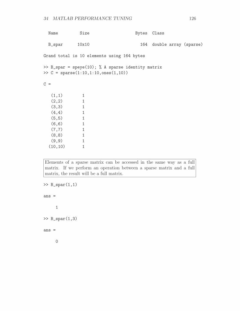
34 MATLAB PERFORMANCE TUNING 126
Name Size Bytes Class
B_spar 10x10 164 double array (sparse)
Grand total is 10 elements using 164 bytes
>> B_spar = speye(10); % A sparse identity matrix
>> C = sparse(1:10,1:10,ones(1,10))
C =
(1,1) 1
(2,2) 1
(3,3) 1
(4,4) 1
(5,5) 1
(6,6) 1
(7,7) 1
(8,8) 1
(9,9) 1
(10,10) 1
Elements of a sparse matrix can be accessed in the same way as a fullmatrix. If we perform an operation between a sparse matrix and a fullmatrix, the result will be a full matrix.
>> B_spar(1,1)
ans =
1
>> B_spar(1,3)
ans =
0
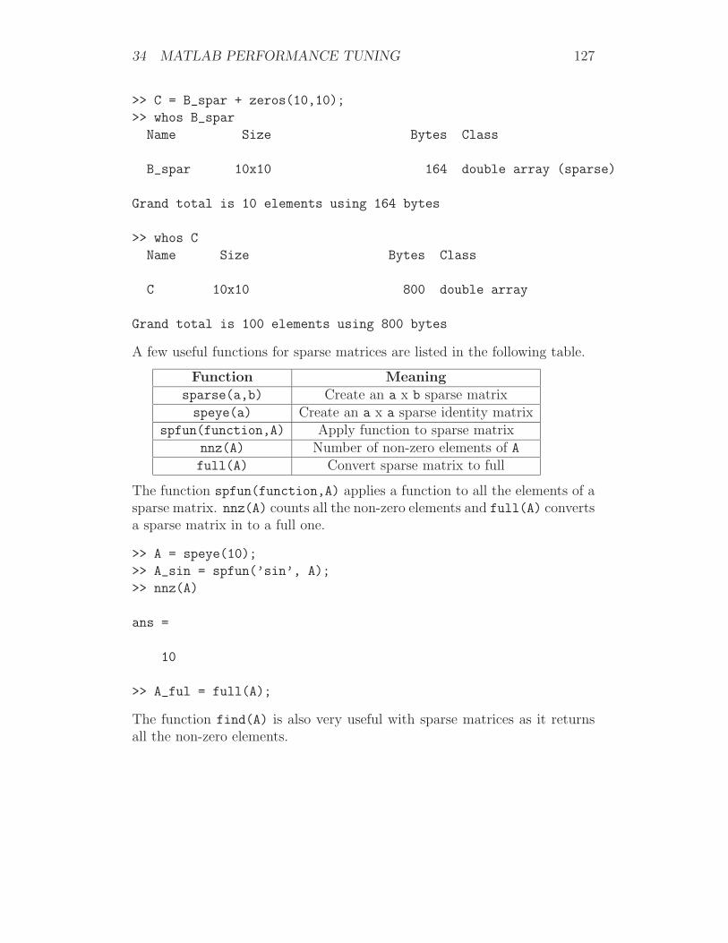
34 MATLAB PERFORMANCE TUNING 127
>> C = B_spar + zeros(10,10);
>> whos B_spar
Name Size Bytes Class
B_spar 10x10 164 double array (sparse)
Grand total is 10 elements using 164 bytes
>> whos C
Name Size Bytes Class
C 10x10 800 double array
Grand total is 100 elements using 800 bytes
A few useful functions for sparse matrices are listed in the following table.
Function Meaningsparse(a,b) Create an a x b sparse matrixspeye(a) Create an a x a sparse identity matrix
spfun(function,A) Apply function to sparse matrixnnz(A) Number of non-zero elements of Afull(A) Convert sparse matrix to full
The function spfun(function,A) applies a function to all the elements of asparse matrix. nnz(A) counts all the non-zero elements and full(A) convertsa sparse matrix in to a full one.
>> A = speye(10);
>> A_sin = spfun(’sin’, A);
>> nnz(A)
ans =
10
>> A_ful = full(A);
The function find(A) is also very useful with sparse matrices as it returnsall the non-zero elements.
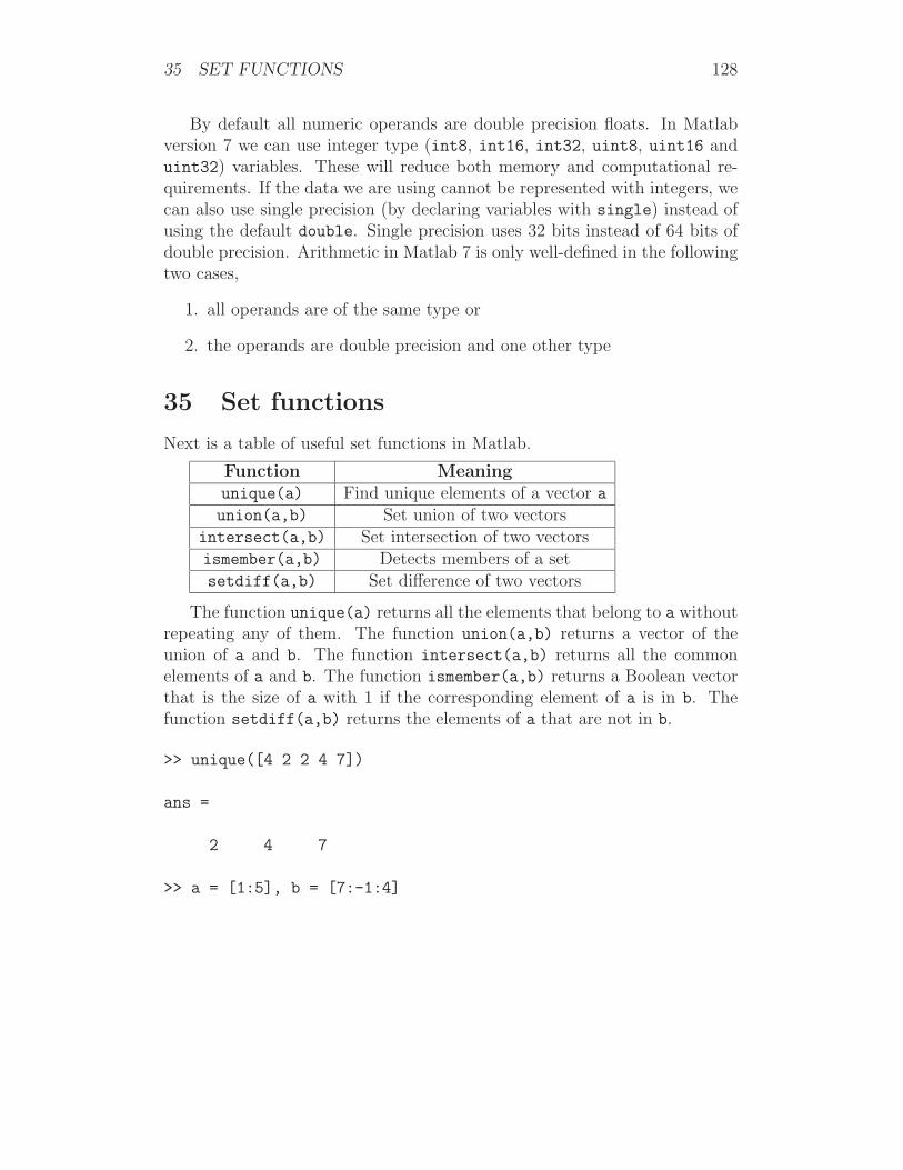
35 SET FUNCTIONS 128
By default all numeric operands are double precision floats. In Matlabversion 7 we can use integer type (int8, int16, int32, uint8, uint16 anduint32) variables. These will reduce both memory and computational re-quirements. If the data we are using cannot be represented with integers, wecan also use single precision (by declaring variables with single) instead ofusing the default double. Single precision uses 32 bits instead of 64 bits ofdouble precision. Arithmetic in Matlab 7 is only well-defined in the followingtwo cases,
1. all operands are of the same type or
2. the operands are double precision and one other type
35 Set functions
Next is a table of useful set functions in Matlab.
Function Meaningunique(a) Find unique elements of a vector aunion(a,b) Set union of two vectors
intersect(a,b) Set intersection of two vectorsismember(a,b) Detects members of a setsetdiff(a,b) Set difference of two vectors
The function unique(a) returns all the elements that belong to a withoutrepeating any of them. The function union(a,b) returns a vector of theunion of a and b. The function intersect(a,b) returns all the commonelements of a and b. The function ismember(a,b) returns a Boolean vectorthat is the size of a with 1 if the corresponding element of a is in b. Thefunction setdiff(a,b) returns the elements of a that are not in b.
>> unique([4 2 2 4 7])
ans =
2 4 7
>> a = [1:5], b = [7:-1:4]
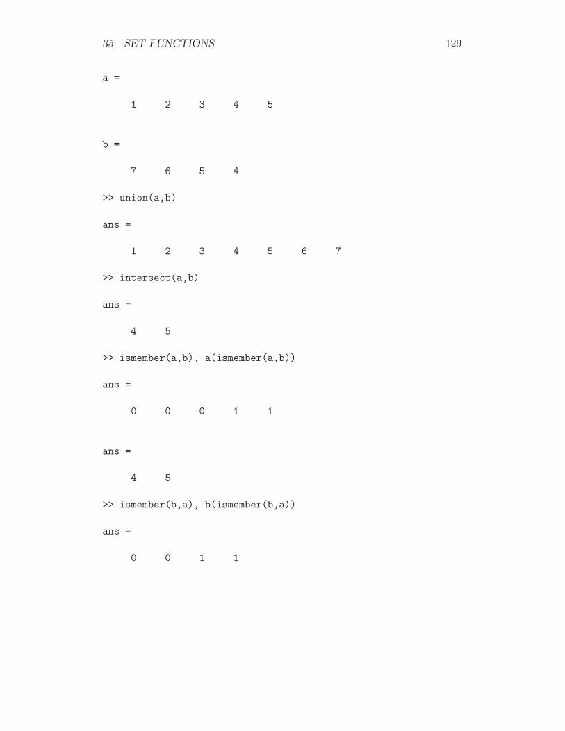
35 SET FUNCTIONS 129
a =
1 2 3 4 5
b =
7 6 5 4
>> union(a,b)
ans =
1 2 3 4 5 6 7
>> intersect(a,b)
ans =
4 5
>> ismember(a,b), a(ismember(a,b))
ans =
0 0 0 1 1
ans =
4 5
>> ismember(b,a), b(ismember(b,a))
ans =
0 0 1 1
36 USER DEFINED FUNCTIONS 2 130
ans =
5 4
>> setdiff(a,b), setdiff(b,a)
ans =
1 2 3
ans =
6 7
36 User defined functions 2
Variables inside functions are by default local, that means only the function,where the variables were declared, can access them and as soon as thefunction terminates they are deleted from memory. We can also definevariables inside a function to be global or persistent. persistent variablescan only be accessed from the function they are declared in, but they persistin memory between function calls. global variables are both persistentand they can be accessed by other functions which declare them global.
As an example we have created two functions mytic and mytoc:
function mytic
global my_time
my_time = cputime;
function rtn = mytoc
global my_time
36 USER DEFINED FUNCTIONS 2 131
rtn = cputime - my_time;
Then we can type on the command prompt:
>> m = [];
>> mytic;m=1:100000;sin(m);mytoc
ans =
0.0700
Next is an example of a persistent variable. The next function is calledcounter
function rtn = counter
persistent count
if isempty(count)
count = 1;
else
count = count + 1;
end
rtn = count;
The function isempty(A) tests whether the variable held in A has been cre-ated or not. On the command prompt we will type:
>> counter
ans =
1
>> counter
ans =
36 USER DEFINED FUNCTIONS 2 132
2
We can also create functions from strings via inline(expr_string,arg1,arg2,...),where expr_string is a string which defines the function and arg1, arg2,... are strings naming the arguments of the function.
>> h = inline(’A+2*B+4*C’,’A’,’B’,’C’)
h =
Inline function:
h(A,B,C) = A+2*B+4*C
>> h([1 0 ; 0 1],[1 0 ; 0 1],[0 1 ; 1 0])
ans =
3 4
4 3
>> g = inline(’(x(1)-5).^2 + 3*(x(2)-2).^2’,’x’)
g =
Inline function:
g(x) = (x(1)-5).^2 + 3*(x(2)-2).^2
>> g([1 , 2]), g([5 , 2])
ans =
16
ans =
0
36 USER DEFINED FUNCTIONS 2 133
The number of arguments in a function does not need to be predeter-mined. We can use varargin as an argument that means we can have avariable number of arguments of any type. To determine how many argu-ments the user passed to the function we will use nargin. Note that nargincounts the total number of input arguments, not just the ones correspondingto varargin. The following example is a function that prints any number ofarguments on to the screen.
function print_various_arguments(head, varargin)
for m=1:nargin-1
fprintf(1,head,m);
disp(varargin{m});
end
Then on the command prompt we type:
>> print_various_arguments(’arg %d is ’,7,[1 2 3],’a string’)
arg 1 is 7
arg 2 is 1 2 3
arg 3 is a string
The examples print_data_screen and print_data_file in the previousset of notes can be combined using varargin. The new function can take 3or 4 arguments which determines whether it prints to the screen or to a file.
function print_data(column_name, row_name, data_row,varargin)
% function print_data(column_name, row_name, data_row,varargin)
if nargin == 3
fid = 1;
elseif nargin == 4
filename = varargin{1};
fid = fopen(filename,’w’);
end
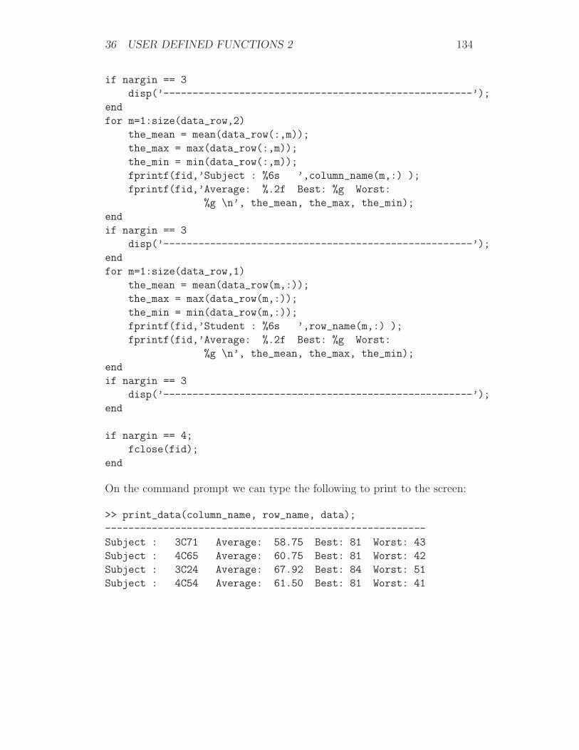
36 USER DEFINED FUNCTIONS 2 134
if nargin == 3
disp(’-----------------------------------------------------’);
end
for m=1:size(data_row,2)
the_mean = mean(data_row(:,m));
the_max = max(data_row(:,m));
the_min = min(data_row(:,m));
fprintf(fid,’Subject : %6s ’,column_name(m,:) );
fprintf(fid,’Average: %.2f Best: %g Worst:
%g \n’, the_mean, the_max, the_min);
end
if nargin == 3
disp(’-----------------------------------------------------’);
end
for m=1:size(data_row,1)
the_mean = mean(data_row(m,:));
the_max = max(data_row(m,:));
the_min = min(data_row(m,:));
fprintf(fid,’Student : %6s ’,row_name(m,:) );
fprintf(fid,’Average: %.2f Best: %g Worst:
%g \n’, the_mean, the_max, the_min);
end
if nargin == 3
disp(’-----------------------------------------------------’);
end
if nargin == 4;
fclose(fid);
end
On the command prompt we can type the following to print to the screen:
>> print_data(column_name, row_name, data);
-------------------------------------------------------
Subject : 3C71 Average: 58.75 Best: 81 Worst: 43
Subject : 4C65 Average: 60.75 Best: 81 Worst: 42
Subject : 3C24 Average: 67.92 Best: 84 Worst: 51
Subject : 4C54 Average: 61.50 Best: 81 Worst: 41
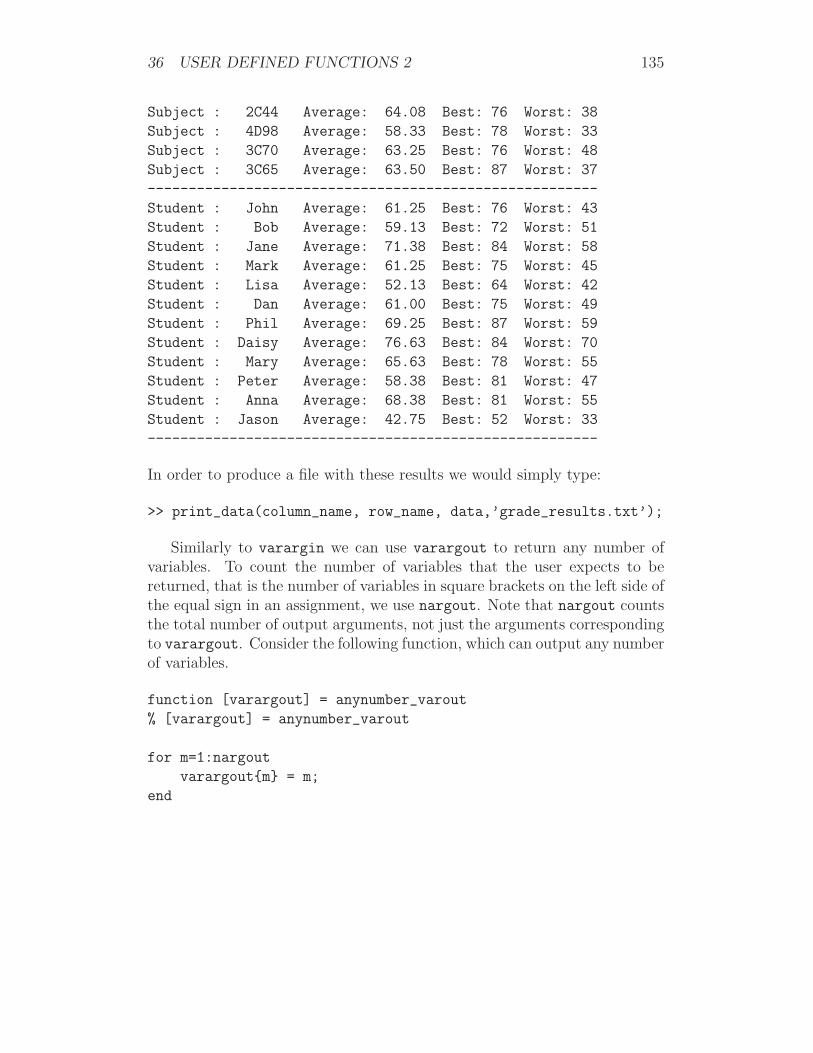
36 USER DEFINED FUNCTIONS 2 135
Subject : 2C44 Average: 64.08 Best: 76 Worst: 38
Subject : 4D98 Average: 58.33 Best: 78 Worst: 33
Subject : 3C70 Average: 63.25 Best: 76 Worst: 48
Subject : 3C65 Average: 63.50 Best: 87 Worst: 37
-------------------------------------------------------
Student : John Average: 61.25 Best: 76 Worst: 43
Student : Bob Average: 59.13 Best: 72 Worst: 51
Student : Jane Average: 71.38 Best: 84 Worst: 58
Student : Mark Average: 61.25 Best: 75 Worst: 45
Student : Lisa Average: 52.13 Best: 64 Worst: 42
Student : Dan Average: 61.00 Best: 75 Worst: 49
Student : Phil Average: 69.25 Best: 87 Worst: 59
Student : Daisy Average: 76.63 Best: 84 Worst: 70
Student : Mary Average: 65.63 Best: 78 Worst: 55
Student : Peter Average: 58.38 Best: 81 Worst: 47
Student : Anna Average: 68.38 Best: 81 Worst: 55
Student : Jason Average: 42.75 Best: 52 Worst: 33
-------------------------------------------------------
In order to produce a file with these results we would simply type:
>> print_data(column_name, row_name, data,’grade_results.txt’);
Similarly to varargin we can use varargout to return any number ofvariables. To count the number of variables that the user expects to bereturned, that is the number of variables in square brackets on the left side ofthe equal sign in an assignment, we use nargout. Note that nargout countsthe total number of output arguments, not just the arguments correspondingto varargout. Consider the following function, which can output any numberof variables.
function [varargout] = anynumber_varout
% [varargout] = anynumber_varout
for m=1:nargout
varargout{m} = m;
end
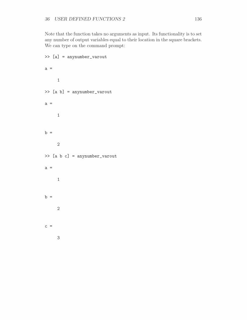
36 USER DEFINED FUNCTIONS 2 136
Note that the function takes no arguments as input. Its functionality is to setany number of output variables equal to their location in the square brackets.We can type on the command prompt:
>> [a] = anynumber_varout
a =
1
>> [a b] = anynumber_varout
a =
1
b =
2
>> [a b c] = anynumber_varout
a =
1
b =
2
c =
3
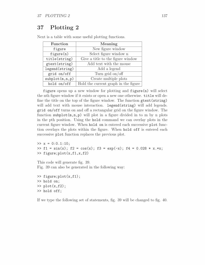
37 PLOTTING 2 137
37 Plotting 2
Next is a table with some useful plotting functions.
Function Meaningfigure New figure window
figure(n) Select figure window ntitle(string) Give a title to the figure windowgtext(string) Add text with the mouselegend(string) Add a legendgrid on/off Turn grid on/off
subplot(m,n,p) Create multiple plotshold on/off Hold the current graph in the figure
figure opens up a new window for plotting and figure(n) will selectthe nth figure window if it exists or open a new one otherwise. title will de-fine the title on the top of the figure window. The function gtext(string)
will add text with mouse interaction. legend(string) will add legends.grid on/off turns on and off a rectangular grid on the figure window. Thefunction subplot(m,n,p) will plot in a figure divided in to m by n plotsin the pth position. Using the hold command we can overlay plots in thecurrent figure window. When hold on is entered each successive plot func-tion overlays the plots within the figure. When hold off is entered eachsuccessive plot function replaces the previous plot.
>> x = 0:0.1:10;
>> f1 = sin(x); f2 = cos(x); f3 = exp(-x); f4 = 0.028 * x.*x;
>> figure;plot(x,f1,x,f2)
This code will generate fig. 39.Fig. 39 can also be generated in the following way:
>> figure;plot(x,f1);
>> hold on;
>> plot(x,f2);
>> hold off;
If we type the following set of statements, fig. 39 will be changed to fig. 40.
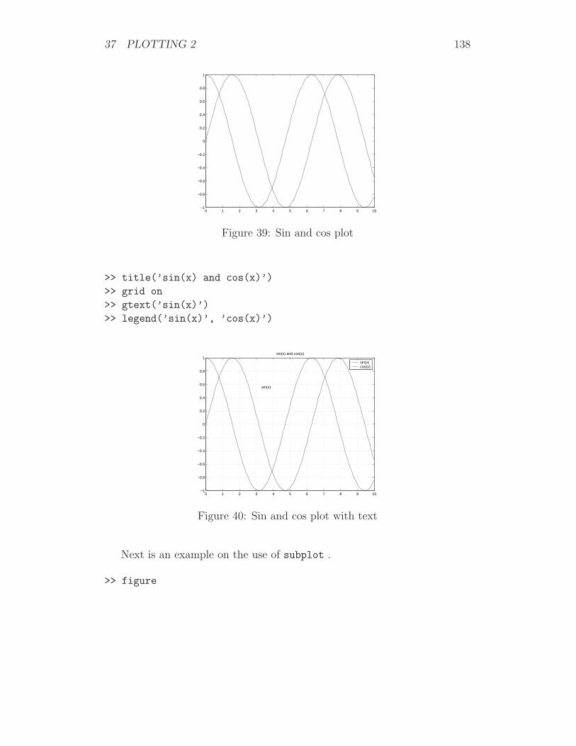
37 PLOTTING 2 138
0 1 2 3 4 5 6 7 8 9 10−1
−0.8
−0.6
−0.4
−0.2
0
0.2
0.4
0.6
0.8
1
Figure 39: Sin and cos plot
>> title(’sin(x) and cos(x)’)
>> grid on
>> gtext(’sin(x)’)
>> legend(’sin(x)’, ’cos(x)’)
0 1 2 3 4 5 6 7 8 9 10−1
−0.8
−0.6
−0.4
−0.2
0
0.2
0.4
0.6
0.8
1sin(x) and cos(x)
sin(x)
sin(x)cos(x)
Figure 40: Sin and cos plot with text
Next is an example on the use of subplot .
>> figure
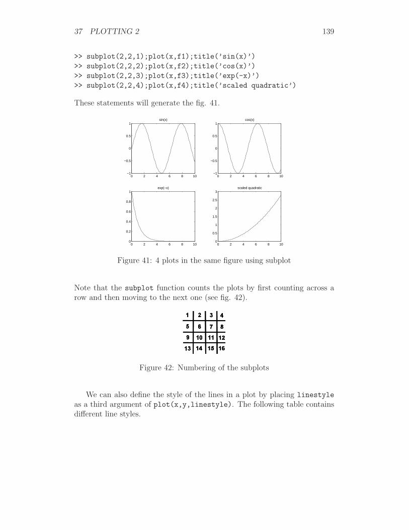
37 PLOTTING 2 139
>> subplot(2,2,1);plot(x,f1);title(’sin(x)’)
>> subplot(2,2,2);plot(x,f2);title(’cos(x)’)
>> subplot(2,2,3);plot(x,f3);title(’exp(-x)’)
>> subplot(2,2,4);plot(x,f4);title(’scaled quadratic’)
These statements will generate the fig. 41.
0 2 4 6 8 10−1
−0.5
0
0.5
1sin(x)
0 2 4 6 8 10−1
−0.5
0
0.5
1cos(x)
0 2 4 6 8 100
0.2
0.4
0.6
0.8
1exp(−x)
0 2 4 6 8 100
0.5
1
1.5
2
2.5
3scaled quadratic
Figure 41: 4 plots in the same figure using subplot
Note that the subplot function counts the plots by first counting across arow and then moving to the next one (see fig. 42).
Figure 42: Numbering of the subplots
We can also define the style of the lines in a plot by placing linestyle
as a third argument of plot(x,y,linestyle). The following table containsdifferent line styles.
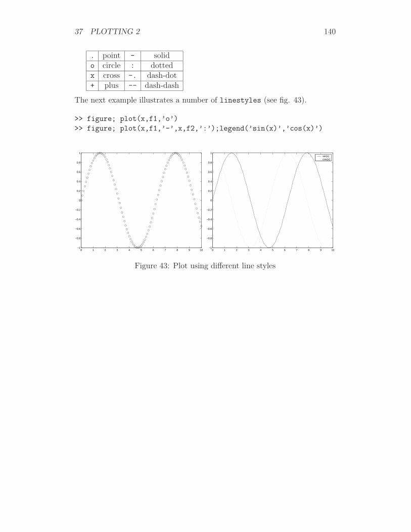
37 PLOTTING 2 140
. point - solido circle : dottedx cross -. dash-dot+ plus -- dash-dash
The next example illustrates a number of linestyles (see fig. 43).
>> figure; plot(x,f1,’o’)
>> figure; plot(x,f1,’-’,x,f2,’:’);legend(’sin(x)’,’cos(x)’)
0 1 2 3 4 5 6 7 8 9 10−1
−0.8
−0.6
−0.4
−0.2
0
0.2
0.4
0.6
0.8
1
0 1 2 3 4 5 6 7 8 9 10−1
−0.8
−0.6
−0.4
−0.2
0
0.2
0.4
0.6
0.8
1sin(x)cos(x)
Figure 43: Plot using different line styles
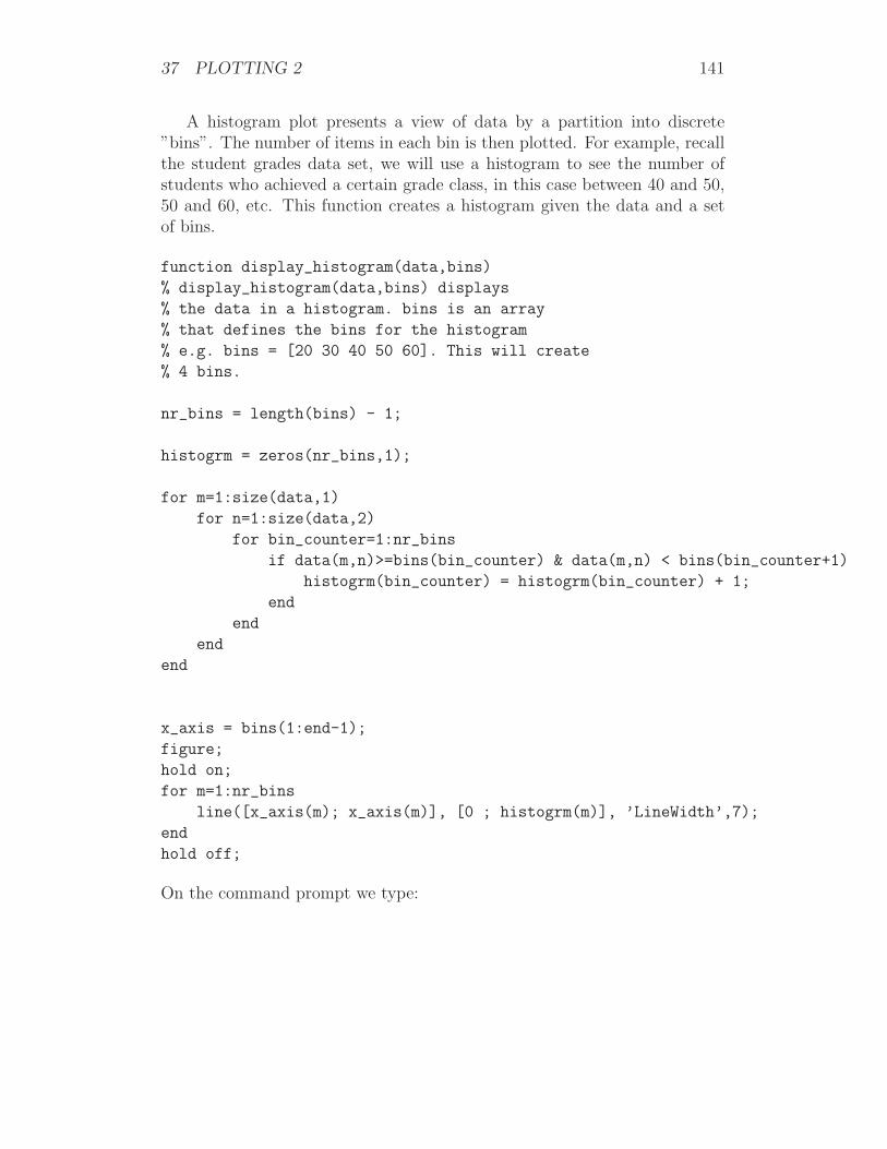
37 PLOTTING 2 141
A histogram plot presents a view of data by a partition into discrete”bins”. The number of items in each bin is then plotted. For example, recallthe student grades data set, we will use a histogram to see the number ofstudents who achieved a certain grade class, in this case between 40 and 50,50 and 60, etc. This function creates a histogram given the data and a setof bins.
function display_histogram(data,bins)
% display_histogram(data,bins) displays
% the data in a histogram. bins is an array
% that defines the bins for the histogram
% e.g. bins = [20 30 40 50 60]. This will create
% 4 bins.
nr_bins = length(bins) - 1;
histogrm = zeros(nr_bins,1);
for m=1:size(data,1)
for n=1:size(data,2)
for bin_counter=1:nr_bins
if data(m,n)>=bins(bin_counter) & data(m,n) < bins(bin_counter+1)
histogrm(bin_counter) = histogrm(bin_counter) + 1;
end
end
end
end
x_axis = bins(1:end-1);
figure;
hold on;
for m=1:nr_bins
line([x_axis(m); x_axis(m)], [0 ; histogrm(m)], ’LineWidth’,7);
end
hold off;
On the command prompt we type:

37 PLOTTING 2 142
>> display_histogram(data,[40:10:100])
40 45 50 55 60 65 70 75 80 85 900
5
10
15
20
25
30
Figure 44: Histogram plot
This will create fig. 44. To make the plot clearer we have drawn horizontallines using line(X,Y), where X and Y are vectors holding the starting andending point in x and y. After X,Y we can define any of the style propertiesof this line. In this particular example we have used ’LineWidth’, whichcan also be used in the plot function. ’LineWidth’ is followed by a scalardefining the width of the line.
To create 3D plots we can use meshgrid, which generates X and Y ma-trices for the coordinates.
>> dualgauss
= inline(’exp(-(x.^2+y.^2))+0.66 .*exp(-3*((x-3).^2+(y+2.5).^2))’,’x’,’y’)
dualgauss =
Inline function:
dualgauss(x,y) = exp(-(x.^2+y.^2))+0.66 .*exp(-3*((x-3).^2+(y+2.5).^2))
>> [X Y] = meshgrid(linspace(-4,4,30),linspace(-4,4,30));
>> Z = dualgauss(X,Y);
>> figure;meshc(X,Y,Z);
>> figure;surfc(X,Y,Z);
>> figure;contour(X,Y,Z,15);
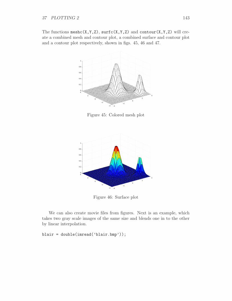
37 PLOTTING 2 143
The functions meshc(X,Y,Z), surfc(X,Y,Z) and contour(X,Y,Z) will cre-ate a combined mesh and contour plot, a combined surface and contour plotand a contour plot respectively, shown in figs. 45, 46 and 47.
−4
−2
0
2
4
−4
−2
0
2
40
0.2
0.4
0.6
0.8
1
Figure 45: Colored mesh plot
−4
−2
0
2
4
−4
−2
0
2
40
0.2
0.4
0.6
0.8
1
Figure 46: Surface plot
We can also create movie files from figures. Next is an example, whichtakes two gray scale images of the same size and blends one in to the otherby linear interpolation.
blair = double(imread(’blair.bmp’));
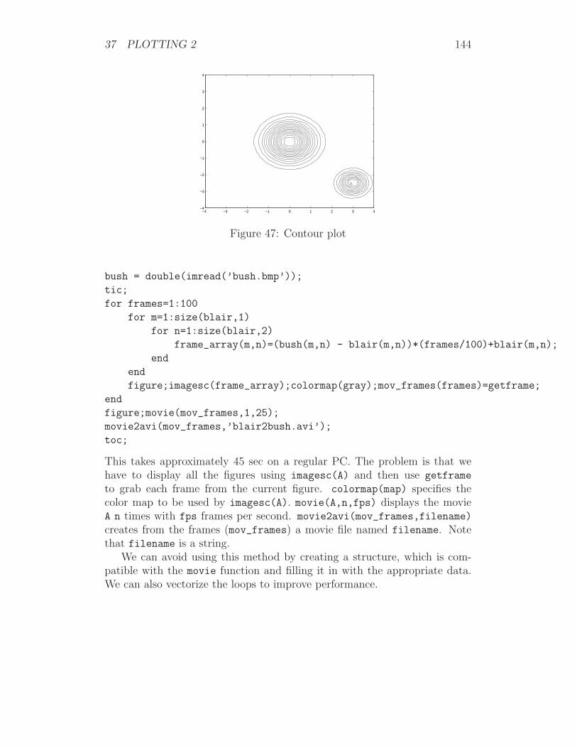
37 PLOTTING 2 144
−4 −3 −2 −1 0 1 2 3 4−4
−3
−2
−1
0
1
2
3
4
Figure 47: Contour plot
bush = double(imread(’bush.bmp’));
tic;
for frames=1:100
for m=1:size(blair,1)
for n=1:size(blair,2)
frame_array(m,n)=(bush(m,n) - blair(m,n))*(frames/100)+blair(m,n);
end
end
figure;imagesc(frame_array);colormap(gray);mov_frames(frames)=getframe;
end
figure;movie(mov_frames,1,25);
movie2avi(mov_frames,’blair2bush.avi’);
toc;
This takes approximately 45 sec on a regular PC. The problem is that wehave to display all the figures using imagesc(A) and then use getframe
to grab each frame from the current figure. colormap(map) specifies thecolor map to be used by imagesc(A). movie(A,n,fps) displays the movieA n times with fps frames per second. movie2avi(mov_frames,filename)
creates from the frames (mov_frames) a movie file named filename. Notethat filename is a string.
We can avoid using this method by creating a structure, which is com-patible with the movie function and filling it in with the appropriate data.We can also vectorize the loops to improve performance.
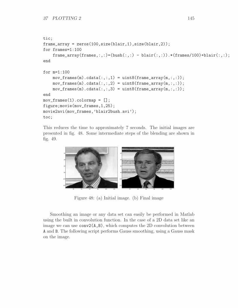
37 PLOTTING 2 145
tic;
frame_array = zeros(100,size(blair,1),size(blair,2));
for frames=1:100
frame_array(frames,:,:)=(bush(:,:) - blair(:,:)).*(frames/100)+blair(:,:);
end
for m=1:100
mov_frames(m).cdata(:,:,1) = uint8(frame_array(m,:,:));
mov_frames(m).cdata(:,:,2) = uint8(frame_array(m,:,:));
mov_frames(m).cdata(:,:,3) = uint8(frame_array(m,:,:));
end
mov_frames(1).colormap = [];
figure;movie(mov_frames,1,25);
movie2avi(mov_frames,’blair2bush.avi’);
toc;
This reduces the time to approximately 7 seconds. The initial images arepresented in fig. 48. Some intermediate steps of the blending are shown infig. 49.
20 40 60 80 100 120
20
40
60
80
100
120
20 40 60 80 100 120
20
40
60
80
100
120
Figure 48: (a) Initial image. (b) Final image
Smoothing an image or any data set can easily be performed in Matlabusing the built in convolution function. In the case of a 2D data set like animage we can use conv2(A,B), which computes the 2D convolution betweenA and B. The following script performs Gauss smoothing, using a Gauss maskon the image.
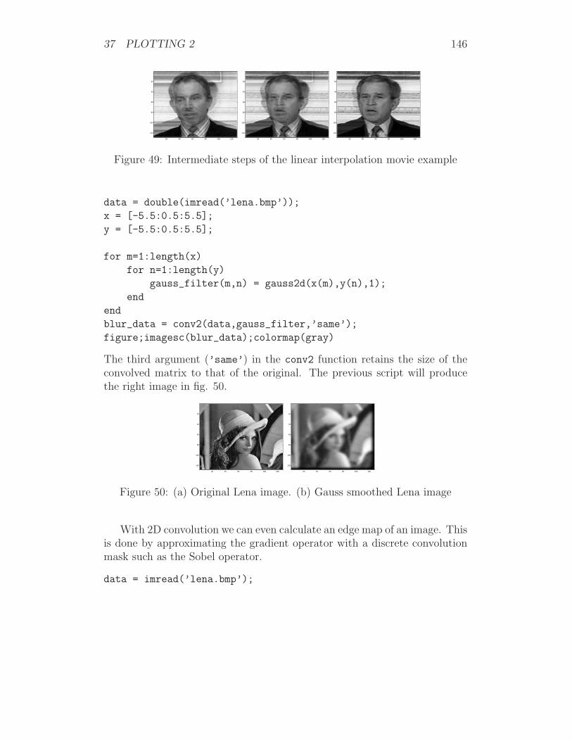
37 PLOTTING 2 146
20 40 60 80 100 120
20
40
60
80
100
120
20 40 60 80 100 120
20
40
60
80
100
120
20 40 60 80 100 120
20
40
60
80
100
120
Figure 49: Intermediate steps of the linear interpolation movie example
data = double(imread(’lena.bmp’));
x = [-5.5:0.5:5.5];
y = [-5.5:0.5:5.5];
for m=1:length(x)
for n=1:length(y)
gauss_filter(m,n) = gauss2d(x(m),y(n),1);
end
end
blur_data = conv2(data,gauss_filter,’same’);
figure;imagesc(blur_data);colormap(gray)
The third argument (’same’) in the conv2 function retains the size of theconvolved matrix to that of the original. The previous script will producethe right image in fig. 50.
20 40 60 80 100 120
20
40
60
80
100
120
20 40 60 80 100 120
20
40
60
80
100
120
Figure 50: (a) Original Lena image. (b) Gauss smoothed Lena image
With 2D convolution we can even calculate an edge map of an image. Thisis done by approximating the gradient operator with a discrete convolutionmask such as the Sobel operator.
data = imread(’lena.bmp’);
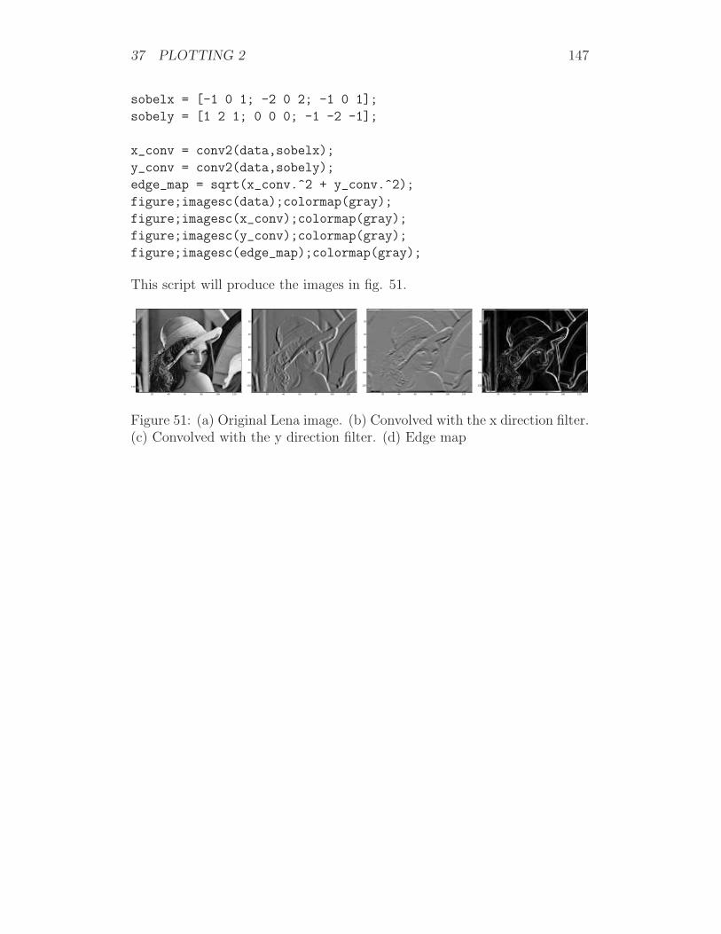
37 PLOTTING 2 147
sobelx = [-1 0 1; -2 0 2; -1 0 1];
sobely = [1 2 1; 0 0 0; -1 -2 -1];
x_conv = conv2(data,sobelx);
y_conv = conv2(data,sobely);
edge_map = sqrt(x_conv.^2 + y_conv.^2);
figure;imagesc(data);colormap(gray);
figure;imagesc(x_conv);colormap(gray);
figure;imagesc(y_conv);colormap(gray);
figure;imagesc(edge_map);colormap(gray);
This script will produce the images in fig. 51.
20 40 60 80 100 120
20
40
60
80
100
120
20 40 60 80 100 120
20
40
60
80
100
120
20 40 60 80 100 120
20
40
60
80
100
120
20 40 60 80 100 120
20
40
60
80
100
120
Figure 51: (a) Original Lena image. (b) Convolved with the x direction filter.(c) Convolved with the y direction filter. (d) Edge map

38 SUMMARY TABLE OF FUNCTIONS 148
38 Summary table of functions
Function p. Meaningprofile on/off 122 Turn profiler on/offprofile report 122 Generate profiler reportprofile resume 122 Resume profiler
tic - toc 122 Timersparse(a,b) 125 Create an a x b sparse matrixspeye(a) 127 Create an a x a sparse identity matrix
spfun(function,A) 127 Apply function to sparse matrixnnz(A) 127 Number of non-zero elements of Afull(A) 127 Convert sparse matrix to full
unique(A) 128 Find unique elements of a vector Aunion(A,B) 128 Set union of two vectors
intersect(A,B) 128 Set intersection of two vectorsismember(A,B) 128 Detects members of a setsetdiff(A,B) 128 Set difference of two vectors
global 130 Create global variablepersistent 130 Create persistent variable
inline(expr_string,arg1,...) 132 Create inline functionfigure 137 New figure window
figure(n) 137 Select figure window ntitle(string) 137 Give a title to the figure windowgtext(string) 137 Add text with the mouselegend(string) 137 Add a legendgrid on/off 137 Turn grid on/off
subplot(m,n,p) 137 Create multiple plotshold on/off 137 Hold the current graph in the figureline(X,Y) 142 Draw a line in a figure
meshc(X,Y,Z) 143 Create a colored mesh plotsurfc(X,Y,Z) 143 Create a colored surface plot
contour(X,Y,Z) 143 Create a contour plotimagesc(A) 144 Scale and display an image
colormap(map) 144 Specifies the color map to used by imagesc(A)
getframe 144 Grab a frame from the current figuremovie(A,n,fps) 144 Play movie A n times with fps frames per second
movie2avi(A,filename) 144 Create a movie fileconv2(A,B) 145 2D convolution between A and B
39 LAB EXERCISES 3 149
39 Lab exercises 3
Programming exercises 1
A. Given the 2D Gauss function z = e−x2+y
2
2σ2
.
1. Write a function that accepts three arguments, an array holding xvalues, an array holding y values and sigma, calculates the 2D Gaussfunction given above and returns the z values.
2. Write a script which uses for loops to calculate the 2D Gauss functionfor an array of x and y values.
3. Calculate the function for x = -2.5:0.01:2.5, y = -2.5:0.01:2.5
and sigma = 1. Use the profiler to find out how long it takes tocalculate this.
4. Use the tic-toc commands to time your function.
5. Use array preallocation and vectorize the loop. You might find themeshgrid command useful. Check how long it takes to calculate thisfunction and compare it with the previous non-optimized version.
6. Extend this function using varargin to accept two or three arguments.If only two arguments are entered then sigma will be equal to 1.
7. Write a function that makes use of persistent to count how many zvalues are above 0.5. You might find useful the counter example fromthe lecture notes.
B. Given the x,y values from the previous exercise.
1. Calculate the 2D Gauss function for sigma equals to 0.5, 1, 1.5, 2, 3, 4.
2. Using the subplot and the meshc command plot in one figure all sixgraphs.
C. Two sets are equal if all of their elements correspond regardless of theorder. Keep in mind that multiplicity of elements in a set is ignored.
1. Write a function that determines whether two sets are equal using theset functions.

39 LAB EXERCISES 3 150
2. Using varargin extend this function for any number of sets.
D. Given the display_histogram function in the lecture notes.
1. Modify the function to display the histogram horizontally as in fig. 52.
0 5 10 15 20 25 3040
45
50
55
60
65
70
75
80
85
90
Figure 52: Horizontal histogram
2. Extend the function using varargin to be able to accept an additionalargument LineWidth to define a new width for the line command.
D. Given two gray scale images of the same sizes.
1. Create a movie that starts from one image and blends it to the otherimage by linear interpolation.
2. Create a movie that starts from one image and moves it to the right,while at the same time inserting the right part of the other image onthe empty space on the left. The effect should a scrolling marqueebetween two images.
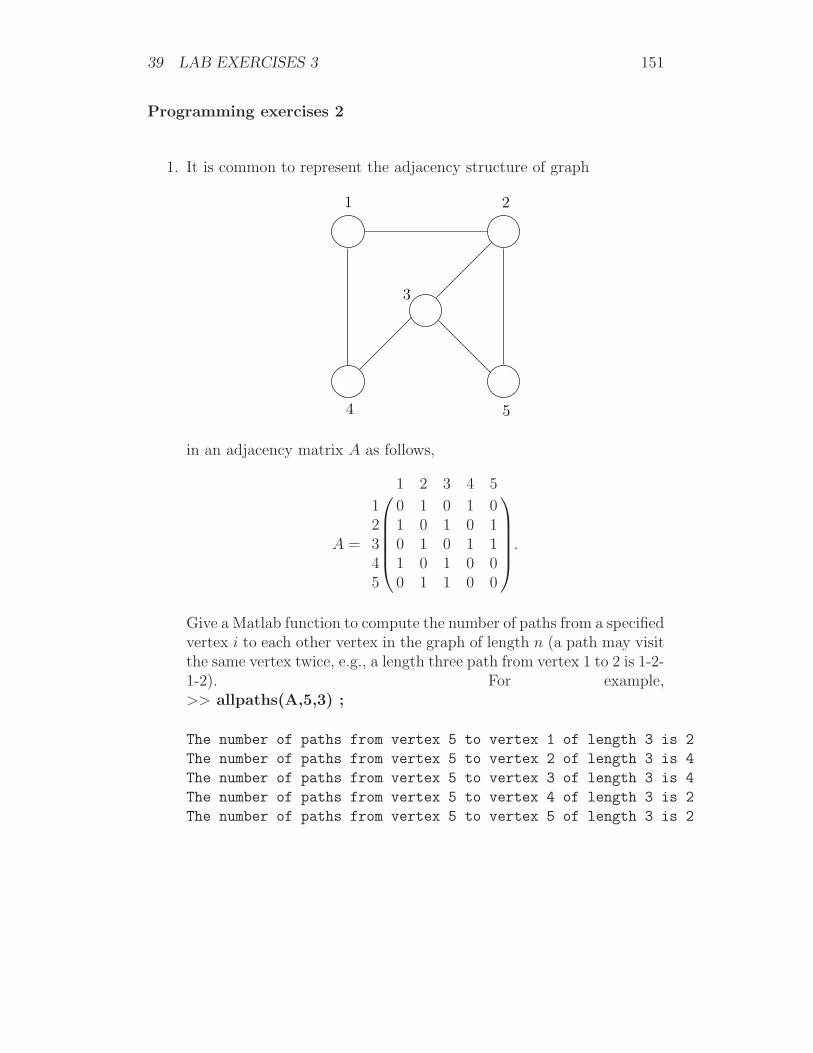
39 LAB EXERCISES 3 151
Programming exercises 2
1. It is common to represent the adjacency structure of graph
1 2
3
4 5
in an adjacency matrix A as follows,
A =
1 2 3 4 5
1 0 1 0 1 02 1 0 1 0 13 0 1 0 1 14 1 0 1 0 05 0 1 1 0 0
.
Give a Matlab function to compute the number of paths from a specifiedvertex i to each other vertex in the graph of length n (a path may visitthe same vertex twice, e.g., a length three path from vertex 1 to 2 is 1-2-1-2). For example,>> allpaths(A,5,3) ;
The number of paths from vertex 5 to vertex 1 of length 3 is 2
The number of paths from vertex 5 to vertex 2 of length 3 is 4
The number of paths from vertex 5 to vertex 3 of length 3 is 4
The number of paths from vertex 5 to vertex 4 of length 3 is 2
The number of paths from vertex 5 to vertex 5 of length 3 is 2

39 LAB EXERCISES 3 152
Hint: the algorithm to compute all paths of length n between all verticesmay be expressed in under 10 characters.
2. In many machine learning algorithms it is important to generate a ran-dom permutation of a dataset. Matlab provides a function randperm(n)that returns a random permutation of the numbers 1 . . . n in an arraysuch that each of the n! permutations have equal probability (with theusual proviso of pseudo-randomness of the base random number gen-erator).
Write a function myrandperm(n) with functionally similar behavior alsoassuring that each of the n! possible permutations have equal proba-bility of being generated. The best marks will be given for a functionwhose running time is linear in n.
3. In this problem you will implement some simple drawing functions.The top-level function developed will be able to plot a figure consistingof lines, triangles, rectangles, and circles. The function should take oneargument, the figure filename. In the file each line contains a singlecharacter denoting the element to be drawn and the data needed tospecify the element, i.e.,
L x1 y1 x2 y2
T x1 y1 x2 y2 x3 y3
R x1 y1 x2 y2 % these are the opposite corners of the rectangle
C x1 y1 radius
Demonstrate your function with the following file afig.txt which mayalso be found from the class web page.
C 5 17 0.5
R 6 0 8 1
L 1 9 1 7
C 4 15 4
T 3.5 15 4.5 15 4 16
L 4 4 4 11
L 4 4 6 1
C 3 17 0.5
R 0 0 2 1

39 LAB EXERCISES 3 153
L 1 2 4 4
L 1 19 7 19
T 3 19 4 22 5 19
R 3 12.5 5 13.5