CS 189Spring 2020

Introduction toMachine Learning Final Exam

• The exam is open book, open notes, and open web. However, you may not consult or communicate with other people(besides your exam proctors).

• You will submit your answers to the multiple-choice questions through Gradescope via the assignment “Final Exam– Multiple Choice”; please do not submit your multiple-choice answers on paper. By contrast, you will submit youranswers to the written questions by writing them on paper by hand, scanning them, and submitting them through Grade-scope via the assignment “Final Exam – Writeup.”

• Please write your name at the top of each page of your written answers. (You may do this before the exam.)

• You have 180 minutes to complete the midterm exam (3:00–6:00 PM). (If you are in the DSP program and have anallowance of 150% or 200% time, that comes to 270 minutes or 360 minutes, respectively.)

• When the exam ends (6:00 PM), stop writing. You must submit your multiple-choice answers before 6:00 PM sharp.Late multiple-choice submissions will be penalized at a rate of 5 points per minute after 6:00 PM. (The multiple-choicequestions are worth 60 points total.)

• From 6:00 PM, you have 15 minutes to scan the written portion of your exam and turn it into Gradescope via theassignment “Final Exam – Writeup.” Most of you will use your cellphone and a third-party scanning app. If you have aphysical scanner, you may use that. Late written submissions will be penalized at a rate of 5 points per minute after 6:15PM.

• Mark your answers to multiple-choice questions directly into Gradescope. Write your answers to written questions onblank paper. Clearly label all written questions and all subparts of each written question. Show your work inwritten questions.

• Following the exam, you must use Gradescope’s page selection mechanism to mark which questions are on which pagesof your exam (as you do for the homeworks).

• The total number of points is 150. There are 16 multiple choice questions worth 4 points each, and six written questionsworth 86 points total.

• For multiple answer questions, fill in the bubbles for ALL correct choices: there may be more than one correct choice,but there is always at least one correct choice. NO partial credit on multiple answer questions: the set of all correctanswers must be checked.

First name

Last name

SID

1

Q1. [64 pts] Multiple AnswerFill in the bubbles for ALL correct choices: there may be more than one correct choice, but there is always at least one correctchoice. NO partial credit: the set of all correct answers must be checked.

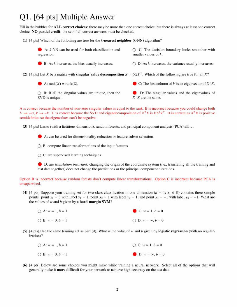
(1) [4 pts] Which of the following are true for the k-nearest neighbor (k-NN) algorithm?

A: k-NN can be used for both classification andregression.

B: As k increases, the bias usually increases.

© C: The decision boundary looks smoother withsmaller values of k.

© D: As k increases, the variance usually increases.

(2) [4 pts] Let X be a matrix with singular value decomposition X = UΣV>. Which of the following are true for all X?

A: rank(X) = rank(Σ).

© B: If all the singular values are unique, then theSVD is unique.

C: The first column of V is an eigenvector of X>X.

D: The singular values and the eigenvalues ofX>X are the same.

A is correct because the number of non-zero singular values is equal to the rank. B is incorrect because you could change bothU → −U,V → −V . C is correct because the SVD and eigendecomposition of X>X is VΣ2V>. D is correct as X>X is positivesemidefinite, so the eigenvalues can’t be negative.

(3) [4 pts] Lasso (with a fictitious dimension), random forests, and principal component analysis (PCA) all . . .

A: can be used for dimensionality reduction or feature subset selection

© B: compute linear transformations of the input features

© C: are supervised learning techniques

D: are translation invariant: changing the origin of the coordinate system (i.e., translating all the training andtest data together) does not change the predictions or the principal component directions

Option B is incorrect because random forests don’t compute linear transformations. Option C is incorrect because PCA isunsupervised.

(4) [4 pts] Suppose your training set for two-class classification in one dimension (d = 1; xi ∈ R) contains three samplepoints: point x1 = 3 with label y1 = 1, point x2 = 1 with label y2 = 1, and point x3 = −1 with label y3 = −1. What arethe values of w and b given by a hard-margin SVM?

© A: w = 1, b = 1

© B: w = 0, b = 1

C: w = 1, b = 0

© D: w = ∞, b = 0

(5) [4 pts] Use the same training set as part (d). What is the value of w and b given by logistic regression (with no regular-ization)?

© A: w = 1, b = 1

© B: w = 0, b = 1

© C: w = 1, b = 0

D: w = ∞, b = 0

(6) [4 pts] Below are some choices you might make while training a neural network. Select all of the options that willgenerally make it more difficult for your network to achieve high accuracy on the test data.

2

A: Initializing the weights to all zeros

B: Normalizing the training data but leaving thetest data unchanged

© C: Using momentum

© D: Reshuffling the training data at the beginningof each epoch

A) Initializing weights with zeros makes it impossible to learn. B) Mean and standard deviation should be computed on thetraining set and then used to standardize the validation and test sets, so that the distributions are matched for each set. C) Thisdescribes momentum and will generally help training. D) This is best practice.

3

(7) [4 pts] To the left of each graph below is a number. Select the choices for which the number is the multiplicity of theeigenvalue zero in the Laplacian matrix of the graph.

© A: 1

B: 1

© C: 2

© D: 4

The multiplicity is equal to the number of connected components in the graph.

(8) [4 pts] Given the spectral graph clustering optimization problemFind y that minimizes y>Lysubject to y>y = n

and 1>y = 0,which of the following optimization problems produce a vector y that leads to the same sweep cut as the optimizationproblem above? M is a diagonal mass matrix with different masses on the diagonal.

A:Minimize y>Lysubject to y>y = 1

and 1>y = 0

© B:Minimize y>Lysubject to ∀i, yi = 1 or yi = −1

and 1>y = 0

C: Minimize y>Ly/(y>y)subject to 1>y = 0

© D:Minimize y>Lysubject to y>My = 1

and 1>My = 0

(9) [4 pts] Which of the following methods will cluster the data in panel (a) of the figure below into the two clusters (redcircle and blue horizontal line) shown in panel (b)? Every dot in the circle and the line is a data point. In all the optionsthat involve hierarchical clustering, the algorithm is run until we obtain two clusters.

(a) Unclustered

(b) Desired clustering

© A: Hierarchical agglomerative clustering withEuclidean distance and complete linkage

B: Hierarchical agglomerative clustering withEuclidean distance and single linkage

4

© C: Hierarchical agglomerative clustering withEuclidean distance and centroid linkage

© D: k-means clustering with k = 2

Single linkage uses the minimum distance between two clusters as a metric for merging clusters. Since the two clusters aredensely packed with points and the minimum distance between the two clusters is greater than the within-cluster distancesbetween points, single linkage doesn’t link the circle to the line until the very end.

The other three methods will all join some of the points at the left end of the line with the circle, before they are joined with theright end of the line.

5

(10) [4 pts] Which of the following statement(s) about kernels are true?

A: The dimension of the lifted feature vectors Φ(·), whose inner products the kernel function computes, can beinfinite.

© B: For any desired lifting Φ(x), we can design a kernel function k(x, z) that will evaluate Φ(x)>Φ(z) more quicklythan explicitly computing Φ(x) and Φ(z).

C: The kernel trick, when it is applicable, speeds up a learning algorithm if the number of sample points issubstantially less than the dimension of the (lifted) feature space.

D: If the raw feature vectors x, y are of dimension 2, then k(x, y) = x21y2

1 + x22y2

2 is a valid kernel.

A is correct; consider the Gaussian kernel from lecture. B is wrong; most liftings don’t lead to super-fast kernels. Just somespecial ones do. C is correct, straight from lecture. Though in this case, the dual algorithm is faster than the primal whetheryou use a fancy kernel or not. D is correct because k(x, y) is inner product of Φ(x) = [x2

1 x22]> and Φ(y) = [y2

1 y22]>.

(11) [4 pts] We want to use a decision tree to classify the training points depicted. Which of the following decision treeclassifiers is capable of giving 100% accuracy on the training data with four splits or fewer?

© A: A standard decision tree with axis-aligned splits

© B: Using PCA to reduce the training data to onedimension, then applying a standard decision tree

C: A decision tree with multivariate linear splits

D: Appending a new feature |x1| + |x2| to eachsample point x, then applying a standard decision tree

A standard decision tree will need (substantially) more than four splits. PCA to 1D will make it even harder. However,four non-axis-aligned multivariate linear splits suffice to cut the diamond out of the center. Finally, adding the L1 normfeature lets us perfectly classify the data with a single split that cuts off the top of the pyramid.

(12) [4 pts] Which of the following are true about principal components analysis (PCA)?

© A: The principal components are eigenvectors ofthe centered data matrix.

B: The principal components are right singularvectors of the centered data matrix.

C: The principal components are eigenvectors ofthe sample covariance matrix.

D: The principal components are right singularvectors of the sample covariance matrix.

The first three follow directly from definitions. The last is because the covariance matrix is symmetric, so the singular vectorsare the eigenvectors.

6

(13) [4 pts] Suppose we are doing ordinary least-squares linear regression with a fictitious dimension. Which of thefollowing changes can never make the cost function’s value on the training data smaller?

A: Discard the fictitious dimension (i.e., don’t append a 1 to every sample point).

© B: Append quadratic features to each sample point.

C: Project the sample points onto a lower-dimensional subspace with PCA (without changing the labels) andperform regression on the projected points.

D: Center the design matrix (so each feature has mean zero).

A: Correct. Discarding the fictitious dimension forces the linear regression function to be zero at the origin, which may increasethe cost function but can never decrease it.

B: Incorrect. Added quadratic features often help to fit the data better.

C: Correct. Regular OLS is at least as expressive. Projecting the points may incrase the cost function but can never decreaseit. Centering features doesn’t matter so WLOG assume X has centered features. If the full SVD is X = UΣV>, then projectingonto a k-dimensional subspace gives Xk = UΣkV>. If wk is a solution for the PCA-projected OLS, we can take w = Vz where zis the first k elements of V>wk with the rest zero, and get Xkwk = Xw.

D: Correct. Since we’re using a fictitious dimension, translating the points does not affect the cost of the optimal regressionfunction (which translates with the points).

7

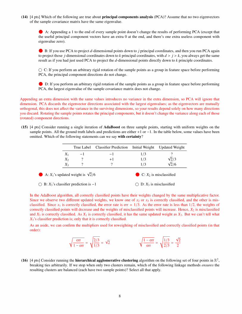
(14) [4 pts] Which of the following are true about principal components analysis (PCA)? Assume that no two eigenvectorsof the sample covariance matrix have the same eigenvalue.

A: Appending a 1 to the end of every sample point doesn’t change the results of performing PCA (except thatthe useful principal component vectors have an extra 0 at the end, and there’s one extra useless component witheigenvalue zero).

B: If you use PCA to project d-dimensional points down to j principal coordinates, and then you run PCA againto project those j-dimensional coordinates down to k principal coordinates, with d > j > k, you always get the sameresult as if you had just used PCA to project the d-dimensional points directly down to k principle coordinates.

© C: If you perform an arbitrary rigid rotation of the sample points as a group in feature space before performingPCA, the principal component directions do not change.

D: If you perform an arbitrary rigid rotation of the sample points as a group in feature space before performingPCA, the largest eigenvalue of the sample covariance matrix does not change.

Appending an extra dimension with the same values introduces no variance in the extra dimension, so PCA will ignore thatdimension. PCA discards the eigenvector directions associated with the largest eigenvalues; as the eigenvectors are mutuallyorthogonal, this does not affect the variance in the surviving dimensions, so your results depend solely on how many directionsyou discard. Rotating the sample points rotates the principal components, but it doesn’t change the variance along each of those(rotated) component directions.

(15) [4 pts] Consider running a single iteration of AdaBoost on three sample points, starting with uniform weights on thesample points. All the ground truth labels and predictions are either +1 or −1. In the table below, some values have beenomitted. Which of the following statements can we say with certainty?

True Label Classifier Prediction Initial Weight Updated Weight

X1 −1 −1 1/3 ?X2 ? +1 1/3

√2/3

X3 ? ? 1/3√

2/6

A: X1’s updated weight is√

2/6

© B: X3’s classifier prediction is −1

C: X2 is misclassified

© D: X3 is misclassified

In the AdaBoost algorithm, all correctly classified points have their weights changed by the same multiplicative factor.Since we observe two different updated weights, we know one of x2 or x3 is correctly classified, and the other is mis-classified. Since x1 is correctly classified, the error rate is err = 1/3. As the error rate is less than 1/2, the weights ofcorrectly classified points will decrease and the weights of misclassified points will increase. Hence, X2 is misclassifiedand X3 is correctly classified. As X1 is correctly classified, it has the same updated weight as X3. But we can’t tell whatX3’s classifier prediction is; only that it is correctly classified.

As an aside, we can confirm the multipliers used for reweighting of misclassified and correctly classified points (in thatorder): √

err1 − err

=

√2/31/3

=√

2

√1 − err

err=

√1/32/3

=

√2

2

(16) [4 pts] Consider running the hierarchical agglomerative clustering algorithm on the following set of four points in R2,breaking ties arbitrarily. If we stop when only two clusters remain, which of the following linkage methods ensures theresulting clusters are balanced (each have two sample points)? Select all that apply.

8

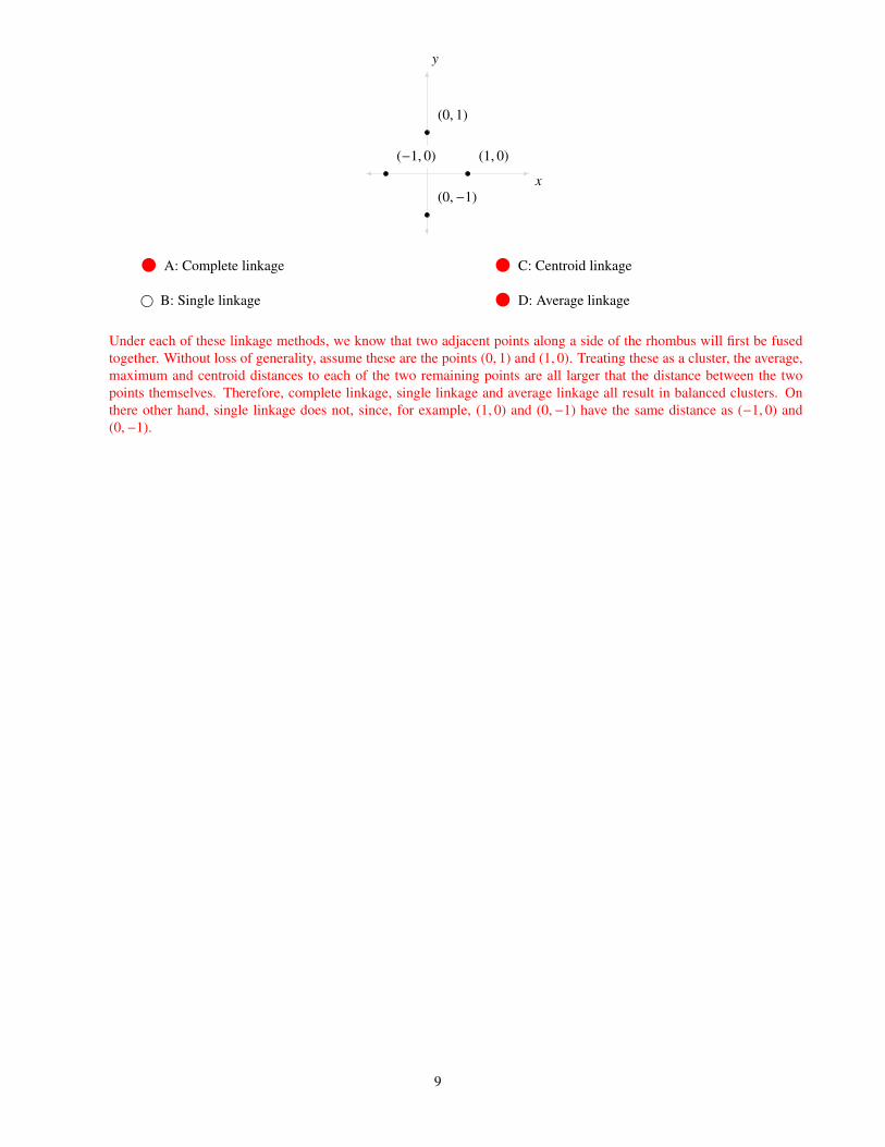
y

x

(0, 1)

(0,−1)

(1, 0)(−1, 0)

A: Complete linkage

© B: Single linkage

C: Centroid linkage

D: Average linkage

Under each of these linkage methods, we know that two adjacent points along a side of the rhombus will first be fusedtogether. Without loss of generality, assume these are the points (0, 1) and (1, 0). Treating these as a cluster, the average,maximum and centroid distances to each of the two remaining points are all larger that the distance between the twopoints themselves. Therefore, complete linkage, single linkage and average linkage all result in balanced clusters. Onthere other hand, single linkage does not, since, for example, (1, 0) and (0,−1) have the same distance as (−1, 0) and(0,−1).

9

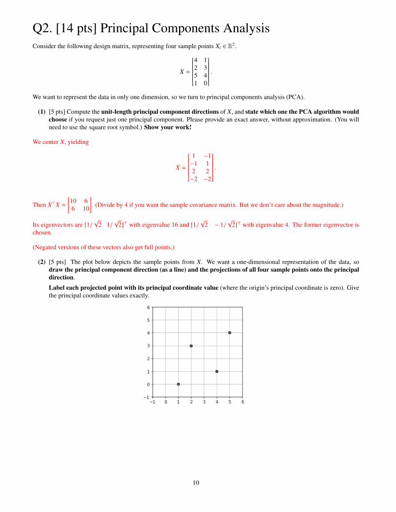
Q2. [14 pts] Principal Components AnalysisConsider the following design matrix, representing four sample points Xi ∈ R

2.

X =

4 12 35 41 0

.We want to represent the data in only one dimension, so we turn to principal components analysis (PCA).

(1) [5 pts] Compute the unit-length principal component directions of X, and state which one the PCA algorithm wouldchoose if you request just one principal component. Please provide an exact answer, without approximation. (You willneed to use the square root symbol.) Show your work!

We center X, yielding

X =

1 −1−1 12 2−2 −2

.

Then X>X =

[10 66 10

]. (Divide by 4 if you want the sample covariance matrix. But we don’t care about the magnitude.)

Its eigenvectors are [1/√

2 1/√

2]> with eigenvalue 16 and [1/√

2 − 1/√

2]> with eigenvalue 4. The former eigenvector ischosen.

(Negated versions of these vectors also get full points.)

(2) [5 pts] The plot below depicts the sample points from X. We want a one-dimensional representation of the data, sodraw the principal component direction (as a line) and the projections of all four sample points onto the principaldirection.

Label each projected point with its principal coordinate value (where the origin’s principal coordinate is zero). Givethe principal coordinate values exactly.

10

The principal coordinates are 1√

2, 5√

2, 5√

2, and 9

√2. (Alternatively, all of these could be negative, but they all have to have the

same sign.)

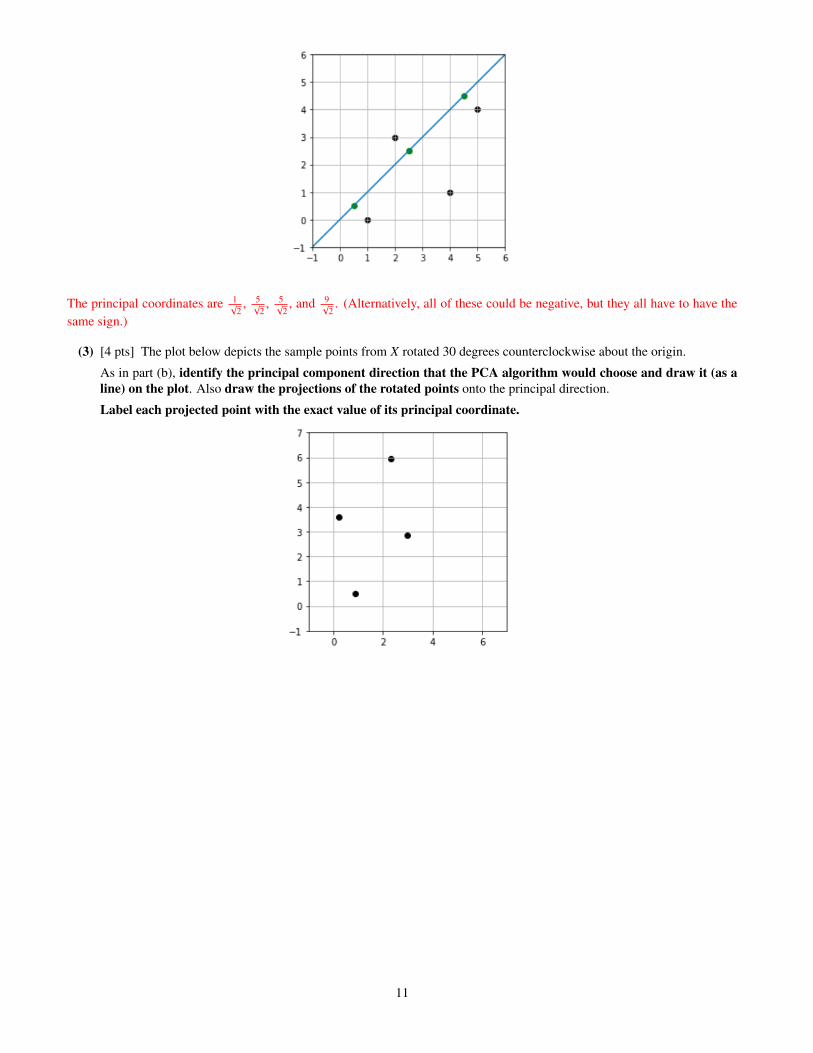
(3) [4 pts] The plot below depicts the sample points from X rotated 30 degrees counterclockwise about the origin.

As in part (b), identify the principal component direction that the PCA algorithm would choose and draw it (as aline) on the plot. Also draw the projections of the rotated points onto the principal direction.

Label each projected point with the exact value of its principal coordinate.

11

The line passes through the origin and is parallel to the two sample points that are farthest apart, so it’s easy to draw. Rotationhas not changed the principal coordinates: 1

√2, 5√

2, 5√

2, and 9

√2. (Again, these could all be negative.)

12

Q3. [14 pts] A Decision TreeIn this question we investigate whether students will pass or fail CS 189 based on whether or not they studied, cheated, andslept well before the exam. You are given the following data for five students. There are three features, “Studied,” “Slept,” and“Cheated.” The column “Result” shows the label we want to predict.

Studied Slept Cheated ResultStudent 1 Yes No No PassedStudent 2 Yes No Yes FailedStudent 3 No Yes No FailedStudent 4 Yes Yes Yes FailedStudent 5 Yes Yes No Passed

(1) [4 pts] What is the entropy H(Result) at the root node? (There is no need to compute the exact number; you may writeit as an arithmetic expression.)

H(Result) = −

(25

log225

+35

log235

).

(2) [5 pts] Draw the decision tree where every split maximizes the information gain. (An actual drawing, please; a writtendescription does not suffice.) Do not perform a split on a pure leaf or if the split will produce an empty child; otherwise,split. Explain (with numbers) why you chose the splits you chose.

A tree that first splits on “Cheated” and then “Studied.”

(3) [2 pts] Did the tree you built implicitly perform feature subset selection? Explain.

Yes, because it does not use the feature “Slept.”

(4) [3 pts] Suppose you have a sample of n students for some large n, with the same three features. Assuming that we use areasonably efficient algorithm to build the tree (as discussed in class), what is the worst-case running time to build thedecision tree? (Write your answer in the simplest asymptotic form possible.) Why?

We have 3 binary features, so the tree’s depth cannot exceed 3 and each sample point participates in at most four treenodes.Hence, it cannot take more than Θ(n) time to build the tree.

13

Q4. [20 pts] Spectral Graph Clustering

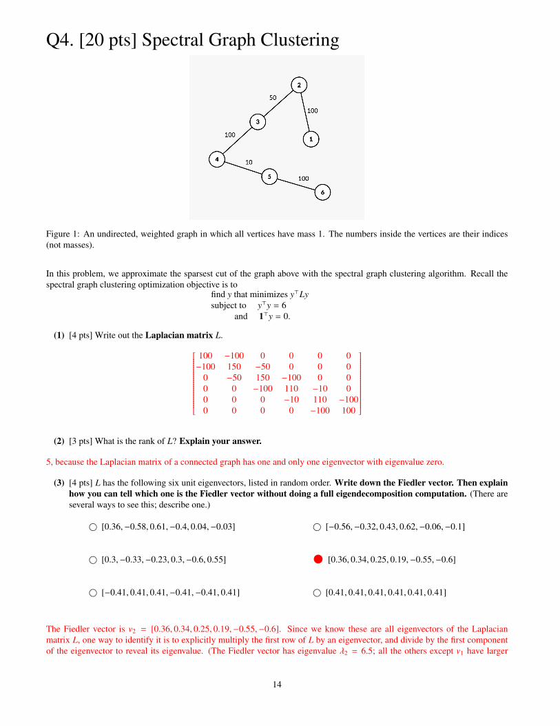
Figure 1: An undirected, weighted graph in which all vertices have mass 1. The numbers inside the vertices are their indices(not masses).

In this problem, we approximate the sparsest cut of the graph above with the spectral graph clustering algorithm. Recall thespectral graph clustering optimization objective is to

find y that minimizes y>Lysubject to y>y = 6

and 1>y = 0.

(1) [4 pts] Write out the Laplacian matrix L.

100 −100 0 0 0 0−100 150 −50 0 0 0

0 −50 150 −100 0 00 0 −100 110 −10 00 0 0 −10 110 −1000 0 0 0 −100 100

(2) [3 pts] What is the rank of L? Explain your answer.

5, because the Laplacian matrix of a connected graph has one and only one eigenvector with eigenvalue zero.

(3) [4 pts] L has the following six unit eigenvectors, listed in random order. Write down the Fiedler vector. Then explainhow you can tell which one is the Fiedler vector without doing a full eigendecomposition computation. (There areseveral ways to see this; describe one.)

© [0.36,−0.58, 0.61,−0.4, 0.04,−0.03]

© [0.3,−0.33,−0.23, 0.3,−0.6, 0.55]

© [−0.41, 0.41, 0.41,−0.41,−0.41, 0.41]

© [−0.56,−0.32, 0.43, 0.62,−0.06,−0.1]

[0.36, 0.34, 0.25, 0.19,−0.55,−0.6]

© [0.41, 0.41, 0.41, 0.41, 0.41, 0.41]

The Fiedler vector is v2 = [0.36, 0.34, 0.25, 0.19,−0.55,−0.6]. Since we know these are all eigenvectors of the Laplacianmatrix L, one way to identify it is to explicitly multiply the first row of L by an eigenvector, and divide by the first componentof the eigenvector to reveal its eigenvalue. (The Fiedler vector has eigenvalue λ2 = 6.5; all the others except v1 have larger

14

eigenvalues.) An easier way is to notice that only the Fiedler vector is monotonic in one direction (decreasing in this example).

(4) [5 pts] How does the sweep cut decide how to cut this graph into two clusters? (Explain in clear English sentences.) Forevery cut considered by the algorithm, write down the “score” it is assigned by the sweep cut algorithm. (You may usefractions; decimal numbers aren’t required.) Identify the chosen cut by writing down two sets of vertex indices.

The sweep cut sorts the values in the Fiedler vector, then decides which pair of consecutive vertices to cut between by explicitlycomputing the sparsity of each of the five possible cuts. The cut with the lowest sparsity wins.

From left to right in the Fiedler vector, the sparsity of each cut is 20, 508 = 6.25, 100

9 � 11.11, 108 = 1.25, and 20.

The clusters are {5, 6} and {4, 3, 1, 2}.

(Cut between the values 0.19 and −0.55.)

(5) [4 pts] Suppose we have computed the four eigenvectors v1, v2, v3, v4 corresponding to the four largest eigenvalues.(For simplicity, assume no two eigenvectors have the same eigenvalue.) We want to write a constrained optimizationproblem that identifies the eigenvector corresponding to the fifth-largest eigenvalue. Explain how to modify theoptimization problem at the beginning of this question so that the vector y it finds is the desired eigenvector. (You maychange the objective function and/or add constraints, but they must be mathematical, and you cannot write things like“subject to y being the eigenvector corresponding to the fifth-largest eigenvalue.”)

Add the following constraints: v>2 y = 0, v>3 y = 0, v>4 y = 0.

15

Q5. [12 pts] Hierarchical Spectral Graph Multi-ClusteringIn this problem, we shall consider the same graph as in the previous question, but we use multiple eigenvectors to perform3-cluster clustering with the algorithm of Ng, Jordan, and Weiss (as opposed to the 2-cluster clustering we performed in the lastquestion).

(1) [4 pts] Based on the six eigenvectors of L given in the previous question, write down the spectral vector (as defined inthe lecture notes) for each vertex 1, . . . , 6 in that order.

The matrix of spectral vectors is

0.41 0.36 −0.560.41 0.34 −0.320.41 0.25 0.430.41 0.19 0.620.41 −0.55 −0.060.41 −0.6 −0.1

.

(2) [8 pts] We shall now cluster the six raw, unnormalized spectral vectors obtained above using hierarchical agglomerativeclustering with the Euclidean distance metric and single linkage. In contrast to what was discussed in class, we are notnormalizing the six spectral vectors (because we don’t want you to work that hard). Draw the complete single linkagedendrogram on paper. The six integer points on the x-axis, 1, . . . , 6, should represent the vertices of the graph in theorder of their indices. The y-axis should indicate the linkage distances, as is standard for dendrograms. The numericaldistance at which each fusion happens should be clearly marked on your figure.

Points 5 and 6 merge first; the Euclidean distance between them is 0.06. Points 3 and 4 merge next; the Euclidean distancebetween them is 0.2. Points 1 and 2 merge next; the Euclidean distance between them is 0.24. The single linkage distancebetween {1, 2} and {3, 4} is 0.76. The single linkage distance between {1, 2} and {5, 6} is 0.93. That between {3, 4} and {5, 6} is0.94. Therefore, the fourth merger is between {1, 2} and {3, 4}. The clusters after the fourth merger are {1, 2, 3, 4} and {5, 6},matching what we obtained in the previous question. {1, 2, 3, 4} and {5, 6} merge at 0.93. The green dotted line indicates the2-cluster clustering. The red dotted line indicates the 3-cluster clustering. (Note tha students aren’t asked to specify those lines.)

0 1 2 3 4 5 6 70

0.2

0.4

0.6

0.8

1

1.2

16

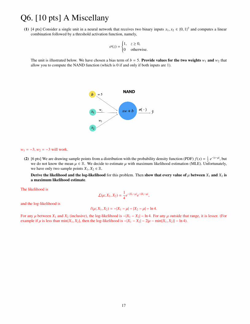
Q6. [10 pts] A Miscellany(1) [4 pts] Consider a single unit in a neural network that receives two binary inputs x1, x2 ∈ {0, 1}2 and computes a linear

combination followed by a threshold activation function, namely,

σ(z) =

1, z ≥ 0,0 otherwise.

The unit is illustrated below. We have chosen a bias term of b = 5. Provide values for the two weights w1 and w2 thatallow you to compute the NAND function (which is 0 if and only if both inputs are 1).

w1 = −3, w2 = −3 will work.

(2) [6 pts] We are drawing sample points from a distribution with the probability density function (PDF) f (x) = 12 e−|x−µ|, but

we do not know the mean µ ∈ R. We decide to estimate µ with maximum likelihood estimation (MLE). Unfortunately,we have only two sample points X1, X2 ∈ R.

Derive the likelihood and the log-likelihood for this problem. Then show that every value of µ between X1 and X2 isa maximum likelihood estimate.

The likelihood isL(µ; X1, X2) =

14

e−|X1−µ|e−|X2−µ|,

and the log-likelihood is`(µ; X1, X2) = −|X1 − µ| − |X2 − µ| − ln 4.

For any µ between X1 and X2 (inclusive), the log-likelihood is −|X1 − X2| − ln 4. For any µ outside that range, it is lesser. (Forexample if µ is less than min{X1, X2}, then the log-likelihood is −|X1 − X2| − 2|µ −min{X1, X2}| − ln 4).

17

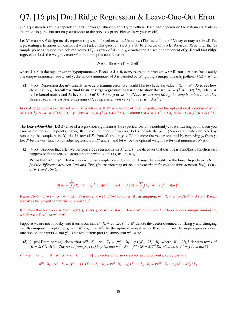
Q7. [16 pts] Dual Ridge Regression & Leave-One-Out Error[This question has four independent parts. If you get stuck on one, try the others. Each part depends on the statements made inthe previous parts, but not on your answer to the previous parts. Please show your work!]

Let X be an n × d design matrix representing n sample points with d features. (The last column of X may or may not be all 1’s,representing a fictitious dimension; it won’t affect this question.) Let y ∈ Rn be a vector of labels. As usual, Xi denotes the ithsample point expressed as a column vector (X>i is row i of X) and yi denotes the ith scalar component of y. Recall that ridgeregression finds the weight vector w∗ minimizing the cost function

J(w) = ‖Xw − y‖2 + λ‖w‖2

where λ > 0 is the regularization hyperparameter. Because λ > 0, every regression problem we will consider here has exactlyone unique minimizer. For X and y, the unique minimizer of J is denoted by w∗, giving a unique linear hypothesis h(z) = w∗ · z.

(1) [4 pts] Regression doesn’t usually have zero training error; we would like to check the value h(Xi) = w∗ · Xi to see howclose it is to yi. Recall the dual form of ridge regression and use it to show that w∗ · Xi = y>(K + λI)−1Ki, where Kis the kernel matrix and Ki is column i of K. Show your work. (Note: we are not lifting the sample points to anotherfeature space; we are just doing dual ridge regression with kernel matrix K = XX>.)

In dual ridge regression, we set w = X>a where a ∈ Rn is a vector of dual weights, and the optimal dual solution is a∗ =

(K +λI)−1y, so w∗ = X>(K +λI)−1y. Thus w∗ ·Xi = y>(K +λI)−1XXi. Column i of K = XX> is XXi, so w∗ ·Xi = y>(K +λI)−1Ki.

The Leave-One-Out (LOO) error of a regression algorithm is the expected loss on a randomly chosen training point when youtrain on the other n − 1 points, leaving the chosen point out of training. Let Xi denote the (n − 1) × d design matrix obtained byremoving the sample point Xi (the ith row of X) from X, and let yi ∈ Rn−1 denote the vector obtained by removing yi from y.Let Ji be the cost function of ridge regression on Xi and yi, and let wi be the optimal weight vector that minimizes Ji(w).

(2) [4 pts] Suppose that after we perform ridge regression on Xi and yi, we discover that our linear hypothesis function justhappens to fit the left-out sample point perfectly; that is, wi · Xi = yi.

Prove that w∗ = wi. That is, removing the sample point Xi did not change the weights or the linear hypothesis. (Hint:find the difference between J(w) and Ji(w) (for an arbitrary w), then reason about the relationships between J(w), Ji(w),Ji(wi), and J(wi).)

J(w) =

n∑j=1

(X j · w − y j)2 + λ‖w‖2 and Ji(w) =∑j,i

(X j · w − y j)2 + λ‖w‖2.

Hence J(w) − Ji(w) = (Xi · w − yi)2. Therefore, J(w) ≥ Ji(w) for all w. By assumption, wi · Xi = yi, so J(wi) = Ji(wi). Recallthat wi is the weight vector that minimizes Ji.

It follows that for every w ∈ Rd, J(w) ≥ Ji(w) ≥ Ji(wi) = J(wi). Hence wi minimizes J. J has only one unique minimizer,which we call w∗, so w∗ = wi.

Suppose we are not so lucky, and it turns out that wi · Xi , yi. Let y(i) ∈ Rn denote the vector obtained by taking y and changingthe ith component, replacing yi with wi · Xi. Let w(i) be the optimal weight vector that minimizes the ridge regression costfunction on the inputs X and y(i). Our result from part (b) shows that w(i) = wi.

(3) [4 pts] From part (a), show that w(i) · Xi − w∗ · Xi = (w(i) · Xi − yi) (K + λI)−1i Ki, where (K + λI)−1

i denotes row i of(K + λI)−1. (Hint: The result from part (a) implies that w(i) · Xi = y(i) · (K + λI)−1Ki. What does y(i) − y look like?)

y(i) − y = [0 . . . 0 wi · Xi − yi 0 . . . 0]>, a vector of all zeros except in component i, so by part (a),

w(i) · Xi − w∗ · Xi = (y(i) − y)>(K + λI)−1Ki = (wi · Xi − yi) (K + λI)−1i Ki = (w(i) · Xi − yi) (K + λI)−1

i Ki.

18

The Leave-One-Out error is defined to be

RLOO =1n

n∑i=1

(wi · Xi − yi)2 =1n

n∑i=1

(w(i) · Xi − yi)2.

The LOO error is often an excellent estimator for the regression loss on unseen data. In general, the computation of LOO errorcan be very costly because it requires training the algorithm n times. But for dual ridge regression, remarkably, the LOO errorcan be computed by training the algorithm only once! Let’s see how to compute the terms in the summation quickly.

(4) [4 pts] Show that w(i) · Xi − yi =w∗ · Xi − yi

1 − (K + λI)−1i Ki

.

From part (c), we have

(w(i) · Xi − yi) − (w∗ · Xi − yi) = (w(i) · Xi − yi)(K + λI)−1i Ki

(w(i) · Xi − yi)(1 − K + λI)−1i Ki) = w∗ · Xi − yi

w(i) · Xi − yi =w∗ · Xi − yi

1 − (K + λI)−1i Ki

.

Postscript: We can add the kernel trick to this method if we want; it adds no difficulties, though for speed we usually want touse the kernel function to compute K and each w∗ · Xi. The technique also requires us to compute the diagonal of (K + λI)−1K,which is probably best done by a Cholesky factorization of (K + λI)−1 and backsubstitution.

19