introduction to machine learning - snnbertk/inl_ml/slides.pdf · chapter 1: introduction...
TRANSCRIPT

Introduction to Machine Learning
Lecturer: Bert KappenRadboud University Nijmegen, Netherlands
October 18, 2015
Book:
Pattern Recognition and Machine LearningC.M. Bishophttp://research.microsoft.com/~cmbishop/PRML/
Figures from http://research.microsoft.com/~cmbishop/PRML/webfigs.htm
Bert Kappen
Chapter 1: Introduction
Introduction ML
• General introduction
• Polynomial curve fitting, regression, overfitting, regularization
• Probability theory, decision theory
• Information theory
• Math tools recap
Bert Kappen 1

1: p.1-4
Recognition of digits
Image is array of pixels xi, each between 0 and 1.x = (x1, . . . ,xd), d is the total number of pixels. (d = 28× 28).
• Goal = input: pixels → output: correct category 0, . . . , 9
• wide variablity
• hand-made rules infeasible
Bert Kappen 2

1: p.1-4
Machine Learning
• Training set: large set of (pixel array, category) pairs
– input data x, target data t(x)– category = class
• Machine learning algorithm
– training, learning
• Result: function y(x)
– Fitted to target data– New input x → output y(x)– Hopefully: y(x) = t(x)– Generalization on new examples (test set)
Bert Kappen 3
1: p.1-4
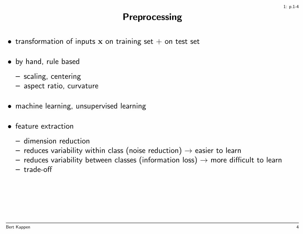
Preprocessing
• transformation of inputs x on training set + on test set
• by hand, rule based
– scaling, centering– aspect ratio, curvature
• machine learning, unsupervised learning
• feature extraction
– dimension reduction– reduces variability within class (noise reduction) → easier to learn– reduces variability between classes (information loss) → more difficult to learn– trade-off
Bert Kappen 4
1: p.1-4
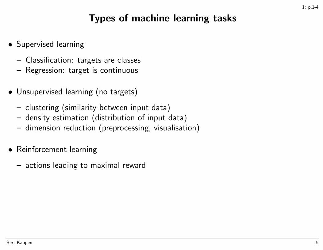
Types of machine learning tasks
• Supervised learning
– Classification: targets are classes– Regression: target is continuous
• Unsupervised learning (no targets)
– clustering (similarity between input data)– density estimation (distribution of input data)– dimension reduction (preprocessing, visualisation)
• Reinforcement learning
– actions leading to maximal reward
Bert Kappen 5
1.1: p.4-6
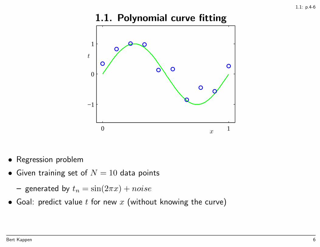
1.1. Polynomial curve fitting
x
t
0 1
−1
0
1
• Regression problem
• Given training set of N = 10 data points
– generated by tn = sin(2πx) + noise
• Goal: predict value t for new x (without knowing the curve)
Bert Kappen 6
1.1: p.4-6
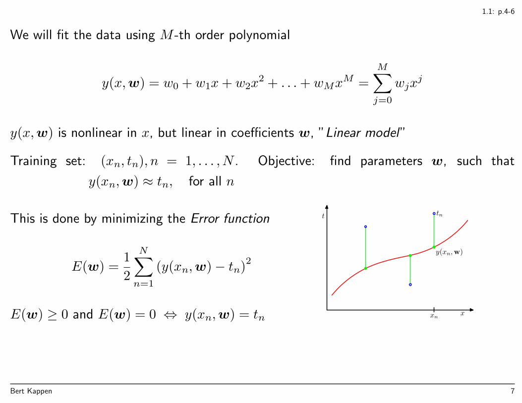
We will fit the data using M -th order polynomial
y(x,w) = w0 + w1x+ w2x2 + . . .+ wMx
M =
M∑j=0
wjxj
y(x,w) is nonlinear in x, but linear in coefficients w, ”Linear model”
Training set: (xn, tn), n = 1, . . . , N . Objective: find parameters w, such that
y(xn,w) ≈ tn, for all n
This is done by minimizing the Error function
E(w) =1
2
N∑n=1
(y(xn,w)− tn)2
E(w) ≥ 0 and E(w) = 0 ⇔ y(xn,w) = tn
t
x
y(xn,w)
tn
xn
Bert Kappen 7
math recap for 1.1: p.4-6
Partial derivatives, gradient, Nabla symbol
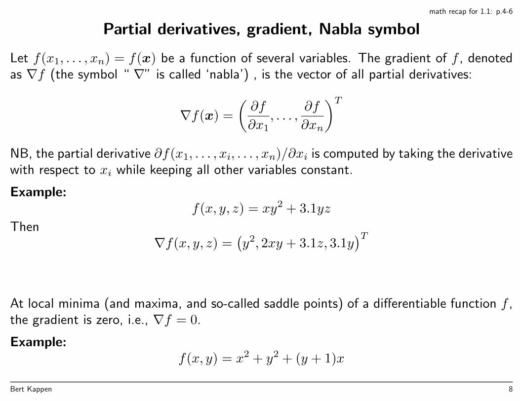
Let f(x1, . . . , xn) = f(x) be a function of several variables. The gradient of f , denotedas ∇f (the symbol “ ∇” is called ‘nabla’) , is the vector of all partial derivatives:
∇f(x) =
(∂f
∂x1, . . . ,
∂f
∂xn
)TNB, the partial derivative ∂f(x1, . . . , xi, . . . , xn)/∂xi is computed by taking the derivativewith respect to xi while keeping all other variables constant.
Example:f(x, y, z) = xy2 + 3.1yz
Then∇f(x, y, z) =
(y2, 2xy + 3.1z, 3.1y
)T
At local minima (and maxima, and so-called saddle points) of a differentiable function f ,the gradient is zero, i.e., ∇f = 0.
Example:f(x, y) = x2 + y2 + (y + 1)x
Bert Kappen 8

math recap for 1.1: p.4-6
So∇f(x, y) = (2x+ y + 1, 2y + x)
T
Then we can compute the point (x∗, y∗) that minimizes f by setting ∇f = 0,
2x∗ + y∗ + 1 = 02y∗ + x∗ = 0
⇒ (x∗, y∗) = (−2
3,1
3)
Bert Kappen 9

math recap for 1.1: p.4-6
Chain rule
Suppose f is a function of y1, y2, ..., yk and each yj is a function of x, then we cancompute the derivative of f with respect to x by the chain rule
df
dx=
k∑j=1
∂f
∂yj
dyjdx
Example:f(y(x), z(x)) = y(x)/z(x)
and y(x) = x4 and z = x2 then
df
dx=
1
z(x)y′(x)− y(x)
z(x)2z′(x) = 2x
Bert Kappen 10
math recap for 1.1: p.4-6
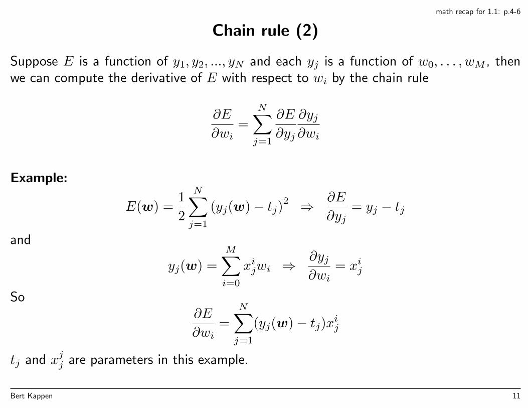
Chain rule (2)
Suppose E is a function of y1, y2, ..., yN and each yj is a function of w0, . . . , wM , thenwe can compute the derivative of E with respect to wi by the chain rule
∂E
∂wi=
N∑j=1
∂E
∂yj
∂yj∂wi
Example:
E(w) =1
2
N∑j=1
(yj(w)− tj)2 ⇒ ∂E
∂yj= yj − tj
and
yj(w) =
M∑i=0
xijwi ⇒∂yj∂wi
= xij
So∂E
∂wi=
N∑j=1
(yj(w)− tj)xij
tj and xjj are parameters in this example.
Bert Kappen 11
math recap for 1.1: p.4-6
Minimization of the error function
E(w) =1
2
N∑n=1
(y(xn,w)− tn)2
In minimum: gradient ∇wE = 0
Note: y linear in w ⇒ E quadratic in w
⇒ ∇wE is linear in w
⇒ ∇wE = 0: coupled set of linear equations (exercise)
Bert Kappen 12

math recap, see also app. C
Matrix multiplications as summations
If A is a N ×M matrix with entries Aij and v an M -dimensional vector with entries vi,then w = Av is a N -dimensional vector with components
wi =
M∑j=1
Aijvj
Similarly, if B is a M ×K matrix with entries Bij, then C = AB is a N ×K matrixwith entries
Cik =
M∑j=1
AijBjk
Bert Kappen 13
math recap, see also app. C
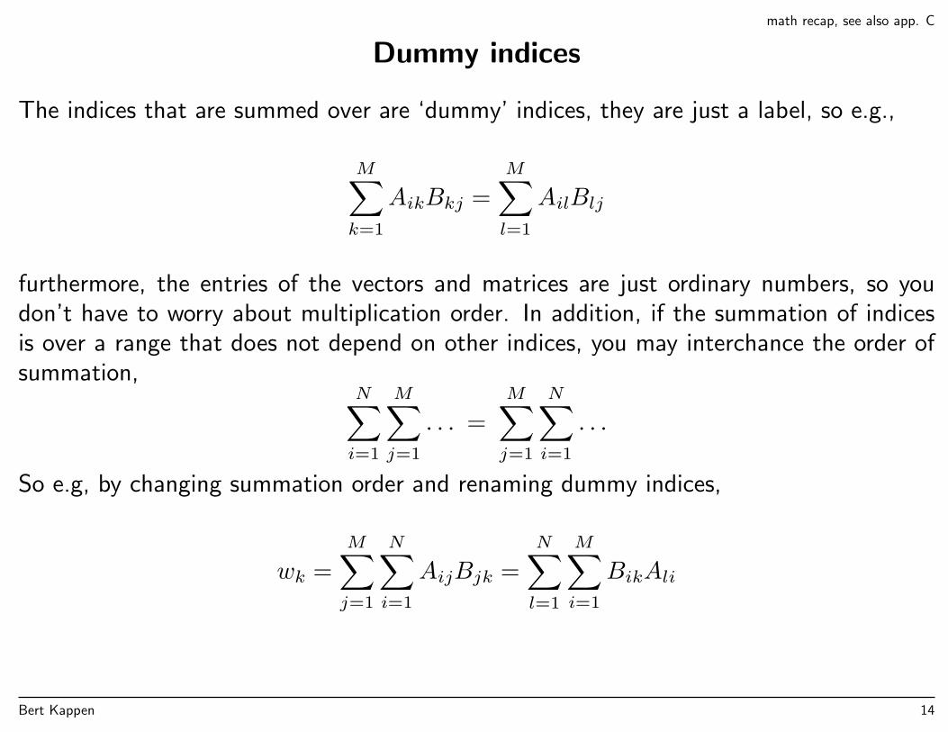
Dummy indices
The indices that are summed over are ‘dummy’ indices, they are just a label, so e.g.,
M∑k=1
AikBkj =
M∑l=1
AilBlj
furthermore, the entries of the vectors and matrices are just ordinary numbers, so youdon’t have to worry about multiplication order. In addition, if the summation of indicesis over a range that does not depend on other indices, you may interchance the order ofsummation,
N∑i=1
M∑j=1
. . . =
M∑j=1
N∑i=1
. . .
So e.g, by changing summation order and renaming dummy indices,
wk =
M∑j=1
N∑i=1
AijBjk =
N∑l=1
M∑i=1
BikAli
Bert Kappen 14
math recap, see also app. C
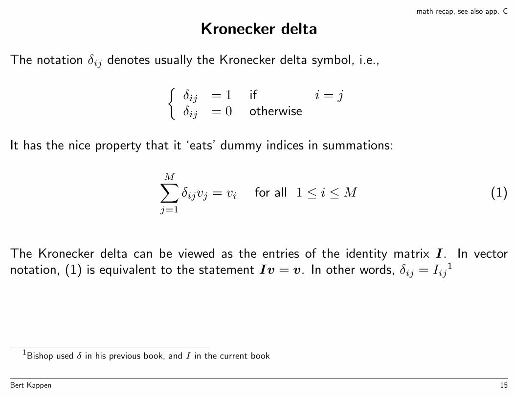
Kronecker delta
The notation δij denotes usually the Kronecker delta symbol, i.e.,δij = 1 if i = jδij = 0 otherwise
It has the nice property that it ‘eats’ dummy indices in summations:
M∑j=1
δijvj = vi for all 1 ≤ i ≤M (1)
The Kronecker delta can be viewed as the entries of the identity matrix I. In vectornotation, (1) is equivalent to the statement Iv = v. In other words, δij = Iij
1
1Bishop used δ in his previous book, and I in the current book
Bert Kappen 15
math recap, needed later
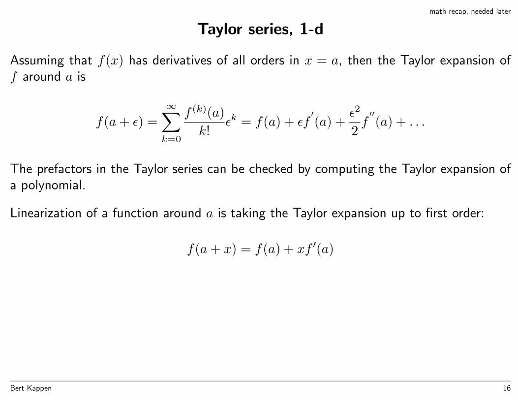
Taylor series, 1-d
Assuming that f(x) has derivatives of all orders in x = a, then the Taylor expansion off around a is
f(a+ ε) =
∞∑k=0
f (k)(a)
k!εk = f(a) + εf
′(a) +
ε2
2f′′(a) + . . .
The prefactors in the Taylor series can be checked by computing the Taylor expansion ofa polynomial.
Linearization of a function around a is taking the Taylor expansion up to first order:
f(a+ x) = f(a) + xf ′(a)
Bert Kappen 16
math recap
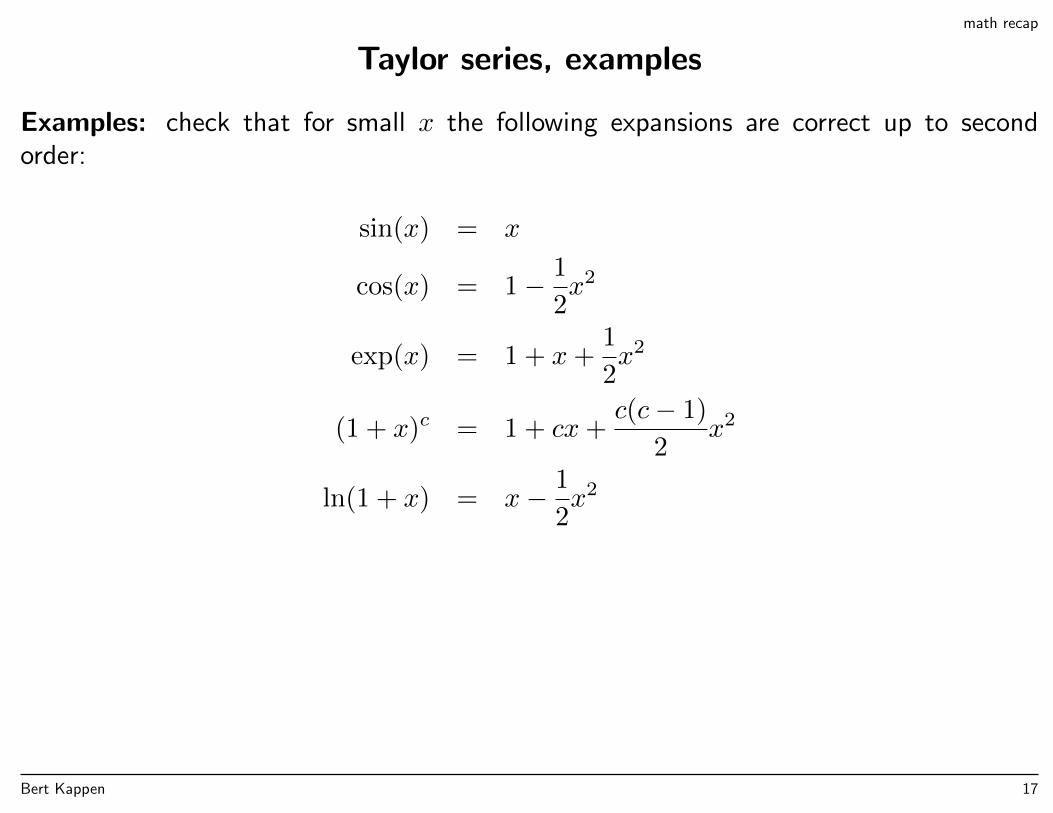
Taylor series, examples
Examples: check that for small x the following expansions are correct up to secondorder:
sin(x) = x
cos(x) = 1− 1
2x2
exp(x) = 1 + x+1
2x2
(1 + x)c = 1 + cx+c(c− 1)
2x2
ln(1 + x) = x− 1
2x2
Bert Kappen 17
math recap, needed later
Taylor expansion in several dimensions
The Taylor expansion of a function of several variables, f(x1, . . . , xn) = f(x) is (up tosecond order)
f(x) = f(a) +∑i
(xi − ai)∂
∂xif(a) +
1
2
∑ij
(xi − ai)(xj − aj)∂
∂xi
∂
∂xjf(a)
or in vector notation, with ε = x− a
f(a+ ε) = f(a) + εT∇f(a) +1
2εTHε
with H the Hessian, which is the symmetric matrix of partial derivatives
Hij =∂2
∂xi∂xjf(x)
∣∣∣∣x=a
Bert Kappen 18
This is not in ch 1, but is an important concept in SML - ch 5.2.1
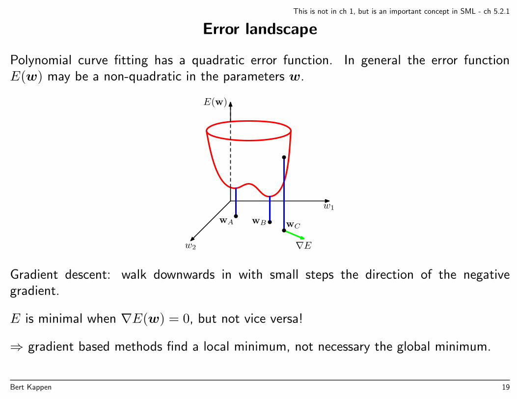
Error landscape
Polynomial curve fitting has a quadratic error function. In general the error functionE(w) may be a non-quadratic in the parameters w.
w1
w2
E(w)
wA wB wC
∇E
Gradient descent: walk downwards in with small steps the direction of the negativegradient.
E is minimal when ∇E(w) = 0, but not vice versa!
⇒ gradient based methods find a local minimum, not necessary the global minimum.
Bert Kappen 19
This is not in ch 1, but is an important concept in SML - ch 5.2.4
Application: Optimization by gradient descent
Gradient descent algorithm:
1. Start with an initial value of w and ε small.
2. While ”change in w large”: Compute w := w − ε∇E
Stop criterion is ∇E ≈ 0, which means that we stop in a local minimum of E.
Does this algorithm converge? Yes, if ε is ”sufficiently small” and E bounded from below.
Proof: Denote ∆w = −ε∇E.
E(w + ∆w) ≈ E(w) + (∆w)T∇E = E(w)− ε∑i
( ∂E∂wi
)2 ≤ E(w)
In each gradient descent step the value of E is lowered. Since E bounded from below,the procedure must converge asymptotically.
Bert Kappen 20
This is not in ch 1, but is an important concept in SML - ch 5.2.2
Newtons method
One can also use Hessian information for optimization. As an example, consider aquadratic approximation to E around w0:
E(w) = E(w0) + bT (w −w0) +1
2(w −w0)H(w −w0)
bi =∂E(w0)
∂wiHij =
∂2E(w0)
∂wi∂wj
∇E(w) = b+H(w −w0)
We can solve ∇E(w) = 0 and obtain
w = w0 −H−1∇E(w0)
This is called Newtons method. Inversion of the Hessian may be computational costly.A number of methods, known as quasi-newton methods, are based on approximations ofthis procedure.
Bert Kappen 21

1.1: p 6-11
Model comparison, model selection
Back to polynomial curve fitting: how to choose M?
x
t
M = 0
0 1
−1
0
1
x
t
M = 1
0 1
−1
0
1
x
t
M = 3
0 1
−1
0
1
x
t
M = 9
0 1
−1
0
1
Which of these models is the best one?
Bert Kappen 22

1.1: p 6-11
Define root-mean-square error on training set and on test set (xn, tn)Nn=1, respectively:
ERMS =√
2E(w∗)/N, ERMS =
√√√√ 1
N
N∑n=1
(y(xn,w∗)− tn
)2
M
ERMS
0 3 6 90
0.5
1TrainingTest
Too simple (small M) → poor fitToo complex (large M) → overfitting (fits the noise)Note that series expansion of sin contain terms of all orders.
Bert Kappen 23
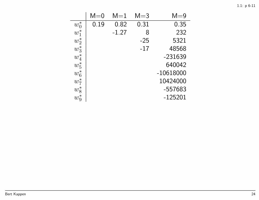
1.1: p 6-11
M=0 M=1 M=3 M=9w∗0 0.19 0.82 0.31 0.35w∗1 -1.27 8 232w∗2 -25 5321w∗3 -17 48568w∗4 -231639w∗5 640042w∗6 -10618000w∗7 10424000w∗8 -557683w∗9 -125201
Bert Kappen 24
1.1: p 6-11
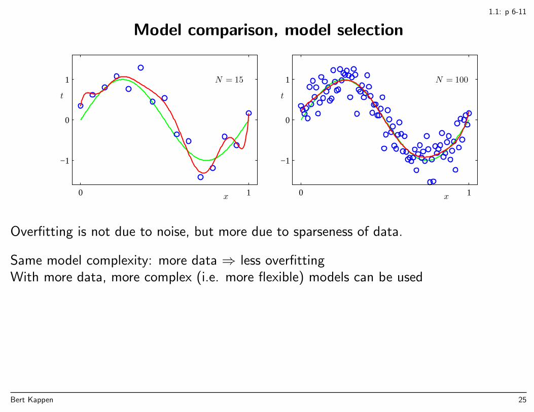
Model comparison, model selection
x
t
N = 15
0 1
−1
0
1
x
t
N = 100
0 1
−1
0
1
Overfitting is not due to noise, but more due to sparseness of data.
Same model complexity: more data ⇒ less overfittingWith more data, more complex (i.e. more flexible) models can be used
Bert Kappen 25
1.1: p 6-11
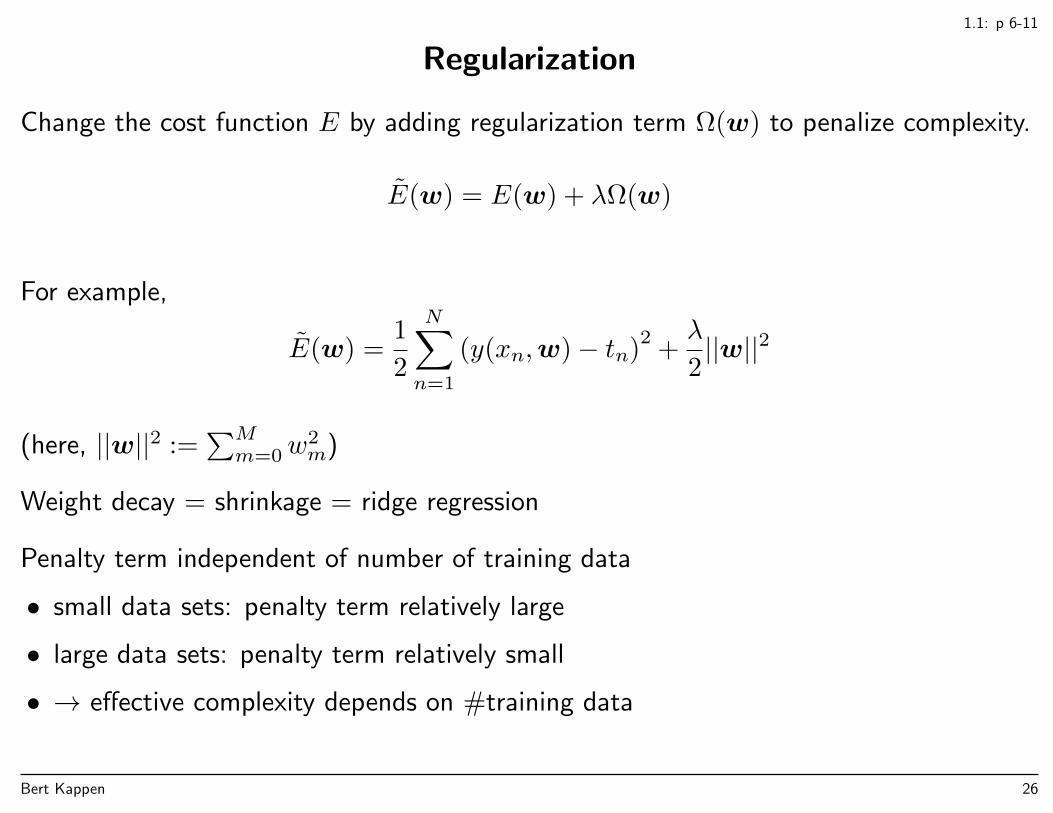
Regularization
Change the cost function E by adding regularization term Ω(w) to penalize complexity.
E(w) = E(w) + λΩ(w)
For example,
E(w) =1
2
N∑n=1
(y(xn,w)− tn)2
+λ
2||w||2
(here, ||w||2 :=∑Mm=0w
2m)
Weight decay = shrinkage = ridge regression
Penalty term independent of number of training data
• small data sets: penalty term relatively large
• large data sets: penalty term relatively small
• → effective complexity depends on #training data
Bert Kappen 26
1.1: p 6-11
x
t
M = 9
0 1
−1
0
1
x
t
ln λ = −18
0 1
−1
0
1
x
t
ln λ = 0
0 1
−1
0
1
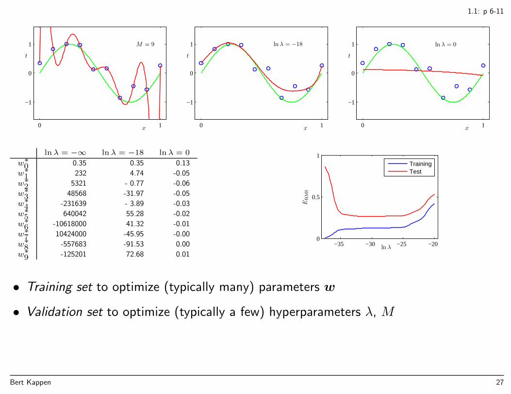
lnλ = −∞ lnλ = −18 lnλ = 0
w∗0 0.35 0.35 0.13
w∗1 232 4.74 -0.05
w∗2 5321 - 0.77 -0.06
w∗3 48568 -31.97 -0.05
w∗4 -231639 - 3.89 -0.03
w∗5 640042 55.28 -0.02
w∗6 -10618000 41.32 -0.01
w∗7 10424000 -45.95 -0.00
w∗8 -557683 -91.53 0.00
w∗9 -125201 72.68 0.01
ERMS
ln λ−35 −30 −25 −200
0.5
1TrainingTest
• Training set to optimize (typically many) parameters w
• Validation set to optimize (typically a few) hyperparameters λ, M
Bert Kappen 27
1.2: p 12-17
Probability theory
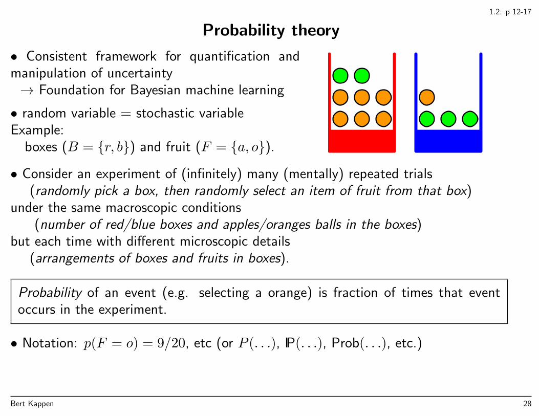
• Consistent framework for quantification andmanipulation of uncertainty→ Foundation for Bayesian machine learning
• random variable = stochastic variableExample:
boxes (B = r, b) and fruit (F = a, o).
• Consider an experiment of (infinitely) many (mentally) repeated trials(randomly pick a box, then randomly select an item of fruit from that box)
under the same macroscopic conditions(number of red/blue boxes and apples/oranges balls in the boxes)
but each time with different microscopic details(arrangements of boxes and fruits in boxes).
Probability of an event (e.g. selecting a orange) is fraction of times that eventoccurs in the experiment.
• Notation: p(F = o) = 9/20, etc (or P (. . .), IP(. . .), Prob(. . .), etc.)
Bert Kappen 28
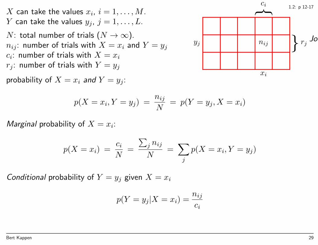
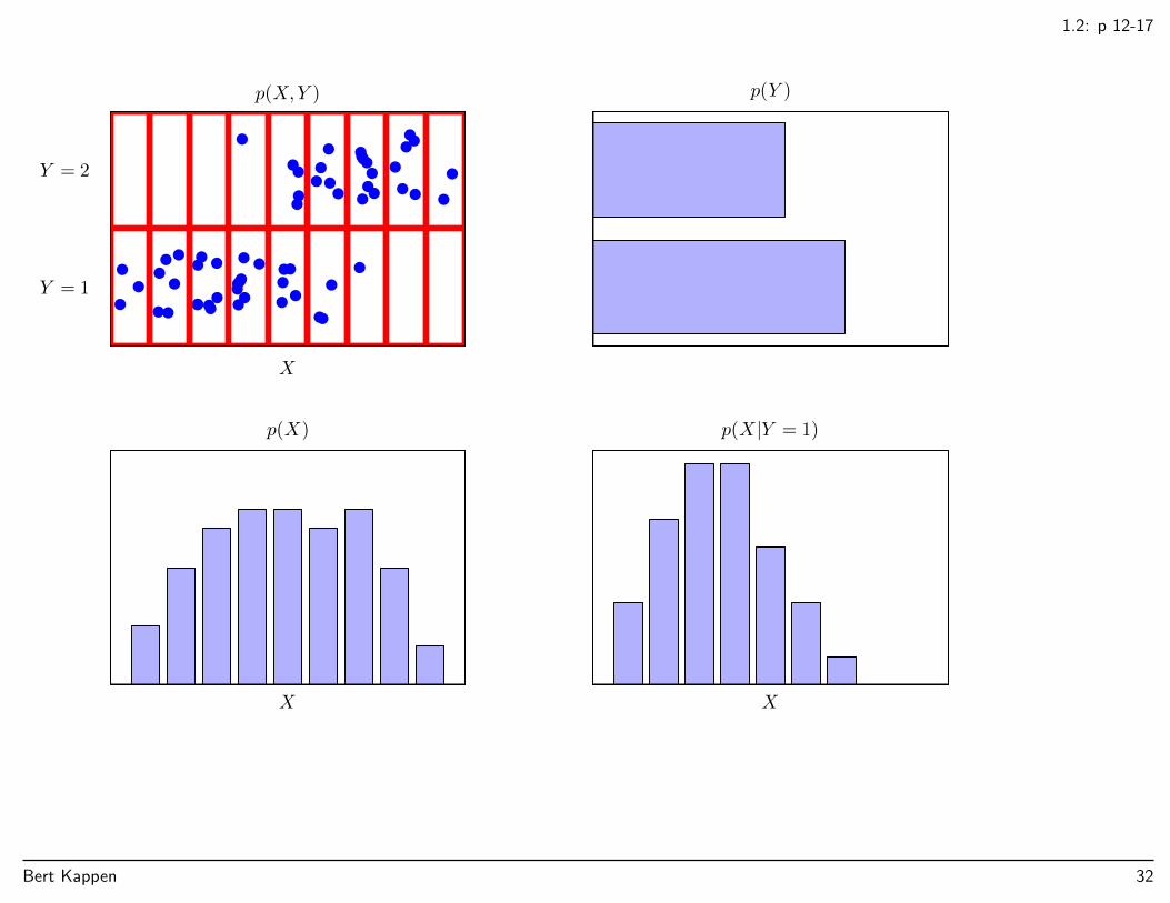
1.2: p 12-17X can take the values xi, i = 1, . . . ,M .Y can take the values yj, j = 1, . . . , L.
N : total number of trials (N →∞).nij: number of trials with X = xi and Y = yjci: number of trials with X = xirj: number of trials with Y = yj
ci
rjyj
xi
nijJoint
probability of X = xi and Y = yj:
p(X = xi, Y = yj) =nijN
= p(Y = yj, X = xi)
Marginal probability of X = xi:
p(X = xi) =ciN
=
∑j nij
N=∑j
p(X = xi, Y = yj)
Conditional probability of Y = yj given X = xi
p(Y = yj|X = xi) =nijci
Bert Kappen 29
1.2: p 12-17
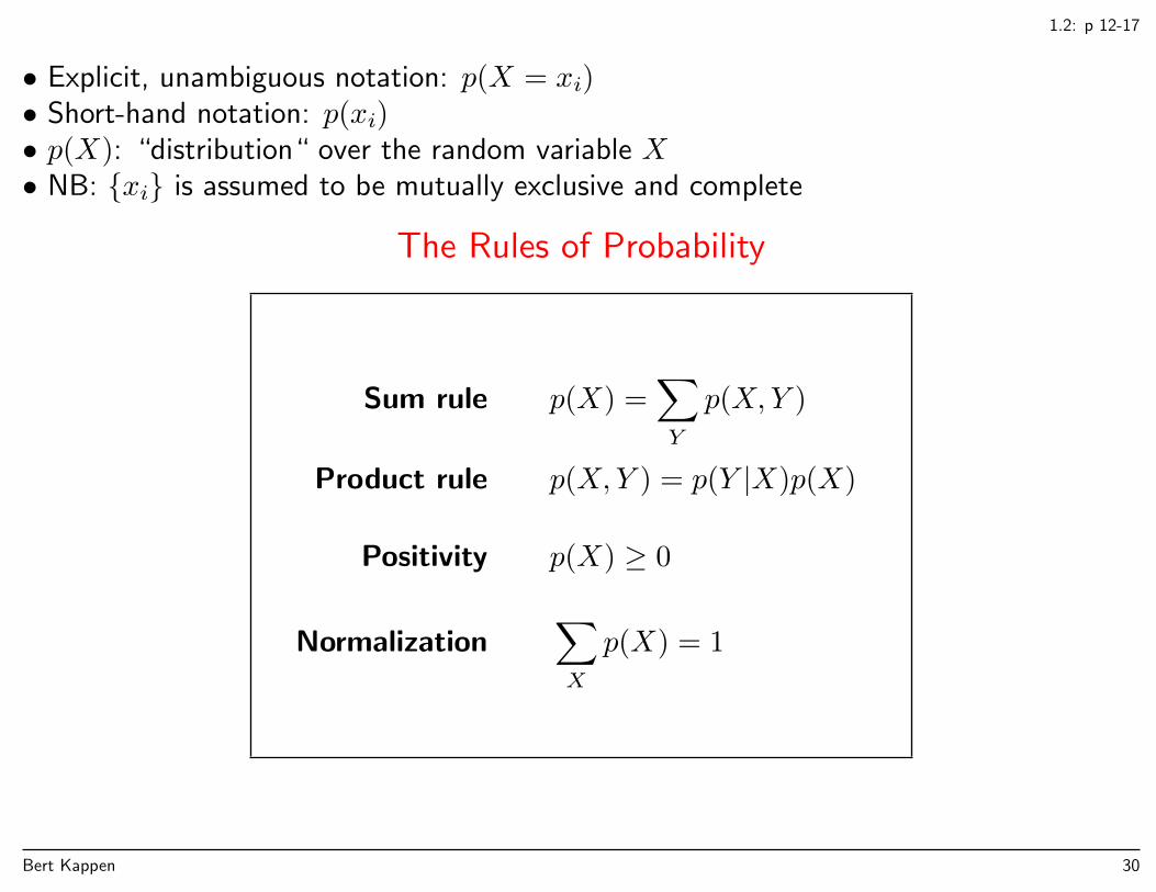
• Explicit, unambiguous notation: p(X = xi)• Short-hand notation: p(xi)• p(X): “distribution“ over the random variable X• NB: xi is assumed to be mutually exclusive and complete
The Rules of Probability
Sum rule p(X) =∑Y
p(X,Y )
Product rule p(X,Y ) = p(Y |X)p(X)
Positivity p(X) ≥ 0
Normalization∑X
p(X) = 1
Bert Kappen 30
1.2: p 12-17
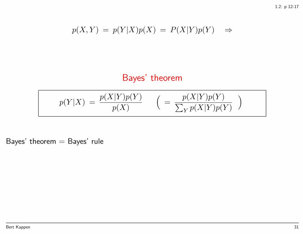
p(X,Y ) = p(Y |X)p(X) = P (X|Y )p(Y ) ⇒
Bayes’ theorem
p(Y |X) =p(X|Y )p(Y )
p(X)
(=
p(X|Y )p(Y )∑Y p(X|Y )p(Y )
)
Bayes’ theorem = Bayes’ rule
Bert Kappen 31
1.2: p 12-17
p(X,Y )
X
Y = 2
Y = 1
p(Y )
p(X)
X X
p(X |Y = 1)
Bert Kappen 32
1.2: p 12-17
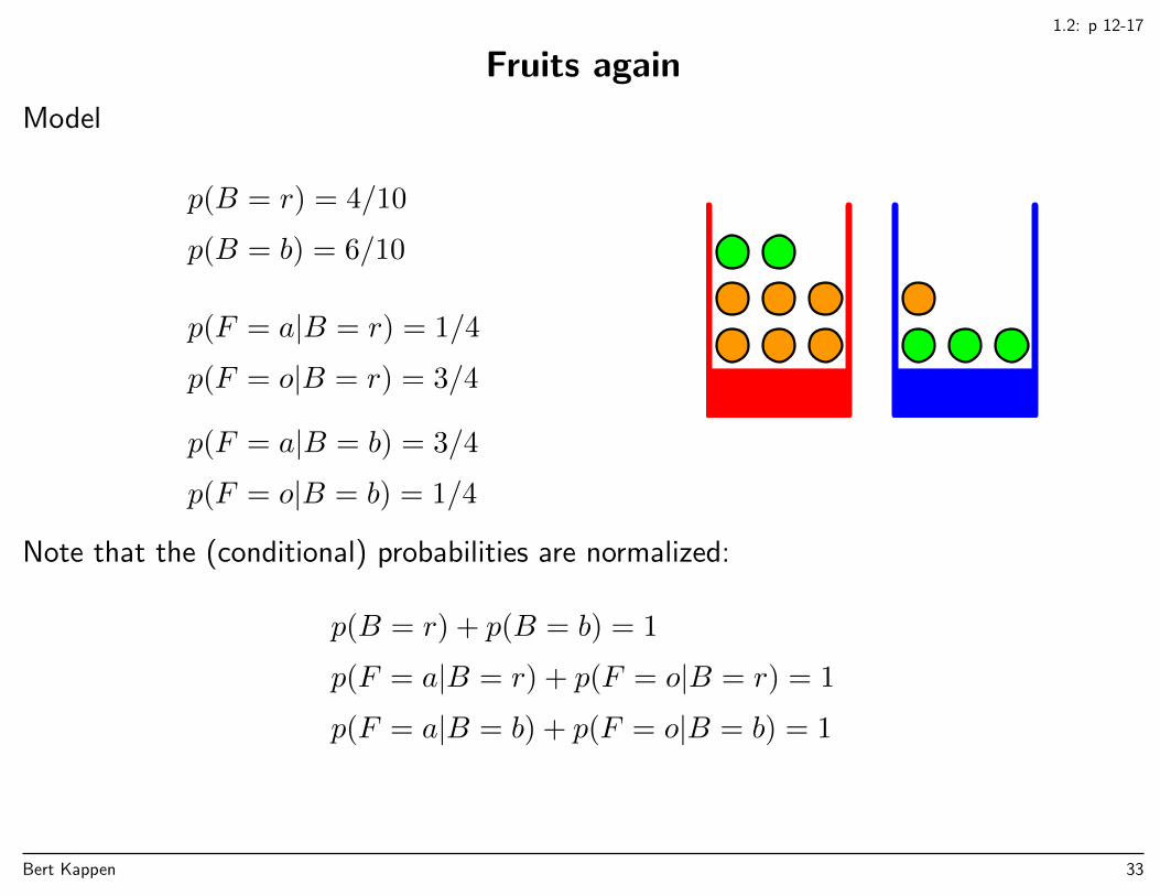
Fruits again
Model
p(B = r) = 4/10
p(B = b) = 6/10
p(F = a|B = r) = 1/4
p(F = o|B = r) = 3/4
p(F = a|B = b) = 3/4
p(F = o|B = b) = 1/4
Note that the (conditional) probabilities are normalized:
p(B = r) + p(B = b) = 1
p(F = a|B = r) + p(F = o|B = r) = 1
p(F = a|B = b) + p(F = o|B = b) = 1
Bert Kappen 33
1.2: p 12-17
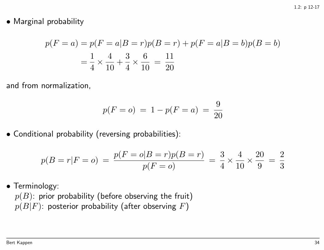
• Marginal probability
p(F = a) = p(F = a|B = r)p(B = r) + p(F = a|B = b)p(B = b)
=1
4× 4
10+
3
4× 6
10=
11
20
and from normalization,
p(F = o) = 1− p(F = a) =9
20
• Conditional probability (reversing probabilities):
p(B = r|F = o) =p(F = o|B = r)p(B = r)
p(F = o)=
3
4× 4
10× 20
9=
2
3
• Terminology:p(B): prior probability (before observing the fruit)p(B|F ): posterior probability (after observing F )
Bert Kappen 34
1.2: p 12-17
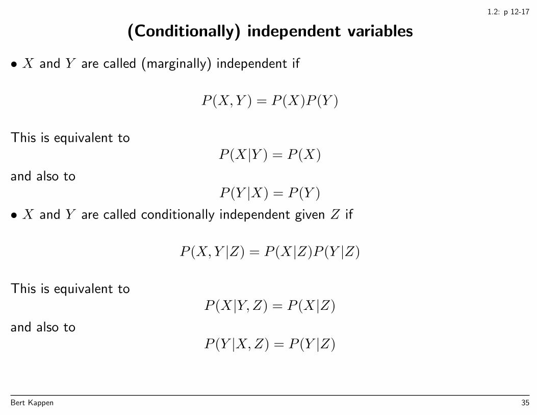
(Conditionally) independent variables
• X and Y are called (marginally) independent if
P (X,Y ) = P (X)P (Y )
This is equivalent toP (X|Y ) = P (X)
and also toP (Y |X) = P (Y )
• X and Y are called conditionally independent given Z if
P (X,Y |Z) = P (X|Z)P (Y |Z)
This is equivalent toP (X|Y,Z) = P (X|Z)
and also toP (Y |X,Z) = P (Y |Z)
Bert Kappen 35
1.2.1
Probability densities
• to deal with continuous variables (rather than discrete var’s)
When x takes values from a continuous domain, the probability of any value of x is zero!Instead, we must talk of the probability that x takes a value in a certain interval
Prob(x ∈ [a, b]) =
∫ b
a
p(x) dx
with p(x) the probability density over x.
p(x) ≥ 0∫ ∞−∞
p(x) dx = 1 (normalization)
• NB: that p(x) may be bigger than one.
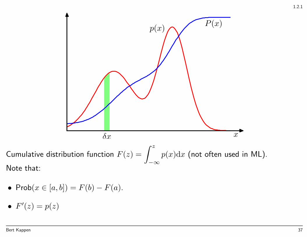
Probability of x falling in interval (x, x+ δx) is p(x)δx for δx→ 0
Bert Kappen 36
1.2.1
xδx
p(x) P (x)
Cumulative distribution function F (z) =
∫ z
−∞p(x)dx (not often used in ML).
Note that:
• Prob(x ∈ [a, b]) = F (b)− F (a).
• F ′(z) = p(z)
Bert Kappen 37
1.2.1
Multivariate densities
• Several continuous variables, denoted by the d dimensional vector x = (x1, . . . , xd).• Probability density p(x): probability of x falling in an infinitesimal volume δx aroundx is given by p(x)δx.
Prob(x ∈ R) =
∫Rp(x) dx =
∫Rp(x1, . . . , xd)dx1dx2 . . . dxd
and
p(x) ≥ 0∫p(x)dx = 1
• Rules of probability apply to continuous variables as well,
p(x) =
∫p(x, y) dy
p(x, y) = p(y|x)p(x)
Bert Kappen 38

math recap for 1.2.1
Integration
The integral of a function of several variables x = (x1, x2, . . . , xn)∫Rf(x)dx ≡
∫Rf(x1, x2, . . . , xn)dx1dx2 . . . dxn
is the volume of the n + 1 dimensional region lying ‘vertically above’ the domain ofintegration R ⊂ IRn and ’below’ the function f(x).
Bert Kappen 39
math recap for 1.2.1
Separable integrals
The most easy (but important) case is when we can separate the integration, e.g. in 2-d,
∫ b
x=a
∫ d
y=c
f(x)g(y) dxdy =
∫ b
x=a
f(x) dx
∫ d
y=c
g(y) dy
Example,
∫exp
( n∑i=1
fi(xi))
dx =
∫ n∏i=1
exp(fi(xi)) dx =
n∏i=1
∫exp(fi(xi)) dxi
Bert Kappen 40
math recap
Iterated integration
A little more complicated are the cases, in which integration can be done by iteration,’from inside out’. Suppose we can write the 2-d region R as the set a < x < b andc(x) < y < d(x) then we can write
∫Rf(y, x) dydx =
∫ b
x=a
[∫ d(x)
y=c(x)
f(y, x) dy
]dx
The first step is evaluate the inner integral, where we interpret f(y, x) as a function of ywith fixed parameter x. Suppose we can find F such that ∂F (y, x)/∂y = f(y, x), thenthe result of the inner integral is
∫ d(x)
y=c(x)
f(y, x) dy = F (d(x), x)− F (c(x), x)
The result, which we call g(x) is obviously a function of x only,
g(x) ≡ F (d(x), x)− F (c(x), x)
Bert Kappen 41
math recap
The next step is the outer integral, which is now just a one-dimensional integral of thefunction g, ∫ b
x=a
[∫ d(x)
y=c(x)
f(y, x) dy
]dx =
∫ b
x=a
g(x) dx
Now suppose that the same 2-d region R can also be written as the set s < y < t andu(y) < x < v(y), then we can also choose to evaluate the integral as
∫Rf(y, x) dxdy =
∫ t
y=s
[∫ v(y)
x=u(y)
f(y, x) dx
]dy
following the same procedure as above. In most regular cases the result is the same (forexceptions, see handout (*)).
Integration with more than two variables can be done with exactly the same procedure,‘from inside out’.
In Machine Learning, integration is mostly over the whole of x space, or over a subspace.Iterated integration is not often used.
Bert Kappen 42
math recap
Transformation of variables (1-d)
Often it is easier to do the multidimensional integral in another coordinate frame. Supposewe want to do the integration ∫ d
y=c
f(y) dy
but the function f(y) is easier expressed as a f(y(x)) which is a function of x. So wewant to use x as integration variable. If y and x are related via invertible differentiablemappings y = y(x) and x = x(y) and the end points of the interval (y = c, y = d) aremapped to (x = a, x = b), (so c = y(a), etc) then we have the equality∫ d
y=c
f(y) dy =
∫ d
y(x)=c
f(y(x)) dy(x)
=
∫ b
x=a
f(y(x))y′(x) dx
The derivative y′(x) comes in as the ratio between the lengths of the differentials dy anddx,
dy = y′(x) dx
Bert Kappen 43
math recap
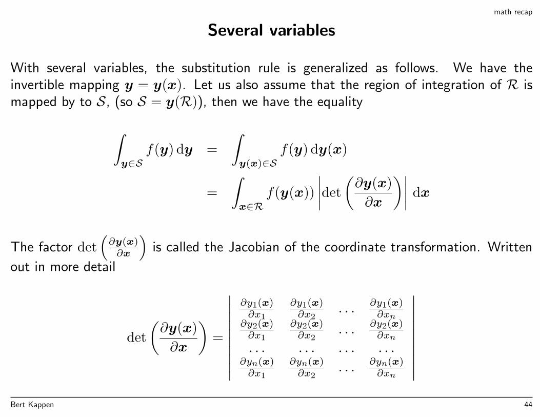
Several variables
With several variables, the substitution rule is generalized as follows. We have theinvertible mapping y = y(x). Let us also assume that the region of integration of R ismapped by to S, (so S = y(R)), then we have the equality
∫y∈S
f(y) dy =
∫y(x)∈S
f(y) dy(x)
=
∫x∈R
f(y(x))
∣∣∣∣det
(∂y(x)
∂x
)∣∣∣∣ dx
The factor det(∂y(x)∂x
)is called the Jacobian of the coordinate transformation. Written
out in more detail
det
(∂y(x)
∂x
)=
∣∣∣∣∣∣∣∣∣∣
∂y1(x)∂x1
∂y1(x)∂x2
. . . ∂y1(x)∂xn
∂y2(x)∂x1
∂y2(x)∂x2
. . . ∂y2(x)∂xn
. . . . . . . . . . . .∂yn(x)∂x1
∂yn(x)∂x2
. . . ∂yn(x)∂xn
∣∣∣∣∣∣∣∣∣∣Bert Kappen 44
math recap
The absolute value 2 of the Jacobian comes in as the ratio between that the volumerepresented by the differential dy and the volume represented by the differential dx, i.e.,
dy =
∣∣∣∣det
(∂y(x)
∂x
)∣∣∣∣ dx
As a last remark, it is good to know that
det
(∂x(y)
∂y
)= det
((∂y(x)
∂x
)−1)
=1
det(∂y(x)∂x
)
2In the single-variable case, we took the orientation of the integration interval into account (∫ ba f(x) dx = −
∫ ab f(x) dx).
With several variables, this is awkward. Fortunately, it turns out that the orientation of the mapping of the domain alwayscancels to the ’orientation’ of the Jacobian (= sign of the determinant). Therefore we take a positive orientation and theabsolute value of the Jacobian
Bert Kappen 45
math recap
Polar coordinates
Example: compute the area of a disc.
Consider a two-dimensional disc with radius R
D = (x, y)|x2 + y2 < R2
Its area is ∫D
dxdy
This integral is easiest evaluated by going to ‘polar-coordinates’. The mapping from polarcoordinates (r, θ) to Cartesian coordinates (x, y) is
x = r cos θ (2)
y = r sin θ (3)
Since In polar coordinates, the disc is described by 0 ≤ r < R (since x2 + y2 = r2) and0 ≤ θ < 2π.
Bert Kappen 46

math recap
The Jacobian is
J =
∣∣∣∣ ∂x∂r
∂x∂θ
∂y∂r
∂y∂θ
∣∣∣∣ =
∣∣∣∣ cos θ −r sin θsin θ r cos θ
∣∣∣∣ = r(cos2 θ + sin2 θ) = r
In other words,dxdy = rdrdθ
The area of the disc is now easily evaluated.
∫D
dxdy =
∫ 2π
θ=0
∫ R
r=0
rdrdθ = πR2
Bert Kappen 47
math recap
Gaussian integral
How to compute ∫ ∞−∞
exp(−x2)dx
(∫ ∞−∞
exp(−x2)dx)2
=
∫ ∞−∞
exp(−x2)dx
∫ ∞−∞
exp(−y2)dy
=
∫ ∞−∞
∫ ∞−∞
exp(−x2) exp(−y2)dxdy
=
∫ ∞−∞
∫ ∞−∞
exp(−(x2 + y2))dxdy
Bert Kappen 48
math recap
The latter is easily evaluated by going to polar-coordinates,
∫ ∞−∞
∫ ∞−∞
exp(−(x2 + y2))dxdy =
∫ 2π
θ=0
∫ ∞r=0
exp(−r2)rdrdθ
= 2π
∫ ∞r=0
exp(−r2)rdr
= 2π ×(− 1
2exp(−r2)
)∣∣∣∞0
= π
So ∫ ∞−∞
exp(−x2)dx =√π
Bert Kappen 49
1.2.1: p.18
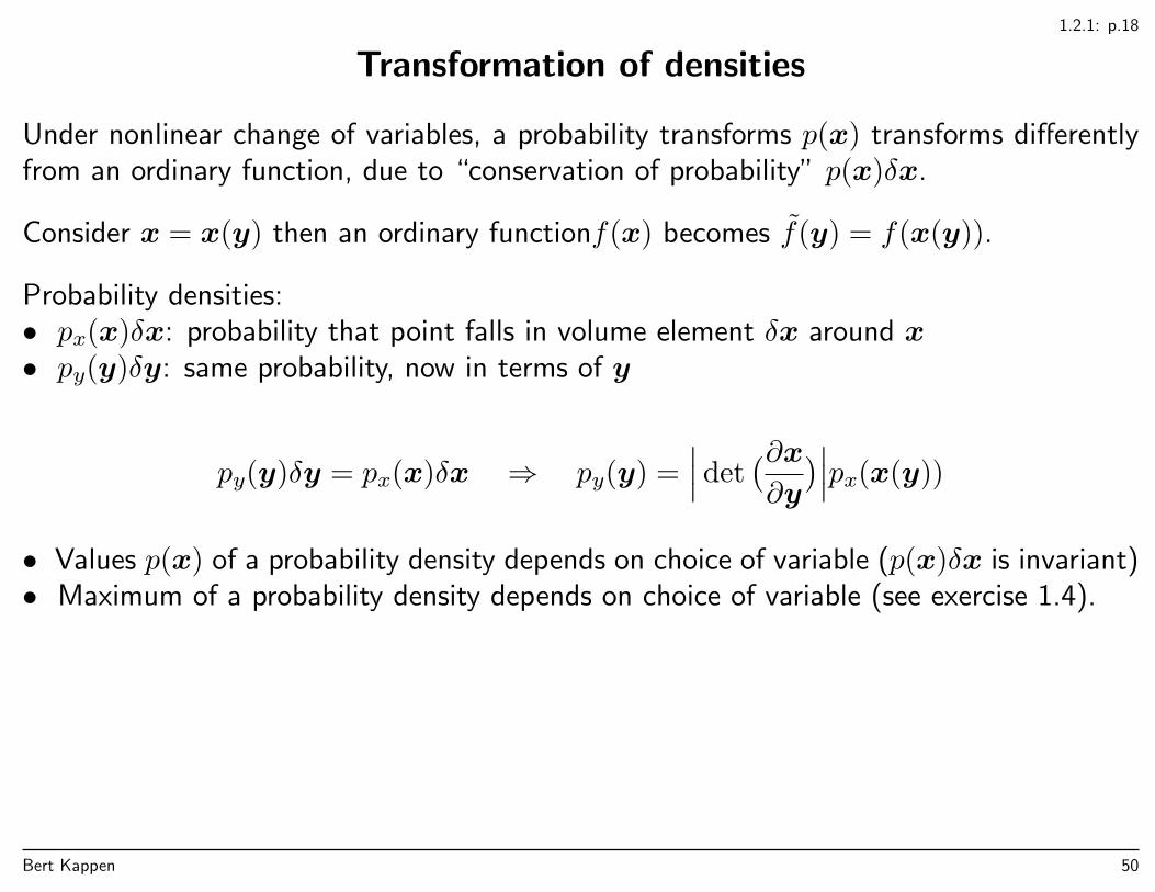
Transformation of densities
Under nonlinear change of variables, a probability transforms p(x) transforms differentlyfrom an ordinary function, due to “conservation of probability” p(x)δx.
Consider x = x(y) then an ordinary functionf(x) becomes f(y) = f(x(y)).
Probability densities:• px(x)δx: probability that point falls in volume element δx around x• py(y)δy: same probability, now in terms of y
py(y)δy = px(x)δx ⇒ py(y) =∣∣∣ det
(∂x∂y
)∣∣∣px(x(y))
• Values p(x) of a probability density depends on choice of variable (p(x)δx is invariant)• Maximum of a probability density depends on choice of variable (see exercise 1.4).
Bert Kappen 50
math recap
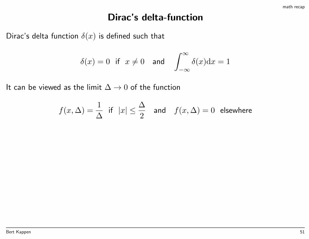
Dirac’s delta-function
Dirac’s delta function δ(x) is defined such that
δ(x) = 0 if x 6= 0 and
∫ ∞−∞
δ(x)dx = 1
It can be viewed as the limit ∆→ 0 of the function
f(x,∆) =1
∆if |x| ≤ ∆
2and f(x,∆) = 0 elsewhere
Bert Kappen 51

math recap
The Dirac delta δ(x) is a spike (a peak, a point mass) at x = 0. The function δ(x− x0)as a function of x is a spike at x0. As a consequence of the definition, the delta functionhas the important property ∫ ∞
−∞f(x)δ(x− x0)dx = f(x0)
(cf. Kronecker delta∑j δijvj = vi ).
The multivariate deltafunction factorizes over the dimensions
δ(x−m) =
n∏i=1
δ(xi −mi)
Bert Kappen 52
math recap
Dirac’s delta-function / delta-distribution
The Dirac delta is actually a distribution rather than a function:
δ(αx) =1
αδ(x)
This is true since
• if x 6= 0 left and right-handside are both zero.
• after transformation of variables x′ = αx, dx′ = αdx we have∫δ(αx)dx =
1
α
∫δ(x′)dx′ =
1
α
Bert Kappen 53
math recap for 1.2.2
Functionals vs functions
Function y: for any input value x, returns output value f(y).
Functional F : for any function y, returns an output value F [y].
Example (linear functional):
F [y] =
∫p(x)y(x) dx
(Compare with f(y) =∑i piyi).
Other (nonlinear) example:
F [y] =
∫1
2(y′(x) + V (x))2 dx
Bert Kappen 54
1.2.2
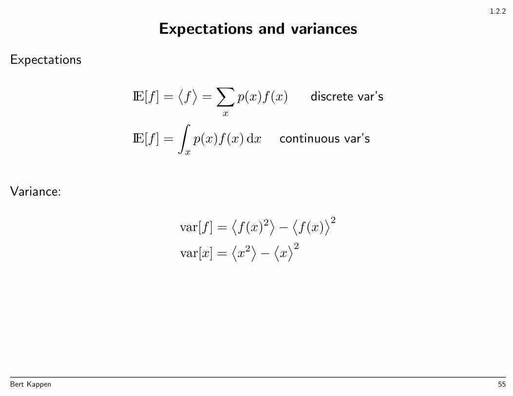
Expectations and variances
Expectations
IE[f ] =⟨f⟩
=∑x
p(x)f(x) discrete var’s
IE[f ] =
∫x
p(x)f(x) dx continuous var’s
Variance:
var[f ] =⟨f(x)2
⟩−⟨f(x)
⟩2var[x] =
⟨x2⟩−⟨x⟩2
Bert Kappen 55

1.2.2
Covariance
Covariance of two random variables
cov[x, y] = 〈xy〉 − 〈x〉 〈y〉
Covariance matrix of the components of a vector variable
cov[x] ≡ cov[x,x] =⟨xxT
⟩−⟨x⟩⟨xT⟩
with components
(cov[x])ij = cov[xi, xj] =⟨xixj
⟩−⟨xi⟩⟨xj⟩
Bert Kappen 56
1.2.3
Bayesian probabilities
• Classical or frequentists interpretation: probabilities in terms of frequencies of randomrepeatable events
• Bayesian view: probabilities as subjective beliefs about uncertain event
– event not neccessarily repeatable– event may yield only indirect observations– Bayesian inference to update belief given observations
Why probability theory?
• Cox: common sense axioms for degree of uncertainty → probability theory
• de Finetti: betting games with uncertain events → probability theory (otherwise facecertain loss through Dutch book)
Bert Kappen 57

1.2.3
Dutch book
Bert Kappen 58
1.2.3
Maximum likelihood estimation
Given a data set
Data = x1, . . . ,xN
and a parametrized distribution
p(x|w), w = (w1, . . . , wM),
find the value of w that best describes the data.
The common approach is to assume that the data that we observe are drawn independentlyfrom p(x|w) (independent and identical distributed = i.i.d.) for some unknown value ofw:
p(Data|w) = p(x1, . . . ,xN|w) =
N∏i=1
p(xi|w)
Bert Kappen 59
1.2.3
Then, the most likely w is obtained by maximizing p(Data|w) wrt w:
wML = argmaxwp(Data|w) = argmaxw
N∏i=1
p(xi|w)
= argmaxw
N∑i=1
log p(xi|w)
since log is a monotonically increasing function.
wML is a function of the data. This is called an estimator.
Frequentists methods consider a single true w and data generation mechanism p(Data|wprovided by ’Nature’ and study expected value:
EwML =∑Data
p(Data|w)wML(Data)
For instance, µ = 1N
∑i xi is estimator for the mean of a distribution. If data are
xi ∼ N (µ, σ2) then Eµ = µ.
Bert Kappen 60
1.2.3
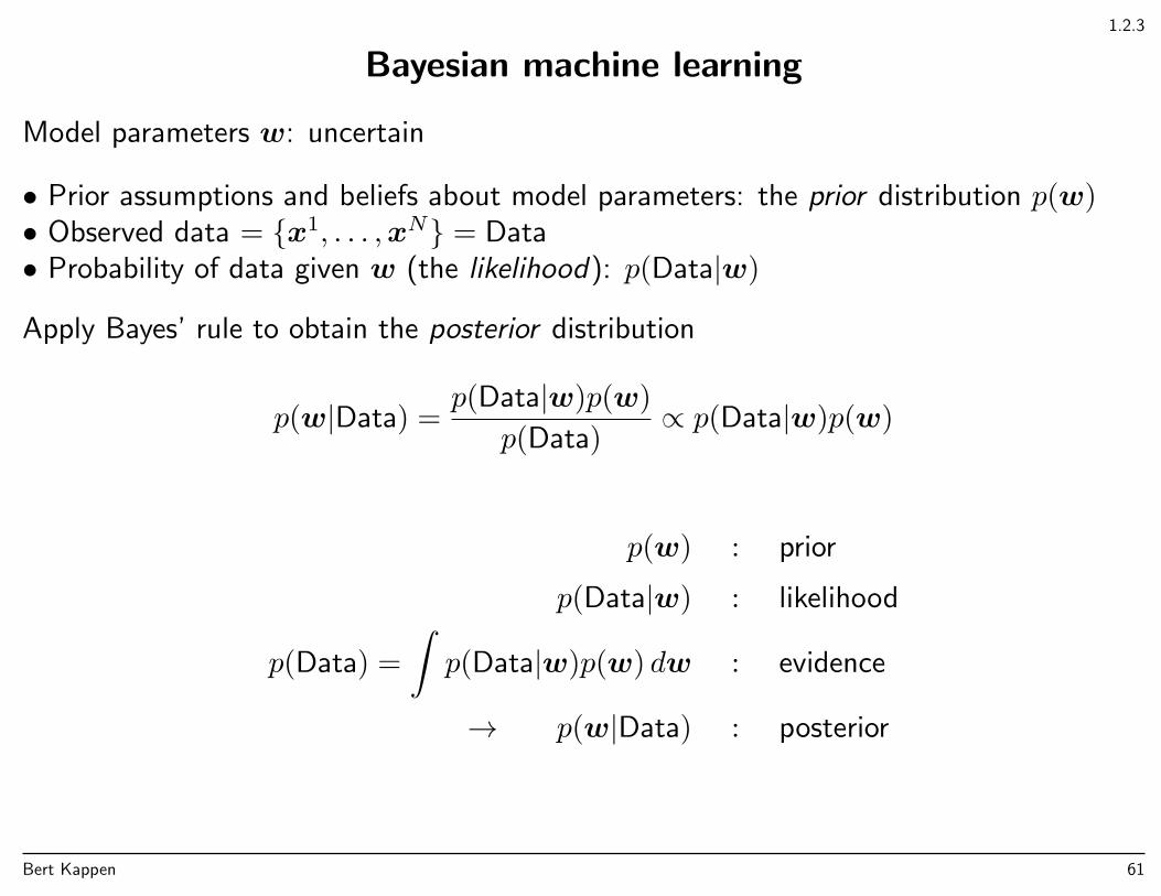
Bayesian machine learning
Model parameters w: uncertain
• Prior assumptions and beliefs about model parameters: the prior distribution p(w)• Observed data = x1, . . . ,xN = Data• Probability of data given w (the likelihood): p(Data|w)
Apply Bayes’ rule to obtain the posterior distribution
p(w|Data) =p(Data|w)p(w)
p(Data)∝ p(Data|w)p(w)
p(w) : prior
p(Data|w) : likelihood
p(Data) =
∫p(Data|w)p(w) dw : evidence
→ p(w|Data) : posterior
Bert Kappen 61
1.2.3
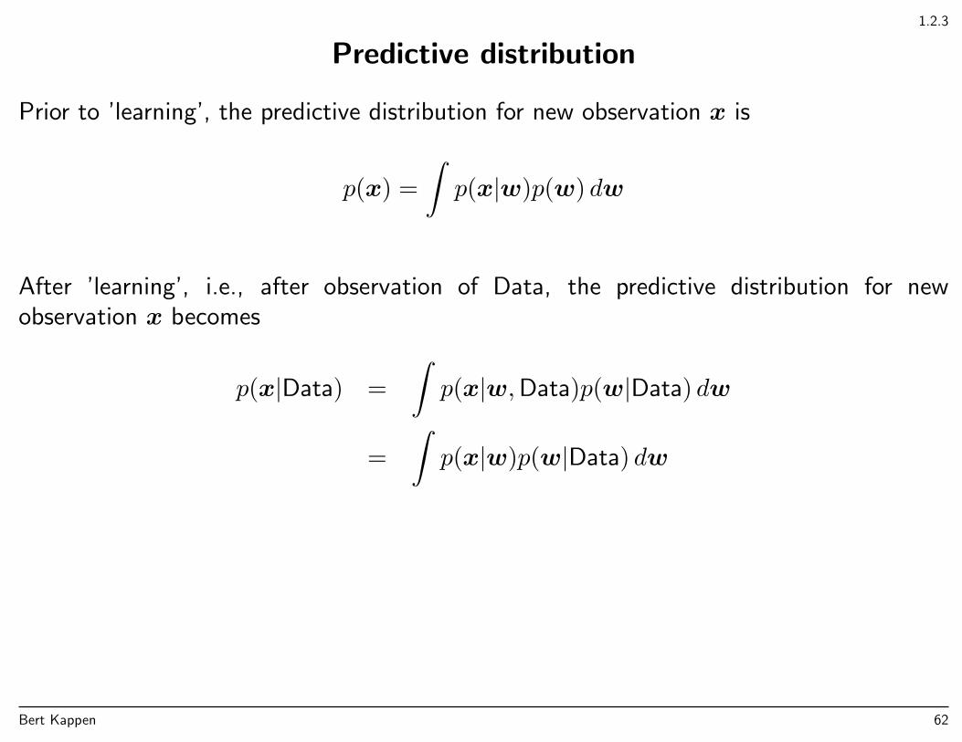
Predictive distribution
Prior to ’learning’, the predictive distribution for new observation x is
p(x) =
∫p(x|w)p(w) dw
After ’learning’, i.e., after observation of Data, the predictive distribution for newobservation x becomes
p(x|Data) =
∫p(x|w,Data)p(w|Data) dw
=
∫p(x|w)p(w|Data) dw
Bert Kappen 62
1.2.3
Bayesian vs frequentists view point
• Bayesians: there is a single fixed dataset (the one observed), and a probabilitydistribution of model parameters w which expresses a subjective belief includinguncertainty about the ‘true’ model parameters.
- They need a prior belief p(w), and apply Bayes rule to compute p(w|Data).
- Bayesians can talk about frequency that in repeated situations with this data w hasa certain value.
• Frequentists: there is a single (unknown) fixed model parameter vector w. Theyconsider the probability distribution of possible datasets p(Data|w) - although onlyone is actually observed.
- Frequentist can talk about frequency that estimators w in similar experiments, eachtime with different datasets drawn from p(Data|w), are within a certain confidenceinterval around the true w.
-They cannot make a claim for this particular data set. This is the price for not havinga ‘prior’.
Bert Kappen 63
additional example for 1.2.3
Toy example
Unknown binary prameter w = 0, 1Data is binary x = 0, 1, distributed according to P (x = w|w) = 0.9.
Given data x = 1 what can be said about w?
• Bayesian: needs a prior.
• Frequentist: estimator is w = x, so w = 1.
The frequentist provides a “confidence” that w is equal to w: In 90% of similarexperiments with outcomes x (either 0 or 1), the estimate w = x is correct. This is truesince P (x = w|w) = 0.9.
Bert Kappen 64
additional example for 1.2.3
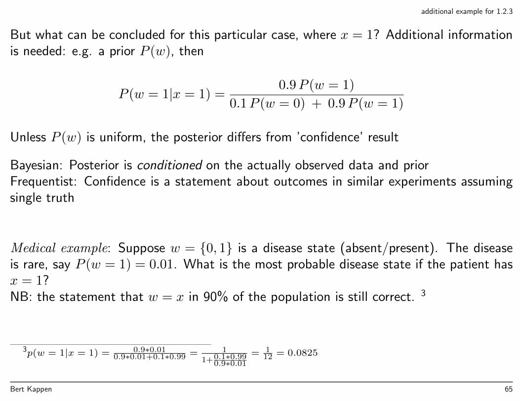
But what can be concluded for this particular case, where x = 1? Additional informationis needed: e.g. a prior P (w), then
P (w = 1|x = 1) =0.9P (w = 1)
0.1P (w = 0) + 0.9P (w = 1)
Unless P (w) is uniform, the posterior differs from ’confidence’ result
Bayesian: Posterior is conditioned on the actually observed data and priorFrequentist: Confidence is a statement about outcomes in similar experiments assumingsingle truth
Medical example: Suppose w = 0, 1 is a disease state (absent/present). The diseaseis rare, say P (w = 1) = 0.01. What is the most probable disease state if the patient hasx = 1?NB: the statement that w = x in 90% of the population is still correct. 3
3p(w = 1|x = 1) = 0.9∗0.010.9∗0.01+0.1∗0.99 = 1
1+0.1∗0.990.9∗0.01
= 112 = 0.0825
Bert Kappen 65
1.2.3
Bayesian vs frequentists
• Prior: inclusion of prior knowledge may be useful. True reflection of knowledge, orconvenient construct? Bad prior choice can overconfidently lead to poor result.
• Bayesian integrals cannot be calculated in general. Only approximate results possible,requiring intensive numerical computations.
• Frequentists methods of ‘resampling the data’, (crossvalidation, bootstrapping) areappealing
• Bayesian framework transparent and consistent. Assumptions are explicit, inference isa mechanstic procedure (Bayesian machinery) and results have a clear interpretation.
This course place emphasis on Bayesian approach. Frequentists maximum likelihoodmethod is viewed as an approximation.
Bert Kappen 66
1.2.4: p.24-25
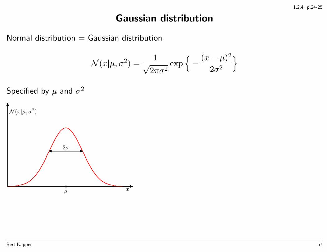
Gaussian distribution
Normal distribution = Gaussian distribution
N (x|µ, σ2) =1√
2πσ2exp
− (x− µ)2
2σ2
Specified by µ and σ2
N (x|µ, σ2)
x
2σ
µ
Bert Kappen 67
1.2.4: p.24-25
Gaussian is normalized, ∫ ∞−∞N (x|µ, σ2) dx = 1
The mean (= first moment), second moment, and variance are:
IE[x] = 〈x〉 =
∫ ∞−∞
xN (x|µ, σ2) dx = µ
⟨x2⟩
=
∫ ∞−∞
x2N (x|µ, σ2) dx = µ2 + σ2
var[x] =⟨x2⟩− 〈x〉2 = σ2
Bert Kappen 68
1.2.4: p.24-25
Multivariate Gaussian
In D dimensions
N (x|µ,Σ) =1
(2π)D/2|Σ|1/2 exp
(−1
2(x− µ)TΣ−1(x− µ)
)x,µ are D-dimensional vectors.
Σ is a D ×D covariance matrix, |Σ| is its determinant.
Bert Kappen 69
1.2.4: p.24-25
Mean vector and covariance matrix
IE[x] = 〈x〉 =
∫xN (x|µ,Σ) dx = µ
cov[x] =⟨(x− µ)(x− µ)T
⟩=
∫(x− µ)(x− µ)TN (x|µ,Σ) dx = Σ
We can also write this in component notation:
µi = 〈xi〉 =
∫xiN (x|µ,Σ) dx
Σij = 〈(xi − µi)(xj − µj)〉 =
∫(xi − µi)(xj − µj)N (x|µ,Σ) dx
N (x|µ,Σ) is specified by its mean and covariance, in total D(D+1)/2+D parameters.
Bert Kappen 70
1.2.4: p.26-28
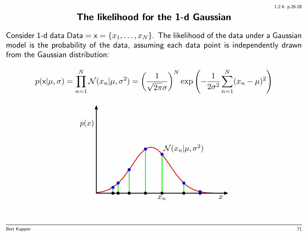
The likelihood for the 1-d Gaussian
Consider 1-d data Data = x = x1, . . . , xN. The likelihood of the data under a Gaussianmodel is the probability of the data, assuming each data point is independently drawnfrom the Gaussian distribution:
p(x|µ, σ) =
N∏n=1
N (xn|µ, σ2) =
(1√2πσ
)Nexp
(− 1
2σ2
N∑n=1
(xn − µ)2
)
x
p(x)
xn
N (xn|µ, σ2)
Bert Kappen 71
1.2.4: p.26-28
Maximum likelihood
Consider the log of the likelihood:
ln p(x|µ, σ) = − 1
2σ2
N∑n=1
(xn − µ)2 − N2
lnσ2 − N2
ln 2π
The values of µ and σ that maximize the likelihood are given by
µML =1
N
N∑n=1
xn σ2ML =
1
N
N∑n=1
(xn − µML)2
Bert Kappen 72
1.2.4: p.26-28
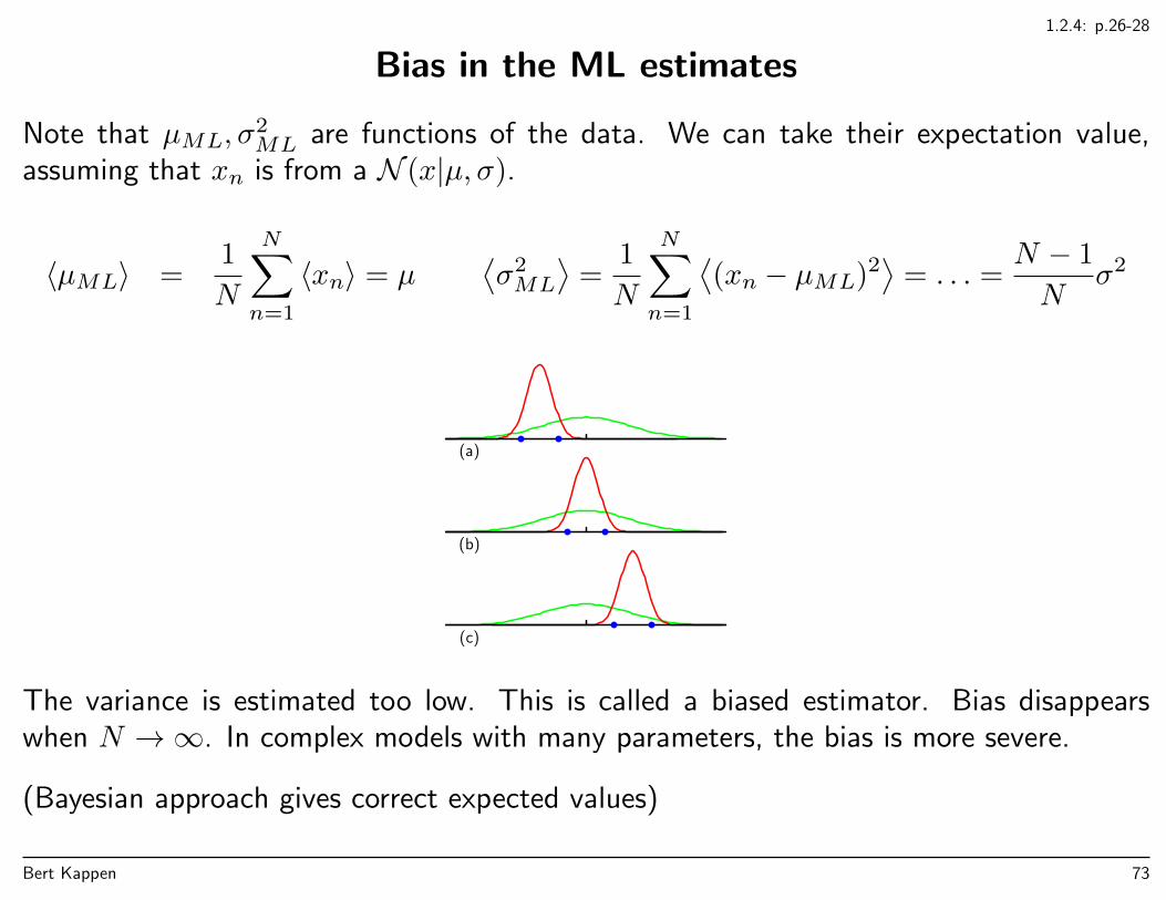
Bias in the ML estimates
Note that µML, σ2ML are functions of the data. We can take their expectation value,
assuming that xn is from a N (x|µ, σ).
〈µML〉 =1
N
N∑n=1
〈xn〉 = µ⟨σ2ML
⟩=
1
N
N∑n=1
⟨(xn − µML)2
⟩= . . . =
N − 1
Nσ2
(a)
(b)
(c)
The variance is estimated too low. This is called a biased estimator. Bias disappearswhen N →∞. In complex models with many parameters, the bias is more severe.
(Bayesian approach gives correct expected values)
Bert Kappen 73

1.2.5: p.28-29
Curve fitting re-visited
Now from a probabilistic perspective.
Target t is Gaussian distributed around mean y(x,w),
p(t|x,w, β) = N (t|y(x,w), β−1)
β = 1/σ2 is the precision.
t
xx0
2σy(x0,w)
y(x,w)
p(t|x0,w, β)
Bert Kappen 74
1.2.5: p.28-29
Curve fitting re-visited: ML
Training data: inputs x = (x1, . . . , xn), targets t = (t1, . . . , tn). (Assume β is known.)
Likelihood ,
p(t|x,w) =
N∏n=1
N (tn|y(xn,w), β−1)
Log-likelihood
ln p(t|x,w) = −β2
N∑n=1
(y(xn,w)− tn)2 + const(β)
With wML one can make predictions for a new input values x. The predictive distributionover the output t is:
p(t|x,wML) = N (t|y(x,wML), β−1)
Bert Kappen 75
1.2.5: p.30
Curve fitting re-visited MAP
Bayesian approach.Prior:
p(w|α) = N (w|α−1I) =( α
2π
)(M+1)/2
exp(−α
2wTw
)M is the dimension of w. Variables such as α, controling the distribution of parameters,are called ‘hyperparameters’.
Posterior using Bayes rule:
p(w|t, x, α, β) ∝ p(w|α)
N∏n=1
N (tn|y(xn,w), β−1)
− ln p(w|t, x, α, β) =β
2
N∑n=1
(y(xn,w)− tn)2 +α
2wTw + const(β)
Maximizing the posterior wrt w yields wMAP . Similar as Eq. 1.4. with λ = α/β
Bert Kappen 76
1.2.5: p.30
Bayesian curve fitting
Given the training data x, t we are not so much interested in w, but rather in theprediction of t for a new x: p(t|x, x, t). This is given by
p(t|x, x, t) =
∫dwp(t|x,w)p(w|x, t)
It is the average prediction of an ensemble of models p(t|x,w) parametrized by w andaveraged wrt to the posterior distribution p(w|x, t).
All quantities depend on α and β.
Bert Kappen 77

1.2.6
Bayesian curve fitting
Generalized linear model with ‘basis functions’ e.g., φi(x) = xi,
y(x,w) =∑i
φi(x)wi = φ(x)Tw
So: prediction given w is
p(t|x,w) = N (t|y(x,w), β−1) = N (t|φ(x)Tw, β−1)
The prior is Gaussian, the likelihood is a product of Gaussians. Thus the posterior isGaussian.
Bert Kappen 78
1.2.6
Result Bayesian curve fitting
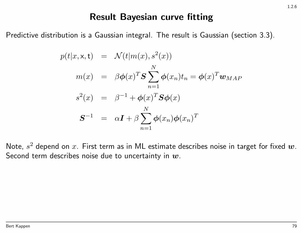
Predictive distribution is a Gaussian integral. The result is Gaussian (section 3.3).
p(t|x, x, t) = N (t|m(x), s2(x))
m(x) = βφ(x)TS
N∑n=1
φ(xn)tn = φ(x)TwMAP
s2(x) = β−1 + φ(x)TSφ(x)
S−1 = αI + β
N∑n=1
φ(xn)φ(xn)T
Note, s2 depend on x. First term as in ML estimate describes noise in target for fixed w.Second term describes noise due to uncertainty in w.
Bert Kappen 79
1.2.6
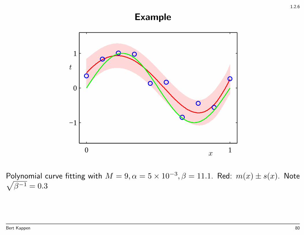
Example
x
t
0 1
−1
0
1
Polynomial curve fitting with M = 9, α = 5× 10⁻³, β = 11.1. Red: m(x)± s(x). Note√β−1 = 0.3
Bert Kappen 80

1.3
Model selection
Q: If we have different models to describe the data, which one should we choose?
Bert Kappen 81
1.3
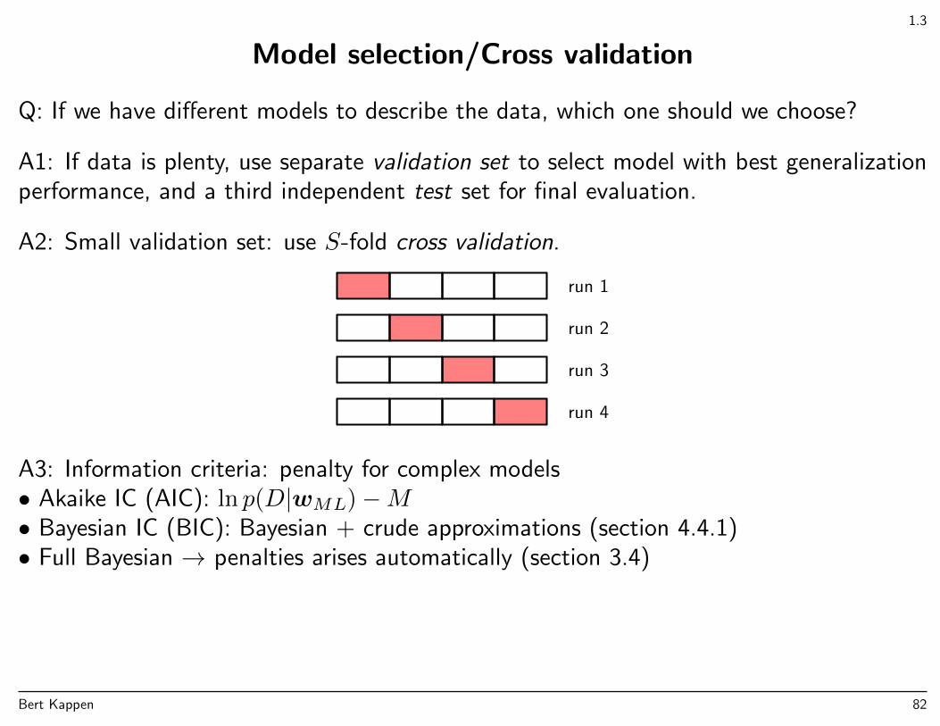
Model selection/Cross validation
Q: If we have different models to describe the data, which one should we choose?
A1: If data is plenty, use separate validation set to select model with best generalizationperformance, and a third independent test set for final evaluation.
A2: Small validation set: use S-fold cross validation.
run 1
run 2
run 3
run 4
A3: Information criteria: penalty for complex models• Akaike IC (AIC): ln p(D|wML)−M• Bayesian IC (BIC): Bayesian + crude approximations (section 4.4.1)• Full Bayesian → penalties arises automatically (section 3.4)
Bert Kappen 82
1.4: pp. 34–35
High-dimensional data/Binning
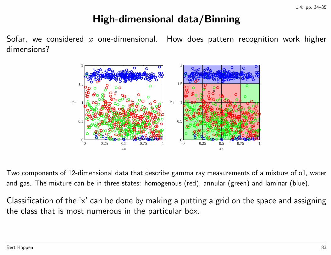
Sofar, we considered x one-dimensional. How does pattern recognition work higherdimensions?
x6
x7
0 0.25 0.5 0.75 10
0.5
1
1.5
2
x6
x7
0 0.25 0.5 0.75 10
0.5
1
1.5
2
Two components of 12-dimensional data that describe gamma ray measurements of a mixture of oil, water
and gas. The mixture can be in three states: homogenous (red), annular (green) and laminar (blue).
Classification of the ’x’ can be done by making a putting a grid on the space and assigningthe class that is most numerous in the particular box.
Bert Kappen 83
1.4: p. 35
High-dimensional data/Binning
Q: What is the disadvantage of this approach?
Bert Kappen 84

1.4: p. 35
Curse of dimensionality/Binning
Q: What is the disadvantage of this approach?A: This approach scales exponentially with dimensions.
x1
D = 1x1
x2
D = 2
x1
x2
x3
D = 3
In D dimensions: grid with length n consists of . . . hypercubes.
Bert Kappen 85
1.4: p. 35
Curse of dimensionality/Binning
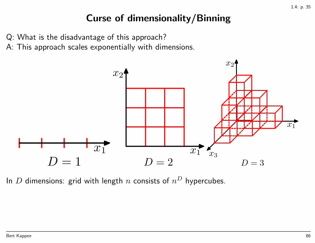
Q: What is the disadvantage of this approach?A: This approach scales exponentially with dimensions.
x1
D = 1x1
x2
D = 2
x1
x2
x3
D = 3
In D dimensions: grid with length n consists of nD hypercubes.
Bert Kappen 86
1.4: p. 36
Curse of dimensionality/Polynomials
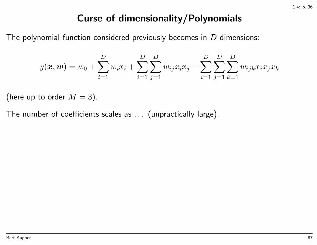
The polynomial function considered previously becomes in D dimensions:
y(x,w) = w0 +
D∑i=1
wixi +
D∑i=1
D∑j=1
wijxixj +
D∑i=1
D∑j=1
D∑k=1
wijkxixjxk
(here up to order M = 3).
The number of coefficients scales as . . . (unpractically large).
Bert Kappen 87

1.4: p. 36
Curse of dimensionality/Polynomials
The polynomial function considered previously becomes in D dimensions:
y(x,w) = w0 +
D∑i=1
wixi +
D∑i=1
D∑j=1
wijxixj +
D∑i=1
D∑j=1
D∑k=1
wijkxixjxk
(here up to order M = 3).
The number of coefficients scales as DM (unpractically large).
Bert Kappen 88
1.4: p. 37
Curse of dimensionality/Spheres
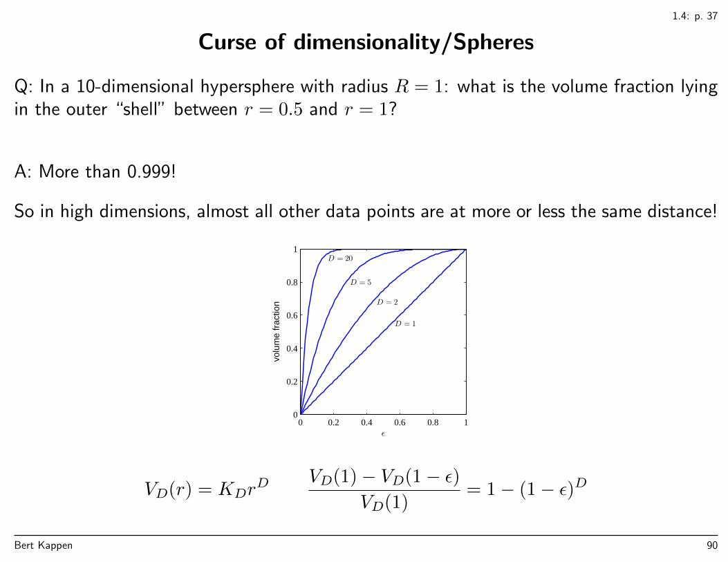
Q: In a 10-dimensional hypersphere with radius R = 1: what is the volume fraction lyingin the outer “shell” between r = 0.5 and r = 1?
Bert Kappen 89
1.4: p. 37
Curse of dimensionality/Spheres
Q: In a 10-dimensional hypersphere with radius R = 1: what is the volume fraction lyingin the outer “shell” between r = 0.5 and r = 1?
A: More than 0.999!
So in high dimensions, almost all other data points are at more or less the same distance!
ε
volu
me
frac
tion
D = 1
D = 2
D = 5
D = 20
0 0.2 0.4 0.6 0.8 10
0.2
0.4
0.6
0.8
1
VD(r) = KDrD VD(1)− VD(1− ε)
VD(1)= 1− (1− ε)D
Bert Kappen 90

1.4: p. 37
Spheres in high dimension have most of their volume on the boundary.
Bert Kappen 91
1.4: p. 37
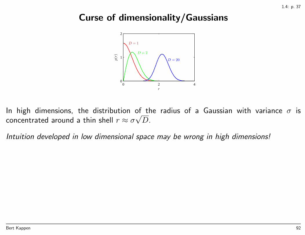
Curse of dimensionality/Gaussians
D = 1
D = 2
D = 20
r
p(r)
0 2 40
1
2
In high dimensions, the distribution of the radius of a Gaussian with variance σ isconcentrated around a thin shell r ≈ σ
√D.
Intuition developed in low dimensional space may be wrong in high dimensions!
Bert Kappen 92
1.4: p. 38
Curse of dimensionality
Is machine learning even possible in high dimensions?
• Data often in low dimensional subspace: only a few dimensions are relevant.
– Object located in 3-D→ images of objects are N -D→ there should be 3-D manifold(curved subspace)
• Smoothness, local interpolation (note: this is also needed in low dimensions).
Bert Kappen 93

1.5
Decision theory
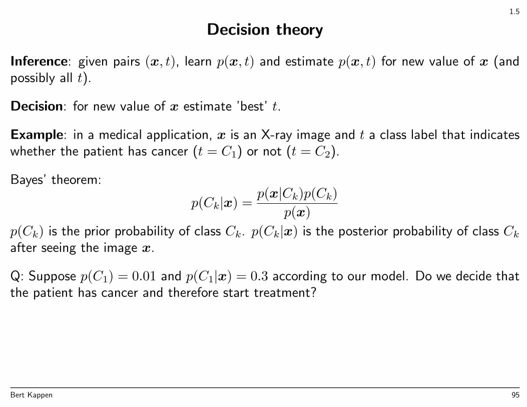
Inference: given pairs (x, t), learn p(x, t) and estimate p(x, t) for new value of x (andpossibly all t).
Decision: for new value of x estimate ’best’ t.
Example: in a medical application, x is an X-ray image and t a class label that indicateswhether the patient has cancer (t = C1) or not (t = C2).
Bert Kappen 94
1.5
Decision theory
Inference: given pairs (x, t), learn p(x, t) and estimate p(x, t) for new value of x (andpossibly all t).
Decision: for new value of x estimate ’best’ t.
Example: in a medical application, x is an X-ray image and t a class label that indicateswhether the patient has cancer (t = C1) or not (t = C2).
Bayes’ theorem:
p(Ck|x) =p(x|Ck)p(Ck)
p(x)
p(Ck) is the prior probability of class Ck. p(Ck|x) is the posterior probability of class Ckafter seeing the image x.
Q: Suppose p(C1) = 0.01 and p(C1|x) = 0.3 according to our model. Do we decide thatthe patient has cancer and therefore start treatment?
Bert Kappen 95
1.5.1
Decision theory
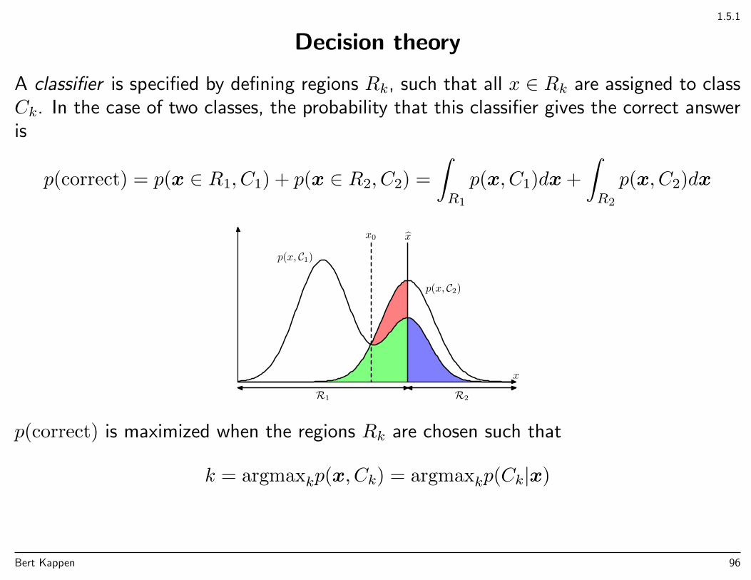
A classifier is specified by defining regions Rk, such that all x ∈ Rk are assigned to classCk. In the case of two classes, the probability that this classifier gives the correct answeris
p(correct) = p(x ∈ R1, C1) + p(x ∈ R2, C2) =
∫R1
p(x, C1)dx+
∫R2
p(x, C2)dx
R1 R2
x0 x
p(x, C1)
p(x, C2)
x
p(correct) is maximized when the regions Rk are chosen such that
k = argmaxkp(x, Ck) = argmaxkp(Ck|x)
Bert Kappen 96

1.5.1
Decision theory/Example
Example: in a medical application, x is an X-ray image and t a class label that indicateswhether the patient has cancer (t = C1) or not (t = C2).
Q: Suppose p(C1) = 0.01 and p(C1|x) = 0.3 according to our model. Do we decide thatthe patient has cancer and therefore start treatment?
Bert Kappen 97

1.5.1
Decision theory/Example
Example: in a medical application, x is an X-ray image and t a class label that indicateswhether the patient has cancer (t = C1) or not (t = C2).
Q: Suppose p(C1) = 0.01 and p(C1|x) = 0.3 according to our model. Do we decide thatthe patient has cancer and therefore start treatment?
A: If we want to maximize the chance of making the correct decision, we have to pick ksuch that p(Ck|x) is maximal.Because p(C1|x) = 0.3 and p(C2|x) = 0.7, the answer is no: we decide that the patientdoes not have cancer.
Bert Kappen 98
1.5.2
Decision theory/Expected loss
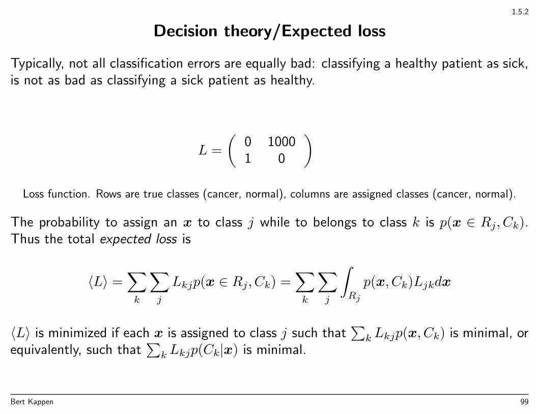
Typically, not all classification errors are equally bad: classifying a healthy patient as sick,is not as bad as classifying a sick patient as healthy.
L =
(0 10001 0
)Loss function. Rows are true classes (cancer, normal), columns are assigned classes (cancer, normal).
The probability to assign an x to class j while to belongs to class k is p(x ∈ Rj, Ck).Thus the total expected loss is
〈L〉 =∑k
∑j
Lkjp(x ∈ Rj, Ck) =∑k
∑j
∫Rj
p(x, Ck)Ljkdx
〈L〉 is minimized if each x is assigned to class j such that∑k Lkjp(x, Ck) is minimal, or
equivalently, such that∑k Lkjp(Ck|x) is minimal.
Bert Kappen 99
1.5.2
Decision theory/Example
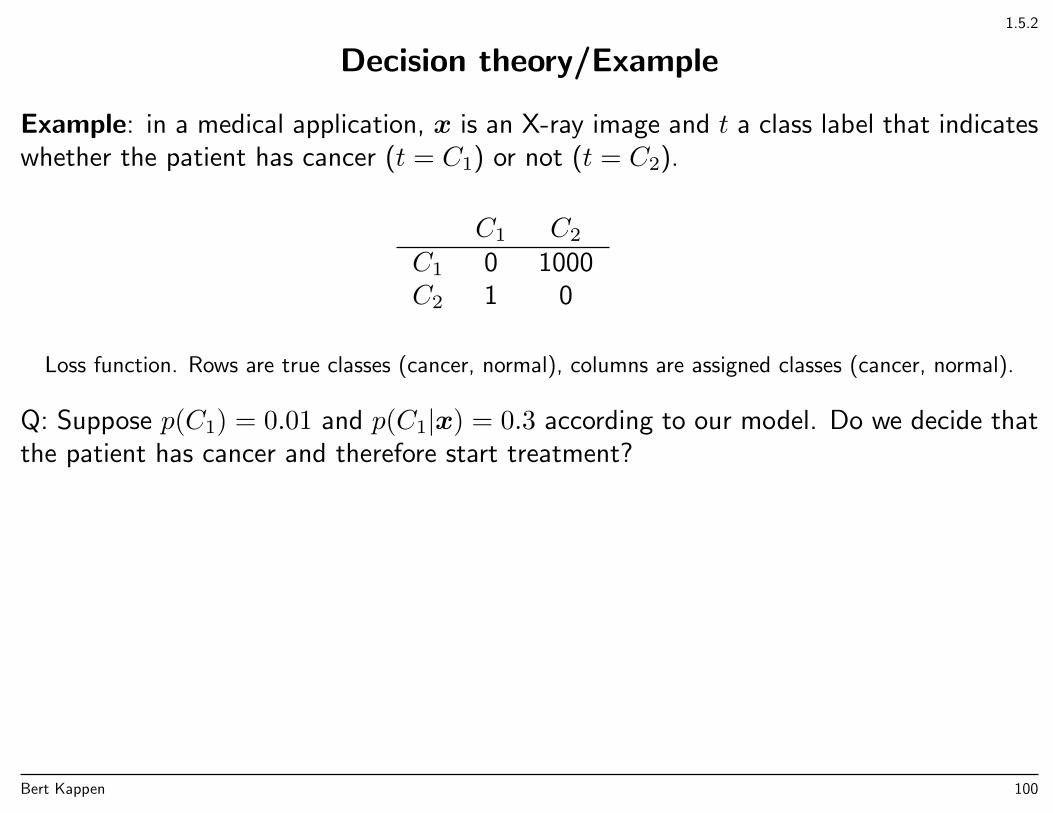
Example: in a medical application, x is an X-ray image and t a class label that indicateswhether the patient has cancer (t = C1) or not (t = C2).
C1 C2
C1 0 1000C2 1 0
Loss function. Rows are true classes (cancer, normal), columns are assigned classes (cancer, normal).
Q: Suppose p(C1) = 0.01 and p(C1|x) = 0.3 according to our model. Do we decide thatthe patient has cancer and therefore start treatment?
Bert Kappen 100
1.5.2
Decision theory/Example
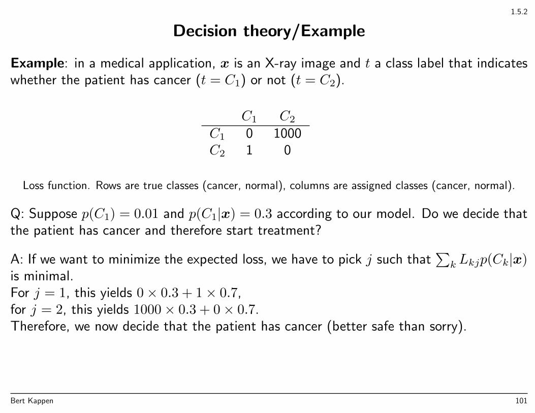
Example: in a medical application, x is an X-ray image and t a class label that indicateswhether the patient has cancer (t = C1) or not (t = C2).
C1 C2
C1 0 1000C2 1 0
Loss function. Rows are true classes (cancer, normal), columns are assigned classes (cancer, normal).
Q: Suppose p(C1) = 0.01 and p(C1|x) = 0.3 according to our model. Do we decide thatthe patient has cancer and therefore start treatment?
A: If we want to minimize the expected loss, we have to pick j such that∑k Lkjp(Ck|x)
is minimal.For j = 1, this yields 0× 0.3 + 1× 0.7,for j = 2, this yields 1000× 0.3 + 0× 0.7.Therefore, we now decide that the patient has cancer (better safe than sorry).
Bert Kappen 101
1.5.3
Decision theory/Reject option
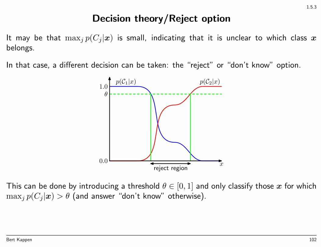
It may be that maxj p(Cj|x) is small, indicating that it is unclear to which class xbelongs.
In that case, a different decision can be taken: the “reject” or “don’t know” option.
x
p(C1|x) p(C2|x)
0.0
1.0θ
reject region
This can be done by introducing a threshold θ ∈ [0, 1] and only classify those x for whichmaxj p(Cj|x) > θ (and answer “don’t know” otherwise).
Bert Kappen 102
1.5.4
Decision theory/Discriminant functions
Instead of first learning a probability model and then making a decision, one can alsodirectly learn a decision rule (a classifier) without the intermediate step of a probabilitymodel.
A set of approaches:
• Learn a model for the class conditional probabilities p(x|Ck). Use Bayes’ rule tocompute p(Ck|x) and construct a classifier using decision theory. This approach is themost complex (section 4.2).
• Learn the inference problem p(Ck|x) directly and construct a classifier using decisiontheory. This approach is simpler, since no input model p(x) is learned (see figure)(section 4.3)
• Learn f(x), called a discriminant function, that maps x directly onto a class label0, 1, 2, . . .. Even simpler, only decision boundary is learned. But information on theexpected classification error is lost (section 4.1, not treated).
Bert Kappen 103
1.5.4
Decision theory/Discriminant functions
p(x|C1)
p(x|C2)
x
clas
s de
nsiti
es
0 0.2 0.4 0.6 0.8 10
1
2
3
4
5
x
p(C1|x) p(C2|x)
0 0.2 0.4 0.6 0.8 10
0.2
0.4
0.6
0.8
1
1.2
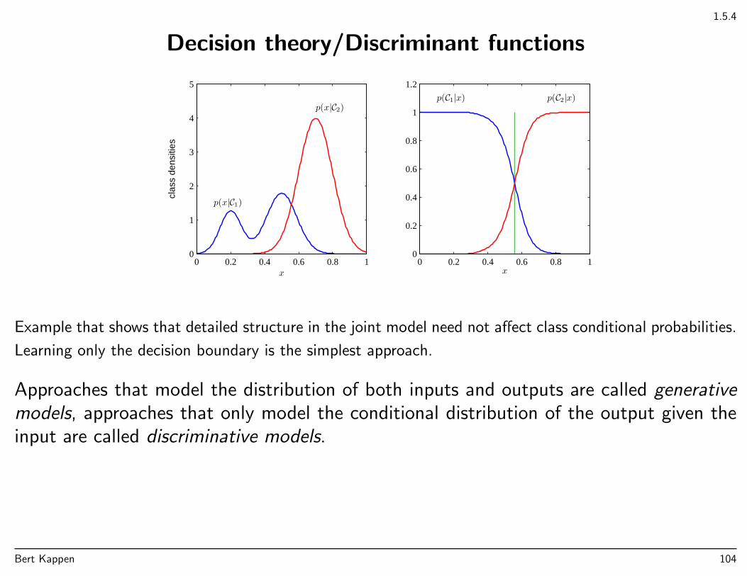
Example that shows that detailed structure in the joint model need not affect class conditional probabilities.
Learning only the decision boundary is the simplest approach.
Approaches that model the distribution of both inputs and outputs are called generativemodels, approaches that only model the conditional distribution of the output given theinput are called discriminative models.
Bert Kappen 104
1.5.4
Decision theory/Discriminant functions
Advantages of generative probability model instead of discriminant function:
Minimizing risk The loss matrix may change over time whereas the class probabilitiesmay not (for instance, in a financial application).
Reject option p(x) can be used to reject unlikely inputs x by p(x) =∑k p(x|Ck)p(Ck)
Unbalanced data One can compensate for unbalanced data sets. For instance, in thecancer example, there may be 1000 times more healthy patients than cancer patients.Very good classification (99.9 % correct) is obtained by classifying everyone as healthy.Using the posterior probability one can compute p(Ck = cancer|x). Although thisprobability may be low, it may be significantly higher than p(Ck = cancer), indicatinga risk of cancer.
Bert Kappen 105
1.5.5
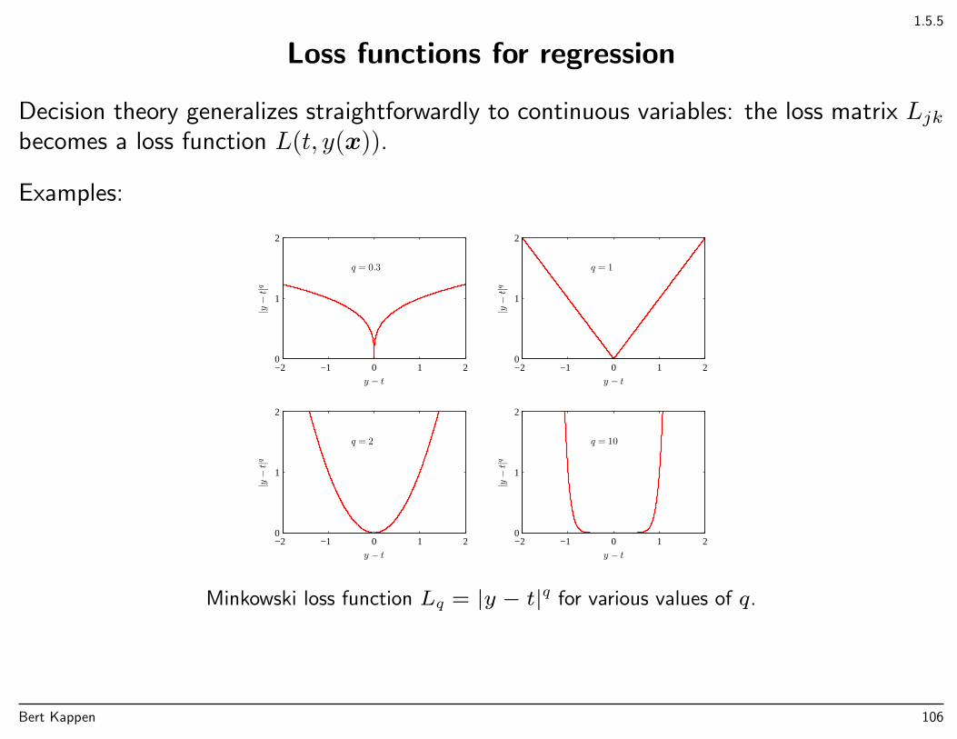
Loss functions for regression
Decision theory generalizes straightforwardly to continuous variables: the loss matrix Ljkbecomes a loss function L(t, y(x)).
Examples:
y − t
|y−t|q
q = 0.3
−2 −1 0 1 20
1
2
y − t
|y−t|q
q = 1
−2 −1 0 1 20
1
2
y − t
|y−t|q
q = 2
−2 −1 0 1 20
1
2
y − t
|y−t|q
q = 10
−2 −1 0 1 20
1
2
Minkowski loss function Lq = |y − t|q for various values of q.
Bert Kappen 106
1.5.5
Loss functions for regression/Quadratic loss
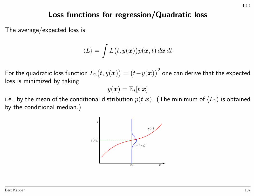
The average/expected loss is:
〈L〉 =
∫L(t, y(x)
)p(x, t) dx dt
For the quadratic loss function L2
(t, y(x)
)=(t−y(x)
)2one can derive that the expected
loss is minimized by takingy(x) = Et[t|x]
i.e., by the mean of the conditional distribution p(t|x). (The minimum of 〈L1〉 is obtainedby the conditional median.)
t
xx0
y(x0)
y(x)
p(t|x0)
Bert Kappen 107
1.6: pp. 48–49
Information theory
Information is a measure of the ’degree of surprise’ that a certain value gives us.Unlikely events are informative, likely events less so. Certain events give us no additionalinformation. Thus, information decreases with the probability of the event.
Let us denote h(x) the information of x. Then if x, y are two independent events:h(x, y) = h(x) + h(y). Since p(x, y) = p(x)p(y) we see that
h(x) = − log2 p(x)
is a good candidate to quantify the information in x.
If x is observed repeatedly then the expected information is
H[x] := 〈− log2 p〉 = −∑x
p(x) log2 p(x)
is the entropy of the distribution p.
Bert Kappen 108
1.6: p. 50
Information theory
Example 1: x can have 8 values with equal probability, then H(x) = −8 × 18 log 1
8 = 3bits.
Example 2: x can have 8 values with probabilities (12,
14,
18,
116,
164,
164,
164,
164). Then
H(x) = −1
2log
1
2− 1
4log
1
4− 1
8log
1
8− 1
16log
1
16− 4
64log
1
64= 2bits
which is smaller than for the uniform distribution.
Noiseless coding theorem: Entropy is a lower bound on the average number of bits neededto transmit a random variable (Shannon 1948).
Q: How can we transmit x in example 2 most efficiently?
Bert Kappen 109
1.6: p. 50
Information theory
Example 1: x can have 8 values with equal probability, then H(x) = −8 × 18 log 1
8 = 3bits.
Example 2: x can have 8 values with probabilities (12,
14,
18,
116,
164,
164,
164,
164). Then
H(x) = −1
2log
1
2− 1
4log
1
4− 1
8log
1
8− 1
16log
1
16− 4
64log
1
64= 2bits
which is smaller than for the uniform distribution.
Noiseless coding theorem: Entropy is a lower bound on the average number of bits neededto transmit a random variable (Shannon 1948).
A: We can encode x as a 3 bit binary number, in which case the expected code length is3 bits. We can do better, by coding likely x smaller and unlikely x larger, for instance 0,10, 110, 1110, 111100, 111101, 111110, 111111. Then
Av.codelength =1
2× 1 +
1
4× 2 +
1
8× 3 +
1
16× 4 +
4
64× 6 = 2bits
Bert Kappen 110
1.6: p. 52
Information theory
prob
abili
ties
H = 1.77
0
0.25
0.5
prob
abili
ties
H = 3.09
0
0.25
0.5
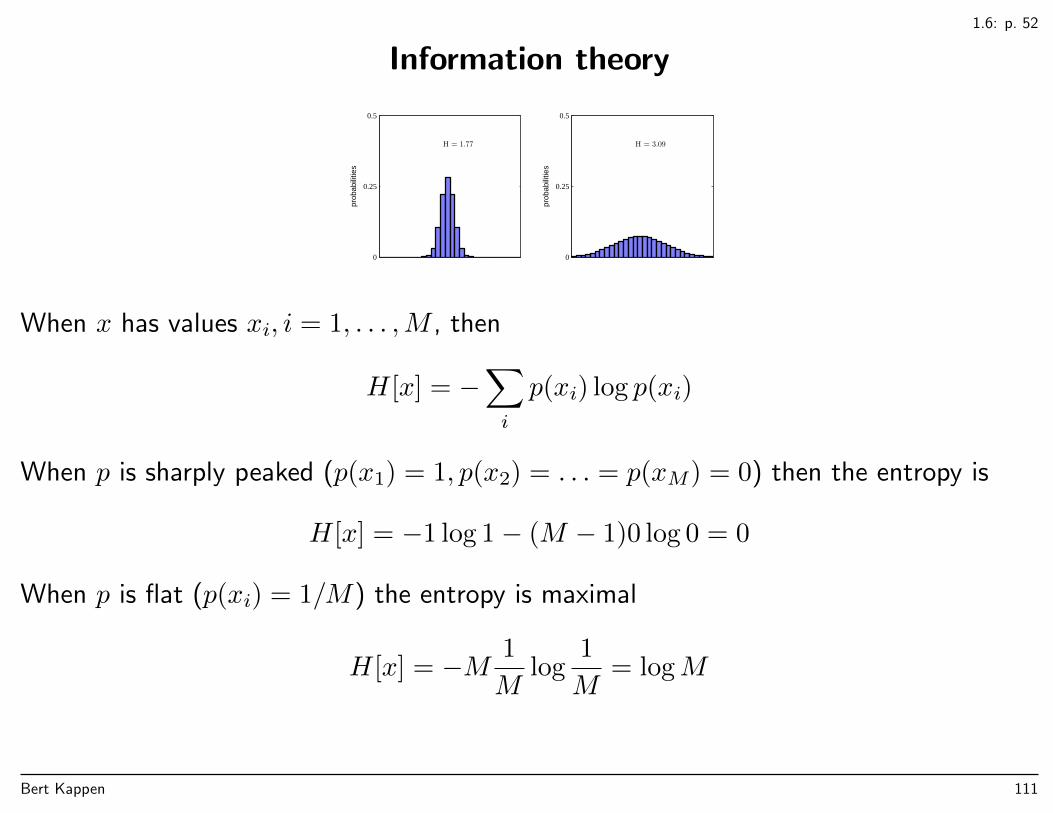
When x has values xi, i = 1, . . . ,M , then
H[x] = −∑i
p(xi) log p(xi)
When p is sharply peaked (p(x1) = 1, p(x2) = . . . = p(xM) = 0) then the entropy is
H[x] = −1 log 1− (M − 1)0 log 0 = 0
When p is flat (p(xi) = 1/M) the entropy is maximal
H[x] = −M 1
Mlog
1
M= logM
Bert Kappen 111
1.6: pp. 53–54
Information theory/Maximum entropy
For p(x) a distribution density over a continuous value x we define the (differential)entropy as
H[x] = −∫p(x) log p(x)dx
Suppose that all we know about p is its mean µ and its variance σ2.
Q: What is the distribution p with mean µ and variance σ2 that is as uninformative aspossible, i.e., which maximizes the entropy?
Bert Kappen 112
1.6: pp. 53–54
Information theory/Maximum entropy
For p(x) a distribution density over a continuous value x we define the (differential)entropy as
H[x] = −∫p(x) log p(x)dx
Suppose that all we know about p is its mean µ and its variance σ2.
Q: What is the distribution p with mean µ and variance σ2 that is as uninformative aspossible, i.e., which maximizes the entropy?
A: The Gaussian distribution N (x|µ, σ2) (exercise 1.34 and 1.35).
Bert Kappen 113
1.6.1
Information theory/KL-divergence
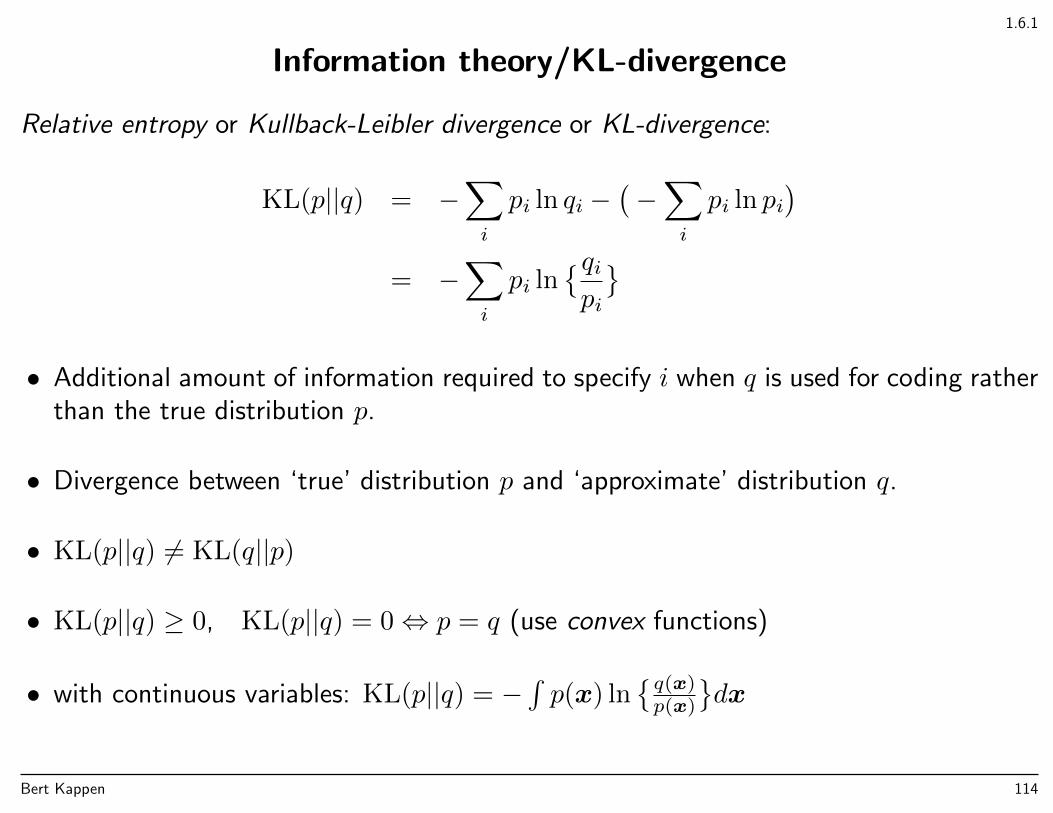
Relative entropy or Kullback-Leibler divergence or KL-divergence:
KL(p||q) = −∑i
pi ln qi −(−∑i
pi ln pi)
= −∑i
pi lnqipi
• Additional amount of information required to specify i when q is used for coding rather
than the true distribution p.
• Divergence between ‘true’ distribution p and ‘approximate’ distribution q.
• KL(p||q) 6= KL(q||p)
• KL(p||q) ≥ 0, KL(p||q) = 0⇔ p = q (use convex functions)
• with continuous variables: KL(p||q) = −∫p(x) ln
q(x)p(x)
dx
Bert Kappen 114
1.6.1: p. 56
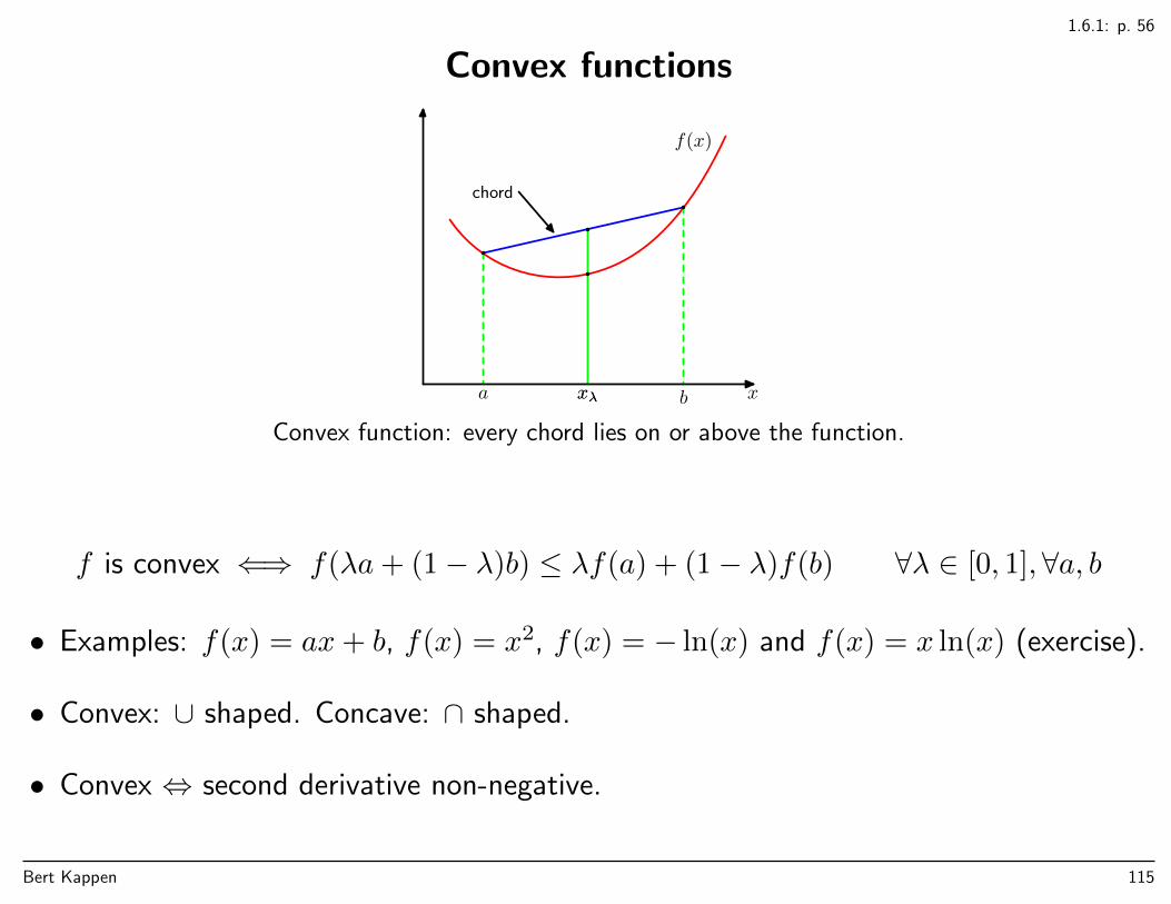
Convex functions
xa bxλ
chord
xλ
f(x)
Convex function: every chord lies on or above the function.
f is convex ⇐⇒ f(λa+ (1− λ)b) ≤ λf(a) + (1− λ)f(b) ∀λ ∈ [0, 1],∀a, b
• Examples: f(x) = ax+ b, f(x) = x2, f(x) = − ln(x) and f(x) = x ln(x) (exercise).
• Convex: ∪ shaped. Concave: ∩ shaped.
• Convex ⇔ second derivative non-negative.
Bert Kappen 115
1.6.1: p. 56
Convex functions/Jensen’s inequality
Convex functions satisfy Jensen’s inequality
f
(M∑i=1
λixi
)≤
M∑i=1
λif(xi)
where λi ≥ 0,∑i λi = 1, for any set points xi.
In other words:f(〈x〉) ≤ 〈f(x)〉
Example: to show that KL(p||q), we apply Jensen’s inequality with λi = pi, making useof the fact that − ln(x) is convex:
KL(p||q) = −∑i
pi ln
(qipi
)≥ − ln
(∑i
piqipi
)= − ln
(∑i
qi
)= 0
Bert Kappen 116
1.6.1: p. 57
Information theory and density estimation
Relation with maximum likelihood:
Empirical distribution :
p(x) =1
N
N∑n=1
δ(x− xn)
Approximating distribution (model) : q(x|θ)
KL(p||q) = −∫p(x) ln q(x|θ)dx−
∫p(x) ln p(x)dx
= − 1
N
N∑n=1
ln q(xn|θ) + const.
Thus, minimizing the KL-divergence between the empirical distribution p(x) and themodel distribution q(x|θ) is equivalent to maximum likelihood (i.e., maximizing thelikelihood of i.i.d. data with respect to the the model parameters θ).
Bert Kappen 117
1.6.1: pp. 57–58
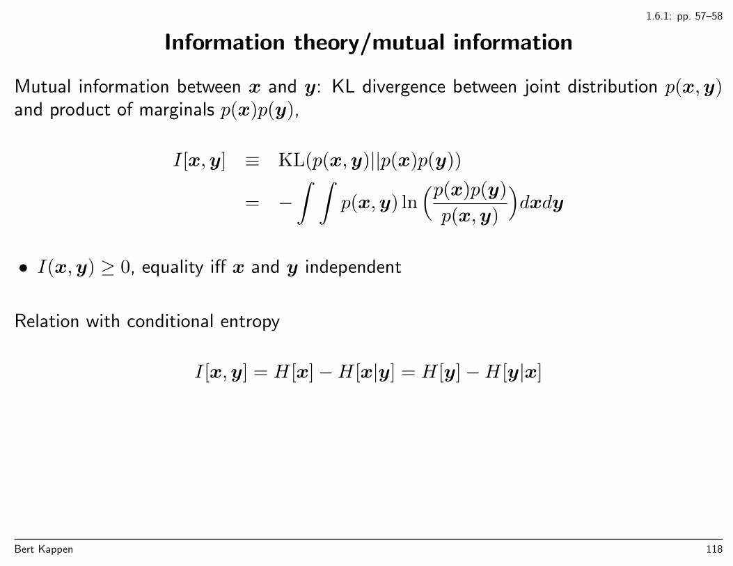
Information theory/mutual information
Mutual information between x and y: KL divergence between joint distribution p(x,y)and product of marginals p(x)p(y),
I[x,y] ≡ KL(p(x,y)||p(x)p(y))
= −∫ ∫
p(x,y) ln(p(x)p(y)
p(x,y)
)dxdy
• I(x,y) ≥ 0, equality iff x and y independent
Relation with conditional entropy
I[x,y] = H[x]−H[x|y] = H[y]−H[y|x]
Bert Kappen 118
Appendix E
Lagrange multipliers
Minimize f(x) under constraint: g(x) = 0.
Fancy formulation: define Lagrangian,
L(x, λ) = f(x) + λg(x)
λ is called a Lagrange multiplier.
The constraint minimization of f w.r.t x equivalent to unconstraint minimization ofmaxλL(x, λ) w.r.t x. The maximization w.r.t to λ yields the following function of x
maxλ
L(x, λ) = f(x) if g(x) = 0
maxλ
L(x, λ) =∞ otherwise
Bert Kappen 119
Appendix E
Lagrange multipliers
Under certain conditions, in particular f(x) convex (i.e. the matrix of second derivativespositive definite) and g(x) linear,
minx
maxλ
L(x, λ) = maxλ
minxL(x, λ)
Procedure:
1. Minimize L(x, λ) w.r.t x, e.g. by taking the gradient and set to zero. This yields a(parametrized) solution x(λ).
2. Maximize L(x(λ), λ) w.r.t. λ. The solution λ∗ is precisely such that g(x(λ∗)) = 0.
3. The solution of the constraint optimization problem is
x∗ = x(λ∗)
Bert Kappen 120
Appendix E
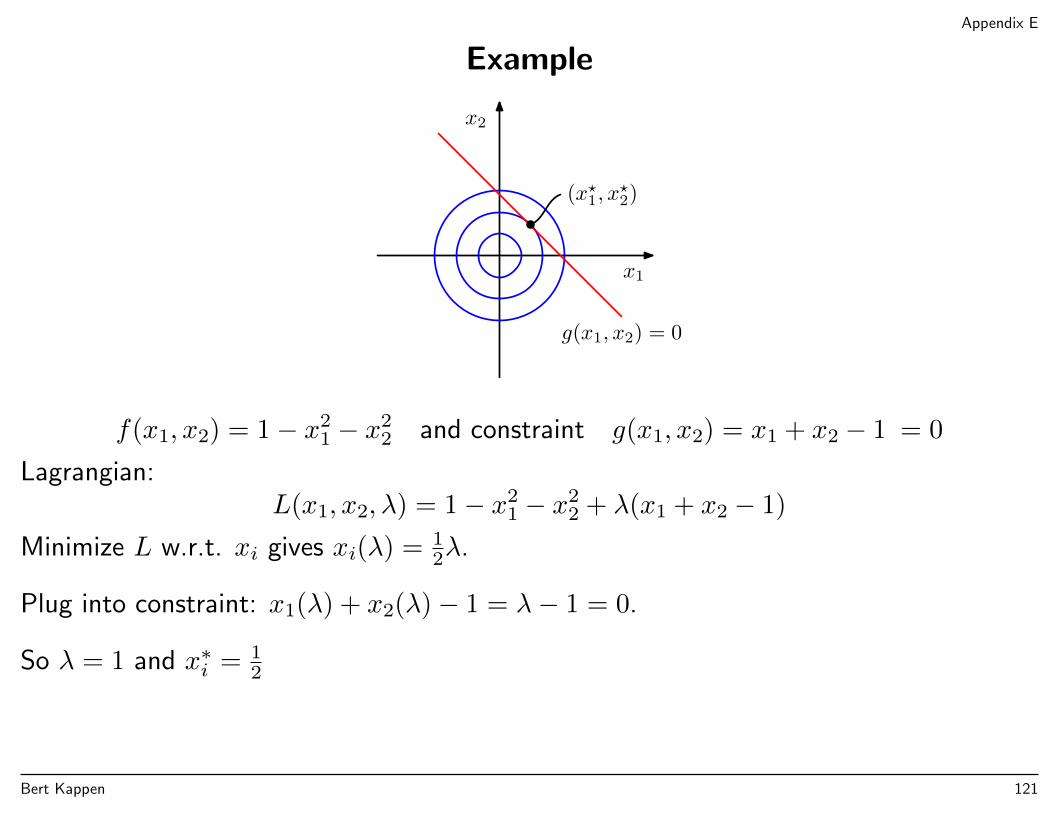
Example
g(x1, x2) = 0
x1
x2
(x?1, x
?2)
f(x1, x2) = 1− x21 − x2
2 and constraint g(x1, x2) = x1 + x2 − 1 = 0
Lagrangian:L(x1, x2, λ) = 1− x2
1 − x22 + λ(x1 + x2 − 1)
Minimize L w.r.t. xi gives xi(λ) = 12λ.
Plug into constraint: x1(λ) + x2(λ)− 1 = λ− 1 = 0.
So λ = 1 and x∗i = 12
Bert Kappen 121
Appendix E
Some remarks
• Works as well for maximization (of concave functions) under constraints. Theprocedure is essentially the same.
• The sign in front of the λ can be chosen as you want:
L(x, λ) = f(x) + λg(x) or L(x, λ) = f(x)− λg(x)
work equally well.
• More constraints? For each constraint gi(x) = 0 a Lagrange multiplier λi, so
L(x, λ) = f(x) +∑i
λigi(x)
• Similar methods apply for inequality constraints g(x) ≥ 0 (restricts λ).
Bert Kappen 122
2
Chapter 2
Probability distributions
• Density estimation
• Parametric distributions
• Maximum likelihood, Bayesian inference, conjugate priors
• Bernoulli (binary), Beta, Gaussian, ..., exponential family
• Nonparametric distribution
Bert Kappen 123
2.1
Binary variables / Bernoulli distribution
x ∈ 0, 1
p(x = 1|µ) = µ,
p(x = 0|µ) = 1− µ
Bernoulli distribution:Bern(x|µ) = µx(1− µ)1−x
Mean and variance:
IE[x] = µ
var[x] = µ(1− µ)
Bert Kappen 124
2.1
Binary variables / Bernoulli distribution
Data set (i.i.d) D = x1, . . . , xn, with xi ∈ 0, 1.
Likelihood:p(D|µ) =
∏n
p(xn|µ) =∏n
µxn(1− µ)1−xn
Log likelihood
ln p(D|µ) =∑n
ln p(xn|µ) =∑n
xn lnµ+ (1− xn) ln(1− µ)
= m lnµ+ (N −m) ln(1− µ)
where m =∑n xn, the total number of xn = 1.
Maximization w.r.t µ gives maximum likelihood solution:
µML =m
N
Bert Kappen 125
2.1.1
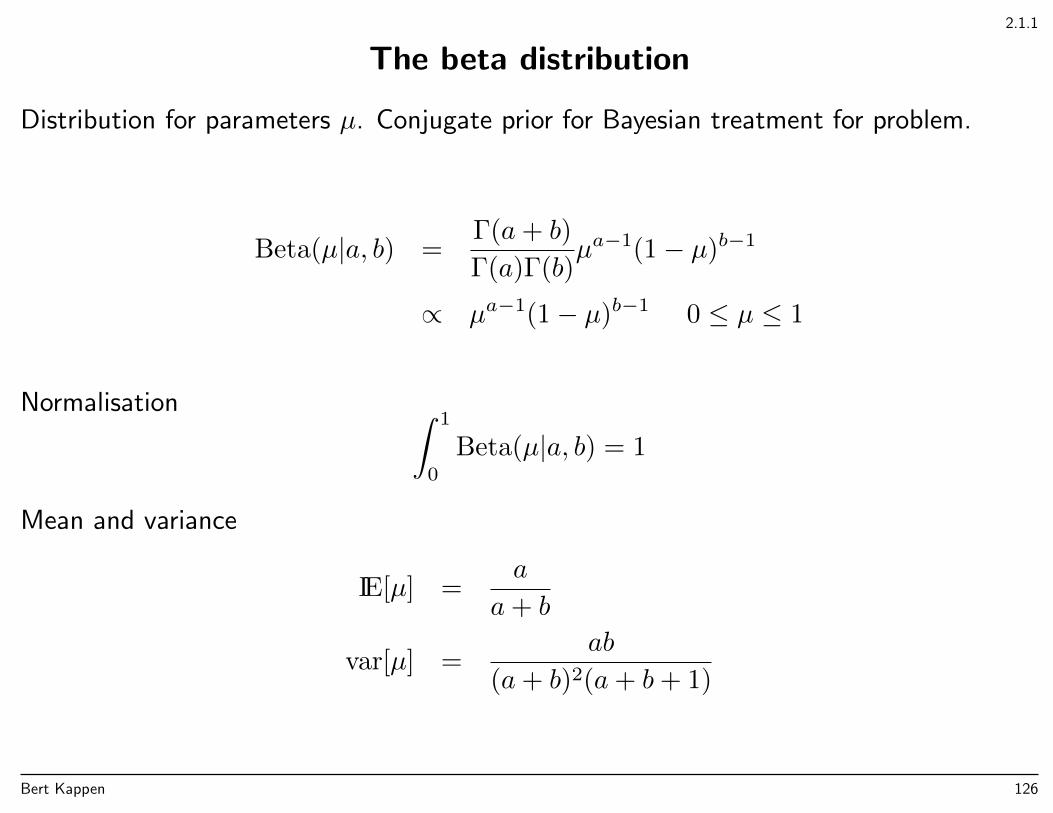
The beta distribution
Distribution for parameters µ. Conjugate prior for Bayesian treatment for problem.
Beta(µ|a, b) =Γ(a+ b)
Γ(a)Γ(b)µa−1(1− µ)b−1
∝ µa−1(1− µ)b−1 0 ≤ µ ≤ 1
Normalisation ∫ 1
0
Beta(µ|a, b) = 1
Mean and variance
IE[µ] =a
a+ b
var[µ] =ab
(a+ b)2(a+ b+ 1)
Bert Kappen 126
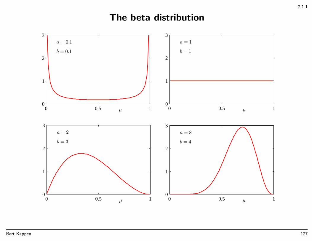
2.1.1
The beta distribution
µ
a = 0.1
b = 0.1
0 0.5 10
1
2
3
µ
a = 1
b = 1
0 0.5 10
1
2
3
µ
a = 2
b = 3
0 0.5 10
1
2
3
µ
a = 8
b = 4
0 0.5 10
1
2
3
Bert Kappen 127
2.1.1
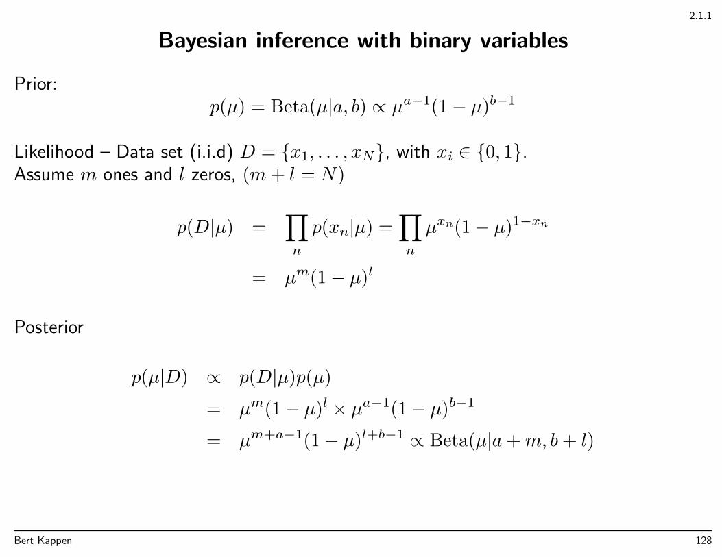
Bayesian inference with binary variables
Prior:p(µ) = Beta(µ|a, b) ∝ µa−1(1− µ)b−1
Likelihood – Data set (i.i.d) D = x1, . . . , xN, with xi ∈ 0, 1.Assume m ones and l zeros, (m+ l = N)
p(D|µ) =∏n
p(xn|µ) =∏n
µxn(1− µ)1−xn
= µm(1− µ)l
Posterior
p(µ|D) ∝ p(D|µ)p(µ)
= µm(1− µ)l × µa−1(1− µ)b−1
= µm+a−1(1− µ)l+b−1 ∝ Beta(µ|a+m, b+ l)
Bert Kappen 128
2.1.1
Bayesian inference with binary variables
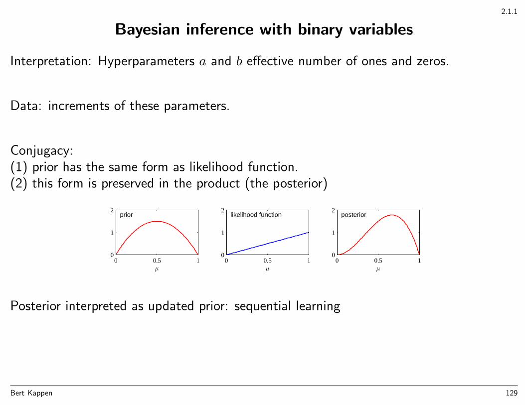
Interpretation: Hyperparameters a and b effective number of ones and zeros.
Data: increments of these parameters.
Conjugacy:(1) prior has the same form as likelihood function.(2) this form is preserved in the product (the posterior)
µ
prior
0 0.5 10
1
2
µ
likelihood function
0 0.5 10
1
2
µ
posterior
0 0.5 10
1
2
Posterior interpreted as updated prior: sequential learning
Bert Kappen 129
2.1.1
Bayesian inference with binary variables
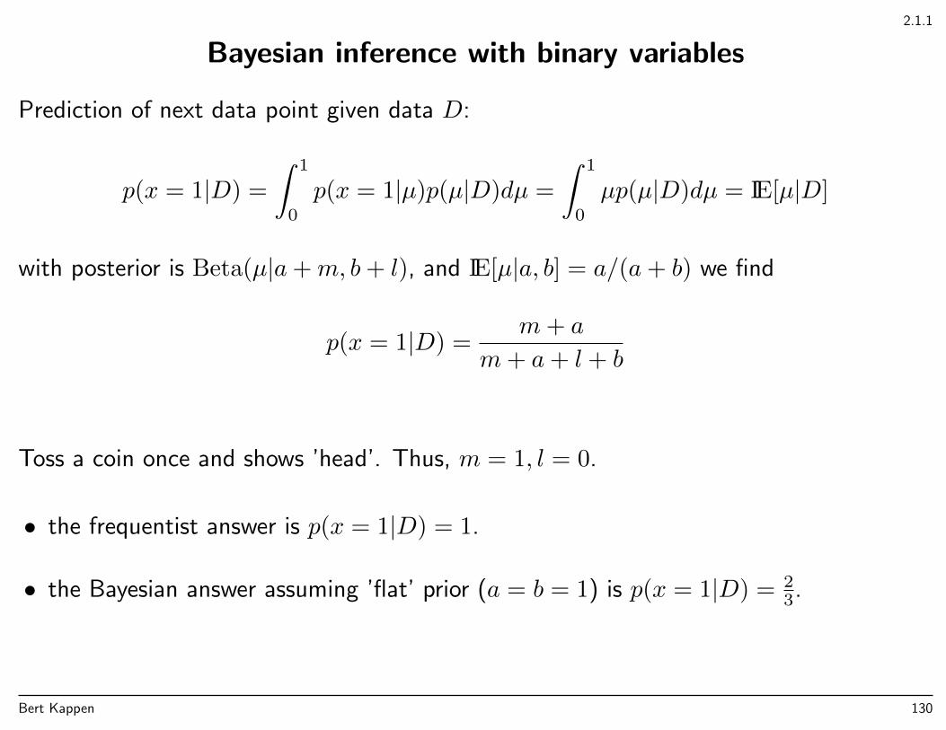
Prediction of next data point given data D:
p(x = 1|D) =
∫ 1
0
p(x = 1|µ)p(µ|D)dµ =
∫ 1
0
µp(µ|D)dµ = IE[µ|D]
with posterior is Beta(µ|a+m, b+ l), and IE[µ|a, b] = a/(a+ b) we find
p(x = 1|D) =m+ a
m+ a+ l + b
Toss a coin once and shows ’head’. Thus, m = 1, l = 0.
• the frequentist answer is p(x = 1|D) = 1.
• the Bayesian answer assuming ’flat’ prior (a = b = 1) is p(x = 1|D) = 23.
Bert Kappen 130

2.2
Multinomial variables
Alternative representation: x ∈ v1, v2, parameter vector: µ = (µ1, µ2), where µ1+µ2 =1.
p(x = vk|µ) = µk
In fancy notation:
p(x|µ) =∏k
µδxvkk
Generalizes to multinomial variables: x ∈ v1, . . . , vK,
µ = (µ1, . . . , µK)∑k
µk = 1
Bert Kappen 131
2.2
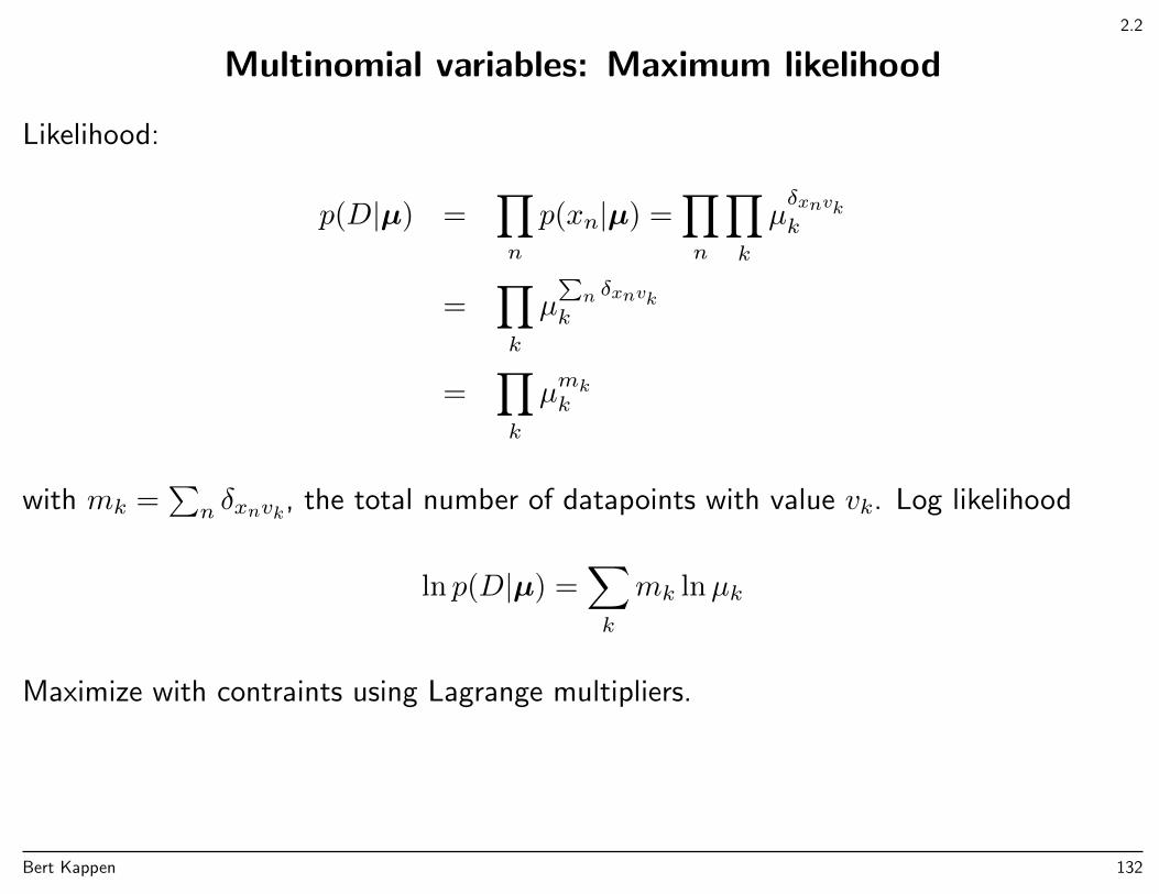
Multinomial variables: Maximum likelihood
Likelihood:
p(D|µ) =∏n
p(xn|µ) =∏n
∏k
µδxnvkk
=∏k
µ∑n δxnvk
k
=∏k
µmkk
with mk =∑n δxnvk, the total number of datapoints with value vk. Log likelihood
ln p(D|µ) =∑k
mk lnµk
Maximize with contraints using Lagrange multipliers.
Bert Kappen 132
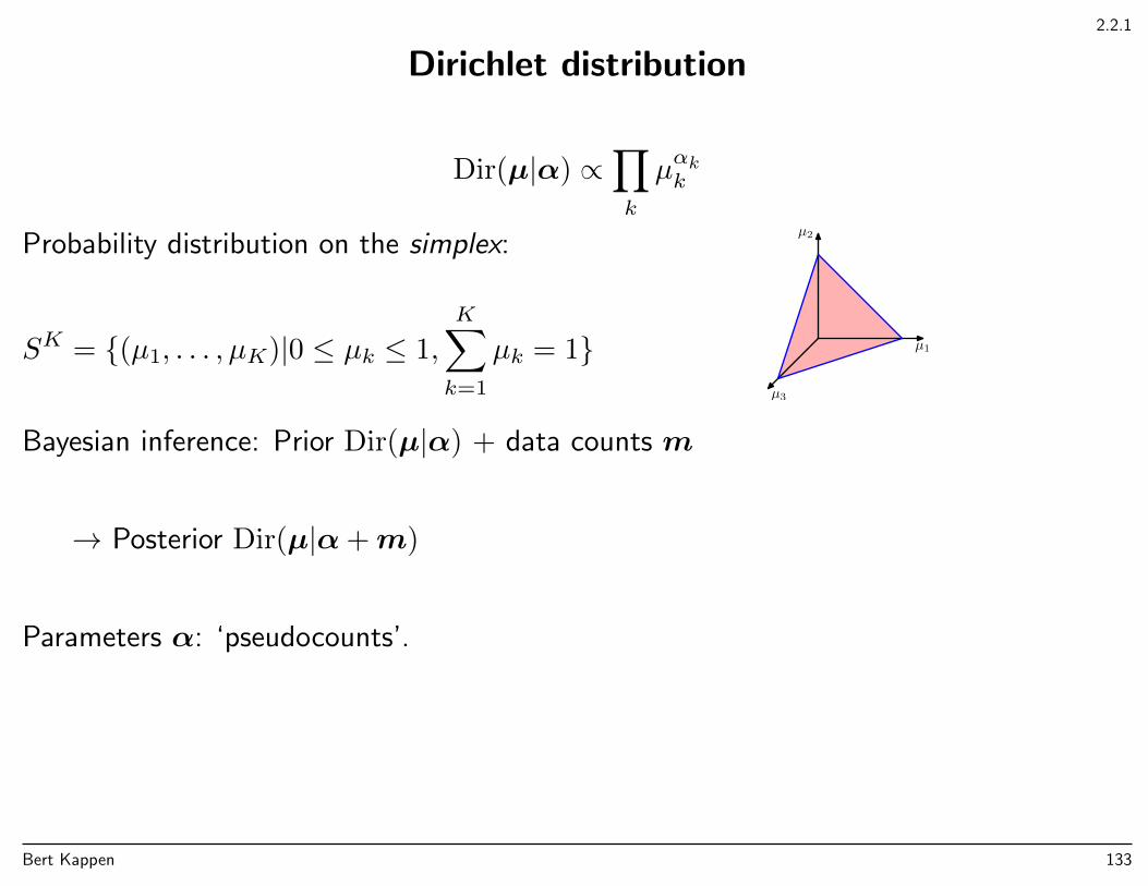
2.2.1
Dirichlet distribution
Dir(µ|α) ∝∏k
µαkk
Probability distribution on the simplex:
SK = (µ1, . . . , µK)|0 ≤ µk ≤ 1,
K∑k=1
µk = 1 µ1
µ2
µ3
Bayesian inference: Prior Dir(µ|α) + data counts m
→ Posterior Dir(µ|α+m)
Parameters α: ‘pseudocounts’.
Bert Kappen 133
2.2.1
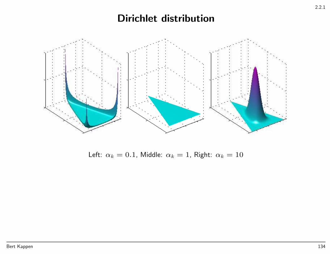
Dirichlet distribution
Left: αk = 0.1, Middle: αk = 1, Right: αk = 10
Bert Kappen 134
2.3
Gaussian
Gaussian distribution
N (x|µ, σ2) =1√
2πσ2exp
− (x− µ)2
2σ2
Specified by µ and σ2
In d dimensions
N (x|µ,Σ) =1
(2π)d/2|Σ|1/2 exp
(−1
2(x− µ)TΣ−1(x− µ)
)
Bert Kappen 135
2.3
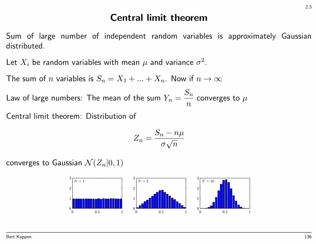
Central limit theorem
Sum of large number of independent random variables is approximately Gaussiandistributed.
Let Xi be random variables with mean µ and variance σ2.
The sum of n variables is Sn = X1 + ...+Xn. Now if n→∞
Law of large numbers: The mean of the sum Yn =Snn
converges to µ
Central limit theorem: Distribution of
Zn =Sn − nµσ√n
converges to Gaussian N (Zn|0, 1)
N = 1
0 0.5 10
1
2
3N = 2
0 0.5 10
1
2
3N = 10
0 0.5 10
1
2
3
Bert Kappen 136
Appendix C
Symmetric matrices
Symmetric matrices:Aij = Aji, AT = A
Inverse of a matrix is a matrix A−1 such that A−1A = AA−1 = I, where I is the identitymatrix.
A−1 is also symmetric:
I = IT = (A−1A)T = AT (A−1)T = A(A−1)T
Thus, (A−1)T = A−1.
Bert Kappen 137
Appendix C
Eigenvalues
A symmetric real-valued d× d matrix has d real eigenvalues λk and d eigenvectors uk:
Auk = λkuk, k = 1, . . . , d
or(A− λkI)uk = 0
Solution of this equation for non-zero uk requires λk to satisfy the characteristic equation:
det(A− λI) = 0
This is a polynomial equation in λ of degree d and has thus d solutions 4 λ1, . . . , λd.
4In general, the solutions are complex. It can be shown that with symmetric matrices, the solutions are in fact real.
Bert Kappen 138
Appendix C
Eigenvectors
Consider two different eigenvectors k and j. Multiply the k-th eigenvalue equation by ujfrom the left:
uTj Auk = λkuTj uk
Multiply the j-th eigenvalue equation by uk from the left:
uTkAuj = λjuTkuj = λju
Tj uk
Subtract(λk − λj)uTj uk = 0
Thus, eigenvectors with different eigenvalues are orthogonal
Bert Kappen 139
Appendix C
If λk = λj then any linear combination is also an eigenvector:
A(αuk + βuj) = λk(αuk + βuj)
This can be used to choose eigenvectors with identical eigenvalues orthogonal.
If uk is an eigenvector of A, then αuk is also an eigenvector of A. Thus, we can makeall eigenvectors the same length one: uTkuk = 1.
In summary,uTj uk = δjk
with δjk the Kronecker delta, is equal to 1 if j=k and zero otherwise.
The eigenvectors span the d-dimensional space as an orthonormal basis.
Bert Kappen 140
Appendix C
Orthogonal matrices
Write U = (u1, . . . ,ud).
U is an orthogonal matrix 5 , i.e.
UTU = I
For orthogonal matrices,
UTUU−1 = U−1 = UT
So UUT = 1, i.e. the transposed is orthogonal as well (note that U is in general notsymmetric).
Furthermore,
det(UUT ) = 1⇒ det(U) det(UT ) = 1
⇒ det(U) = ±1
5
Uij = (uj)i, (UTU)ij =
∑k
(UT
)ikUkj =∑k
UkiUkj =∑k
(ui)k(uj)k = uTi · uj = δij
Bert Kappen 141

Appendix C
Orthogonal matrices implement rigid rotations, i.e. length and angle preserving.
x1 = Ux1 x2 = Ux2
thenxT1 x2 = xT1 U
TUx2 = xT1 x2
Bert Kappen 142
Appendix C
Diagonalization
The eigenvector equation can be written as
AU = A(u1, . . . ,ud) = (Au1, . . . , Aud) = (λ1u1, . . . , λdud)
= (u1, . . . ,ud)
λ1 . . . 0... ...0 . . . λd
= UΛ
By right-multiplying by UT we obtain the important result
A = UΛUT
which can also be written as ’expansion in eigenvectors’
A =
d∑k=1
λkukuTk
Bert Kappen 143

Appendix C
Applications
A = UΛUT ⇒ A2 = UΛUTUΛUT = UΛ2UT
An = UΛnUT A−n = UΛ−nUT
Determinant is product of eigenvalues:
det(A) = det(UΛUT ) = det(U) det(Λ) det(UT ) =∏k
λk
Bert Kappen 144
Appendix C
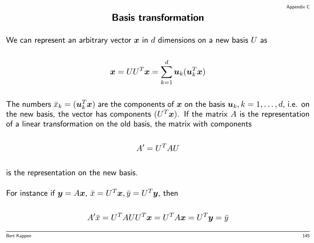
Basis transformation
We can represent an arbitrary vector x in d dimensions on a new basis U as
x = UUTx =
d∑k=1
uk(uTkx)
The numbers xk = (uTkx) are the components of x on the basis uk, k = 1, . . . , d, i.e. onthe new basis, the vector has components (UTx). If the matrix A is the representationof a linear transformation on the old basis, the matrix with components
A′ = UTAU
is the representation on the new basis.
For instance if y = Ax, x = UTx, y = UTy, then
A′x = UTAUUTx = UTAx = UTy = y
Bert Kappen 145
Appendix C
So a matrix is diagonal on a basis of its eigenvectors:
A′ = UTAU = UTUΛUTU = Λ
Bert Kappen 146
2.3
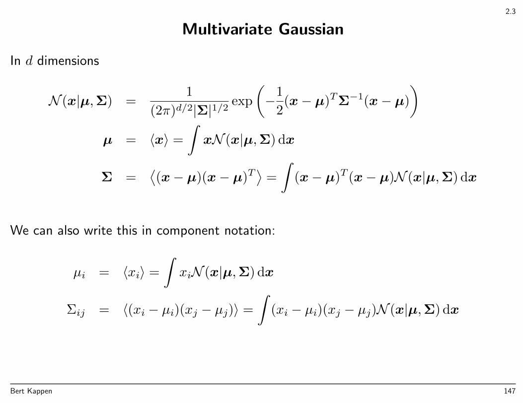
Multivariate Gaussian
In d dimensions
N (x|µ,Σ) =1
(2π)d/2|Σ|1/2 exp
(−1
2(x− µ)TΣ−1(x− µ)
)µ = 〈x〉 =
∫xN (x|µ,Σ) dx
Σ =⟨(x− µ)(x− µ)T
⟩=
∫(x− µ)T (x− µ)N (x|µ,Σ) dx
We can also write this in component notation:
µi = 〈xi〉 =
∫xiN (x|µ,Σ) dx
Σij = 〈(xi − µi)(xj − µj)〉 =
∫(xi − µi)(xj − µj)N (x|µ,Σ) dx
Bert Kappen 147
2.3, p. 80
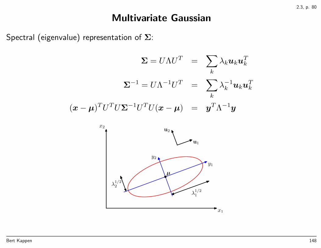
Multivariate Gaussian
Spectral (eigenvalue) representation of Σ:
Σ = UΛUT =∑k
λkukuTk
Σ−1 = UΛ−1UT =∑k
λ−1k uku
Tk
(x− µ)TUTUΣ−1UTU(x− µ) = yTΛ−1y
x1
x2
λ1/21
λ1/22
y1
y2
u1
u2
µ
Bert Kappen 148
2.3, p. 81
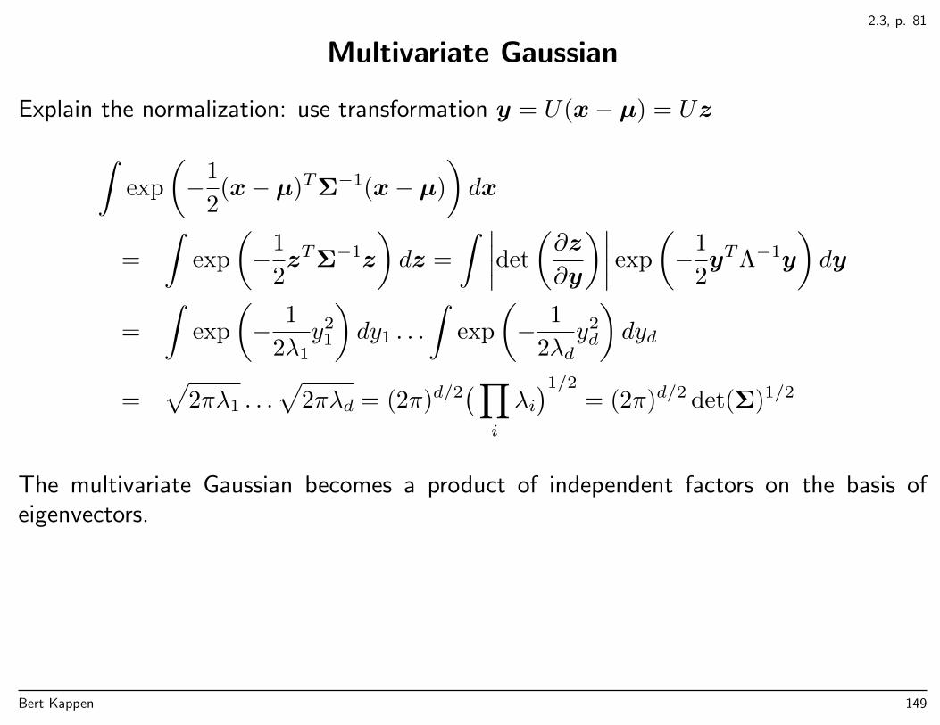
Multivariate Gaussian
Explain the normalization: use transformation y = U(x− µ) = Uz∫exp
(−1
2(x− µ)TΣ−1(x− µ)
)dx
=
∫exp
(−1
2zTΣ−1z
)dz =
∫ ∣∣∣∣det
(∂z
∂y
)∣∣∣∣ exp
(−1
2yTΛ−1y
)dy
=
∫exp
(− 1
2λ1y2
1
)dy1 . . .
∫exp
(− 1
2λdy2d
)dyd
=√
2πλ1 . . .√
2πλd = (2π)d/2(∏
i
λi)1/2
= (2π)d/2 det(Σ)1/2
The multivariate Gaussian becomes a product of independent factors on the basis ofeigenvectors.
Bert Kappen 149
2.3, p. 82
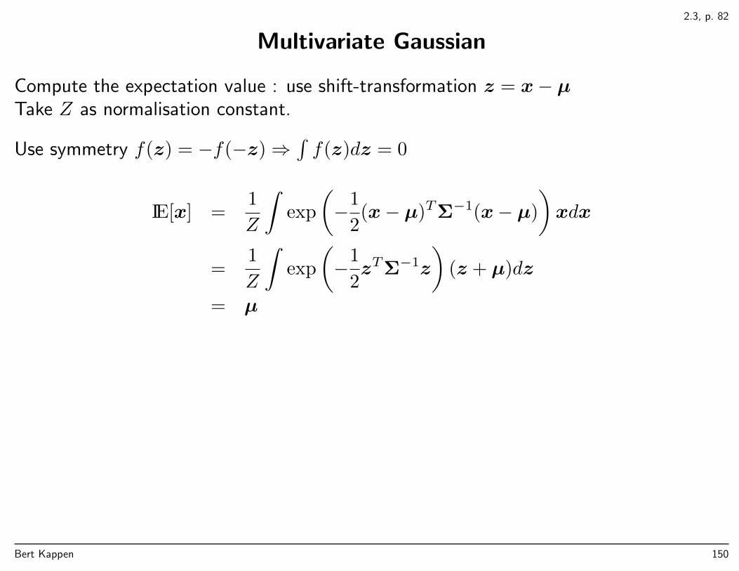
Multivariate Gaussian
Compute the expectation value : use shift-transformation z = x− µTake Z as normalisation constant.
Use symmetry f(z) = −f(−z)⇒∫f(z)dz = 0
IE[x] =1
Z
∫exp
(−1
2(x− µ)TΣ−1(x− µ)
)xdx
=1
Z
∫exp
(−1
2zTΣ−1z
)(z + µ)dz
= µ
Bert Kappen 150
2.3, p. 82
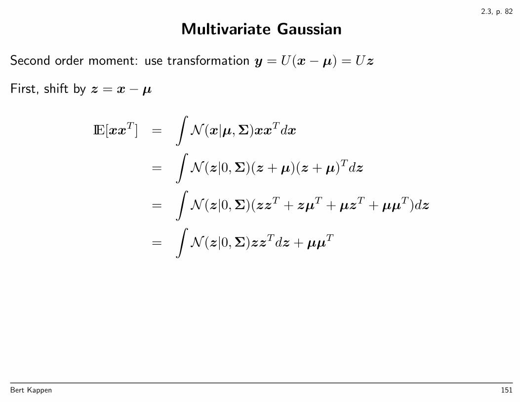
Multivariate Gaussian
Second order moment: use transformation y = U(x− µ) = Uz
First, shift by z = x− µ
IE[xxT ] =
∫N (x|µ,Σ)xxTdx
=
∫N (z|0,Σ)(z + µ)(z + µ)Tdz
=
∫N (z|0,Σ)(zzT + zµT + µzT + µµT )dz
=
∫N (z|0,Σ)zzTdz + µµT
Bert Kappen 151
2.3, p. 82
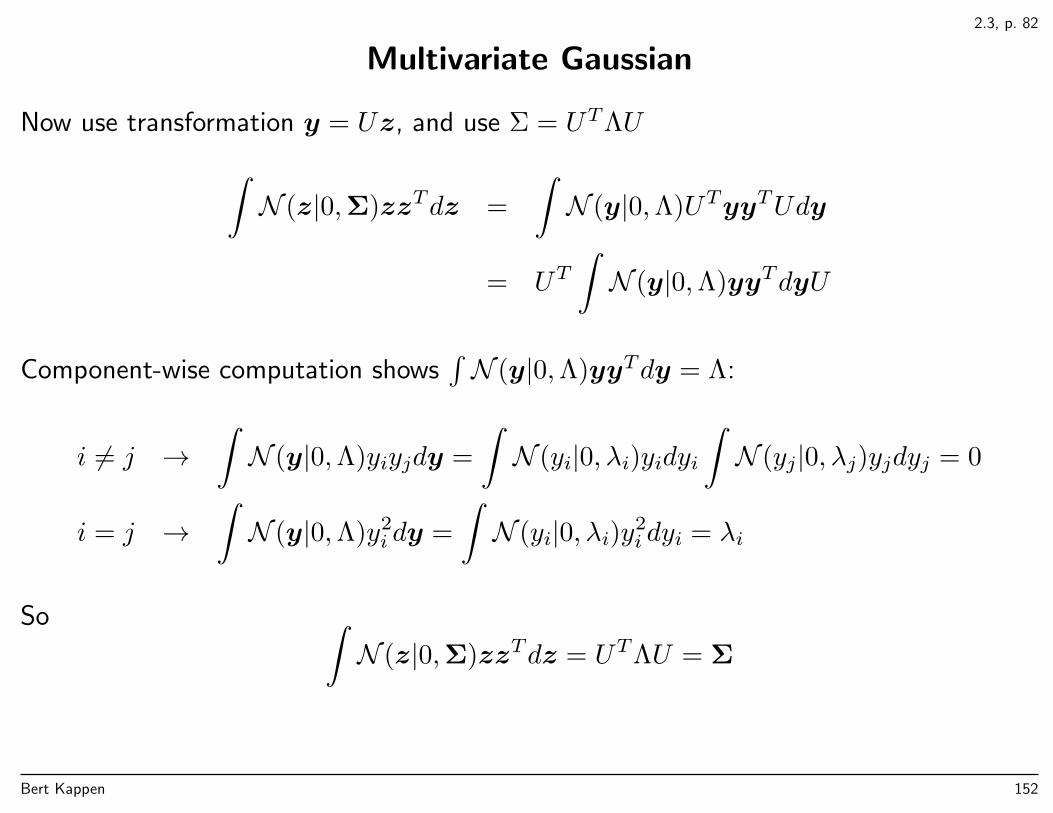
Multivariate Gaussian
Now use transformation y = Uz, and use Σ = UTΛU∫N (z|0,Σ)zzTdz =
∫N (y|0,Λ)UTyyTUdy
= UT∫N (y|0,Λ)yyTdyU
Component-wise computation shows∫N (y|0,Λ)yyTdy = Λ:
i 6= j →∫N (y|0,Λ)yiyjdy =
∫N (yi|0, λi)yidyi
∫N (yj|0, λj)yjdyj = 0
i = j →∫N (y|0,Λ)y2
i dy =
∫N (yi|0, λi)y2
i dyi = λi
So ∫N (z|0,Σ)zzTdz = UTΛU = Σ
Bert Kappen 152
2.3, p. 82
Multivariate Gaussian
So, second moment isIE[xxT ] = Σ + µµT
Covariancecov[x] = IE[xxT ]− IE[x]IE[x]T = Σ
Bert Kappen 153
2.3, p. 84
Multivariate Gaussian
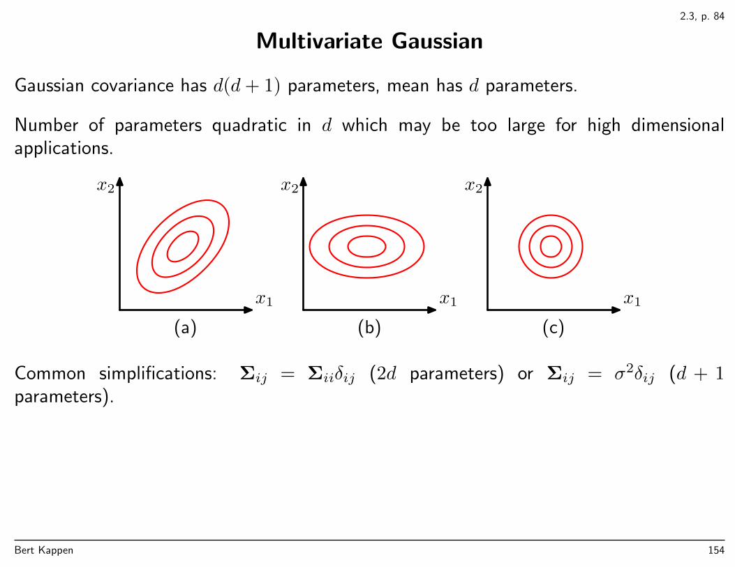
Gaussian covariance has d(d+ 1) parameters, mean has d parameters.
Number of parameters quadratic in d which may be too large for high dimensionalapplications.
x1
x2
(a)
x1
x2
(b)
x1
x2
(c)
Common simplifications: Σij = Σiiδij (2d parameters) or Σij = σ2δij (d + 1parameters).
Bert Kappen 154

2.3.1
Conditional of Gaussian is Gaussian
Exponent in Gaussian N (x|µ,Σ): quadratic form
−1
2(x− µ)TΣ−1(x− µ) = −1
2xTΣ−1x+ xTΣ−1µ+ c = −1
2xTKx+ xTKµ+ c
Precision matrix K = Σ−1, nb: Conditional
p(xa|xb) =p(xa,xb)
p(xb)∝ p(xa,xb)
Exponent of conditional: collect all terms with xa, ignore constants, regard xb asconstant, and write in quadratic form as above
−1
2xTaKa|bxa + xTaKa|bµa|b = −1
2xTaKaaxa + xTaKaaµa − xTaKab(xb − µb)
= −1
2xTaKaaxa + xTaKaa(µa −K−1
aaKab(xb − µb))
Bert Kappen 155
2.3.2
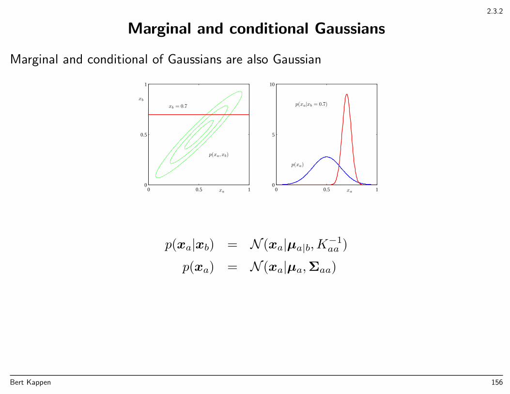
Marginal and conditional Gaussians
Marginal and conditional of Gaussians are also Gaussian
xa
xb = 0.7
xb
p(xa, xb)
0 0.5 10
0.5
1
xa
p(xa)
p(xa|xb = 0.7)
0 0.5 10
5
10
p(xa|xb) = N (xa|µa|b,K−1aa )
p(xa) = N (xa|µa,Σaa)
Bert Kappen 156
2.3.1
Some matrix identities
(A BC D
)−1
=
(M −MBD−1
−D−1CM D−1 +D−1CMBD−1
)
with M =(A−BD−1C
)−1.
(Kaa Kab
Kba Kbb
)=
(Σaa ΣabΣba Σbb
)−1
=
(M −MΣabΣ
−1bb
−Σ−1bb ΣbaM Σ−1
bb + Σ−1bb ΣbaMΣabΣ
−1bb
)
with M =(Σaa − ΣabΣ
−1bb Σba
)−1.
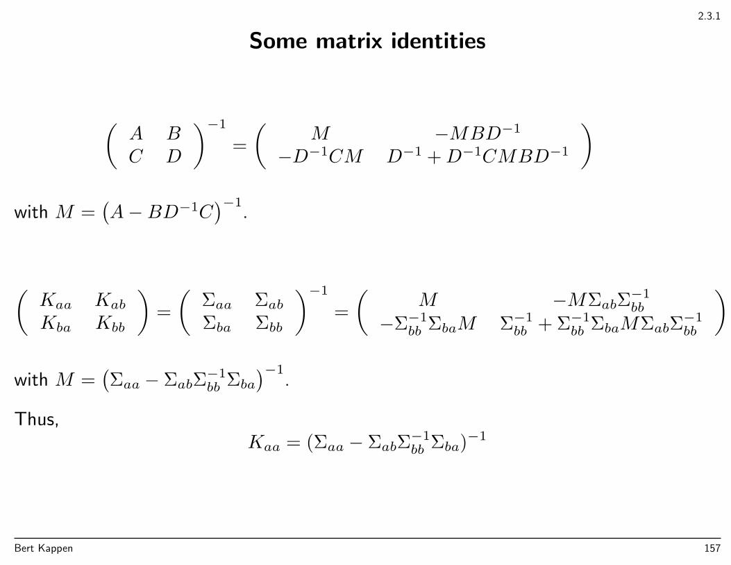
Thus,Kaa = (Σaa − ΣabΣ
−1bb Σba)
−1
Bert Kappen 157
2.3.3, p. 93
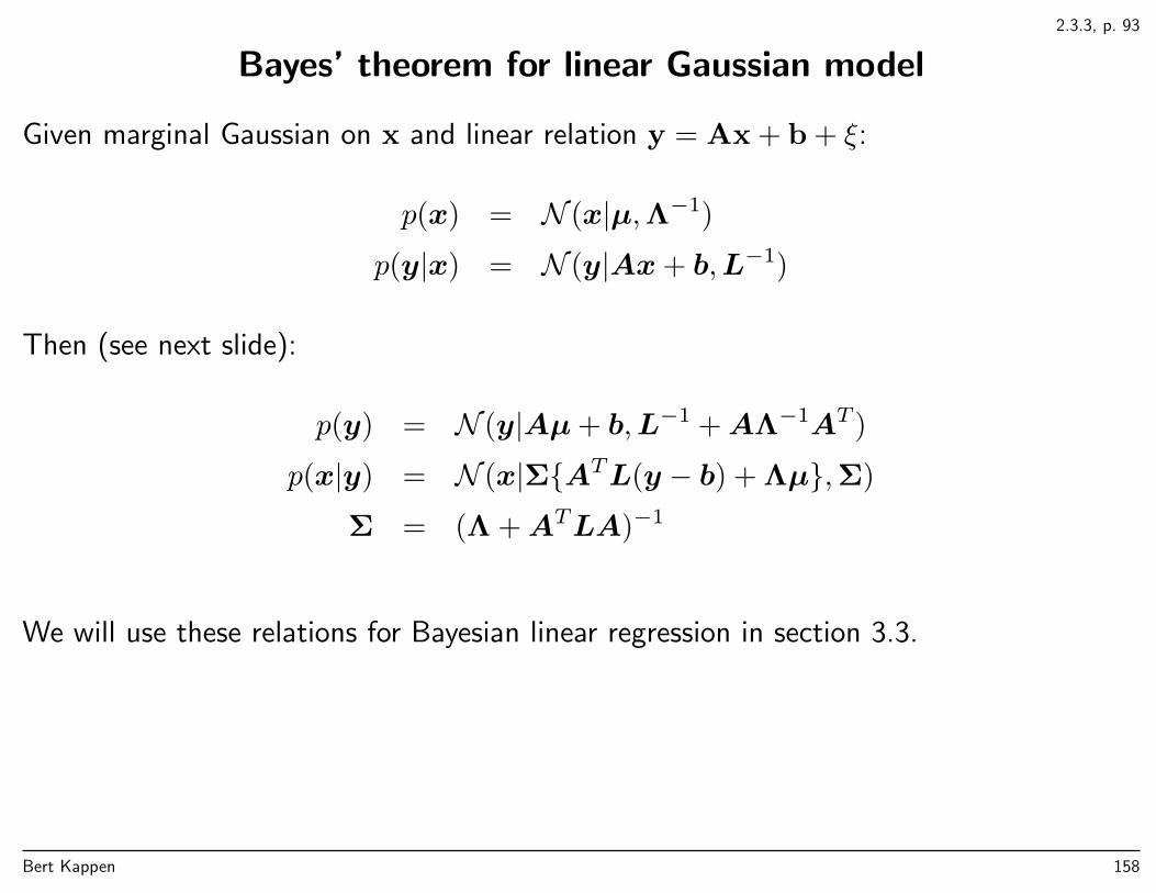
Bayes’ theorem for linear Gaussian model
Given marginal Gaussian on x and linear relation y = Ax + b + ξ:
p(x) = N (x|µ,Λ−1)
p(y|x) = N (y|Ax+ b,L−1)
Then (see next slide):
p(y) = N (y|Aµ+ b,L−1 +AΛ−1AT )
p(x|y) = N (x|ΣATL(y − b) + Λµ,Σ)
Σ = (Λ +ATLA)−1
We will use these relations for Bayesian linear regression in section 3.3.
Bert Kappen 158
2.3.3, p. 93
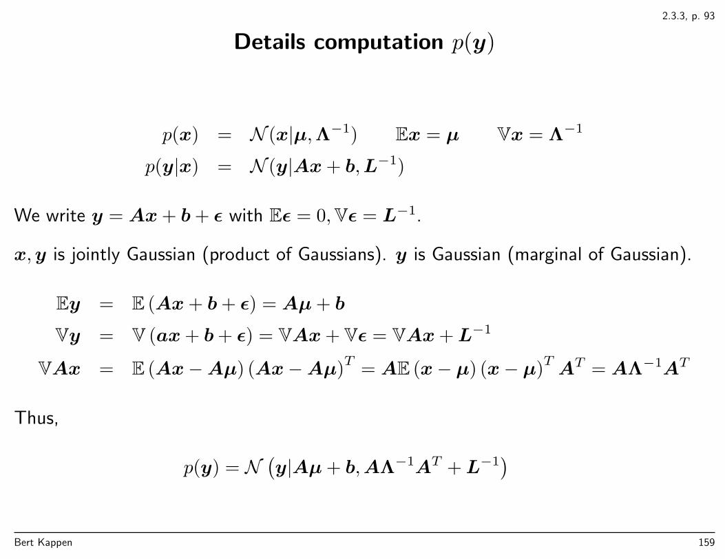
Details computation p(y)
p(x) = N (x|µ,Λ−1) Ex = µ Vx = Λ−1
p(y|x) = N (y|Ax+ b,L−1)
We write y = Ax+ b+ ε with Eε = 0,Vε = L−1.
x,y is jointly Gaussian (product of Gaussians). y is Gaussian (marginal of Gaussian).
Ey = E (Ax+ b+ ε) = Aµ+ b
Vy = V (ax+ b+ ε) = VAx+ Vε = VAx+L−1
VAx = E (Ax−Aµ) (Ax−Aµ)T
= AE (x− µ) (x− µ)TAT = AΛ−1AT
Thus,
p(y) = N(y|Aµ+ b,AΛ−1AT +L−1
)Bert Kappen 159
2.3.3, p. 93
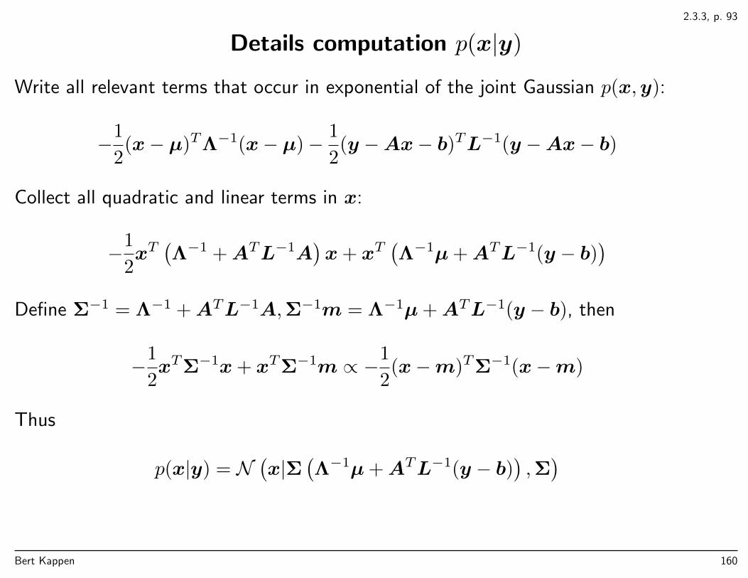
Details computation p(x|y)
Write all relevant terms that occur in exponential of the joint Gaussian p(x,y):
−1
2(x− µ)TΛ−1(x− µ)− 1
2(y −Ax− b)TL−1(y −Ax− b)
Collect all quadratic and linear terms in x:
−1
2xT(Λ−1 +ATL−1A
)x+ xT
(Λ−1µ+ATL−1(y − b)
)Define Σ−1 = Λ−1 +ATL−1A,Σ−1m = Λ−1µ+ATL−1(y − b), then
−1
2xTΣ−1x+ xTΣ−1m ∝ −1
2(x−m)TΣ−1(x−m)
Thus
p(x|y) = N(x|Σ
(Λ−1µ+ATL−1(y − b)
),Σ)
Bert Kappen 160
2.3.6
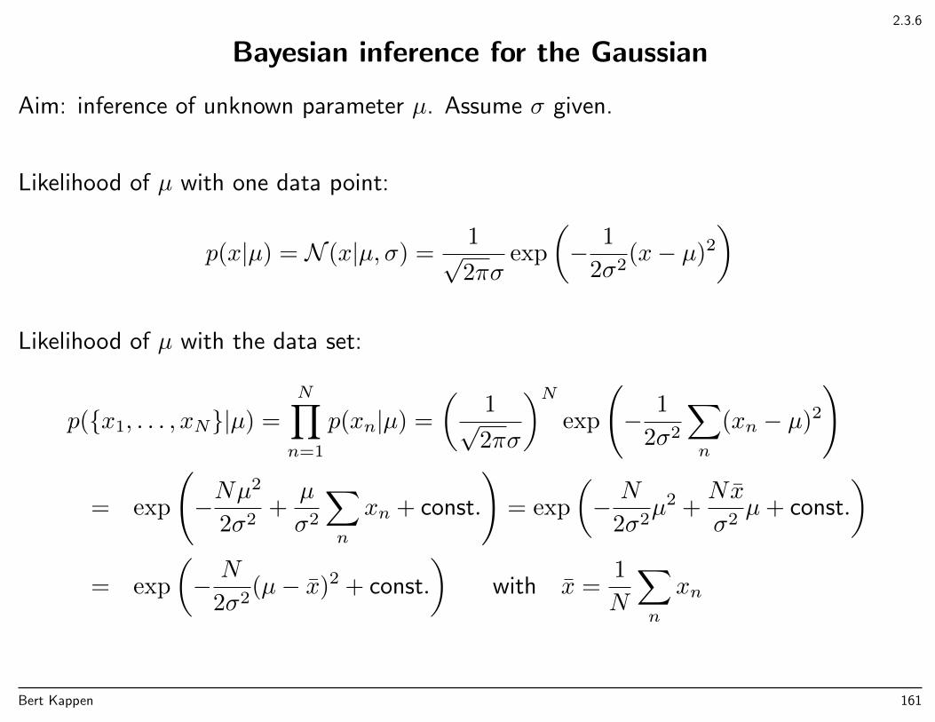
Bayesian inference for the Gaussian
Aim: inference of unknown parameter µ. Assume σ given.
Likelihood of µ with one data point:
p(x|µ) = N (x|µ, σ) =1√2πσ
exp
(− 1
2σ2(x− µ)2
)
Likelihood of µ with the data set:
p(x1, . . . , xN|µ) =
N∏n=1
p(xn|µ) =
(1√2πσ
)Nexp
(− 1
2σ2
∑n
(xn − µ)2
)
= exp
(−Nµ
2
2σ2+µ
σ2
∑n
xn + const.
)= exp
(− N
2σ2µ2 +
Nx
σ2µ+ const.
)= exp
(− N
2σ2(µ− x)2 + const.
)with x =
1
N
∑n
xn
Bert Kappen 161
2.3.6
Bayesian inference for the Gaussian
Likelihood:
p(Data|µ) = exp
(− N
2σ2(µ− x)2 + const.
)Prior:
p(µ) = N (µ|µ0, σ0) =1√
2πσ0
exp
(− 1
2σ20
(µ− µ0)2
)
µ0, σ0 hyperparameters. Large σ0 = large prior uncertainty in µ.
p(µ|Data) ∝ p(Data|µ)p(µ)
Bert Kappen 162
2.3.6, pp. 97-98
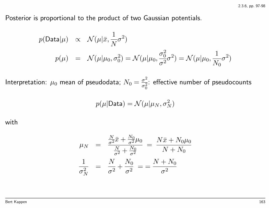
Posterior is proportional to the product of two Gaussian potentials.
p(Data|µ) ∝ N (µ|x, 1
Nσ2)
p(µ) = N (µ|µ0, σ20) = N (µ|µ0,
σ20
σ2σ2) = N (µ|µ0,
1
N0σ2)
Interpretation: µ0 mean of pseudodata; N0 = σ2
σ20: effective number of pseudocounts
p(µ|Data) = N (µ|µN , σ2N)
with
µN =Nσ2x+ N0
σ2µ0
Nσ2 + N0
σ2
=Nx+N0µ0
N +N0
1
σ2N
=N
σ2+N0
σ2= =
N +N0
σ2
Bert Kappen 163
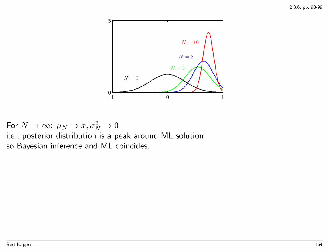
2.3.6, pp. 98-99
N = 0
N = 1
N = 2
N = 10
−1 0 10
5
For N →∞: µN → x, σ2N → 0
i.e., posterior distribution is a peak around ML solutionso Bayesian inference and ML coincides.
Bert Kappen 164
2.3.6, pp. 100-102
Posterior in µ, σ2
p(Data|µ, λ) =
N∏n=1
(λ
2π
)1/2
exp
(−λ
2(xn − µ)2
)
∝(λ1/2 exp
(−λµ
2
2
))Nexp
(λµ
N∑n=1
xn −λ
2
N∑n=1
x2n
)
Conjugate prior
p(µ, λ) ∝(λ1/2 exp
(−λµ
2
2
))βexp(cλµ− dλ)
∝ λ1/2 exp
(−λβ
2(µ− c/β)2
)λβ−1
2 exp
(−(d− c2
2β)λ
)∝ N (µ|c/β, (λβ)−1)Gam(λ|a, b)
with a− 1 = (β − 1)/2, b = d− c2
2β . 6
6Gam(λ|a, b) ∝ λa−1 exp(−bλ)
Bert Kappen 165
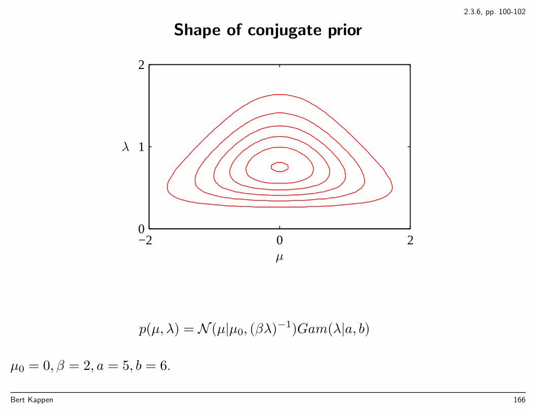
2.3.6, pp. 100-102
Shape of conjugate prior
µ
λ
−2 0 20
1
2
p(µ, λ) = N (µ|µ0, (βλ)−1)Gam(λ|a, b)
µ0 = 0, β = 2, a = 5, b = 6.
Bert Kappen 166
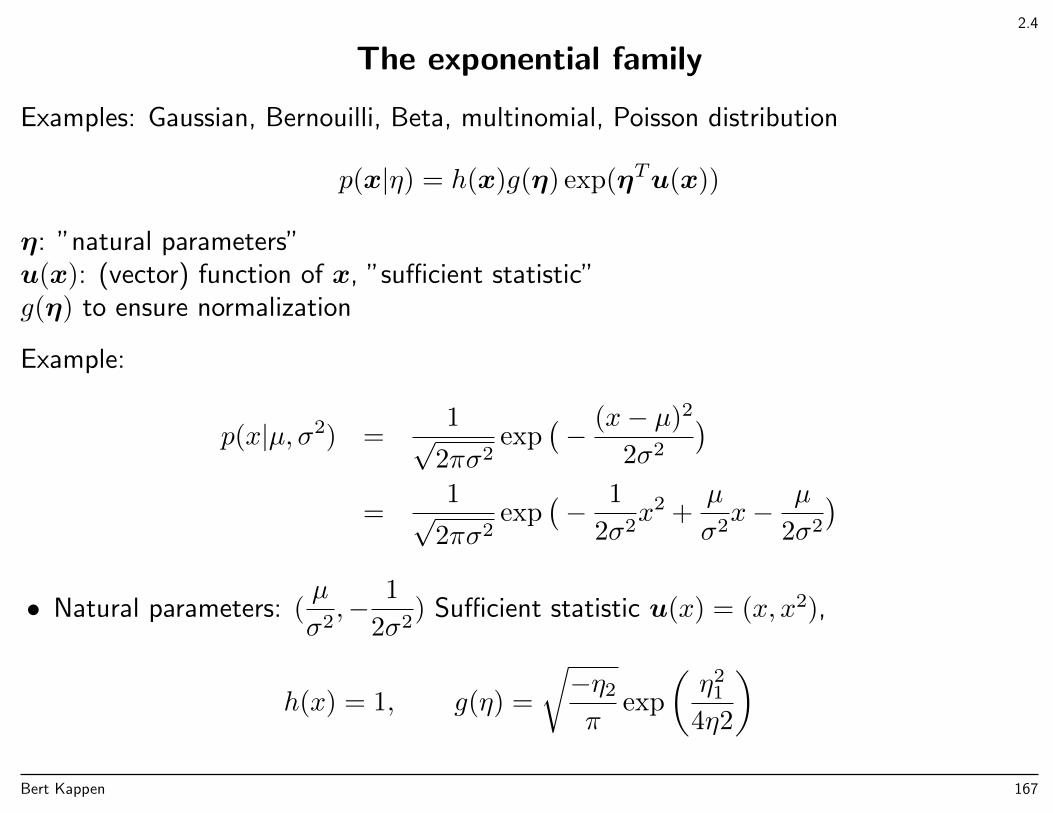
2.4
The exponential family
Examples: Gaussian, Bernouilli, Beta, multinomial, Poisson distribution
p(x|η) = h(x)g(η) exp(ηTu(x))
η: ”natural parameters”u(x): (vector) function of x, ”sufficient statistic”g(η) to ensure normalization
Example:
p(x|µ, σ2) =1√
2πσ2exp
(− (x− µ)2
2σ2
)=
1√2πσ2
exp(− 1
2σ2x2 +
µ
σ2x− µ
2σ2
)• Natural parameters: (
µ
σ2,− 1
2σ2) Sufficient statistic u(x) = (x, x2),
h(x) = 1, g(η) =
√−η2
πexp
(η2
1
4η2
)Bert Kappen 167
2.4.1
The exponential family / Maximum likelihood and sufficientstatistics
In the ML solution η = ηML, the likelihood is stationary:
∇η∑n
log p(xn|η) = 0
Since
∇η log p(xn|η) = ∇η log(h(xn)g(η) exp(ηTu(xn))
)= ∇η log g(η) + u(xn)
this implies that in ML solution η = ηML
−∇η log g(η) =1
N
∑n
u(xn)
Bert Kappen 168
2.4.1
Now, g(η) is the normalization factor, i.e.,
g(η)−1 =
∫h(x) exp(ηTu(x))dx
So
−∇η log g(η) = ∇η log g(η)−1 = g(η)∇η∫h(x) exp(ηTu(x))
= g(η)
∫h(x)u(x) exp(ηTu(x))
=
∫u(x)p(x|η)dx = 〈u(x)〉η
and we have that in the ML solution:
1
N
∑n
u(xn) = 〈u(x)〉ηML”Moment matching”
ML estimator depends on data only through sufficient statistics∑nu(xn)
Bert Kappen 169
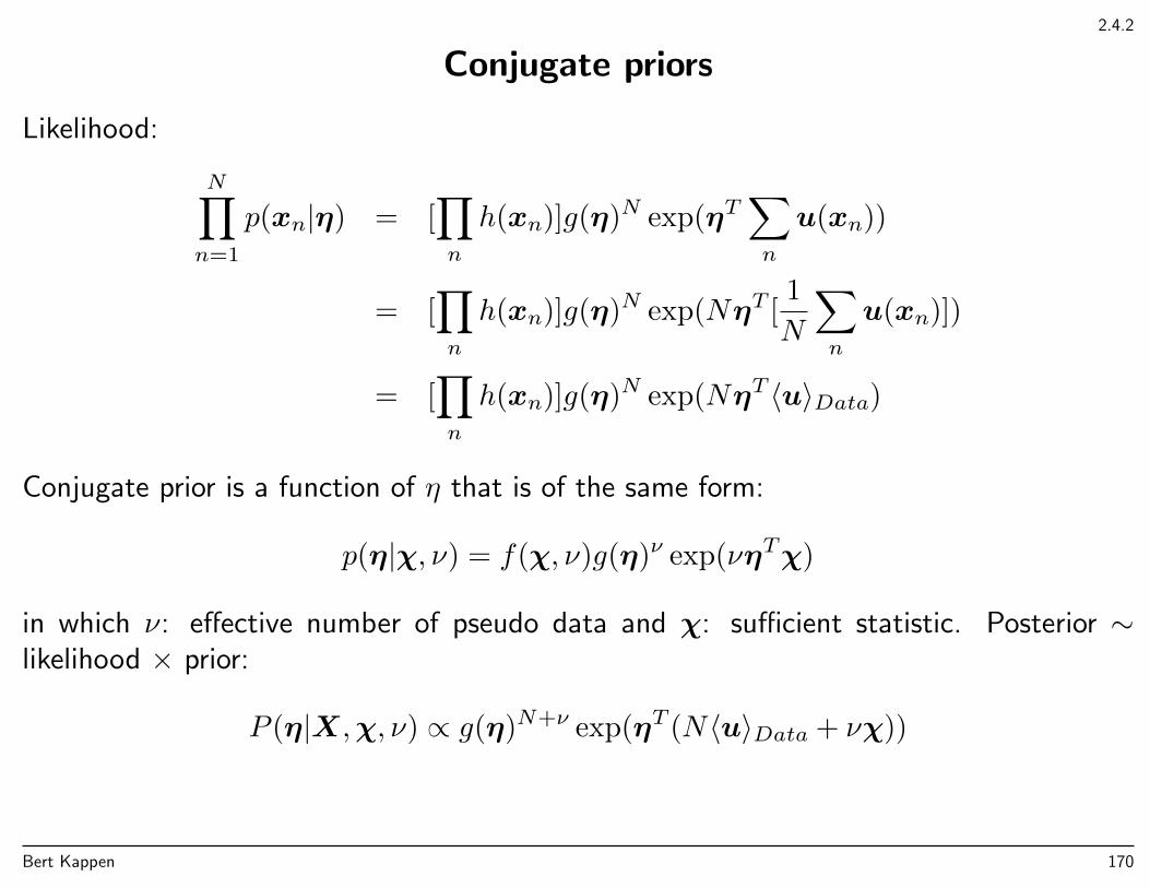
2.4.2
Conjugate priors
Likelihood:
N∏n=1
p(xn|η) = [∏n
h(xn)]g(η)N exp(ηT∑n
u(xn))
= [∏n
h(xn)]g(η)N exp(NηT [1
N
∑n
u(xn)])
= [∏n
h(xn)]g(η)N exp(NηT 〈u〉Data)
Conjugate prior is a function of η that is of the same form:
p(η|χ, ν) = f(χ, ν)g(η)ν exp(νηTχ)
in which ν: effective number of pseudo data and χ: sufficient statistic. Posterior ∼likelihood × prior:
P (η|X,χ, ν) ∝ g(η)N+ν exp(ηT (N〈u〉Data + νχ))
Bert Kappen 170
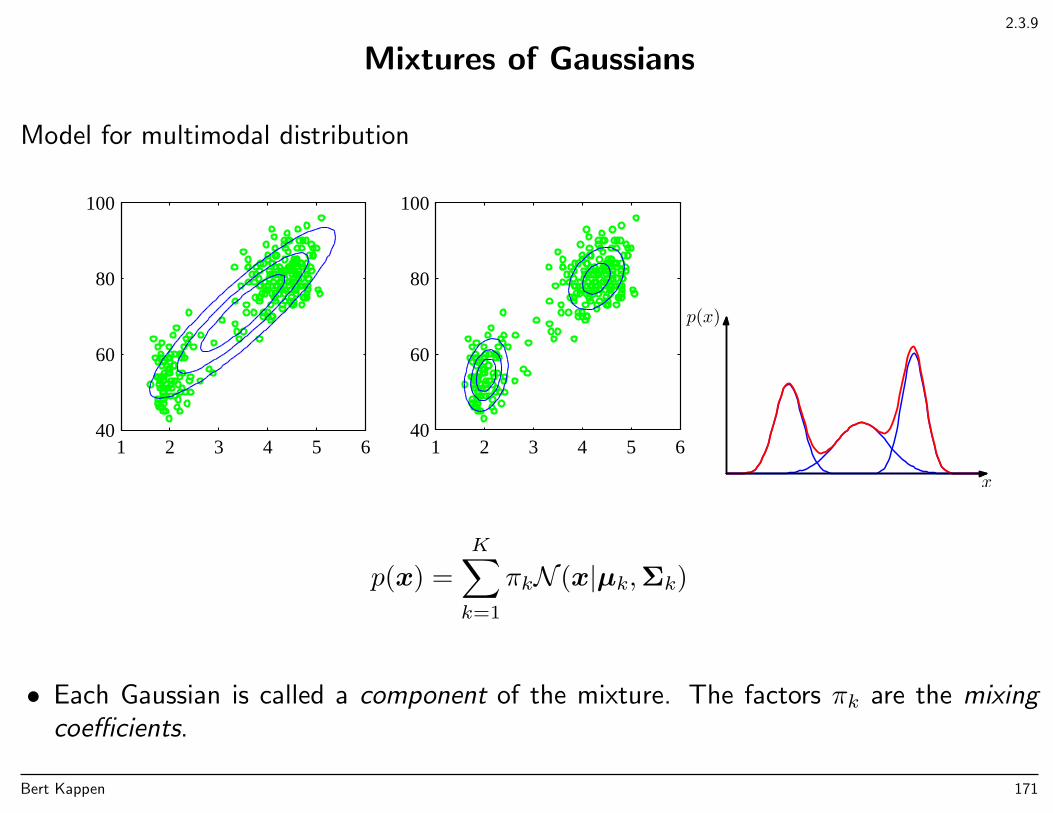
2.3.9
Mixtures of Gaussians
Model for multimodal distribution
1 2 3 4 5 640
60
80
100
1 2 3 4 5 640
60
80
100
x
p(x)
p(x) =
K∑k=1
πkN (x|µk,Σk)
• Each Gaussian is called a component of the mixture. The factors πk are the mixingcoefficients.
Bert Kappen 171
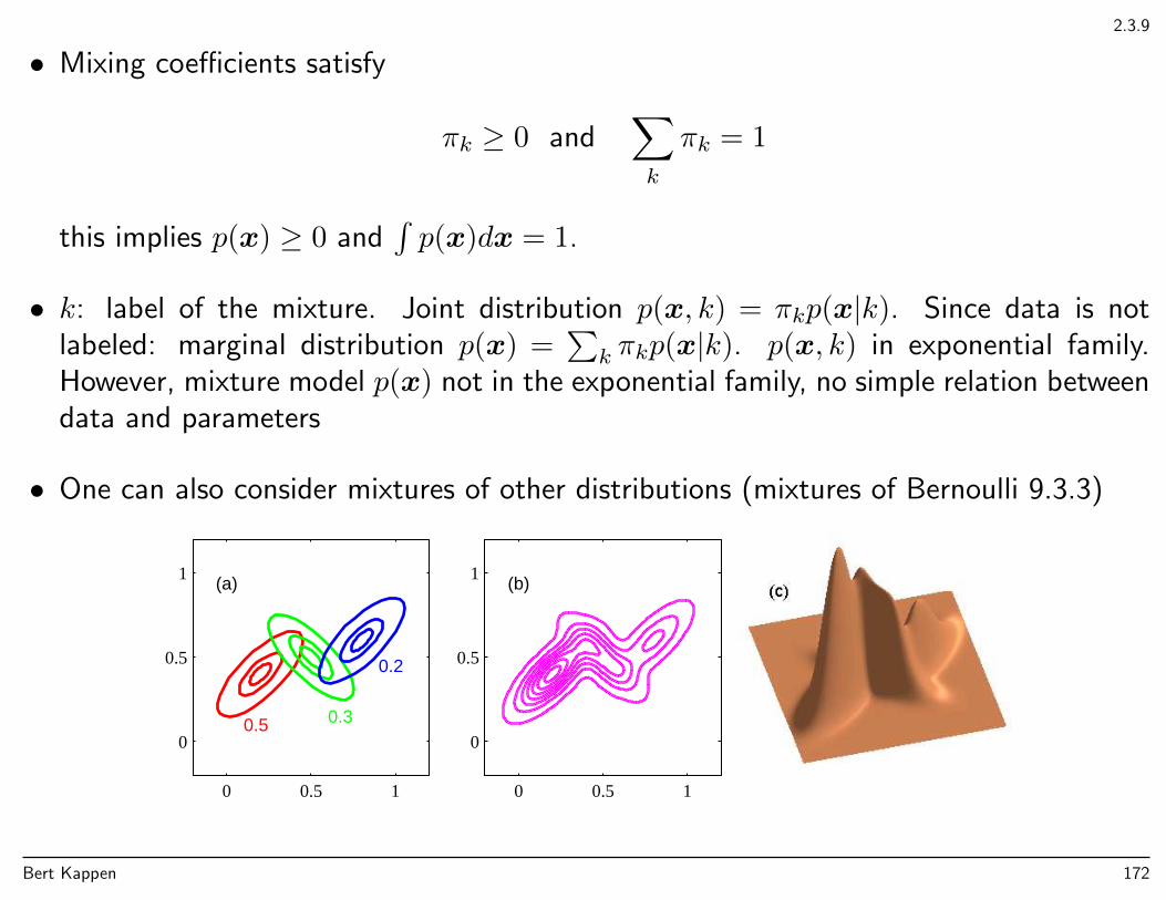
2.3.9
• Mixing coefficients satisfy
πk ≥ 0 and∑k
πk = 1
this implies p(x) ≥ 0 and∫p(x)dx = 1.
• k: label of the mixture. Joint distribution p(x, k) = πkp(x|k). Since data is notlabeled: marginal distribution p(x) =
∑k πkp(x|k). p(x, k) in exponential family.
However, mixture model p(x) not in the exponential family, no simple relation betweendata and parameters
• One can also consider mixtures of other distributions (mixtures of Bernoulli 9.3.3)
0.5 0.3
0.2
(a)
0 0.5 1
0
0.5
1 (b)
0 0.5 1
0
0.5
1
Bert Kappen 172
2.3.9
Mixtures of Gaussians
ML: by gradient ascent (numerical function maximization).
Learning with hidden variables is generally difficult (slow).
Instead, EM (Expectation Maximization) algorithm to deal with hidden variables.
For instance using Bayes’ rule compute the ”soft assignment’ of data xn to each of theclusters:
γk(xn) ≡ p(k|xn) =πkN (xn|µk,Σk)∑k′ πk′N (xn|µk′,Σk′)
update according to
µk =
∑Nn=1 γk(xn)xn∑Nn=1 γk(xn)
See Chapter 9 for more details.
Bert Kappen 173
3
Chapter 3
Linear Models for RegressionRegression: . . . ?
Bert Kappen 174
3
Chapter 3
Linear Models for RegressionRegression: predicting the value of continuous target/output variables given values of theinput variables.
In other words: given a training set of input/output pairs, constructing a function thatmaps input values to continuous output values.
Bert Kappen 175
3.1
Linear Basis Function Models
Linear regression:
y(x,w) = w0 + w1x1 + w2x2 + · · ·+ wDxD = w0 +
D∑j=1
wjxj
Linear in parameters w, and “almost” linear (affine) in input x.
Q: how can we generalize this to models that need not be linear in input x?
Bert Kappen 176
3.1
Linear Basis Function Models
Linear regression:
y(x,w) = w0 + w1x1 + w2x2 + · · ·+ wDxD = w0 +
D∑j=1
wjxj
Linear in parameters w, and “almost” linear (affine) in input x.
Q: how can we generalize this to models that need not be linear in input x? A:
y(x,w) = w0 +
M−1∑j=1
wjφj(x)
where φ1(x), . . . , φM−1(x) are basis functions or feature functions. Defining φ0(x) = 1,we can write it more compactly:
y(x,w) =
M−1∑j=0
wjφj(x) = wTφ(x)
Note: still linear in parameters w! Examples of basis functions?
Bert Kappen 177
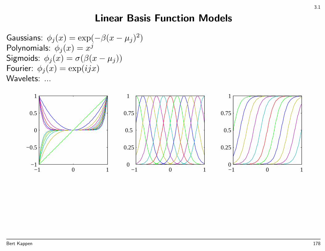
3.1
Linear Basis Function Models
Gaussians: φj(x) = exp(−β(x− µj)2)Polynomials: φj(x) = xj
Sigmoids: φj(x) = σ(β(x− µj))Fourier: φj(x) = exp(ijx)Wavelets: ...
−1 0 1−1
−0.5
0
0.5
1
−1 0 10
0.25
0.5
0.75
1
−1 0 10
0.25
0.5
0.75
1
Bert Kappen 178
3.1.1
Adding some noise
Let’s make some noise. . . and assume the following model:
t = y(x,w) + ε, y(x,w) = wTφ(x)
where we added Gaussian noise ε ∼ N (0, β−1).
Q: what is the distribution of t, given x,w, β?
Bert Kappen 179
3.1.1
Adding some noise
Let’s make some noise. . . and assume the following model:
t = y(x,w) + ε, y(x,w) = wTφ(x)
where we added Gaussian noise ε ∼ N (0, β−1).
Q: what is the distribution of t, given x,w, β?
p(t|x,w, β) = N (t|y(x,w), β−1)
Q: what is the conditional mean IE(t|x)?
Bert Kappen 180
3.1.1
Adding some noise
Let’s make some noise. . . and assume the following model:
t = y(x,w) + ε, y(x,w) = wTφ(x)
where we added Gaussian noise ε ∼ N (0, β−1).
Q: what is the distribution of t, given x,w, β?
p(t|x,w, β) = N (t|y(x,w), β−1)
Q: what is the conditional mean IE(t|x,w, β)?
IE(t|x,w, β) =
∫tp(t|x) dt = y(x,w)
Bert Kappen 181
3.1.1
Maximum likelihood: least squares
Q: What is the likelihood of a data set (xn, tn)Nn=1?
Bert Kappen 182
3.1.1
Maximum likelihood: least squares
Q: What is the likelihood of a data set (xn, tn)Nn=1?
p(t|X,w, β) =
N∏n=1
N(tn|wTφ(xn), β−1
)
Q: How does the log-likelihood depend on the parameters w?
Bert Kappen 183
3.1.1
Maximum likelihood: least squares
Q: What is the likelihood of a data set (xi, ti)Nn=1?
p(t|X,w, β) =
N∏n=1
N(tn|wTφ(xn), β−1
)
Q: How does the log-likelihood depend on the parameters w?
ln p(t|X,w, β) = C − 1
2β
N∑n=1
(tn −wTφ(xn)
)2︸ ︷︷ ︸
sum-of-squares error function
Q: How to optimize the log-likelihood with respect to parameters w?
Bert Kappen 184
3.1.1
Maximum likelihood: least squares
Q: What is the likelihood of a data set (xi, ti)Ni=1?
p(t|X,w, β) =
N∏n=1
N(tn|wTφ(xn), β−1
)Q: How does the log-likelihood depend on the parameters w?
ln p(t|X,w, β) = C − 1
2β
N∑n=1
(tn −wTφ(xn)
)2︸ ︷︷ ︸
sum-of-squares error function
Q: How to optimize the log-likelihood with respect to parameters w?A: differentiate with respect to w and set to zero:
∇w ln p(t|X,w, β) = −βN∑n=1
(tn −wTφ(xn)
)φ(xn)T = 0
Bert Kappen 185
3.1.1
Maximum likelihood: least squares
Rewriting:
0 =
N∑n=1
tnφ(xn)T −wT
(N∑n=1
φ(xn)φ(xn)T
)Solving for w:
wML = (ΦTΦ)−1ΦT︸ ︷︷ ︸Moore-Penrose pseudo-inverse
t
where Φ is an N ×M matrix, the design matrix, with elements Φnj = φj(xn):
Φ =
φ0(x1) φ1(x1) . . . φM−1(x1)φ0(x2) φ1(x2) . . . φM−1(x2)
... ... . . . ...φ0(xN) φ1(xN) . . . φM−1(xN)
Also, one can derive:
β−1ML =
1
N
N∑n=1
(tn −wT
MLφ(xn))2.
The matrix ΦTΦ is M ×M . If M > N the inverse does not exist.
Bert Kappen 186
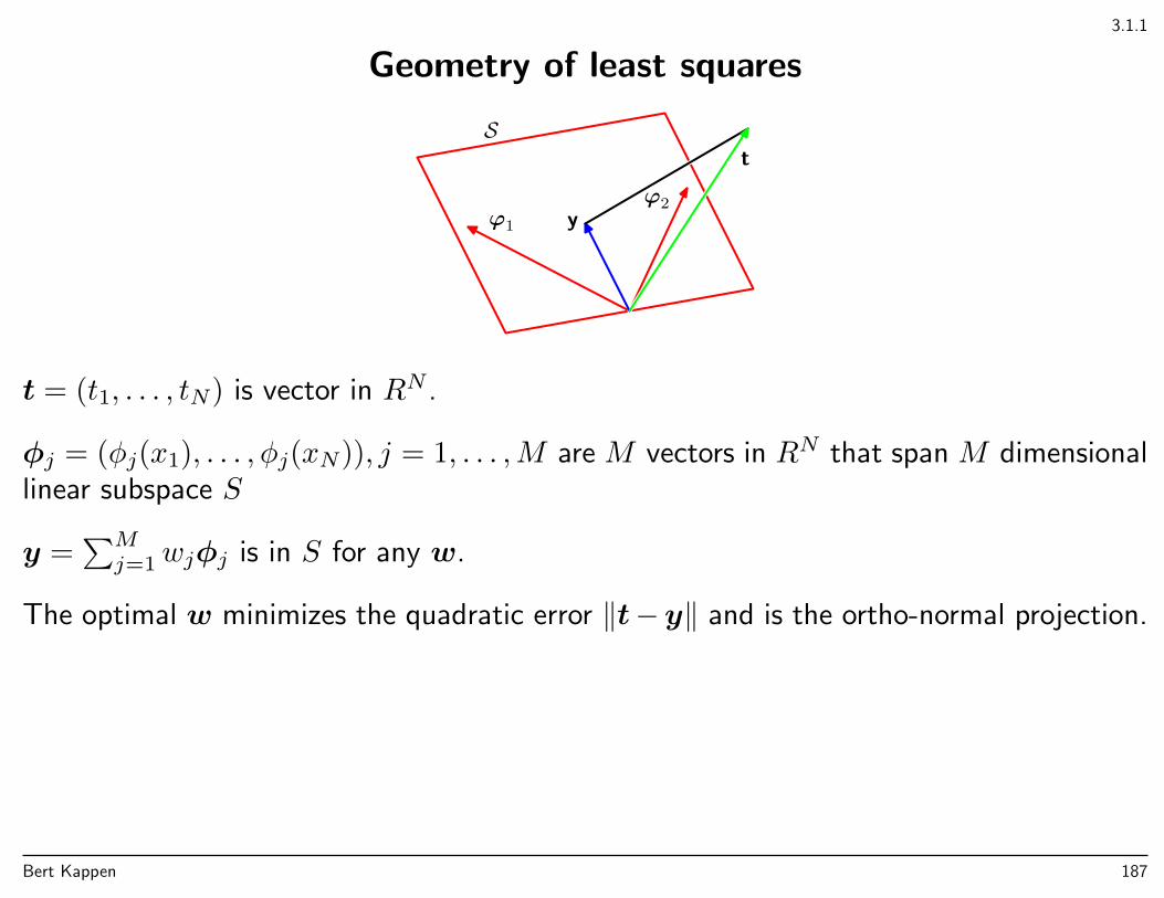
3.1.1
Geometry of least squares
St
yϕ1
ϕ2
t = (t1, . . . , tN) is vector in RN .
φj = (φj(x1), . . . , φj(xN)), j = 1, . . . ,M are M vectors in RN that span M dimensionallinear subspace S
y =∑Mj=1wjφj is in S for any w.
The optimal w minimizes the quadratic error ‖t− y‖ and is the ortho-normal projection.
Bert Kappen 187
3.1.4
Regularized least squares
To avoid overfitting, we can add a regularization term to the log-likelihood, e.g. weightdecay :
ln p(t|X,w, β) + λEW (w) = C − 1
2β
N∑i=1
(tn −wTφ(xn)
)2︸ ︷︷ ︸
sum-of-squares error function
− 1
2λwTw︸ ︷︷ ︸
regularizer
Maximizing with respect to w now gives the following optimum:
w = (λI + ΦTΦ)−1ΦT t
NB: adding the diagonal makes the matrix of maximal rank.
Bert Kappen 188
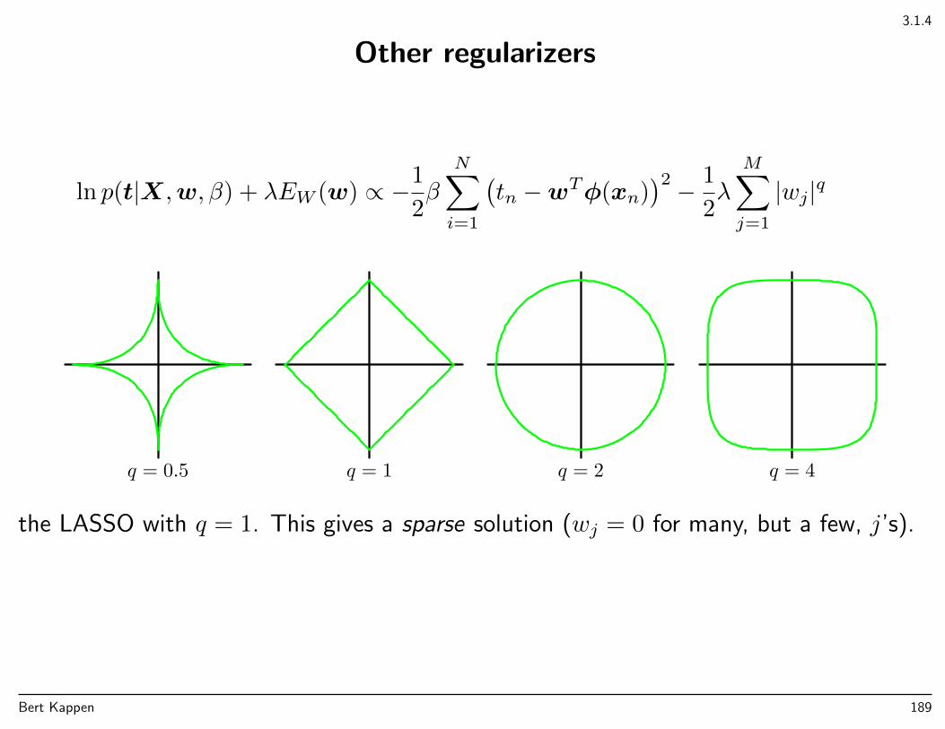
3.1.4
Other regularizers
ln p(t|X,w, β) + λEW (w) ∝ −1
2β
N∑i=1
(tn −wTφ(xn)
)2 − 1
2λ
M∑j=1
|wj|q
q = 0.5 q = 1 q = 2 q = 4
the LASSO with q = 1. This gives a sparse solution (wj = 0 for many, but a few, j’s).
Bert Kappen 189
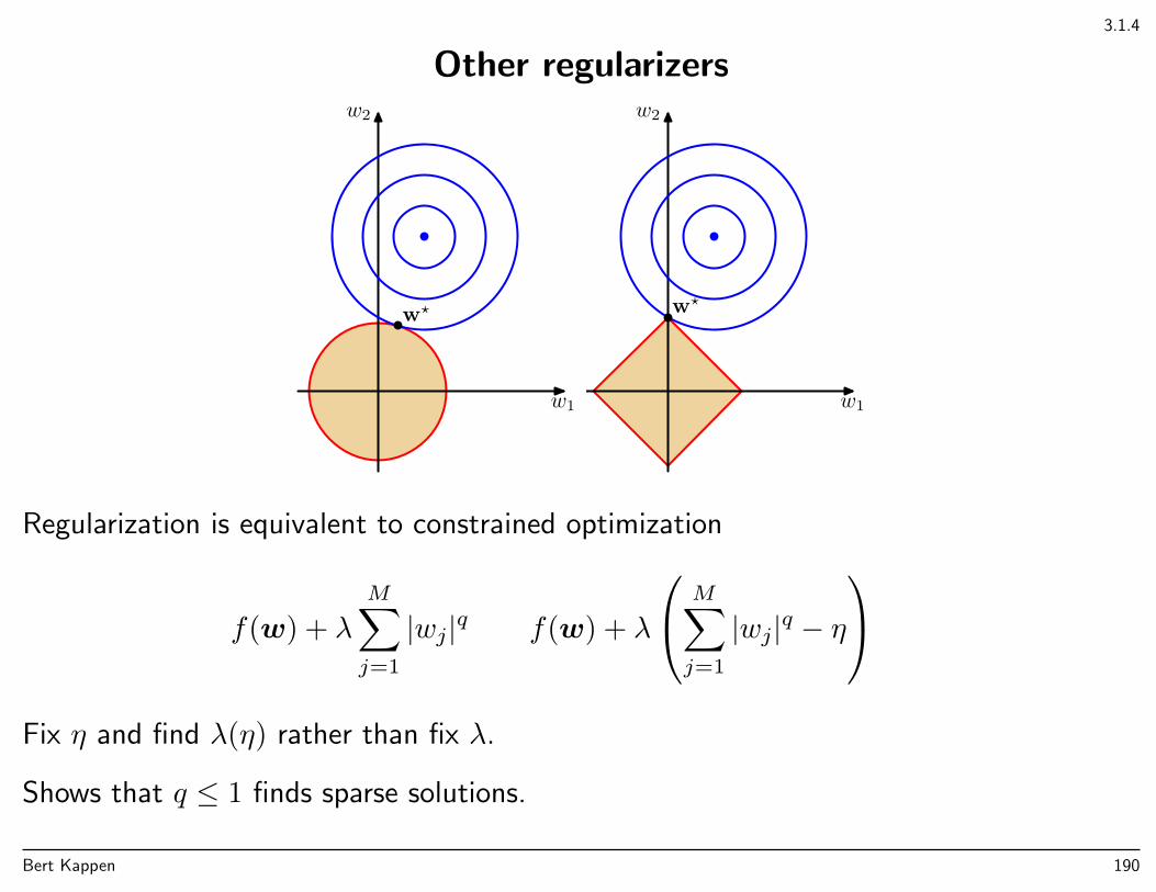
3.1.4
Other regularizers
w1
w2
w?
w1
w2
w?
Regularization is equivalent to constrained optimization
f(w) + λ
M∑j=1
|wj|q f(w) + λ
M∑j=1
|wj|q − η
Fix η and find λ(η) rather than fix λ.
Shows that q ≤ 1 finds sparse solutions.
Bert Kappen 190
3.2
Bias-Variance Decomposition
Complex models tend to overfit. Simple models tend to be too rigid. Number of termsin polynomial, weight decay constant λ.
(Treatment of 1.5.5). Consider a regression problem with squared loss function
E(L) =
∫ (y(x)− t
)2p(x, t)dxdt
p(x, t) is the true underlying model, y(x) is our estimate of t at x.
The optimal y minimizes E(L):
δE(L)
δy(x)= 2
∫ (y(x)− t
)p(x, t)dt = 0
y(x) =
∫tp(x, t)dt
p(x)=
∫tp(t|x)dt = IE(t|x) ≡ h(x)
Bert Kappen 191
1.5.5
Bias-Variance Decomposition
The square loss can also be written as
E(L) =
∫ (y(x)− t
)2p(x, t)dxdt
=
∫ (y(x)− h(x) + h(x)− t
)2p(x, t)dxdt
=
∫ ((y(x)− h(x)
)2+(h(x)− t
)2+ 2
(y(x)− h(x)
)(h(x)− t
))p(x, t)dxdt
=
∫ (y(x)− h(x)
)2p(x)dx+
∫ (t− h(x)
)2p(x, t)dxdt
The first term depends on y and is minimized when y(x) = h(x). The second termis the noise variance in the conditional distribution of t given x, averaged over x:∫
var(t|x)p(x)dx, with var(t|x) =∫dtp(t|x) (t− h(x))
2
We further analyze the first term.
Bert Kappen 192
3.2
Bias-Variance Decomposition
When learning with a finite data set D, the solution y(x|D) that minimizes the quadraticloss depends D.
Consider the thought experiment that a large number of data sets D are given. Then wecan construct the average solution hD(x) = IED(y(x|D)), and
(y(x|D)− h(x)
)2=
(y(x|D)− hD(x)
)2+(hD(x)− h(x)
)2+ 2
(y(x|D)− hD(x)
)(hD(x)− h(x)
)IED(y(x)− h(x)
)2= IED
(y(x|D)− hD(x)
)2︸ ︷︷ ︸variance
+ IED(hD(x)− h(x)
)2︸ ︷︷ ︸bias2
Substitution in expected square loss E(L):
IEDE(L) =
∫IED(y(x)− h(x)
)2p(x)dx+
∫ (t− h(x)
)2p(x, t)dxdt
= bias2 + variance + noise
Bert Kappen 193
3.2
Bias2: difference between average solution IED(y(x|D)) and true solution IE(t|x).Variance: scatter of individual solutions y(x|D) around their mean IED(y(x|D)).Noise: (true) scatter of the data points t around their mean IE(t|x).
Objective is to minimize bias2+variance. Noise cannot be optimized.
Difference models make different trade-off of bias and variance:
• Flexible/complex model: low bias, high variance
• Rigid/simple model: high bias, low variance
Best model strikes the best balance.
Bert Kappen 194
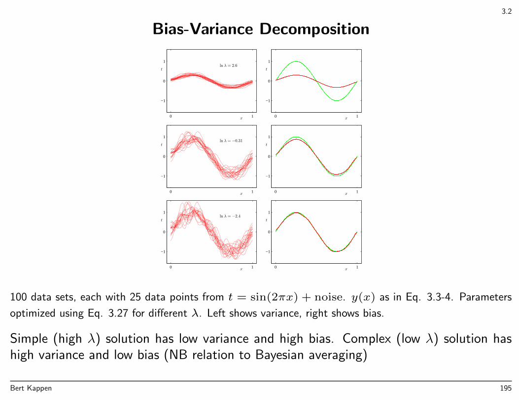
3.2
Bias-Variance Decomposition
x
tln λ = 2.6
0 1
−1
0
1
x
t
0 1
−1
0
1
x
tln λ = −0.31
0 1
−1
0
1
x
t
0 1
−1
0
1
x
tln λ = −2.4
0 1
−1
0
1
x
t
0 1
−1
0
1
100 data sets, each with 25 data points from t = sin(2πx) + noise. y(x) as in Eq. 3.3-4. Parameters
optimized using Eq. 3.27 for different λ. Left shows variance, right shows bias.
Simple (high λ) solution has low variance and high bias. Complex (low λ) solution hashigh variance and low bias (NB relation to Bayesian averaging)
Bert Kappen 195
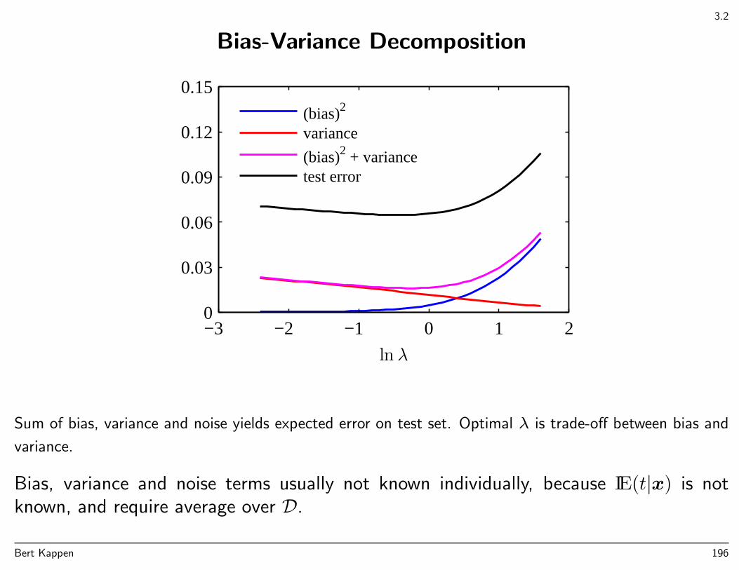
3.2
Bias-Variance Decomposition
ln λ
−3 −2 −1 0 1 20
0.03
0.06
0.09
0.12
0.15
(bias)2
variance
(bias)2 + variancetest error
Sum of bias, variance and noise yields expected error on test set. Optimal λ is trade-off between bias and
variance.
Bias, variance and noise terms usually not known individually, because IE(t|x) is notknown, and require average over D.
Bert Kappen 196
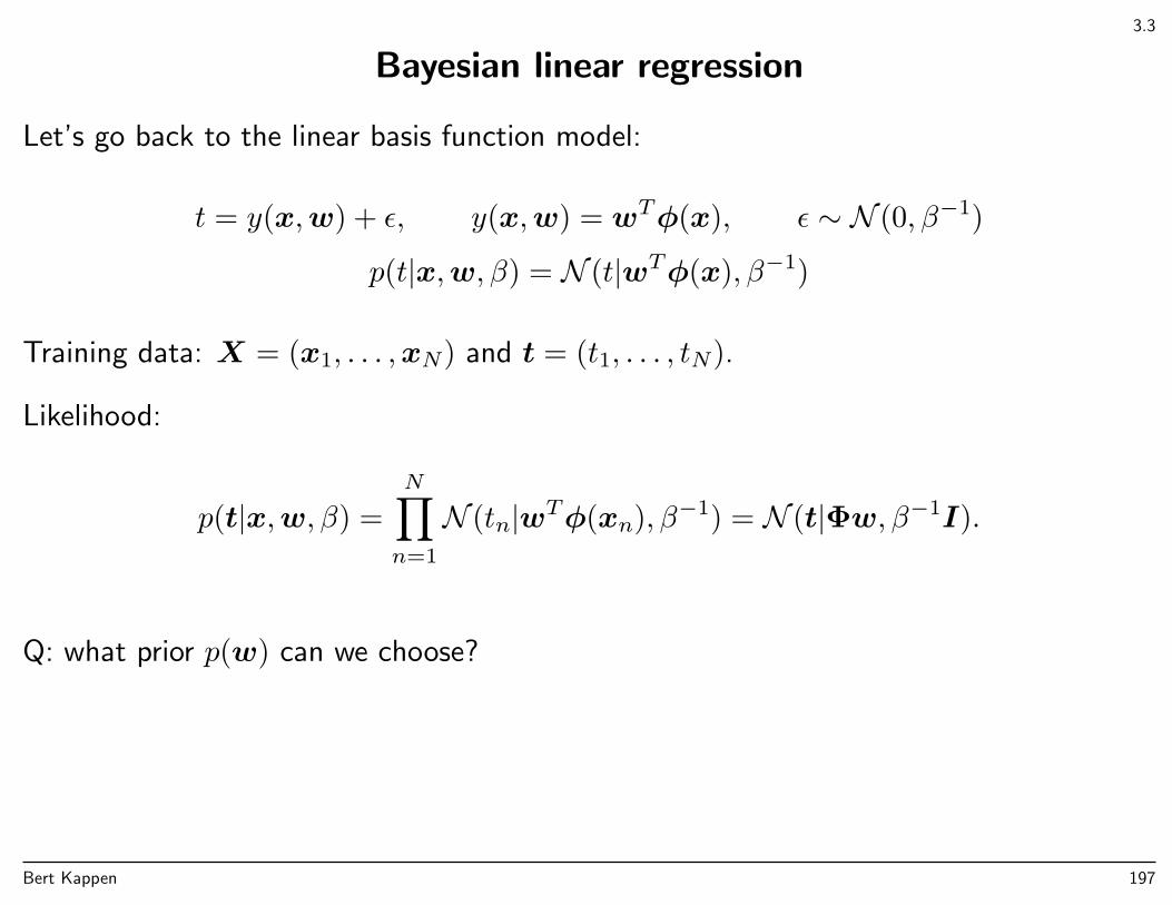
3.3
Bayesian linear regression
Let’s go back to the linear basis function model:
t = y(x,w) + ε, y(x,w) = wTφ(x), ε ∼ N (0, β−1)
p(t|x,w, β) = N (t|wTφ(x), β−1)
Training data: X = (x1, . . . ,xN) and t = (t1, . . . , tN).
Likelihood:
p(t|x,w, β) =
N∏n=1
N (tn|wTφ(xn), β−1) = N (t|Φw, β−1I).
Q: what prior p(w) can we choose?
Bert Kappen 197
3.3
Bayesian linear regression
Let’s go back to the linear basis function model:
t = y(x,w) + ε, y(x,w) = wTφ(x), ε ∼ N (0, β−1)
p(t|x,w, β) = N (t|wTφ(x), β−1)
Training data: X = (x1, . . . ,xN) and t = (t1, . . . , tN).
Likelihood:
p(t|x,w, β) =
N∏n=1
N (tn|wTφ(xn), β−1) = N (t|Φw, β−1I).
Q: what prior p(w) can we choose?A: We make life easy by choosing a conjugate prior, which is a Gaussian
p(w) = N (w|m0, S0)
Bert Kappen 198
3.3
Bayesian linear regression
Then, the posterior will also be Gaussian. Prior and likelihood:
p(w) = N (w|m0, S0)
p(t|w) = N (t|Φw, β−1I)
Then, by applying 2.113 + 2.114⇒ 2.116, we get the posterior:
p(w|t) = . . .?
Bert Kappen 199
3.3
Bayesian linear regression
Then, the posterior will also be Gaussian. Prior and likelihood:
p(w) = N (w|m0, S0)
p(t|w) = N (t|Φw, β−1I)
Then, by applying 2.113 + 2.114⇒ 2.116, we get the posterior:
p(w|t) = N (w|mN , SN)
with
mN = SN(S−10 m0 + βΦT t)
S−1N = S−1
0 + βΦTΦ
Since posterior is Gaussian, its mode is mN .
When S−10 → 0 (broad prior) mN → β(ΦTΦ)−1ΦT t which is the ML solution.
ΦTΦ ∝ N . Therefore SN → 0 when N large.
Bert Kappen 200
3.3
Details
Correspondence with (2.113-114):
p(x) = N (x|µ,Λ−1) p(w) = N (w|m0, S0)
p(y|x) = N (y|Ax+ b,L−1) p(t|w) = N (t|Φw, β−1I)
µ = m0,Λ−1 = S0,A = Φ, b = 0,L = βI.
Thus from (2.116), posterior p(w|t) = N (w|mN , SN) with
mN = SN(βΦT t+ S−10 m0)
S−1N = S−1
0 + βΦTΦ
Bert Kappen 201
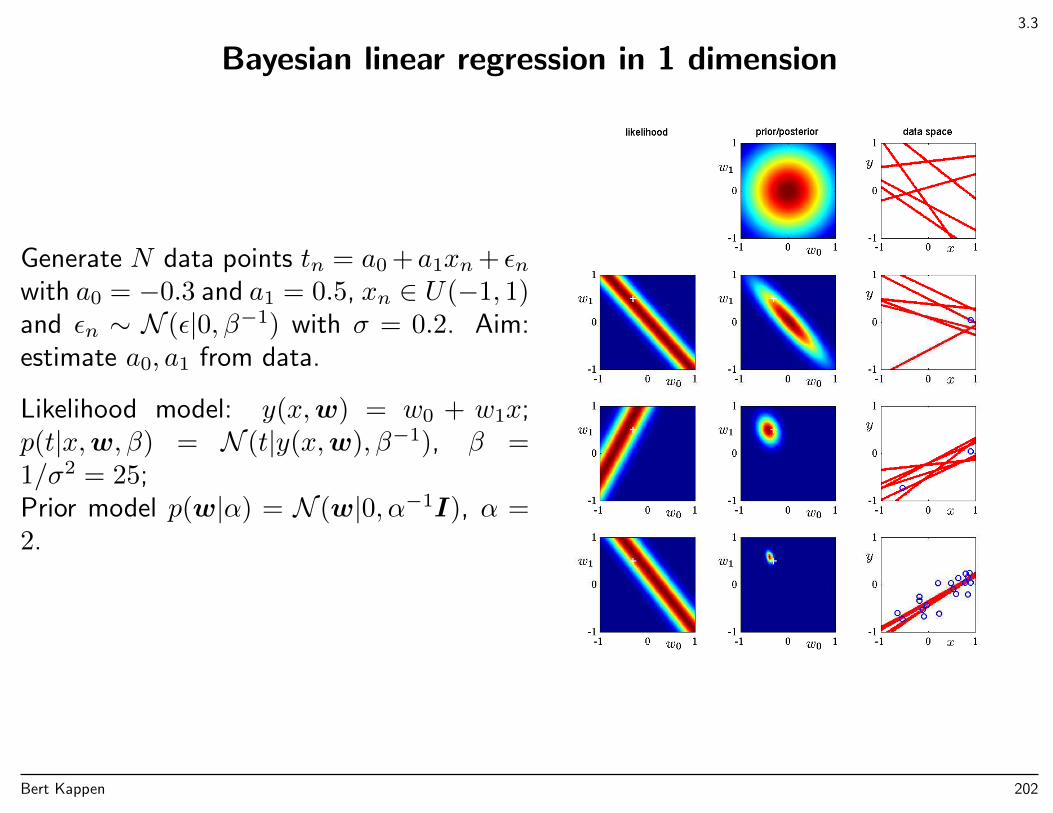
3.3
Bayesian linear regression in 1 dimension
Generate N data points tn = a0 + a1xn+ εnwith a0 = −0.3 and a1 = 0.5, xn ∈ U(−1, 1)and εn ∼ N (ε|0, β−1) with σ = 0.2. Aim:estimate a0, a1 from data.
Likelihood model: y(x,w) = w0 + w1x;p(t|x,w, β) = N (t|y(x,w), β−1), β =1/σ2 = 25;Prior model p(w|α) = N (w|0, α−1I), α =2.
Bert Kappen 202
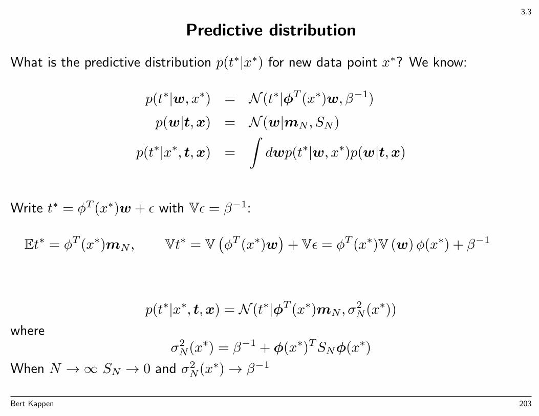
3.3
Predictive distribution
What is the predictive distribution p(t∗|x∗) for new data point x∗? We know:
p(t∗|w, x∗) = N (t∗|φT (x∗)w, β−1)
p(w|t,x) = N (w|mN , SN)
p(t∗|x∗, t,x) =
∫dwp(t∗|w, x∗)p(w|t,x)
Write t∗ = φT (x∗)w + ε with Vε = β−1:
Et∗ = φT (x∗)mN , Vt∗ = V(φT (x∗)w
)+ Vε = φT (x∗)V (w)φ(x∗) + β−1
p(t∗|x∗, t,x) = N (t∗|φT (x∗)mN , σ2N(x∗))
whereσ2N(x∗) = β−1 + φ(x∗)TSNφ(x∗)
When N →∞ SN → 0 and σ2N(x∗)→ β−1
Bert Kappen 203

3.3
Predictive distribution
Mean prediction is t∗ =∑j φj(x
∗)(mN)j depends on input x∗ and ’training data’ x, t:(Φnj = φj(xn)):
S−1N = S−1
0 + β∑n
φ(xn)φ(xn)T
(mN)j =∑j′
(SN)jj′
β∑n
φj′(xn)tn +∑j′′
(S−1
0
)j′j′′
(m0)j′′
variance
σ2N(x∗) = β−1 + φ(x∗)TSNφ(x∗)
goes to zero for x∗ in areas where no basis functions, ie. over confident. This negativefeature can be resolved using Gaussian processes (section 6.4).
Bert Kappen 204
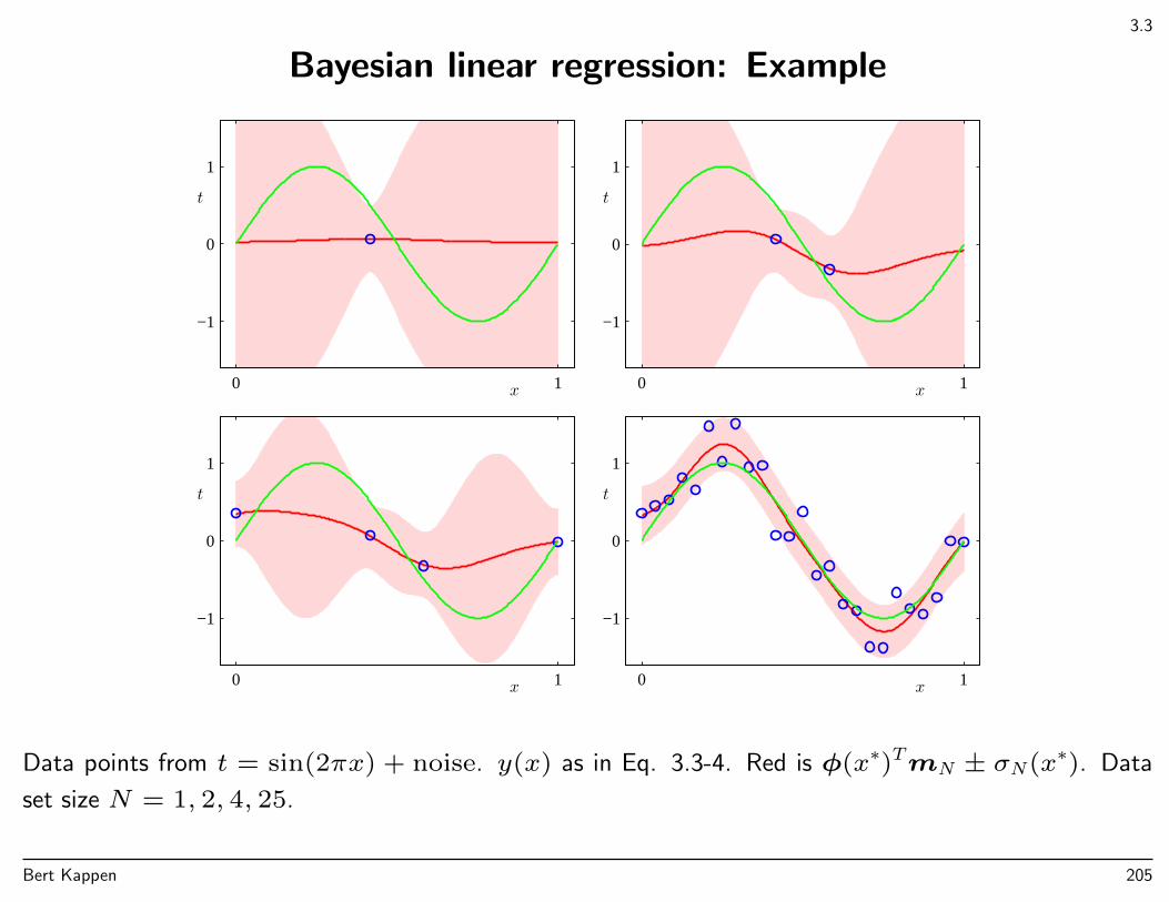
3.3
Bayesian linear regression: Example
x
t
0 1
−1
0
1
x
t
0 1
−1
0
1
x
t
0 1
−1
0
1
x
t
0 1
−1
0
1
Data points from t = sin(2πx) + noise. y(x) as in Eq. 3.3-4. Red is φ(x∗)TmN ± σN(x∗). Data
set size N = 1, 2, 4, 25.
Bert Kappen 205
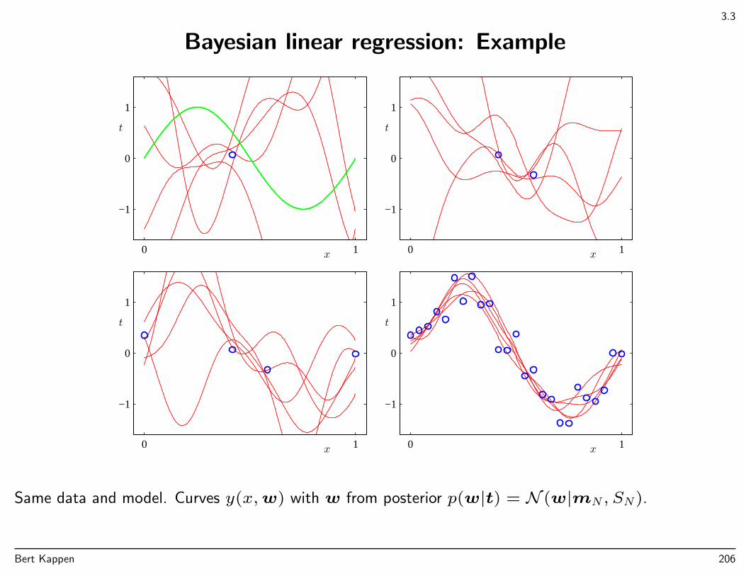
3.3
Bayesian linear regression: Example
x
t
0 1
−1
0
1
x
t
0 1
−1
0
1
x
t
0 1
−1
0
1
x
t
0 1
−1
0
1
Same data and model. Curves y(x,w) with w from posterior p(w|t) = N (w|mN , SN).
Bert Kappen 206
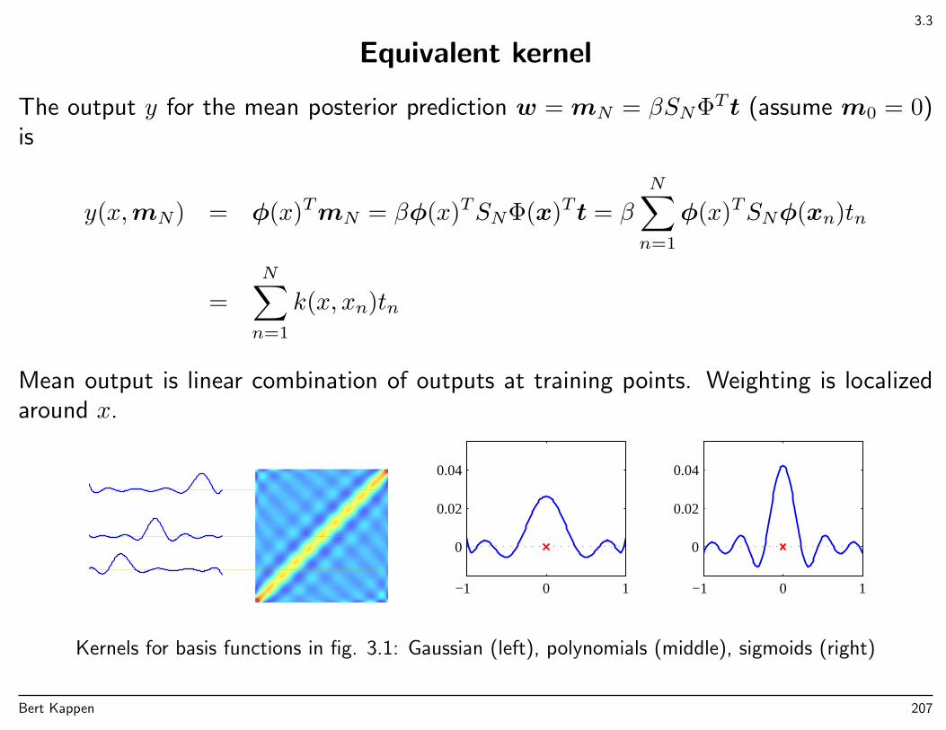
3.3
Equivalent kernel
The output y for the mean posterior prediction w = mN = βSNΦT t (assume m0 = 0)is
y(x,mN) = φ(x)TmN = βφ(x)TSNΦ(x)T t = β
N∑n=1
φ(x)TSNφ(xn)tn
=
N∑n=1
k(x, xn)tn
Mean output is linear combination of outputs at training points. Weighting is localizedaround x.
−1 0 1
0
0.02
0.04
−1 0 1
0
0.02
0.04
Kernels for basis functions in fig. 3.1: Gaussian (left), polynomials (middle), sigmoids (right)
Bert Kappen 207
3.3
Equivalent kernel
The outputs at two different inputs are correlated:
Cov (y(x), y(x′)) = Cov(φ(x)Tw,wTφ(x′)) = φ(x)TVwφ(x′) = φ(x)TSNφ(x′)
= β−1k(x, x′)
Nearby points are highly correlated, and distant points are uncorrelated.
One can specify a regression problem in terms of a kernel directly instead of a linearcombination of basis functions (chapter 6).
Bert Kappen 208
3.4
Bayesian model comparison
Maximum likelihood suffers from overfitting, which requires testing models of differentcomplexity on separate data.
Bayesian approach allows to compare different models directly on the training data, butrequires integration over model parameters.
Consider L probability models and a set of data generated from one of these models. Wedefine a prior over models p(Mi), i = 1, . . . , L to express our prior uncertainty.
Given the training data D, we wish to compute the posterior probability
p(Mi|D) ∝ p(D|Mi)p(Mi)
p(D|Mi) is called model evidence, also marginal likelihood, since it integrates over modelparameters:
p(D|Mi) =
∫p(D|w,Mi)p(w|Mi)dw
Bert Kappen 209
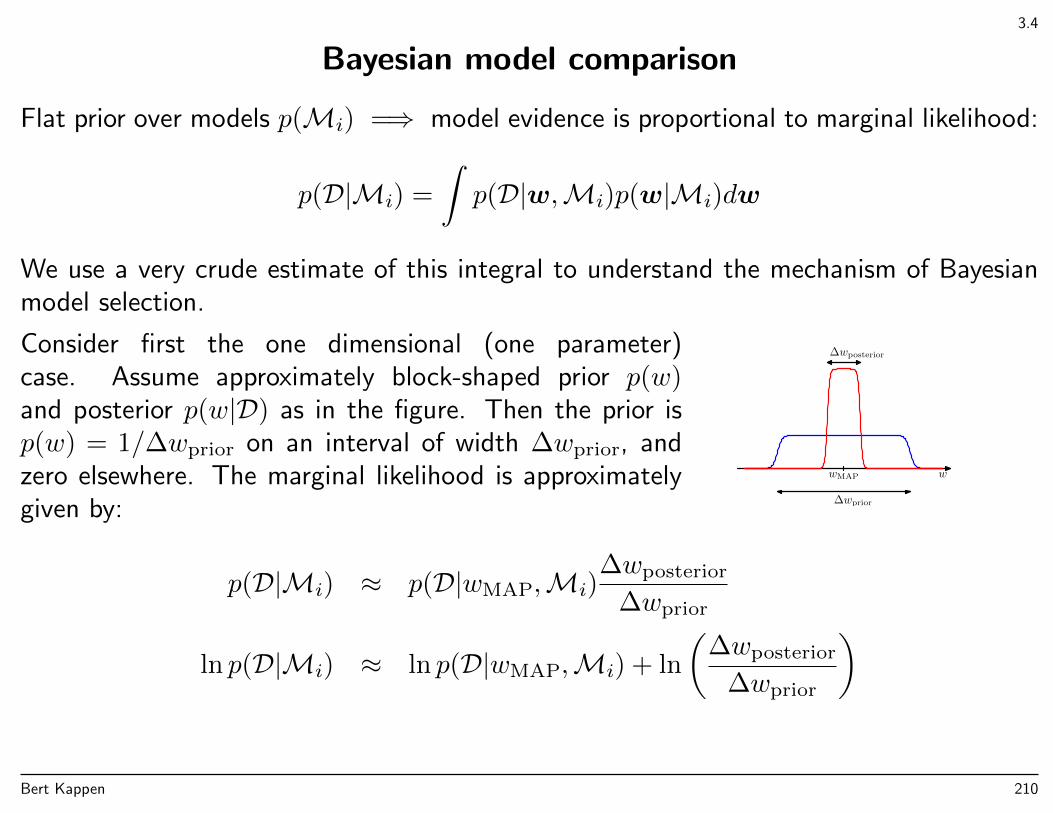
3.4
Bayesian model comparison
Flat prior over models p(Mi) =⇒ model evidence is proportional to marginal likelihood:
p(D|Mi) =
∫p(D|w,Mi)p(w|Mi)dw
We use a very crude estimate of this integral to understand the mechanism of Bayesianmodel selection.
Consider first the one dimensional (one parameter)case. Assume approximately block-shaped prior p(w)and posterior p(w|D) as in the figure. Then the prior isp(w) = 1/∆wprior on an interval of width ∆wprior, andzero elsewhere. The marginal likelihood is approximatelygiven by:
∆wposterior
∆wprior
wMAP w
p(D|Mi) ≈ p(D|wMAP,Mi)∆wposterior
∆wprior
ln p(D|Mi) ≈ ln p(D|wMAP,Mi) + ln
(∆wposterior
∆wprior
)
Bert Kappen 210
3.4
Bayesian model comparison
The Bayesian integration gives a negative correction to the ML estimate.
With M model parameters, the same argument gives
ln p(D|Mi) ≈ ln p(D|wMAP,Mi) +M ln
(∆wposterior
∆wprior
)With increasing M , the first term increases (better fit), but the second term decreases.
Bert Kappen 211
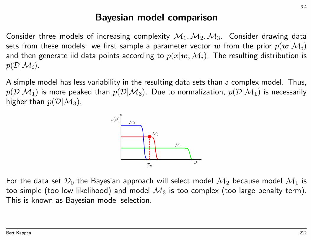
3.4
Bayesian model comparison
Consider three models of increasing complexity M1,M2,M3. Consider drawing datasets from these models: we first sample a parameter vector w from the prior p(w|Mi)and then generate iid data points according to p(x|w,Mi). The resulting distribution isp(D|Mi).
A simple model has less variability in the resulting data sets than a complex model. Thus,p(D|M1) is more peaked than p(D|M3). Due to normalization, p(D|M1) is necessarilyhigher than p(D|M3).
p(D)
DD0
M1
M2
M3
For the data set D0 the Bayesian approach will select model M2 because model M1 istoo simple (too low likelihood) and model M3 is too complex (too large penalty term).This is known as Bayesian model selection.
Bert Kappen 212

3.5.1
Evidence framework
The Bayesian linear regression approach assume a prior (3.48)
p(w|α,M) =( α
2π
)M/2
exp(−α
2wTw
)and a likelihood (3.10)
p(t|w, β,M) =
(β
2π
)N/2exp
(−β
2‖t− Φw‖2
).
The marginal likelihood is
p(t|α, β,M) =
∫dwp(w|α,M)p(t|w, β,M)
=( α
2π
)M/2(β
2π
)N/2 ∫dw exp(−E(w))
Bert Kappen 213
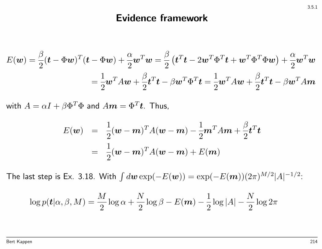
3.5.1
Evidence framework
E(w) =β
2(t− Φw)T (t− Φw) +
α
2wTw =
β
2
(tT t− 2wTΦT t+wTΦTΦw
)+α
2wTw
=1
2wTAw +
β
2tT t− βwTΦT t =
1
2wTAw +
β
2tT t− βwTAm
with A = αI + βΦTΦ and Am = ΦT t. Thus,
E(w) =1
2(w −m)TA(w −m)− 1
2mTAm+
β
2tT t
=1
2(w −m)TA(w −m) + E(m)
The last step is Ex. 3.18. With∫dw exp(−E(w)) = exp(−E(m))(2π)M/2|A|−1/2:
log p(t|α, β,M) =M
2logα+
N
2log β − E(m)− 1
2log |A| − N
2log 2π
Bert Kappen 214
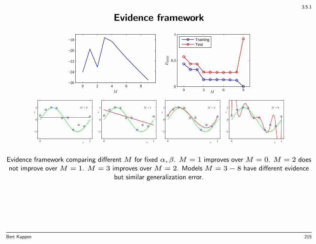
3.5.1
Evidence framework
M
0 2 4 6 8−26
−24
−22
−20
−18
M
ERMS
0 3 6 90
0.5
1TrainingTest
x
t
M = 0
0 1
−1
0
1
x
t
M = 1
0 1
−1
0
1
x
t
M = 3
0 1
−1
0
1
x
t
M = 9
0 1
−1
0
1
Evidence framework comparing different M for fixed α, β. M = 1 improves over M = 0. M = 2 does
not improve over M = 1. M = 3 improves over M = 2. Models M = 3− 8 have different evidence
but similar generalization error.
Bert Kappen 215
Handout Perceptrons
The Perceptron
Relevant in history of pattern recognition and neural networks.
• Perceptron learning rule + convergence, Rosenblatt (1962)
• Perceptron critique (Minsky and Papert, 1969) → ”Dark ages of neural networks”
• Revival in the 80’s: Backpropagation
Bert Kappen 216
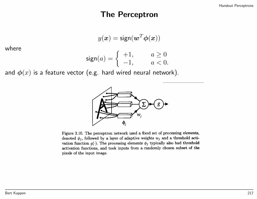
Handout Perceptrons
The Perceptron
y(x) = sign(wTφ(x))
where
sign(a) =
+1, a ≥ 0−1, a < 0.
and φ(x) is a feature vector (e.g. hard wired neural network).
Bert Kappen 217

Handout Perceptrons
Threshold units
Consider the simplest case of binary threshold neurons:
g(h) = sign(h)
Then, the learning condition becomes
sign(w · ξµ) = ζµ, µ = 1, . . . , P
Since ζµ = ±1, we have
sign(w · ξµζµ) = 1 or w · xµ > 0
with xµj = ξµj ζµ.
Bert Kappen 218

Handout Perceptrons
Linear separation
Classification depends on sign of w · ξ. Thus, decision boundary is hyper plane:
0 = w · ξ =
n∑j=1
wjξj − θ
Perceptron can solve linearly separable problems.
AND problem is linearly separable.
XOR problem and linearly dependent inputs not linearly separable.
Bert Kappen 219
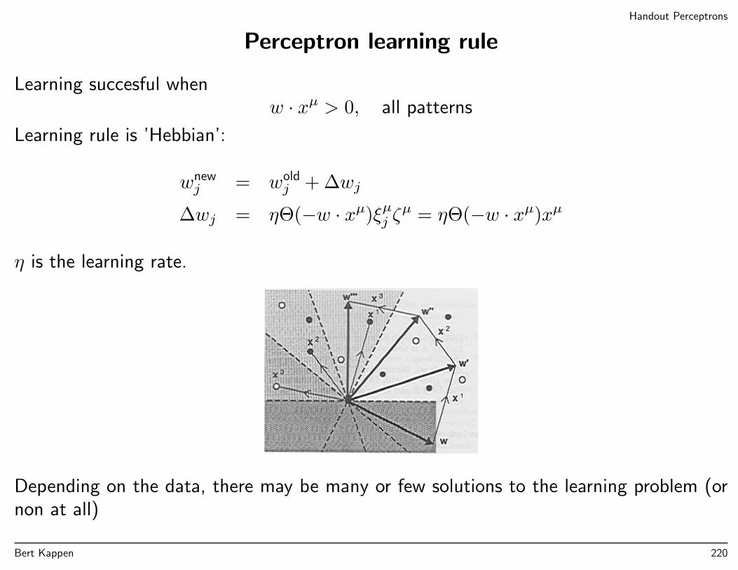
Handout Perceptrons
Perceptron learning rule
Learning succesful whenw · xµ > 0, all patterns
Learning rule is ’Hebbian’:
wnewj = wold
j + ∆wj
∆wj = ηΘ(−w · xµ)ξµj ζµ = ηΘ(−w · xµ)xµ
η is the learning rate.
Depending on the data, there may be many or few solutions to the learning problem (ornon at all)
Bert Kappen 220
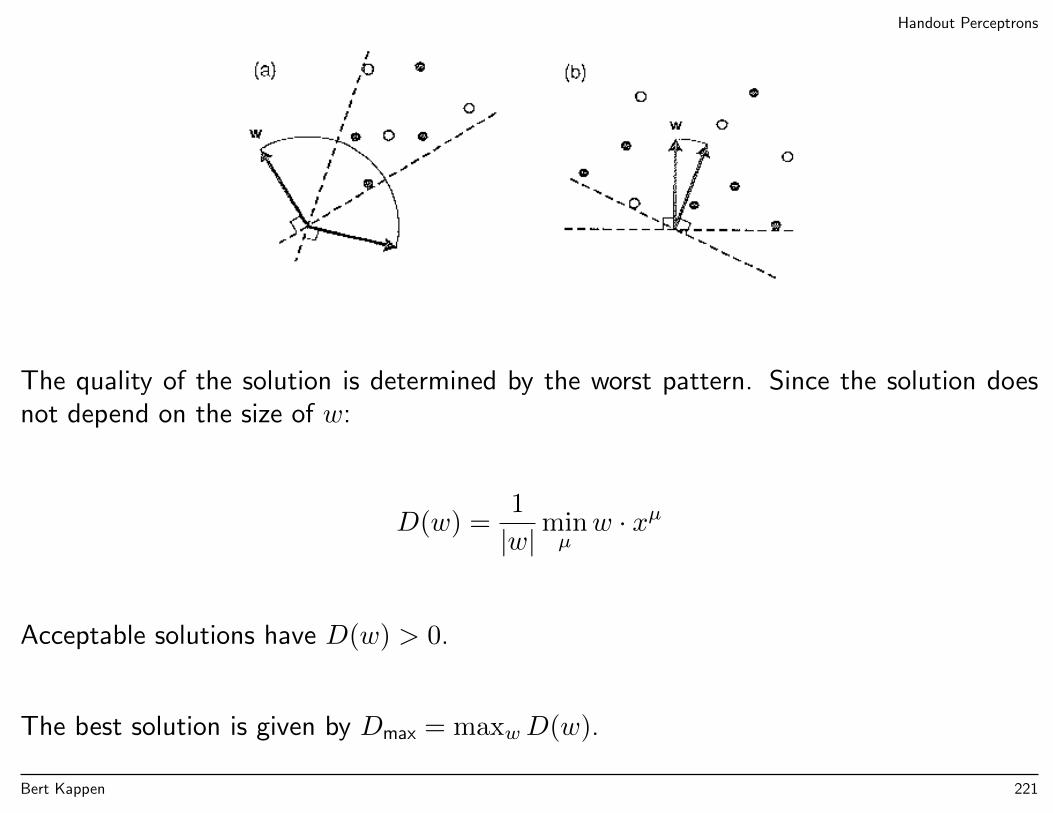
Handout Perceptrons
The quality of the solution is determined by the worst pattern. Since the solution doesnot depend on the size of w:
D(w) =1
|w|minµw · xµ
Acceptable solutions have D(w) > 0.
The best solution is given by Dmax = maxwD(w).
Bert Kappen 221
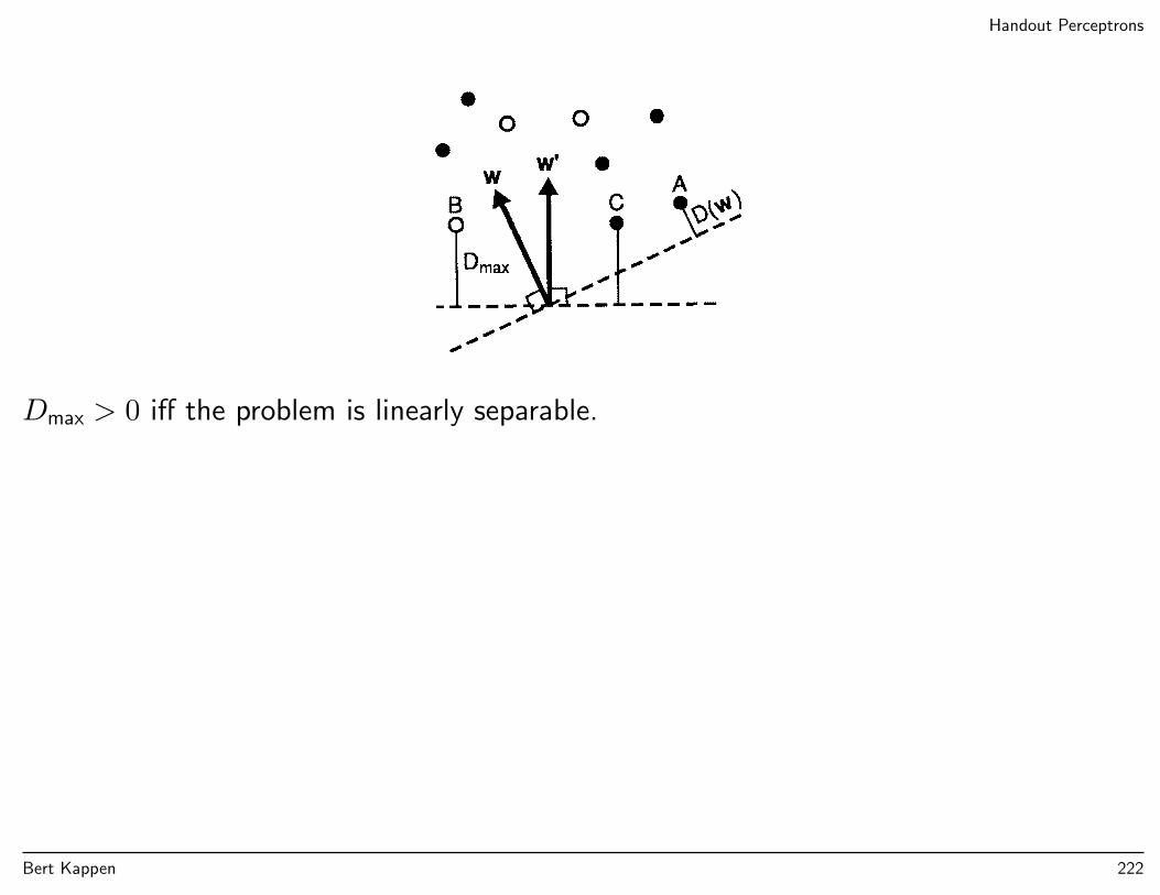
Handout Perceptrons
Dmax > 0 iff the problem is linearly separable.
Bert Kappen 222
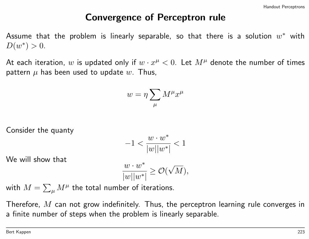
Handout Perceptrons
Convergence of Perceptron rule
Assume that the problem is linearly separable, so that there is a solution w∗ withD(w∗) > 0.
At each iteration, w is updated only if w · xµ < 0. Let Mµ denote the number of timespattern µ has been used to update w. Thus,
w = η∑µ
Mµxµ
Consider the quanty
−1 <w · w∗|w||w∗| < 1
We will show thatw · w∗|w||w∗| ≥ O(
√M),
with M =∑µM
µ the total number of iterations.
Therefore, M can not grow indefinitely. Thus, the perceptron learning rule converges ina finite number of steps when the problem is linearly separable.
Bert Kappen 223
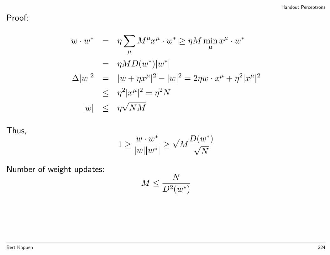
Handout Perceptrons
Proof:
w · w∗ = η∑µ
Mµxµ · w∗ ≥ ηM minµxµ · w∗
= ηMD(w∗)|w∗|∆|w|2 = |w + ηxµ|2 − |w|2 = 2ηw · xµ + η2|xµ|2
≤ η2|xµ|2 = η2N
|w| ≤ η√NM
Thus,
1 ≥ w · w∗|w||w∗| ≥
√MD(w∗)√
N
Number of weight updates:
M ≤ N
D2(w∗)
Bert Kappen 224
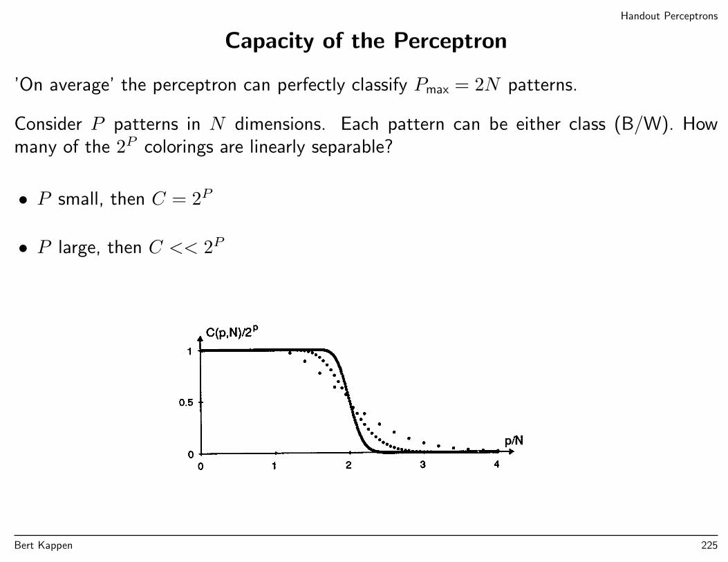
Handout Perceptrons
Capacity of the Perceptron
’On average’ the perceptron can perfectly classify Pmax = 2N patterns.
Consider P patterns in N dimensions. Each pattern can be either class (B/W). Howmany of the 2P colorings are linearly separable?
• P small, then C = 2P
• P large, then C << 2P
Bert Kappen 225
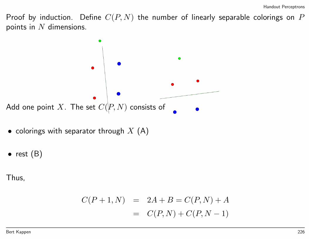
Handout Perceptrons
Proof by induction. Define C(P,N) the number of linearly separable colorings on Ppoints in N dimensions.
Add one point X. The set C(P,N) consists of
• colorings with separator through X (A)
• rest (B)
Thus,
C(P + 1, N) = 2A+B = C(P,N) +A
= C(P,N) + C(P,N − 1)
Bert Kappen 226

Handout Perceptrons
Yields7
C(P,N) = 2
N∑i=0
(P − 1i
)
7NB Error in HKP (∑N−1i=0 ).
Bert Kappen 227
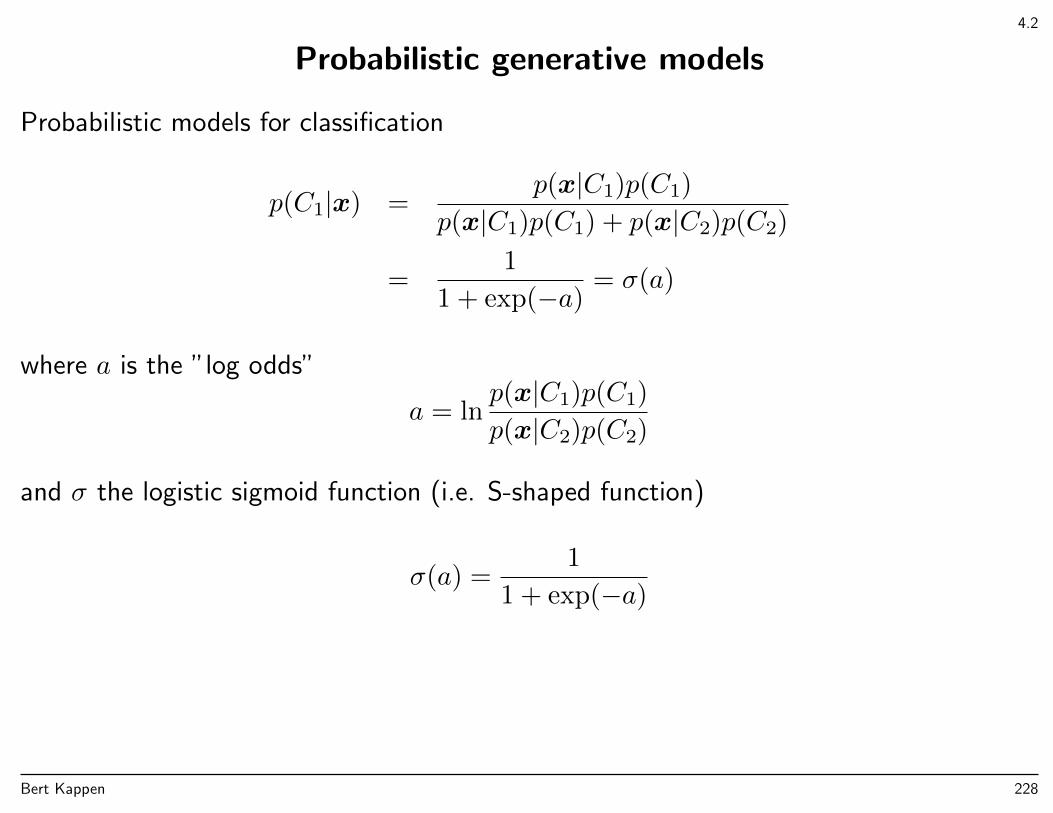
4.2
Probabilistic generative models
Probabilistic models for classification
p(C1|x) =p(x|C1)p(C1)
p(x|C1)p(C1) + p(x|C2)p(C2)
=1
1 + exp(−a)= σ(a)
where a is the ”log odds”
a = lnp(x|C1)p(C1)
p(x|C2)p(C2)
and σ the logistic sigmoid function (i.e. S-shaped function)
σ(a) =1
1 + exp(−a)
Bert Kappen 228
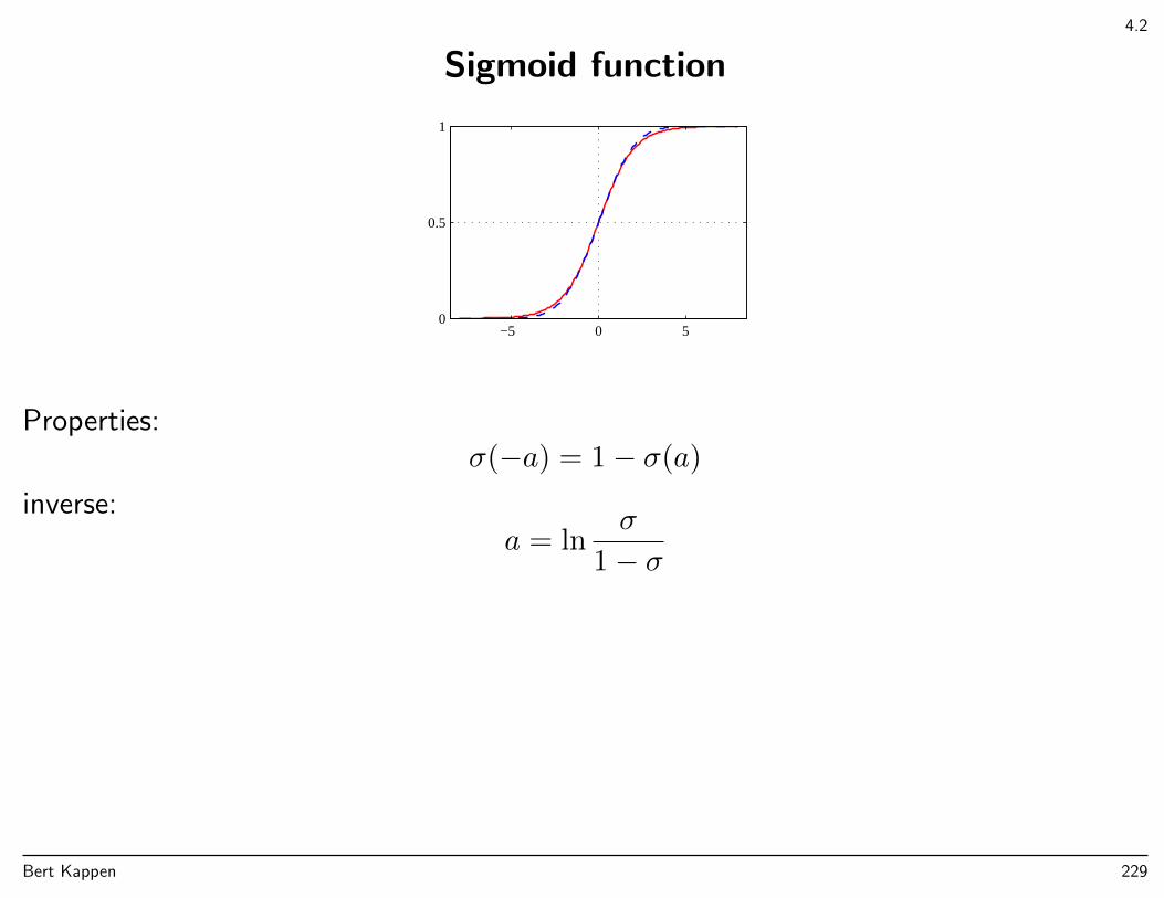
4.2
Sigmoid function
−5 0 50
0.5
1
Properties:σ(−a) = 1− σ(a)
inverse:a = ln
σ
1− σ
Bert Kappen 229
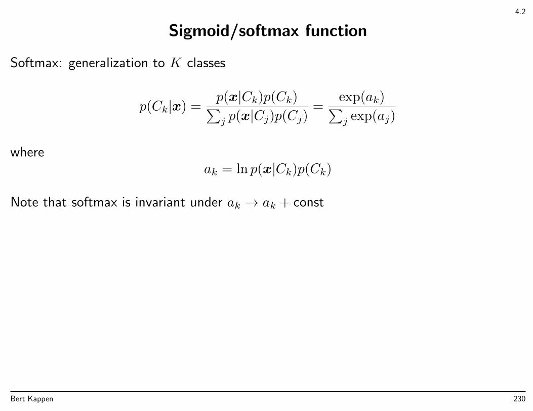
4.2
Sigmoid/softmax function
Softmax: generalization to K classes
p(Ck|x) =p(x|Ck)p(Ck)∑j p(x|Cj)p(Cj)
=exp(ak)∑j exp(aj)
whereak = ln p(x|Ck)p(Ck)
Note that softmax is invariant under ak → ak + const
Bert Kappen 230
4.2.1
Continuous inputs
The discriminant function for a Gaussian distribution is
ak(x) = log p(x|Ck) + log p(Ck)
= −1
2(x− µk)TΣ−1
k (x− µk)−1
2log |Σk|+ log p(Ck)
The decision boundaries ak(x) = al(x) are quadratic functions in d dimensions.
If Σ−1k = Σ−1, then
ak(x) = −1
2xΣ−1x+
1
2µTkΣ−1x+
1
2xΣ−1µk −
1
2µTkΣ−1µk −
1
2log |Σ|+ log p(Ck)
= wTk x+ wk0 + const
with
wTk = µTkΣ−1, wk0 = −1
2µTkΣ−1µk + log p(Ck)
The discriminant function is linear, and the decision boundary is a straight line (orhyper-plane in d dimensions).
Bert Kappen 231
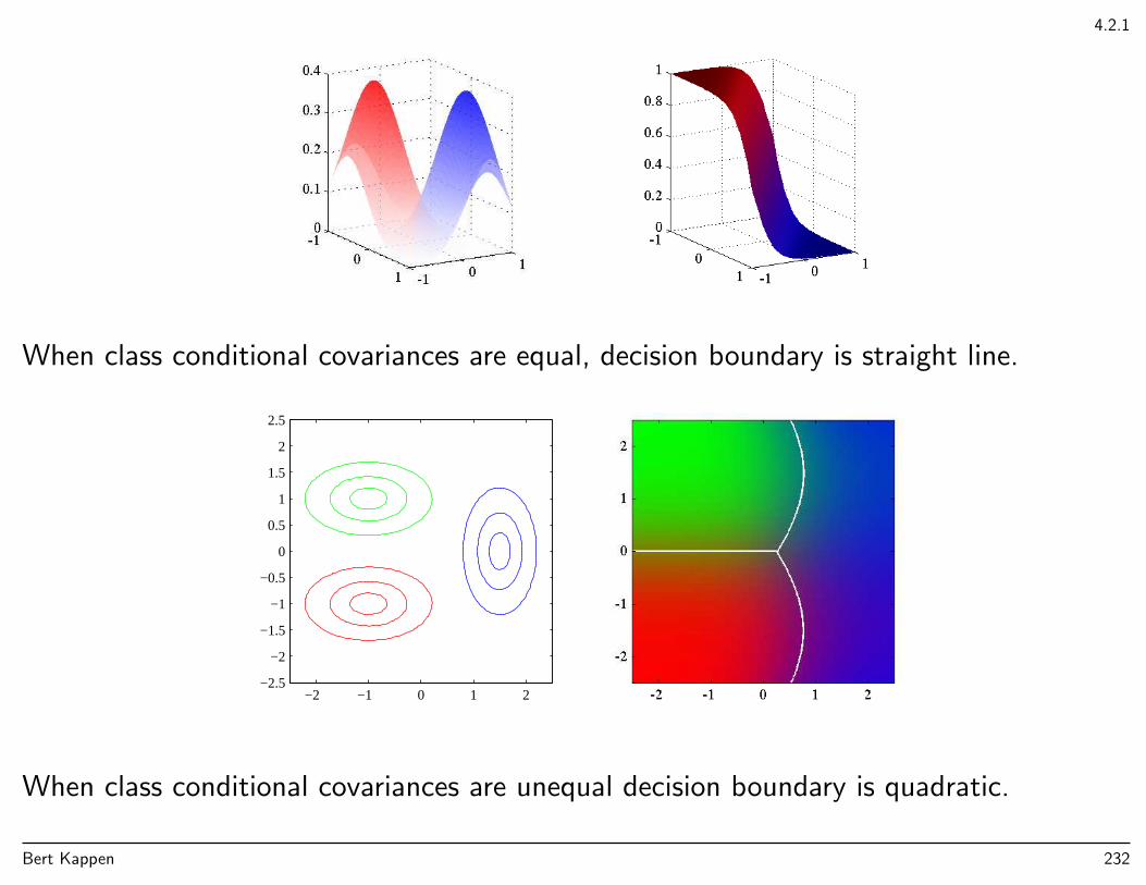
4.2.1
When class conditional covariances are equal, decision boundary is straight line.
−2 −1 0 1 2−2.5
−2
−1.5
−1
−0.5
0
0.5
1
1.5
2
2.5
When class conditional covariances are unequal decision boundary is quadratic.
Bert Kappen 232
4.2.2
Maximum likelihood solution
Once we have specified a parametric functional form for p(x|Ck) and p(Ck) we candetermine parameters using maximum (joint!) likelihood (as usual !).
Actually, for classification, we should aim for the conditional likelihood, but the jointlikelihood is in general easier. In a perfect model, it makes no difference, but withimperfect models, it certainly does!
Example of joint ML: a binary problem with Gaussian class-conditionals, with a sharedcovariance matrix. Data is xn, tnn with labels coded as t = 1, 0 for classes C1, C2.
Class probabilities are parametrized as
p(C1) = π, p(C2) = 1− π
and class-conditional densities as
p(xn|C1) = N (xn|µ1,Σ), p(xn|C2) = N (xn|µ2,Σ)
Bert Kappen 233
4.2.2
Then the likelihood is given by
L = p(t1,x1, . . . , tN ,xn|π,µ1,µ2,Σ) =∏n
p(tn,xn|π,µ1,µ2,Σ)
=∏n
[πN (xn|µ1,Σ)]tn[(1− π)N (xn|µ2,Σ)]1−tn
logL =∑n
tn log[πN (xn|µ1,Σ)] + (1− tn) log[(1− π)N (xn|µ2,Σ)]
The maximum likelihood solution for π and µ1,2:
∂ logL
∂π=
1
π
∑n
tn −1
1− π∑n
(1− tn) π =N1
NN1 =
∑n
tn
∂ logL
∂µ1=
∑n
tn∂ logN (xn|µ1,Σ)
∂µ1= Σ−1
∑n
tn(xn − µ1) µ1 =1
N
∑n
tnxn
∂ logL
∂µ2= . . . µ2 =
1
N
∑n
(1− tn)xn
The maximum likelihood solution for Σ given by Eqs. 4.78-80 (exercise).
Bert Kappen 234
4.3
Probabilistic discriminative models
Discriminative versus generative models
Discriminative models:
• no spoiled effort in modeling joint probabilities. Aims directly at the conditionalprobabilities of interest
• usually fewer parameters
• improved performance when class-conditional p(x|C) assumptions are poor (with jointML).
• basis functions can be employed
Bert Kappen 235
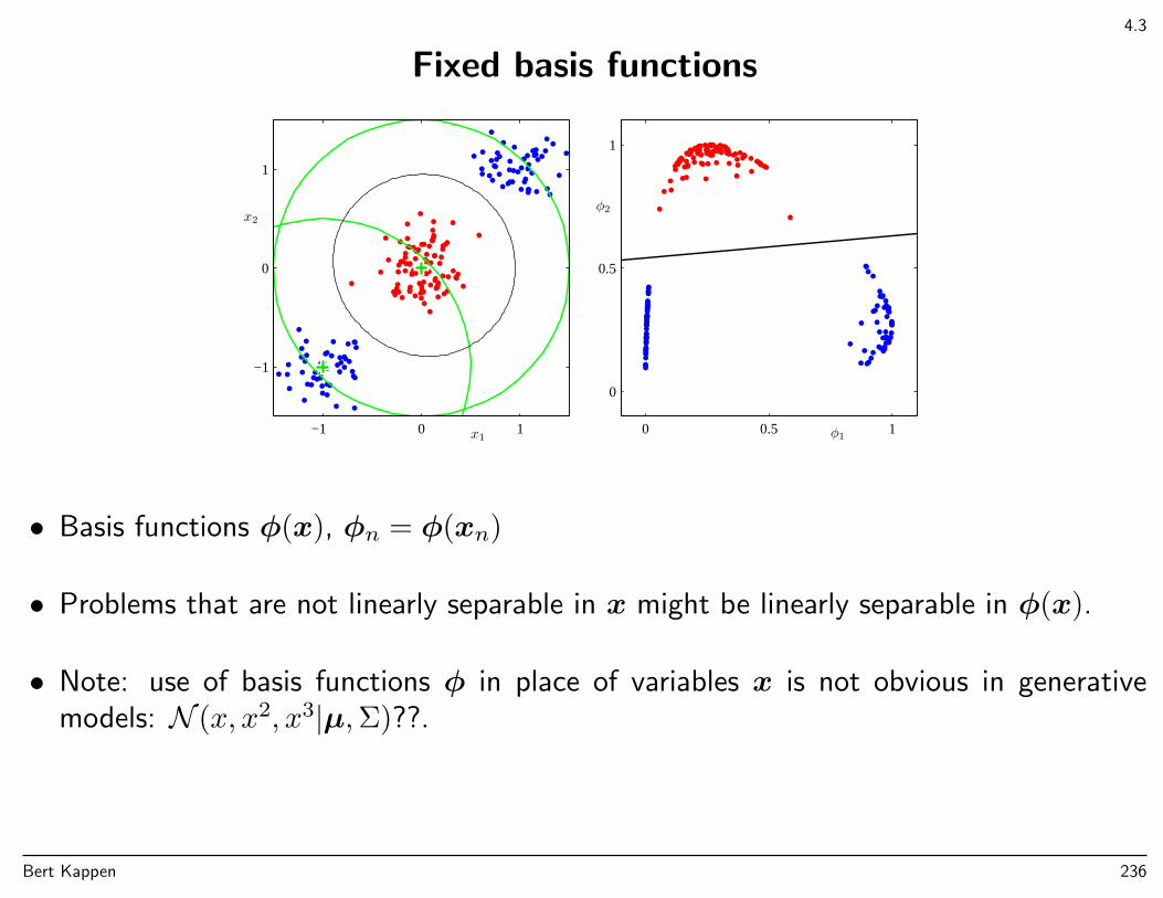
4.3
Fixed basis functions
x1
x2
−1 0 1
−1
0
1
φ1
φ2
0 0.5 1
0
0.5
1
• Basis functions φ(x), φn = φ(xn)
• Problems that are not linearly separable in x might be linearly separable in φ(x).
• Note: use of basis functions φ in place of variables x is not obvious in generativemodels: N (x, x2, x3|µ,Σ)??.
Bert Kappen 236
4.3
Logistic regression
Two class classificationp(C1|φ) = σ(wTφ)
M dimensional feature space: M parameters, while Gaussian class conditional densitieswould require 2M (two means) and M(M+1)/2 (common covariance matrix) parameters.
Maximum likelihood to determine parameters w, (nb. tn ∈ 0, 1)
p(t1, . . . , tN |w, x1, . . . , xN) =∏n
σ(wTφn)tn[1− σ(wTφn)]1−tn =∏n
ytnn (1− yn)1−tn
with φn = φ(xn) and yn = σ(wTφn) i.e.,
E(w) = − ln p = −∑n
tn ln yn + (1− tn) ln(1− yn)
NB: entropic error function for classification, rather than squared error.
Bert Kappen 237
4.3
Logistic regression
∇E(w) =∑n
(yn − tn)φn
No closed form solution.
yn − tn with is ’error’ in sample n.
Overfitting risk when data is linearly separable: w →∞ (i.e. σ → step function).
Bert Kappen 238
4.3.3
Iterative least squares
Minimize learning error by Newton-Raphson method
w(new) = w(old) −H−1∇E(w)
with
Hij =∂2E
∂wi∂wj=
∂
∂wj
∂E
∂wi=
∂
∂wj
∑n
(yn − tn)φi(xn)
=∑n
φj(xn)yn(1− yn)φi(xn) = ΦTRΦ
∇iE(w) =∑n
(yn − tn)φi(xn) = ΦT (y − t)
with Φnj = φj(xn) and Rn,n′ = yn(1− yn)δn,n′.
H(w) is positive definite for all w thus E(w) is convex, thus unique optimum (Ex. 4.15).
w(new) = w(old) −(ΦTRΦ
)−1ΦT (y − t)
Bert Kappen 239
4.4
Laplace approximation
Assume distribution p(z) is given up to normalization, i.e. in the form
p(z) =1
Zf(z) Z =
∫f(z)dz
where f(z) is given, but Z is unknown (and the integral is infeasible).
Goal: approximate by a Gaussian q(z), centered around the mode of p(z).
Bert Kappen 240
4.4
Laplace approximation
Mode z0 is maximum of p(z), i.e. dp(z)/dz|z0 = 0, or
df(z)
dz
∣∣∣z0
= 0
The logarithm of a Gaussian is a quadratic function of the variables, so it makes sense tomake a second order Taylor expansion of ln f around the mode (this would be exact if pwas Gaussian).
ln f(z) ≈ ln f(z0)− 1
2A(z − z0)2
where
A = −d2 ln f(z)
dz2
∣∣∣z0
Note that the first order term is absent since we expand around the maximum. Takingthe exponent we obtain,
f(z) ≈ f(z0) exp(−1
2A(z − z0)2)
Bert Kappen 241
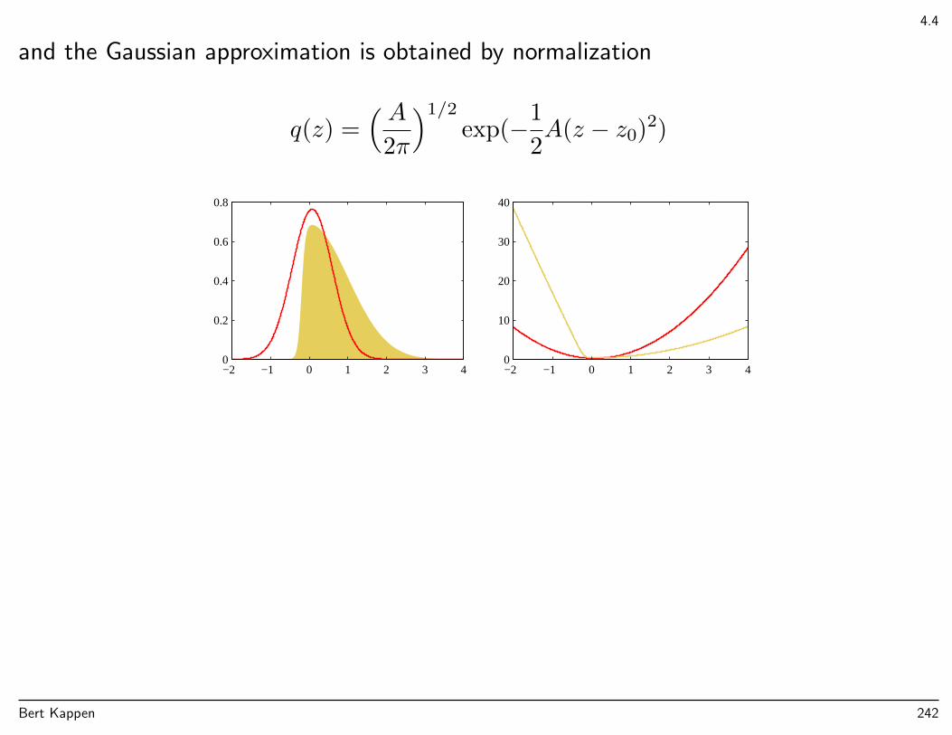
4.4
and the Gaussian approximation is obtained by normalization
q(z) =( A
2π
)1/2
exp(−1
2A(z − z0)2)
−2 −1 0 1 2 3 40
0.2
0.4
0.6
0.8
−2 −1 0 1 2 3 40
10
20
30
40
Bert Kappen 242
4.4
Laplace approximation in M dimensions
In M dimensions results are similar,
q(z) =
(det (A)
(2π)M/2
)exp(−1
2(z − z0)TA(z − z0))
where
Aij = − ∂2
∂zi∂zjln f(z)
∣∣z=z0
Usually z0 is found by numerical optimization.
A weakness of Laplace approximation is that it relies only on the local properties of themode. Other methods (e.g. sampling or variational methods) are based on more globalproperties of p.
Bert Kappen 243
4.4.1
Model comparison and BIC
Approximation of Z:
Z =
∫f(z)dz (4)
≈ f(z0)
∫exp(−1
2(z − z0)TA(z − z0))dz (5)
= f(z0)(2π)M/2
det(A)1/2(6)
Bert Kappen 244
4.4.1
Model comparison and BIC
Application: approximation of model evidence.
f(θ) = p(D|θ)p(θ) (7)
Z = P (D) =
∫p(D|θ)p(θ)dθ (8)
Then applying Laplace approximation, we obtain (Ex. 4. 22)
lnP (D) ≈ ln p(D|θMAP) + ln p(θMAP) +M
2ln 2π − 1
2ln det(A)︸ ︷︷ ︸
Occam factor
whereA = −∇∇ ln p(D|θ)p(θ)
∣∣∣θMAP
= −∇∇p(θ|D)∣∣∣θMAP
which can be interpreted as the inverse width of the posterior.
Bert Kappen 245
4.4.1
Model comparison and BIC
Under some assumptions, A =∑nAn ≈ NA, and full rank, then
ln det(A) ≈ ln det(NA) = ln(NM det(A)) ≈M lnN
leads to the Bayesian Information Criterion (BIC)
lnP (D) ≈ ln p(D|θMAP)− 1
2M lnN (+const.)
Bert Kappen 246
4.5
Bayesian logistic regression
Prior p(w) = N (w|m0,S0)
Log posterior = log prior + log likelihood + const
ln p(w|t) = −1
2(w −m0)TS−1
0 (w −m0)
+∑n
tn ln yn + (1− tn) ln(1− yn)+ const
where yn = σ(wTφn).
Posterior distribution in p(w|t)?
Laplace approximation: find wMAP and compute second derivatives:
S−1N = −∇∇ ln p(w|t) = S−1
0 +∑n
yn(1− yn)φnφTn
andq(w) = N (w|wMAP,SN)
Bert Kappen 247
4.5
Predictive distribution
p(C1|φ, t) =
∫σ(wTφ)p(w|t)dw ≈
∫σ(wTφ)q(w)dw
The function σ(wTφ) depends only on w via its projection on φ. We can marginalizeout the other variables, since q is a Gaussian. The marginal is then again a Gaussian forwhich we can compute its parameters∫
σ(wTφ)q(w)dw =
∫σ(a)N (a|µa, σ2
a)da
where the parameters turn out to be µa = wTMAPφ and σ2
a = φTSNφ.
Unfortunately, this integral cannot be expressed analytically. However σ(x) is wellapproximated by the probit function, i.e., the cumulative Gaussian
Φ(x) =
∫ x
∞N (u|0, 1)du
In particular σ(x) ≈ Φ(√
π8x). With additional manipulations the predictive distributions
Bert Kappen 248
4.5
can be shown to be approximated by
p(C1|φ, t) ≈ σ((1 + πσ2a/8)−1/2µa) = σ(κ(σ2
a)µa)
Note that the MAP predictive distribution is
p(C1|φ,wMAP ) = σ(µa).
The decision boundary p(C1|φ, . . .) = 0.5 is the same in both approximations, namely atµa = 0. Since κ < 1, the Laplace approximation is less certain about the classifications.
Bert Kappen 249
An overview of some more powerful models and methods
Non-linear methods using a fixed set of basis functions (polynomials) (chapter 3,4) sufferfrom curse of dimensionality.
A succesful alternative is to adapt the basis functions to the problem.
Bert Kappen 250
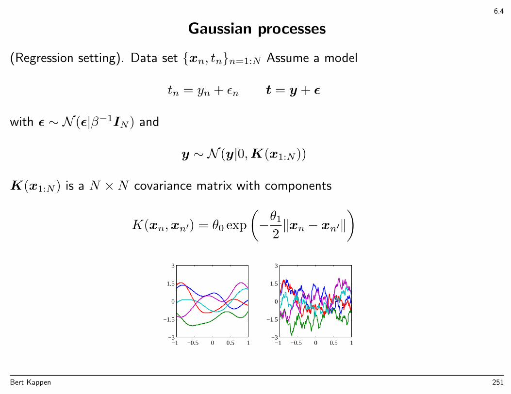
6.4
Gaussian processes
(Regression setting). Data set xn, tnn=1:N Assume a model
tn = yn + εn t = y + ε
with ε ∼ N (ε|β−1IN) and
y ∼ N (y|0,K(x1:N))
K(x1:N) is a N ×N covariance matrix with components
K(xn,xn′) = θ0 exp
(−θ1
2‖xn − xn′‖
)
−1 −0.5 0 0.5 1−3
−1.5
0
1.5
3
−1 −0.5 0 0.5 1−3
−1.5
0
1.5
3
Bert Kappen 251
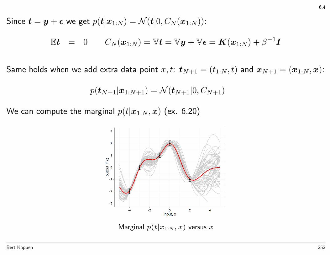
6.4
Since t = y + ε we get p(t|x1:N) = N (t|0, CN(x1:N)):
Et = 0 CN(x1:N) = Vt = Vy + Vε = K(x1:N) + β−1I
Same holds when we add extra data point x, t: tN+1 = (t1:N , t) and xN+1 = (x1:N ,x):
p(tN+1|x1:N+1) = N (tN+1|0, CN+1)
We can compute the marginal p(t|x1:N ,x) (ex. 6.20)
Marginal p(t|x1:N , x) versus x
Bert Kappen 252
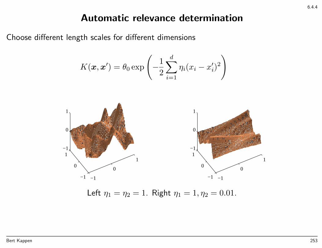
6.4.4
Automatic relevance determination
Choose different length scales for different dimensions
K(x,x′) = θ0 exp
(−1
2
d∑i=1
ηi(xi − x′i)2
)
−1
0
1
−1
0
1−1
0
1
−1
0
1
−1
0
1−1
0
1
Left η1 = η2 = 1. Right η1 = 1, η2 = 0.01.
Bert Kappen 253
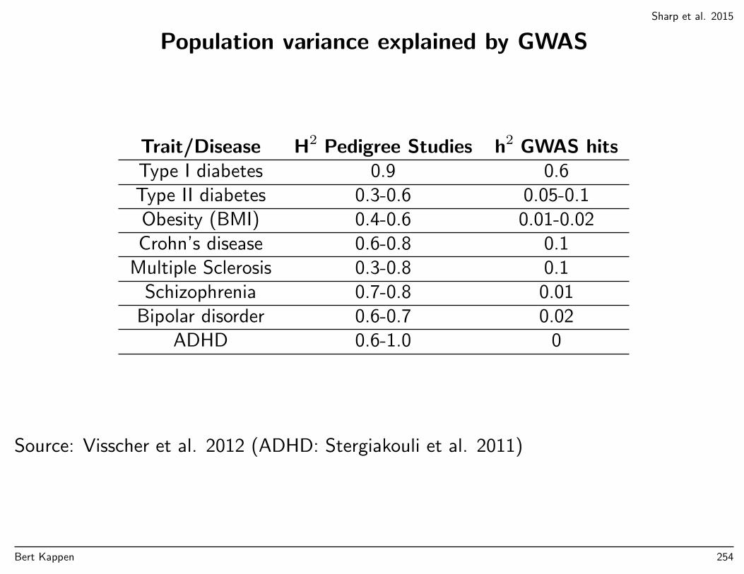
Sharp et al. 2015
Population variance explained by GWAS
Trait/Disease H2 Pedigree Studies h2 GWAS hitsType I diabetes 0.9 0.6Type II diabetes 0.3-0.6 0.05-0.1Obesity (BMI) 0.4-0.6 0.01-0.02Crohn’s disease 0.6-0.8 0.1
Multiple Sclerosis 0.3-0.8 0.1Schizophrenia 0.7-0.8 0.01
Bipolar disorder 0.6-0.7 0.02ADHD 0.6-1.0 0
Source: Visscher et al. 2012 (ADHD: Stergiakouli et al. 2011)
Bert Kappen 254

Sharp et al. 2015
Features of the regression problem
• Sparse
– More dimensions than data samples– Low number of significant SNPs
• Unknown mechanism
– Possible interaction models are of unknown order and complexity.
• Common approaches
– linear univariate or pairwise– path ways
Bert Kappen 255
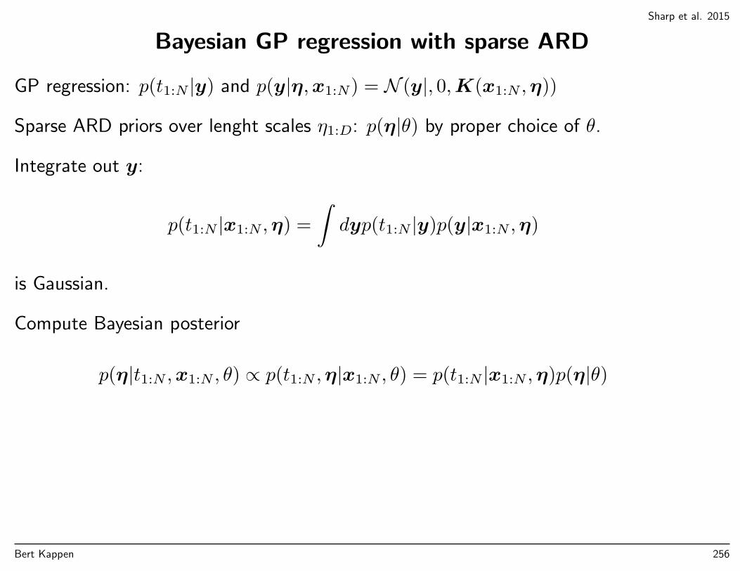
Sharp et al. 2015
Bayesian GP regression with sparse ARD
GP regression: p(t1:N |y) and p(y|η,x1:N) = N (y|, 0,K(x1:N ,η))
Sparse ARD priors over lenght scales η1:D: p(η|θ) by proper choice of θ.
Integrate out y:
p(t1:N |x1:N ,η) =
∫dyp(t1:N |y)p(y|x1:N ,η)
is Gaussian.
Compute Bayesian posterior
p(η|t1:N ,x1:N , θ) ∝ p(t1:N ,η|x1:N , θ) = p(t1:N |x1:N ,η)p(η|θ)
Bert Kappen 256
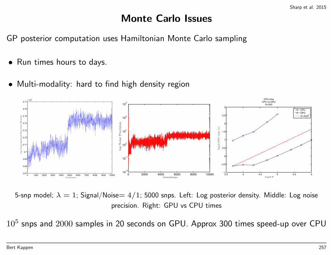
Sharp et al. 2015
Monte Carlo Issues
GP posterior computation uses Hamiltonian Monte Carlo sampling
• Run times hours to days.
• Multi-modality: hard to find high density region
0 1000 2000 3000 4000 5000 6000 7000 8000 9000 100002.67
2.68
2.69
2.7
2.71
2.72
2.73
2.74
2.75
2.76
2.77x 10
4
i te ration s
logUnnormalised
PosteriorDensity
0 2000 4000 6000 8000 1000010
−2
10−1
100
101
102
103
i terations
logNoisePrecision
3.5 4 4.5 5 5.5 6−1
−0.5
0
0.5
1
1.5
2
2.5
3
l og10 P
log10CPU
time(s)
CPU timeCPU vs GPU
N=500
CPU
GPU
(P+N)N2
5-snp model; λ = 1; Signal/Noise= 4/1; 5000 snps. Left: Log posterior density. Middle: Log noise
precision. Right: GPU vs CPU times
105 snps and 2000 samples in 20 seconds on GPU. Approx 300 times speed-up over CPU
Bert Kappen 257
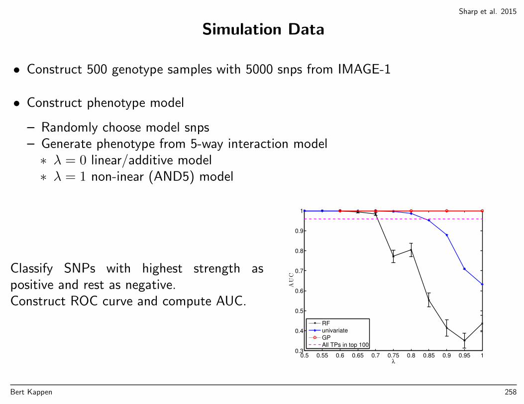
Sharp et al. 2015
Simulation Data
• Construct 500 genotype samples with 5000 snps from IMAGE-1
• Construct phenotype model
– Randomly choose model snps– Generate phenotype from 5-way interaction model∗ λ = 0 linear/additive model∗ λ = 1 non-inear (AND5) model
Classify SNPs with highest strength aspositive and rest as negative.Construct ROC curve and compute AUC.
0.5 0.55 0.6 0.65 0.7 0.75 0.8 0.85 0.9 0.95 10.3
0.4
0.5
0.6
0.7
0.8
0.9
1
λ
AUC
RF
univariate
GP
All TPs in top 100
Bert Kappen 258
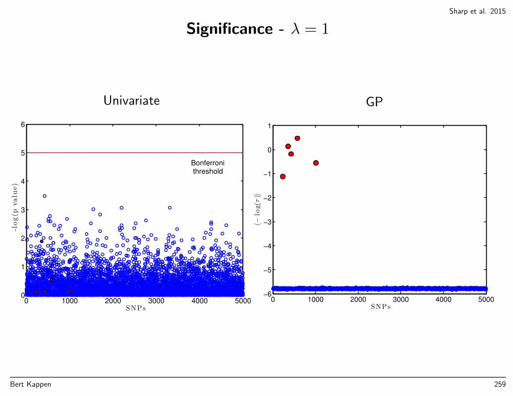
Sharp et al. 2015
Significance - λ = 1
Univariate
0 1000 2000 3000 4000 50000
1
2
3
4
5
6
Bonferroni
threshold
SNPs
-log(p
valu
e)
GP
0 1000 2000 3000 4000 5000−6
−5
−4
−3
−2
−1
0
1
SNPs
〈−log(τ)〉
Bert Kappen 259

Sharp et al. 2015
Finding missing heritability in Yeast (Bloom et al., Nat. 2013.)
• 1008 genetically distinct inbred cell-lines. 46 different phenotypes.
• Pairwise interactions explain additional 3 % median genetic variance per trait.
0 0.1 0.2 0.3 0.4 0.5 0.6 0.7 0.8 0.9 10
0.1
0.2
0.3
0.4
0.5
0.6
0.7
0.8
0.9
1
H2 (Anova estimate)
H2(GPestim
ate)
Bert Kappen 260
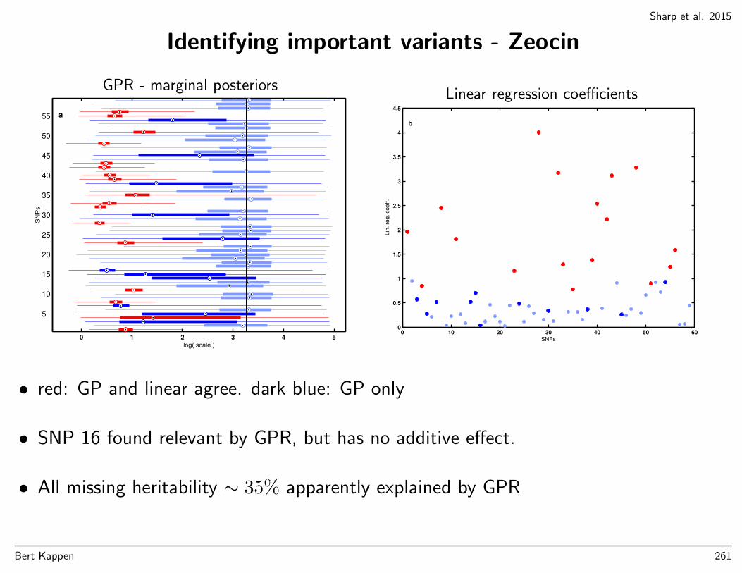
Sharp et al. 2015
Identifying important variants - Zeocin
GPR - marginal posteriors
0 1 2 3 4 5
5
10
15
20
25
30
35
40
45
50
55
SN
Ps
log( scale )
a
Linear regression coefficients
0 10 20 30 40 50 600
0.5
1
1.5
2
2.5
3
3.5
4
4.5
SNPs
Lin
. re
g.
co
eff
.
b
• red: GP and linear agree. dark blue: GP only
• SNP 16 found relevant by GPR, but has no additive effect.
• All missing heritability ∼ 35% apparently explained by GPR
Bert Kappen 261
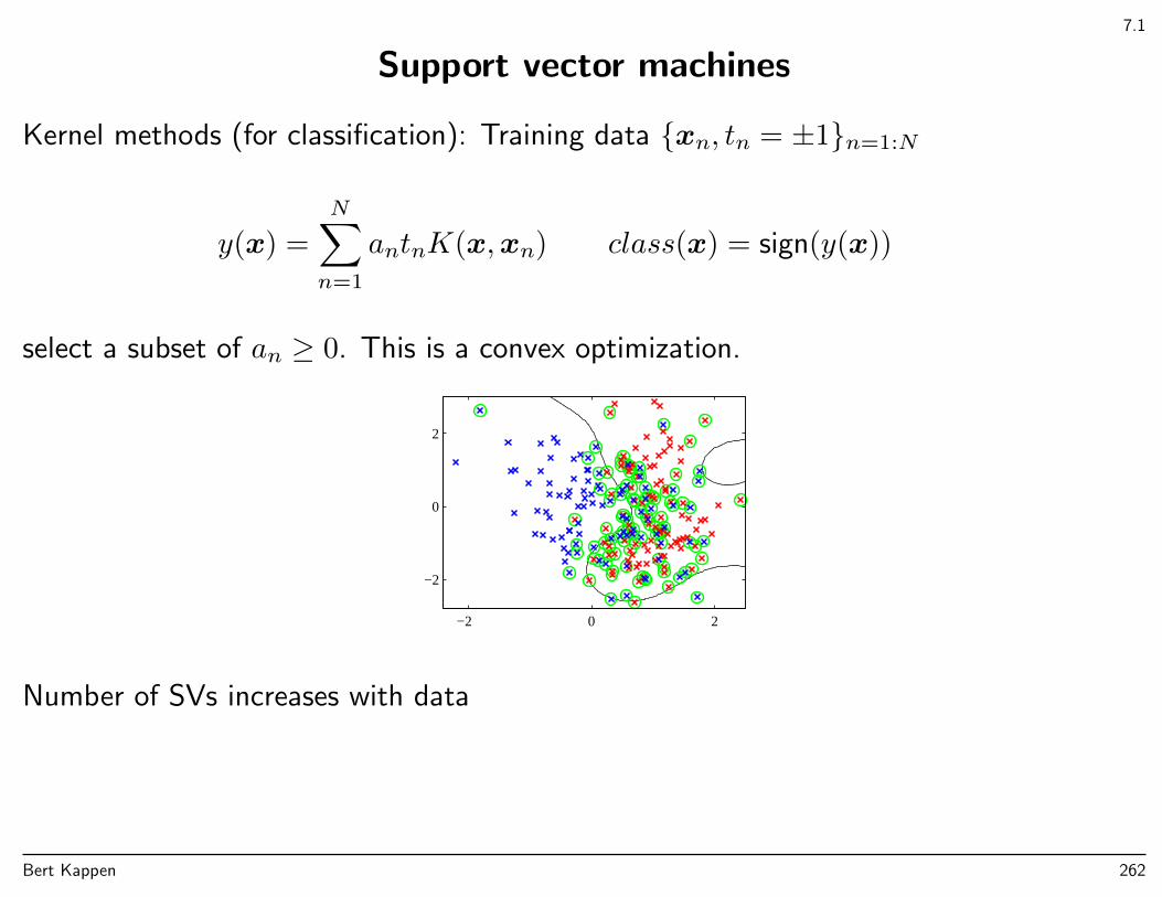
7.1
Support vector machines
Kernel methods (for classification): Training data xn, tn = ±1n=1:N
y(x) =
N∑n=1
antnK(x,xn) class(x) = sign(y(x))
select a subset of an ≥ 0. This is a convex optimization.
−2 0 2
−2
0
2
Number of SVs increases with data
Bert Kappen 262
5.1
Feed-forward Network functions
We extend the previous regression model with fixed basis functions
y(x,w) = f
M∑j=1
wjφj(x)
to a model where φj is adaptive:
φj(x) = h(
D∑i=0
w(1)ji xi)
Bert Kappen 263
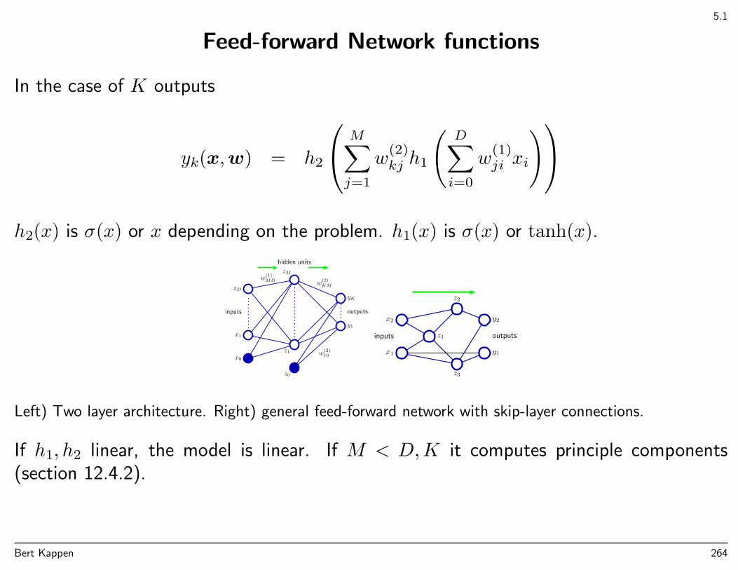
5.1
Feed-forward Network functions
In the case of K outputs
yk(x,w) = h2
M∑j=1
w(2)kj h1
(D∑i=0
w(1)ji xi
)h2(x) is σ(x) or x depending on the problem. h1(x) is σ(x) or tanh(x).
x0
x1
xD
z0
z1
zM
y1
yK
w(1)MD w
(2)KM
w(2)10
hidden units
inputs outputs
x1
x2
z1
z3
z2
y1
y2
inputs outputs
Left) Two layer architecture. Right) general feed-forward network with skip-layer connections.
If h1, h2 linear, the model is linear. If M < D,K it computes principle components(section 12.4.2).
Bert Kappen 264
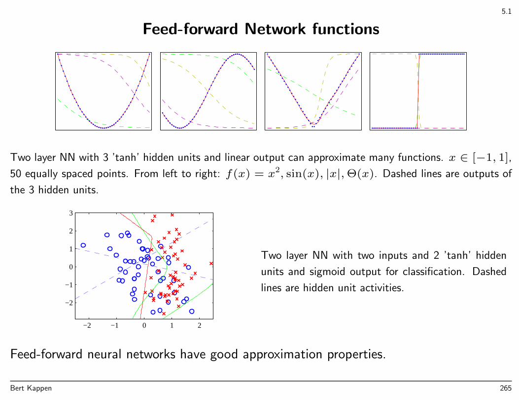
5.1
Feed-forward Network functions
Two layer NN with 3 ’tanh’ hidden units and linear output can approximate many functions. x ∈ [−1, 1],
50 equally spaced points. From left to right: f(x) = x2, sin(x), |x|,Θ(x). Dashed lines are outputs of
the 3 hidden units.
−2 −1 0 1 2
−2
−1
0
1
2
3
Two layer NN with two inputs and 2 ’tanh’ hidden
units and sigmoid output for classification. Dashed
lines are hidden unit activities.
Feed-forward neural networks have good approximation properties.
Bert Kappen 265

5.1.1
Weight space symmetries
For any solutions of the weights, there are many equivalent solutions due to symmetry:- for any hidden unit j with tanh activation function, change wji → −wji and wkj →−wkj: 2M solutions- rename the hidden unit labels: M ! solutions
Thus a total of M !2M equivalent solutions, not only for tanh activation functions.
Bert Kappen 266
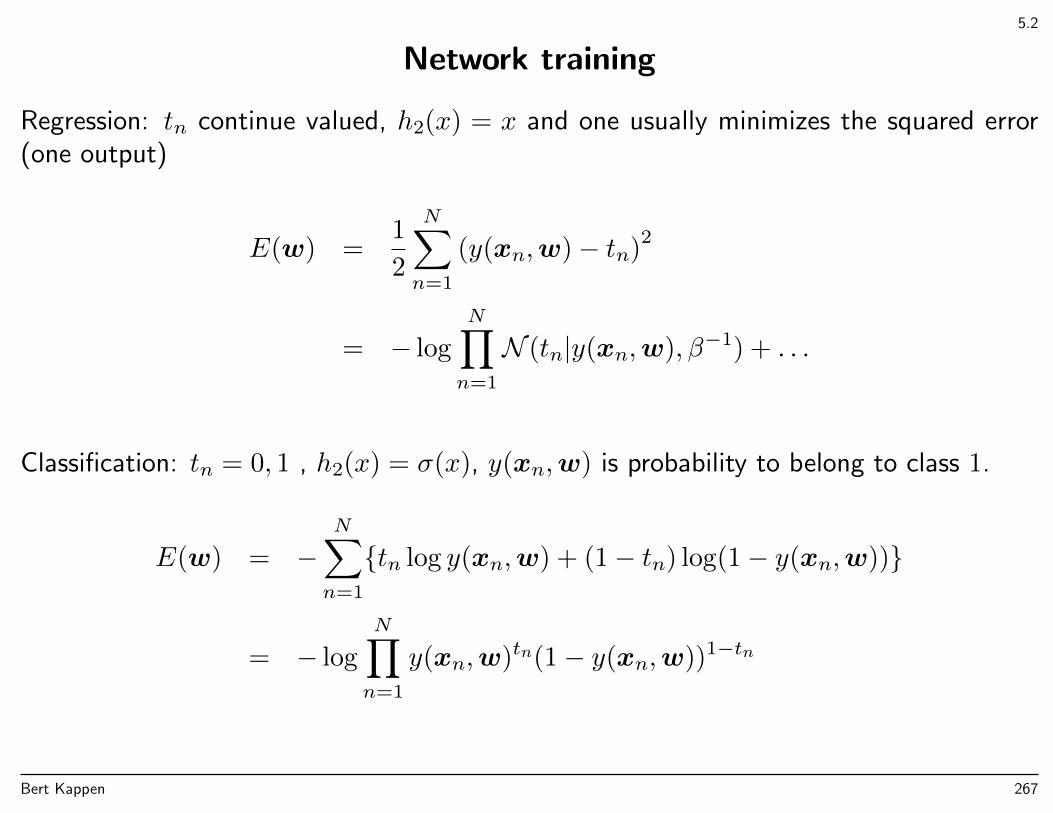
5.2
Network training
Regression: tn continue valued, h2(x) = x and one usually minimizes the squared error(one output)
E(w) =1
2
N∑n=1
(y(xn,w)− tn)2
= − log
N∏n=1
N (tn|y(xn,w), β−1) + . . .
Classification: tn = 0, 1 , h2(x) = σ(x), y(xn,w) is probability to belong to class 1.
E(w) = −N∑n=1
tn log y(xn,w) + (1− tn) log(1− y(xn,w))
= − log
N∏n=1
y(xn,w)tn(1− y(xn,w))1−tn
Bert Kappen 267
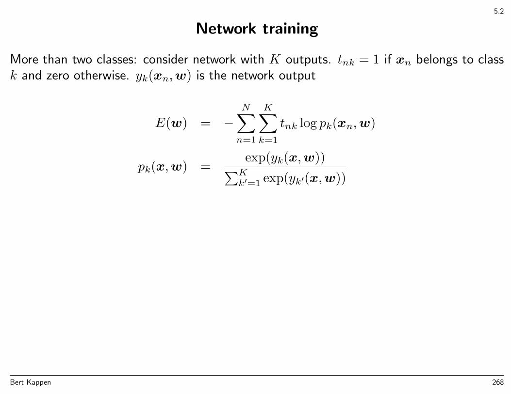
5.2
Network training
More than two classes: consider network with K outputs. tnk = 1 if xn belongs to classk and zero otherwise. yk(xn,w) is the network output
E(w) = −N∑n=1
K∑k=1
tnk log pk(xn,w)
pk(x,w) =exp(yk(x,w))∑Kk′=1 exp(yk′(x,w))
Bert Kappen 268
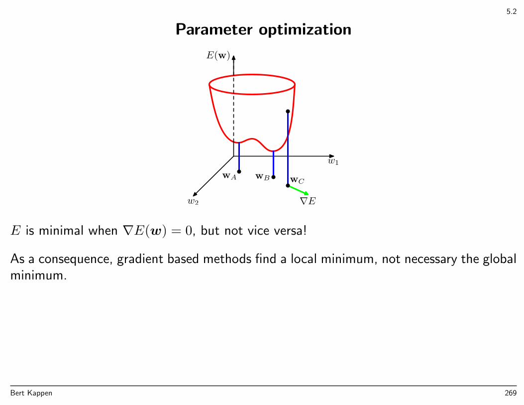
5.2
Parameter optimization
w1
w2
E(w)
wA wB wC
∇E
E is minimal when ∇E(w) = 0, but not vice versa!
As a consequence, gradient based methods find a local minimum, not necessary the globalminimum.
Bert Kappen 269
5.2
Gradient descent optimization
The simplest procedure to optimize E is to start with a random w and iterate
wτ+1 = wτ − η∇E(wτ)
This is called batch learning, where all training data are included in the computation of∇E.
One can also consider on-line learing, where only one or a subset of training patterns isconsidered for computing ∇E.
E(w) =∑n
En(w) wτ+1 = wτ − η∇En(wτ)
May be efficient for large data sets. This results in a stochastic dynamics in w that canhelp to escape local minima.
Bert Kappen 270
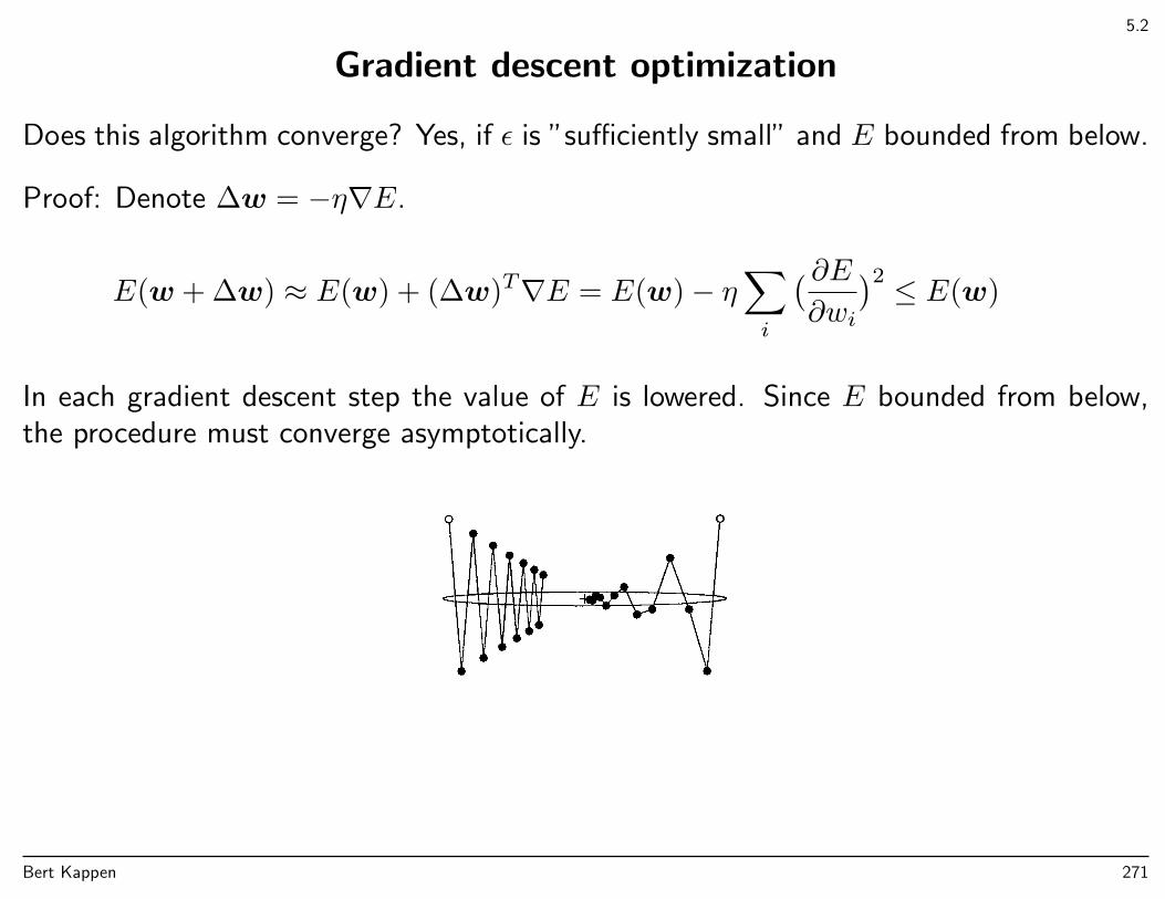
5.2
Gradient descent optimization
Does this algorithm converge? Yes, if ε is ”sufficiently small” and E bounded from below.
Proof: Denote ∆w = −η∇E.
E(w + ∆w) ≈ E(w) + (∆w)T∇E = E(w)− η∑i
( ∂E∂wi
)2 ≤ E(w)
In each gradient descent step the value of E is lowered. Since E bounded from below,the procedure must converge asymptotically.
Bert Kappen 271
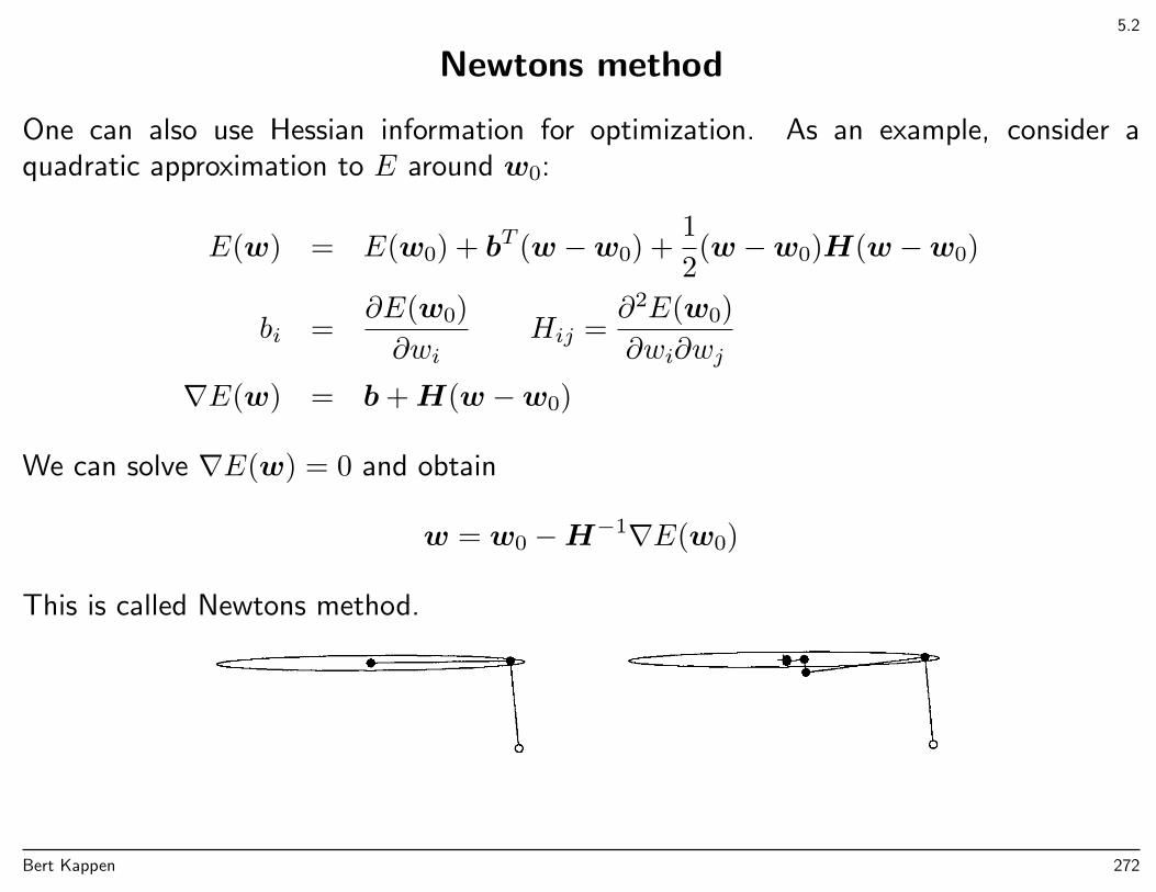
5.2
Newtons method
One can also use Hessian information for optimization. As an example, consider aquadratic approximation to E around w0:
E(w) = E(w0) + bT (w −w0) +1
2(w −w0)H(w −w0)
bi =∂E(w0)
∂wiHij =
∂2E(w0)
∂wi∂wj
∇E(w) = b+H(w −w0)
We can solve ∇E(w) = 0 and obtain
w = w0 −H−1∇E(w0)
This is called Newtons method.
Bert Kappen 272
5.3.1
Error backpropagation
Error is sum of error per pattern
E(w) =∑n
En(w) En(w) =1
2‖y(xn,w)− tn‖2
yk(x,w) = h2
wk0 +
M∑j=1
wkjh1
(wj0 +
D∑i=1
wjixi
)= h2(ak)
ak = wk0 +
M∑j=1
wkjh1(aj) =
M∑j=0
wkjh1(aj) h1(a0) = 1
aj = wj0 +
D∑i=1
wjixi =
D∑i=0
wjixi x0 = 1
Bert Kappen 273
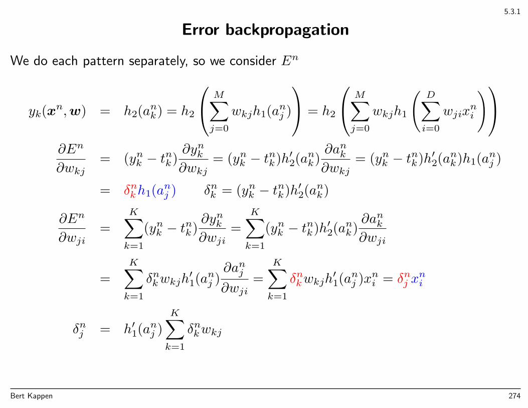
5.3.1
Error backpropagation
We do each pattern separately, so we consider En
yk(xn,w) = h2(ank) = h2
M∑j=0
wkjh1(anj )
= h2
M∑j=0
wkjh1
(D∑i=0
wjixni
)∂En
∂wkj= (ynk − tnk)
∂ynk∂wkj
= (ynk − tnk)h′2(ank)∂ank∂wkj
= (ynk − tnk)h′2(ank)h1(anj )
= δnkh1(anj ) δnk = (ynk − tnk)h′2(ank)
∂En
∂wji=
K∑k=1
(ynk − tnk)∂ynk∂wji
=
K∑k=1
(ynk − tnk)h′2(ank)∂ank∂wji
=
K∑k=1
δnkwkjh′1(anj )
∂anj∂wji
=
K∑k=1
δnkwkjh′1(anj )xni = δnj x
ni
δnj = h′1(anj )
K∑k=1
δnkwkj
Bert Kappen 274
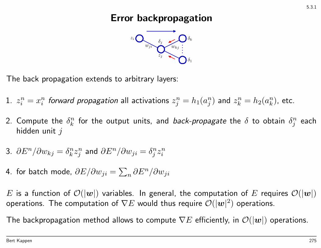
5.3.1
Error backpropagation
zi
zj
δjδk
δ1
wji wkj
The back propagation extends to arbitrary layers:
1. zni = xni forward propagation all activations znj = h1(anj ) and znk = h2(ank), etc.
2. Compute the δnk for the output units, and back-propagate the δ to obtain δnj eachhidden unit j
3. ∂En/∂wkj = δnkznj and ∂En/∂wji = δnj z
ni
4. for batch mode, ∂E/∂wji =∑n ∂E
n/∂wji
E is a function of O(|w|) variables. In general, the computation of E requires O(|w|)operations. The computation of ∇E would thus require O(|w|2) operations.
The backpropagation method allows to compute ∇E efficiently, in O(|w|) operations.
Bert Kappen 275
5.4
Newtons method
Note that this is expensive since H is large and needs to be inverted. A simpleapproximation is to only consider the diagonal elements of the Hessian (section 5.4.1),the Levenberg-Marquardt approximation (section 5.4.2) or approximate inverse Hessiansconjugate gradient methods (section 5.4.3).
Bert Kappen 276
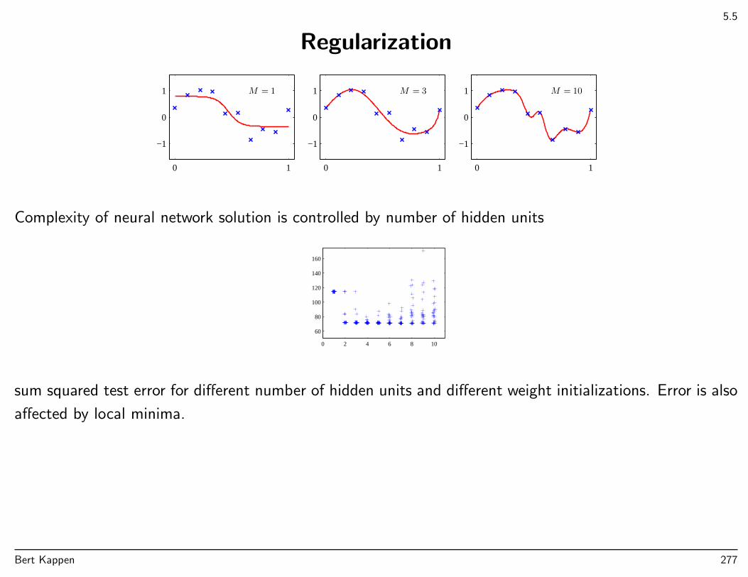
5.5
Regularization
M = 1
0 1
−1
0
1 M = 3
0 1
−1
0
1 M = 10
0 1
−1
0
1
Complexity of neural network solution is controlled by number of hidden units
0 2 4 6 8 10
60
80
100
120
140
160
sum squared test error for different number of hidden units and different weight initializations. Error is also
affected by local minima.
Bert Kappen 277
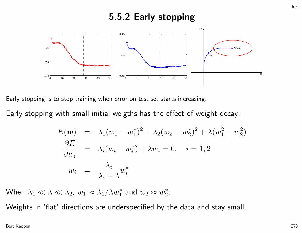
5.5
5.5.2 Early stopping
0 10 20 30 40 500.15
0.2
0.25
0 10 20 30 40 500.35
0.4
0.45
w1
w2
w
wML
Early stopping is to stop training when error on test set starts increasing.
Early stopping with small initial weigths has the effect of weight decay:
E(w) = λ1(w1 − w∗1)2 + λ2(w2 − w∗2)2 + λ(w21 − w2
2)
∂E
∂wi= λi(wi − w∗i ) + λwi = 0, i = 1, 2
wi =λi
λi + λw∗i
When λ1 λ λ2, w1 ≈ λ1/λw∗1 and w2 ≈ w∗2.
Weights in ’flat’ directions are underspecified by the data and stay small.
Bert Kappen 278
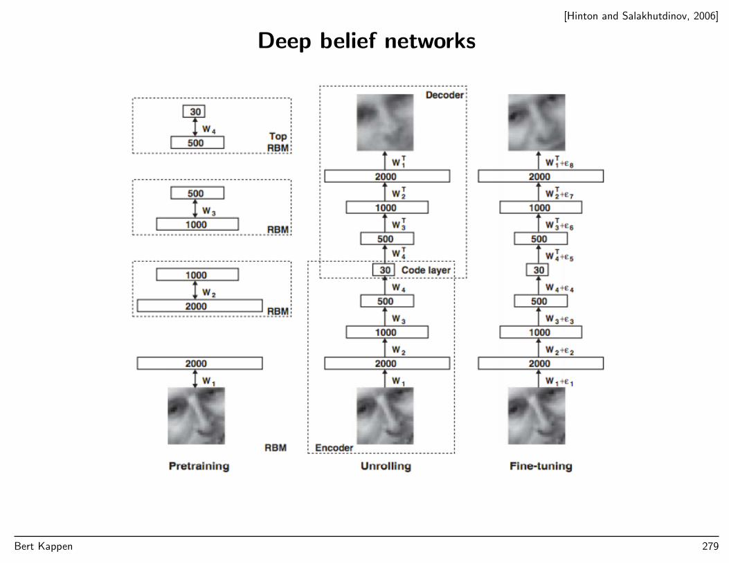
[Hinton and Salakhutdinov, 2006]
Deep belief networks
Bert Kappen 279
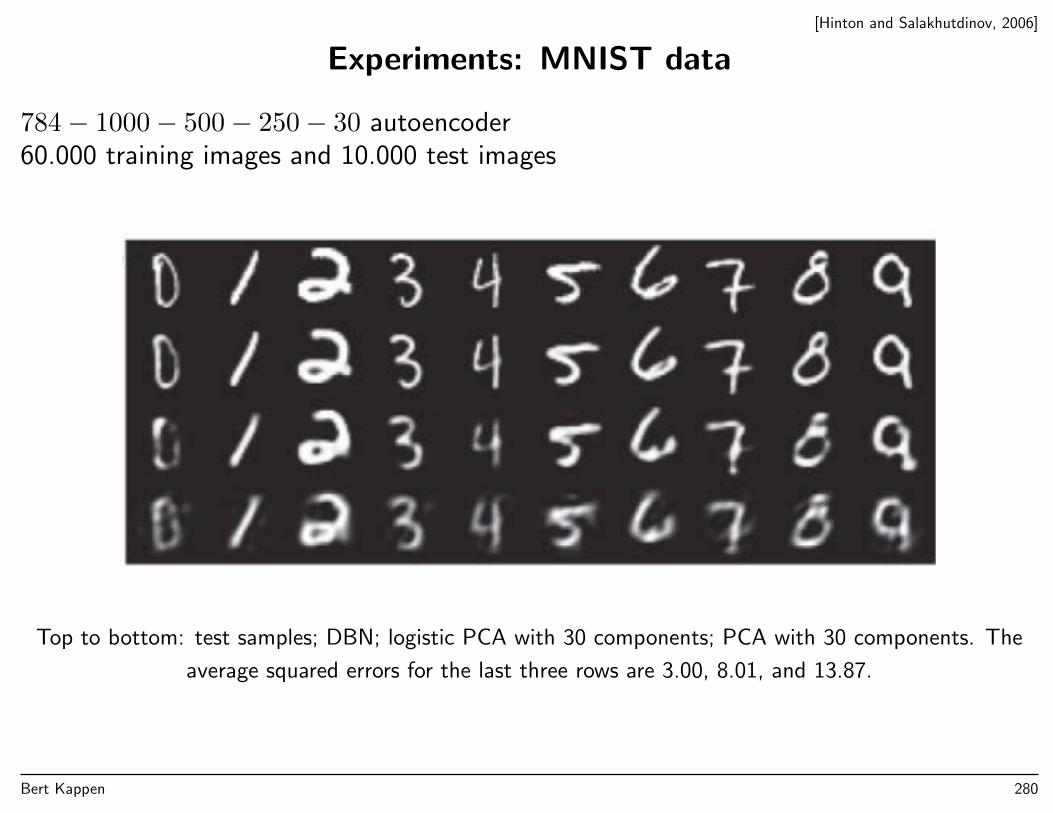
[Hinton and Salakhutdinov, 2006]
Experiments: MNIST data
784− 1000− 500− 250− 30 autoencoder60.000 training images and 10.000 test images
Top to bottom: test samples; DBN; logistic PCA with 30 components; PCA with 30 components. The
average squared errors for the last three rows are 3.00, 8.01, and 13.87.
Bert Kappen 280
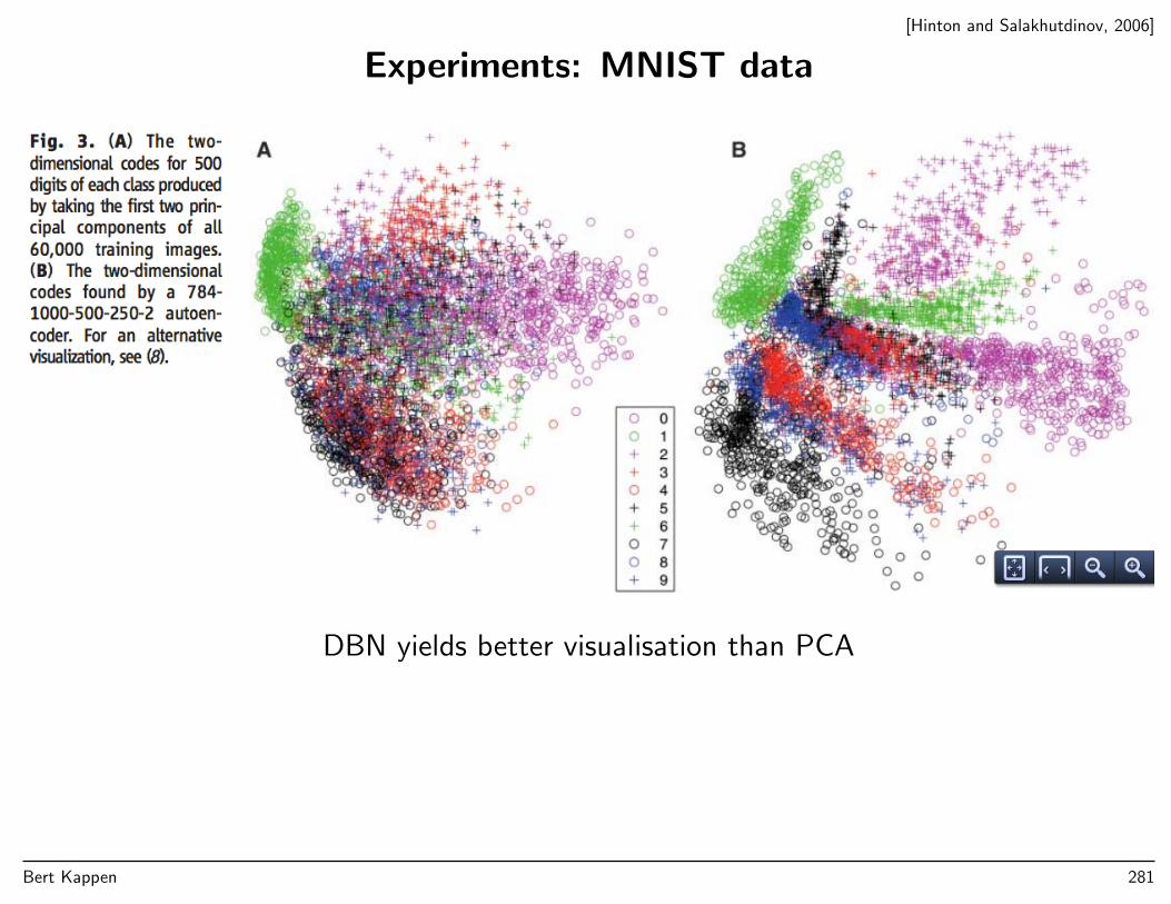
[Hinton and Salakhutdinov, 2006]
Experiments: MNIST data
DBN yields better visualisation than PCA
Bert Kappen 281
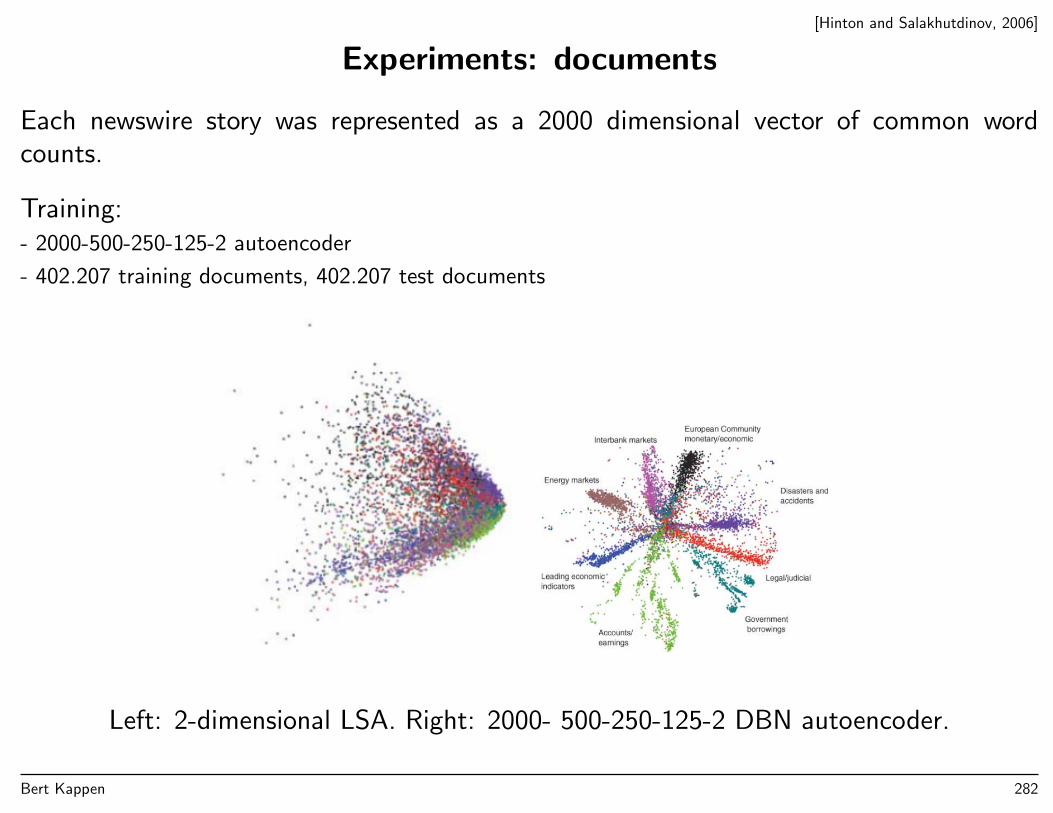
[Hinton and Salakhutdinov, 2006]
Experiments: documents
Each newswire story was represented as a 2000 dimensional vector of common wordcounts.
Training:- 2000-500-250-125-2 autoencoder
- 402.207 training documents, 402.207 test documents
Left: 2-dimensional LSA. Right: 2000- 500-250-125-2 DBN autoencoder.
Bert Kappen 282
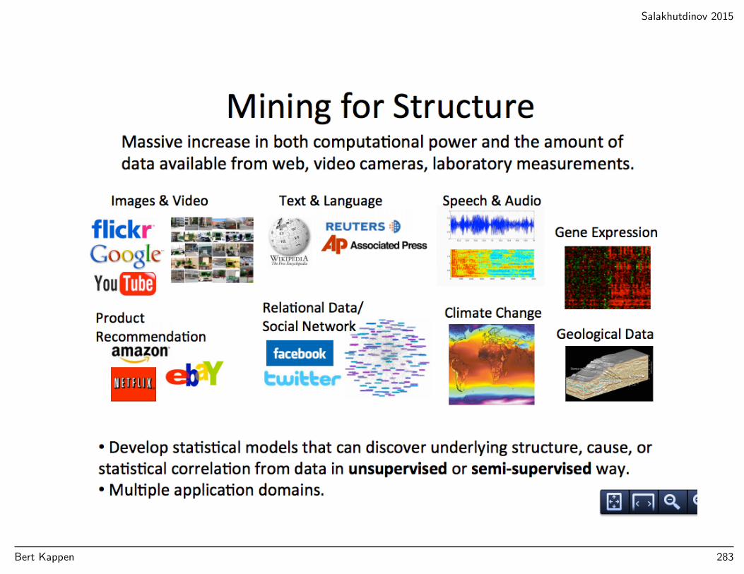
Salakhutdinov 2015
Bert Kappen 283
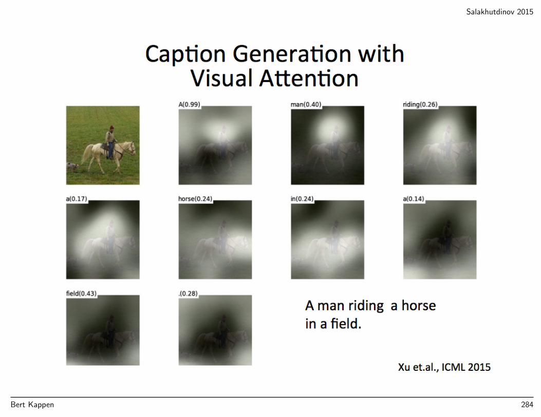
Salakhutdinov 2015
Bert Kappen 284

Salakhutdinov 2015
Bert Kappen 285
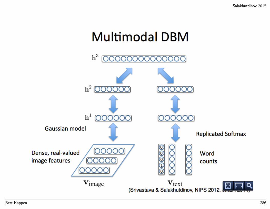
Salakhutdinov 2015
Bert Kappen 286

Salakhutdinov 2015
Bert Kappen 287

Salakhutdinov 2015
Bert Kappen 288

[Mnih et al., 2015]
Human-level control through deep reinforcement learning
http://www.nature.com/nature/journal/v518/n7540/full/nature14236.html#videos
Bert Kappen 289
[Mnih et al., 2015]
References
References
[Hinton and Salakhutdinov, 2006] Hinton, G. E. and Salakhutdinov, R. R. (2006). Reducing the
dimensionality of data with neural networks. Science, 313(5786):504–507.
[Mnih et al., 2015] Mnih, V., Kavukcuoglu, K., Silver, D., Rusu, A. A., Veness, J., Bellemare, M. G.,
Graves, A., Riedmiller, M., Fidjeland, A. K., Ostrovski, G., et al. (2015). Human-level control through
deep reinforcement learning. Nature, 518(7540):529–533.
Bert Kappen 290