Introduction to LATEX

John Richard Pawlina

UConn Math Major Alumnus

Compiled on August 26, 2018

Abstract

This document aims to familiarize the reader with skills in LATEX for undergraduate writing.

We begin with a general introduction to the program, with a rundown of what one can find in

most LATEX distribution packages. The first main section explains how to use LATEX as a word

processor, and from there we move on to basic and advanced types of math typesetting.

It should be noted that this article was written with the TEXworks LATEX editor, and assumes

the reader is following along with the same editor. What one finds in one editor is usually exactly

what he would find in another editor, but the layouts can vary. So long as the reader is aware

of that, he will not have issue following along while using an editor other than TEXworks.

Contents

1 Introduction 3

2 LATEX as a Word Processor 5

2.1 Overview of a TeX Document . . . . . . . . . . . . . . . . . . . . . . . . . . . . . . . 5

2.2 Typical Formatting Options . . . . . . . . . . . . . . . . . . . . . . . . . . . . . . . . 6

2.3 Creating a Title Page . . . . . . . . . . . . . . . . . . . . . . . . . . . . . . . . . . . 7

2.4 Sectioning and Organization . . . . . . . . . . . . . . . . . . . . . . . . . . . . . . . . 8

2.5 Paragraphing . . . . . . . . . . . . . . . . . . . . . . . . . . . . . . . . . . . . . . . . 10

2.6 Usual Word Processing Functions . . . . . . . . . . . . . . . . . . . . . . . . . . . . . 11

3 Lists, Tables, and Bibliographies 13

3.1 The Itemize and Enumerate Environments . . . . . . . . . . . . . . . . . . . . . . . . 13

3.2 Tabular Environments . . . . . . . . . . . . . . . . . . . . . . . . . . . . . . . . . . . 14

3.3 Bibliographies . . . . . . . . . . . . . . . . . . . . . . . . . . . . . . . . . . . . . . . . 16

3.4 Presenting Verbatim Code . . . . . . . . . . . . . . . . . . . . . . . . . . . . . . . . . 17

4 Basic Math Typesetting 19

4.1 Relevant Packages . . . . . . . . . . . . . . . . . . . . . . . . . . . . . . . . . . . . . 19

4.2 Basics of Math Mode . . . . . . . . . . . . . . . . . . . . . . . . . . . . . . . . . . . . 19

4.3 Relevant Environments . . . . . . . . . . . . . . . . . . . . . . . . . . . . . . . . . . . 21

4.4 Typical Functions in Math Mode . . . . . . . . . . . . . . . . . . . . . . . . . . . . . 24

5 Advanced Typesetting in Math Mode 26

5.1 Types of Math Fonts . . . . . . . . . . . . . . . . . . . . . . . . . . . . . . . . . . . . 26

5.2 Matrices . . . . . . . . . . . . . . . . . . . . . . . . . . . . . . . . . . . . . . . . . . . 27

5.3 Piecewise Functions . . . . . . . . . . . . . . . . . . . . . . . . . . . . . . . . . . . . 29

5.4 Typical Mathematical Shorthand and Special Symbols . . . . . . . . . . . . . . . . . 30

5.5 Special Arrows and Over- or Under-braces . . . . . . . . . . . . . . . . . . . . . . . . 31

5.6 The stackrel Command . . . . . . . . . . . . . . . . . . . . . . . . . . . . . . . . . . 32

6 Final Words 33

6.1 Recommended Resources . . . . . . . . . . . . . . . . . . . . . . . . . . . . . . . . . 33

6.2 Troubleshooting Tips . . . . . . . . . . . . . . . . . . . . . . . . . . . . . . . . . . . . 33

2

1 Introduction

LATEX, pronounced “lah-tech” or occasionally “lay-tech,” is a program used often when writing math-

ematics. The program is, with a bit of practice, convenient for quickly typesetting proofs, problems

(e.g. for a quiz), and entire articles that are filled with mathematical symbols and shorthand. It

is also great for organizing one’s work and quickly editing errors. (Correcting an error in a hand-

written document can be painstakingly annoying, but editing a line or two of code can be much

simpler.) LATEX does come with some disadvantages, but they mostly reside in the area of coding.

For example, those who have done some sort of coding before may find that learning to use LATEX is

very intuitive, but even the best of us can have difficulty troubleshooting compiling or typesetting

errors when we do not have a fair amount of experience.

In the above paragraph I mentioned typesetting. When we use a LATEX editor, we are writing

code that the editor then compiles into our document. To typeset with TEXworks, you can select the

first option under the Typeset tab, press the green button on the top of the editor, or press Ctrl+t.

When you have written something in LATEX you will not be done with your document until you

have compiled it, and you may have to compile the document a few times to work out some errors

(such as errors in counts, which we discuss in 2.4, that the document uses). By default TEXworks

compiles your code into a Portable Document Format file, or PDF, but this is not the only format

you can use. Under the Typset tab at the top of the editor you may select several other file types

to create. Usually we will create PDFs, so for the remainder of the article we will give instructions

pertaining to that format. Other formats may have different nuances than PDFs, so if you wish to

create something other than a PDF you should do more research to prepare. The final section of

this article gives some resources to investigate.

When you begin your first document in LATEX your writing will look like that of a Word docu-

ment; it will be a lot of black text on a white background. This can be troublesome when coding as

it leaves much for anyone, as the coder or one looking over some code, to interpret on his own. I sug-

gest that you always adjust your settings to be most convenient for you. When opening TEXworks,

I always select three options. First, I look under the Format tab and select Line Numbers. This

helps significantly when later looking for errors because the error will always reference a line number.

It also aids in keeping track of how I have organized my code, so that I can see when I have put

too much in one line (thus making it harder to distinguish where exactly my errors lie). Second,

I choose Format>Syntax Coloring>LaTeX. This option brings color to your code, and will be one

of your best tools while writing code. The LATEX syntax coloring option colors your code based on

what it is. That is, notes in the code (section 2.2) appear in red, commands (section 2.2) appear in

blue, environments (section 3) appear in dark green, and command operators (section 2.2) appear in

dark brown. The third recommended setting is to enable spell check under Edit>Spelling>English.

As with Word this underlines misspelled or unknown words with a squiggly red line. This is very

useful while writing code so long as the coder pays attention to his writing as he is writing it. If

one were to wait until the very end of writing his document to check his spelling, he may have a

hard time going about it while the coloring options are enabled and large blocks of texts are present.

What I do in that situation is disable the coloring options, and sometimes I enlarge the text size

3

under Format>Font. The three suggestions and more preferences can be set to default under Edit

>Preferences.

4

2 LATEX as a Word Processor

This document was written in LATEX, though we have yet to see any mathematics. That is because

LATEX is also great as a word processor, and depending on your document class (section 2.2) your

documents will have that unique “math style” you may have noticed in your exams and handouts.

It is crucial to understand that LATEX is not simply for presenting mathematics. It is for presenting

writing that explains mathematics and other topics. Like any piece of writing you compose you

should aim to clearly present your ideas to the reader, even if you use LATEX to write a short proof

or answers to an assignment. This includes revising and redrafting your documents several times

during the writing process. If you are finding it difficult to present your ideas in an effective manner,

you should not hesitate to visit your university’s writing center or other such similar resource.

Knowledge of mathematics and knowledge of good writing should not be mutually exclusive (and in

an ideal world, they would be mutually inclusive). While improving your writing you might be able

to help another improve his mathematics!

That aside, this section aims to present the very basics of LATEX for our use. One will learn how

a document is structured in LATEX and will be given tips for organizing his documents.

2.1 Overview of a TeX Document

This may seem counterintuitive, but before we learn the skeleton structure of a TeX document, we

will learn how to insert notes into the document. This way we can examine examples of verbatim

(“copied word for word”) code that have notes without being too confused by the new information.

Here is an example of what we would put into our code for a note:

Example 2.1. %This is an example of a note.

Here we see one shortfall of LATEX. While in our code the example is red, here in print it is not.

In general our examples will not be so long that colored code will add much to our understanding,

but it is recommended that you follow along with a TeX editor so that you may see firsthand what

the examples do. After I explain how to start a TeX document (with its skeleton), you will easily

be able to copy (and improve, if so motivated) the provided examples.

Now, more importantly, what is our example 2.1 saying? When we use % in our code, everything

following it (on the same line) is considered a note. This code is not typeset and is left only as a way

for the coder to leave a message behind, for himself or others, explaining the code. This is useful

when planning out a document or explaining to a new user of LATEX how to use a new command.

Usually I like to surround a note with % when it is a self-contained note and to use only one % on

the left of the note when the note references the line it is on.

5

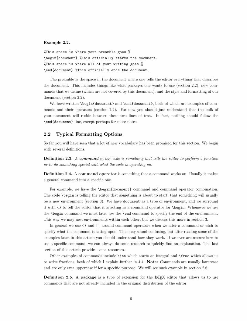
Example 2.2.

%This space is where your preamble goes.%

\begin{document} %This officially starts the document.

%This space is where all of your writing goes.%

\end{document} %This officially ends the document.

The preamble is the space in the document where one tells the editor everything that describes

the document. This includes things like what packages one wants to use (section 2.2), new com-

mands that we define (which are not covered by this document), and the style and formatting of our

document (section 2.2).

We have written \begin{document} and \end{document}, both of which are examples of com-

mands and their operators (section 2.2). For now you should just understand that the bulk of

your document will reside between these two lines of text. In fact, nothing should follow the

\end{document} line, except perhaps for more notes.

2.2 Typical Formatting Options

So far you will have seen that a lot of new vocabulary has been promised for this section. We begin

with several definitions.

Definition 2.3. A command in our code is something that tells the editor to perform a function

or to do something special with what the code is operating on.

Definition 2.4. A command operator is something that a command works on. Usually it makes

a general command into a specific one.

For example, we have the \begin{document} command and command operator combination.

The code \begin is telling the editor that something is about to start, that something will usually

be a new environment (section 3). We have document as a type of environment, and we surround

it with {} to tell the editor that it is acting as a command operator for \begin. Whenever we use

the \begin command we must later use the \end command to specify the end of the environment.

This way we may nest environments within each other, but we discuss this more in section 3.

In general we use {} and [] around command operators when we alter a command or wish to

specify what the command is acting upon. This may sound confusing, but after reading some of the

examples later in this article you should understand how they work. If we ever are unsure how to

use a specific command, we can always do some research to quickly find an explanation. The last

section of this article provides some resources.

Other examples of commands include \int which starts an integral and \frac which allows us

to write fractions, both of which I explain further in 4.4. Note: Commands are usually lowercase

and are only ever uppercase if for a specific purpose. We will see such example in section 2.6.

Definition 2.5. A package is a type of extension for the LATEX editor that allows us to use

commands that are not already included in the original distribution of the editor.

6

In the preamble we also include all packages we will use in the document. One can find what

packages he needs online by referencing the commands he plans to use. All special commands that we

find information on will tell us what package they require unless they are the very basic commands

included in all LATEX editors. Including extraneous packages can slow down the compiling speed of

the editor, so it is not recommended to include in our preamble every package we have ever used.

However, we will often times come back to the same packages and commands in several documents,

so creating a template TeX file from which to begin is not unusual.

To add a package to the preamble, just add \usepackage{[package name]} where we replace

[package name] with the name of the package we wish to include. While writing our preamble it is

important to remain organized, which includes keeping our various packages together. It would not

hurt to arrange the packages by their function or by another enlightening manner so that anyone

who reads the TeX file will have an easy time understanding what we plan to do.

We conclude this section with a discussion of some typical document classes.

Definition 2.6. A document class is a type of document, be it an article, a book, etc.

The document class for this document is the article document class. At the very top of the

preamble we have written \documentclass{article}. The document class should always be the

first thing specified in a document. Two main document classes are the article and amsart (short

for “American Mathematical Society Article”) classes.1 The difference between the two classes is

their “look”. In general the two classes are interchangeable, with their handling of title pages being

the main difference. In article format, the abstract goes after the \maketitle command (section

2.3) if it is used, while in amsart it is written beforehand. Any packages that have “ams” in their

names are automatically included in an amsart document, but not in an article document. In

amsart documents equation numbers (section 4.3) are to the left of equations, but in article

documents the numbers are to the right.

Those are the main differences between the two document classes. Really one can just use

whichever he prefers, as either document class may be manipulated to do as one desires. Let it be

clear then that the remainder of the document assumes the use of the article class.

2.3 Creating a Title Page

A title page is a nice addition to any document we write. It lets the reader know who wrote the

paper and where it came from, as well as when it was produced. This is important in evaluating the

background we might be expected to have to read the paper, as well as for determining if the paper

is still relevant today. A good title page will also include an abstract to explain what is assumed

before the start of the document and what is to be explained by the end of the document.

1The following website was used for information regarding the two classes: http://www.math.uiuc.edu/~hildebr/

tex/tips-packages.html

7

Let us note that I did not use the \maketitle command while writing this document as I am

not a big fan of it.

Example 2.7. This is an example of how one might start a document with the \maketitle com-

mand, as seen on the LATEX wikibook webpage:

\thispagestyle{empty}

\title{The Triangulation of Titling Data in

Non-Linear Gaussian Fashion via $\rho$ Series}

\date{October 31, 475}

\author{John Doe\\ Magic Department, Richard Miles University

\and Richard Row, \LaTeX\ Academy}

\maketitle

Most of the above code seems self-explanatory. The \title, \date, and \author commands do

as one might imagine. The rest is not so obvious.

The command \thispagestyle tells the editor that for the particular page the style empty

should be used. The empty page style has no headings or footers (including page numbers). If

we used \pagestyle we would be declaring the page style for the entire document following the

command. There are other page styles, all of which can be easily found by performing a web search

for “LaTeX page style.” The code $\rho$ is an example of something from math mode and will

be discussed in section 4.2. The code \\ is a line break, used for starting a new line (like pressing

“enter” while using Word) or creating a blank line. The \and command helps separate the names

in the title. The \LaTeX\ command is responsible for creating the special character “LATEX” seen

throughout this document. Finally, the \maketitle command indicates that the TeX preceding it is

to be used for a title page. Should the TeX above it not be on a new page, it will, for most document

classes, automatically be put on one. If we are using the article document class, the title will be

placed at the top of the first page of the document.

We can easily make an abstract with the abstract environment:

Example 2.8.

\begin{abstract}

%Your abstract goes in this space.%

\end{abstract}

As stated before it is important to explain what one requires as prior knowledge and to summarize

what the document covers. Many authors choose to include, after their abstracts, references for their

documents and for prior reading.

2.4 Sectioning and Organization

Organization is key to presenting any information to your reader. This document would not be

very helpful if it were not broken into sections. Primarily we are interested in creating sections and

8

subsections, as well as counting them for references.

Example 2.9. \section{\LaTeX\ as a Word Processor}

The above code was used to label the current section. Note that no numbers were used. Sections

and subsections are automatically labeled by number. It is possible to exclude the section numbers,

as discussed in section 4.3. The code \section tells the editor that this is going to be a new section,

which has the title surrounded by {}.

Example 2.10.

\subsection{Sectioning and Organization} %"Sectioneering", dynamic labels of

sections and counts, referencing sections, table of contents.

\label{sec:Sectioning}

The code \subsection creates a subsection, analogously to how we created a new section. Sub-

sections are understood by the editor to be a part of the most recent section. The included note was

a note I left for myself while I was organizing my document. It tells me what I planned to include in

the section so that I will not need to guess when I come back to the document. The code \label is

an example of a code that dynamically changes with the document. Including it after the code for a

section or a subsection tells the editor that I will later reference the section (with the automatically

affixed number for the section) with the label “sec:Sectioning.” This way I can use the code \ref to

insert a reference to this one section, without worrying about how adding a new section might affect

the reference. Both \label and \ref can be used for other commands in a document, including

figures and examples.

Example 2.11. The code section \ref{sec:Sectioning} produces “section 2.4”, which has been

used several times in this document to reference this subsection.

The dynamic labeling of sections is also convenient for creating a table contents. The entire table

of contents after the title page was written with the code \tableofcontents, and automatically

included page numbers for all of the sections.

If we use a PDF reader to read this document, we will see that every section is linked to from

the table of contents and that every reference also acts as a link. This is the result of the hyperref

package which, after being included in the preamble, automatically links the table of context to each

section and every reference to the part of the document being referenced. The other basic commands

we may want to use are the \url and \href commands. \url{[URL]} creates a link to the specified

URL, while \href{[URL]}{[Description]} creates a link to a URL but with the text replaced by

the provided description (word, phrase, equation, or other text).

Example 2.12. \url{http://www.uconn.edu} becomes the link http://www.uconn.edu.

\href{http://www.uconn.edu}{UConn} becomes the link UConn.

It is best to use the \url command when we know that the document will be read in print

(otherwise the reader will not know what website is being referenced).

9

2.5 Paragraphing

You may have noticed that while paragraph indentation is used throughout this document, no para-

graph at the beginning of a section is indented. This is standard practice in math writing. The tab

key is used in the editor as a way of making code more legible, but it will not indent a paragraph.

Instead, wherever one wishes to indent a part of his writing he must use the \indent command.

This will not indent the first line of the section, though you are encouraged to see for yourself.

As explained before, the enter key is similar to the tab key in that it does not translate to a

new line in the typeset document. Instead we use \\ to create a new line, though attempting to use

multiple \\ to make several new lines does not work. Instead we would have to use the command

\newline, which behaves as does \\ except that it may be used several times. The code \\ is used

most often while writing several paragraphs, or while line breaking in math mode, while \newline

is used most often when trying to create several new lines.

We have a few more intuitively named commands. The command \newpage forces a new page,

which may be useful when one wants to prevent an example or definition from spreading over two

pages. The code \linebreak works as a line break in Word. The code \pagebreak forces the page

to end after the current line is finished.

While environments will be fully explained in section 3, we make note of three special environ-

ments for word processing here. For now you may accept the code “as-is” as with the document

environment before. If we want to center our writing, we enclose the to-be-centered text with

\begin{center} and \end{center}. To create multiple lines within the same center environment,

just use \\. We may similarly use \begin{flushleft} and \end{flushleft} or \begin{flushright}

and \end{flushright} to produce text that is flush-left or flush-right respectively.

If we want to create an evenly distributed but dynamically changing amount of space between

paragraphs on the same page, we may place \vfill (“vertical fill”) before and after each paragraph

that we want affected. Similarly, \hfill(“horizontal fill”) can create even spacing in a single line,

horizontally. These two commands may take some practice to master. An example of \vfill is seen

in section 2.6 example 2.13.

10

2.6 Usual Word Processing Functions

Now that we can properly organize our documents, we examine some typical word processing features

included in LATEX.

Example 2.13. To create the title page, this document started with the following code, after the

\begin{document} command:

\thispagestyle{empty}

\begin{center}

\Large{Introduction to \LaTeX}

\end{center}

\begin{center}

\large{John Richard Pawlina\\

Department of Mathematics Undergraduate\\

University of Connecticut, Storrs Campus\\

Storrs, CT 06268}

\end{center}

\begin{center}

\large{\today}

\end{center}

\vfill

\begin{abstract}

%The abstract%

\end{abstract}

\vfill

There is a lot going on in the above example, though it should not be too hard to digest. I

snipped out the abstract to save on space, but this should serve as an example for many of the

mentioned commands in the last section and some new ones we are about to identify.

Take note of the code \today. It tells the typesetter to insert the current date (when you

compile the code). This can be very convenient for when you plan to repeatedly update a file and

then distribute it as a PDF. The code is not so good when you plan to share you TEXbecause there

may be an inaccurate version of your document floating around.

The only other new code in this example are Large and large. These, along with other similar

commands, make text of varying sizes (where an uppercase version of a code is larger than its

lowercase version but still smaller than the next size above it). A list of such commands can easily

be found online.

LATEX can italicize, boldface, and underline text. To italicize, use the command \textit (“text

11

italics”) followed by the to-be-italicized text surrounded by {}. For example, “italicize” was written

with the code \textit{italicize}. Similarly, we use \textbf (“text boldface”) and \underline

for boldfaced and underlined text, respectively.

Quotations can be tricky. One may wish to use the quotations key on his keyboard, but it leads

to errors in the compiling process.

Example 2.14. "Math is cool" writes ”Math is cool”.

The left quotation marks are off. Instead we use ‘ (the mark on the same key as ~) twice to

make the left quotation mark, and we use ’ (the apostrophe) twice to surround our quoted text.

Example 2.15. ‘‘Math is cool’’ writes “Math is cool”.

Adding footnotes2 is very important when writing an article.

Example 2.16. The previous sentence and its footnote were written the following way:

Adding footnotes\footnote{Footnotes are very important when referencing your

work or organizing side thoughts.} is very important when writing an article.

Footnotes are very easy to add to a document because one adds the complete footnote right after

the word, phrase, or sentence that it is referencing. However, this can make reading the sentence it

is a part of (in the code) a pain, so it may not be for the best to abuse footnotes.

2Footnotes are very important when referencing your work or organizing side thoughts.

12

3 Lists, Tables, and Bibliographies

This section can be thought of as a segue from paragraph mode, the default mode of the document

environment where we write typical word-processed documents, to math mode, the mode we may

use to easily write equations and math short-hand, because we move from simple word-processing

to specialized commands. We have yet to formally define what an environment is, though by now

you should have a vague notion.

Definition 3.1. In LATEX, an environment is a logical structure3 used by the editor.

An environment always lies between the \begin and \end commands, which we use to tell the

editor which environment we will be using. This allows us to nest the environments. For example,

every environment used in the body of a document is nested within the document environment.

Another example is the nesting of the example environment (which I have defined on my own

but which can be easily learned through examples online) and the verbatim environment (section

3.4). This nesting of environments was used in almost every example of verbatim code seen in this

document.

Example 3.2.

\begin{example} %This is a user-defined environment.

\begin{verbatim}

%This is where the verbatim code seen in the examples was written.%

\end{verbatim}

\end{example}

Nesting one environment within itself can be challenging and lead to errors. In the above example

I tried to nest verbatim within itself, but this caused the editor to think the verbatim version of

\end{verbatim} was ending the actual verbatim environment I meant to use. I had to work around

this issue with the second method of entering verbatim code, as seen in section 3.4.

3.1 The Itemize and Enumerate Environments

The itemize environment is a way to make lists using bullet points, while the enumerate environ-

ment creates numbered lists. The two are used the same way.

Example 3.3.

\begin{itemize}

\item Item 1

\item Item 2

\end{itemize}

(a) The code we use.

• Item 1

• Item 2

(b) The bulleted list.

3This definition come from the following webpage, which is also has examples of different environments we mayuse. http://www.maths.adelaide.edu.au/anthony.roberts/LaTeX/ltxenviron.php

13

Example 3.4.

\begin{enumerate}

\item Item 1

\item Item 2

\end{enumerate}

(a) The code we use.

1. Item 1

2. Item 2

(b) The numbered list.

The above examples should make the use of the environments rather straightforward. Before ev-

ery bullet point or number we use the command \item to indicate that we want a new point/number.

It is not necessary to use \\ or \newline to change lines. It is also not necessary to start a new

line within the code to create a new point/number, but it is recommended to do so for the sake of

clarity.

Bullets are the default symbols used in the itemize environment, but we can use others. We

may also use \begin{itemize}[$\star$] to start an itemize environment with stars, and similar

code to use different symbols, which we may find code for online. Similar to $\rho$ seen in example

2.7, $\star$ is an example of something from math mode which we will discuss later.

Numbers are the default labeling system used in the enumerate environment, but we can use

others. For example, \begin{enumerate}[I] will start an enumerate environment using Roman

numerals. Similarly, replacing [I] with [(a)] will replace it with items starting with (a), (b), (c),

and so forth.

3.2 Tabular Environments

The tabular environment is used for creating tables with or without vertical or horizontal lines.

The tabular environment can look intimidating but do not worry. We start with an example.

Example 3.5. The following code creates the table beneath it.

\begin{center}

\begin{tabular}{|c||c|c|c||c|}

\hline

1 & 2 & 3 & 4 & 5 \\ \hline

6 & 7 & 8 & 9 & 10 \\ \hline

11 & 12 & 13 & 14 & 15 \\ \hline

\end{tabular}

\end{center}

1 2 3 4 5

6 7 8 9 10

11 12 13 14 15

The centering, of course, was not necessary for the creation of the table and was used only for the

aesthetic appeal of the document. This does present a good example of when you would want to nest

14

your environments. If we had wanted to right-align the table we would have used the flushright

environment in place of the center environment.

Let us examine the various components of the tabular environment. The beginning and ending

code should be familiar. What does the code {|c||c|c|c||c|} do? Within the braces we specify

how we want the layout of the table’s columns to be. (The rest of the table defines the format and

content of the rows.) Adding | tells the editor that to we want a vertical line in that position. The

c tells the editor that we want that column centered. We could use a combination of c, l, and r to

align the columns to the center, the left, or to the right, respectively. We need not use any | in the

table, but we do need to specify the alignment of each row.

Example 3.6. The following code creates the table beneath it.

\begin{center}

\begin{tabular}{|c c|l|c||r|}

\hline

1 & 2 & 3 & 4 & 5 \\ \hline

6 & 7 & 8 & 9 & 10 \\ \hline

11 & 12 & 13 & 14 & 15 \\ \hline

\end{tabular}

\end{center}

1 2 3 4 5

6 7 8 9 10

11 12 13 14 15

Within the tabular environment, the command \hline creates a horizontal line at its place

within the table. Two successive \hline commands will not create a blank row but will instead

break the table at that point.

Example 3.7. The following code creates the table beneath it.

\begin{center}

\begin{tabular}{|c||c|c|c||c|}

\hline

1 & 2 & 3 & 4 & 5 \\ \hline \hline

6 & 7 & 8 & 9 & 10 \\ \hline

11 & 12 & 13 & 14 & 15 \\ \hline

\end{tabular}

\end{center}

1 2 3 4 5

6 7 8 9 10

11 12 13 14 15

15

The numbers 1-15 are acting as placeholders in our code, and we may replace them with anything

we would like to put into the table. The ampersand (&) is used to separate elements of the same

row. If we want to leave an element blank, we may use two successive ampersands. And while it is

not necessary to put spaces within the code, it is recommended that we do so for the sake of clarity.

The \\ is used to indicate the end of a row.

3.3 Bibliographies

To write a bibliography we may use BibTEX, a tool separate from LATEX that is included in most

LATEX distributions. We are not forced to adhere to a specific citation format, though your audience

may have its own standards. In this section we learn how to create a simple bibliography. Details

on the use of BibTEX can be found online. See the Resources section for a head start.

To create a bibliography we use the thebibliography environment, which we put anywhere in

our document where we want our bibliography to appear (usually at the end).

Example 3.8. The LATEX wikibook page for Bibliography Management provides the following ex-

ample of a bibliography with one item:

\begin{thebibliography}{9}

\bibitem{lamport94}

Leslie Lamport,

\emph{\LaTeX: A Document Preparation System}.

Addison Wesley, Massachusetts,

2nd Edition,

1994.

\end{thebibliography}

The above code generates the following section:

References

[1] Leslie Lamport, LATEX: A Document Preparation System. Addison Wesley, Massachusetts, 2nd

Edition, 1994.

The spacing used by the author of this references section is a fine example which we should

emulate in our own code. Notice that while the different lines in the code do not directly translate

to line breaks in the output, the use of multiple lines clarifies the information in the code for all who

read it.

The \begin command has been modified with the code {9}. The number 9 itself is not what

concerns us; instead we care about the number of digits in the number we tag on to the end of the

\begin command. The number of digits tells the editor the largest number of resources we will

16

include. A 1-digit number will imply up to 9 different possible resources, so we often use the number

9 as our one digit number. We could just tell the editor exactly how many resources we plan to

have, but using 9, 99, or 999 is the easiest method when we only want to estimate our planned

number of resources. For example, we could write \begin{thebibliography}{99} if we planned to

use between 10 and 99 resources.

The other important piece of information is the \bibitem command. It acts similarly to a com-

bination of \item (in the enumerate environment) and \ref in that it allows us to label a list of

numbered resources with easy to use, dynamic references within the document. The code \emph is

interchangeable with the code \textit.

Once we have something in the references section we can cite it within the document with

\cite{[bibitem name]} command, where [bibitem name] is the name used in the \bibitem com-

mand, like lamport94 in the example.

3.4 Presenting Verbatim Code

As we have seen, this document presents a lot of verbatim code. While mainly useful for writing

tutorials, being able to write verbatim code has other practical applications, such as when asking

for help with one’s TEX through an email correspondence. There are two prevalent ways of sharing

verbatim code.

1. Using the verbatim environment.

2. Using the \verb command.

Example 3.2 shows how to use the verbatim environment, but here I provide another example to

reinforce the information outside of a demonstration of nested environments.

Example 3.9. The following code (1) creates the example of verbatim text (2) beneath it.

1. \begin{verbatim}

%Code we wish to display verbatim.%

\end{verbatim}

2. %Code we wish to display verbatim.%

The verbatim environment is useful for presenting a lot of verbatim code at once as it might

appear in an editor. The \verb command is useful for presenting verbatim text in line.

Example 3.10. The following code (1) creates the example of verbatim text (2) beneath it.

1. Here is a sentence where we reference the \verb|\ref| command.

2. Here is a sentence where we reference the \ref command.

As we learned earlier, we cannot nest the verbatim environment. However, it is easy to nest

the \verb command. The | may be replaced with + to differentiate between the two uses of \verb.

How, then, did I write example 3.2?

17

Example 3.11. The following code was used to generate example 3.2:

\begin{example}

\label{ex:Verbatim}

$ $\\ %Note: I tried using "$ $\\" on a whim to force a line break and it worked.

\verb|\begin{example} %This is a user-defined environment.|\\

\verb|\begin{verbatim}|\\

\verb|%This is where the verbatim code seen in the examples was written.%|\\

\verb|\end{verbatim}|\\

\verb|\end{example}|

If you can figure out how I wrote the above example then you are already a master of LATEX and

can probably stop reading here.

18

4 Basic Math Typesetting

In this section we aim to learn the fundamentals of math mode. Math mode is used for creating

things such as “∫∞0f(x)dx” or equations and other such mathematics in our documents. Some

environments default to math mode while others default to paragraph mode, and in section 4.3 we

will learn about these math environments. Before learning what kind of math we may write in LATEX

we will learn how to insert math into our documents.

4.1 Relevant Packages

There are two main packages one will want to use when writing math, the amsmath and amssymb4

packages. As stated prior, we tend not to include all packages we might use as this is wasteful of our

resources and causes compiling to take longer, though we might create a template document with

packages we almost always use, such as amsmath and amssymb, already in the preamble.

The amsmath5 package allows us to write most standard equations in LATEX, such as fractions,

integrals, and the exponential function. Beyond this the package also enables us to do use many

fancy formatting options, such as matrices, piecewise functions, and under-braces (sections 5.2, 5.3,

and 5.5, respectively). Of course, the amsmath package does much more than these few things and

it is recommended that you investigate its capabilities.

The amssymb package expands the library of symbols that one may include in his document. This

includes symbols such as �,♦, and . The package is not always necessary for a simple write-up

of, say, a homework assignment, but it is useful in documents heavy in mathematical notation. If

there is ever a symbol we wish to write in LATEX we can easily search for the symbol online. The

Detexify website is very useful for the budding LATEX user as it allows us to search for the code for

many symbols. For more information on the Detexify website see section 6.1.

4.2 Basics of Math Mode

Inserting mathematics into LATEX is done by entering math mode. We enter math mode by using

the $ character around our math code.

Example 4.1.

The code

$P(X \in A|X \in B)=\frac{P(X \in A \cap B)}{P(X \in B)}$

yields the equation P (X ∈ A|X ∈ B) = P (X∈A∩B)P (X∈B) , a formula seen in Probability Theory.

The codes \in and \cap are examples of code for some typical mathematical shorthand, which

we shall see in section 5.4.

Notice that $ has us write our math in line with the rest of our text and that the example has a

formula that is difficult to read because it has so much going on. When we want to present math in

4For more details on AMS packages visit this page from the AMS website: http://www.ams.org/publications/

authors/tex/amslatex5The AMS has a detailed, downloadable guide on the package, which can be accessed from the link in the previous

footnote.

19

its own line we could go through the trouble of starting a new line and centering the text, but this

can result in dissatisfying spacing in our document. Instead we can surround our math with $$ to

display it in a more presentable way.

Example 4.2.

The code

The formula for conditional probability,

$$P(X \in A|X \in B)=\frac{P(X \in A \cap B)}{P(X \in B)},$$

as seen in Probability Theory, is very useful.

yields the text:

The formula for conditional probability,

P (X ∈ A|X ∈ B) =P (X ∈ A ∩B)

P (X ∈ B),

as seen in Probability Theory, is very useful.

It is not necessary to put the code surrounded by $$ on its own line, but when the expression

is long (as in this example) it is easier to read that way. The code $$ automatically puts itself on

a new line and starts another new line after it is completed, so we do not need to tell it to put

the words “...as seen in Probability Theory...” on a new line. Note that because the new lines are

automatic, code like “$$ %expression% $$,” will put the comma at the start of the new line, so

we must include our punctuation within the two $$. Also note that the effects of using $$ can also

be achieved by using the displaymath environment. You might use the displaymath environment

if you prefer to use environments when possible.

Spacing within math mode is done automatically, though there are ways to change the spacing.

Using \ will create another space within math mode. Furthermore, most text in math mode is

italicized. When referencing variables in a paper it is important to italicize them by using the

\textit command or, more easily, the $ version of math mode.

Example 4.3. A mathematician will be able to read and understand a sentence like “Let A be any

element of the Affine Group on R” but will pretend to be dumbfounded by the sentence “Let A be

any element of the Affine Group on R”. (“Let a what be an element in the Affine Group on R?”)

With practice you will develop the habit of italicizing your variables. Until then careful editing

should help you catch mistakes in labeling during the drafting process.

20

4.3 Relevant Environments

When presenting equations and work in LATEX there are two main environments we use, namely

the eqnarray (“equation array”) and align environments. Both work very similarly as the align

environment is a modified eqnarray environment.

Example 4.4.

\begin{eqnarray}

f(x )&=& 2x+3x\\

&=& 5x

\end{eqnarray}

(a) The code we use.

f(x) = 2x+ 3x (1)

= 5x (2)

(b) The resulting equations.

In the eqnarray environment we do not need to indicate that we are using math mode as it

assumes we are using math mode. We must also indicate where we want our lines to end by using

the code \\ to break the line. Most importantly, we use the code &=$ to show the compiler which

equals signs we want to align (as we do not have to have every equals sign align with the rest).

Similarly we could replace the equals sign with anything else, such as the less than sign. The

environment also automatically numbers each of the lines lines with the code &=&. Note that we do

not necessarily have to use the environment for one long equation; we could use the environment to

align several equations.

Example 4.5.

\begin{align}

f(x )&= 2x+3x\\

&= 5x

\end{align}

(a) The code we use.

f(x) = 2x+ 3x (3)

= 5x (4)

(b) The resulting equations.

One should note that the count used for the equations in the align environment continued from

the count used in the eqnarray environment. There are some differences, though. While the align

environment also assumes math mode and we still need to use \\ to separate the lines, we need only

one & to tell the environment where to align our equations (we could still use two).

If one were to do some research online, he would quickly find that there exists a lot of hate

for the eqnarray environment. In fact, annoyances with the eqnarray environment are what lead

to the development of the align environment. Tinkering around with both environments reveals

that the eqnarray environment has issues with spacing of the equals signs (they are spaced farther

from the rest of the equation in the aligned column than they are if they appear again in the same

line) while the align environment does not. Long equations in the eqnarray environment will

intersect the equation numbers (I had to trim down my example because of this). There are also

occasional problems when referencing equations from the eqnarray environment. Overall the align

21

environment is much preferred to the eqnarray environment.

Sometimes we do not want to number our equations (for example, when writing a solution to a

single problem). In this case we can use the align* environment to create aligned equations which

are not numbered.

Example 4.6.

\begin{align*}

f(x )&= 2x+3(x^{2}+x)\\

&= 3x^{2}+5x

\end{align*}

(a) The code we use.

f(x) = 2x+ 3(x2 + x)

= 3x2 + 5x

(b) The resulting equations.

This method of using * can be used in many environments to prevent numbering. For example,

all of the sections in this document could be created with the \section* command to create un-

numbered sections.

To add text within math mode, we use the \text command to differentiate the text from (ital-

icized) variables. This is not exactly necessary for the $ command as we can just end it, add

some text, and begin again, but it is useful for adding text within the $$ command and the align

environment.

Example 4.7.

The code

The formulas

$$\sinh{x}=\frac{e^{x}-e^{-x}}{2} \text{ and} \cosh{x}=\frac{e^{x}+e^{-x}}{2}$$

are very useful functions in Complex Analysis.

yields the text:

The formulas

sinhx =ex − e−x

2and coshx =

ex + e−x

2

are very useful functions in Complex Analysis.

Note that we needed to add a space before the word “and” in the \text command. The typesetter

automatically puts the word “and” next to the hyperbolic sine function otherwise. However it does

recognize that a space is needed between the “and” and the hyperbolic cosine function. To clarify;

the typesetter does not put a space before the \text command (because it cannot be sure that one

is needed) but it will put one at the end of the command.

Do not forget to try writing your own examples as you follow along. At this point we have

seen many different types of code and ways to combine them and it would be a very good idea to

experiment on your own to become comfortable with what you are learning.

As before, we could use the \label and \ref commands to label and reference our equations as

before. We do so by putting \label before the linebreak of the equation we want to later reference.

22

This works so long as the equations are not in the align* environment. To label an equation in the

align* environment, we must use the \tag command before the line break (where \tag functions

identically to \label).

Example 4.8. Within the align environment we have

\begin{align}

f(x)&=e^{2x+3} \label{ex:Exp1} \\

&=e^{2x}e^{3} \label{ex:Exp2}

\end{align}.

This creates

f(x) = e2x+3 (5)

= e2xe3. (6)

And here we reference (5) and (6) with (\ref{ex:Exp1}) and (\ref{ex:Exp2}), respectively. Note

that we must add the parentheses ourselves.

23

4.4 Typical Functions in Math Mode

This subsection may be referenced for its table of typical functions an undergrad might use in his

paper. First, examine this example about parentheses:

Example 4.9. The code ($\frac{\frac{1}{2}}{\frac{1}{3}})$ becomes (1213

).

The parentheses are terribly small for the expression. Instead we can use \left( and \right).

Example 4.10. The code \left($\frac{\frac{1}{2}}{\frac{1}{3}}\right)$

becomes(

1213

).

Similarly we can use \left[, \left{\{}, and many other such commands for parentheses-like

symbols. (Symbols like { or & which have meaning in our code must be written as \{ or \&.)

While the following table is certainly not all-encompassing, it should serve as a good place to

begin for most functions you will write as an undergraduate. Everything else you might need can

be found online. Again, see section 6.1 for some research tips. Many functions like the square-root

symbol and fractions automatically adjust their sizes. You should experiment with the sizing of

various notation within your document.

24

Table of Common Mathematical Expressions for Undergraduates

Name Expression Code Notes

Exponents xa $x^{2}$ If there is only one character

within the {}, we may omit the

{ and } characters.

Roots n√x $\sqrt[n]{x}$ We can omit the [n] to write a

regular square-root symbol.

Indexing ak $a_{k}$ While not quite a function, you

might use this a lot.

Fractions ab $\frac{a}{b}$ This is just as we saw in the ex-

amples.

Sine sinx $\sin{x}$ There is a difference be-

Cosine cosx $\cos{x}$ tween using the commands

Tangent tanx $\tan{x}$ and writing out the letters.

Integral∫ b

af(x)dx $\int_{a}^{b} f(x) dx$ The upper and lower bounds are

written with ^ and _, respec-

tively. The dx is written with

just the letters that produce it.

Derivative ddxf(x) $\frac{d}{dx}f(x)$ It is written just as a normal frac-

tion would be.

˙f(x) $\dot{f(x)}$ Writing ddot makes a second

derivative, etc.

Sums∑b

k=a ak $\sum_{k=a}^{b}a_{k}$ This works just like integrals.

or

b∑k=a

ak $\displaystyle{. . .}$ Placing the sum within

\displaystyle results in

the second version.

Equality Signs =, 6=, $=$, $\neq$, Try to remember the codes

<, ≤, $<$, $\leq$ like \geq as “greater equal”.

>, ≥ $>$, $\geq$

25

5 Advanced Typesetting in Math Mode

None of the new techniques in this section is exceptionally more difficult than anything presented

earlier in this document. The techniques are advanced in that they describe mathematics that the

typical undergraduate may not require for everyday mathematics but are otherwise important to

learn. The first few subsections explain some of the more involved methods of presenting math-

ematics, while section 5.4 has a table of typical math shorthand, similar to the table of common

mathematical symbols in the previous section.

5.1 Types of Math Fonts

Some important sets, groups, numbers, etc., have their own special characters. For example, we

use bold characters when representing typical, important sets like the set of real numbers R. We

also use Z for the set of integers and Q for the set of all rational numbers (“Q” for quotients, i.e.

fractions). How do we type these and other such characters?

Example 5.1. The code $\mathbf{A}$ creates the boldface character A.

Why not simply use \textbf? We could as easily do so, but the value of \mathbf lies in

its distinction between the typical boldfaced character and the mathematically significant boldface

character within our code. Furthermore the code \mathbf works within math mode without having

to enter paragraph mode, making it convenient for writing shorthand or using it within equations.

While I stated that I would not teach you how to create new commands, I would like to take this

opportunity to share some commands that are a convenient replacement for \mathbf. I borrowed

the following code from a TEX file that Keith Conrad6 provided.

\newcommand{\FF}{\mathbf F}

\newcommand{\ZZ}{\mathbf Z}

\newcommand{\RR}{\mathbf R}

\newcommand{\QQ}{\mathbf Q}

\newcommand{\CC}{\mathbf C}

\newcommand{\NN}{\mathbf N}

I gather that these are sets Dr. Conrad references often. Putting the above code in our preamble

allows us to write $\RR$ to create the character R quickly. It is easier for me to remember this code

than it is to remember to use \mathbf every time, and it makes our code look better (and more

compact).

These are not the only ways to represent these sets. Another popular font is the “blackboard

bold” font (similar to how we bold characters on a blackboard).

Example 5.2. The code $\mathbb{R}$ creates the character R.

Whichever of these two fonts you use is a matter of preference. If you wish to begin learning

how to create your own commands, you might want to try changing the provided code from Keith

6http://www.math.uconn.edu/~kconrad/

26

Conrad to use the blackboard bold font instead of the usual bold font.

Some other examples of special fonts include $\mathcal{A}$, A, the font $\mathfrak{A}$, A,

and the font $\mathrm{A}$, A. There are many more examples online.

5.2 Matrices

Matrices are written in math mode, so keep in mind that we may use either $ or $$ to create them.

The examples in this section will be written with the $ command only, however. Matrices are written

very similarly to tables. The following example should be sufficient to master the use of matrices,

though I will display the code two different ways.

Example 5.3.

Both examples of code create the matrix beneath them.

1. $\left(\begin{matrix}a&b\\c&d\end{matrix}\right)$

2. $\left(

\begin{matrix}

a&b\\

c&d

\end{matrix}

\right)$ a b

c d

.

Of course you should use whichever form of the code is easiest for you to read. Personally I use

(1) for smaller matrices, and (2) for larger (e.g. 3×3) matrices. Larger matrices are written much

like we write larger tables.

Example 5.4.

The code

$\left(

\begin{matrix}

a&b&c\\

d&e&f\\

g&h&i

\end{matrix}

\right)$

creates the 3×3 matrix a b c

d e f

g h i

.

27

You should be able to write any size matrix, even those which are not square. For practice you

might try writing a 5×2 matrix. Now there is one other way we might want to write a matrix.

28

Example 5.5.

The code

$(\begin{smallmatrix}a&b\\c&d\end{smallmatrix})$

creates the matrix

( a bc d ).

This matrix is not, in general, very nice for most matrix sizes, but when writing 2×2 matrices

within a sentence it can be useful.

5.3 Piecewise Functions

One method of writing a piecewise function is with the cases environment. The following example

will serve as our illustration.

Example 5.6.

The code

$$|x| =

\begin{cases}

x & \text{if } x \geq 0 \\

-x & \text{if } x < 0

\end{cases}$$

creates the function

|x| =

x if x ≥ 0

−x if x < 0.

The cases environment must be used within math mode to work properly. Note that we had to

put a space within the \text command, as before. Recall that the code \ adds a space within math

mode. Here I used the code \ \ to make the spacing in the function look better.

A variant of the cases environment is the dcases environment (used just as the cases envi-

ronment is used) which forces all of the mathematics in the environment to use the display style.

We may also augment the environments with * to tell the typesetter that everything after the &

is in paragraph mode. These three environments require the mathtools package while the cases

environment only requires the amsmath package.

Example 5.7.

The previous example may have been written with the following alternative code.

$$|x| =

\begin{cases*}

x & if $x \geq 0$\\

-x & if $x < 0$

\end{cases*}$$

29

Remember that if an environment is not working you may have neglected to add the required

package to the preamble. This tip is repeated in the troubleshooting subsection, section 6.2.

5.4 Typical Mathematical Shorthand and Special Symbols

This section includes a table of typical mathematical shorthand. If the set notation is unfamiliar

to you, you might want to take a transition to advanced mathematics course. Other notations may

not be recognizable without having taken a related course. That is, do not feel worried if the table

is entirely foreign to you.

Table of Special Characters and Common Mathematical Shorthand

Symbol Code Shorthand for... Notes

∈ $\in$ “belongs to” and Describes membership

/∈ $\notin$ “does not belong to” to a set.

∀ $\forall$ “for all” For |, use the key above

∃ $\exists$ “there exists” backslash, not “L”.

| $|$ “such that” Alternatively use “s.t.”

∴ $\therefore$ “therefore”

∪ $\cup$ “union” and Often used as relationships

∩ $\cap$ “intersection” between two sets.

⊂ $\subset$ “is a subset of”,

⊆ $\subseteq$ “is a proper subset of”, and Relationships between sets.

* $\nsubseteq$ “is not a subset of”

→ $\rightarrow$ “to” and Meanings vary with

← $\leftarrow$ “from” context.

(E.g. limits, description of a

function.)

... $...$ Normal ellipsis.

· · · $\cdot$ Spaced ellipsis. These are useful in matrices.... $\vdot$ Vertical ellipsis.

. . . $\ddot$ Diagonal ellipsis.

Γ $\Gamma$ Uppercase Greek letter. Other Greek letters

γ $\gamma$ Lowercase Greek letter. written similarly.

? $\star$ A star. Other symbols may

◦ $\circ$ A circle. be written analogously.

∞ $\infty$ Infinity. Apparently easier than

$\infinity$.

30

5.5 Special Arrows and Over- or Under-braces

First we learn about two special arrows made with the \xrightarrow and \xleftarrow commands.

Modifying the commands with [] writes text beneath the arrow while modification with {} writes

text above the arrow, and both may be used with the same arrow.7

Example 5.8.

The code

$$A \xleftarrow{\text{this way}} B

\xrightarrow[\text{or that way}]{} C$$

creates the display

Athis way←−−−−− B −−−−−−−→

or that wayC.

With the mathtools package we can expand the number of arrow types we use with this package.

Example 5.9.

Code Display

$a \xleftrightarrow[under]{over} b$ aover←−−→under

b

$A \xLeftarrow[under]{over} B$ Aover⇐===under

B

$B \xRightarrow[under]{over} C$ Bover

===⇒under

C

$C \xLeftrightarrow[under]{over} D$ Cover⇐==⇒under

D

$D \xhookleftarrow[under]{over} E$ Dover←−−−−↩under

E

$E \xhookrightarrow[under]{over} F$ Eover

↪−−−−→under

F

$F \xmapsto[under]{over} G$ Fover7−−−−→under

G

$G \curvearrowleft H$ Gx H

$H \curvearrowright I$ H y I

Over- and under-braces are convenient for explaining processes within computational work, such

as specifying what is your u and what is your dv in an example involving integration by parts. To

create them we use the \overbrace and \underbrace commands.

Example 5.10.

The code

$z = \overbrace{

\underbrace{x}_\text{real} +

\underbrace{iy}_\text{imaginary}

}^\text{complex number}$

7Most of the examples in this section were taken from the following location:http://en.wikibooks.org/wiki/LaTeX/Advanced_Mathematics

31

creates the equation

z =

complex number︷ ︸︸ ︷x︸︷︷︸

real

+ iy.︸︷︷︸imaginary

There are also similar codes for over- and under-brackets, \ovrebracket and \underbracket,

which are used the same way.

5.6 The stackrel Command

The \stackrel command can be used to create stacks of things, much like the \frac command

is used to make fractions. The command is best for code that spans several likes because, unlike

some environments like displaymath, the \stackrel command will take input from several likes.

The \stackrel command can replace many other commands (such as the \overset and \underset

commands, which you may want to look up). To stack things with the code, we modify the code

with {item}, editing the items in order from top to bottom.

Example 5.11. The code $\stackrel{A}{B}$ creates the display

A

B .

Example 5.12. An example of the use of L’Hopital’s rule:

The code

$$\lim_{x\to 0}{\frac{e^x-1}{2x}}

\stackrel{\left[\frac{0}{0}\right]}{=}

\lim_{x\to 0}{\frac{e^x}{2}}={\frac{1}{2}}$$

yields the display

limx→0

ex − 1

2x

[ 00 ]= lim

x→0

ex

2=

1

2

32

6 Final Words

It should be noted that this document was only an introduction to all of the techniques, commands,

etc., that we discussed. We actually have much more control over the various environments and

commands than I let on in this document. Following is a list of very helpful resources for LATEX and

tips for using the program effectively.

6.1 Recommended Resources

• Google. com

If you have a question, search Google. In the next section we look at effective Google search

methods for LATEX.

• http: // en. wikibooks. org/ wiki/ LaTeX

The LATEX wikibook. Most everything I did not know I found on this website. Sometimes the

search function is less than satisfying, so looking for links to this website from Google can be

a better method.

• https: // tex. stackexchange. com/

StackExchange is a friendly community where you can ask others for help with your TEX.

Be sure to search for old posts detailing problems similar to your own before starting a new

conversation.

• http: // detexify. kirelabs. org/ classify. html

DeTEXify is a great website for finding code for characters you want to draw use in your

document. I used this website to figure out how to write ∩. For practice, see if you can write

the character Q. The website also tells you which mode, paragraph/text or math, to which it

belongs, as well as any packages it needs.

• http: // www. latextemplates. com/

This website contains templates for multiple types of documents. If you want to see what kind

of style is appropriate for the purpose of your document, you should check this website for

examples. It would also be a good idea to see some of the TEX the authors of the templates

used. You can always learn something new by examining a TEX file!

6.2 Troubleshooting Tips

If we ever ask, “can I do [X] with LATEX?” the answer is usually yes. The fastest method to learning

how to start something new (e.g. finding out if we can make tables) would be to search with Google.

Then, once we know the basics of a new command we should play around with it (e.g. trying to see

if we can set a table’s row height to be constant).

Now, you will undoubtedly encounter many errors while using LATEX, especially when you are

33

just starting. I still have many errors, but they are often the same recurring problems.

Things I do to prevent errors.

1. I compile the .tex file often. This minimizes the number of errors I encounter.

2. When an error occurs it will reference a line, so I make sure to avoid grouping large chunks of

code in a single line.

The error will almost always reference a command within the specified line. When this happens I

go through the following process.

Things I do to resolve errors.

1. I check that I spelled the command correctly. (Did I accidentally capitalize the command?)

2. I check that I have included all relevant packages. (Done with a quick Google search and

review of my preamble).

3. I check that the syntax of my command is correct. (Did I use {} correctly?)

4. Sometimes the error is something as simple as adding \ or \\ before a command that auto-

matically spaces itself. If all else seems correct, try removing such code around the problem

command.

5. If the above fails, I put the code and it’s needed packages in a new document and see if it

works there. If it does not I may decide to keep trying or to find a new command to reach my

goal. If it does work, I scrutinize my code again, since the error should be resolved by one of

the above three suggestions.

How to search for information on LaTeX with Google.

1. Keep in mind that without careful searching, you might find websites about “latex” instead

of“LATEX”. Google does not differentiate between different capitalizations of searched words,

so keep in mind that you might find some fetish sights. If that is your thing, then search at

ease!

2. Use only key words in your search. Searches like, “How do I make it so that tables in latex

are centered but also so that the displayed equations don’t intersect the lines of the table” are

really bad, but searches like “LaTeX tabular environment spacing” are more likely to yield

helpful results.

3. Familiarize yourself with the helpful links (above). Results leading to those pages are more

likely to be helpful. This rings true with any other site you find consistently helpful.

34