introduction to interval computation

Introduction to Interval ComputationInterval Programming 1

Milan Hladık 1 Michal Cerny 2

1 Faculty of Mathematics and Physics,

Charles University in Prague, Czech Republic

http://kam.mff.cuni.cz/~hladik/

2 Faculty of Computer Science and Statistics,

University of Economics, Prague, Czech Republic

http://nb.vse.cz/~cernym/

Workshop on Interval Programming7th International Conference of Iranian Operation Research Society

Semnan, Iran, May 12–13, 2014

1 / 33

Outline

1 Motivation

2 Interval Computations

3 Interval Functions

4 Algorithmic Issues

2 / 33

Next Section

1 Motivation




3 / 33

Introduction

Interval computation = solving problems with interval data.

Where interval data do appear

1 numerical analysis (handling rounding errors)

2 computer-assisted proofs

3 global optimization

4 modelling uncertainty(an alternative to fuzzy and stochastic programming)

4 / 33

Numerical Analysis

Example (Rump, 1988)

Consider the expression

f = 333.75b6 + a2(11a2b2 − b6 − 121b4 − 2) + 5.5b8 +a

2b,

with

a = 77617, b = 33096.

Calculations from 80s gave

single precision f ≈ 1.172603 . . .

double precision f ≈ 1.1726039400531 . . .

extended precision f ≈ 1.172603940053178 . . .

the true value f = −0.827386 . . .

5 / 33

Computer-Assisted Proofs

Kepler conjecture

What is the densest packing of balls? (Kepler,1611)

That one how the oranges are stacked in a shop.

The conjecture was proved by T.C. Hales (2005).

Double bubble problem

What is the minimal surface of two given volumes?

Two pieces of spheres meeting at an angle of 120◦.

Hass and Schlafly (2000) proved the equally sized case.Hutchings et al. (2002) proved the general case.

6 / 33

Global Optimization

Rastrigin’s function f (x) = 20 + x21 + x2

2 − 10(cos(2πx1) + cos(2πx2))

7 / 33

Further Sources of Intervals

Mass number of chemical elements (sue to several stable isotopes)

[12.0096, 12.0116] for the carbon

physical constants

[9.78, 9.82]ms−2 for the gravitational acceleration

mathematical constants

π ∈ [3.1415926535897932384, 3.1415926535897932385].

measurement errors

temperature measured 23◦C± 1◦C

discretization

time is split in daystemperature during the day in [18, 29]◦C for Semnan in May

missing data

What was the temperature in Semnan on May 12, 1999?Very probably in [10, 40]◦C.

processing a state space

find robot singularities, where it may breakdowncheck joint angles [0, 180]◦.

8 / 33

Next Section

1 Motivation




9 / 33

Interval Computations

Notation

An interval matrix

A := [A,A] = {A ∈ Rm×n | A ≤ A ≤ A}.The center and radius matrices

Ac :=1

2(A+ A), A∆ :=

1

2(A− A).

The set of all m × n interval matrices: IRm×n.

Main Problem

Let f : Rn 7→ Rm and x ∈ IRn. Determine the image

f (x) = {f (x) : x ∈ x}.

10 / 33

Interval Arithmetic

Interval Arithmetic

a+ b = [a + b, a + b],

a− b = [a − b, a − b],

a · b = [min(ab, ab, ab, ab),max(ab, ab, ab, ab)],

a/b = [min(a/b, a/b, a/b, a/b),max(a/b, a/b, a/b, a/b)], 0 6∈ b.

Theorem (Basic properties of interval arithmetic)

Interval addition and multiplication is commutative and associative.

It is not distributive in general, but sub-distributive instead,

∀a,b, c ∈ IR : a(b+ c) ⊆ ab+ ac.

Example (a = [1, 2], b = 1, c = −1)

a(b+ c) = [1, 2] · (1− 1) = [1, 2] · 0 = 0,

ab+ ac = [1, 2] · 1 + [1, 2] · (−1) = [1, 2] − [1, 2] = [−1, 1].11 / 33

Exercises for YOU

Prove or Disprove

For a,b, c ∈ IR and d ∈ R:1 a+ b = a+ c ⇒ b = c.

2 (b+ c)d = bd + cd

3 (a ≥ 0 and ab = ac) ⇒ b = c.

4 a ⊆ b ⇔ |ac − bc |+ a∆ ≤ b∆,

5 a ∩ b 6= ∅ ⇔ |ac − bc | ≤ a∆ + b∆,

12 / 33

Next Section

1 Motivation




13 / 33

Images of Functions

Monotone Functions

If f : x → R is non-decreasing, then f (x) = [f (x), f (x)].

Example

exp(x) = [exp(x), exp(x)], log(x) = [log(x), log(x)], . . .

Some Basic Functions

Images x2, sin(x), . . . , are easily calculated, too.

x2 =

{[min(x2, x2),max(x2, x2)] if 0 6∈ x,

x2 = [0,max(x2, x2)] otherwise

But. . .

. . . what to do for more complex functions?

14 / 33

Images of Functions

Notice

f (x) need not be an interval (neither closed nor connected).

Interval Hull �f (x)

Compute the interval hull instead

�f (x) =⋂

v ∈ IRn : f (x) ⊆ v

v.

Bad News

Computing �f (x) is still very difficult.

Interval Enclosure

Compute as tight as possible v ∈ IRn : f (x) ⊆ v.

15 / 33

Interval Functions

Definition (Inclusion Isotonicity)

f : IRn 7→ IR is inclusion isotonic if for every x, y ∈ IRn :

x ⊆ y ⇒ f(x) ⊆ f(y).

Definition (Interval Extension)

f : IRn 7→ IR is an interval extension of f : Rn 7→ R if for every x ∈ Rn :

f (x) = f(x).

Theorem (Fundamental Theorem of Interval Analysis)

If f : IRn 7→ IR satisfies both properties, then

f (x) ⊆ f(x), ∀x ∈ IRn.

Proof.

For every x ∈ x, one has by interval extension and inclusion isotonicitythat f (x) = f(x) ⊆ f(x), whence f (x) ⊆ f(x).

16 / 33

Natural Interval Extension

Definition (Natural Interval Extension)

Let f : Rn 7→ R be a function given by an arithmetic expression. Thecorresponding natural interval extension f of f is defined by thatexpression when replacing real arithmetic by the interval one.

Theorem

Natural interval extension of an arithmetic expression is both an intervalextension and inclusion isotonic.

Proof.

It is easy to see that interval arithmetic is both an interval extension andinclusion isotonic. Next, proceed by mathematical induction.

17 / 33

Natural Interval Extension

Example

f (x) = x2 − x , x ∈ x = [−1, 2].

Then

x2 − x = [−1, 2]2 − [−1, 2] = [−2, 5],

x(x− 1) = [−1, 2]([−1, 2] − 1) = [−4, 2],

Best one?(x− 12)

2 − 14 = ([−1, 2] − 1

2)2 − 1

4 = [−14 , 2].

Theorem

Suppose that in an expression of f : Rn 7→ R each variable x1, . . . , xnappears at most once. The corresponding natural interval extension f(x)satisfies for every x ∈ IRn: f (x) = f(x).

Proof.

Inclusion “⊆” by the previous theorems.Inclusion “⊇” by induction and exactness of interval arithmetic.

18 / 33

Software

Matlab libraries

Intlab (by S.M. Rump),interval arithmetic and elementary functionshttp://www.ti3.tu-harburg.de/~rump/intlab/

Versoft (by J. Rohn),verification software written in Intlabhttp://uivtx.cs.cas.cz/~rohn/matlab/

Lime (by M. Hladık, J. Horacek et al.),interval methods written in Intlab, under development

Other languages libraries

Int4Sci Toolbox (by Coprin team, INRIA),A Scilab Interface for Interval Analysishttp://www-sop.inria.fr/coprin/logiciels/Int4Sci/

C++ libraries: C-XSC, PROFIL/BIAS, BOOST interval, FILIB++,. . .

many others: for Fortran, Pascal, Lisp, Maple, Mathematica,. . .

19 / 33

References – books

G. Alefeld and J. Herzberger.Introduction to Interval Computations.Academic Press, New York, 1983.

L. Jaulin, M. Kieffer, O. Didrit, and E. Walter.Applied Interval Analysis.Springer, London, 2001.

R. E. Moore.Interval Analysis.Prentice-Hall, Englewood Cliffs, NJ, 1966.

R. E. Moore, R. B. Kearfott, and M. J. Cloud.Introduction to Interval Analysis.SIAM, Philadelphia, PA, 2009.

A. Neumaier.Interval Methods for Systems of Equations.Cambridge University Press, Cambridge, 1990.

20 / 33

Next Section

1 Motivation




21 / 33

Algorithmic Issues

Motivation

Interval Analysis is not only an exciting theory, but is should beuseful in practice

Useful in practice = efficient algorithms

Therefore, theory of algorithms plays an important role

In IntAnal, we meet many notions from Recursion Theory andComplexity Theory. For example:

non-recursivity (= algorithmic unsolvability)

NP-completeness, coNP-completeness

weak and strong polynomiality

Turing model and real-number computation model

22 / 33

AlgoIss: Nonrecursivity

In mathematics, there are many problems which are nonrecursive = notalgorithmically solvable at all. Three examples:

Diophantine equations (Matiyasevich’s Theorem, 1970; Hilbert’sTenth Problem, 1900)

Input: a polynomial p(x1, . . . , x9) with integer coefficients.

Task: decide whether there exist x∗1 , . . . , x∗9 ∈ Z such that

p(x∗1 , . . . , x∗9 ) = 0.

Provability (Godel’s Theorem, 1931)

Input: a claim (= closed formula in the set-theoretic language) ϕ.

Task: decide whether ϕ is provable in Set Theory (say, ZFC).

Randomness of a coin toss

Input: a finite 0-1 sequence γ and a number K .

Task: decide whether Kolmogorov complexity of γ is greater than K .

23 / 33

AlgoIss: Nonrecursivity (contd.)

The core nonrecursive problem of Interval Analysis:

Input: a function f : Rn → R, intervals x1, . . . , xn and ξ ∈ R.Task: decide whether ξ ∈ f (x1, . . . , xn).

Negative results

In general, we cannot determine the range of a function over intervals.

In general, we cannot determine the interval hull �f (x1, . . . , xn).

In general, we cannot determine an approximation of �f (x1, . . . , xn)with a prescribed precision.

Positive research motivation

Find special classes of functions for which determination orapproximation of �f (x1, . . . , xn) is algorithmically solvable.

Find special classes of functions for which �f (x1, . . . , xn) isefficiently computable, i.e. in polynomial computation time.

24 / 33

AlgoIss: Nonrecursivity (contd.)

Proof-idea that “ξ ∈? range(f )” is nonrecursive

By Matiyasevich we know that given a polynomial p(x1, . . . , x9), it isnonrecursive to decide whether p has a integer-valued root.

Let p(x1, . . . , x9) be given and consider the function

f (x1, . . . , xn) = p(x1, . . . , x9)2 +

9∑

i=1

sin2(πxi ).

Now 0 ∈ range(f ) iff p(x1, . . . , x9) has an integer-valued root.

The proof showed an example of a reduction of one problem toanother. This is the proof-method for hardness-of-computationresults.

We reasoned as follows: if somebody designed an algorithm for thequestion “ξ ∈? range(f )”, then she would have solved the question“does p have an integer-valued root?”. But the latter is impossible.

25 / 33

AlgoIss: An example of recursive, but “inefficient” problem

Problem formulation

Let p(x1, . . . , xn) be a polynomial over given intervals x1, . . . , xn. Bycontinuity we have

range(p) = �p = max{p(x1, . . . , xn) : x1 ∈ x1, . . . , xn ∈ xn},range(p) = �p = min{p(x1, . . . , xn) : x1 ∈ x1, . . . , xn ∈ xn}.

Is computation of �p, �p recursive?

Yes.

Proof-idea: use Tarski’s Quantifier Elimination Method (completenessof the theory of Real Closed Fields).

But: computation time can be double-exponential.

So the problem is recursive, but inefficient for practical purposes.

26 / 33

AlgoIss: polynomiality, NP, coNP, hardness, completeness

Polynomiality

Consensus. Efficient algorithm = algorithm running in time p(L),where p is a polynomial and L is the bit-size of input.

Example. Interval arithmetic runs in polynomial time.

Example. Linear programming runs is polynomial time (e.g. EllipsoidMethod, IPMs; but not the Simplex Method!).

Remark. In numerical problems, the bit-size L involves also lengthsof encodings of binary representations of rational numbers.

Recall that this is a serious issue in linear programming: all knownpoly-time algorithms for LP are weakly polynomial.So keep in mind: whenever we prove a polynomial-time result inInterval Analysis, which uses LP as a subroutine (which is a frequentcase), we have a weakly polynomial result.Weak polynomiality of LP is one of Smale’s Millenium Problems for21st century.

27 / 33


NP, coNP

NP = a class of YES/NO problems s.t. a YES answer has a short andefficiently verifiable witness.

coNP = a class of YES/NO problems s.t. a NO answer has a shortand efficiently verifiable witness.

Examples

CNFSAT: Is a given boolean formula in conjunctive normal formsatisfiable? (NP)

TAUT: Is a given boolean formula tautology? (coNP)

TSP: Given a graph G with weighted edges and a number K , does Ghave a Hamiltonian cycle with length ≤ K? (NP)

KNAPSACK: Does a given equation aTx = b with a ≥ 0 have a 0-1solution? (NP)

ILP: Does a given inequality system Ax ≤ b have an integer solution?(NP, nontrivial proof)

28 / 33


Reductions

Informally: When every instance of a problem A can be written as aparticular instance of a problem B, then we say that A is reducibleto B. We write

A ≤ B.

Example: CNFSAT ≤ ILP. To illustrate, the CNFSAT-instance

(x1 ∨ ¬x2 ∨ ¬x3) & (¬x1 ∨ x4 ∨ ¬x5) & (¬x1 ∨ ¬x2)can be written as the ILP-instance

x1 + (1− x2) + (1− x3) ≥ 1,

(1− x1) + x4 + (1− x5) ≥ 1,

(1− x1) + (1− x2) ≥ 1,

xi ∈ {0, 1} (∀i).

29 / 33


Completeness

B is NP-hard ⇔ (∀A ∈ NP) A ≤ B,

B is coNP-hard ⇔ (∀A ∈ coNP) A ≤ B,

B is NP-complete ⇔ B ∈ NP and is NP-hard,

B is coNP-complete ⇔ B ∈ coNP and is coNP-hard.

Importance

For (co)NP-hard (complete) problems we know only 2n-algorithms orworse.

Showing that a problem is (co)-NP hard (complete) is bad news: onlysmall instances can be computed.

Showing that a problem is (co)-NP hard (complete) is good news forresearch: inspect subproblems (special cases) which are tractable; ordeal with approximate algorithms.

30 / 33


Generic problems

Some well-known NP-complete problems: CNFSAT, ILP, TSP.

Basic coNP-complete problem: TAUT.

Following Jirı Rohn (our teacher, colleague and a celebratedpersonality in IntAnal), the following generic NP-complete problem isoften used: given a matrix A, decide whether there is x ∈ Rn s.t.

|Ax | ≤ e, ‖x‖1 ≥ 1.

2n-algorithm: ∀s ∈ {−1, 1}n set Ts = diag(s) and solve the LP

−e ≤ Ax ≤ e, eTTsx ≥ 1.

Rohn’s NP-completeness result shows that this is “the best”algorithm we can expect.

The 2n-algorithm inspects Rn orthant-by-orthant; we will meet thisorthant decomposition method repeatedly. (REMEMBER THIS!)

31 / 33


NP-hardness

We use “NP-hardness” also for other than YES/NO problems.

Then we say that a problem A is NP-hard if the following holds: if Ais solvable in polynomial time, then CNFSAT is solvable in polynomialtime (and thus P = NP).

Example: given a polynomial p(x1, . . . , xn),

computation of p(x1, . . . , xn) is NP-hard,computation of p(x1, . . . , xn) is NP-hard.

32 / 33

AlgoIss: Examples of complexity of computation of �f

To recall: the basic problem of Interval Analysis is: given a function f andintervals x1, . . . , xn, determine �f (x1, . . . , xn). Examples from statistics:

Example: sample mean f ≡ µ := 1n

∑ni=1 xi

Both �µ and �µ can be computed in polynomial time by interval arithmetic.

Example: sample variance f ≡ σ2 := 1n

∑ni=1(xi − µ)2

�σ2: polynomial time.

�σ2: NP-hard, computable in time 2n.

inapproximability result: approximate computation of �σ2 with an arbitraryabsolute error: NP-hard.

Example: variation coefficient f ≡ t := µσ

t: NP-hard, computable in time 2n.

inapproximability result: approximate computation of t with an arbitrary absoluteerror: NP-hard.

t: computable in polynomial time.

33 / 33

Interval linear equations, part I.Interval Programming 2










1 / 31

Outline

1 Interval Linear Equations – Solution Concept

2 Enclosure Methods

3 Application: Verification of Real Linear Equations


2 / 31

Next Section


2 Enclosure Methods



3 / 31

Solution Set

Interval Linear Equations

Let A ∈ IRm×n and b ∈ IRm. The family of systems

Ax = b, A ∈ A, b ∈ b.

is called interval linear equations and abbreviated as Ax = b.

Solution set

The solution set is defined

Σ := {x ∈ Rn : ∃A ∈ A∃b ∈ b : Ax = b}.

Important Notice

We do not want to compute x ∈ IRn such that Ax = b.

Theorem (Oettli–Prager, 1964)

The solution set Σ is a non-convex polyhedral set described by

|Acx − bc | ≤ A∆|x |+ b∆.

4 / 31

Proof of the Oettli–Prager Theorem

Let x ∈ Σ, that is, Ax = b for some A ∈ A and b ∈ b. Now,

|Acx − bc | = |(Ac − A)x + (Ax − b) + (b − bc)| = |(Ac − A)x + (b − bc)|≤ |Ac − A||x |+ |b − bc | ≤ A∆|x |+ b∆.

Conversely, let x ∈ Rn satisfy the inequalities. Define y ∈ [−1, 1]m as

yi =

{(Acx−bc )i

(A∆|x |+b∆)iif (A∆|x |+ b∆)i > 0,

1 otherwise.

Now, we have (Acx − bc)i = yi(A∆|x |+ b∆)i , or,

Acx − bc = diag(y)(A∆|x |+ b∆).

Define z := sgn(x), then |x | = diag(z)x and we can write

Acx − bc = diag(y)A∆ diag(z)x + diag(y)b∆,

or

(Ac − diag(y)A∆ diag(z))x = bc + diag(y)b∆.

5 / 31

Example of the Solution Set

Example (Barth & Nuding, 1974))

([2, 4] [−2, 1][−1, 2] [2, 4]

)(x1x2

)=

([−2, 2][−2, 2]

)

1

2

3

4

−1

−2

−3

−4

1 2 3 4−1−2−3−4 x1

x2

6 / 31


Example

[3, 5] [1, 3] −[0, 2]− [0, 2] [3, 5] [0, 2][0, 2] −[0, 2] [3, 5]

x1x2x3

=

[−1, 1][−1, 1][−1, 1]

.

−1−0.5

00.5

1

−1

−0.5

0

0.5

1

−1

−0.5

0

0.5

1

7 / 31

Topology of the Solution Set

Proposition

In each orthant, Σ is either empty or a convex polyhedral set.

Proof.

Restriction to the orthant given by s ∈ {±1}n:|Acx − bc | ≤ A∆|x |+ b∆, diag(s)x ≥ 0.

Since |x | = diag(s)x , we have

|Acx − bc | ≤ A∆ diag(s)x + b∆, diag(s)x ≥ 0.

Using |a| ≤ b ⇔ a ≤ b, −a ≤ b, we get

(Ac − A∆ diag(s))x ≤ b, (−Ac − A∆ diag(s))x ≤ −b, diag(s)x ≥ 0.

Corollary

The solutions of Ax = b, x ≥ 0 is described by Ax ≤ b, Ax ≥ b, x ≥ 0.

8 / 31

Interval Hull �Σ

Goal

Seeing that Σ is complicated, compute �Σ instead.

First Idea

Go through all 2n orthants of Rn, determine interval hull of restricted sets(by solving 2n linear programs), and then put together.

Theorem

If A is regular (each A ∈ A is nonsingular), Σ is bounded and connected.

Theorem (Jansson, 1997)

When Σ 6= ∅, then exactly one of the following alternatives holds true:

1 Σ is bounded and connected.

2 Each topologically connected component of Σ is unbounded.

Second Idea – Jansson’s Algorithm

Check the orthant with (Ac)−1bc and then all the topologically connected.9 / 31

Exercises for YOU

Prove or Disprove

1 x ∈ Σ if and only if 0 ∈ Ax − b,

2 x ∈ Σ if and only if Ax ∩ b 6= ∅.

10 / 31

Polynomial Cases

Two Basic Polynomial Cases1 Ac = In,

2 A is inverse nonnegative, i.e., A−1 ≥ 0 ∀A ∈ A.

Theorem (Kuttler, 1971)

A ∈ IRn×n is inverse nonnegative if and only if A−1 ≥ 0 and A−1 ≥ 0.

Theorem

Let A ∈ IRn×n be inverse nonnegative. Then

1 �Σ = [A−1

b,A−1b] when b ≥ 0,

2 �Σ = [A−1b,A−1

b] when b ≤ 0,

3 �Σ = [A−1b,A−1b] when 0 ∈ b.

Proof.

1 Let A ∈ A and b ∈ b. Since b ≥ b ≥ b ≥ 0 and

A−1 ≥ A−1 ≥ A−1 ≥ 0, we get A

−1b ≤ A−1b ≤ A−1b.

11 / 31

Next Section


2 Enclosure Methods



12 / 31

Preconditioning

Enclosure

Since Σ is hard to determine and deal with, we seek for enclosures

x ∈ IRn such that Σ ⊆ x.

Many methods for enclosures exists, usually employ preconditioning.

Preconditioning (Hansen, 1965)

Let C ∈ Rn×n. The preconditioned system of equations:

(CA)x = Cb.

Remark

the solution set of the preconditioned systems contains Σ

usually, we use C ≈ (Ac)−1

then we can compute the best enclosure (Hansen, 1992, Bliek, 1992,Rohn, 1993)

13 / 31

Preconditioning


([2, 4] [−2, 1][−1, 2] [2, 4]

)(x1x2

)=

([−2, 2][−2, 2]

)

7

14

−7

−14

7 14−7−14 x1

x2

14 / 31

Preconditioning

Example (typical case)

([6, 7] [2, 3][1, 2] −[4, 5]

)(x1x2

)=

([6, 8]− [7, 9]

)

2.5

1.5

0.5 1.0−0.5 x1

x2

15 / 31

Interval Gaussian Elimination

Interval Gaussian elimination = Gaussian elimination + interval arithmetic.


([2, 4] [−2, 1][−1, 2] [2, 4]

)(x1x2

)=

([−2, 2][−2, 2]

)

Then we proceed as follows(

[2, 4] [−2, 1] [−2, 2][−1, 2] [2, 4] [−2, 2]

)∼

([2, 4] [−2, 1] [−2, 2]0 [1, 6] [−4, 4]

).

By back substitution, we compute

x2 = [−4, 4],

x1 =([−2, 2] − [−2, 1] · [−4, 4]

)/ [2, 4] = [−5, 5].

16 / 31

Interval Jacobi and Gauss-Seidel Iterations

Idea

From the ith equation of Ax = b we get

xi =1aii

(bi −

∑i−1j=1 aijxj −

∑nj=i+1 aijxj

).

If x0 ⊇ Σ is an initial enclosure, then

xi ∈ 1aii

(bi −

∑j 6=i aijx

0j

), ∀x ∈ Σ.

Thus, we can tighten the enclosure by iterations

Interval Jacobi / Gauss–Seidel Iterations (k = 1, 2, . . . )

1: for i = 1, . . . , n do

2: xki := 1aii

(bi −

∑j 6=i aijx

k−1j

)∩ xk−1

i ;

3: end for

17 / 31

Krawczyk Iterations

Krawczyk operator

Krawczyk operator K : IRn → IRn reads

K (x) := Cb+ (In − CA)x

Proposition

If x ∈ x ∩Σ, then x ∈ K (x).

Proof.

Let x ∈ x ∩Σ, so Ax = b for some A ∈ A and b ∈ b. Thus CAx = Cb,whence x = Cb + (In − CA)x ∈ Cb+ (In − CA)x = K (x).

Krawczyk Iterations

Let x0 ⊇ Σ is an initial enclosure, and iterate (k = 1, 2, . . . ):

1: xk := K (xk−1) ∩ xk−1;

18 / 31

ε-inflation

Theorem

Let x ∈ IRn and C ∈ Rn×n. If

K (x) = Cb+ (I − CA)x ⊆ int x,

then C is nonsingular, A is regular, and Σ ⊆ x.

Proof.

Existence of a solution based on Brouwer’s fixed-point theorem.Nonsingularity and uniqueness based on the Perron–Frobenius theory.

Remark

A reverse iteration method to the Krawczyk method.

It starts with a small box around (Ac)−1bc , and then interativelyinflates the box.

Implemented in Intlab v. 6.

19 / 31

Next Section


2 Enclosure Methods



20 / 31

Verification of Real Linear Equations

Problem formulation

Given a real system Ax = b and x∗ approximate solution, find y ∈ IRn

such that A−1b ∈ x∗ + y.

Example

x1

x2

x∗

21 / 31


Theorem

Let y ∈ IRn and C ∈ Rn×n. If

C (b − Ax∗) + (I − CA)y ⊆ int y,

then C and A are nonsingular, and A−1b ∈ x∗ + y.

Proof.

Substitute x := y + x∗, and apply the ε-inflation method for the system

Ay = b − Ax∗.

ε-inflation method (Caprani and Madsen, 1978, Rump, 1980)

Repeat inflating y := [0.9, 1.1]x + 10−20[−1, 1] and updating

x := C (b − Ax∗) + (I − CA)y

until x ⊆ int y.

Then, Σ ⊆ x∗ + x.

22 / 31


Example

Let A be the Hilbert matrix of size 10 (i.e., aij =1

i+j−1), and b := Ae.

Then Ax = b has the solution x = e = (1, . . . , 1)T .

Approximate solution byMatlab:

0.9999999992354521.0000000655753640.9999986078874491.0000126387500210.9999397349803001.0001657049921140.9997279890248991.0002630422058470.9998618030202491.000030414871015

Enclosing interval by ε-inflation method (2 it-erations):

[ 0.99999973843401, 1.00000026238575][ 0.99999843048508, 1.00000149895660][ 0.99997745481481, 1.00002404324710][ 0.99978166603900, 1.00020478046370][ 0.99902374408278, 1.00104070076742][ 0.99714060702796, 1.00268292103727][ 0.99559932282378, 1.00468935360003][ 0.99546972629357, 1.00425202249136][ 0.99776781605377, 1.00237789028988][ 0.99947719419921, 1.00049082925529]

23 / 31

References


M. Fiedler, J. Nedoma, J. Ramık, J. Rohn, and K. Zimmermann.Linear optimization problems with inexact data.Springer, New York, 2006.

R. E. Moore, R. B. Kearfott, and M. J. Cloud.Introduction to interval analysis.SIAM, Philadelphia, PA, 2009.

A. Neumaier.Interval methods for systems of equations.Cambridge University Press, Cambridge, 1990.

J. Rohn.A handbook of results on interval linear problems.Tech. Rep. 1163, Acad. of Sci. of the Czech Republic, Prague, 2012.http://uivtx.cs.cas.cz/~rohn/publist/!aahandbook.pdf

S. M. Rump.Verification methods: Rigorous results using floating-point arithmetic.Acta Numer., 19:287–449, 2010.

24 / 31

Next Section


2 Enclosure Methods



25 / 31

Algorithmic Issues: Solvability of Ax = b

To recall:

System Ax = b is solvable iff (∃A ∈ A)(∃b ∈ b)(∃x ∈ Rn) Ax = b.

Solution set is defined by

Σ(A,b) =⋃

A∈A, b∈b{x ∈ Rn : Ax = b}.

Theorem

Checking solvability is an NP-complete problem.

Outline: we must prove (1) NP-hardness and (2) presence in NP.

Proof

Step 1. Proof of NP-hardness. We will show that Rohn’s genericproblem of solvability of −e ≤ Ax ≤ e, ‖x‖1 ≥ 1 is reducible to checkingsolvability of a particular system Ax = b.(Informally: if somebody manages to design an efficient method for checking solvability,then she also managed to solve the Rohn’s generic problem; but it is impossible unlessP = NP.)

26 / 31

AlgoIss: Solvability of Ax = b (contd.)

Proof of NP-completeness of Σ(A, b) 6=? ∅. Step 1 continued

Claim: Rohn’s system −e ≤ Ax ≤ e, ‖x‖1 ≥ 1 is solvable iff

[A,A]x = [−e, e], [−eT , eT ]x = [1, 1] (1)

is solvable. Thus, if we have an efficient method for (1), then we have anefficient method for Rohn’s system, which is NP-complete. This provesNP-hardness.

Proof of claim

If x solves Rohn’s system, then x ′ := x‖x‖1 solves (1). [Proof.

|Ax ′| = 1‖x‖1 |Ax | ≤ |Ax | ≤ e; thus x ′ solves Ax ′ = [−e, e]. In

addition, ‖x ′‖1 = 1; thus sgn(x ′)T x ′ = 1 and sgn(x ′) ∈ [−e, e].]

If x solves Ax = b, cT x = 1 with b ∈ [−e, e] and c ∈ [−e, e], then|Ax | = |b| ≤ e and ‖x‖1 = eT |x | ≥ |c |T |x | ≥ cT x = 1. QED

27 / 31


Proof of NP-completeness of Σ(A, b) 6=? ∅. Step 2

Step 2. Proof that the problem is in NP.

Intuitively, any pair (A0, b0) s.t.

A0 ∈ A, b0 ∈ b, {x : A0x = b0} 6= ∅ (2)

could serve as an NP-witness. (Observe that the conditions (2) canbe verified in polynomial time.)

However, there is a technical problem: the NP-witness must havepolynomial size. In other words: we must prove that there exists apolynomial p s.t. bitsize(A0, b0) ≤ p(bitsize(A,A, b, b)).

We proceed otherwise.

28 / 31


Proof of NP-completeness of Σ(A, b) 6=? ∅. Step 2 contd.

We use Oettli-Prager: we know that

Σ(A,b) ∩ Rns

= {x ∈ Rn : −A∆Tsx − b∆ ≤ Acx − bc ≤ A∆Tsx + b∆,Tsx ≥ 0︸︷︷︸(⋆)

},

where s ∈ {−1, 1}n , Ts = diag(s) and Rns = {x ∈ Rn : Tsx ≥ 0}.

Given s, nonemptiness of the polyhedron (⋆) can be checked inpolynomial time by LP.

Clearly, bitsize of s is bounded by bitsize(A,A, b, b).

Thus, s s.t. Σ ∩Rns 6= ∅ is a valid NP-witness for the fact Σ 6= ∅.

29 / 31

AlgoIss: Boundedness of the solution set

To recall: the solution set is defined as

Σ =⋃

A∈A, b∈b{x ∈ Rn : Ax = b}.

Theorem

Deciding whether Σ is bounded is a coNP-complete problem.

Proof idea of coNP-hardness.

Consider the system Ax = 0. Then Σ = Σ(A, [0, 0]) is unbounded iff

there is A ∈ A which is singular. (3)

Later we will show that deciding (3) is an NP-complete problem. Sochecking unboundedness of Σ is NP-hard, and checking boundedness iscoNP-hard.

30 / 31

AlgoIss: Computation of �Σ

Some consequences

Every exact enclosure method (i.e. every method computing �Σ and�Σ exactly) must be implicitly able to detect (at least) the following“extreme” cases:

Σ = ∅,Σ is unbounded.

Thus, any enclosure method must be able to solve two NP-completeproblems. Thus �Σ is NP-hard.

So we cannot expect that the 2n-method, based on orthantdecomposition by Oettli-Prager, could be significantly improved.

Further results

The basic results on hardness-of-computation of �Σ can be pushedfurther: it holds that even approximate computation of �Σ with agiven absolute error or relative error is NP-hard.

So, in theory, even “not too redundant” enclosures are hard tocompute.

31 / 31

Interval linear equations, part II.Interval Programming 3










1 / 33

Outline

1 Regularity of Interval Matrices

2 Parametric Interval Systems

3 AE Solution Set


2 / 33

Next Section



3 AE Solution Set


3 / 33

Regularity

Definition (Regularity)

A ∈ IRn×n is regular if each A ∈ A is nonsingular.

Theorem

Checking regularity of an interval matrix is co-NP-hard.

Forty necessary and sufficient conditions for regularity of A by Rohn(2010):

1 The system |Acx | ≤ A∆|x | has the only solution x = 0.

2 det(Ac − diag(y)A∆ diag(z)) is constantly either positive or negativefor each y , z ∈ {±1}n.

3 For each y ∈ {±1}n, the system Acx − diag(y)A∆|x | = y has asolution.

4 . . .

4 / 33

Regularity – Sufficient / Necessary Conditions

Theorem (Beeck, 1975)

If ρ(|(Ac )−1|A∆) < 1, then A is regular.

Proof.

Precondition A by the midpoint inverse: M := (Ac)−1A. Now,

Mc = In, M∆ = |(Ac)−1|A∆,

and for each M ∈ M we have

|M −Mc | = |M − In| ≤ M∆.

From the theory of eigenvalues of nonnegative matrices it follows

ρ(M − In) ≤ ρ(M∆) < 1,

so M has no zero eigenvalue and is nonsingular.

Necessary Condition

If 0 ∈ Ax for some 0 6= x ∈ Rn, then A is not regular. (Try x := (Ac)−1∗i )

5 / 33

Exercises for YOU

The following conditions are necessary for the regularity of A. Decidewhich of them are sufficient as well:

1 all matrices A of the form aij ∈ {aij , aij} are nonsingular,

2 all matrices A of the form aij ∈ {aij , aij}, and Ac are nonsingular.

6 / 33

Next Section



3 AE Solution Set


7 / 33

Parametric Interval Systems

Parametric Interval Systems

A(p)x = b(p),

where the entries of A(p) and b(p) depend on parametersp1 ∈ p1, . . . , pK ∈ pK .

Definition (Solution Set)

Σp = {x ∈ Rn : A(p)x = b(p) for some p ∈ p}.

Relaxation

Compute (enclosures of) the ranges A := A(p) and b := b(p) and solve

Ax = b.

May overestimate a lot!

8 / 33

Special Case: Parametric Linear Interval Systems

Parametric Linear Interval Systems

A(p)x = b(p),

where

A(p) =K∑

k=1

Akpk , b(p) =K∑

k=1

bkpk

and p ∈ p for some given interval vector p ∈ IRK , matricesA1, . . . ,AK ∈ Rn×n and vectors b1, . . . , bn ∈ Rn.

Remark

It covers many structured matrices: symmetric, skew-symmetric, Toeplitzor Hankel.

9 / 33

Parametric Linear Interval Systems – Example

Example (Displacements of a truss structure (Skalna, 2006))

The 7-bar truss structure subject to downward force.The stiffnesses sij of bars are uncertain.The displacements d of the nodes, are solutions of the system Kd = f ,where f is the vector of forces.

f

1

2

3

4

5

10 / 33


Example (Displacements of a truss structure (Skalna, 2006))

The 7-bar truss structure subject to downward force.The stiffnesses sij of bars are uncertain.The displacements d of the nodes, are solutions of the system Kd = f ,where f is the vector of forces.

K =

s12

2+ s13 −

s12

2−

s12

2−s13 0 0 0

−s21

2

s21 + s23

2+ s24

s21 − s23

2−

s23

2

s23

2−s24 0

−s21

2

s21 − s23

2

s21 + s23

2

s23

2−

s23

20 0

−s31 −s32

2

s32

2s31 +

s32 + s34

2+ s35

s34 − s32

2−

s34

2−

s34

2

0s32

2−

s32

2

s34 − s32

2

s34 + s32

2−

s34

2−

s34

2

0 −s42 0 −s43

2−

s43

2s42 +

s43 + s45

20

0 0 0 −s43

2−

s43

20

s43 + s45

2

11 / 33


Example

(1− 2p 1

2 4p − 1

)x =

(7p − 93− 2p

), p ∈ p = [0, 1].

246

−2−4−6−8

−10−12−14−16−18

2 4 6 8 10−2−4−6−8−10 x1

x2

0

12 / 33

Parametric Linear Interval Systems – Solution Set

Theorem

If x ∈ Σp, then it solves

|A(pc)x − b(pc)| ≤K∑

k=1

p∆k |Akx − bk |.

Proof.

|A(pc)x − b(pc)| =∣∣∣∣

K∑

k=1

pck(A

kx − bk)

∣∣∣∣ =∣∣∣∣

K∑

k=1

pck(A

kx − bk)−K∑

k=1

pk(Akx − bk)

∣∣∣∣

=

∣∣∣∣K∑

k=1

(pck − pk)(A

kx − bk )

∣∣∣∣ ≤K∑

k=1

|pck − pk ||Akx − bk | ≤

K∑

k=1

p∆k |Akx − bk |.

Popova (2009) showed that it is the complete characterization of Σp

as long as no interval parameter appears in more than one equation.

Checking x ∈ Σp for a given x ∈ Rn is a polynomial problem vialinear programming.

13 / 33

Parametric Linear Interval Systems – Enclosures

Relaxation and Preconditioning – First Idea

Evaluate A := A(p), b := b(p), choose C ∈ Rn×n and solve

(CA)x = Cb.

Relaxation and Preconditioning – Second Idea

Solve A′x = b′, where

A′ :=K∑

k=1

(CAk)pk , b′ :=K∑

k=1

(Cbk)pk .

Second Idea is Provably Better

Due to sub-distributivity law,

A′ :=K∑

k=1

(CAk)pk ⊆ C

( K∑

k=1

Akpk

)= (CA).

14 / 33

Special Case: Symmetric Systems

The Symmetric Solution Set of Ax = b

{x ∈ Rn : Ax = b for some symmetric A ∈ A and b ∈ b}.

Described by 12(4

n − 3n − 2 · 2n + 3) + n nonlinear inequalities (H., 2008).

Example

A =

([1, 2] [0, a][0, a] −1

), b =

(22

).

2

4

6

−2

2 4 6 8 10 x1

x2

0

A =

(−1 [−5, 5]

[−5, 5] 1

), b =

(1

[1, 3]

).

2

4

−2

2 4−2−4−6 x1

x2

0

15 / 33

Application: Least Square Solutions

Least Square Solution

Let A ∈ IRm×n, b ∈ IRm and m > n. The least square solution of

Ax = b,

is defined as the optimal solution of

minx∈Rn

‖Ax − b‖2,

or, alternatively as the solution to

ATAx = ATb.

Interval Least Square Solution Set

Let A ∈ IRm×n and b ∈ IRm and m > n. The LSQ solution set is defined

ΣLSQ := {x ∈ Rn : ∃A ∈ A∃b ∈ b : ATAx = ATb}.

Proposition

ΣLSQ is contained in the solution set to ATAx = ATb.16 / 33

Application: Least Square Solutions

Proposition

ΣLSQ is contained in the solution set to(0 AT

A Im

)(xy

)=

(0b

). (1)

Proof.

Let A ∈ A, b ∈ b. If x , y solve

AT y = 0, Ax + y = b,

then

0 = AT (b − Ax) = ATb − ATAx ,

and vice versa.

Proposition

Relaxing the dependencies, the solution set to ATAx = ATb is containedin the solution set to (1).

17 / 33

Next Section



3 AE Solution Set


18 / 33

Tolerable Solutions

Motivation

So far, existentially quantified interval systems

Σ := {x ∈ Rn : ∃A ∈ A ∃b ∈ b : Ax = b}.Now, incorporate universal quantification as well!

Definition (Tolerable Solutions)

A vector x ∈ Rn is a tolerable solution to Ax = b if for each A ∈ A thereis b ∈ b such that Ax = b.

In other words,

∀A ∈ A ∃b ∈ b : Ax = b.

Equivalent Characterizations

Ax ⊆ b,

|Acx − bc | ≤ −A∆|x |+ b∆.

19 / 33

Tolerable Solutions

Theorem (Rohn, 1986)

A vector x ∈ Rn is a tolerable solution if and only if x = x1 − x2, where

Ax1 − Ax2 ≤ b, Ax1 − Ax2 ≥ b, x1, x2 ≥ 0.

Proof.

“⇐” Let A ∈ A. Then

Ax = Ax1 − Ax2 ≤ Ax1 − Ax2 ≤ b,

Ax = Ax1 − Ax2 ≥ Ax1 − Ax2 ≥ b

Thus, Ax ∈ b and Ax = b for some b ∈ b.“⇒” Let x ∈ Rn be a tolerable solution. Define x1 := max{x , 0} andx2 := max{−x , 0} the positive and negative part of x , respectively. Thenx = x1 − x2, |x | = x1 + x2, and |Acx − bc | ≤ −A∆|x |+ b∆ draws

Ac(x1 − x2)− bc ≤ −A∆(x1 + x2) + b∆,

−Ac(x1 − x2) + bc ≤ −A∆(x1 + x2) + b∆.

20 / 33

Tolerable Solutions – Application

Example (Leontief’s Input–Output Model of Economics)

economy with n sectors (e.g., agriculture, industry, transportation,etc.),

sector i produces a single commodity of amount xi ,

production of each unit of the jth commodity will require aij(amount) of the ith commodity

di the final demand in sector i .

Now the model draws

xi = ai1x1 + · · ·+ ainxn + di .

or, in a matrix form

x = Ax + d .

The solution x = (In − A)−1d =∑∞

k=0 Akd is nonnegative if ρ(A) < 1.

Question: Exists x such that for any A ∈ A there is d ∈ d: (In − A)x = d?

21 / 33

AE Solutions

Quantified system Ax = b

each interval parameter aij and bi is quantified by ∀ or ∃the universally quantified parameters are denoted by A∀, b∀,

the existentially quantified parameters are denoted by A∃, b∃

the system reads (A∀ + A∃)x = b∀ + b∃

Definition (AE Solution Set)

ΣAE :={x ∈ Rn :

∀A∀ ∈ A∀ ∀b∀ ∈ b∀ ∃A∃ ∈ A∃ ∃b∃ ∈ b∃ : (A∀ + A∃)x = b∀ + b∃}.

22 / 33

AE Solutions

Theorem (Shary, 1995)

ΣAE ={x ∈ Rn : A∀x − b∀ ⊆ b∃ − A∃x

}. (2)

Proof.

ΣAE ={x ∈ Rn : ∀A∀ ∈ A∀ ∀b∀ ∈ b∀ ∃A∃ ∈ A∃ ∃b∃ ∈ b∃ : A∀x − b∀ = b∃ − A∃x

}

={x ∈ Rn : ∀A∀ ∈ A∀ ∀b∀ ∈ b∀ : A∀x − b∀ ∈ b∃ − A∃x

}

={x ∈ Rn : A∀x − b∀ ⊆ b∃ − A∃x

}.


ΣAE ={x ∈ Rn : |Acx − bc | ≤

((A∃)∆ − (A∀)∆

)|x |+ (b∃)∆ − (b∀)∆

}.

Proof.

Using (2) and the fact p ⊆ q ⇔ |pc − qc | ≤ p∆ − q∆, we get

|(A∀x − b∀)c −

(b∃ − A∃x

)c | ≤

(A∃x − b∃

)∆ −(b∀ − A∀x

)∆

= (A∃)∆|x |+ b∃∆ − (A∀)∆x | − b∀∆.23 / 33

Exercises for YOU

Strong solution of Ax = b

Characterize when x ∈ Rn solves Ax = b for every A ∈ A and b ∈ b.

24 / 33

Software

webComputing (by E. Popova)

interactive free visualization athttp://cose.math.bas.bg/webComputing/

parametric solution set

AE solution set

3D standard solution set

Parametric interval systems

Mathematica package (Popova, 2004)

C++ library C-XCS implementation (Popova and Kramer, 2007;Zimmer, Kramer and Popova, 2012)

25 / 33

References


M. Hladık.Enclosures for the solution set of parametric interval linear systems.Int. J. Appl. Math. Comput. Sci., 22(3):561–574, 2012.

E. D. Popova.Explicit description of AE solution sets for parametric linear systems.SIAM J. Matrix Anal. Appl., 33(4):1172–1189, 2012.

J. Rohn.Forty necessary and sufficient conditions for regularity of interval matrices: Asurvey.Electron. J. Linear Algebra, 18:500–512, 2009.


26 / 33

Next Section



3 AE Solution Set


27 / 33

Algorithmic Issues: Various solution concepts

Various solution concepts of Ax = b

Traditional solution concept: ∃x0∃A∃b-conceptSolvability ⇔ (∃x0 ∈ Rn)(∃A ∈ A)(∃b ∈ b) Ax0 = bWe proved: checking solvability is NP-completeBut we know: checking nonnegative solvability — polynomial time

Strong solvability: ∀A∀b∃x0-conceptStrong solvability ⇔ (∀A ∈ A)(∀b ∈ b)(∃x0 ∈ Rn) Ax0 = bComplexity: coNP-completeRemains coNP-complete even if we restrict to x0 ≥ 0

Strong solution: ∃x0∀A∀b-conceptx0 ∈ Rn is a strong solution if (∀A ∈ A)(∀b ∈ b) Ax0 = bExistence of a strong solution ⇔ (∃x0 ∈ Rn)(∀A ∈ A)(∀b ∈ b) Ax0 = bComplexity of testing existence: polynomial timeRemark. Strong solutions exist very rarely; for example, a necessarycondition for existence is b∆ = 0 (Exercise)Caution. In case of linear inequalities, the situation is different: asystem Ax ≤ b is strongly solvable iff it has a strong solution. Butnothing similar holds for equations...

28 / 33

AlgoIss: Various solution concepts (contd.)

Various solution concepts of Ax = b

Tolerable solution: ∃x0∀A∃b-conceptExistence of a tolerable solution ⇔(∃x0 ∈ Rn)(∀A ∈ A)(∃b ∈ b) Ax0 = b.Complexity: polynomial time

Control solution: ∃x0∀b∃A-conceptExistence of a control solution ⇔(∃x0 ∈ Rn)(∀b ∈ b)(∃A ∈ A) Ax0 = bComplexity: NP-complete

AE-solution: ∃x0∀A∀∀b∀∃A∃∃b∃-conceptExistence of AE-solution ⇔ (∃x0 ∈ Rn)(∀A∀ ∈ A∀)(∀b∀ ∈ b∀)(∃A∃ ∈A∃)(∃b∃ ∈ b∃) (A∀ + A∃)x0 = b∀ + b∃

Complexity: NP-completeTo recall: 2n-algorithm — orthant decomposition by Rohn’s Theorem

29 / 33

AlgoIss: Various solution concepts

A natural generalization

One can imagine a natural generalization to any level of quantifiercomplexity, e.g.

Σk -solution: ∃∀∃ · · · with k − 1 quantifier alternations,Πk-solution: ∀∃∀ · · · with k − 1 quantifier alternations.

Study of formulae with Σk - and Πk -prefixes is popular in logic (recalle.g. the Arithmetical Hierarchy) as well as in Complexity Theory(recall e.g. the Polynomial Time Hierarchy).

About Σk - and Πk -solutions we can say only that checking existenceis recursive: can be decided (in double-exponential time) via Tarski’sQuantifier Elimination Method

But possibly more could be said and more efficient methods mightexist...

If logic and complexity theory “like” building hierarchies based onquantifier complexity, why couldn’t we try something similar ininterval analysis?

30 / 33

AlgoIss: Regularity

Let E denote the all-one matrix.

Proposition

The following statements are equivalent:

(a) Rohn’s system |Ax | ≤ e, ‖x‖1 ≥ 1 is solvable.

(b) Interval system [A− E ,A + E ]x = 0, [−eT , eT ]x = 1 has a solution.

(c) [A− E ,A+ E ] is singular (= contains a singular matrix).

Corollary

(a) Checking regularity of an interval matrix is a coNP-complete problem.

(b) Checking existence of a solution of an interval system Ax = b is anNP-complete problem. (This is another proof of a previously proved

statement.)

(c) Checking existence of a control solution of an interval systemAx = b is an NP-complete problem.

31 / 33

AlgoIss: Regularity (contd.)

Proof of Proposition

Step 1. Singularity of [A− E ,A+ E ] ⇔ solvability of[A− E ,A+ E ]x = 0, [−eT , eT ]x = 1.

A′ ∈ [A− E ,A+ E ] is singular ⇔ A′x = 0, ‖x‖1 = 1 is solvable ⇔A′x = 0, sgn(x)T x = 1 is solvable. Now A′ ∈ [A− E ,A+ E ],sgn(x)T ∈ [−eT , eT ].

A′x = 0, cT x = 1 is solvable for A′ ∈ [A− E ,A + E ], cT ∈ [−eT , eT ]⇒ there is a solution x 6= 0 ⇒ A′ is singular.

Step 2. Solvability of |Ax | ≤ e, ‖x‖1 ≥ 1 ⇔ solvability of[A− E ,A+ E ]x = 0, [−eT , eT ]x = 1.

x solves |Ax | ≤ e, ‖x‖1 ≥ 1 iff x ′ := x‖x‖1 solves

∣∣∣∣(A

0T

)x −

(0

1

)∣∣∣∣ ≤(E

eT

)|x |.

The last inequality is Oettli-Prager expression for the solution set of[A− E ,A+ E ]x = 0, [−eT , eT ]x = 1.

32 / 33

AlgoIss: Regularity (contd.)

Exercise

Prove in detail that checking regularity of a given interval matrix is indeedin coNP.

33 / 33

Interval linear inequalitiesInterval Programming 4










1 / 17

Outline

1 Software Presentation

2 Interval Linear Inequalities – Solution Set


2 / 17

Next Section




3 / 17

Software Presentation

webComputing (E. Popova)visualization of solution setshttp://cose.math.bas.bg/webComputing/

Intlab (S. M. Rump)interval library for Matlabhttp://www.ti3.tu-harburg.de/rump/intlab/

4 / 17

Next Section




5 / 17

Solution Set

Interval Linear Inequalities

Let A ∈ IRm×n and b ∈ IRm. The family of systems

Ax ≤ b, A ∈ A, b ∈ b.

is called interval linear inequalities and abbreviated as Ax ≤ b.

Solution set

The solution set is defined

Σ := {x ∈ Rn : ∃A ∈ A∃b ∈ b : Ax ≤ b}.

Theorem (Gerlach, 1981)

A vector x ∈ Rn is a solution of Ax ≤ b if and only if

Acx ≤ A∆|x |+ b.

Corollary

An x ∈ Rn is a solution of Ax ≤ b, x ≥ 0 if and only if Ax ≤ b, x ≥ 0.

6 / 17

Proof of Gerlach’s Theorem

Theorem (Gerlach, 1981)

A vector x ∈ Rn is a solution of Ax ≤ b if and only if

Acx ≤ A∆|x |+ b. (1)

Proof.

If x is a solution of Ax ≤ b, then Ax ≤ b for some A ∈ A and b ∈ b, andone has

Acx ≤ Acx + b − Ax = (Ac − A)x + b ≤ |(Ac − A)||x |+ b ≤ A∆|x |+ b.

Conversely, let x satisfy (1). Set z := sgn(x), so |x | = diag(z)x . Thus (1)takes the form of

Acx ≤ A∆ diag(z)x + b,

or(Ac − A∆ diag(z))x ≤ b.

Hence x fulfills Ax ≤ b for b := b and A := Ac − A∆ diag(z).7 / 17


Example (An interval polyhedron)

5

10

−5

−10

5 10−5−10 0 x1

x2

0

−[2, 5] −[7, 11][1, 13] −[4, 6][5, 8] [−2, 1]−[1, 4] [5, 9]−[5, 6] −[0, 4]

x ≤

[61, 63][19, 20][15, 22][24, 25][26, 37]

union of all feasiblesets in light gray,

intersection of allfeasible sets in darkgray,

8 / 17

Strong Solution

Strong Solution

A vector x ∈ Rn is a strong solution to Ax ≤ b if Ax ≤ b for every A ∈ Aand b ∈ b.

Theorem (Rohn & Kreslova, 1994)

A vector x ∈ Rn is a strong solution iff there are x1, x2 ∈ Rn such that

x = x1 − x2, Ax1 − Ax2 ≤ b, x1 ≥ 0, x2 ≥ 0. (2)

Theorem (Machost, 1970)

A vector x ∈ Rn is a strong solution Ax ≤ b, x ≥ 0 iff it solves

Ax ≤ b, x ≥ 0.

Proof.

One direction is trivial.Conversely, if x∗ solves Ax ≤ b, x ≥ 0, then for each A ∈ A and b ∈ b,

Ax∗ ≤ Ax∗ ≤ b ≤ b.9 / 17

Strong Solution

Theorem (Rohn & Kreslova, 1994)

An interval system Ax ≤ b (x ≥ 0) has a strong solution iff Ax ≤ b isfeasible for each A ∈ A and b ∈ b.

Proof.

One direction obvious, the latter not obvious.

Remark

The statement is surprising. Analogy for interval equations does not hold,for example

x + y = [1, 2], x − y = [2, 3]

is feasible for each realization, but there is no common solution.

10 / 17

Exercises for YOU

What are topological properties of the solution set to Ax ≤ b?

1 Can Σ be disconnected?

2 Can Σ have both bounded and unbounded connectivity components?

3 Can Σ have several bounded connectivity components?

11 / 17

Summary of Solution Set Descriptions

solution type description

solution of Ax = b |Acx − bc | ≤ A∆|x |+ b∆

strong solution of Ax = b Acx − bc = A∆|x | = b∆ = 0

tolerance solution of Ax = b |Acx − bc | ≤ −A∆|x |+ b∆

solution of Ax ≤ b Acx − bc ≤ A∆|x |+ b∆

strong solution of Ax ≤ b Acx − bc ≤ −A∆|x | − b∆

12 / 17

References


W. Gerlach.Zur Losung linearer Ungleichungssysteme bei Storung der rechten Seite undder Koeffizientenmatrix.Math. Operationsforsch. Stat., Ser. Optimization, 12:41–43, 1981.

M. Hladık.Weak and strong solvability of interval linear systems of equations andinequalities.Linear Algebra Appl., 438(11):4156–4165, 2013.

B. Machost.Numerische Behandlung des Simplexverfahrens mit intervallanalytischenMethoden.Technical Report 30, Berichte der Gesellschaft fur Mathematik undDatenverarbeitung, 54 pages, Bonn, 1970.

J. Rohn and J. Kreslova.Linear interval inequalities.Linear Multilinear Algebra, 38(1-2):79–82, 1994.

13 / 17

Next Section




14 / 17

Algorithmic Issues: Inequalities

Polynomial-time cases

Nonnegative solvability. By Gerlach: the system Ax ≤ b, x ≥ 0 issolvable ⇔ the system Ax ≤ b, x ≥ 0 is solvable (LP).

Strong nonnegative solvability (and existence of a strongnonnegative solution). Check Ax ≤ b, x ≥ 0 (LP).

Strong solvability (and existence of a strong solution). Thesystem Ax ≤ b is strongly solvable ⇔ it has a strong solution x0 ⇔(∃x1, x2 ≥ 0) s.t. x0 = x1 − x2 and Ax1 − Ax2 ≤ b (LP).

Theorem

Checking solvability of Ax ≤ b is NP-complete.

15 / 17

AlgoIss: NP-completeness of solvability

Proof.

Rohn’s system |Ax | ≤ e, ‖x‖1 ≥ 1 can be rewritten as

A−A0T

x −

00eT

|x | ≤

ee−1

and this is Gerlach’s inequality for

[A,A][−A,−A][−eT , eT ]

x ≤

ee−1

.

Remark. Observe that there is no “dependency problem” even if A occursin both the first and the second inequality.

Remark. Observe that the problem is NP-complete even if b is crisp and Ahas intervals in one row only.

16 / 17

AlgoIss: Comparison

Ax = b Ax ≤ b

solvability x ∈ Rn NP-complete NP-complete

solvability x ≥ 0 poly-time poly-time

strong solvability x ∈ Rn coNP-complete poly-time

strong solvability x ≥ 0 coNP-complete poly-time

To recall: strong solvability means

(∀A ∈ A)(∀b ∈ b)(∃x ∈ Rn) Ax = b (Ax ≤ b).

17 / 17

Interval linear programmingInterval Programming 5










1 / 35

Outline

1 Introduction to Interval linear programming

2 Optimal Value Range

3 Optimal Solution Set

4 Basis Stability

5 Applications


2 / 35

Next Section




4 Basis Stability

5 Applications


3 / 35

Introduction

Linear programming – three basic forms

f (A, b, c) ≡ min cT x subject to Ax = b, x ≥ 0,

f (A, b, c) ≡ min cT x subject to Ax ≤ b,

f (A, b, c) ≡ min cT x subject to Ax ≤ b, x ≥ 0.

Interval linear programming

Family of linear programs with A ∈ A, b ∈ b, c ∈ c, in short

f (A,b, c) ≡ min cT x subject to Ax(≤)= b, (x ≥ 0).

The three forms are not transformable between each other!

Goals

determine the optimal value range;

determine a tight enclosure to the optimal solution set.

4 / 35

Complexity of Basic Problems

Ax = b, x ≥ 0 Ax ≤ b Ax ≤ b, x ≥ 0

strong feasibility co-NP-hard polynomial polynomial

weak feasibility polynomial NP-hard polynomial

strongunboundedness

co-NP-hard polynomial polynomial

weakunboundedness

suff. / necessaryconditions only


polynomial

strongoptimality co-NP-hard co-NP-hard polynomial

weak optimalitysuff. / necessaryconditions only



optimal valuerange

f polynomialf NP-hard

f NP-hardf polynomial

polynomial

5 / 35

Next Section




4 Basis Stability

5 Applications


6 / 35

Optimal Value Range

Definition

f := min f (A, b, c) subject to A ∈ A, b ∈ b, c ∈ c,

f := max f (A, b, c) subject to A ∈ A, b ∈ b, c ∈ c.

Theorem (Vajda, 1961)

We have for type (Ax ≤ b, x ≥ 0)

f = min cT x subject to Ax ≤ b, x ≥ 0,

f = min cT x subject to Ax ≤ b, x ≥ 0.


We have for type (Ax = b, x ≥ 0)

f = min cT x subject to Ax ≤ b, Ax ≥ b, x ≥ 0,

f = maxp∈{±1}m

f (Ac − diag(p)A∆, bc + diag(p)b∆, c).

7 / 35

Optimal Value Range

Algorithm (Optimal value range [f , f ])

1 Compute

f := inf (cc )T x − (c∆)T |x | subject to x ∈ M,

where M is the primal solution set.

2 If f = ∞, then set f := ∞ and stop.

3 Compute

ϕ := sup (bc)T y + (b∆)T |y | subject to y ∈ N ,

where N is the dual solution set.

4 If ϕ = ∞, then set f := ∞ and stop.

5 If the primal problem is strongly feasible, then set f := ϕ;otherwise set f := ∞.

8 / 35

Next Section




4 Basis Stability

5 Applications


9 / 35

Optimal Solution Set

The optimal solution set

Denote by S(A, b, c) the set of optimal solutions to

min cT x subject to Ax = b, x ≥ 0,

Then the optimal solution set is defined

S :=⋃

A∈A, b∈b, c∈cS(A, b, c).

Goal

Find a tight enclosure to S.

Characterization

By duality theory, we have that x ∈ S if and only if there is some y ∈ Rm,A ∈ A, b ∈ b, and c ∈ c such that

Ax = b, x ≥ 0, AT y ≤ c , cT x = bT y ,

where A ∈ A, b ∈ b, c ∈ c.10 / 35

Next Section




4 Basis Stability

5 Applications


11 / 35

Basis Stability

Definition

The interval linear programming problem

min cT x subject to Ax = b, x ≥ 0,

is B-stable if B is an optimal basis for each realization.

Theorem

B-stability implies that the optimal value bounds are

f = min cTB x subject to ABxB ≤ b, −ABxB ≤ −b, xB ≥ 0,

f = max cTB x subject to ABxB ≤ b, −ABxB ≤ −b, xB ≥ 0.

Under the unique B-stability, the set of all optimal solutions reads

ABxB ≤ b, −ABxB ≤ −b, xB ≥ 0, xN = 0.

(Otherwise each realization has at least one optimal solution in this set.)

12 / 35

Basis Stability

Non-interval case

Basis B is optimal iff

C1. AB is non-singular;

C2. A−1B b ≥ 0;

C3. cTN − cTB A−1B AN ≥ 0T .

Interval case

The problem is B-stable iff C1–C3 holds for each A ∈ A, b ∈ b, c ∈ c.

Condition C1

C1 says that AB is regular;

co-NP-hard problem;

Beeck’s sufficient condition: ρ(|((Ac)B)

−1|(A∆)B)< 1.

13 / 35

Basis Stability

Non-interval case



C2. A−1B b ≥ 0;


Interval case


Condition C2

C2 says that the solution set to ABxB = b lies in Rn+;

sufficient condition: check of some enclosure to ABxB = b.

14 / 35

Basis Stability

Non-interval case



C2. A−1B b ≥ 0;


Interval case


Condition C3

C2 says that ATNy ≤ cN , AT

B y = cB is strongly feasible;

co-NP-hard problem;

sufficient condition:(AT

N )y ≤ cN , where y is an enclosure to ATB y = cB .

15 / 35

Basis Stability

Theorem

Condition C3 holds true if and only if for each q ∈ {±1}m the polyhedralset described by

((Ac)TB − (A∆)TB diag(q))y ≤ cB ,

−((Ac)TB + (A∆)TB diag(q))y ≤ −cB ,

diag(q)y ≥ 0

lies inside the polyhedral set

((Ac)TN + (A∆)TN diag(q))y ≤ cN , diag(q)y ≥ 0.

16 / 35

Example

Example

Consider an interval linear program

max ([5, 6], [1, 2])T x s.t.

(−[2, 3] [7, 8][6, 7] −[4, 5]1 1

)x ≤

([15, 16][18, 19][6, 7]

), x ≥ 0.

1

2

3

4

1 2 3 4 50 x1

x2 union of all feasiblesets in light gray,

intersection of allfeasible sets in darkgray,

set of optimalsolutions in dottedarea

17 / 35

Basis Stability – Interval Right-Hand Side

Interval case



C2. A−1B b ≥ 0 for each b ∈ b.


Condition C1

C1 and C3 are trivial

C2 is simplified to

A−1B b ≥ 0,

which is easily verified by interval arithmetic

overall complexity: polynomial

18 / 35

Basis Stability – Interval Objective Function

Interval case



C2. A−1B b ≥ 0;

C3. cTN − cTB A−1B AN ≥ 0T for each c ∈ c

Condition C1

C1 and C2 are trivial

C3 is simplified to

ATNy ≤ cN , AT

B y = cB

or,

(ATNA

−TB )cB ≤ cN .

overall complexity: polynomial

19 / 35

Next Section




4 Basis Stability

5 Applications


20 / 35

Applications

Real-Life Applications

Transportation problems with uncertain demands, suppliers, and/orcosts.

Networks flows with uncertain capacities.

Diet problems with uncertain amounts of nutrients in foods.

Portfolio selection with uncertain rewards.

Matrix games with uncertain payoffs.

Technical Applications

Tool for global optimization.

Measure of sensitivity of linear programs.

21 / 35

Applications – Diet Problem

Example (Stigler’s Nutrition Model)

http://www.gams.com/modlib/libhtml/diet.htm.

n = 20 different types of food,

m = 9 nutritional demands,

aij is the the amount of nutrient j contained in one unit of food i ,

bi is the required minimal amount of nutrient j ,

cj is the price per unit of food j ,

minimize the overall cost

The model reads

min cT x subject to Ax ≥ b, x ≥ 0.

The entries aij are not stable!

22 / 35


Example (Stigler’s Nutrition Model (cont.))

Nutritive value of foods (per dollar spent)

calorie protein calcium iron vitamin-a vitamin-b1 vitamin-b2 niacin vitamin-c(1000) (g) (g) (mg) (1000iu) (mg) (mg) (mg) (mg)

wheat 44.7 1411 2.0 365 55.4 33.3 441cornmeal 36 897 1.7 99 30.9 17.4 7.9 106cannedmilk 8.4 422 15.1 9 26 3 23.5 11 60margarine 20.6 17 .6 6 55.8 .2cheese 7.4 448 16.4 19 28.1 .8 10.3 4

peanut-b 15.7 661 1 48 9.6 8.1 471lard 41.7 .2 .5 5liver 2.2 333 .2 139 169.2 6.4 50.8 316 525

porkroast 4.4 249 .3 37 18.2 3.6 79salmon 5.8 705 6.8 45 3.5 1 4.9 209

greenbeans 2.4 138 3.7 80 69 4.3 5.8 37 862cabbage 2.6 125 4 36 7.2 9 4.5 26 5369onions 5.8 166 3.8 59 16.6 4.7 5.9 21 1184potatoes 14.3 336 1.8 118 6.7 29.4 7.1 198 2522spinach 1.1 106 138 918.4 5.7 13.8 33 2755sweet-pot 9.6 138 2.7 54 290.7 8.4 5.4 83 1912peaches 8.5 87 1.7 173 86.8 1.2 4.3 55 57prunes 12.8 99 2.5 154 85.7 3.9 4.3 65 257

limabeans 17.4 1055 3.7 459 5.1 26.9 38.2 93navybeans 26.9 1691 11.4 792 38.4 24.6 217

23 / 35


Example (Stigler’s Nutrition Model (cont.))

If the entries aij are known with 10% accuracy, then

the problem is not basis stable

the minimal cost ranges in [0.09878, 0.12074],

the interval enclosure of the solution set is

[0, 0.0734], [0, 0.0438], [0, 0.0576], [0, 0.0283], [0, 0.0535], [0, 0.0315], [0, 0.0339],

[0, 0.0300], [0, 0.0246], [0, 0.0337], [0, 0.0358], [0, 0.0387], [0, 0.0396], [0, 0.0429],

[0, 0.0370], [0, 0.0443], [0, 0.0290], [0, 0.0330], [0, 0.0472], [0, 0.1057].

If the entries aij are known with 1% accuracy, then

the problem is basis stable

the minimal cost ranges in [0.10758, 0.10976],

the interval hull of the solution set is

x1 = [0.0282, 0.0309], x8 = [0.0007, 0.0031], x12 = [0.0110, 0.0114],

x15 = [0.0047, 0.0053], x20 = [0.0600, 0.0621].

24 / 35

Research Directions

Research Directions

Special cases of linear programs.

Generalizations to nonlinear, multiobjective and other programs.

Considering simple dependencies (H., C., 2014).

Approximation of NP-hard optimal value bounds (H., 2014)

Other concepts of optimality; similarly to AE-solutions.(W. Li, J. Luo et al., 2013, 2014)

25 / 35

Open problems

Open Problems

A sufficient and necessary condition for weak unboundedness, strongboundedness and weak optimality.

A method for determining the image of the optimal value function.

A sufficient and necessary condition for duality gap to be zero foreach realization.

A method to test if a basis B is optimal for some realization.

Tight enclosure to the optimal solution set.

26 / 35

References


M. Hladık.Interval linear programming: A survey.In Z. A. Mann, editor, Linear Programming – New Frontiers in Theory andApplications, chapter 2, pages 85–120. Nova Science Publishers, 2012.

M. Hladık.Weak and strong solvability of interval linear systems of equations andinequalities.Linear Algebra Appl., 438(11):4156–4165, 2013.

M. Hladık.How to determine basis stability in interval linear programming.Optim. Lett., 8(1):375–389, 2014.

W. Li, J. Luo and C. Deng.Necessary and sufficient conditions of some strong optimal solutions to theinterval linear programming.Linear Algebra Appl., 439(10):3241–3255, 2013.

27 / 35

Next Section




4 Basis Stability

5 Applications


28 / 35

AlgoIss: Optimal Value Range for the form Ax = b, x ≥ 0

To recall: By correctness of the Optimal Value Range algorithm, we havethe following form of IntLP-duality:

Lemma

If f = sup(A,b,c)∈(A,b,c) inf{cT x : ATx = b, x ≥ 0} is finite, then

f = ϕ := sup{(bc )T y + (b∆)T |y | : y ∈ N},where N =

⋃(A,b,c)∈(A,b,c){y : Ay ≤ c} = {y : Acy − A∆|y | ≤ c} is the

dual solution set.

An interesting special case with crisp AT = (AT ,−AT ), c = (eT , eT ) andinterval b = [−e, e]:

Corollary

If f = supb∈[−e,e] inf{eT x1 + eT x2 : AT (x1 − x2) = b, x1 ≥ 0, x2 ≥ 0} isfinite, then

f = max{eT |y | : −e ≤ Ay ≤ e} (= max{‖y‖1 : −e ≤ Ay ≤ e}).

29 / 35

AlgoIss: Optimal Value Range for the form Ax = b, x ≥ 0We have almost proved:

Theorem

Computation of f is NP-hard for the form Ax = b, x ≥ 0.

Proof.

The following form of Rohn’s generic problem is NP-complete: given a regularmatrix A, decide whether the system −e ≤ Ax ≤ e, ‖x‖1 ≥ 1 is solvable. [Singularmatrices can be easily excluded: if A is singular, then Ax = 0, ‖x‖1 ≥ 1 has asolution, and so does −e ≤ Ax ≤ e, ‖x‖1 ≥ 1.]

Let a regular matrix A be given and consider the problem of computing f for

min eT x1 + eT x2 : AT (x1 − x2) = [−e, e], x1 ≥ 0, x2 ≥ 0.

The dual feasible set N = {y : −e ≤ Ay ≤ e} is nonempty (0 ∈ N ) and bounded(since A is regular); moreover, |b| ≤ e is also bounded. Thus the dual problem isfeasible and bounded for every b ∈ [−e, e], and so is the primal problem byLP-duality. Thus f is finite and

f = max{‖y‖1 : −e ≤ Ay ≤ e}.

Now f ≥ 1 iff −e ≤ Ax ≤ e, ‖x‖1 ≥ 1 is solvable.30 / 35

AlgoIss: Comments

Comments

To recall: f is computable in polynomial time by the LP

min cT x s.t. Ax ≤ b,Ax ≥ b, x ≥ 0.

The NP-hardness result shows that the 2n-algorithm based on orthantdecomposition

f = maxs∈{±1}

min{cT x : (Ac − TsA∆)x = bc + Tsb

∆, x ≥ 0}

with Ts = diag(s) is the “best possible”.

Exercise

Prove analogous results for the forms

Ax ≤ b: f poly-time, f NP-hard;Ax ≤ b, x ≥ 0: both f , f poly-time.

Note that duality plays role here: the forms Ax ≤ b andAx = b, x ≥ 0 are dual to each other and complexity results are“complementary”. The form Ax ≤ b, x ≥ 0 is “self-dual”.

31 / 35

AlgoIss: Basis stability

Linear regression

Consider the linear regression model

y = Xβ + ε,

where columns of X are regressors and y is a dependent variable.Often we use minimum norm estimators

β = argminβ‖y − Xβ‖2 = (XTX )−1XT y (least squares),

β = argminβ‖y − Xβ‖1 (least absolute deviations),

β = argminβ‖y − Xβ‖∞ (Chebyshev approximation).

The ‖ · ‖1 and ‖ · ‖∞ problems can be written as linear programs:

minr ,β

eT r s.t. Xβ − y ≤ r , −Xβ + y ≤ r , r ≥ 0.

mint,β

t s.t. Xβ − y ≤ te, −Xβ + y ≤ te, t ≥ 0.

We will consider the latter problem with interval data (X, y):

mint,β

t s.t. Xβ − y ≤ te, −Xβ + y ≤ te, t ≥ 0.

32 / 35

AlgoIss: Basis stability (contd.)

We are given interval data (X, y) and we are to solve

mint,β

t s.t. Xβ − y ≤ te, −Xβ + y ≤ te, t ≥ 0. (1)

Illustration

Basis stability = robustness of classification:

Let Class 1 be defined by C1 = {i : yi ≥ Xi ,:β}.Let Class 2 be defined by C2 = {i : yi ≤ Xi ,:β}.Basis stability: the same classification (i.e. C1 = C2) for every(X , y) ∈ (X, y).

Theorem

Testing basis stability of the interval LP (1) is a coNP-complete problem.

Remark. The IntLP (1) is a fake IntLP since it suffers fromdependencies...

33 / 35


Proof

We will show that testing regularity of a given interval matrix A isreducible to testing basis stability of

mint,β

t s.t. Xβ − y ≤ te, −Xβ + y ≤ te, t ≥ 0. (2)

Let A be given and consider (2) with (X, y) = (A, [−e, e]).

Step 1. Regularity ⇒ Basis stability. Let X = A be regular. Forevery X ∈ X, β = X−1y , t = 0 is the optimal solution. Thus, all2n + 1 inequalities of the system

Xβ − y ≤ te, −Xβ + y ≤ te, t ≥ 0

hold as equations. Thus the basis {1, . . . , n, 2n + 1} is optimal.

Step 2. Singularity ⇒ Basis instability. Let X0 ∈ X = A be singular.We will show two different choices of y ∈ [−e, e] leading to twodifferent optimal bases.

34 / 35


Proof (contd.)

To recall: we work with mint,β t s.t. Xβ − y ≤ te, −Xβ + y ≤ te, t ≥ 0.

We want to prove Step 2: Singularity ⇒ Basis instability. Let X0 ∈ X = Abe singular. We will show two different choices of y ∈ [−e, e] leading totwo different optimal bases.

Choice 1: Let y0 ∈ [−e, e] s.t. y0 is linearly independent of columns of X0. (Bysingularity of X0, such a choice is possible.) Any optimal solution of

X0β − y0 ≤ te, −X0β + y0 ≤ te, t ≥ 0

must have t > 0 (since t = 0 implies X0β = y0 and y0 is dependent on columns ofX0). Thus an optimal basis does not contain the inequality t ≥ 0 (= index 2n+ 1)since always t > 0.

Choice 2: Let y0 = 0. Then β = 0, t = 0 is an optimal solution. Thus everyoptimum solution has t = 0 and we must choose an optimal basis containing t = 0(= index 2n + 1).

35 / 35

Eigenvalues and positive definiteness of interval matricesInterval Programming 6










1 / 18

Outline

1 Eigenvalues of Symmetric Interval Matrices

2 Positive (Semi-)Definiteness

3 Application: Convexity Testing

2 / 18

Next Section




3 / 18

Eigenvalues of Symmetric Interval Matrices

A Symmetric Interval Matrix

AS := {A ∈ A : A = AT}.Without loss of generality assume that A = AT , A = A

T, and AS 6= ∅.

Eigenvalues of a Symmetric Interval Matrix

Eigenvalues of a symmetric A ∈ Rn×n: λ1(A) ≥ · · · ≥ λn(A).Eigenvalue sets of AS :

λi (AS) :=

{λi (A) : A ∈ AS

}, i = 1, . . . , n.

Theorem

Checking whether 0 ∈ λi (AS) for some i = 1, . . . , n is NP-hard.

Proof.

A is singular iff MS :=

(0 A

AT 0

)S

is singular (has a zero eigenvalue).

4 / 18

Eigenvalues – An Example

Example

Let

A ∈ A =

[1, 2] 0 00 [7, 8] 00 0 [4, 10]

What are the eigenvalue sets?We have λ1(A

S) = [7, 10], λ2(AS) = [4, 8] and λ3(A

S) = [1, 2].

1 2 3 4 5 6 7 8 9 10 ℜλ1(A) λ2(A) λ3(A)

Eigenvalue sets are compact intervals. They may intersect or equal.

5 / 18

Eigenvalues – Some Exact Bounds

Theorem (Hertz, 1992)

We have

λ1(AS) = max

z∈{±1}nλ1(A

c + diag(z)A∆ diag(z)),

λn(AS) = min

z∈{±1}nλn(A

c − diag(z)A∆ diag(z)).

Proof.

“Upper bound.” By contradiction suppose that there is A ∈ AS such that

λ1(A) > maxz∈{±1}n

λ1(Az),[where Az ≡ Ac + diag(z)A∆ diag(z)

]

Thus Ax = λ1(A)x for some x with ‖x‖2 = 1.Put z∗ := sgn(x), and by the Rayleigh–Ritz Theorem we have

λ1(A) = xTAx ≤ xTAz∗x

≤ maxy :‖y‖2=1

yTAz∗y = λ1(Az∗).

6 / 18

Eigenvalues – Some Other Exact Bounds

Theorem

λ1(AS ) and λn(A

S) are polynomially computable by semidefiniteprogramming.

Proof.

We have

λn(AS ) = maxα subject to A− αIn is positive semidefinite, A ∈ AS .

Consider a block diagonal matrix M(A, α) with blocks

A− αIn, aij − aij , aij − aij , i ≤ j .

Then the optimization problem reads

λn(AS) = maxα subject to M(A, α) is positive semidefinite.

7 / 18

Eigenvalues – Enclosures

Theorem

We have

λi(AS) ⊆ [λi (A

c)− ρ(A∆), λi (Ac) + ρ(A∆)], i = 1, . . . , n.

Proof.

Recall for any A,B ∈ Rn×n,

|A| ≤ B ⇒ ρ(A) ≤ ρ(|A|) ≤ ρ(B),

and for A,B symmetric (Weyl’s Theorem)

λi (A) + λn(B) ≤ λi (A+ B) ≤ λi(A) + λ1(B), i = 1, . . . , n.

Let A ∈ AS , so |A − Ac | ≤ A∆. Then

λi (A) = λi (Ac + (A− Ac)) ≤ λi(A

c) + λ1(A− Ac)

≤ λi (Ac) + ρ(|A − Ac |) ≤ λi (A

c) + ρ(A∆).

Similarly for the lower bound.

8 / 18

Eigenvalues – Easy Cases

Theorem1 If Ac is essentially non-negative, i.e., Ac

ij ≥ 0 ∀i 6= j , then

λ1(AS) = λ1(A).

2 If A∆ is diagonal, then

λ1(AS) = λ1(A), λn(A

S) = λn(A).

Proof.

1 For the sake of simplicity suppose Ac ≥ 0. Then ∀A ∈ AS we have|A| ≤ A, whence

λ1(A) = ρ(A) ≤ ρ(A) = λ1(A).

2 By Hertz’s theorem,

λ1(AS) = max

z∈{±1}nλ1(A

c + diag(z)A∆ diag(z)),

= λ1(Ac + A∆) = λ1(A).

9 / 18

Next Section




10 / 18

Positive Semidefiniteness

AS is positive semidefinite if every A ∈ AS is positive semidefinite.

Theorem

The following are equivalent

1 AS is positive semidefinite,

2 Az ≡ Ac − diag(z)A∆ diag(z) is positive semidefinite ∀z ∈ {±1}n,3 xTAcx − |x |TA∆|x | ≥ 0 for each x ∈ Rn.

Proof.

“(1) ⇒ (2)” Obvious from Az ∈ AS .“(2) ⇒ (3)” Let x ∈ Rn and put z := sgn(x). Now,

xTAcx − |x |TA∆|x | = xTAcx − xT diag(z)A∆ diag(z)x = xTAzx ≥ 0.

“(3) ⇒ (1)” Let A ∈ AS and x ∈ Rn. Now,

xTAx = xTAcx + xT (A − Ac)x ≥ xTAcx − |xT (A− Ac)x |≥ xTAcx − |x |TA∆|x | ≥ 0.

11 / 18

Positive Definiteness

AS is positive definite if every A ∈ AS is positive definite.

Theorem

The following are equivalent

1 AS is positive definite,

2 Az ≡ Ac − diag(z)A∆ diag(z) is positive definite for each z ∈ {±1}n,3 xTAcx − |x |TA∆|x | > 0 for each 0 6= x ∈ Rn,

4 Ac is positive definite and A is regular.

Proof.

“(1) ⇔ (2) ⇔ (3)” analogously.“(1) ⇒ (4)” If there are A ∈ A and x 6= 0 such that Ax = 0, then

0 = xTAx = xT 12(A + AT )x ,

and so 12 (A+ AT ) ∈ AS is not positive definite.

“(4) ⇒ (1)” Positive definiteness of Ac implies λi (Ac) > 0 ∀i , and

regularity of A implies λi (AS) > 0 ∀i .

12 / 18

Complexity

Theorem (Nemirovskii, 1993)

Checking positive semidefiniteness of AS is co-NP-hard.


Checking positive definiteness of AS is co-NP-hard.

Theorem (Jaulin and Henrion, 2005)

Checking whether there is a positive semidefinite matrix in AS is apolynomial time problem.

Proof.

There is a positive semidefinite matrix in AS iff λn(AS) ≥ 0.

So we can check it by semidefinite programming.

13 / 18

Sufficient Conditions

Theorem

1 AS is positive semidefinite if λn(Ac) ≥ ρ(A∆).

2 AS is positive definite if λn(Ac) > ρ(A∆).

3 AS is positive definite if Ac is positive definite andρ(|(Ac)−1|A∆) < 1.

Proof.

1 AS is positive semidefinite iff λn(AS) ≥ 0.

Now, employ the smallest eigenvalue set enclosure

λn(AS) ⊆ [λn(A

c)− ρ(A∆), λn(Ac) + ρ(A∆)].

2 Analogous.

3 Use Beeck’s sufficient condition for regularity of A.

14 / 18

Next Section




15 / 18

Application: Convexity Testing

Theorem

A function f : Rn 7→ R is convex on x ∈ IRn iff its Hessian ∇2f (x) ispositive semidefinite ∀x ∈ int x.

Corollary

A function f : Rn 7→ R is convex on x ∈ IRn if ∇2f (x) is positivesemidefinite.

16 / 18

Application: Convexity Testing

Example

Let

f (x , y , z) = x3 + 2x2y − xyz + 3yz2 + 8y2,

where x ∈ x = [2, 3], y ∈ y = [1, 2] and z ∈ z = [0, 1]. The Hessian of freads

∇2f (x , y , z) =

6x + 4y 4x − z −y4x − z 16 −x + 6z−y −x + 6z 6y

Evaluation the Hessian matrix by interval arithmetic results in

∇2f (x, y, z) ⊆

[16, 26] [7, 12] −[1, 2][7, 12] 16 [−3, 4]− [1, 2] [−3, 4] [6, 12]

Now, both sufficient conditions for positive definiteness succeed.Thus, we can conclude that f si convex on the interval domain.

17 / 18

References

M. Hladık, D. Daney, and E. Tsigaridas.Bounds on real eigenvalues and singular values of interval matrices.SIAM J. Matrix Anal. Appl., 31(4):2116–2129, 2010.

M. Hladık, D. Daney, and E. P. Tsigaridas.Characterizing and approximating eigenvalue sets of symmetric intervalmatrices.Comput. Math. Appl., 62(8):3152–3163, 2011.

L. Jaulin and D. Henrion.Contracting optimally an interval matrix without loosing any positivesemi-definite matrix is a tractable problem.Reliab. Comput., 11(1):1–17, 2005.

J. Rohn.Positive definiteness and stability of interval matrices.SIAM J. Matrix Anal. Appl., 15(1):175–184, 1994.

J. Rohn.A handbook of results on interval linear problems.Tech. Rep. 1163, Acad. of Sci. of the Czech Republic, Prague, 2012.http://uivtx.cs.cas.cz/~rohn/publist/!aahandbook.pdf

18 / 18

Handling constraints rigorouslyInterval Programming 7










1 / 30

Outline

1 Nonlinear Equations

2 Interval Newton method (square system)

3 Krawczyk method (square case)

4 More general constraints

2 / 30

Next Section





3 / 30

Nonlinear Equations

Problem Statement

Find all solutions to

fj(x1, . . . , xn) = 0, j = 1, . . . , j∗

inside the box x0 ∈ IRn.

Theorem (Zhu, 2005)

For a polynomial p(x1, . . . , xn), there is no algorithm solving

p(x1, . . . , xn)2 +

n∑

i=1

sin2(πxi ) = 0.

Proof.

From Matiyasevich’s theorem solving the 10th Hilbert problem.

Remark

Using the arithmetical operations only, the problem is decidable by Tarski’stheorem (1951).

4 / 30

Next Section





5 / 30

Interval Newton method

Classical Newton method

. . . is an iterative method

xk+1 := xk −∇f (xk)−1f (xk), k = 0, . . .

Cons

Can miss some solutions

Not verified (Are we really close to the true solution?)

Interval Newton method – Stupid Intervalization

xk+1 := xk −∇f (xk)−1f (xk), k = 0, . . .

Interval Newton method – Good Intervalization

N(xk , xk) := xk −∇f (xk)−1f (xk),

xk+1 := xk ∩ N(xk), k = 0, . . .

6 / 30


Theorem (Moore, 1966)

If x , x0 ∈ x and f (x) = 0, then x ∈ N(x0, x).

Proof.

By the Mean value theorem,

fi(x)− fi (x0) = ∇fi(ci )

T (x − x0), ∀i = 1, . . . , n.

If x is a root, we have

−fi(x0) = ∇fi(ci )

T (x − x0).

Define A ∈ Rn×n such that its ith row is equal to ∇fi(ci )T . Hence

−f (x0) = A(x − x0),

from which

x = x0 − A−1f (x0) ∈ x0 −∇f (x)−1f (x0).

Notice, that this does not mean that there is c ∈ x such that

−f (x0) = ∇f (c)(x − x0).7 / 30


Theorem (Nickel, 1971)

If ∅ 6= N(x0, x) ⊆ x, then there is a unique root in x and ∇f (x) is regular.

Proof.

“Regularity.” Easy.

“Existence.” By Brouwer’s fixed-point theorem.[Any continuous mapping of a compact convex set into itself has a fixed point.]

“Uniqueness.” If there are two roots y1 6= y2 in x, then by the Mean valuetheorem,

f (y1)− f (y2) = A(y1 − y2)

for some A ∈ ∇f (x);. Since f (y1) = f (y2) = 0, we get

A(y1 − y2) = 0

and by the nonsingularity of A, the roots are identical.

8 / 30


Practical Implementation

Instead of

N(xk , xk) := xk −∇f (xk)−1f (xk)

let N(xk , xk) be an enclosure of the solution set (with respect to x) of

∇f (x)(x − x0) = −f (x0).

Extended Interval Arithmetic

So far[12, 15]

[−2, 3]= (−∞,∞).

Now,

a/b := {a/b : a ∈ a, 0 6= b ∈ b}.So,

[12, 15]

[−2, 3]= (−∞,−6] ∪ [4,∞).

9 / 30


Example

x

y

f (x) = x3 − x + 0.2

0.5

1.0

−0.5

−1.0

0.5 1.0 1.5−0.5−1.0−1.5−2.0

In six iterations precision 10−11 (quadratic convergence).

10 / 30


Example (Moore, 1993)

yf (x) = x2 + sin(x−3)

0

0.5

1.0

−0.5

−1.0

0.5 1.0

All 318 roots of in the interval [0.1, 1] found with accuracy 10−10.The left most root is contained in [0.10003280626, 0.10003280628].

Summary

N(x0, x) contains all solutions in x

If x ∩ N(x0, x) = ∅, then there is no root in x

If ∅ 6= N(x0, x) ⊆ x, then there is a unique root in x

11 / 30

Next Section





12 / 30

Krawczyk method

Krawczyk operator

Let x0 ∈ x and C ∈ Rn×n, usually C ≈ ∇f (x0)−1. Then

K (x) := x0 − Cf (x0) + (In − C∇f (x))(x − x0).

Theorem

Any root of f (x) in x is included in K (x).

Proof.

If x1 is a root of f (x), then it is a fixed point of

g(x) := x − Cf (x).

By the mean value theorem,

g(x1) ∈ g(x0) +∇g(x)(x1 − x0),

whence

x1 ∈ g(x) ⊆ g(x0) +∇g(x)(x− x0)

= x0 − Cf (x0) + (In − C∇f (x))(x − x0).

13 / 30

Krawczyk method

Theorem

If K (x) ⊆ x, then there is a root in x.

Proof.

Recall

g(x) := x − Cf (x).

By the proof of the previous Theorem, K (x) ⊆ x implies

g(x) ⊆ x.

Thus, there is a fixed point x0 ∈ x of g(x),

g(x0) = x0 − Cf (x0) = x0,

so x0 is a root of f (x).

14 / 30

Krawczyk method

Theorem (Kahan, 1968)

If K (x) ⊆ int x, then there is a unique root in x and ∇f (x) is regular.

Recall Theorem from Lecture 2

Let x ∈ IRn and C ∈ Rn×n. If

K (x) = Cb+ (In − CA)x ⊆ int x,

then C is nonsingular, A is regular, and Σ ⊆ x.

Proof.

The inclusion K (x) ⊆ int x reads

−Cf (x0) + (In − C∇f (x))(x − x0) ⊆ int(x− x0)

Apply the above Theorem for

b := −f (x0), A := ∇f (x), x := x− x0

We have that ∇f (x) is regular, which implies uniqueness.

15 / 30

Exercises for YOU

Exercise

Let f (x , c) : Rn × R 7→ Rn be a function depending on parameter c . Letc ∈ IR and x ∈ IRn. Give a condition under which there is a simple zeroin f (x , c) in x for each c ∈ c.

16 / 30

Verification

Problem formulation

Given an approximate solution x∗, find y ∈ IRn such that there is asolution in x∗ + y.

ε-inflation method (Rump, 1983)

Put y := −Cf (x0).

Repeat inflating z := [0.9, 1.1]y + 10−20[−1, 1] and updating

y := −Cf (x0) + (In − C∇f (x))z

until y ⊆ int z.

Then, there is a unique solution in x∗ + y.

17 / 30

Verification

Example

π2(y − π/2) + 4x2 sin(x) = 0, x − π − cos(y) = 0.

1

2

3

1 2 3 4 5 x

y

x∗x∗

Approximate solution x∗ = (3.1415, 1.5708)T .

Enclosing with accuracy 10−5 fails, but accuracy 10−4 succeeds.

18 / 30

Next Section





19 / 30

More general constraints

Constraints

equations hi(x) = 0, i = 1, . . . , I

inequalities gj(x) ≤ 0, j = 1, . . . , J

may be others, but not considered here(6=, quantifications, logical operators, lexicographic orderings, . . . )

Problem

Denote by Σ the set of solutions in an initial box x0 ∈ IRn?

Problem: How to describe Σ?

Subpavings

Split x into a union of three sets of boxes such that

the first set has boxes provably containing no solution

the second set has boxes that provably consist of only solutions

the third set has boxes which may or may not contain a solution

20 / 30

Subpaving Example

Example

x2 + y2 ≤ 16,

x2 + y2 ≥ 9

Figure: Exact solution set

−4

−3

−2

−1

0

1

2

3

4

Figure: Subpaving approximation

21 / 30

Subpaving Algorithm

Branch & Bound Scheme

1: L := {x0}, [set of boxes to process]2: S := ∅, [set of boxes with solutions only]3: N := ∅, [set of boxes with no solutions]4: B := ∅, [set of the undecidable boxes]5: while L 6= ∅ do6: choose x ∈ L and remove x from L7: if x ⊆ Σ then8: S := S ∪ x9: else if x ∩Σ = ∅ then

10: N := N ∪ x11: else if x∆i < ε ∀i then12: B := B ∪ x13: else14: split x into sub-boxes and put them into L15: end if16: end while

22 / 30

Subpaving Example

Example (thanks to Elif Garajova)

−4

−3

−2

−1

ε = 1.0time: 0.952 s

ε = 0.5time: 2.224 s

ε = 0.125time: 9.966 s

23 / 30

Algorithm More in Detail

Test x ⊆ Σ

no equations and g j(x) ≤ 0 ∀j

Test x ∩ Σ = ∅0 6∈ hi (x) for some i

gj(x) > 0 for some j

Also very important

Which box to choose (data structure fo L)?How to divide the box? (which coordinate, which place, how manysub-boxex)

Improvement

Contraction of x such that no solution is missed (and do not use B).

24 / 30

Contractors

Definition

Contractor A function C : IRn → IRn is called a contractor if ∀x ∈ IRn wehave

C(x) ⊆ x

C(x) ∩Σ = x ∩Σ

Example

C−→

25 / 30

A Simple Contractor – Constraint Propagation

Example

Consider the constraint

x + yz = 7, x ∈ [0, 3], y ∈ [3, 5], z ∈ [2, 4].

Express x

x = 7− yz ∈ 7− [3, 5][2, 4] = [−13, 1].

Thus, the domain for x is [0, 3] ∩ [−13, 1] = [0, 1].

Express y

y = (7− x)/z ∈ (7− [0, 1])/[2, 4] = [1.5, 3.5].

Thus, the domain for y is [3, 5] ∩ [1.5, 3.5] = [3, 3.5].

Express z

z = (7− x)/y ∈ (7− [0, 1])/[3, 3.5] = [127 ,73 ].

Thus, the domain for z is [2, 4] ∩ [127 ,73 ] = [2, 73 ].

No further propagation needed as each variable appears just once.26 / 30

A Simple Contractor – Constraint Propagation

Example

Consider the constraint

ex − xyz = 10, x ∈ x = [4, 5], y ∈ y = [3, 4], z ∈ z = [2, 3].

Contractions of domains:

iteration x y z

1 [4, 4.2485] [3.4991, 4] [2.6243, 3]2 [4, 4.1106] [3.6165, 4] [2.7124, 3]3 [4, 4.0831] [3.6409, 4] [2.7306, 3]4 [4, 4.0775] [3.6458, 4] [2.7344, 3]5 [4, 4.0764] [3.6469, 4] [2.7351, 3]...∞ [4, 4.0761] [3.6471, 4] [2.7353, 3]

Multiple appearance of x causes infinite convergence.

27 / 30

2B-consistency

Definition (2B-consistency)

A set of constraints ck(x), k = 1, . . . ,K , on a box x0 ∈ IRn is2B-consistent if for each k ∈ {1, . . . ,K} and each i ∈ {1, . . . , n} there aresome x , x ′ ∈ x0 such that xi = x0i , x

′i = x0i , and conditions ck(x) and

ck(x′) are valid.

Remark

Constraint propagation tries to approach 2B-consistency.

Drawback: 2B-consistency looks at constraints separately.

28 / 30

Software

Free Constraint Solving Software

Alias (by Jean-Pierre Merlet, COPRIN team),A C++ library for system solving, with Maple interface,http://www-sop.inria.fr/coprin/logiciels/ALIAS/ALIAS-C++/ALIAS-C++.html

Quimper (by Gill Chabert and Luc Jaulin),written in an interval C++ library IBEX,a language for interval modelling and handling constraints,http://www.emn.fr/z-info/ibex

RealPaver (by L. Granvilliers and F. Benhamou),a C++ package for modeling and solving nonlinear and nonconvexconstraint satisfaction problems,http://pagesperso.lina.univ-nantes.fr/info/perso/permanents/granvil/realpaver

RSolver (by Stefan Ratschan),solver for quantified constraints over the real numbers,implemented in the programming language OCaml,http://rsolver.sourceforge.net/

29 / 30

References


F. Benhamou and L. Granvilliers.Continuous and interval constraints.In Handbook of Constraint Programming, chap. 16, 571–603. Elsevier, 2006.

G. Chabert and L. Jaulin.Contractor programming.Artif. Intell., 173(11):1079-1100, 2009.

F. Goualard and C. Jermann.A reinforcement learning approach to interval constraint propagation.Constraints, 13(1):206–226, 2008.

L. Jaulin, M. Kieffer, O. Didrit, and E. Walter.Applied Interval Analysis.Springer, London, 2001.


30 / 30

Global Optimization by Interval TechniquesInterval Programming 8










1 / 46

Outline

1 Global Optimization

2 Upper and Lower Bounds

3 Convexification

4 Linearization

5 Examples and Conclusion


2 / 46

Next Section



3 Convexification

4 Linearization



3 / 46

Formulation and Complexity

Global optimization problem

Compute global (not just local!) optima to

min f (x) subject to g(x) ≤ 0, h(x) = 0, x ∈ x0,

where x0 ∈ IRn is an initial box.

Theorem (Zhu, 2005)

There is no algorithm solving global optimization problems usingoperations +,×, sin.

Proof.

From Matiyasevich’s theorem solving the 10th Hilbert problem.

Remark

Using the arithmetical operations only, the problem is decidable by Tarski’stheorem (1951).

4 / 46

Interval Approach to Global Optimization

Branch & Bound Scheme

1: L := {x0}, [set of boxes]2: c∗ := ∞, [upper bound on the minimal value]3: while L 6= ∅ do4: choose x ∈ L and remove x from L,5: contract x,6: find a feasible point x ∈ x and update c∗,7: if maxi x

∆i > ε then

8: split x into sub-boxes and put them into L,9: else

10: give x to the output boxes,11: end if12: end while

It is a rigorous method to enclose all global minima in a set of boxes.

5 / 46

Box Selection

Which box to choose?

the oldest one

the one with the largest edge, i.e., for which maxi x∆i is maximal

the one with minimal f (x).

6 / 46

Division Directions

How to divide the box?1 Take the widest edge of x, that is

k := arg maxi=1,...,n

x∆i .

2 (Walster, 1992) Choose a coordinate in which f varies possibly mostly


f ′xi (x)∆x∆i .

3 (Ratz, 1992) It is similar to the previous one, but uses


(f ′xi (x)xi )∆.

Remarks

by Ratschek & Rokne (2009) there is no best strategy for splitting

combine several of them

the splitting strategy influences the overall performance

7 / 46

Contracting and Pruning

Aim

Shrink x to a smaller box (or completely remove) such that no globalminimum is removed.

Simple Techniques

if 0 6∈ hi (x) for some i , then remove x

if 0 < gj (x) for some j , then remove x

if 0 < f ′xi (x) for some i , then fix xi := x i

if 0 > f ′xi (x) for some i , then fix xi := x i

Optimality Conditions

employ the Fritz–John (or the Karush–Kuhn–Tucker) conditions

u0∇f (x) + uT∇h(x) + vT∇g(x) = 0, v ≥ 0,

h(x) = 0, g(x) ≤ 0, vℓgℓ(x) = 0 ∀ℓ, ‖(u0, u, v)‖ = 1.

solve by the Interval Newton method

8 / 46

Contracting and Pruning

Inside the Feasible Region

Suppose there are no equality constraints and gj (x) < 0 ∀j .(monotonicity test) if 0 6∈ f ′xi (x) for some i , then remove x

apply the Interval Newton method to the additional constraint∇f (x) = 0

(nonconvexity test) if the interval Hessian ∇2f (x) contains nopositive semidefinite matrix, then remove x

9 / 46

Next Section



3 Convexification

4 Linearization



10 / 46

Feasibility Test

Aim

Find a feasible point x∗, and update c∗ := min(c∗, f (x∗)).

Why?

Remove boxes with f (x) > c∗.

We can include f (x) ≤ c∗ to the constraints.

No equations

If no equality constraints, take, e.g., x∗ := xc provided g(xc ) ≤ 0.

11 / 46

Feasibility Test

For equations

if k equality constraints, fix n − k variables xi := xci and solve systemof equations by the interval Newton method

if k = 1, fix the variables corresponding to the smallest absolutevalues in ∇h(xc)

x xc

h(x) = 0

∇h(xc)

If k > 1, transform the matrix ∇h(xc) to REF by using a completepivoting, and fix components corresponding to the right most columns

12 / 46

Lower Bounds

Aim

Given a box x ∈ IRn, determine a lower bound to f (x).

Why?

if f (x) > c∗, we can remove x

minimum over all boxes gives a lower bound on the optimal value

Methods

interval arithmetic

mean value form

slope form

Lipschitz constant approach

αBB algorithm

. . .

13 / 46

Next Section



3 Convexification

4 Linearization



14 / 46

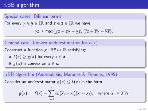
αBB algorithm

Special cases: Bilinear terms

For every y ∈ y ∈ IR and z ∈ z ∈ IR we have

yz ≥ max{yz + zy − yz, yz + zy − yz}.

General case: Convex underestimators for f (x)

Construct a function g : Rn 7→ R satisfying:

f (x) ≥ g(x) for every x ∈ x,

g(x) is convex on x ∈ x.

αBB algorithm (Androulakis, Maranas & Floudas, 1995)

Consider an underestimator g(x) ≤ f (x) in the form

g(x) := f (x)−n∑

i=1

αi (x i − xi )(xi − x i ), where αi ≥ 0 ∀i .

15 / 46

Illustration

−3−2

−10

12

3

−3−2

−10

12

3

−300

−200

−100

0

100

200

Function f (x) and its convex underestimator g(x).

16 / 46

Computation of α

Idea

The Hessian of g(x) reads

∇2g(x) = ∇2f (x) + 2 diag(α).

Choose α large enough to ensure positive semidefinitness of the Hessian of

g(x) := f (x)−∑ni=1 αi (x i − xi)(xi − x i).

Interval Hessian matrix

Let H be an interval matrix enclosing the image of ∇2f (x) over x ∈ x:

∂2

∂xi∂xjf (x) ∈ hij = [hij , hij ], ∀x ∈ x.

Remarks

Checking positive semidefiniteness of each H ∈ H is co-NP-hard.

Various enclosures for eigenvalues of H ∈ H.

Scaled Gerschgorin method enables to express αi -s.

17 / 46

Computation of α

Scaled Gerschgorin method for α

αi := max{0,−1

2

(hii −

∑j 6=i |hij |dj/di

)}, i = 1, . . . , n,

where |hij | = max{|hij |, |hij |

}.

To reflect the range of the variable domains, use d := x − x .

Theorem (H., 2014)

The choice d := x − x is optimal (i.e., it minimizes the maximumseparation distance between f (x) and g(x)) if

hiidi −∑

j 6=i |hij |dj ≤ 0, ∀i = 1, . . . , n.

18 / 46

Next Section



3 Convexification

4 Linearization



19 / 46

Linearization

Interval linear programming approach

linearize constraints,

compute new bounds and iterate.

Example

xx

S

x

S

x x′ ⊆ x

S

20 / 46

Mean value form

Theorem

Let f : Rn 7→ R, x ∈ IRn and a ∈ x. Then

f (x) ⊆ f (a) +∇f (x)T (x− a),

Proof.

By the mean value theorem, for any x ∈ x there is c ∈ x such that

f (x) = f (a) +∇f (c)T (x − a) ∈ f (a) +∇f (x)T (x− a).

Improvements

successive mean value form

f (x) ⊆ f (a) + f ′x1(x1, a2, . . . , an)(x1 − a1)

+ f ′x2(x1, x2, a3 . . . , an)(x2 − a2) + . . .

+ f ′xn(x1, . . . , xn−1, xn)(xn − an).

replace derivatives by slopes

21 / 46

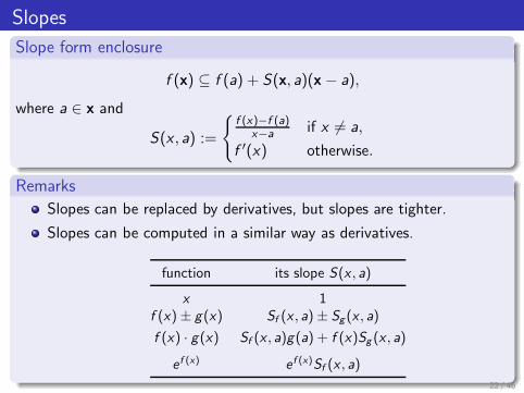
Slopes

Slope form enclosure

f (x) ⊆ f (a) + S(x, a)(x − a),

where a ∈ x and

S(x , a) :=

{f (x)−f (a)

x−a if x 6= a,

f ′(x) otherwise.

Remarks

Slopes can be replaced by derivatives, but slopes are tighter.

Slopes can be computed in a similar way as derivatives.

function its slope S(x , a)

x 1f (x)± g(x) Sf (x , a)± Sg (x , a)

f (x) · g(x) Sf (x , a)g(a) + f (x)Sg (x , a)

e f (x) e f (x)Sf (x , a)

22 / 46

Slopes

Example

f (x) = 14x

2 − x + 12 , x = [1, 7].

f ′(x) = [−12 ,

52 ], Sf (x, x

c) = [14 ,74 ].

1

2

3

4

5

1 2 3 4 5 6 7 8−1 0 x

y

f (x)

f ′(x)

Sf (x, xc )

23 / 46

Linearization

Interval linearization

Let x0 ∈ x. Suppose that a for some interval matrices A and B we have

h(x) ⊆ A(x − x0) + h(x0), ∀x ∈ x

g(x) ⊆ B(x − x0) + g(x0), ∀x ∈ x,

e.g., by the mean value form, slopes, . . .

Interval linear programming formulation

Now, the set S is enclosed by

A(x − x0) + h(x0) = 0,

B(x − x0) + g(x0) ≤ 0.

What remains to do

Solve the interval linear program

Choose x0 ∈ x

24 / 46

Linearization

Case x0 := x

Let x0 := x . Since x − x is non-negative, the solution set to

A(x − x0) + h(x0) = 0,

B(x − x0) + g(x0) ≤ 0,

is described by

Ax ≤ A x − h(x), Ax ≥ Ax − h(x),

Bx ≤ B x − g(x).

Similarly if x0 is any other vertex of x

25 / 46

Linearization

General case

Let x0 ∈ x. The solution set to

A(x − x0) + h(x0) = 0,

B(x − x0) + g(x0) ≤ 0,

is described by

|Ac(x − x0) + h(x0)| ≤ A∆|x − x0|,Bc(x − x0) + g(x0) ≤ B∆|x − x0|.

Non-linear description due to the absolute values.

How to get rid of them?

Estimate from above by a linear function: |x − x0| ≤ α(x − x0) + β.(Easy to find the best upper linear estimation.)

26 / 46

Linearization

Example

Typical situation when choosing x0 to be vertex:

x

x0

S

27 / 46

Linearization

Example

Typical situation when choosing x0 to be the opposite vertex:

x

x0

S

28 / 46

Linearization

Example

Typical situation when choosing x0 = xc :

x S

x0

29 / 46

Linearization

Example

Typical situation when choosing x0 = xc (after linearization):

x S

x0

30 / 46

Linearization

Example

Typical situation when choosing all of them:

x S

31 / 46

Next Section



3 Convexification

4 Linearization



32 / 46

Examples

Example (The COPRIN examples, 2007, precision ∼ 10−6)

tf12 (origin: COCONUT, solutions: 1, computation time: 60 s)

min x1 +12x2 +

13x3

s.t. − x1 − imx2 − ( i

m )2x3 + tan( im ) ≤ 0, i = 1, . . . ,m (m = 101).

o32 (origin: COCONUT, solutions: 1, computation time: 2.04 s)

min 37.293239x1 + 0.8356891x5x1 + 5.3578547x23 − 40792.141

s.t. −0.0022053x3x5 + 0.0056858x2x5 + 0.0006262x1x4 − 6.665593 ≤ 0,−0.0022053x3x5 − 0.0056858x2x5 − 0.0006262x1x4 − 85.334407 ≤ 0,

0.0071317x2x5 + 0.0021813x23 + 0.0029955x1x2 − 29.48751 ≤ 0,

−0.0071317x2x5 − 0.0021813x23 − 0.0029955x1x2 + 9.48751 ≤ 0,

0.0047026x3x5 + 0.0019085x3x4 + 0.0012547x1x3 − 15.699039 ≤ 0,−0.0047026x3x5 − 0.0019085x3x4 − 0.0012547x1x3 + 10.699039 ≤ 0.

Rastrigin (origin: Myatt (2004), solutions: 1 (approx.), time: 2.07 s)

min 10n+∑n

j=1(xj − 1)2 − 10 cos(2π(xj − 1)),

where n = 10, xj ∈ [−5.12, 5.12].33 / 46

Examples

One of the Rastrigin functions.

34 / 46

Software

Rigorous global optimization software

GlobSol (by R. Baker Kearfott), written in Fortran 95, open-sourceexist conversions from AMPL and GAMS representations,http://interval.louisiana.edu/

COCONUT Environment, open-source C++ classeshttp://www.mat.univie.ac.at/~coconut/coconut-environment/

GLOBAL (by Tibor Csendes), for Matlab / Intlab,free for academic purposeshttp://www.inf.u-szeged.hu/~csendes/linkek_en.html

PROFIL /BIAS (by O. Knuppel et al.), free C++ classhttp://www.ti3.tu-harburg.de/Software/PROFILEnglisch.html

See also

C.A. Floudas (http://titan.princeton.edu/tools/)

A. Neumaier (http://www.mat.univie.ac.at/~neum/glopt.html)

35 / 46

References

C. A. Floudas.Deterministic Global Optimization. Theory, Methods and Applications.Kluwer, Dordrecht, 2000.

C. A. Floudas and P. M. Pardalos, editors.Encyclopedia of Optimization. 2nd ed.Springer, New York, 2009.

E. R. Hansen and G. W. Walster.Global Optimization Using Interval Analysis.Marcel Dekker, New York, second edition, 2004.

R. B. Kearfott.Rigorous Global Search: Continuous Problems.Kluwer, Dordrecht, 1996.

A. Neumaier.Complete Search in Continuous Global Optimization and ConstraintSatisfaction.Acta Numerica, 13:271–369, 2004.

36 / 46

Next Section



3 Convexification

4 Linearization



37 / 46

AlgoIss: Global Optimization

Minimization of f (x1, . . . , xn) — usual testing functions:

Rastrigin’s function 20 + x21 + x22 − 10(cos 2πx1 + cos 2πx2)

Banana (Rosenbrock) function (1− x1)2 + 100(x2 − x21 )

2

hidden minimum function

−2

−1

0

1

2 −2

0

2

4

0

1000

2000

3000

4000

38 / 46

AlgoIss: Computation models

How to represent the function f ?

Special optimization problems: analytical expression (e.g.12x

THx + cTx + α for quadratic programming)

A general function: oracle model — there is a blackbox f s.t. on aquery x it returns f (x)

In the oracle model: complexity often measured by the number oforacle queries

Problem: How to measure the size of input?

39 / 46

AlgoIss: ExampleHidden-minimum function:

0

−1

ε

a

Theorem

There is no finite upper bound on the number of steps for an optimizationalgorithm to locate the global minimum.

Proof.

For a finite number of testing points, ε can be chosen so small so that thealgorithm cannot distinguish between the zero function and thehidden-minimum function.

40 / 46

AlgoIss: Further problems

Approximate solution

The minimizer may be irrational — a problem with representation bya Turing machine

Example: min{xTAx : xTx ≤ 1} = λmin(A) for A negative definite.The number λmin(A) is often irrational even for a rational matrix A;the minimizer is its corresponding eigenvector.

Possible solution: real-number computation model. [Drawback: welose finite-time convergence of many weakly polynomial methods,such as the Ellipsoid Method or IPMs.]

Another solution: find approximate optima.

41 / 46

AlgoIss: Approximate minimum

Definition

A point x is an ε-approximate minimum is f (x)− f (x∗) ≤ ε, where x∗ isthe true minimizer.

Remarks.

Weak definition — though f (x) is close to f (x∗), the distance‖x − x∗‖∞ can still be extremely large. So sometimes one also addsthe requirement: “. . . and ‖x − x∗‖∞ ≤ ε”.

This problem vanishes for Lipschitz functions.

Theorem

If f is L-Lipschitz, then the ε-approximate global minimum of f over a unitcube can be found in ≈ (12

Lε )

n steps and not faster.

42 / 46

AlgoIss: Approximate minimum (contd.)

Theorem

If f is L-Lipschitz, then the ε-approximate global minimum of f over theunit cube [0, e] can be found in ≈ (12

Lε )

n steps and not faster.

Proof idea.

Upper bound. Cover the cube [0, e] by a regular n-dimensional gridwith distance 2ε

L between neighbor points and evaluate f in each gridpoint; then take the minimum. Then ‖x − x∗‖∞ ≤ ε

L for some gridpoint x and f (x) − f (x∗) ≤ L‖x − x∗‖ ≤ ε.

Lower bound. Let ε′ > ε. Define a hidden-minimum function fv

fv (x) =

{0 if‖v − x‖∞ ≥ ε′

L ,

L‖v − x‖∞ − ε′ if‖v − x‖∞ < ε′L .

Then, v is the minimizer. Idea: any algorithm that uses less than(12

Lε )

n oracle queries to f leaves some region of [0, e] “uninspected”;so we can place v into that region. Thus the algorithm cannot find itand it cannot distinguish between fv and the zero function.

43 / 46

AlgoIss: Summary and special cases

In general, global minimization is nonrecursive (to recall: an algorithmfor the question “min f (x1, . . . , xn) ≤? 0” would solve Hilbert’s TenthProblem. This holds true even for the case n = 1.

So we must inspect the general problem by subcases.

Polynomials

Recursive by Tarski’s quantifier elimination, but extremely slow.

Idea: the question “does a given polynomial p(x1, . . . , xn) attain avalue f0?” can be written as an arithmetical formula

(∃x1) · · · (∃xn)p(x1, . . . , xn) = f0

& x1 ≤ x1 ≤ x1 & · · · & xn ≤ xn ≤ xn. (1)

Tarski proved that Theory of Real Closed Fields is decidable. So inprinciple, we can enumerate all proofs until we find a proof of (1) orits negation. This proves recursivity.

44 / 46


Convex optimization

“Nice” case: local minimum = global minimum

However, in general nothing can be proved without additionalassumptions

ε-approximate minimization of a differentiable convex L-Lipschitzfunction can be done in time O(n2(log n+ log L

ε )) in the oracle model

Further problems we must face: Example

Optimization under quadratic constraints xTHx + cTx ≤ γ — is thefeasibility problem in NP?

Problem: a feasible point cannot be used as an NP-witness, since itcan happen that bit-size of (a unique) feasible point is exponential inbitsize of H, c , γ.

45 / 46


Quadratic programming min xTHx + cTx s.t. Ax ≤ b

The convex case (H psd): polynomial time

A single eigenvalue of H is negative: NP-hard

H general: optimization over an ellipsoid: polynomial time

H general: optimization over a simplex: NP-hard

H general: “is given x a local minimum of xTHx + cTx?”: NP-hard

further results: the form min xTHx + cTx s.t. x ∈ x with H nsd of afixed rand: polynomial time

46 / 46

introduction to interval computation

Documents