introduction to dynamic programming applied to economics · 2.1.2 dynamic programming the principle...
TRANSCRIPT
Introduction to Dynamic ProgrammingApplied to Economics
Paulo BritoDepartamento de Economia
Instituto Superior de Economia e GestaoUniversidade Tecnica de Lisboa
27.9.2007

Contents
1 Introduction 31.1 A general overview . . . . . . . . . . . . . . . . . . . . . . . . . . 4
1.1.1 Discrete time deterministic models . . . . . . . . . . . . . 41.1.2 Continuous time deterministic models . . . . . . . . . . . . 51.1.3 Discrete time stochastic models . . . . . . . . . . . . . . . 51.1.4 Continuous time stochastic models . . . . . . . . . . . . . 6
1.2 References . . . . . . . . . . . . . . . . . . . . . . . . . . . . . . . 6
I Deterministic Dynamic Programming 7
2 Discrete Time 82.1 Optimal control and dynamic programming . . . . . . . . . . . . 8
2.1.1 The benchmark problem in macroeconomics . . . . . . . . 92.1.2 Dynamic programming . . . . . . . . . . . . . . . . . . . . 11
2.2 Applications . . . . . . . . . . . . . . . . . . . . . . . . . . . . . . 132.2.1 Representative agent problem . . . . . . . . . . . . . . . . 132.2.2 The Ramsey problem . . . . . . . . . . . . . . . . . . . . . 18
3 Continuous Time 203.1 The dynamic programming principle and the HJB equation . . . . 20
3.1.1 Simplest problem . . . . . . . . . . . . . . . . . . . . . . . 203.1.2 Infinite horizon discounted problem . . . . . . . . . . . . 233.1.3 Bibliography . . . . . . . . . . . . . . . . . . . . . . . . . . 24
3.2 Applications . . . . . . . . . . . . . . . . . . . . . . . . . . . . . . 243.2.1 The representative agent problem . . . . . . . . . . . . . . 243.2.2 The Ramsey model . . . . . . . . . . . . . . . . . . . . . . 28
II Stochastic Dynamic Programming 30
4 Discrete Time 314.1 Introduction to stochastic processes . . . . . . . . . . . . . . . . . 31
1

Paulo Brito Dynamic Programming 2007 2
4.1.1 Information structure . . . . . . . . . . . . . . . . . . . . . 314.1.2 Stochastic processes . . . . . . . . . . . . . . . . . . . . . 334.1.3 Probabilities and expectations . . . . . . . . . . . . . . . . 354.1.4 Particular stochastic processes . . . . . . . . . . . . . . . . 384.1.5 References . . . . . . . . . . . . . . . . . . . . . . . . . . . 38
4.2 Stochastic Dynamic Programming . . . . . . . . . . . . . . . . . . 394.3 Applications . . . . . . . . . . . . . . . . . . . . . . . . . . . . . . 41
4.3.1 The representative consumer . . . . . . . . . . . . . . . . . 41
5 Continuous time 455.1 Introduction to continuous time stochastic processes . . . . . . . . 45
5.1.1 Brownian motions . . . . . . . . . . . . . . . . . . . . . . . 455.1.2 Processes and functions of B . . . . . . . . . . . . . . . . . 465.1.3 Ito’s integral . . . . . . . . . . . . . . . . . . . . . . . . . . 485.1.4 Stochastic integrals . . . . . . . . . . . . . . . . . . . . . . 495.1.5 Stochastic differential equations . . . . . . . . . . . . . . . 515.1.6 Stochastic optimal control . . . . . . . . . . . . . . . . . . 53
5.2 The representative agent problem . . . . . . . . . . . . . . . . . . 555.3 A stochastic continous time DGE for asset prices . . . . . . . . . 58
5.3.1 Arrow-Debreu equilbrium . . . . . . . . . . . . . . . . . . 585.3.2 Finance economy . . . . . . . . . . . . . . . . . . . . . . . 60
5.4 Stochastic Ramsey model . . . . . . . . . . . . . . . . . . . . . . 62

Chapter 1
Introduction
We will study the two workhorses of modern macro and financial economics, usingdynamic programming methods:
• the intertemporal allocation problem for the representative agent in a fi-nance economy;
• the Ramsey model
in four different environments:
• discrete time and continuous time;
• deterministic and stochastic
methodology
• we use analytical methods
• some heuristic proofs
• and derive explicit equations whenever possible.
3

Paulo Brito Dynamic Programming 2007 4
1.1 A general overview
We will consider the following types of problems:
1.1.1 Discrete time deterministic models
In the space of the sequences ut, xt∞t=0, such that ut ∈ Rm where t → ut and
xt ∈ R where t → xt choose a sequence u∗t , x
∗t∞t=0 that maximizes the sum
maxu
∞∑t=0
βtf(ut, xt)
subject to the sequence of budget constraints
xt+1 = g(xt, ut), t = 0, ..,∞x0 given
where 0 < β ≡ 11+ρ
< 1, where ρ > 0.
By applying the principle of dynamic programming the first order nec-essary conditions for this problem are represented by the Hamilton-Jacobi-Bellman (HJB) equation,
V (xt) = maxut
f(ut, xt) + βV (g(ut, xt))
which is usually written as
V (x) = maxu
f(u, x) + βV (g(u, x)) (1.1)
If we can find the optimal control as u∗ = h(x), where h(x) is called thepolicy function, then solving the HJB equation means finding the functionV (x) which solves the functional equation
V (x) = f(h(x), x) + βV [g(h(x), x)].
Only in very rare cases we can find V (.) explicitly.
Paulo Brito Dynamic Programming 2007 5
1.1.2 Continuous time deterministic models
In the space of (piecewise-)continuous functions of time (u(t), x(t)) where t ∈ R+
choose an optimal flow (u∗(t), x∗(t)) such that u∗(t) maximizes the functional
V [u] =
∫ ∞
0
f(u(t), x(t))e−ρtdt
where ρ > 0 such that the instantaneous budget constraint and the initial state
dx
dt≡ x(t) = g(x(t), u(t)), t ≥ 0
x(0) = x0 given
hold.
By applying the principle of the dynamic programming the first order condi-tions of this problem solve the HJB equation
ρV (x) = maxu
f(u, x) + V
′(x)g(u, x)
1.1.3 Discrete time stochastic models
The variables are random sequences ut(ω), xt(ω)∞t=0 which are adapted to F =Ft∞t=0. The domain of the variables is ω ∈ (Ω,F , P, F)×N, such that (t, ω) → ut
and xt ∈ R where (t, ω) → xt. Then ut ∈ R is a random variable.An economic agent chooses a random sequence u∗
t , x∗t∞t=0 that maximizes the
sum
maxu
E0
[ ∞∑t=0
βtf(ut, xt)
]
subject to the contingent sequence of budget constraints
xt+1 = g(xt, ut, ωt+1), t = 0..∞,
x0 given
where 0 < β < 1.By applying the principle of the dynamic programming the first order condi-
tions of this problem solve the HJB equation
V (xt) = maxu
f(ut, xt) + βEt[V (g(ut, xt, ωt+1))]
where Et[V (g(ut, xt, ωt+1))] = E[V (g(ut, xt, ωt+1))|Ft]
Paulo Brito Dynamic Programming 2007 6
1.1.4 Continuous time stochastic models
In the space of the flows u(ω, t), x(ω, t) : ω = ω(t) ∈ (Ω,F , P,F(t)), t ∈ R+choose a flow u∗(t) that maximizes the functional
V [u] = E0
[∫ ∞
0
f(u(t), x(t))e−ρtdt
]
where u(t) = u(ω(t), t) and x(t) = x(ω(t), t) are Itprocesses and ρ > 0 such thatthe instantaneous budget constraint is represented by a stochastic differentialequation
dx = g(x(t), u(t), t)dt + σ(x(t), u(t))dB(t), t ∈ R+
x(0) = x0 given
where dB(t) is a Wiener process.
By applying the stochastic version of the principle of DP the HJB equation is
ρV (x) = maxu
f(u, x) + g(u, x)V
′(x) +
1
2(σ(u, x))2V
′′(x)
.
1.2 References
First contribution: Bellman (1957)Discrete time: Bertsekas (1976), Sargent (1987), Stokey and Lucas (1989),
Ljungqvist and Sargent (2000)Continous time: Fleming and Rishel (1975), Kamien and Schwartz (1991)
Part I
Deterministic DynamicProgramming
7
Chapter 2
Discrete Time
2.1 Optimal control and dynamic programming
General description of the optimal control problem:
• assume that time evolves in a discrete way, meaning that t ∈ 0, 1, 2, . . .,that is t ∈ N0;
• the economy is described by two variables that evolve along time: a statevariable xt and a control variable, ut;
• we know the initial value of the state variable, x0, and the law of evolutionof the state, which is a function of the control variable (u(.)): xt+1 =gt(xt, ut);
• we assume that the controls belong to a set ut ∈ U for any t ∈ N,
• then, for any sequence of controls, u
u ≡ u0, u1, . . . : ut ∈ Uthe economy can follow a large number of feasible paths, x can be followedwhere
x ≡ x0, x1, . . ., where xt+1 = gt(xt, ut) ut ∈ U• however, if we have a criteria that allows for the evaluation of all feasible
pathsU(x0, x1, . . . , u0, u1, . . .)
• and if there is at least an optimal control u∗ = u∗0, u
∗1, . . . which maximizes
U ,
• then there is at least an optimal path for the state variable
x∗ ≡ x0, x∗1, . . .
8

9
2.1.1 The benchmark problem in macroeconomics
Assumptions:
• timing: the state variable xt is usually a stock and is measured at thebeginning of period t and the control ut is usually a flow and is measuredin the end of period t;
• horizon: can be finite or is infinite (T = ∞). The second case is morecommon;
• objective functional:- there is an intertemporal utility function is additively separable, station-ary, and involves time-discounting (impatience):
T∑t=0
βtf(ut, xt), 0 < β < 1
- f(.) is well behaved: continuous, continuously differentiable and concave;
• the economy is described by an autonomous difference equation
xt+1 = g(xt, ut)
where g(.) is autonomous, continuous, differentiable, concave. Then the DEverifies the conditions for existence and uniqueness of solutions;
• the non-Ponzi game condition holds:
limt→∞
ϕtxt ≥ 0
holds, for a discount factor 0 < ϕ < 1;
• there may be some side conditions, v.g., xt ≥ 0, ut ≥ 0, which may producecorner solutions. We will deal only with the case in which the solutions areinterior (or the domain of the variables is open).
10
The optimal control problem (OCP) :
Find u∗t , xt∞t=0: which solves
maxut∞t=0
∞∑t=0
βtf(ut, xt)
such that ut ∈ U andxt+1 = g(xt, ut)
for x0 given.
Feasible candidate solutions: paths of xt, ut that verify
xt+1 = g(xt, ut), x0 given
for any choice of ut ∈ U∞t=0.
Methods for solving the OCP in the sense of obtaining necessary condi-tions or necessary and sufficient conditions:
• method of Lagrange (for the case T finite)
• Pontriyagin’s maximum principle
• dynamic programming principle.
Necessary and sufficient optimality conditions
• necessary conditions: assuming that we know the optimal solution, u∗t , x
∗t
which conditions should the variables of the problem verify ? (This meansthat they hold for every extremum feasible solutions);
• sufficient conditions: if the functions defining the problem verify some con-ditions, then feasible paths verifying some conditions are solutions of theproblem.
In general, if the behavioral functions f(.) and g(.) are well behaved (contin-uous, continuously differentiable and concave) then necessary conditions are alsosufficient.

11
2.1.2 Dynamic programming
The Principle of the dynamic programming (Bellman (1957)):an optimal trajectory has the following property:for any given initial values of the state variable and for a given value of the stateand control variables in the beginning of any period, the control variables shouldbe chosen optimally for the remaining period, if we take the optimal values ofthe state variables which result from the previous optimal decisions.
We next follow an heuristic approach for deriving necessary conditions follow-ing the principle of DP.
Finite horizon Assume that we know a solution optimal control u∗, x∗tT
t=0.Which properties has the optimal solution ?
Definition: value function at time τ
VT−τ (xτ ) =
T∑τ=t
βt−τf(u∗τ , x
∗τ )
Then, for time τ = 0 we have
VT (x0) = maxutT
t=0
T∑t=0
βtf(ut, xt) =
= maxutT
t=0
(f(x0, u0) + βf(x1, u1) + β2f(x2, u2) + . . .
)=
= maxutT
t=0
(f(x0, u0) + β
T∑t=1
βt−1f(xt, ut)
)=
= maxu0
(f(x0, u0) + β max
utTt=1
T∑t=1
βt−1f(xt, ut)
)
by the principle of dynamic programming.Then
VT (x0) = maxu0
f(x0, u0) + βVT−1(x1)We can apply the same idea for the value function for any time 0 ≤ t ≤ T to getthe Hamilton-Jacobi-Equation
VT−t(xt) = maxut
f(xt, ut) + βVT−t−1(xt+1) (2.1)
which holds for feasible solutions, i.e., verifying xt+1 = g(xt, ut) and given x0.
12
Proposition: given an optimal solution to the optimal control problem thenit verifies the HJB equation.
Intuition: we transform the maximization of a functional into a recursivetwo-period problem. We solve the control problem by solving the HJB equation.To do this we have to find VT , . . . , V0, through the recursion
Vt+1(x) = maxu
f(x, u) + βVt(g(x, u)) (2.2)
Infinite horizon For the infinite horizon discounted optimal control problem,the limit function V = limj→∞ Vj is independent of j so the Hamilton JacobiBellman equation becomes
V (x) = maxu
f(x, u) + βV [g(x, u)] = maxu
H(x, u)
Properties of the value function: it usually hard to get the properties ofV (.). In general continuity is assured but not differentiability (this is a subjectfor advanced courses on DP, see Stokey and Lucas (1989)).
If some regularity conditions hold, we may determine the optimal controlthrough the optimality condition
∂H(x, u)
∂u= 0
if H(.) is C2 then we get the policy function
u∗ = h(x)
which gives an optimal rule for changing the optimal control, given the state ofthe economy. If we can determine (or prove that there exists such a relationship)then we say that our problem is recursive.
In this case the HJB equation becomes a non-linear ODE
V (x) = f(x, h(x)) + βV [g(x, h(x))].
Solving the HJB: means finding the value function V (x). Methods: ana-lytical (in some cases exact) and mostly numerical (value function iteration).

13
2.2 Applications
2.2.1 Representative agent problem
Assumptions:
• there are T > 1 periods;
• consumers are homogeneous and have an additive intertemporal utilityfunctional;
• the instantaneous utility function is continuous, differentiable, increasing,concave and is homogenous of degree n;
• consumers have a stream of endowments, y ≡ ytTt=0, known with certainty;
• institutional setting: there are spot markets for the good and for a financialasset. The financial asset is an entitlement to receive the dividend Dt atthe end of every period t. The spot prices are Pt and St for the good andfor the financial asset, respectively.
• Market timing, we assume that the good market opens in the beginningand that the asset market opens at the end of every period.
The consumer’s problem
• choose a sequence of consumption ctTt=0 and of portfolios θtT
t=1, whichis, in this simple case, the quantity of the asset bought at the beginning oftime t, in order to find
maxct,θt+1T
t=0
T∑t=0
βtu(ct)
• subject to the sequence of budget constraints:
A0 + y0 = c0 + θ1S0
θ1(S1 + D1) + y1 = c1 + θ2S1
. . .
θt(St + Dt) + yt = ct + θt+1St
. . .
θT (ST + DT ) + yT = cT
where At is the stock of financial wealth (in real terms) at the beginning ofperiod t.

14
If we denoteAt+1 = θt+1St
then the generic period budget constraint as
At+1 = yt − ct + RtAt, t = 0, . . . , T (2.3)
where the asset return is
Rt+1 = 1 + rt+1 =St+1 + Dt+1
St.
Then the HJB equation is
V (At) = maxct
u(ct) + βV (At+1) (2.4)
To prove this, assume that we know the optimal solution for the consumer prob-lem c∗t , atT
t=0. For any moment t, define the value function as
V (At) =
T∑s=t
βs−tu(c∗s) = maxcsT
s=t
T∑s=t
βs−tu(cs)
from the principle of the dynamic programming
maxcsT
s=t
T∑s=t
βs−tu(cs) = maxct
u(ct) + max
csTs=t+1
(β
T∑s=t+1
βs−(t+1)u(cs)
)
then we get equation (2.4).We can write equation (2.4) as
V (A) = maxc
u(c) + βV (A)
(2.5)
where A = y − c + RA then V (A) = V (y − c + RA).
Deriving an intertemporal arbitrage condition
The optimality condition is:
u′(c∗) = βV
′(A)
if we could find the optimal policy function c∗ = h(A) and substitute it in theHJB equation we would get
V (A) = u(h(A)) + βV (A∗), A∗ = y − h(A) + RA.

15
Using the Benveniste and Scheinkman (1979) trick , we differentiate for A to get
V′(A) = u
′(c∗)
∂h
∂A+ βV
′(A∗)
∂A∗
∂A=
= u′(c∗)
∂h
∂A+ βV
′(A∗)
(R − ∂h
∂A
)=
= βRV′(A∗) =
= Ru′(c∗)
from the optimality condition. If we shift both members of the last equation weget
V′(A∗) = Ru
′(c∗),
and, thenRu
′(c∗) = β−1u
′(c∗).
Then, the optimal consumption path (we delete the * from now on) verifies thearbitrage condition
u′(c) = βRu
′(c)
oru
′(ct) = βu
′(ct+1)Rt (2.6)
Observe that
βRt =1 + rt
1 + ρ
the ratio between the market return and the psychological factor.If the utility function is homogenous of degree η, it has the properties
u(c) = cηu(1)
u′(c) = cη−1u
′(1)
the arbitrage condition is a linear difference equation
ct+1 = λct, λ ≡ (βRt)1
1−η
Determining the optimal value function
In some cases, we can get an explicit solution for the HJB equation (2.5). Wehave to determine jointly the optimal policy function h(A) and the optimal valuefunction V (A).
We will use a common non-constructive method to derive both functions:first, we make a conjecture on the form of V (.) and then apply the method of theundetermined coefficients.
16
Assumptions Let us assume that the utility function is logarithmic: u(c) =ln(c) and assume for simplicity that y = 0.
In this case the optimality condition becomes
c∗ = [βV′(RA − c∗)]−1
Conjecture: let us assume that the value function is of the form
V (x) = B0 + B1 ln(A) (2.7)
where B0 and B1 are undetermined coefficients.From this point on we apply the method of the undetermined coeffi-
cients: if the conjecture is right then we will get an equation without the inde-pendent variable x, and which would allow us to determine the coefficients, B0
and B1, as functions of the parameters of the HJB equation.
Then
V′=
B1
A.
Applying this to the optimality condition, we get
c∗ = h(A) =RA
1 + βB1
then
A∗ = RA − c∗ =
(βB1
1 + βB1
)RA
which is a linear function of A.
Substituting in the HJB equation, we get
B0 + B1 ln(A) = ln
(RA
1 + βB1
)+ β
[B0 + B1 ln
(βB1RA
1 + βB1
)]= (2.8)
= ln
(R
1 + βB1
)+ ln(A) + β
[B0 + B1 ln
(βB1R
1 + βB1
)+ ln(A)
]
The term in ln(A) can be eliminated if B1 = 1 + βB1, that is if
B1 =1
1 − β
and equation (2.8) reduces to
B0(1 − β) = ln(R(1 − β)) +β
1 − βln(Rβ)

17
which we can solve for B0 to get
B0 = (1 − β)−2 ln(RΘ), where Θ ≡ (1 − β)1−βββ
Finally, as our conjecture proved to be right, we can substitute B0 and B1 inequation (2.7) the optimal value function and the optimal policy function are
V (A) = (1 − β)−1 ln((RΘ)(1−β)−1
A)
andc∗ = (1 − β)RA
then optimal consumption is linear in financial wealth.We can also determine the optimal asset accumulation, by noting that ct = c∗
and substituting in the period budget constraint
At+1 = βRtAt
If we assume that Rt = R then the solution for that DE is
At = (βR)tA0, t = 0, . . . ,∞
and, therefore the optimal path for consumption is
ct = (1 − β)βtRt+1A0
Observe that the transversality condition holds,
limt→∞
R−tAt = limt→∞
A0βt = 0
because 0 < β < 1.
Exercises
1. solve the HJB equation for the case in which y > 0
2. solve the HJB equation for the case in which y > 0 and the utility functionis CRRA: u(c) = c1−θ/(1 − θ) , for θ > 0;
3. try to solve the HJB equation for the case in which y = 0 and the utilityfunction is CARA: u(c) = B − e−βc/β, for β > 0
4. try to solve the HJB equation for the case in which y > 0 and the utilityfunction is CARA: u(c) = B − e−βc/β, for β > 0.

18
2.2.2 The Ramsey problem
Find a sequence ct, kt∞t=0 which solves the following optimal control problem:
maxc∞t=0
∞∑t=0
βtu(ct)
subject tokt+1 = f(kt) − ct + (1 − δ)kt
where 0 ≤ δ ≤ 1 given k0. Both the utility function and the production functionare neoclassical: continuous, differentiable, smooth and verify the Inada condi-tions. These conditions would ensure that the necessary conditions for optimalityare also sufficient.
The HJB function is
V (k) = maxc
u(c) + βV (k
′)
where k′= f(k) − c + (1 − δ)k.
The optimality condition is
u′(c) = V
′(k
′(k))
If it allows us to find a policy function c = h(k) then the HJB becomes
V (k) = u[h(k)] + βV [f(k) − h(k) + (1 − δ)k] (2.9)
This equation has no explicit solution for generic utility and production function.Even for explicit utility and production functions the HJB has not an explicitsolution. Next we present a benchmark case where we can find an explicit solutionfor the HJB equation.
Benchmark case: Let u(c) = ln(c) and f(k) = Akα for 0 < α < 1, andδ = 1.
Conjecture:V (k) = B0 + B1 ln(k)
In this case the optimality condition is
h(k) =Akα
1 + βB1
If we substitute in equation (2.9) we get
B0 + B1 ln(k) = ln
(Akα
1 + βB1
)+ β
[B0 + B1 ln
(AkαβB1
1 + βB1
)](2.10)

19
Again we can eliminate the term in ln(k) by making
B1 =α
1 − αβ
Thus, (2.10) changes to
B0(1 − β) = ln(A(1 − αβ)) +αβ
1 − αβln(αβA)
Finally the optimal value function and the optimal policy function are
V (A) = (1 − αβ)−1 ln((AΘ)(1−β)−1
A)
, Θ ≡ (1 − αβ)1−αβ(αβ)αβ
andc∗ = (1 − αβ)Akα
Then the optimal capital accumulation is governed by the equation
kt+1 = αβAkαt
This equation generates a forward path starting from the known initial capitalstock k0
k0, αβAkα0 , (αβA)α+1kα2
0 , . . . , (αβA)αt−1+1kαt
0 , . . .which converges to a stationary solution: k = (αβA)1/(1−α).
Chapter 3
Continuous Time
3.1 The dynamic programming principle and the
HJB equation
3.1.1 Simplest problem
In the space of the functions (u(t), x(t)) for t0 ≤ t ≤ t1 find functions (u∗(t), x∗(t))which solve the problem:
maxu(t)
∫ t1
t0
f(t, x(t), u(t))dt
subject to
x ≡ dx(t)
dt= g(t, x(t), u(t))
given x(t0) = x0. We assume that t1 is know and that x(t1) is free.
The value function is, for the initial instant
V(t0, x0) =
∫ t1
t0
f(t, x∗, u∗)dt
and for the terminal time V(t1, x(t1)) = 0.
20

21
Lemma 1. First order necessary conditions for optimality from theDynamic Programming principleLet V ∈ C2(T, R). Then the value function which is associated to the optimal path(x∗(t), u∗(t) : t0 ≤ t ≤ t1 verifies the fundamental partial differential equationor the Hamilton-Jacobi-Bellman equation
−Vt(t, x) = maxu
[f(t, x, u) + Vx(t, x)g(t, x, u)].
Proof. Consider the value function
V(t0, x0) = maxu
(∫ t1
t0
f(t, x, u)dt
)
= maxu
(∫ t0+∆t
t0
f(.)dt +
∫ t1
t0+∆t
f(.)dt
)= (∆t > 0, small)
= maxu
t0 ≤ t ≤ t0 + ∆t
∫ t0+∆t
t0
f(.)dt + maxu
t0 + ∆t ≤ t ≤ t1
(∫ t1
t0+∆t
f(.)dt
) =
(from dynamic prog principle)
= maxu
t0 ≤ t ≤ t0 + ∆t
[∫ t0+∆t
t0
f(.)dt + V(t0 + ∆t, x0 + ∆x)
]=
(approximating x(t0 + ∆t) ≈ x0 + ∆x)
= maxu
t0 ≤ t ≤ t0 + ∆t
[f(t0, x0, u)∆t + V(t0, x0) + Vt(t0, x0)∆t + Vx(t0, x0)∆x + h.o.t]
if u ≈ constant and V ∈ C2(T, R)). Passing V(t0, x0) to the second member,dividing by ∆t and taking the limit lim∆t→0 we get, for every t ∈ [t0, t1],
0 = maxu
[f(t, x, u) + Vt(t, x) + Vx(t, x)x].

22
Observations:
• In the DP theory the function u∗ = h(t, x) is called the policy function .Then the HJB equation may be written as
−Vt(t, x) = f(t, x, h(t, x)) + Vx(t, x)g(t, x, h(t, x))].
• Though the differentiability of V is assured for the functions f and g whichare common in the economics literature, we can get explicit solutions, forV (.) and for h(.), only in very rare cases. Proving that V is differentiable,even in the case in which we cannot determine it explicitly is hard andrequires proficiency in Functional Analysis.
Relationship with the Pontriyagin’s principle:
(1) If we apply the transformation λ(t) = Vx(t, x(t)) we get the following rela-tionship with the Hamiltonian function which is used by the Pontriyagin’sprinciple: −Vt(t, x) = H∗(t, x, λ);
(2) If V is sufficienty differentiable, we can use the principle of DP to getnecessary conditions for optimality similar to the Pontriyagin principle.The maximum condition is
fu + Vxgu = fu + λgu = 0
and the canonical equations are: as λ = ∂Vx
∂t= Vxt + Vxxg and differenting
the HJB as regards x, implies −Vtx = fx + Vxxg + Vxgx, therefore thecanonical equation results
−λ = fx + λgx.
(3) Differently from the Pontryiagin’s principle which defines a dynamic systemof the form T, R2, ϕt = (q(t), x(t)), the principle of dynamic programmingdefines a dynamic system as (T, R), R, vt,x = V(t, x)). That is, if definesa recursive mechanism in all or in a subset of the state space.

23
3.1.2 Infinite horizon discounted problem
Lemma 2. First order necessary conditions for optimality from the Dy-namic Programming principleLet V ∈ C2(T, R). Then the value function associated to the optimal path (x∗(t), u∗(t) :t0 ≤ t < +∞ verifies the fundamental non-linear ODE called the Hamilton-Jacobi-Bellman equation
ρV (x) = maxu
[f(x, u) + V ′(x)g(x, u)].
Proof. Now, we have
V(t0, x0) = maxu
(∫ +∞
t0
f(x, u)e−ρtdt
)=
= e−ρt0 maxu
(∫ +∞
t0
f(x, u)e−ρ(t−t0)dt
)=
= e−ρt0V (x0) (3.1)
where V (.) is independent from t0 and only depends on x0. We can do
V (x0) = maxu
(∫ +∞
0
f(x, u)e−ρtdt
).
If we let, for every (t, x) V(t, x) = e−ρtV (x) and if we substitute the derivativesin the HJB equation for the simplest problem, we get the new HJB.
Observations:
• if we determine the policy function u∗ = h(x) and substitute in the HJBequation, we see that the new HJB equation is a ODE of the type x(t) =a(t) + b(t)x(t). This new HJB defines a recursion over x. Intuitively itgenerates a rule which says : if we observe the state x the optimal policyis h(x) in such a way that the initial value problem should be equal to thepresent value of the variation of the state.
• It is still very rare to find explicit solutions for V (x). There is a literature onhow to compute it numerically, which is related to the numerical solution ofODE’s and not with approximating value functions as in the discrete timecase.
24
3.1.3 Bibliography
See Kamien and Schwartz (1991).
3.2 Applications
3.2.1 The representative agent problem
Assumptions:
• T = R+, i.e., decisions and transactions take place continuously in time,and variables are represented by flows or trajectories x ≡ x(t), t ∈ R+where x(t) is a mapping t → x(t);
• deterministic environment: the agents have perfect information over theflow of endowments y ≡ y(t), t ∈ R+ and the relevant prices;
• agents are homogeneous: they have the same endowments and preferences;
• preferences over flows of consumption are evaluated by the intertemporalutility functional
V [c] =
∫ ∞
0
u(c(t))e−ρtdt
which displays impatience (the discount factor e−ρt ∈ (0, 1)), stationarity(u(.) is not directly dependent on time) and time independence and theinstantaneous utility function (u(.)) is continuous, differentiable, increasingand concave;
• observe that mathematically the intertemporal utility function is in fact afunctional, or a generalized function, i.e., a mapping whose argument is afunction (not a number as in the case of functions). Therefore, solving theconsumption problem means finding an optimal function. In particular, itconsists in finding an optimal trajectory for consumption;
• institutional setting: there are spot real and financial markets that arecontinuously open. The price P (t) clear the real market instantaneously.There is an asset market in which a single asset is traded which has theprice S(t) and pays a dividend V (t).
Derivation of the budget constraint:
The consumer chooses the number of assets θ(t). If we consider a smallincrement in time h and assume that the flow variables are constant in the intervalthen
S(t + h)θ(t + h) = θ(t)S(t) + θ(t)D(t)h + P (t)(y(t) − c(t))h.

25
Define A(t) = S(t)θ(t) in nominal terms.The budget constraint is equivalently
A(t + h) − A(t) = i(t)A(t)h + P (t)(y(t) − c(t))h
where i(t) = D(t)S(t)
is the nominal rate of return. If we divide by h and take thelimit when h → 0 then
limh→0
A(t + h) − A(t)
h≡ dA(t)
dt= i(t)A(t) + P (t)(y(t) − c(t)).
If we define real wealth and the real interest rate as a(t) ≡ A(t)P (t)
and r(t) =
i(t) + PP (t)
, then we get the instantaneous budget constraint
a(t) = r(t)a(t) + y(t) − c(t) (3.2)
where we assume that a(0) = a0 given.
Define the human wealth, in real terms, as
h(t) =
∫ ∞
t
e−R s
t r(τ)dτy(s)ds
as from the Leibniz’s rule
h(t) ≡ dh(t)
dt= r(t)
∫ ∞
t
e−R st r(τ)dτy(s)ds − y(t) = r(t)h(t) − y(t)
then total wealth at time t is
w(t) = a(t) + h(t)
and we may represent the budget constraint as a function of w(.)
w = a(t) + h(t) =
= r(t)w(t) − c(t)
The instantaneous budget constraint should not be confused with the in-tertemporal budget constraint. Assume the solvalibity condition holds attime t = 0
limt→∞
e−R t0
r(τ)dτa(t) = 0.
Then it is equivalent to the following intertemporal budget constraint,
w(0) =
∫ ∞
0
e−R t0 r(τ)dτ c(t)dt,
26
the present value of the flow of consumption should be equal to the initial totalwealth.
To prove this, solve the instantaneous budhet constraint (3.2) to get
a(t) = a(0)eR t0 r(τ)dτ +
∫ t
0
eR s0 r(τ)dτy(s) − c(s)ds
multiply by e−R t0
r(τ)dτ , pass to the limit t → ∞, apply the solvability conditionand use the definition of human wealth.
Therefore the intertemporal optimization problem for the represen-tative agent is to find (c∗(t), w∗(t)) for t ∈ R+ which maximizes
V [c] =
∫ +∞
0
u(c(t))e−ρtdt
subject to the instantaneous budget constraint
w(t) = r(t)w(t) − c(t)
given w(0) = w0.
Solving the consumer problem using DP.
The HJB equation is
ρV (w) = maxc
u(c) + V
′(w)(rw − c)
where w = w(t), c = c(t), r = r(t).
We assume that the utility function is homogeneous of degree η. Therefore ithas the properties:
u(c) = cηu(1)
u′(c) = cη−1u
′(1)
The optimality condition is:
u′(c∗) = V
′(w)
then
c∗ =
(V
′(w)
u′(1)
) 1η−1
27
substituting in the HJB equation we get the ODE, defined on V (w),
ρV (w) = rwV′(w) + (u(1) − u
′(1))
(V
′(w)
u′(1)
) ηη−1
In order to solve it, we guess that its solution is of the form:
V (w) = Bwη
if we substitute in the HJB equation, we get
ρBwη = ηrBwη + (u(1) − u′(1))
(ηBw
u′(1)
)η
.
Then we can eliminate the term in wη and solve for B to get
B =
[(u(1) − u
′(1)
ρ − ηr
)(η
u′(1)
)η] 11−η
.
Then, as B is a function of r = r(t), we determine explicitly the value function
V (w(t)) = B(t)w(t)η =
[(u(1) − u
′(1)
ρ − ηr(t)
)(η
u′(1)
)η] 11−η
w(t)η
as a function of total wealth.Observation: this is one know case in which we can solve explicitly the
HJB equation as it is a linear function on the state variable, w and the objectivefunction u(c) is homogeneous.
The optimal policy function can also be determined explicitly
c∗(t) =
(ηB(t)
u′(1)
) 1η−1
w(t) ≡ π(t)w(t) (3.3)
as it sets the control as a function of the state variable, and not as depending onthe path of the co-state and state variables as in the Pontryiagin’s case, sometimesthis solution is called robust feedback control.
Substituting in the budget constraint, we get the optimal wealth accumulation
w∗(t) = w0eR t0
r(s)−π(s)ds (3.4)
which is a solution of
w∗ = r(t)w∗(t) − c∗(t) = (r(t) − π(t))w∗(t)
Conclusion: the optimal paths for consumption and wealth accumulation (c∗(t), w∗(t))are given by equations (3.3) and (3.4) for any t ∈ R+.

28
3.2.2 The Ramsey model
Brock and Mirman (1972) This is a problem for a centralized planner whichchooses the optimal consumption flow c(t) in order to maximize the intertemporalutility functional
max V [c] =
∫ ∞
0
u(c)e−ρtdt
where ρ > 0 subject to
k(t) = f(k(t)) − c(t)
k(0) = k0 given
The HJB equation is
ρV (k) = maxc
u(c) + V′(k)(f(k) − c)
Benchmark assumptions: u(c) = c1−σ
1−σwhere σ > 0 and f(k) = Akα where
0 < α < 1.
The HJB equation is
ρV (k) = maxc
c1−σ
1 − σ+ V
′(k) (Akα − c)
(3.5)
the optimality condition is
c∗ =(V
′(k))− 1
σ
after substituting in equation (3.5) we get
ρV (k) = V′(k)
(σ
1 − σV
′(k)−
1σ + Akα
)(3.6)
In some particular cases we can get explicit solutions, but in general we don’t.
Particular case: α = σ Equation (3.6) becomes
ρV (k) = V′(k)
(σ
1 − σV
′(k)−
1σ + Akσ
)(3.7)
Let us conjecture that the solution is
V (k) = B0 + B1k1−σ
where B0 and B1 are undetermined coefficients. Then V′(k) = B1(1 − σ)k−σ.
29
If we substitute in equation (3.7) we get
ρ(B0 + B1k1−σ) = B1
[σ ((1 − σ)B1)
− 1σ k1−σ + (1 − σ)A
](3.8)
Equation (3.8) is true only if
B0 =A(1 − σ)
ρB1 (3.9)
B1 =
(1
1 − σ
)(σ
ρ
)σ
. (3.10)
Then the following function is indeed a solution of the HJB equation in thisparticular case
V (k) =
(σ
ρ
)σ (A
ρ+
1
1 − σk1−σ
)The optimal policy function is
c = h(k) =ρ
σk
We can determine the optimal flow of consumption and capital (c∗(t), k∗(t))by substituting c(t) = ρ
σk(t) in the admissibility conditions to get the ODE
k∗ = Ak∗(t)α − ρ
σk∗(t)
for given k(0) = k0. This a Bernoulli ODE which has an explicit solution as
k∗(t) =
[Aρ
σ+
(k
11−σ
0 − Aρ
σ
)e−
(1−σ)ρσ
t
] 11−σ
, t = 0, . . . ,∞
andc∗(t) =
ρ
σk∗(t), t = 0, . . . ,∞.

Part II
Stochastic DynamicProgramming
30

Chapter 4
Discrete Time
4.1 Introduction to stochastic processes
Assume that we have T periods: T = 0, 1, . . . , T and a probability space(Ω,F , P ) with a finite number of states of nature Ω = ω1, . . . , ωN. N =number of the states of nature.
The information available at period t ∈ T will be represented by the σ−algebraFt ⊂ F .
4.1.1 Information structure
Let the information be represented by the random sequence of events wtTt=0
belonging to a sequence of elements of Ω, Ft.If we consider the set of all the states of nature in each period, we may
establish a (one to one) correspondence between the sequences of informationand the sequences of partitions, P0,P1, . . . ,PT , over Ω, where
• P0 = Ω;
• the elements of Pt are mutually disjoint and are equivalent to the union ofelements of Pt+1;
• PT = ω1, ω2, . . . , ωN.The time sequence of events is wt ∈ Pt.
Example (vd Pliska (1997)) Let N = 8, T = 3, a admissible sequence ofpartitions is:
P0 = w0 = ω1, ω2, ω3, ω4, ω5, ω6, ω7, ω8P1 = w1
1, w12 = ω1, ω2, ω3, ω4, ω5, ω6, ω7, ω8
P2 = w21, w
22, w
23, w
24 = ω1, ω2, ω3, ω4, ω5, ω6, ω7, ω8
P3 = w31, w
32, . . . , w
38 = ω1, ω2, ω3, ω4, ω5, ω6, ω7, ω8
31
32
We may understand those partitions as sequences of two states of nature, agood state u and a bad state d. Then: ω1 = uuu, ω2 = uud, ω3 =udu, ω4 = udd, ω5 = duu, ω6 = dud, ω7 = ddu and ω8 = ddd,ω1, ω2 = uu, ω3, ω4 = ud, ω5, ω6 = du, ω7, ω8 = dd, ω1, ω2, ω3, ω4 = uand ω5, ω6, ω7, ω8 = d and ω1, ω2, ω3, ω4, ω5, ω6, ω7, ω8 = u, d.
If we define Nt as the number of elements of the partition Pt then wt ∈wt
sNts=1.
Given a partition, we may obtain as many subsets as possible, by means ofset operations (complements, unions and intersections) and build a σ−algebra.There is, therefore, a correspondence between sequences of partitions over Ω andsequences σ−algebras Ft ⊂ F .
The information available at time t ∈ T will be represented by Ft and by afiltration, for the sequence of periods t = 0, 1, . . . , T .
Definition 1. A filtration is a sequence of σ−algebras FtF = F0,F1, . . . ,FT.
A filtration is non-anticipating if
• F0 = ∅, Ω,• Fs ⊆ Ft, if s ≤ t,
• FT = F .
Intuition:(1) Initially we have no information (besides knowing that an event is observableor not);(2) the information increases with time, in the sense that we are closer to observethe true state of nature (which is an element of Ω ;(3) at the terminal moment we not only observe the true state of nature, but alsoknow the past history.
Example Taking the last example, we have:
F0 = ∅, Ω,F1 = ∅, Ω, ω1, ω2, ω3, ω4, ω5, ω6, ω7, ω8,F2 = ∅, Ω, ω1, ω2, ω3, ω4, ω5, ω6, ω7, ω8,
ω1, ω2, ω3, ω4, ω5, ω6, ω7, ω8, ω1, ω2, ω5, ω6,
33
ω1, ω2, ω7, ω8, ω3, ω4, ω5, ω6, ω3, ω4, ω7, ω8,ω1, ω2, ω3, ω4, ω5, ω6, ω1, ω2, ω3, ω4, ω7, ω8,ω1, ω2, ω5, ω6, ω7, ω8, ω3, ω4, ω5, ω6, ω7, ω8
4.1.2 Stochastic processes
Definition 2. A stochastic process is a function X : T × Ω → R. For everyω ∈ Ω the mapping t → X(t, ω) defines a trajectory and for every t ∈ T themapping ω → X(t, ω) defines a random.
A common representation is the sequence X = X0, X1, . . . , XT = Xt(ω) :t = 0, 1, . . . , T, which is a sequence of random variables.
Definition 3. The stochastic process X = Xt : t = 0, 1, . . . , T is an adaptedprocess as regards the filtration F = Ft : t = 0, 1, . . . , T if the random variableXt is measurable as regards Ft, for all t ∈ T.
Therefore Xt(wt) : t = 0, 1, . . . , T where wt ∈ At ⊂ Pt or wt ∈ At ⊂
Ft. Then Xt can take ex-ante the values Xt(wt1), . . . , Xt(w
tNt
). That is Xt =Xt(w
t) ∈ RNt .
Example: In the previous example, the stochastic process
X(ω) =
6, ω ∈ ω1, ω2, ω3, ω47, ω ∈ ω5, ω6, ω7, ω8
is adapted to the filtration F and is measurable as regards F1, but the process
Y (ω) =
6, ω ∈ ω1, ω3, ω5, ω77, ω ∈ ω2, ω4, ω6, ω8
is not.
Example: Again, in the previous example, a stochastic process adapted tothe filtration is the following
X0(ω) = 1, ω ∈ ω1, ω2, ω3, ω4, ω5, ω6, ω7, ω8,X1(ω) =
1.5, ω ∈ ω1, ω2, ω3, ω40.5, ω ∈ ω5, ω6, ω7, ω8
X2(ω) =
2, ω ∈ ω1, ω21.2, ω ∈ ω3, ω40.9, ω ∈ ω5, ω60.3, ω ∈ ω7, ω8

34
X3(ω) =
4, ω = ω1
3, ω = ω2
2.5, ω = ω3
2, ω = ω4
1.5, ω = ω5
1, ω = ω6
0.5, ω = ω7
0.125, ω = ω8
Observations:(1) Seen as a function, we may write X : Ω → T × R
Nt where Nt is the numberof elements of the partition Pt.(2) The stochastic process takes a constant value for any ω ∈ At such thatAt ∈ Pt, i.e., for every element of the partition Pt.(3) For each t, we have Xt ∈ R
Nt , is a random variable that can take as manyvalues as the elements of Pt.(4) In a given period t the past and present values of Xt are know. This is themeaning of ”measurability as regards Ft”. In addition, in any given moment weknow that the true state belongs to a particular subset of the partition Pt (asthe past history had led us to it). As the partitions are increasingly ”thinner”,the observation of past values of X may allow us to infer what the subsequentstates of nature will be observed (and the true state will be one of them). There-fore, analogously to a random variable, which also induces a measure over Ω, astochastic process also generates a filtration (which is based on the past historyof the process).
Example (Pliska (1997, p. 78)) Let N = 4 and T = 2 and a stochasticprocess with the realizations
ws t = 0 t = 1 t = 2w1 X0 = 5 X1 = 8 X2 = 9w2 X0 = 5 X1 = 8 X2 = 6w3 X0 = 5 X1 = 4 X2 = 6w4 X0 = 5 X1 = 4 X2 = 3
• at t = 0 we only observe X0 = 5, therefore, we have no idea about the truestate of nature, then P0 = Ω and F0 = ∅, Ω;
• at t = 1 we may observe X1 = 8 or X1 = 4, therefore we may infer thatthe true state will be ω1 or ω2, in the first case, or ω3 or ω4 in the second.Then P1 = ω1, ω2, ω3, ω4 and F1 = ∅, Ω, ω1, ω2, ω3, ω4;
35
• at t = 2 we observe a value for X2 for every state of nature, which impliesthat we may infer immediately what the true state of nature is. In everypossibility for t = 1, we may distinguish between ω1 and ω2 or between ω3
and ω4. Then P2 = ω1, ω2, ω3, ω4 andF2 = ∅, Ω, ω1, ω2, ω3, ω4, ω1, ω2, ω3, ω4, . . ..
Definition 4. The stochastic process X = Xt : t = 0, 1, . . . , T is a pre-dictable process as regards the filtration F = F(t) : t = 0, 1, . . . , T if therandom variable Xt is measurable as regards Ft−1, for every t ∈ T.
In this case Xt = Xt(wt−1) ∈ RNt−1 .
Observation: As Ft−1 ⊆ Ft then the predictable processes are also adaptedas regards the filtration F.
4.1.3 Probabilities and expectations
Associated with the events there are probabilities. A probability is a measure thatassociates with any event A ∈ F a number between zero and one: P (A) ∈ [0, 1]such that:
1. P (Ω) = 1;
2. P (∅) = 0;
3. if Ω = ∪Ns=1ωs then
∑Ns=1 πs = 1 where πs = P (ω = ws).
If, for event B we have P (B) = 0 we say that the event is negligible and if forevent M ⊂ Ω we have P (M) = 1 we say that it is almost sure.
When the information is given by a filtration F we have two types of proba-bilities:
• Unconditional probabilities: if the probabilities are taken as regards theinformation at time t = 0, that is, as regards F0. If we consider the infor-mation given by a filtration in any moment t, the unconditional probabilityof an event at time t is represented as
πt = P (wt) = P (ω = wt | F0)
that is πt = (πt1, . . . , π
tNt
) = (P (wt1), . . . , P (wt
Nt) such that
Nt∑s=1
πts = 1, for every t = 0, 1, . . . T.
If we call πs = P (ω = ws) where ωs ∈ Ω then πTs = πs because NT = N .

36
• Conditional probabilities: if the probabilities for events at time t + τ ,τ > 0, are taken as regards the information at time t > 0, that is, asregards Ft for a given filtration F. If we consider the information givenby a filtration, the unconditional probability of an event at time t + τ asregards the information in time t is represented as
πt+τt = P (wt+τ | Ft)
Let us assume that we know event a ∈ At and consider events b1, . . . , bk ∈At+τ such that ∪kτ
s=1bs = a then
πt+τt = (πt+τ
t (1), . . . , πt+τt (kτ)), where, πt+τ
t (s) = P (wt+τ = bs | wt = a)
and∑k
s=1 πt+τt (s) = 1. Of course, 1, . . . , k is a subset of 1, . . . , Nt+τ , and we
could assign the probability zero to elements of Pt+τ which do not containthe subset a inΩ. Then, we could set, as well,
πt+τt = (πt+τ
t (1), . . . , πt+τt (Nt+τ )), where, πt+τ
t (s) = P (wt+τ = bs | wt = a)
and we would also have∑Nt+τ
s=1 πt+τt (s) = 1.
If we consider two subsequent periods t and t + 1, then πt+1t is called a tran-
sitional probability. Given any event in At ⊂ Ft is the the number k ofsubsequent events in At+1 ⊂ Ft+1 is equal and independent of time, and thetransition probabilities are also independent of time we have the Markovianproperty , that is
πt+1t = (π1, . . . , πk), for any t = 0, . . . , T − 1.
Therefore, we can define
• The enconditional expectation of the random variable Y as regads F iswritten as E0(Y ) = E(Y | F0). For a stochastic process, Xt, we have
E0(Xt) = E(Xt | F0) =Nt∑s=1
πsXt(s).
• The conditional mathematical expectation of the random variable Yas regads F is written as Et(Y ) = E(Y | Ft), for any t ∈ T. For a stochasticprocess, the conditional mathematical expectation of Xt+τ as regards Ft
with τ > 0 is denoted by
Et(Xt+τ ) = E(Xt+τ | Ft) =k∑
s=1
πt+τt (s)Xt+τ (s).
37
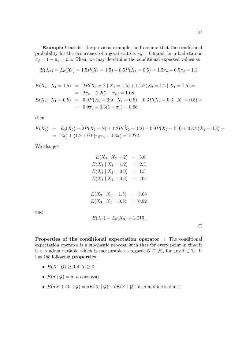
Example Consider the previous example, and assume that the conditionalprobability for the occurrence of a good state is πu = 0.6 and for a bad state isπd = 1 − πu = 0.4. Then, we may determine the conditional expected values as
E(X1) = E0(X1) = 1.5P (X1 = 1.5) + 0.5P (X1 = 0.5) = 1.5πu + 0.5πd = 1.1
E(X2 | X1 = 1.5) = 2P (X2 = 2 | X1 = 1.5) + 1.2P (X2 = 1.2 | X1 = 1.5) =
= 2πu + 1.2(1 − πu) = 1.68
E(X2 | X1 = 0.5) = 0.9P (X2 = 0.9 | X1 = 0.5) + 0.3P (X2 = 0.3 | X1 = 0.5) =
= 0.9πu + 0.3(1 − πu) = 0.66
then
E(X2) = E0(X2) = 2P (X2 = 2) + 1.2P (X2 = 1.2) + 0.9P (X2 = 0.9) + 0.3P (X2 = 0.3) =
= 2π2u + (1.2 + 0.9)πdπu + 0.3π2
d = 1.272.
We also get
E(X3 | X2 = 2) = 3.6
E(X3 | X2 = 1.2) = 2.3
E(X3 | X2 = 0.9) = 1.3
E(X3 | X2 = 0.3) = .35
E(X3 | X1 = 1.5) = 3.08
E(X3 | X1 = 0.5) = 0.92
andE(X3) = E0(X3) = 2.216.
Properties of the conditional expectation operator : The conditionalexpectation operator is a stochastic process, such that for every point in time itis a random variable which is measurable as regards G ⊆ Ft, for any t ∈ T. Ithas the following properties:
• E(X | G) ≥ 0 if X ≥ 0;
• E(a | G) = a, a constant;
• E(aX + bY | G) = aE(X | G) + bE(Y | G) for a and b constant;
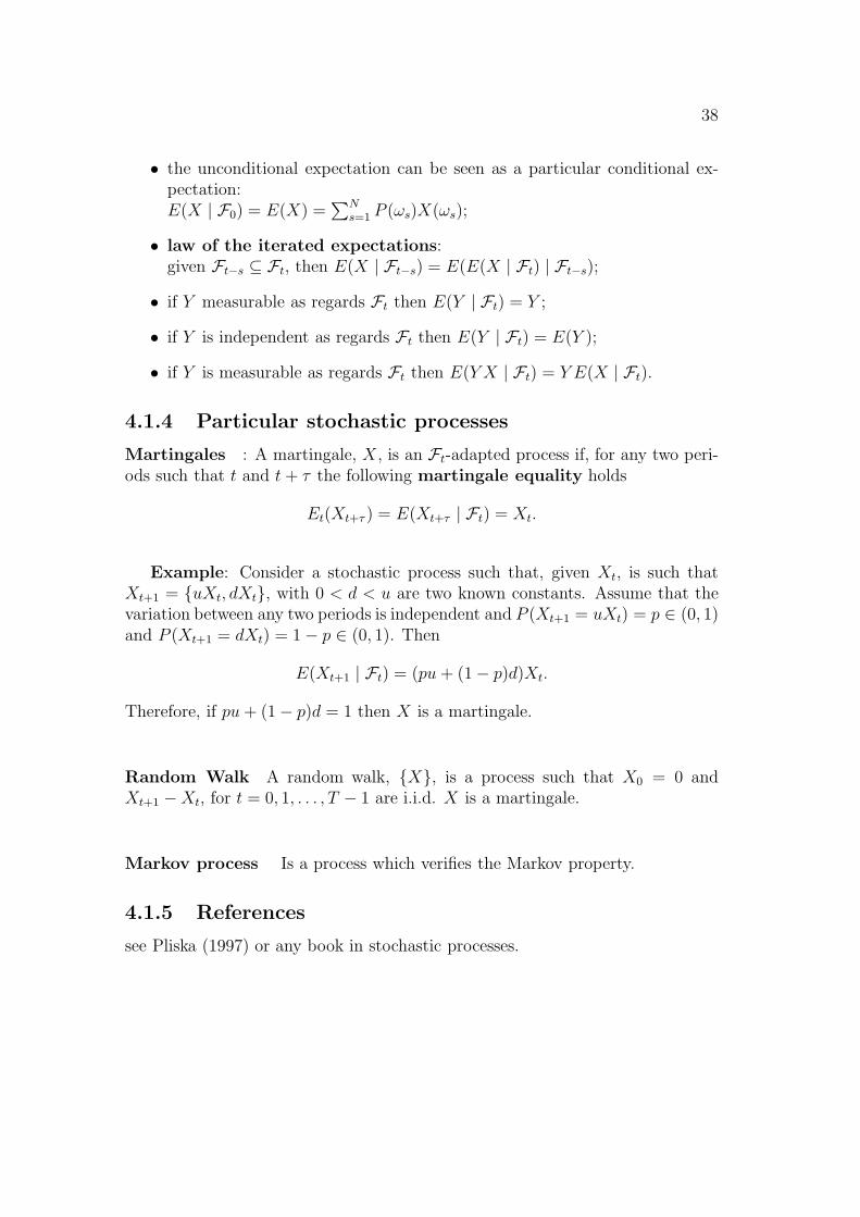
38
• the unconditional expectation can be seen as a particular conditional ex-pectation:E(X | F0) = E(X) =
∑Ns=1 P (ωs)X(ωs);
• law of the iterated expectations:given Ft−s ⊆ Ft, then E(X | Ft−s) = E(E(X | Ft) | Ft−s);
• if Y measurable as regards Ft then E(Y | Ft) = Y ;
• if Y is independent as regards Ft then E(Y | Ft) = E(Y );
• if Y is measurable as regards Ft then E(Y X | Ft) = Y E(X | Ft).
4.1.4 Particular stochastic processes
Martingales : A martingale, X, is an Ft-adapted process if, for any two peri-ods such that t and t + τ the following martingale equality holds
Et(Xt+τ ) = E(Xt+τ | Ft) = Xt.
Example: Consider a stochastic process such that, given Xt, is such thatXt+1 = uXt, dXt, with 0 < d < u are two known constants. Assume that thevariation between any two periods is independent and P (Xt+1 = uXt) = p ∈ (0, 1)and P (Xt+1 = dXt) = 1 − p ∈ (0, 1). Then
E(Xt+1 | Ft) = (pu + (1 − p)d)Xt.
Therefore, if pu + (1 − p)d = 1 then X is a martingale.
Random Walk A random walk, X, is a process such that X0 = 0 andXt+1 − Xt, for t = 0, 1, . . . , T − 1 are i.i.d. X is a martingale.
Markov process Is a process which verifies the Markov property.
4.1.5 References
see Pliska (1997) or any book in stochastic processes.

39
4.2 Stochastic Dynamic Programming
From the set of all feasible random sequences xt, utTt=0 where xt = xt(w
t) andut = ut(w
t) are Ft-adapted processes, choose a contingent plan x∗t , u
∗tT
t=0 suchthat
maxutT
t=0
E0
[T∑
t=0
βtf(ut, xt)
]
where
E0
[T∑
t=0
βtf(ut, xt)
]= E
[T∑
t=0
βtf(ut, xt) | F0
]
subject to the random sequence of constraints
x1 = g(x0, u0)
. . .
xt+1 = g(xt, ut, wt+1), t = 1, . . . , T − 2
. . .
xT = g(xT−1, uT−1, wT )
where x0 is given and wt is a Ft-adapted process representing the uncertaintyaffecting the agent decision.
Intuition: at the beginning of a period t xt and ut are known but the valueof xt+1, at the end of period t is conditional on the value of wt+1. The valuesof this random process may depend on an exogenous variable which is given bya stochastic process.
Let us call u∗tT
t=0 the optimal control. This is, in fact, a contingent plan,i.e., a planned sequence of decisions conditional on the sequence of states ofnature (or events).
At time t = 0 the optimal value of the state variable x0 is
V0 = V (x0) = E0
[T∑
t=0
βtf(u∗t , xt)
]=
= maxutT
t=0
E0
[T∑
t=0
βtf(ut, xt)
]=
= maxutT
t=0
E0
[f(u0, x0) + β
T∑t=1
βt−1f(u∗t , xt)
]=
= maxu0
f(u0, x0) + βE0
[maxutT
t=1
E1
[T∑
t=1
βt−1f(u∗t , xt)
]]
40
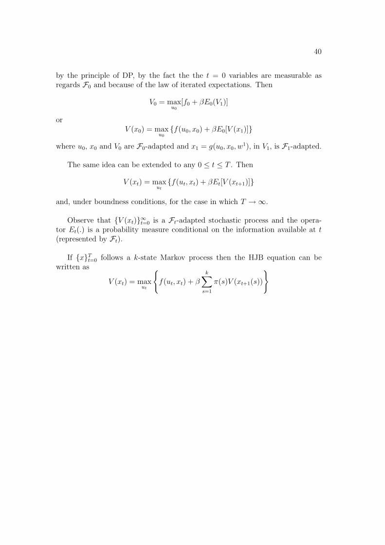
by the principle of DP, by the fact the the t = 0 variables are measurable asregards F0 and because of the law of iterated expectations. Then
V0 = maxu0
[f0 + βE0(V1)]
orV (x0) = max
u0
f(u0, x0) + βE0[V (x1)]
where u0, x0 and V0 are F0-adapted and x1 = g(u0, x0, w1), in V1, is F1-adapted.
The same idea can be extended to any 0 ≤ t ≤ T . Then
V (xt) = maxut
f(ut, xt) + βEt[V (xt+1)]
and, under boundness conditions, for the case in which T → ∞.
Observe that V (xt)∞t=0 is a Ft-adapted stochastic process and the opera-tor Et(.) is a probability measure conditional on the information available at t(represented by Ft).
If xTt=0 follows a k-state Markov process then the HJB equation can be
written as
V (xt) = maxut
f(ut, xt) + β
k∑s=1
π(s)V (xt+1(s))
41
4.3 Applications
4.3.1 The representative consumer
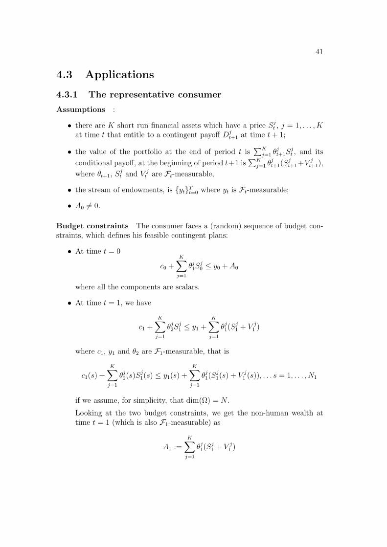
Assumptions :
• there are K short run financial assets which have a price Sjt , j = 1, . . . , K
at time t that entitle to a contingent payoff Djt+1 at time t + 1;
• the value of the portfolio at the end of period t is∑K
j=1 θjt+1S
jt , and its
conditional payoff, at the beginning of period t+1 is∑K
j=1 θjt+1(S
jt+1+V j
t+1),
where θt+1, Sjt and V j
t are Ft-measurable,
• the stream of endowments, is ytTt=0 where yt is Ft-measurable;
• A0 = 0.
Budget constraints The consumer faces a (random) sequence of budget con-straints, which defines his feasible contingent plans:
• At time t = 0
c0 +
K∑j=1
θj1S
j0 ≤ y0 + A0
where all the components are scalars.
• At time t = 1, we have
c1 +K∑
j=1
θj2S
j1 ≤ y1 +
K∑j=1
θj1(S
j1 + V j
1 )
where c1, y1 and θ2 are F1-measurable, that is
c1(s) +
K∑j=1
θj2(s)S
j1(s) ≤ y1(s) +
K∑j=1
θj1(S
j1(s) + V j
1 (s)), . . . s = 1, . . . , N1
if we assume, for simplicity, that dim(Ω) = N .
Looking at the two budget constraints, we get the non-human wealth attime t = 1 (which is also F1-measurable) as
A1 :=K∑
j=1
θj1(S
j1 + V j
1 )
42
Then, the sequence of instantaneous budget constraints is
yt + At ≥ ct +
K∑j=1
θjt+1S
jt , t ∈ [0,∞) (4.1)
At+1 =K∑
j=1
θjt+1
(Sj
t+1 + V jt+1
), t ∈ [0,∞) (4.2)
The representative consumer chooses a strategy of consumption, representedby the adapted process c := ct, t ∈ T and of financial transactions in Kfinancial assets, represented by the forecastable process θ := θt, t ∈ T, whereθt = (θ1
t , . . . , θKt ) in order to solve the following problem
maxc,θ
E0
[ ∞∑t=0
βtu(ct)
]
subject to equations (4.1)-(4.2), where A(0) = A0 is given and
limk→∞
Et
[βkSj
t+k
]= 0.
The last condition prevents consumers from playing Ponzi games. It rules outthe existence of arbitrage opportunities.
Solution by using dynamic programming
The HJB equation is
V (At) = maxct
u(ct) + βEt [V (At+1)] .
In our case, we may solve it by determining the optimal transactions strategy
V (At) = maxθjt+1,j=1,..,K
u
[yt + At −
K∑j=1
θjt+1S
jt
]+
+βEt
[V(At+1(θ
1t+1, . . . , θ
Kt+1))]
(4.3)
The optimality condition, is
−u′(ct)S
jt + βEt
[V
′(At+1)(S
jt+1 + V j
t+1)]
= 0,
for every asset j = 1, . . . , K.
43
In order to simplify this expression, we may apply the Benveniste-Scheinkmanformula (see (Ljungqvist and Sargent, 2000, p. 237) ) by substituting the opti-mality conditions in equation (4.3) and by diferentiating it in order to At. Thenwe get
V′(At) = u
′(ct).
However, we cannot go further without specifying the utility function, a particularprobability process and the stochastic processes for the asset prices and returns.
Intertemporal arbitrage condition
The optimality conditions may be rewritten as the following intertemporal arbi-trage conditions for the representative consumer
u′(ct)S
jt = βEt
[u
′(ct+1)(S
jt+1 + V j
t+1)], j = 1, . . . , K, t ∈ [0,∞). (4.4)
This model is imbedded in a financial market institutional framework that pre-vents the existence of arbitrage opportunities.
This imposes conditions on the asymptotic properties of prices, which imposesconditions on the solution of the consumer’s problem.
Taking equation (4.4) and operating recursively, the consumer chooses anoptimal trajectory of consumption such that (remember that the asset prices andthe payoffs are given to the consumer)
Sjt = Et
[ ∞∑τ=1
βτ u′(ct+τ )
u′(ct)V j
t+τ
], j = 1, . . . , K, t ∈ [0,∞) (4.5)
In order to prove this note that by repeatedly applying the law of iteratedexpectations
u′(ct)S
jt = βEt
[u
′(ct+1)(S
jt+1 + V j
t+1)]
=
= βEt
[u
′(ct+1)S
jt+1
]+ βEt
[u
′(ct+1)V
jt+1
]=
= βEt
βEt+1
[u
′(ct+2)(S
jt+2 + V j
t+2)]
+
+βEt
[u
′(ct+1)V
jt+1
]=
= βEt
βEt+1
[u
′(ct+2)S
jt+2
]+
+Et
βu
′(ct+1)V
jt+1 + β2Et+1
[u
′(c(t+2)V
jt+2
]=
= β2Et
[u
′(ct+2)S
jt+2
]+ Et
[2∑
τ=1
βτu′(ct+τ )V
jt+τ
]=
. . .

44
= βkEt
[u
′(ct+k)S
jt+k)
]+ Et
[k∑
τ=1
βτu′(ct+τ )V
jt+τ
]=
. . .
= limk→∞
βkEt
[u
′(ct+k)S
j(t + k)]
+ Et
[ ∞∑τ=1
βτu′(ct+τ )V
j(t + τ)
]
The condition for ruling out speculative bubbles,
limk→∞
βkEt
[u
′(ct+k)S
jt+k
]= 0
allows us to get equation (4.5).
Equity premium puzzle
If we define the return of asset j as
Rjt+1 =
Sjt+1 + V j
t+1
Sjt
the arbitrage relationship equation (4.4) becomes
mt = βEt
[mt+1R
jt+1
], j = 1, . . . , K, t ∈ [0,∞).
where mt ≡ u′(ct) This relation should hold for any asset, and, in particular for
riskless assets.Assume that there is an asset with certain return R0. Then mt = βEt
[mt+1R
0t+1
].
ThereforeβEt
[mt+1µ
jt+1
]= 0
where µjt = Rj
t − R0t the difference of the rates of return between the risky asset
j and the riskless asset.Then
covt(mt+1, µjt+1) + Et(mt+1)Et(µ
jt+1) = 0
ρ(mt+1, µjt+1) +
Et(mt+1)
σt(mt+1)
Et(µjt+1)
σt(µjt+1)
= 0
as | ρ(.) |≤ 1 then this imposes a restriction on the coefficient of variation ofthe marginal utility of consumption and the Sharpe index. As this should onlyverified in practice with a too large rate of risk aversion we have the equitypremium puzzle (see Mehra and Prescott (1985)).
References: Ljungqvist and Sargent (2000)

Chapter 5
Continuous time
5.1 Introduction to continuous time stochastic
processes
Assume that T = R+ and that the probability space is (Ω,F , P ) where Ω is ofinfinite dimension.
Let F = Ft, t ∈ T be a filtration over the probability space (Ω,F , P ).(Ω,F , F, P ) may be called a filtered probability space.
A stochastic process is a flow X = X(t, ω), t ∈ T, ω ∈ Ft.
5.1.1 Brownian motions
Definition 5. Brownian motion Assume the probability space (Ω,F , P x), asequence of sets Ft ∈ R and the stochastic process B = B(t), t ∈ T such that asequence of distributions over B(t) are given by
P x(B(t1) ∈ F1, . . . , B(tk) ∈ Fk) =
=
∫F1×...×Fk
p(t1, x, x1) . . . p(t2 − t1, x1, x2) . . . p(tk − tk−1, xk−1, xk)dx1dx2 . . . dxk,
where the conditional probabilities are
P (B(tj) = xj | B(ti) = xi) = p(tj − ti, xi, xj) = (2π(tj − ti))− 1
2 e− |xj−xi|2
2(tj−ti) .
Then B is a Brownian motion (or Wiener process), starting from the initial statex, where (P x(B(0) = x) = 1).
Remark We consider one-dimensional Brownian motions: that is, those forwhich the trajectories have continuous versions, B(ω) : T → R
n where t → Bt(ω),with n = 1.
45
46
Properties of B
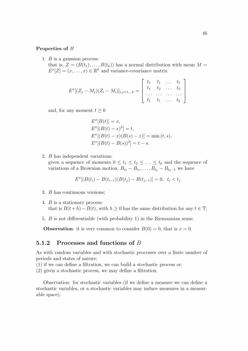
1. B is a gaussian process:that is, Z = (B(t1), . . . , B(tk)) has a normal distribution with mean M =Ex[Z] = (x, . . . , x) ∈ R
k and variance-covariance matrix
Ex[(Zj − Mj)(Zi − Mi)]i,j=1,...k =
t1 t1 . . . t1t1 t2 . . . t2. . . . . . . . . . . .t1 t1 . . . tk
and, for any moment t ≥ 0
Ex[B(t)] = x,
Ex[(B(t) − x)2] = t,
Ex[(B(t) − x)(B(s) − x)] = min (t, s),
Ex[(B(t) − B(s))2] = t − s.
2. B has independent variations:given a sequence of moments 0 ≤ t1 ≤ t2 ≤ . . . ≤ tk and the sequence ofvariations of a Brownian motion, Bt2 − Bt1 , . . . , Btk − Btk−1 we have
Ex[(B(ti) − B(ti−1)(B(tj) − B(tj−1)] = 0, ti < tj
3. B has continuous versions;
4. B is a stationary process:that is B(t+h)−B(t), with h ≥ 0 has the same distribution for any t ∈ T;
5. B is not differentiable (with probability 1) in the Riemannian sense.
Observation: it is very common to consider B(0) = 0, that is x = 0.
5.1.2 Processes and functions of B
As with random variables and with stochastic processes over a finite number ofperiods and states of nature:(1) if we can define a filtration, we can build a stochastic process or,(2) given a stochastic process, we may define a filtration.
Observation: for stochastic variables (if we define a measure we can define astochastic variables, or a stochastic variables may induce measures in a measur-able space).
47
Definition 6. (filtration)F = Ft, t ∈ T is a filtration if it verifies:(1) Fs ⊂ Ft if s < t(2) Ft ⊂ F for any t ∈ T
Definition 7. (Filtration over a Brownian motion)Consider a sequence of subsets of R, F1, F2, . . . , Fk where Fj ⊂ R and let B be aBrownian motion of dimension 1. Ft is a σ−algebra generated by B(s) such thats ≤ t, if it is the finest partition which contains the subsets of the form
ω : Bt1(ω) ∈ F1, . . . , Btk(ω) ∈ Fkse t1, t2, . . . , tk ≤ t.
Intuition Ft is the set of all the histories of Bj up to time t.
Definition 8. (Ft-measurable function)A function h(ω) is called a Ft-measurable if and only if it can be expressed as thelimit of the sum of function of the form
h(t, ω) = g1(B(t1))g2(B(t2)) . . . gk(B(tk)), tk ≤ t.
Definition 9. (Ft-adapted process)If F = Ft, t ∈ T is a filtration then the process g = g(t, ω), t ∈ T, ω ∈ Ω iscalled Ft-adapted if for every t ≥ 0 the function ω → gt(ω) is Ft-measurable.
For what is presented next, there are two important types of functions andprocesses:
Definition 10. (Class N functions)Let f : T × Ω → R. If
1. f(t, ω) is Ft-adapted;
2. E[∫ T
sf(t, ω)2dt
]< ∞,
then f ∈ N(s, T ), is called a class N(s, T ) function.
Definition 11. (Martingale)The stochastic process M = M(t), t ∈ T defined over (Ω,F , P ) is a martingaleas regards the filtration F if
1. M(t) is Ft-measurable, for any t ∈ T,

48
2. E[| M(t) |] < ∞, for any t ∈ T,
3. the martingale property holds
E[M(s) | Ft] = M(t),
for any s ≥ t.
One important property of the martingales is the Doob inequality: if M is amartingale and t → Mt(ω) is a continous version then for any p ≥ 1, T ≥ 0 andλ > 0, we have
P
[sup
0≤t≤T| M(t) |≥ λ
]≤ 1
λpE[| M(T ) |p].
5.1.3 Ito’s integral
Definition 12. (Ito’s integral)Let f be a function of class N and B(t) a one-dimensional Brownian motion.Then the Ito’s integral is denoted as
I(f, ω) =
∫ T
s
f(t, ω)dBt(ω)
If f is a class N function, it can be proved that the sequence of elementaryfunctions of class N φn where
∫ T
sφ(t, ω)dBt(ω) =
∑j≥0 ej(ω)[Btj+1
(ω)−Btj (ω)],
verifying limn→∞ E[∫ T
s| f − φn |2 dt] = 0, such that Ito’s integral is defined as
I(f, ω) =
∫ T
s
f(t, ω)dBt(ω) = limn→∞
∫ T
s
φn(t, ω)dBt(ω).
Intuition: as f is not differentiable (in the Riemannian sense), we may haveseveral definitions of integral. Ito’s integral approximates the function f by stepfunctions the ej evaluated at the beginning of the interval (tj+1, tj). TheStratonovich integral ∫ T
s
f(t, ω) dBt(ω)
evaluates in the intermediate point of the intervals.
Theorem 1. (Properties of Ito’s integral)Consider two class N function f, g ∈ N(0, T ), then
1.∫ T
sfdBt =
∫ U
sfdBt +
∫ T
UfdBt for almost every ω and for 0 ≤ s < U < T ;
2.∫ T
s(cf + g)dBt = c
∫ T
sfdBt +
∫ T
sgdBt for almost all ω and for c constant;

49
3. E(∫ T
sfdBt
)= 0;
4. has continuous versions up to time t, that is there is a stochastic process
J = J(t), t ∈ T such that P(J(t) =
∫ t
0fdBt
)= 1 for any 0 ≤ t ≤ T ;
5. Mt(ω) =∫ t
0f(s, ω)dBs is a martingale as regards the filtration Ft.
5.1.4 Stochastic integrals
Up to this point we presented a theory of integration, and implicitly of differen-tiation. The Ito’s presents a very useful stochastic counterpart of the chain ruleof differentiation.
Definition 13. (Ito’s process or stochastic integral)Let Bt be a one-dimensional Brownian motion over (Ω,F , P ). Let ν be a class
N function (i.e., such that P(∫ t
0ν(s, ω)2ds < ∞, ∀t ≥ 0
)= 1) and let µ be a
function of class Ht (i.e., such that
P(∫ t
0| µ(s, ω) | ds < ∞, ∀t ≥ 0
)= 1).
Then X = X(t), t ∈ T where X(t) has the domain (Ω,F , P ), is a stochastcintegral of dimension one if it is a stochastic process with the following equivalentrepresentations:
1. integral representation
X(t) = X(0) +
∫ t
0
µ(s, ω)ds +
∫ t
0
ν(s, ω)dBs
2. differential representation
dX(t) = u(t, ω)dt + ν(t, ω)dB(t)
Lemma 3. (Ito’s lemma)Let X(t) be a stochastic integral in its differential representation
dX(t) = µdt + νdB(t)
and let g(t, x) be a continuous differentiable function as regards its two arguments.Then
Y = Y (t) = g(t, X(t)), t ∈ Tis a stochastic process that verifies
dY (t) =∂g
∂t(t, X(t))dt +
∂g
∂x(t, X(t))dX(t) +
1
2
∂2g
∂x2(t, X(t))(dX(t))2.
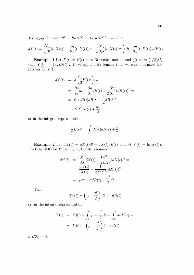
50
We apply the rule: dt2 = dtdB(t) = 0 e dB(t)2 = dt then
dY (t) =
(∂g
∂t(t, X(t)) +
∂g
∂x(t, X(t))µ +
1
2
∂2g
∂x2(t, X(t))ν2
)dt+
∂g
∂x(t, X(t))νdB(t).
Example 1 Let X(t) = B(t) be a Brownian motion and g(t, x) = (1/2)x2,then Y (t) = (1/2)B(t)2. If we apply Ito’s lemma then we can determine theprocess for Y (t)
dY (t) = d
(1
2B(t)2
)=
=∂g
∂tdt +
∂g
∂xdB(t) +
1
2
∂2g
∂x2(dB(t))2 =
= 0 + B(t)dB(t) +1
2dB(t)2
= B(t)dB(t) +dt
2,
or in the integral representation
1
2B(t)2 =
∫ t
0
B(s)dB(s) +t
2.
Example 2 Let dX(t) = µX(t)dt + σX(t)dB(t) and let Y (t) = ln(X(t)).Find the SDE for Y . Applying the Ito’s lemma
dY (t) =∂Y
∂XdX(t) +
1
2
∂2Y
∂X2(dX(t))2 =
=dX(t)
X(t)− 1
2X(t)2(dX(t))2 =
= µdt + σdB(t) − σ2
2dt
Then
dY (t) =
(µ − σ2
2
)dt + σdB(t)
or, in the integral representation
Y (t) = Y (0) +
∫ t
0
µ − σ2
2ds +
∫ t
0
σdB(s) =
= Y (0) +
(µ − σ2
2
)t + σB(t)
if B(0) = 0.

51
The process X is called a geometric Brownian motion, as its integral(which is the exp(Y ) is
X(t) = X(0)e
“µ−σ2
2
”t+σB(t)
.
Example 3: Let Y (t) = eaB(t). Find a stochastic integral for Y . From theIto’s lemma
dY (t) = aeaB(t)dB(t) +1
2a2eaB(t)(dB(t))2 =
=1
2a2eaB(t)dt + aeaB(t)dB(t)
the integral representation is
Y (t) = Y (0) +1
2a2
∫ t
0
eaB(s)ds + a
∫ t
0
eaB(s)dB(s)
5.1.5 Stochastic differential equations
Stochastic differential equations is a very vast field. Here we will only presentsome results that we will be useful afterwards.
Definition 14. (SDE)A stochastic differential equation can be defined as
dX(t)
dt= b(t, X(t)) + σ(t, X(t))W (t)
where b(t, x) ∈ R, σ ∈ R and W (t) represents a one-dimensional ”noise”.
Definition 15. (SDE: Ito’s interpretation)X(t) satisfies a stochastic differential equation is
dX(t) = b(t, X(t))dt + σ(t, X(t))dB(t)
or in the integral representation
X(t) = X(0) +
∫ t
0
b(s, X(s))ds +
∫ t
0
σ(s, X(s))dB(s).
How to solve, or study qualitatively, the solution of those equations ?
There are two solution concepts: weak and strong. We say that the processX is a strong solution if X(t) is Ft-adapted, and if B(t) is given, it verifies therepresentation of the SDE.

52
An important special case is the diffusion equation, which is the SDE withconstant coefficients and multiplicative noise
dX(t) = aX(t)dt + σX(t)dB(t).
As we already saw, the (strong) solution is the stochastic process X suchthat
X(t) = xe(a−σ2
2)t+σB(t)
where x is a random variable, which can be determined from x = X(0), whereX(0) is a given initial distribution , and B(t) =
∫ t
0dB(s), if B(0) = B0 = 0.
Properties:
1. asymptotic behavior:- if a − σ2
2< 0 then limt→∞ X(t) = 0 a.s.
- if a − σ2
2> 0 then limt→∞ X(t) = ∞ a.s.
- if a − σ2
2= 0 then limt→∞ X(t) will be finite a.s.
2. can we say anything about E[X(t)] ?
E(X(t)) = E(X(0))eat
To prove this, take Example 3 and observe that the stochastic integral ofY (t) = eaB(t) is
Y (t) = Y (0) +1
2a2
∫ t
0
eaB(s)ds + a
∫ t
0
eaB(s)dB(s)
taking expected values
E[Y (t)] = E[Y (0)] + E
[1
2a2
∫ t
0
eaB(s)ds
]+ aE
[∫ t
0
eaB(s)dB(s)
]=
= E[Y (0)] +1
2a2
∫ t
0
E[eaB(s)
]ds + 0
because eaB(s) is a f -class function (from the properties of the Brownian motian.Differentiating
dE[Y (t)]
dt=
1
2a2E[Y (t)]
as E[Y (0)] = 1. Then
E[Y (t)] = e12a2t
References: Oksendal (2003)
53
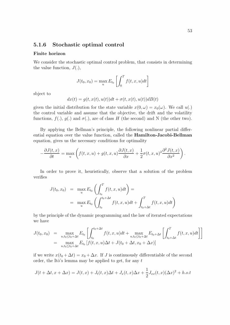
5.1.6 Stochastic optimal control
Finite horizon
We consider the stochastic optimal control problem, that consists in determiningthe value function, J(.),
J(t0, x0) = maxu
Et0
[∫ T
0
f(t, x, u)dt
]
sbject todx(t) = g(t, x(t), u(t))dt + σ(t, x(t), u(t))dB(t)
given the initial distribution for the state variable x(0, ω) = x0(ω). We call u(.)the control variable and assume that the objective, the drift and the volatilityfunctions, f(.), g(.) and σ(.), are of class H (the second) and N (the other two).
By applying the Bellman’s principle, the following nonlinear partial differ-ential equation over the value function, called the Hamilton-Jacobi-Bellmanequation, gives us the necessary conditions for optimality
−∂J(t, x)
∂t= max
u
(f(t, x, u) + g(t, x, u)
∂J(t, x)
∂x+
1
2σ(t, x, u)2∂2J(t, x)
∂x2
).
In order to prove it, heuristically, observe that a solution of the problemverifies
J(t0, x0) = maxu
Et0
(∫ T
t0
f(t, x, u)dt
)=
= maxu
Et0
(∫ t0+∆t
t0
f(t, x, u)dt +
∫ T
t0+∆t
f(t, x, u)dt
)
by the principle of the dynamic programming and the law of iterated expectationswe have
J(t0, x0) = maxu,t0≤t0+∆t
Et0
[∫ t0+∆t
t0
f(t, x, u)dt + maxu,t0≤t0+∆t
Et0+∆t
[∫ T
t0+∆t
f(t, x, u)dt
]]= max
u,t0≤t0+∆tEt0 [f(t, x, u)∆t + J(t0 + ∆t, x0 + ∆x)]
if we write x(t0 +∆t) = x0 +∆x. If J is continuously differentiable of the secondorder, the Ito’s lemma may be applied to get, for any t
J(t + ∆t, x + ∆x) = J(t, x) + Jt(t, x)∆t + Jx(t, x)∆x +1
2Jxx(t, x)(∆x)2 + h.o.t
54
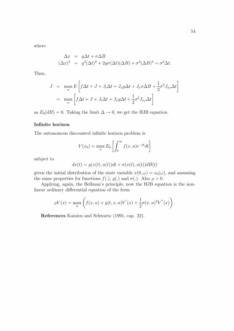
where
∆x = g∆t + σ∆B
(∆x)2 = g2(∆t)2 + 2gσ(∆t)(∆B) + σ2(∆B)2 = σ2∆t.
Then,
J = maxu
E
[f∆t + J + Jt∆t + Jxg∆t + Jxσ∆B +
1
2σ2Jxx∆t
]
= maxu
[f∆t + J + Jt∆t + Jxg∆t +
1
2σ2Jxx∆t
]
as E0(dB) = 0. Taking the limit ∆ → 0, we get the HJB equation.
Infinite horizon
The autonomous discounted infinite horizon problem is
V (x0) = maxu
E0
[∫ ∞
0
f(x, u)e−ρtdt
]
subject todx(t) = g(x(t), u(t))dt + σ(x(t), u(t))dB(t)
given the initial distribution of the state variable x(0, ω) = x0(ω), and assumingthe same properties for functions f(.), g(.) and σ(.). Also ρ > 0.
Applying, again, the Bellman’s principle, now the HJB equation is the non-linear ordinary differential equation of the form
ρV (x) = maxu
(f(x, u) + g(t, x, u)V
′(x) +
1
2σ(x, u)2V
′′(x)
).
References Kamien and Schwartz (1991, cap. 22).
55
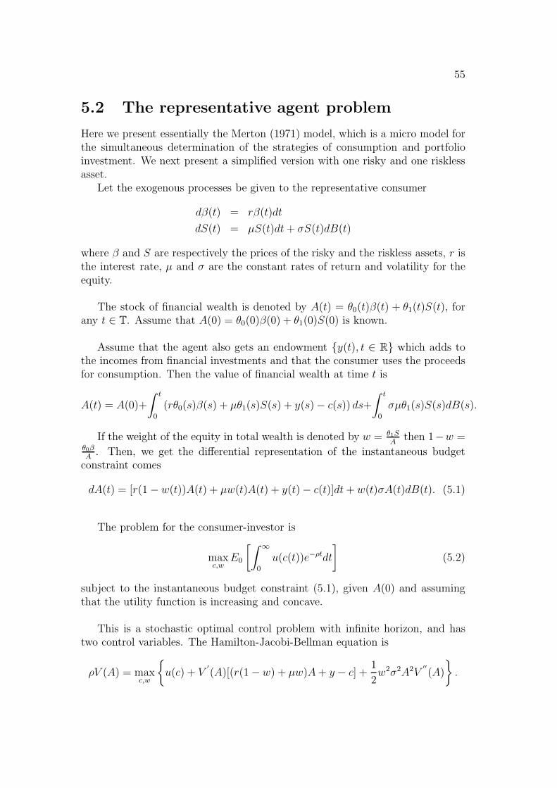
5.2 The representative agent problem
Here we present essentially the Merton (1971) model, which is a micro model forthe simultaneous determination of the strategies of consumption and portfolioinvestment. We next present a simplified version with one risky and one risklessasset.
Let the exogenous processes be given to the representative consumer
dβ(t) = rβ(t)dt
dS(t) = µS(t)dt + σS(t)dB(t)
where β and S are respectively the prices of the risky and the riskless assets, r isthe interest rate, µ and σ are the constant rates of return and volatility for theequity.
The stock of financial wealth is denoted by A(t) = θ0(t)β(t) + θ1(t)S(t), forany t ∈ T. Assume that A(0) = θ0(0)β(0) + θ1(0)S(0) is known.
Assume that the agent also gets an endowment y(t), t ∈ R which adds tothe incomes from financial investments and that the consumer uses the proceedsfor consumption. Then the value of financial wealth at time t is
A(t) = A(0)+
∫ t
0
(rθ0(s)β(s) + µθ1(s)S(s) + y(s) − c(s)) ds+
∫ t
0
σµθ1(s)S(s)dB(s).
If the weight of the equity in total wealth is denoted by w = θ1SA
then 1−w =θ0βA
. Then, we get the differential representation of the instantaneous budgetconstraint comes
dA(t) = [r(1 − w(t))A(t) + µw(t)A(t) + y(t) − c(t)]dt + w(t)σA(t)dB(t). (5.1)
The problem for the consumer-investor is
maxc,w
E0
[∫ ∞
0
u(c(t))e−ρtdt
](5.2)
subject to the instantaneous budget constraint (5.1), given A(0) and assumingthat the utility function is increasing and concave.
This is a stochastic optimal control problem with infinite horizon, and hastwo control variables. The Hamilton-Jacobi-Bellman equation is
ρV (A) = maxc,w
u(c) + V
′(A)[(r(1 − w) + µw)A + y − c] +
1
2w2σ2A2V
′′(A)
.

56
The first order necessary conditions allows us to get the optimal controls, i.e. theoptimal policies for consumption and portfolio composition
u′(c∗) = V
′(A), (5.3)
w∗ =(r − µ)V
′(A)
σ2AV ′′(A)(5.4)
If u′′(.) < 0 then the optimal policy function for consumption may be written as
c∗ = h(V′(A)). Plugging into the HJB equation, we get the differential equation
over V (A)
ρV (A) = u(h(V
′(A)‘)
)− h(V
′(A))V
′(A)(y + rA)V
′(A) − (r − µ)2(V
′(A))2
2σ2V ′′(A).
(5.5)In some cases the equation may be solve explicitly. In particular, let the utilityfunction be CRRA as
u(c) =c1−η − 1
1 − η, η > 0
and conjecture that the solution for equation (5.5) is of the type
V (A) = x(y + rA)1−η
for x an unknow constant. If it is indeed a solution, there should be a constant,dependent upon the parameters of the model, such that equation (5.5) holds.
First note that
V′(A) = (1 − η)rx(y + rA)−η
V′′(A) = −η(1 − η)r2x(y + rA)−η−1
then: the optimal consumption policy is
c∗ = (xr(1 − η))−1η (y + rA)
and the optimal portfolio composition is
w∗ =
(µ − r
σ2
)y + rA
ηrA
Interestingly it is a linear function of the ratio of total (human plus financialwealth y
r+ a ) over financial wealth.
After some algebra, we get
V (A) = Θ
(y + rA
r
)1−η

57
where 1
Θ ≡ 1
1 − η
[ρr(1 − η)
η− (1 − η)
2η2
(µ − r
σ
)2]−η
Then the optimal consumption is
c∗ =
(ρr(1 − η)
η− (1 − η)
2η2
(µ − r
σ
)2)(
y + rA
r
)
If we set the total wealth as W = yr
+ A, we may write the value function andthe policy functions for consumption and portfolio investment
V (W ) = ΘW 1−η
c∗(W ) = (1 − η)Θ− 1η W
w∗(W ) =
(µ − r
ησ2
)W
A.
Remark The value function follows a stochastic process which is a monotonousfunction for wealth. The optimal strategy for consumption follows a stochasticprocess which is a linear function of the process for wealth and the fraction ofthe risky asset in the optimal portfolio is a direct function of the premium of therisky asset relative to the riskless asset and is a inverse function of the volatility.
We see that the consumer cannot eliminate risk, in general. If we write
c∗ = χA, where χ ≡ (1 − η)Θ− 1η W
A, then the optimal process for wealth is
dA(t) = [r∗ + (µ − r)w∗ − χ]A(t)dt + σw∗A(t)dB(t)
where r∗ = rWA
, which is a linear SDE. Then as c∗ = c(A), if we apply the Ito’slemma we get
dc = χdA = c (µcdt + σcdB(t))
where
µc =r − ρ
η+
1 + η
2
(µ − r
ση
)2
σc =µ − r
ση.
The sde has the solution
c(t) = c(0) exp
(µc − σ2
c
2
)t + σcB(t)
, where µ−r
σis the Sharpe index, and the unconditional expected value for con-
sumption at time tE0[C(t)] = E0[C(0)]eµct.
References Merton (1971), Merton (1990)
1Of course, x = r−(1−η)Θ.

58
5.3 A stochastic continous time DGE for asset
prices
Now, we will consider a GE model in which the representative agent has thebehavior that we have just studied, but the where asset prices are determinedendogenously. We start with an economy in which there are only real forwardtransactions and then introduce a finance economy with complete markets. Theequivalence between the two economies allows for a simple determination of assetprices.
5.3.1 Arrow-Debreu equilbrium
Assumptions:
• information structure is given by the filtered probability space (Ω,F , F, P )where the filtration is F = F(t) : t ∈ R+. Associated to the filtration,there is a flow of unconditional probabilities P (t) : t ∈ R+ where π(t) =π(t, ω(t)) where ω(t) ∈ F(t), which are common knowledge. Consumptionand endowments c = c(t), t ∈ R and y = y(t), t ∈ R are adaptedprocesses to the filtration F, that is, c(t) and y(t) are Ft-measurable;
• the endowment follows the SDE
dy(t) = y(t)[µydt + σydB(t)] (5.6)
where, we assume for simplicity that the drift and the volatility coefficientsare constant and know. y(0) = y0 is also know and is deterministic;
• we assume that the consumers are homogeneous and have a von-NeumannMorgenstern utility function
V (c) = E0
[∫ ∞
0
u(c(t))e−ρtdt
], ρ > 0 (5.7)
where u′(.) > 0, u
′′(.) < 0 and u
′′′(.) > 0. We call, for any x > 0,
rr(x) ≡ −u′′(x)x
u′(x)(5.8)
πr(x) ≡ −u′′′(x)x
u′′(x)(5.9)
the coefficient of relative risk aversion and the coefficient of relativeprudence.
59
• there is a large (in fact infinite) number of contingent claim markets, op-erating at time t = 0, in which agents can contract for any future momentand state of nature, in which the price q(t, w(t)) is formed (with q(0) = 1)and qt is Ft-measurable. Therefore, agents face an instantaneous budgetconstraint, at time t = 0∫ ∞
0
∫Ft
(y(t, w)− c(t, w))dq(t, w(t))dt = 0
If we define dq(t, ω) = m(t, ω)dP (t, ω) then the budget constraint may beequivalently written as
E0
[∫ ∞
0
m(t)(y(t) − c(t))dt
]= 0 (5.10)
where m(0) = 1;
• there are some technical conditions over m, y and c which basically amountto the guarantee of boundedness: they should be class H functions)
Definition 16. The Arrow-Debreu equilibrium is defined by the Ft adapted pro-cesses c∗ = c∗(t), t ∈ R+ and m∗ = m∗(t), t ∈ R+ such that: (1) c∗ maximizesthe utility function (5.7) subject to the budget constraint (5.10); and (2) the equi-librium conditions hold
c(t, ω) = y(t, ω), ∀(t, ω) ∈ R+ × Ω
and the endowment process follows equation (5.6)
In order to determine it, we have to solve the consumers problem. Given theassumptions on boundedness we can form the Lagrangean
L = E0
[∫ ∞
0
(∫ ∞
0
u(c(t))e−ρt + λm(t)(y(t) − c(t))
)dt
]
where λ is a constant. The f.o.c are
u′(c(t, ω))e−ρt = λm(t, ω) (t, ω) ∈ R+ × Ω
As, at time t = 0 we have u′(c(0)) = λ then consumption is deterministic, and
we can writeu
′(c(t, ω))
u′(c(0))= eρtm(t, ω), (t, ω) ∈ R+ × Ω.
Therefore the equilibrium stochastic discount factor comes
m∗(t, ω) = e−ρt u′(y(t, ω))
u′(y(0)), (t, ω) ∈ R+ × Ω. (5.11)

60
is a stochastic process that depends on the endowment process m(t) = f(t, y(t)is Ft-measurable. If we use the Ito’s lemma we get
dm(t) = −m(t) (µm(y)dt + σm(y)dB(t)) (5.12)
where
µm = ρ + rr(y)
(µy − 1
2πr(y)σ2
y
)(5.13)
σm = rr(y)σy (5.14)
Exercise: prove this result.
For the case in which the utility function is CRRA as u(c) = c1−η−11−η
thecoefficients of relative risk aversion and relative prudence are
rr(y) = η, πr(y) = 1 + η
and then
µm = ρ + ηµy − 1
2η(1 + η)σ2
y , σm = ησy
Comments: the equilibrium stochastic discount factor is a linear SDE wherethe drift depends on the rate of time preference and on a linear function ofinstantaneous rate of growth and the variance of the endowment and the volatilitydepends only on the conditional standard deviation of the endowment. Therelative risk aversion affects the both the drift and the volatility and the relativeprudence affects the drift (i.e., it has first order effects).
5.3.2 Finance economy
Now assume that we have a finance economy, with the same structure as in section5.2.
Definition 17. (Radner) General equilibrium for a finance economy isdefined by the sequences of consumption c∗ = c∗(t), t ∈ R+, portfolio compo-sition w∗ = w∗(t), t ∈ R+ and asset prices S = S(t), t ∈ R+ such that theconsumer solves the problem given by equations (5.2)-(5.1) with rational expecta-tions over future asset prices and the markets clear.
In this section we will determine the equilibrium by proving its equivalencewith the Arrow-Debreu equlibrium.
For convenience, we rewrite the instantaneous budget constraint
dA(t) = [r(1 − w(t))A(t) + µw(t)A(t) + y(t) − c(t)]dt + w(t)σA(t)dB(t),
61
and assume that A(0) = 0 (analogously with the deterministic case).
Define the market price of risk as
x(t) ≡ µ(t) − r(t)
σ(t)
observe that now, µ(t), σ(t) and r(t) are endogenous; the first two are stochasticprocesses. Consider the process
dM(t) = −x(t)M(t)dB(t)
which is called in the literature the state density process. The process
M(t) = e−R t0 r(s)dsM(t)
is called the state density deflactor. Using the Ito’s lemma (prove this) it hasthe differential representation
dM(t) = −M (t) (r(t)dt + x(t)dB(t))
Now consider the deflated value of wealth defined as
Z(t) = M(t)A(t)
which is a Ft-measurable. By using the Ito’s lemma its differential representationis 2
dZ(t) = Z(t)[σ(t)w(t) − x(t)]dB(t) + M(t)(y(t) − c(t))dt
then
Z(T ) = Z(t) +
∫ T
t
M(s)(y(s) − c(s))ds +
∫ T
t
Z(s)[σ(s)w(s) − x(s)]dB(s)
Under certain conditions, a self-financing strategy holds, i.e,
Et[Z(T )] = Z(t) + Et
[∫ T
t
M(s)(y(s) − c(s))ds
]
If we set t = 0 and take T = ∞ and assume that there are no bubbles
E0[ limt→∞
M(t)A(t)] = 0
2Exercise: prove this result by using the following version of the It0’s lemma: for y =f(x1, x2)
dy =∂f
∂x1dx1 +
∂f
∂x2dx2 +
12
∂2f
∂x21
(dx1)2 +12
∂2f
∂x22
(dx2)2 +∂2f
∂x1∂x2dx1dx2.
62
then we get the intertemporal budget constraint as
E0
[∫ ∞
0
M(s)(y(s)− c(s))ds
]= 0
which is formally identical to the restriction for the consumer problem in theArrow-Debreu economy. This means that the state price deflactor M = m.
Therefore:
r(t) = µm(t) (5.15)
µ(t) − r(t)
σ(t)= σm(t) (5.16)
gives the endogenous instantaneous risk premium.References: Duffie (1996) (Cvitanic and Zapatero, 2004, p. 395-398)
5.4 Stochastic Ramsey model
Let us assume that the economy is represented by the equations
dK(t) = F (K(t), L(t)) − C(t)
dL(t) = µL(t)dt + σLdB(t)
where we assume that F (K, L) is linearly homogeneous, given the (deterministic)initial stock of capital and labor K(0) = K0 and L(0) = L0.
The growth of the labor input (or its productivity) is stochastic.Let us define the variables in intensity terms
k(t) ≡ K(t)
L(t), c(t) ≡ C(t)
L(t)
We can get the restriction of the economy as a single equation on k by using theIto’s lemma
dk =∂k
∂KdK +
∂k
∂LdL +
1
2
∂2k
∂K2(dK)2 +
1
2
∂2k
∂K∂LdKdL +
1
2
∂2k
∂L2(dL)2
=F (K, L) − C
Ldt − K(µLdt + σLdB(t))
L2+ σ2 K
Ldt
=(f(k) − c − (µ − σ2)k
)dt − σ2kdB(t)
if we set f(k) = F(
KL, 1).
The HJB equation is
ρV (k) = maxc
u(c) + V′(k)(f(k) − c − (µ − σ2)k
)+
1
2(kσ)2V ”(k)

63
the optimality condition is again
u′(c) = V
′(k)
and, we get again a 2nd order ODE
ρV (k) = u(h(k)) + V′(k)(f(k) − h(k) − (µ − σ2)k
)+
1
2(kσ)2V ”(k).
Again, we assume the benchmark particular case: u(c) = c1−θ
1−θand f(k) =
kα. Then the optimal policy function becomes
c∗ = V′(k)−
1σ
and the HJB becomes
ρV (k) =θ
1 − θV
′(k)
θ−1θ + V
′(k)(kα −−(µ − σ2)k
)+
1
2(kσ)2V ”(k)
We can get, again, a closed form solution if we particulare further: θ = α.Again we conjecture that the solution if of the form
V (k) = B0 + B1kα
Using the same methods as before we get
B0 = (1 − α)B1
ρ
B1 =1
1 − α
[(1 − α)θ
(1 − θ)(ρ − (1 − α)2σ2)
]α
.
Then
V (k) = B1
(1 − α
ρ+ k1−α
)and
c∗ = c(k) =
((1 − θ)(ρ − (1 − α)2σ2)
(1 − α)θ
)k ≡ k
as we see an increase in volatility decreases consumption for every level of thecapital stock.
Then the optimal dynamics of the per capita capital stock is the SDE
dk∗(t) =(f(k∗(t)) − (µ + − σ2)k∗(t)
)dt − σ2k∗(t)dB(t).
In this case we can not solve it explicitly as in the deterministic case.References: Merton (1975), Merton (1990)
Bibliography
Richard Bellman. Dynamic Programming. Princeton University Press, 1957.
L. M. Benveniste and J. A. Scheinkman. On the differentiability of the valuefunction in dynamic models of economics. Econometrica, 47(3):3, May 1979.
Dimitri P. Bertsekas. Dynamic Programming and Stochastic Control. AcademicPress, 1976.
William A. Brock and Leonard Mirman. Optimal economic growth and uncer-tainty: the discounted case. Journal of Economic Theory, 4:479–513, 1972.
Jaksa Cvitanic and Fernando Zapatero. Introduction to the Economics and Math-ematics of Financial Markets. MIT Press, 2004.
Darrell Duffie. Dynamic Asset Pricing Theory, 2nd ed. Princeton, 1996.
Wendell H. Fleming and Raymond W. Rishel. Deterministic and Stochastic Op-timal Control. Springer-Verlag, 1975.
Morton I. Kamien and Nancy L. Schwartz. Dynamic optimization, 2nd ed. North-Holland, 1991.
Lars Ljungqvist and Thomas J. Sargent. Recursive Macroeconomic Theory. MITPress, 2000.
Rajnish Mehra and Edward C. Prescott. The equity premium: a puzzle. Journalof Monetary Economics, 15:145–162, 1985.
Robert Merton. Optimum consumption and portfolio rules in a continuous timemodel. Journal of Economic Theory, 3:373–413, 1971.
Robert Merton. An Asymptotic Theory of Growth under Uncertainty. Review ofEconomic Studies, 42:375–93, July 1975.
Robert Merton. Continuous Time Finance. Blackwell, 1990.
Bernt Oksendal. Stochastic Differential Equations. Springer, 6th edition, 2003.
64

65
S. Pliska. Introduction to Mathematical Finance. Blackwell, 1997.
Thomas J. Sargent. Dynamic Macroeconomic Theory. Harvard University Press,Cambridge and London, 1987.
Nancy Stokey and Robert Lucas. Recursive Methods in Economic Dynamics.Harvard University Press, 1989.