introduction to decision analysis - ulisboa · 5/11/2016 1 introduction to decision analysis...
TRANSCRIPT

5/11/2016
1
INTRODUCTION TO DECISION ANALYSIS
Introduction
� Decision often must be made in uncertain
environments.
� Examples:
� Manufacturer introducing a new product in the
marketplace.
� Government contractor bidding on a new contract.
� Oil company deciding to drill for oil in a particular
location.
� Type of decisions that decision analysis is designed to
address.
� Making decisions with or without experimentation.
608

5/11/2016
2
Prototype example
� Goferbroke Company owns a tract of land that can
contain oil.
� Contracted geologist reports that chance of oil is 1 in 4.
� Another oil company offers 90 000€ for land.
� Cost of drilling is 100 000€. If oil is found, revenue is
800 000€ (expected profit is 700 000€).
609
Status of land Status of land Status of land Status of land
AlternativeAlternativeAlternativeAlternative
PayoffPayoffPayoffPayoff
Oil Oil Oil Oil DryDryDryDry
Drill for oil 700 000€ –100 000€
Sell the land 90 000€ 90 000€
Chance of status 1 in 4 3 in 4
Decision making without experimentation
� Analogy to game theory:
� Players: decision maker (player 1) and nature (player 2).
� Available strategies for 2 players: alternative actions
and possible states of nature, respectively.
� Combination of strategies results in some payoff to
player 1 (decision maker).
� But, are both players rational?
610

5/11/2016
3
Decision making without experimentation
� The decision maker needs to choose one of the
alternative actions.
� Nature choose one of the possible states of nature.
� Each combination of an action and state of nature
results in a payoff, which is one entry of a payoff table.
� Probabilities for states of nature provided by the prior
distribution are prior probabilities.
� Payoff table is used to find an optimal action for the
decision making according to an appropriate criterion.
611
Payoff table for Goferbroke Co. problem
612
AlternativeAlternativeAlternativeAlternative
State of natureState of natureState of natureState of nature
Oil Oil Oil Oil DryDryDryDry
1. Drill for oil 700 –100
2. Sell the land 90 90
Prior probability 0.25 0.75

5/11/2016
4
Maximin payoff criterion
� Game against nature.
� Maximin payoff criterion: For each possible decision
alternative, find the minimum payoff over all states.
Next, find the maximum of these minimum payoffs.
� Best guarantee of payoff: pessimistic viewpoint.
613
AlternativeAlternativeAlternativeAlternative
State of natureState of natureState of natureState of nature
Oil Oil Oil Oil DryDryDryDry Minimum Minimum Minimum Minimum
1. Drill for oil 700 –100 –100
2. Sell the land 90 90 90909090 ←←←← MaximinMaximinMaximinMaximin valuevaluevaluevalue
Prior probability 0.25 0.75
Maximum likelihood criterion
� Maximum likelihood criterion: Identify most likely
state. For this state, find decision alternative with the
maximum payoff. Choose this action.
� Most likely state: ignores important information and
low-probability big payoff.
614
AlternativeAlternativeAlternativeAlternative
State of natureState of natureState of natureState of nature
Oil Oil Oil Oil DryDryDryDry
1. Drill for oil 700 –100
2. Sell the land 90 90909090 ←←←← Maximum in this columnMaximum in this columnMaximum in this columnMaximum in this column
Prior probability 0.25 0.75
↑↑↑↑Most likelyMost likelyMost likelyMost likely

5/11/2016
5
Bayes’ decision rule
� Bayes’ decision rule: Using prior probabilities,
calculate the expected value of payoff for each
decision alternative. Choose the action with the
maximum expected payoff.
� For the prototype example:
� E[Payoff (drill)] = 0.25(700) + 0.75(–100) = 100.
� E[Payoff (sell)] = 0.25(90) + 0.75(90) = 90.
� Incorporates all available information (payoffs and
prior probabilities).
� What happens when probabilities are inaccurate?
615
Sensitivity analysis with Bayes’ rules
� Prior probabilities can be questionable.
� True probabilities of having oil are 0.15 to 0.35 (so,
probabilities for dry land are from 0.65 to 0.85).
� p = prior probability of oil.
� Example: expected payoff from drilling for any p:
� E[Payoff (drill)] = 700p – 100(1 – p) = 800p – 100.
� In figure, the crossover point is where the decision
changes from one alternative to another:
� E[Payoff (drill)] = E[Payoff (sell)]
� 800p – 100 = 90 → p = 0.2375
616

5/11/2016
6
Expected payoff for alternative changes
617
The decision is very
sensitive to p!
Decision making with experimentation
� Improved estimates are called posterior probabilities.
� Example: a detailed seismic survey costs 30 000€.
� USS: unfavorable seismic soundings: oil is fairly unlikely.
� FSS: favorable seismic soundings: oil is fairly likely.
� Based on past experience, the following probabilities
are given:
� P(USS| State=Oil) = 0.4; P(FSS| State=Oil) = 1 – 0.4 = 0.6
� P(USS| State=Dry) = 0.8; P(FSS| State=Dry) = 1 – 0.8 = 0.2
618

5/11/2016
7
Posterior probabilities
� n = number of possible states.
� P(State = state i) = prior probability that true state is
state i.
� Finding = finding from experimentation (random var.)
� Finding j = one possible value of finding.
� P(State = state i | Finding = finding j) = posterior
probability that true state of nature is state i, given
Finding = finding j.
� Given P(State=state i) and P(Finding=find j|State=state i),
what is P(State=state i | Finding = finding j)?
619
Posterior probabilities
� From probability theory the Bayes’ theorem can be
obtained:
620
1
(State = state | Finding = finding )
(Finding = finding |State = state ) (State = state )
(Finding = finding |State = state ) (State = state )n
k
P i j
P j i P i
P j k P k=
=
=
∑

5/11/2016
8
Bayes’ theorem in prototype example
� If seismic survey in unfavorable (USS):
� If seismic survey in favorable (FSS):
621
0.4(0.25) 1(State = Oil | Finding = USS) ,
0.4(0.25) 0.8(0.75) 7P = =
+
1 6(State = Dry | Finding = USS) 1 .
7 7P = − =
0.6(0.25) 1(State = Oil | Finding = FSS) ,
0.6(0.25) 0.2(0.75) 2P = =
+
1 1(State = Dry | Finding = FSS) 1 .
2 2P = − =
Probability tree diagram
622

5/11/2016
9
Expected payoffs
� Expected payoffs can be found using again Bayes’
decision rule for the prototype example, with posterior
probabilities replacing prior probabilities:
� Expected payoffs if finding is USS:
� Expected payoffs if finding is FSS:
623
1 6[Payoff (drill | Finding = USS) (700) ( 100) 30 15.7
7 7E = + − − = −
1 6[Payoff (sell | Finding = USS) (90) (90) 30 60
7 7E = + − =
1 1[Payoff (drill | Finding = FSS) (700) ( 100) 30 270
2 2E = + − − =
1 1[Payoff (sell | Finding = FSS) (90) (90) 30 60
2 2E = + − =
Optimal policy
� Using Bayes’ decision rule, the optimal policy of
optimizing payoff is given by:
� Is it worth spending 30.000€ to conduct the
experimentation?
624
Finding from Finding from Finding from Finding from
seismic surveyseismic surveyseismic surveyseismic survey
Optimal Optimal Optimal Optimal
alternativealternativealternativealternative
Expected payoff Expected payoff Expected payoff Expected payoff
excluding cost of surveyexcluding cost of surveyexcluding cost of surveyexcluding cost of survey
Expected payoff Expected payoff Expected payoff Expected payoff
including cost of surveyincluding cost of surveyincluding cost of surveyincluding cost of survey
USS Sell the land 90 60
FSS Drill for oil 300 270

5/11/2016
10
Value of experimentation
� Before performing an experimentation, determine its
potential value.
� Two methods:
1. Expected value of perfect information – it is assumed
that all uncertainty is removed. Provides an upper
bound of potential value of experiment.
2. Expected value of information – is the expected
increase in payoff, not just its upper bound.
625
Expected value of perfect information
� Expected value of perfect information (EVPI) is:
EVPI = expected payoff with perfect information – expected payoff
without experimentation
� Example: EVPI= 242.5–100 = 142.5. This value is > 30
626
State of natureState of natureState of natureState of nature
AlternativeAlternativeAlternativeAlternative OilOilOilOil DryDryDryDry
1. Drill for oil 700 –100
2. Sell the land 90 90
Maximum payoff 700 90
Prior probability 0.25 0.75
Expected payoff with perfect information = 0.25(700) + 0.75(90) = 242.5

5/11/2016
11
Expected value of information
� Requires expected payoff with experimentation:
� Example: see probability tree diagram, where:
P(USS) = 0.7, P(FSS) = 0.3.
� Expected payoff (excluding cost of survey) was
obtained in optimal policy:
� E(Payoff| Finding = USS) = 90,
� E(Payoff| Finding = FSS) = 300.
627
Expected payoff with experimentation
(Finding = finding ) [payoff | Finding = finding ]j
P j E j
=
∑
Expected value of information
� So, expected payoff with experimentation is
� Expected payoff with experim. = 0.7(90) + 0.3(300) = 153.
� Expected value of experimentation (EVE) is:
EVE = expected payoff with experimentation –
expected payoff without experimentation
� Example: EVE = 153 – 100 = 53.
� As 53 exceeds 30, the seismic survey should be done.
628

5/11/2016
12
Decision trees
� Prototype example has a sequence of two questions:
1. Should a seismic survey be conducted before an
action is chosen?
2. Which action (drill for oil or sell the land) should be
chosen?
� These questions have a corresponding decision tree.
� Junction points are nodes, and lines are branches.
� A decision node, represented by a square, indicates
that a decision needs to be made at that point.
� An event node, represented by a circle, indicates that
a random event occurs at that point.
629
Decision tree for prototype example
630

5/11/2016
13
Decision tree with probabilities
631
cash flow
probability
Performing the analysis
1. Start at right side of decision tree and move one
column at a time. For each column, perform step 2 or
step 3, depending if nodes are event or decision nodes.
2. For each event node, calculate its expected payoff, by
multiplying expected payoff of each branch by
probability of that branch and summing these
products.
3. For each decision node, compare the expected payoffs
of its branches, and choose alternative with largest
expected payoff. Record the choice by inserting a
double dash in each rejected branch.
632

5/11/2016
14
Decision tree with analysis
633
Optimal policy for prototype example
� The decision tree results in the following decisions:
1. Do the seismic survey.
2. If the result is unfavorable, sell the land.
3. If the result is favorable, drill for oil.
4. The expected payoff (including the cost of the seismic
survey) is 123 (123 000€).
� Same result as obtained with experimentation.
� For any decision tree, the backward induction
procedure always will lead to the optimal policy.
634
5/11/2016
15
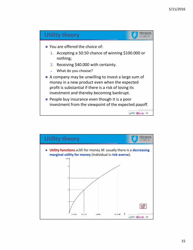
Utility theory
� You are offered the choice of:
1. Accepting a 50:50 chance of winning $100.000 or
nothing;
2. Receiving $40.000 with certainty.
� What do you choose?
� A company may be unwilling to invest a large sum of
money in a new product even when the expected
profit is substantial if there is a risk of losing its
investment and thereby becoming bankrupt.
� People buy insurance even though it is a poor
investment from the viewpoint of the expected payoff.
635
Utility theory
� Utility functions u(M) for money M: usually there is a decreasing
marginal utility for money (individual is risk-averse).
636

5/11/2016
16
Utility function for money
� It is also possible to exhibit a mixture of these kinds of
behavior (risk-averse, risk seeker, risk-neutral)
� An individual’s attitude toward risk may be different
when dealing with one’s personal finances than when
making decisions on behalf of an organization.
� When a utility function for money is incorporated into
a decision analysis approach to a problem, this utility
function must be constructed to fit the preferences
and values of the decision maker involved. (The
decision maker can be either a single individual or a
group of people.)
637
Utility theory
� Fundamental property: the decision maker’s utility
function for money has the property that the decision
maker is indifferent between two alternatives if they
have the same expected utility.
� Example. Offer: an opportunity to obtain either
$100000 (utility = 4) with probability p or nothing
(utility = 0) with probability 1 – p. Thus, E(utility) = 4p.
� Decision maker is indifferent for e.g.:
� Offer with p = 0.25 (E(utility) = 1) or definitely
obtaining $10 000 (utility = 1).
� Offer with p = 0.75 (E(utility) = 3) or definitely
obtaining $60 000 (utility = 3).
638

5/11/2016
17
Role of utility theory
� If utility function is used to measure worth of possible
monetary outcomes, Bayes’ decision rule replaces
monetary payoffs by corresponding utilities.
� Thus, optimal action is the one that maximizes the
expected utility.
� Note that utility functions my not be monetary.
� Example: doctor’s decision alternatives in treating a
patient involves the future health of the patient.
639
Applying utility theory to example
� The Goferbroke Co. does not have much capital, so a
loss of 100 000€ would be quite serious.
� The complete utility function can be found using the
following values:
640
Monetary payoffMonetary payoffMonetary payoffMonetary payoff UtilityUtilityUtilityUtility
–130 –150
–100 –105
60 60
90 90
670 580
700 600

5/11/2016
18
Utility function for Goferbroke Co.
641
Estimating u(M)
� A popular form is the exponential utility function:
� R = decision maker’s risk tolerance.
� This is designing a risk-averse individual.
� For prototype example, R = 2250 for u(670), and
R = 465 for u(–130).
� Note that, in general, it is not possible to have
different values of R.
642
( ) 1M
Ru M R e−
= −

5/11/2016
19
Decision trees with utility function
� The solution is exactly the same as before, except for
substituting utilities for monetary payoffs.
� Thus, the value obtained to evaluate each fork of the
tree is now the expected utility rather than the
expected monetary payoff.
� Optimal decisions selected by Bayes’ decision rule
maximize the expected utility for the overall problem.
643
Decision tree using utility function
644
Different decision tree
but same optimal policy.