introduction to data mining -...

Introduction to Data Mining

• People have been seeking patterns in data since human life began: hunters seek patterns in animal

migration behavior, farmers seek patterns in crop growth, politicians seek patterns in voter opinion and

lovers seek patterns in their partners’ responses...

• But we are overwhelmed with data. The amount of data in our lives seems to increase dramatically. As

the volume of data increases, inexorably, the proportion of it that people understand decreases.

• Lying hidden in all this data is information, potentially useful information that is rarely made explicit or

taken advantage of.

1

• A scientist’s job is to make sense of data, to discover the patterns that govern how the physical world

works and encapsulate them in theories that can be used for predicting what will happen in new situa-

tions.

• A tentative definition of Data Mining: Advanced methods for exploring and modeling relationships in

large amounts of data.

• There are other similar definitions. However, the term exploring and modeling relationships in data has

a much longer history than the term data mining.

• Data mining analysis has been limited by the computing power. For example, the computer IBM 7090

was a transistorized machine introduced in 1959. It had a processor speed of approximately 0.5 MHz

and roughly 0.2 MB of RAM using ferrite magnetic cores.

2

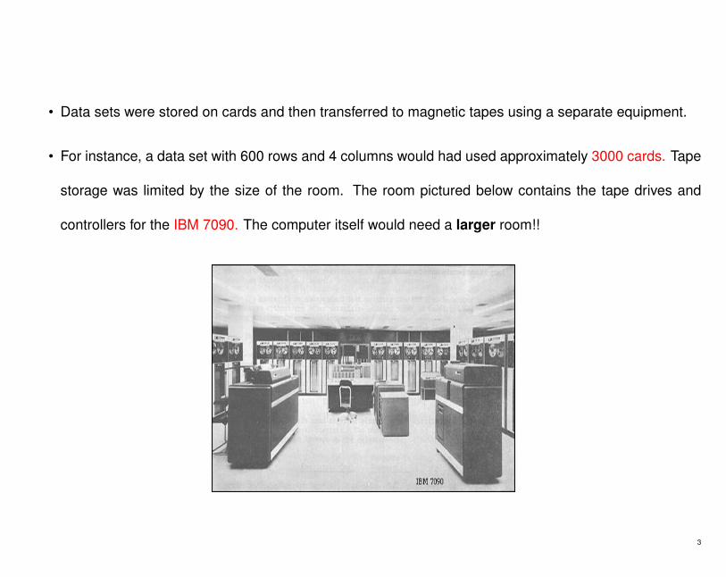
• Data sets were stored on cards and then transferred to magnetic tapes using a separate equipment.

• For instance, a data set with 600 rows and 4 columns would had used approximately 3000 cards. Tape

storage was limited by the size of the room. The room pictured below contains the tape drives and

controllers for the IBM 7090. The computer itself would need a larger room!!

3

• In data mining, data are stored electronically and searchings are automated by computers.

• Computer performance has been doubling every 24 months. This has led to technological advances in

storage structures and a corresponding increase in MB of storage space per dollar.

• The Parkinson’s law of data: Data expands to fill the space available for storage.

• The amount of data in the world has been doubling every 18 to 24 months. Multi-gigabyte commercial

databases are now commonplace.

• Economists, statisticians, forecasters, and communication engineers have long worked with the idea

that patterns in data can be sought automatically, identified, validated, and used for prediction...

4

• Historically, most data were generated or collected for research purposes. But, today, big compa-

nies have massive amounts of operational data which were not generated for data analysis in mind.

It is aptly characterized as opportunistic. This is in contrast to experimental data where factors are

controlled and varied in order to answer specific questions.

• The owners of the data and sponsors of the analyses are typically not researchers. The objectives are

usually to support business decisions.

• Database marketing makes use of customer and transaction databases to improve product introduc-

tion, cross-sell, trade-up, and customer loyalty promotions.

• One of the facets of customer relationship management is concerned with identifying and profiling

customers who are likely to switch brands or cancel services (churn). These customers can then be

targeted for loyalty promotions.

5

• EXAMPLE: Credit scoring is chiefly concerned with whether to extend credit to an applicant. The aim is

to anticipate and reduce defaults and serious delinquencies. Other credit risk management concerns

are the maintenance of existing credit lines (should the credit limit be raised?) and determining the best

action to be taken on delinquent accounts.

• The aim of fraud detection is to uncover the patterns that characterize deliberate deception. These

patterns are used by banks to prevent fraudulent credit card transactions and bad checks, by telecom-

munication companies to prevent fraudulent calling card transactions, and by insurance companies to

identify fictitious or abusive claims.

• EXAMPLE: Healthcare informatics is concerned with decision-support systems that relate clinical infor-

mation to patient outcomes. Practitioners and healthcare administrators use the information to improve

the quality and cost effectiveness of different therapies and practices.

6

DEFINITIONS I

• The analytical tools used in data mining were developed mainly by statisticians, artificial intelligence

(AI) researchers, and database system researchers.

• One consequence of the multidisciplinary flavor of data mining methods is a confusing terminology.

The same terms are often used in different senses and contexts and synonyms abound.

• KDD (knowledge discovery in databases) is a multidisciplinary research area concerned with the ex-

traction of patterns from large databases. It is sometimes used synonymously with data mining.

• Machine learning is concerned with creating and understanding semiautomatic learning methods.

• Pattern recognition has its roots in engineering and is typically concerned with image classification.

• Neurocomputing is, itself, a multidisciplinary field concerned with neural networks.

7

• Many people think data mining means magically discovering hidden nuggets of information without

having to formulate the problem and without regard to the structure or content of the data. But, this is

an unfortunate misconception.

• The database community has a tendency to view data mining methods as only more complicated types

of database queries.

• For example, standard query tools can answer questions such as how many surgeries, resulted in

hospital, stays longer than 10 days?

But data mining is needed for more complicated queries such as which are the most important predic-

tors of an excessive length of stay?

• The problem translation step involves determining what analytical methods are relevant to the objec-

tives.

9

DEFINITIONS II

• Predictive modeling or supervised prediction or supervised learning is the fundamental data mining

task. The training data set consists of cases or observations, examples, instances or records.

• Associated with each case is a vector of input variables (or predictors, features, explanatory variables,

independent variables) and a target variable (or response, outcome, dependent variable). The training

data is used to construct a model (rule) that can predict the values of the target from the inputs.

• The task is referred to as supervised because the prediction model is constructed from data where the

target is known. It allows you to predict new cases when the target is unknown. Typically, the target is

unknown because it refers to a future event.

• The inputs may be numeric variables such as income. They may be nominal variables such as occu-

pation. They are often binary variables such as home ownership.

10

• The main differences among analytical methods for predictive modeling depend on the type of target

variable.

• In Supervised Classification, the target is a class label (categorical). The training data consist of

labeled cases. The aim is to construct a model (classifier ) that can allocate cases to the classes using

only the values of the inputs.

• For example, Regression Analysis is supervised prediction technique where the target is a continuous

variable, although it can also be used more generally; for example in logistic regression. The aim is to

construct a model that can predict the values of the target from some inputs.

• In Survival Analysis, the target is the time until some event occurs. The outcome for some cases may

be censored : all that is known is that the event has not yet occurred.

12

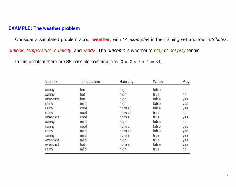
EXAMPLE: The weather problem

Consider a simulated problem about weather, with 14 examples in the training set and four attributes:

outlook , temperature, humidity , and windy . The outcome is whether to play or not play tennis.

In this problem there are 36 possible combinations (3× 3× 2× 2 = 36).

13

A set of rules, learned from this information, might look as follows:

If outlook=sunny and humidity=high then play=no

If outlook=rainy and windy=true then play=no

If outlook=overcast then play=yes

If humidity=normal then play=yes

If none of the above then play=yes

• But these rules have to be interpreted in order.

• A set of rules that are intended to be interpreted in sequence is called a decision list .

• The rules, interpreted as a decision list, classify correctly all of the examples in the table whereas

taken individually (out of context), may be incorrect.

14

• The previous rules are classification rules: they predict the classification of the example in terms of

whether to play or not.

• It is also possible to just look for any rules that strongly associate different attribute values. These are

called association rules.

• Many association rules can be derived from the weather data. Some good ones are as follows:

If temperature=cool then humidity=normal

If humidity=normal and windy=false then play=yes

If outlook=sunny and play=no then humidity=high

If windy=false and play=no then outlook=sunny and humidity=high

15

• There are many more rules that are less than 100% correct because, unlike classification rules, associ-

ation rules can predict any of the attributes, not just a specified class, and can even predict more than

one thing.

• For example, the fourth rule predicts both that outlook will be sunny and that humidity will be high.

• The search space, although finite, is extremely big, and it is generally quite impractical to enumerate all

possible descriptions and then see which ones fit.

• In the weather problem there are 3× 3× 2× 2 = 36 possibilities for each rule.

16

• If we restrict the rule set to contain no more than 14 rules (because there are 14 examples in the training

set), there are around 3614 possible different rule sets!!!

• Another way of looking at optimization in terms of searching, is to imagine it as a kind of hill-climbing in

the description space. We try to find the description that best matches the set of examples, according

to a pre-specified matching criterion.

• This is the way that most practical machine learning methods work. However, except in the most

trivial cases, it is impractical to search the whole space exhaustively. Most practical algorithms involve

heuristic search and they cannot guarantee to find the optimal description.

17

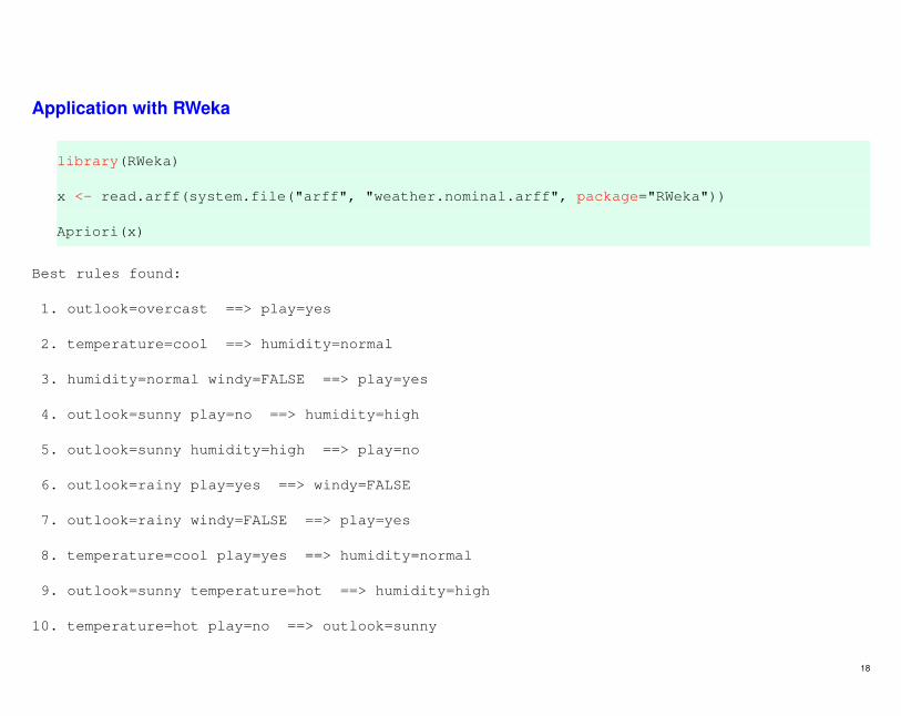
Application with RWeka

library(RWeka)

x <- read.arff(system.file("arff", "weather.nominal.arff", package="RWeka"))

Apriori(x)

Best rules found:

1. outlook=overcast ==> play=yes

2. temperature=cool ==> humidity=normal

3. humidity=normal windy=FALSE ==> play=yes

4. outlook=sunny play=no ==> humidity=high

5. outlook=sunny humidity=high ==> play=no

6. outlook=rainy play=yes ==> windy=FALSE

7. outlook=rainy windy=FALSE ==> play=yes

8. temperature=cool play=yes ==> humidity=normal

9. outlook=sunny temperature=hot ==> humidity=high

10. temperature=hot play=no ==> outlook=sunny

18

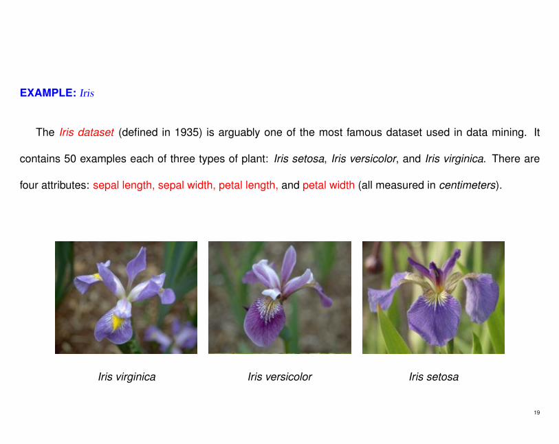
EXAMPLE: Iris

The Iris dataset (defined in 1935) is arguably one of the most famous dataset used in data mining. It

contains 50 examples each of three types of plant: Iris setosa, Iris versicolor, and Iris virginica. There are

four attributes: sepal length, sepal width, petal length, and petal width (all measured in centimeters).

Iris virginica Iris versicolor Iris setosa

19

Sepal length Sepal width Petal length Petal width Type

1 5.1 3.5 1.4 0.2 Iris setosa

2 4.9 3.0 1.4 0.2 Iris setosa

3 4.7 3.2 1.3 0.2 Iris setosa

4 4.6 3.1 1.5 0.2 Iris setosa

...

51 7.0 3.2 4.7 1.4 Iris versicolor




...

102 5.8 2.7 5.1 1.9 Iris virginica

103 7.1 3.0 5.9 2.1 Iris virginica

104 6.3 2.9 5.6 1.8 Iris virginica

105 6.5 3.0 5.8 2.2 Iris virginica

20

All attributes have values that are numeric. The following set of rules might be learned from this dataset:

If petal length < 2.45 then Iris setosa

If sepal width < 2.10 then Iris versicolor

If sepal width < 2.45 and petal length < 4.55 then Iris versicolor

If sepal width < 2.95 and petal width < 1.35 then Iris versicolor

If petal length >= 2.45 and petal length < 4.45 then Iris versicolor

If sepal length >= 5.85 and petal length < 4.75 then Iris versicolor

If sepal width < 2.55 and petal length < 4.95 and

petal width < 1.55 then Iris versicolor

If petal length >= 2.45 and petal length < 4.95 and

petal width < 1.55 then Iris versicolor

....

21

DEFINITIONS: Concepts, Instances, and Attributes

• The input values take the form of instances, attributes and concepts.

• In general, Information takes the form of a set of instances. In the previous examples, each instance

was an object or an individual.

• Each instance is characterized by the values of attributes that measure different aspects of the instance.

• There are many different types of attributes, although typical data mining methods deal only with nu-

meric and nominal (categorical) ones.

22

• In classification learning, the learning scheme is presented with a set of classified examples from

which it is expected to learn a way of classifying unseen examples.

• In association learning, any association among features is sought, not just ones that predict a parti-

cular class value.

• In clustering, groups of examples that belong together are sought.

• In numeric prediction, the outcome to be predicted is not a discrete class but a numeric quantity.

• Regardless of the type of learning involved, it is defined what must be learned as the concept , and the

output produced by a learning scheme is defined as the concept description.

• Example: the weather example is a classification problem. It presents a set of days together with a

decision for each as to whether to play the game or not.

23

• Classification learning is sometimes called supervised because the method operates under super-

vision. It is provided the actual outcome for each of the training examples.

• The outcome is called the class of the example.

• The success of classification learning can be determined by trying out the concept description that is

learned, on an independent set of test data for which the true classifications are known.

• The success rate on test data gives an objective measure of how well the concept has been learned.

• In association learning there is no a specified class. The problem is to discover any structure in the

data that is interesting.

• Association rules differ from classification rules in two ways: they can predict any attribute, not just

the class, and they can predict more than one attribute’s value at a time.

24

• Association rules usually involve only non-numeric attributes. Thus, for example, you would not nor-

mally look for association rules in the Iris dataset .

• When there is no specified class, clustering is used to group items that seem to fall naturally together.

• Imagine a version of the Iris data in which the type of Iris is omitted. Then it is likely that the 150

instances fall into natural clusters corresponding to the three Iris types.

• The challenge is to find these clusters and assign the instances to them, and to be able to assign new

instances to the clusters as well.

• It may be that one or more of the Iris types splits naturally into subtypes, in which case the data will

exhibit more than three natural clusters.

25

• Clustering may be followed by a second step of classification learning, in which rules that are learned

give an intelligible description about how new instances should be placed into the clusters.

• Numeric prediction is a variant of classification learning in which the outcome is a numeric value

rather than a category.

• With numeric prediction problems, the predicted value for new instances is often of less interest than

the structure of the description that is learned. This structure is expressed in terms of which are the

important attributes and how they relate to the numeric outcome.

26

Association rules

• Small example from the supermarket domain: Consider a set of products (items) I = {milk, bread,

butter, beer} and a small database of possible purchases (transactions) containing the items with 1

codes for presence, and 0 for absence of an item.

• Notations: Let I = {i1, i2, . . . , in} be a set of n binary attributes called items and D = {t1, t2, . . . , tm}

be a set of transactions called the database.

• Each transaction in D has a unique transaction identification ID and contains a subset of the items in I.

• A rule is defined as an implication of the form X ⇒ Y where X, Y ⊂ I and X ∩ Y = ∅.

• The sets of items (for short itemsets) X and Y are called antecedent (left-hand-side or LHS) and

consequent (right-hand-side or RHS) of the rule respectively.

27

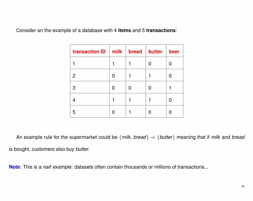
Consider an the example of a database with 4 items and 5 transactions:

transaction ID milk bread butter beer

1 1 1 0 0

2 0 1 1 0

3 0 0 0 1

4 1 1 1 0

5 0 1 0 0

An example rule for the supermarket could be {milk, bread} ⇒ {butter} meaning that if milk and bread

is bought, customers also buy butter.

Note: This is a naif example: datasets often contain thousands or millions of transactions...

28

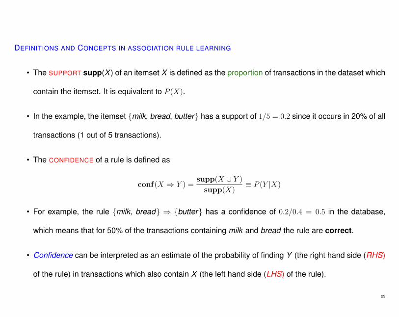
DEFINITIONS AND CONCEPTS IN ASSOCIATION RULE LEARNING

• The SUPPORT supp(X ) of an itemset X is defined as the proportion of transactions in the dataset which

contain the itemset. It is equivalent to P (X).

• In the example, the itemset {milk, bread, butter} has a support of 1/5 = 0.2 since it occurs in 20% of all

transactions (1 out of 5 transactions).

• The CONFIDENCE of a rule is defined as

conf(X ⇒ Y ) =supp(X ∪ Y )

supp(X)≡ P (Y |X)

• For example, the rule {milk, bread} ⇒ {butter} has a confidence of 0.2/0.4 = 0.5 in the database,

which means that for 50% of the transactions containing milk and bread the rule are correct.

• Confidence can be interpreted as an estimate of the probability of finding Y (the right hand side (RHS)

of the rule) in transactions which also contain X (the left hand side (LHS) of the rule).

29

• The LIFT of a rule is defined as

lift(X ⇒ Y ) =supp(X ∪ Y )

supp(X)× supp(Y )≡ P (X and Y )/P (X) · P (Y )

It is the the ratio of the observed support to what expected if X and Y were independent.

The rule {milk, bread} ⇒ {butter} has a lift of 0.20.4×0.4

= 1.25

• The CONVICTION of a rule is defined as

conv(X ⇒ Y ) =1− supp(Y )

1− conf(X ⇒ Y )≡ P (X)P (not Y )/P (X and not Y )

Conviction is the ratio of the probability of X occurs without Y if they were independent, with respect to

the probability of incorrect predictions.

• The rule {milk, bread} ⇒ {butter} has a conviction of 1−0.41−0.5

= 1.2. Then, if the association between X

and Y were purely at random, the rule would be incorrect 20% more often.

30

Example with arules

• We use the Adult data set from the UCI machine learning repository (Asuncion and Newman, 2007)

provided by the package arules. The data originates from the U.S. census bureau database and

contains 48842 observations with 14 attributes like age, work class, education, etc.

• In the original applications of the data, the attributes were used to predict the income level of individuals.

Here it is added the attribute income with levels small and large, representing an income of

≤ 50, 000$ and > 50, 000$, respectively.

library(arules)

data(AdultUCI)

dim(AdultUCI)

head(AdultUCI)

• AdultUCI has categorical and quantitative attributes and needs some preparations before it is suitable

for association mining with arules.

31

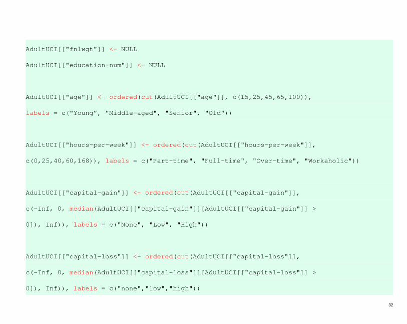
AdultUCI[["fnlwgt"]] <- NULL

AdultUCI[["education-num"]] <- NULL

AdultUCI[["age"]] <- ordered(cut(AdultUCI[["age"]], c(15,25,45,65,100)),

labels = c("Young", "Middle-aged", "Senior", "Old"))

AdultUCI[["hours-per-week"]] <- ordered(cut(AdultUCI[["hours-per-week"]],

c(0,25,40,60,168)), labels = c("Part-time", "Full-time", "Over-time", "Workaholic"))

AdultUCI[["capital-gain"]] <- ordered(cut(AdultUCI[["capital-gain"]],

c(-Inf, 0, median(AdultUCI[["capital-gain"]][AdultUCI[["capital-gain"]] >

0]), Inf)), labels = c("None", "Low", "High"))

AdultUCI[["capital-loss"]] <- ordered(cut(AdultUCI[["capital-loss"]],

c(-Inf, 0, median(AdultUCI[["capital-loss"]][AdultUCI[["capital-loss"]] >

0]), Inf)), labels = c("none","low","high"))

32

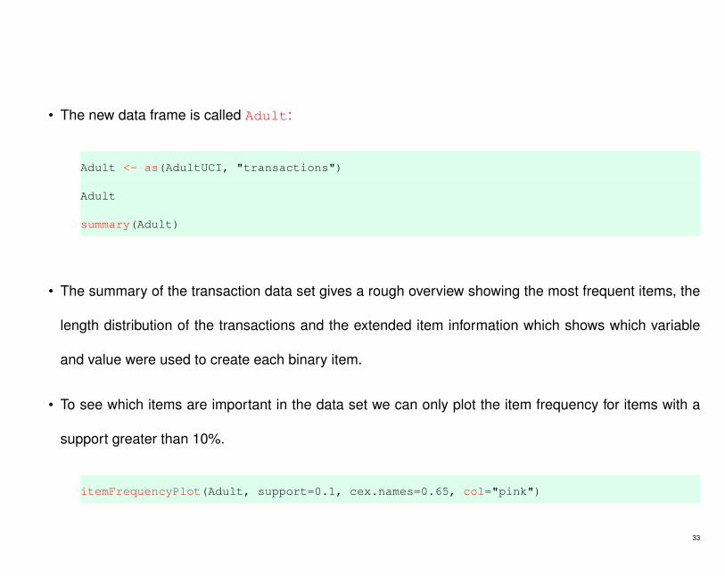
• The new data frame is called Adult:

Adult <- as(AdultUCI, "transactions")

Adult

summary(Adult)

• The summary of the transaction data set gives a rough overview showing the most frequent items, the

length distribution of the transactions and the extended item information which shows which variable

and value were used to create each binary item.

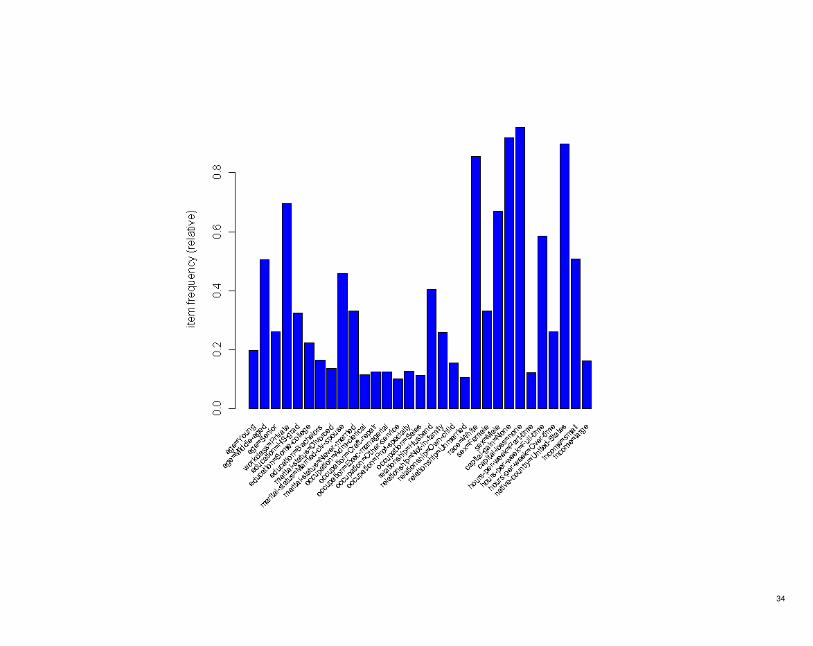
• To see which items are important in the data set we can only plot the item frequency for items with a

support greater than 10%.

itemFrequencyPlot(Adult, support=0.1, cex.names=0.65, col="pink")

33

• Next, we call the function apriori to find all rules with a minimum support of 1% and a confidence of

0.6.

rules <- apriori(Adult, parameter=list(support=0.01, confidence=0.6))

rules

• First, the function prints the used parameters. The parameter maxlen (maximum size of the mined

frequent itemsets) is by default restricted to 5. Longer association rules are only mined if maxlen is

set to a higher value.

• The result of the mining algorithm is a set of 276443 rules. For an overview of the mined rules summary

can be used. It shows the number of rules, the most frequent items contained in the left-hand-side

(LHS) and the right-hand-side (RHS) and their respective length distributions and summary statistics

for the quality measures returned by the mining algorithm.

summary(rules)

35

• As typical for association rule mining, the number of rules found is huge. It is useful to to produce

separate subsets of rules with the command subset. Consider variable income in the right-hand-side

(RHS) of the rule, and a lift value greater than 1.2.

rulesIncomeSmall <- subset(rules, subset=rhs %in% "income=small" & lift>1.2)

rulesIncomeLarge <- subset(rules, subset=rhs %in% "income=large" & lift>1.2)

• We now have a set with rules for persons with a small income and a set for persons with a large

income. For comparison, we inspect for both sets the three rules with the highest confidence, using

sort().

inspect(head(sort(rulesIncomeSmall, by="confidence"), n=3))

inspect(head(sort(rulesIncomeLarge, by="confidence"), n=3))

• From the rules we see that workers in the private sector working part-time, or in the service industry,

tend to have a small income. While persons with high capital gain who are born in the US tend to

have a large income.

36

Graphing rules with arulesViz

It is possible also to plot the obtained rules by using schemes:

library(arulesViz)

plot(head(sort(rulesIncomeSmall, by="confidence"), n=3),

method="graph",control=list(type="items"))

plot(head(sort(rulesIncomeLarge, by="confidence"), n=3),

method="graph",control=list(type="items"))

37

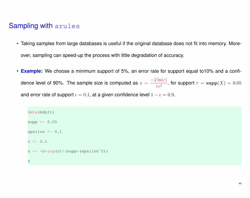
Sampling with arules

• Taking samples from large databases is useful if the original database does not fit into memory. More-

over, sampling can speed-up the process with little degradation of accuracy.

• Example: We choose a minimum support of 5%, an error rate for support equal to10% and a confi-

dence level of 90%. The sample size is computed as n =−2 ln(c)τε2

, for support τ = supp(X) = 0.05

and error rate of support ε = 0.1, at a given confidence level 1− c = 0.9.

data(Adult)

supp <- 0.05

epsilon <- 0.1

c <- 0.1

n <- -2*log(c)/(supp*(epsilonˆ2))

n

40

• With sample we produce a sample of size n with replacement from the database.

# n=9210.34

AdultSample <- sample(Adult, n, replace=TRUE)

• The sample can be compared with the original database (the population), by using an item frequency

plot. The item frequencies in the sample are displayed as bars, and the item frequencies in the original

database are represented by a line.

itemFrequencyPlot(AdultSample, population=Adult, support=supp, cex.names=0.7)

• It is obtained in this example, that mining the sample instead of the whole data base results in a speed-

up factor of roughly 5.

41

• To evaluate the accuracy for the itemsets mined from the sample, we analyze the difference between

the two sets.

itemsets <- eclat(Adult, parameter=list(support=supp), control=list(verbose=FALSE))

itemsetsSample <- eclat(AdultSample, parameter=list(support=supp),

control=list(verbose=FALSE))

itemsets

itemsetsSample

• The two sets have roughly the same size. To check if the sets contain similar itemsets, we match the

sets and see what fraction of frequent itemsets found in the database were also found in the sample.

matching <- match(itemsets, itemsetsSample, nomatch=0)

sum(matching > 0)/length(itemsets)

42

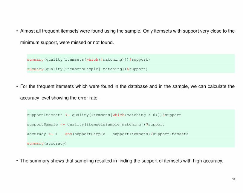
• Almost all frequent itemsets were found using the sample. Only itemsets with support very close to the

minimum support, were missed or not found.

summary(quality(itemsets[which(!matching)])$support)

summary(quality(itemsetsSample[-matching])$support)

• For the frequent itemsets which were found in the database and in the sample, we can calculate the

accuracy level showing the error rate.

supportItemsets <- quality(itemsets[which(matching > 0)])$support

supportSample <- quality(itemsetsSample[matching])$support

accuracy <- 1 - abs(supportSample - supportItemsets)/supportItemsets

summary(accuracy)

• The summary shows that sampling resulted in finding the support of itemsets with high accuracy.

43

introduction to data mining -...

Documents