Introduction to Cosmology

Joao G. Rosajoao.rosa@ua.pt

http://gravitation.web.ua.pt/cosmo

LECTURE 1 - The observed Universe

Cosmology is a fascinating subject that has witnessed an explosion of activity during the past decades with moreand more precision data becoming available with both ground- and space-based astrophysical observations. Its greatappeal for both theoretical and experimental physicists is associated with the broad range of physical processesrequired for a description of the observable universe and its dynamical evolution, bringing together a large numberof different concepts in gravitational and nuclear/particle physics.

The purpose of this course is to give an introductory overview to modern topics in cosmology, in particular theextremely successful Hot Big Bang model that defines the standard paradigm for the description of the universe fromits early stages to the present day. The discussion will be mostly self-contained but requires some basic knowledgeof Einstein’s theory of general relativity, quantum field theory and thermodynamics, although we will review thenecessary concepts as we proceed.

In this first lecture I will start by giving an overview of what we know about our Universe and the observationalgrounds on which the Hot Big Bang model stands. The remainder of this course will have a more theoretical approach,but the various observations that we will discuss in this lecture will become relevant as we explore different aspectsof the cosmological evolution. This is not intended as a comprehensive review of observational cosmology, but ratheras a description of the basic principles derived from observation that allow us to derive the standard cosmologicalparadigm.

Cosmological expansion

The most fundamental fact in modern cosmology is that the Universe is expanding, a critical discovery made byEdwin Hubble, working at the Mount Wilson Observatory, California, in 1929.

In the beginning of the 20th century, the prevailing picture of the Universe was very different from the one wehave today, and astronomers were still struggling to determine the size of our own galaxy, originally thought to beno more than a few tens of thousands of light years across, with the solar system occupying a fairly central position.Shapley dramatically changed this picture by using Cepheid variables to determine the distance to globular clusterswithin our galaxy. Cepheid stars, named after the constellation where they were originally found, are pulsating giantstars that can be used as standard candles, since their absolute luminosity can be determined from the period ofvariation of their brightness1. As the apparent magnitude of a star should decrease with the square of its distanceto the observer, one may infer the luminosity distance

dL =

(L

4πF

)1/2

(1)

from the absolute luminosity L and the observed flux F . Using this technique, Shapley showed that our galaxy wasin fact tens or even hundreds of times larger than previously estimated and could in fact contain the entire Universe,with the Sun significantly displaced from its centre.

1This relation can be calibrated using nearby Cepheids whose distance is measured by paralax, i.e. measuring the shift in position ofa star in the sky at different times of the year.

1

At the time, however, astronomers already knew the existence of faint nebulous objects known as nebulae andthat could be resolved into groups of stars. Hubble found a Cepheid variable in the Andromeda nebulae M31 andused Shapley’s technique to show that it was about 300 000 parsecs away (1 pc ' 3.6 ly ' 3.1× 1016 m) and so wellbeyond the established limits of our own galaxy. Hubble identified several other Cepheid variables and convincinglyshowed that nebulae were in fact island universes or independent galaxies as we know them today.

The even more revolutionary proposal that the universe is expanding came later on when Hubble and his studentMilton Humason combined distance and velocity measurements for spiral nebulae. Velocities can be computed fromthe Doppler shift of the spectral lines of these nebulae, a technique pioneered by Percival Lowell and his assistant VestoSlipher. Hubble determined that most galaxies, except for a few nearby ones which we now know are gravitationallybound to the Milky Way, are moving away from us since their spectral lines are redshifted. Moreover, the moredistant galaxies were receding at a faster rate than the nearby ones. The following figure shows Hubble’s originaldiagram, from which he inferred a linear relation between distance and velocity.

Figure 1: Hubble’s original diagram with the relation between velocity and distance [1] (left) and the modern Hubblediagram obtained using the Hubble Space Telescope [2] (right).

Although it is somewhat surprising that Hubble derived a linear relation from his original data, observationscollected over the years came to confirm his conclusion, as shown on the right panel of the figure above, and drasticallymodified our view of the Universe. This relation implies that galaxies are not just moving away from us, as if theMilky Way occupied a central position in the Universe, but that space itself must be expanding.

x=-1 x=0 x=1 x=2

Figure 2: One-dimensional toy universe with fixed galaxies labelled by a coordinate x with neighbouring galaxiesseparated by a distance a(t).

This can be seen in a simple one dimensional toy-model, where galaxies are placed at equal distance a from eachother and labelled by a fixed coordinate x. If space itself is expanding the scale factor will depend on time a = a(t)and the relative velocity between two galaxies at distance d = a∆x apart is simply v = a∆x, such that:

v =a

ad = Hd . (2)

2

The proportionality factor H is known as the Hubble constant or, more correctly, the Hubble parameter. It is aconstant in the sense that it does not depend on the particular galaxies one is considering, although it may (and aswe will see it does) vary in time. We can easily convince ourselves that this argument can be easily extended intothree dimensions if one assumes homogeneity and isotropy, as we discuss below. Of course galaxies are not exactlyat fixed coordinate distances in the real Universe and exhibit peculiar velocities that can be accurately measured,but this simple model illustrates how space itself must be expanding in order to explain the Hubble law.

We now know that the present value of the Hubble parameter is significantly different from Hubble’s original

determination of about 500 kms−1Mpc−1

, which was plagued with several systematic errors, and is measured to be[3]:

H0 = 100h kms−1Mpc−1

, h = 0.704± 0.025 , (3)

where h has conventionally been used to express the uncertainty in the measurement.The idea of an expanding Universe had been around even before Hubble announced his results, with the advent

of Einstein’s theory of general relativity describing space-time as a dynamical continuum evolving according to thelocal content of energy and momentum. Solutions to Einstein’s equations corresponding to expanding universeshad in fact been found by Willem de Sitter, Alexander Friedmann and Georges Lemaıtre, but the general opinion,including Einstein himself, was that the real Universe should be static. Einstein is in fact famous for introducing a“cosmological constant” term in his gravitational field equations to stabilize the ubiquitous non-static solutions, andafter Hubble’s discovery he came to acknowledge this as his “biggest blunder”. As we will see later on, Einstein’s“mistake” turned out to yield one of the most interesting puzzles in modern cosmology.

The fact that the Universe is presently expanding implies that it was much smaller in the past and the logicalextrapolation is that it must have emerged from a very hot and dense state, or even in fact an initial singularity ofinfinite density and temperature that was dubbed the ‘Big Bang’. The laws of physics have only been tested up toenergies of about 1 TeV, a boundary that is now being pushed at the Large Hadron Collider, in CERN, so that anydescription of the Universe at temperatures above this threshold is presently no more than theoretical speculation.The term ‘Big Bang’ has nevertheless been used since the 1950’s to denote the standard cosmological paradigm.

Large scale homogeneity and isotropy

The picture of the Universe proposed by Hubble and subsequently developed by many other physicists and as-tronomers depicts a world where all galaxies are drifting away from each other at the same rate at a given time,where no observer occupies a special place in the Universe - very far from the geocentric view that prevailed for somany centuries. Homogeneity and isotropy are also two key features of the standard cosmological paradigm and aconsequence of the so-called cosmological principle that the universe looks the same everywhere to all observers.

The assumption of homogeneity and isotropy goes back to Einstein’s original work, based on theoretical simplicityrather than any firm observational grounds. However, there is ample evidence for an isotropic and homogeneousuniverse within the presently observable universe, whose size is determined by the present Hubble radius cH−1

0 '3000h−1 Mpc as we will see in the next lecture. Of course the sky does not exactly look the same everywhere andwe can easily identify our own Milky Way. Homogeneity and isotropy are properties of the Universe on large scales,greater than a few tens of Mpc.

The best evidence we have for large-scale homogeneity and isotropy comes from measuring the Cosmic MicrowaveBackground (CMB) radiation, a relic of the Big Bang that we will discuss below that yields the most perfect blackbody spectrum ever found. The temperature of the CMB is basically uniform throughout the sky, exhibiting tinyfluctuations of the order of 1 part in 100 000 that are crucial to our understanding of the energy density profile inthe early Universe.

Additional evidence for a homogeneous and isotropic Universe comes from the X-ray background (to about 5%),the distribution of faint radio sources and that of galaxies themselves. Large galaxy surveys have been performed inthe past decade, such as the Sloan Digital Sky Survey (SDSS) and the 2dF Galaxy Redshift Survey, that measuredthe spectra of hundreds of thousands of objects and obtained precise three-dimensional maps of the deep sky. Thestatistical distribution of galaxies in these surveys indeed exhibits a large degree of isotropy and homogeneity onscales of a few to almost 100 Mpc.

3

Measurements of the peculiar velocity field in the Universe, i.e. of galactic velocities subtracted of the Hubbleflow, have also given some (rough) evidence for homogeneity on scales as large as 60h−1 Mpc, yielding local matterinhomogeneities of the order of δρ/ρ ∼ 0.1.

Age of the Universe

The Hubble constant sets a time scale H−10 ' 9.8h−1 Gyr. As we will see in the next lectures, the knowledge of

the present expansion rate and the matter and energy content of the Universe allows one to determine its age, i.e.to extrapolate back in time to determine the moment of the primordial ‘bang’ For example, in a matter-dominatedmodel one finds t0 = (2/3)H−1

0 , with more complicated expressions if the Universe is filled with different forms ofmatter, radiation and other exotic forms of energy. The age of the Universe thus provides an important test ofcosmological models, and the presently accepted value is of 13.77± 0.13 Gyr [3].

Hubble’s original determination of the expansion rate, which we know today differs significantly from thepresently measured value, place the age of the Universe at around 2 Gyr, which created a huge problem for cosmo-logical models, since this was less than the estimated age of the solar system of about 4.5 Gyr. This “age crisis”motivated the birth of alternative theories such as the steady state cosmology, proposed by Hoyle, Bondi and Gold,where an ‘ageless’ and unchanging universe resulted from the continuous creation of matter and energy. Interest-ingly, Fred Hoyle was the one to coin the term ‘Big Bang’ in 1950, as a kind of mockery of what he thought wasan “irrational” way of describing the Universe. We now know that the current measurements of the expansion rateare consistent with other methods of determining the age of the Universe and that the Big Bang model has passedinumerous observational tests with flying colours, whereas the unchanging steady-state cosmology fails for exampleto explain the origin of the CMB.

The age of the Universe can be determined, or at least constrained, by several other different methods, such as:

• the age of oldest globular clusters, which can be determined by looking at the transition from main sequenceto red giant phase stars in the corresponding Hertzprung-Russell diagram;

• astrophysical abundances of radioactive isotopes, in particular elements produced by fast neutron capture(r-process) in an early generation of stars such as Uranium isotopes;

• cooling time for white dwarf stars.

All these techniques have inherent difficulties and associated errors but are consistent with a Universe between10 and 20 Gyr old.

Light-element abundances

In 1946, George Gamow and Ralph Alpher used the recent developments in nuclear physics to make detailed cal-culations of nuclear reaction rates in the early universe. They assumed the Universe evolved from an initial stateof an infinite density and temperature by expanding and cooling, such that stable nuclei could be formed from aprimordial soup of protons, neutrons and electrons that they called ‘Ylem’, from a medieval word for matter. Underthese assumptions they were able to predict correctly the observed abundances of Hydrogen and Helium, the latteraccounting for a quarter of the luminous matter in the Universe and the former for almost all remaining mass.Primordial nucleosynthesis or Big Bang nucleosynthesis (BBN) is the earliest and one of the most stringent testsof Big Bang cosmology, with the relevant nuclear reactions taking place from t ' 0.01 to 100 sec, corresponding totemperatures of T ' 10 MeV to 0.1 MeV.

Alpher and Gamow’s results for the abundances of light elements were extremely successful and the primordialsoup is able to produce substantial amounts of Deuterium (D/H ∼ 10−5), 3He (3He/H ∼ 10−5), 4He (mass fractionY ' 0.25) and 7Li (7Li/H ∼ 10−10). Helium and deuterium are of particular importance, since there are nocontemporary astrophysical processes that are capable of producing the observed amounts - the contribution ofstellar processing to the 4He abundance can be at most 5% in particular environments and even such a smallabundance of Deuterium would be easily destroyed in stellar cores at temperatures of several million Kelvin, since itis very weakly bound. However, BBN cannot produce considerable amounts of elements heavier than Helium, which

4

was originally seen as an argument against the Hot Big Bang model. Today we know that heavier elements canbe produced in stellar interiors and supernovae explosions, accounting for the observed abundances, so that BBN istruly a remarkable success of Big Bang cosmology.

The predicted abundances of the light elements depend on the baryon-to-photon ratio η, i.e. the ratio betweenthe number of ordinary nucleons such as protons and neutrons and the number of light particles. The observedabundances then imply η ' 5−7×10−10. This corresponds to the number of baryons that have not annihilated withtheir corresponding anti-particles within the primordial soup and one of the main challenges in modern cosmology,which we will address later on, is to explain how such a small but non-vanishing number arises. This typicallyrequires non-trivial extensions of the Standard Model of particle physics and is an area of active research.

3He/H p

4He

2 3 4 5 6 7 8 9 101

0.01 0.02 0.030.005

CMB

BBN

Baryon-to-photon ratio ! " 10#10

Baryon density $Bh2

D___H

0.24

0.23

0.25

0.26

0.27

10#4

10#3

10#5

10#9

10#10

2

57Li/H p

Yp

D/H p

Figure 3: Light-element abundances predicted by Big Bang nucleosynthesis. Boxes indicate the observed light elementabundances (smaller boxes: 2σ statistical errors; larger boxes: ±2σ statistical and systematic errors). The narrowvertical band indicates the CMB measure of the cosmic baryon density [4].

The success of BBN also poses severe constraints on any departures from standard cosmology in the temperaturerange mentioned above, in particular constraining the existence of additional light particle species (. MeV) commonin many extensions of the Standard Model. Although we will not explore this possibility in detail during this course,it is worth mentioning that the BBN prediction for the abundance of Lithium is about 3-4 times larger than what isobserved in old stars in the Milky Way halo, which constitutes the modern ‘Lithium problem’ and may require some(minor) modification of the standard cosmological evolution [5].

Cosmic Microwave Background

The CMB is perhaps the best evidence we have for the Hot Big Bang paradigm and at the same time the best toolfor precision measurements in cosmology. As opposed to e.g. the steady state model discussed previously, in theHot Big Bang model the Universe cools down as it expands and the density of matter and energy decreases. Asfirst predicted by Ralph Alpher and Robert Herman in 1948, when the Universe was about 379 000 years old, the

5

temperature of the Universe was about 3000 K, which is sufficiently low for protons and electrons to combine intoneutral atoms. At this point, photons - the quanta of light - stopped interacting with matter and became allowedto travel freely through space. This is called the epoch of recombination and decoupling and also referred to as thelast scattering surface, since light from this epoch has basically remained unaltered to the present day. The Universeremained basically neutral until much later when the first stars formed and their light broke some of the neutralatoms into Hydrogen ions in the interstellar medium - this is called the epoch of reionization.

The CMB was discovered in 1964 by two American radio astronomers, Arno Penzias and Robert Wilson, whowere later awarded the 1978 Nobel Prize in Physics. Penzias and Wilson accidentally found a faint background ofradiation in the microwave range while working in the detection of radio waves bounced off echo balloon satellites.This mysterious noise seem to be evenly distributed throughout the sky, did not originate from any known sourceand persisted even after a family of pigeons nesting in their antenna were carefully evicted and their droppingsremoved - what Penzias amusingly described as “white dielectric material”. At the same time, a group of Princetonastrophysicists including Jim Peebles, Robert Dicke and David Wilkinson were preparing to search for microwaveradiation in this range, realizing that the relic radiation from the Big Bang should be redshifted by expansion andpresently lie in this part of the electromagnetic spectrum. When they learned about Penzias and Wilson’s observationit became clear that it must correspond to the CMB - the definitive evidence in favour of a Hot Big Bang model asopposed to the competing steady state hypothesis.

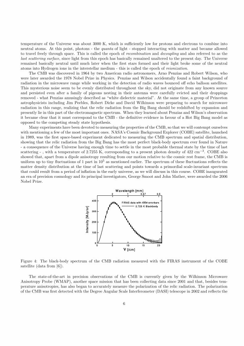
Many experiments have been devoted to measuring the properties of the CMB, so that we will contempt ourselveswith mentioning a few of the most important ones. NASA’s Cosmic Background Explorer (COBE) satellite, launchedin 1989, was the first space-based experiment dedicated to measuring the CMB spectrum and spatial distribution,showing that the relic radiation from the Big Bang has the most perfect black-body spectrum ever found in Nature- a consequence of the Universe having enough time to settle in the most probable thermal state by the time of lastscattering - , with a temperature of 2.7255 K, corresponding to a present photon density of 422 cm−3. COBE alsoshowed that, apart from a dipole anisotropy resulting from our motion relative to the cosmic rest frame, the CMB isuniform up to tiny fluctuations of 1 part in 105 as mentioned earlier. The spectrum of these fluctuations reflects thematter density distribution at the time of last scattering and points towards a primordial scale-invariant spectrumthat could result from a period of inflation in the early universe, as we will discuss in this course. COBE inauguratedan era of precision cosmology and its principal investigators, George Smoot and John Mather, were awarded the 2006Nobel Prize.

Figure 4: The black-body spectrum of the CMB radiation measured with the FIRAS instrument of the COBEsatellite (data from [6]).

The state-of-the-art in precision observations of the CMB is currently given by the Wilkinson MicrowaveAnisotropy Probe (WMAP), another space mission that has been collecting data since 2001 and that, besides tem-perature anisotropies, has also began to accurately measure the polarization of the relic radiation. The polarizationof the CMB was first detected with the Degree Angular Scale Interferometer (DASI) telescope in 2002 and reflects the

6

distribution of charge at last scattering, being one of the most promising observables in modern cosmology. WMAPhas recently released its final 9-year observation results with tight constraints on cosmological parameters, but willsoon be overthrown by the European Planck mission, launched in 2009 and expected to bring precision cosmologyto a new level in early 2013.

Figure 5: CMB temperature sky maps obtained with the COBE satellite after 2 years of data collection (left) andwith the WMAP satellite after 9 years of data collection. The colour code corresponds to temperature fluctuationsof a few micro-Kelvin about the uniform 2.7255 K background, after the Milky Way foreground has been removed[7].

Visible and dark matter

An important observable in cosmology is the amount of matter present in the Universe, since as we will see thisdetermines the expansion rate and consequently the cosmological evolution. In theory, the average density of theUniverse could be measured by determining the number of galaxies in the Hubble volume and the average galaxymass:

〈ρ〉 = nG〈MG〉 . (4)

The mass of a galaxy can be determined from its gravitational effect, in particular measuring distances and velocitiesof stars within the galaxy and using Kepler’s third Law:

GM(r) = v2r , (5)

where r is the distance to the galactic centre, v the orbital velocity and M(r) the total mass within a sphere of radiusr, assuming spherical symmetry. Using this technique for spiral galaxies and taking the largest distance within whichmost of the galaxy light is emitted, one finds that luminous matter provides less than 1% of the critical densityrequired for a flat Universe:

ρc =3H2

0

8πG= 1.88× 10−29h2 gcm−3 . (6)

The meaning of this critical density will become clearer later on this course, but for now it suffices to say thatobservations suggest that the Universe has in fact a very flat geometry, in particular the position of the first acousticpeak in the CMB power spectrum. This implies that luminous matter in galaxies cannot account for the matterdensity of our Universe!

Moreover, when the rotational curves of galaxies are extended beyond the above mentioned luminous boundary,for example by measuring velocities of rare stars or 21 cm emission from neutral Hydrogen gas clouds, one finds thatthese curves flatten, i.e. v ' const. at large distances, which from Eq. (5) implies M(r) ∝ r. Thus, there seemsto be a lot of “dark” mass extending beyond the visible limits of virtually all spiral galaxies, as first shown by JanOort in 1932 for the Milky Way, and there is (weak) evidence for it being spherically distributed, with ρDM ∝ r−2.This dark halo contributes at least 3 to 10 times the mass of visible matter and some fraction of it can be accountedfor by non-luminous baryonic matter, since BBN and CMB measurements indicate baryonic matter should yieldabout 4-5% of the critical density. This corresponds for example to “dark” objects such as Jupiter-like planets, white

7

dwarfs, neutron stars, black holes, etc. However, this means that most of the matter and energy in the Universe isunaccounted for!

The average galactic mass in a cluster of galaxies can also be determined by other means. Clusters aregravitationally-bound systems and, assuming they had sufficient time to relax, one can use the virial theorem toshow that:

GM = 2〈v2〉〈r−1〉

. (7)

Thus, measuring average velocity of galaxies and the average inverse distance between galaxies in a cluster can beused to infer its total gravitational mass, as first shown by Fritz Zwicky in 1933. This technique yields fractions ofthe critical density in clusters of about 10-30%, consistently with other techniques such as local distortions of theHubble flow. Measurements of the CMB anisotropy spectrum are perhaps the most accurate way of determining theamount of matter in the Universe, and the best fit to the data yields 24% of the critical density in pressureless cold(non-relativistic) dark matter, implying that the remaining 71% must correspond to an unknown component whichis ‘unclustered’, i.e. smoothly distributed, and which we briefly discuss below.

Non-baryonic dark matter is one of the most interesting puzzles in modern cosmology, pointing towards newelementary particles and extensions of the Standard Model of particle physics. A lot of effort has recently beendevoted to building theoretical models to describe this non-luminous component with the observed abundance andin devising experimental ways to directly and/or indirectly detect any dark matter particles flowing within our localenvironment. Although there are some interesting ‘hints’ for dark matter, the results have so far been inconclusiveand we will devote one of our final lectures to this topic. It is important to mention at this stage, however, thatalternative hypothesis such as modified theories of gravity are currently less widely accepted, in particular givenrecent weak-lensing maps of galaxy clusters, such as the Bullet cluster, where the separation between gravitationaland luminous mass is evident.

Figure 6: Image of the Bullet cluster obtained by the Chandra satellite. Shown in green are the gravitational masscontours reconstructed from weak-lensing observations [8].

Large-scale structure

As we have been discussing so far, on large scales the Universe is well-described by a homogeneous and isotropicmodel, but on smaller scales it exhibits several features and a particular structure from which we can learn a greatamount. In particular, as mentioned above, from the large galaxy surveys that have been performed in the pastdecade we have been able to learn a great deal about the distribution of matter in the Universe. Galaxies are,to a first approximation, distributed uniformly throughout the sky, but have a tendency to cluster. This can bequantified by the galaxy-galaxy correlation function, ξGG, defined as the probability in excess of a random (Poisson)distribution of finding two galaxies at a distance r apart. For distances 0.1h−1 Mpc . r . 16h−1 Mpc, the followingpower-law has been derived from the SDSS data [9]:

ξGG '(

r

6.1h−1 Mpc

)−1.75

. (8)

8

Also, about 10% of the observed galaxies are found in gravitationally-bound clusters, such as the nearby Virgoand Coma clusters. The Abell catalogue combines over 4000 galaxy clusters and classifies them according to theirrichness, which roughly corresponds to the number of galaxies in the cluster. A cluster-cluster correlation functionof the same form as Eq. (8) can be derived from this catalogue, valid for distances 10h−1 Mpc . r . 50h−1 Mpc:

ξCC '(

r

25h−1 Mpc

)−1.8

. (9)

More recent cluster data indicates a slightly smaller correlation length 16− 19h−1 Mpc and a slightly steeper power-law, depending on the richness class, but the difference between the correlation lengths in the galaxy and clustercorrelation functions seems to suggest that light may only be a ‘biased’ tracer of matter, which may give us importantclues on the distribution of dark matter in the Universe [10].

There are also seem to exist larger structures, such as superclusters which are more loosely-bound and non-virialized, with densities about twice the average density of the Universe. These include our own Local Supercluster,centered in Virgo, Hydra-Centaurus and Pisces-Cetus. On the opposite end, large voids with virtually no matter(luminous or dark) have been found in the surveys, ranging from 10 − 100 Mpc in diameter, the largest confirmedone being the Bootes void, which is about 75 − 100 Mpc across. Even larger voids are conjectured to exist, inparticular the ‘Great Void’ or ‘Eridanus Supervoid’, which could be associated with ‘cold spot’ observed in the CMBtemperature anisotropy distribution.

Figure 7: The galaxy distribution obtained from spectroscopic redshift surveys and from mock catalogues constructedfrom cosmological simulations [12].

A lot of progress has also been made in modeling the growth of structure in the Universe using N -body numericalsimulations, performed for example by the Millenium or the more recent DEUS collaborations (see e.g.[11] for a recentreview). These simulations follow the (non-linear) gravitational evolution of a primordial density profile of collisionlesscold dark matter particles and have shown the formation of different types of structures such as filaments, walls andvoids, in good agreement with observational data as illustrated in figure 7.

9

Besides galaxy surveys, other techniques are currently being used to study the large-scale structure of theUniverse, namely weak gravitational lensing and distant quasar absorption line (Lyman-α, etc) surveys, which willhopefully shed a new light on the difference between the dark and luminous matter distributions.

Evidence for acceleration

As we discussed previously, evidence for an expanding Universe requires determining distances and velocities ofstandard candles - objects for which the absolute luminosity is known or can be calibrated. The Cepheid variablesare the prime example of such objects and have been detected at distances as far as 10 Mpc. However, to determinethe expansion history of the Universe to earlier times, we need to find standard candles at distances at least 100times larger. Already in 1938, Baade and Zwicky proposed that supernovae could provide standard candles to verylarge distances, since they are extremely bright and, for a short period, can outshine a whole galaxy.

Type Ia supernovae are particularly suitable for this task, occurring in binary systems when a low-mass whitedwarf star accreting matter from a companion exceeds the Chandrasekhar limit of 1.4 solar masses and becomesunstable, leading to a thermonuclear explosion producing an enormous amount of energy and leaving a neutronstar remnant. Their brightness evolves over periods of a few weeks and, within our galaxy, supernovae can even beobserved with the naked eye, as recorded for example by Chinese astronomers in 1054! The spectra and light curvesof type Ia supernovae are extremely uniform, which indicates a common origin and absolute luminosity, which canbe determined from the relation between their peak brightness and decay time.

Although extremely rare events for a single galaxy, statistically significant samples of supernovae data havebeen collected since the 1990’s, in particular by the Supernova Cosmology Group (SCP), led by Saul Perlmutter ofthe Lawrence Berkeley National Laboratory (USA), and the High-z Supernova Search Team (HZT), led by BrianSchmidt of the Mount Stromlo Observatory in Australia. In the beginning of 1998, both groups published resultsfor redshift and distance measurements of 42 and 16 type Ia supernovae, respectively, the latter having analyzedmainly by Adam Riess, a postdoctoral researcher at UC Berkeley (USA). Their results were crucial in determiningthe extension of the Hubble law into large distances.

As we will derive later on, the relation between the luminosity distance and redshift in an expanding Universeis given by:

dL = H−10

(z +

1

2(1− q0)z2 + . . .

), (10)

where for a spectral line of wavelength λ1 emitted at time t1 and observed at time t0 with wavelength λ0 the redshiftis given by:

z =λ0 − λ1

λ1=a(t0)

a(t1)− 1 , (11)

with a(t) denoting the scale factor of the Universe, since waves simply stretch with expansion. As we can see, atlow-redshifts the linear Hubble law is recovered, while at larger redshifts some deviations may be expected, dependingon whether expansion is accelerating or decelerating. In principle, ordinary matter can only make expansion slowdown due to its gravitational pull, so that q0 = −a(t0)a(t0)/a2(t0) is historically known as the deceleration parameter.However, the data from the SCP and HZT groups, including supernovae up to z . 1, showed quite the opposite -high redshift supernovae are dimmer than expected with the linear Hubble law by a factor of about 10−15 %, whichmeans the Universe is unexpectely accelerating! For this surprising discovery, Perlmutter, Schmidt and Riess wereawarded the 2011 Nobel Prize in Physics.

Accelerated expansion cannot be produced by ordinary matter and radiation, in fact requiring an exotic fluidgenerically known as dark energy, and whose negative pressure counterbalances the gravitational attraction. Thesimplest example of dark energy is in fact Einstein’s cosmological constant, typically denoted by Λ, and whichcorresponds to vacuum energy. This creates a huge theoretical problem, as crude estimates of the quantum vacuumenergy in the Standard Model yield a cosmological constant which is about 120 orders of magnitude larger than thevalue required to explain the supernovae data!

10

Calan/Tololo (Hamuy et al, A.J. 1996)

Supernova Cosmology Project

effe

ctiv

e m

Bm

ag re

sidua

lsta

ndar

d de

viat

ion

(a)

(b)

(c)

(0.5,0.5) (0, 0)( 1, 0 ) (1, 0)(1.5,–0.5) (2, 0)

( , ) = ( 0, 1 )

Flat

(0.28, 0.72)

(0.75, 0.25 ) (1, 0)

(0.5, 0.5 ) (0, 0)

(0, 1 )( , ) =

= 0

redshift z

14

16

18

20

22

24

-1.5-1.0-0.50.00.51.01.5

0.0 0.2 0.4 0.6 0.8 1.0-6-4-20246

Figure 8: Hubble diagram obtained with 42 high-redshift type Ia supernovae from SCP and 18 low-redshift supernovaefrom the Calan-Tololo Supernova Survey. The solid and dashed curves corresponds to different cosmological modelswith different matter and cosmological constant abundances relative to the critical density, denoted by ΩM and ΩΛ,respectively [13].

11

The supernovae data is actually consistent with CMB and large-scale structure observations, and dark energyprovides the missing smooth component leading to a critical density in the Universe. The simplest model consistentwith the observational data so far is thus the so-called ΛCDM or concordance model, with the present energy densityof the Universe divided into 71% of dark energy (cosmological constant), 24% of cold dark matter and 5% of ordinarybaryonic matter. The agreement between this model and observations is remarkable, but it remains an enormoustheoretical challenge to explain the observed value of the cosmological constant and the so-called coincidence problem- dark energy only became the dominant component in the Universe very recently (on cosmological time scales!), asstudies of supernovae at z > 1 have confirmed that the Universe was matter-dominated at earlier times.

Figure 9: The concordance model or ΛCDM model putting together observations from type Ia supernovae, CMBtemperature anisotropies and large-scale structure, in particular the so-called baryon acoustic oscillations (BAO).The solid line corresponds to a flat Universe with matter and a cosmological constant ΩΛ + Ωm = 1 [14].

We will discuss possible models of dark energy in more detail in one of our last lectures, but it is important tomention at this stage that there are alternative models, such as inhomogeneous cosmologies. These models make useof the fact that the expansion rate is larger in overdense regions, so that if we happen to live inside a particularlylarge void in the Universe we will measure a lower value of H0 in our vicinity than the average value in the Universe(see e.g. [15]). Although other particle physics scenarios and modified gravity theories may also account for thesupernovae dimming, the dark energy hypothesis remains the most widely accepted possibility.

12

Summary

In summary, observations can tell us a lot about the properties, structure and evolution of Universe, covering itshistory as far back as 0.01 seconds. Cosmological observables thus include:

• the present Hubble parameter H0 and deceleration parameter q0

• the age of the Universe t0

• the present energy density ρ0 and composition (baryonic and dark matter, radiation, cosmological constant,etc)

• the CMB temperature and polarization spectra, as well as other cosmological background radiations (IR, UV,X-ray, γ-ray, etc)

• the cosmological abundance of light-elements (H, D, 3He, 4He, 7Li)

• the baryon-to-photon ration, η

• the statistical distribution of galaxies, clusters and larger structures

In the next lectures we will describe the standard cosmological paradigm based on these observables and towardsthe end of the course we will look at its shortcomings and open problems, and what they may tell us about particleand gravitational physics at high temperature/energy scales.

Problem 1

Assuming the virial theorem for a gravitationally-bound cluster of n 1 galaxies of equal mass mG, 〈K〉 = −〈V 〉/2,derive Eq. (7) that allows one to determine the total cluster mass M = nmG.

13

References

[1] R. P. Kirshner, Hubble’s diagram and cosmic expansion Proc. Natl. Acad. Sci. U S A 2004 101, 8 (2004).

[2] W. L. Freedman et al. [HST Collaboration], Final results from the Hubble Space Telescope key project to measurethe Hubble constant, Astrophys. J. 553, 47 (2001) [astro-ph/0012376].

[3] J. Beringer et al. [Particle Data Group Collaboration], Review of Particle Physics (RPP), Phys. Rev. D 86,010001 (2012).

[4] B. Fields and S. Sarkar, Big-Bang nucleosynthesis (2006 Particle Data Group mini-review), astro-ph/0601514.

[5] B. D. Fields, The primordial lithium problem, Ann. Rev. Nucl. Part. Sci. 61, 47 (2011) [arXiv:1203.3551 [astro-ph.CO]].

[6] J. C. Mather, E. S. Cheng, R. A. Shafer, C. L. Bennett, N. W. Boggess, E. Dwek, M. G. Hauser and T. Kelsallet al., A Preliminary measurement of the Cosmic Microwave Background spectrum by the Cosmic BackgroundExplorer (COBE) satellite, Astrophys. J. 354, L37 (1990).

[7] Data available from http://lambda.gsfc.nasa.gov

[8] D. Clowe, M. Bradac, A. H. Gonzalez, M. Markevitch, S. W. Randall, C. Jones and D. Zaritsky, A directempirical proof of the existence of dark matter, Astrophys. J. 648, L109 (2006) [astro-ph/0608407].

[9] I. Zehavi et al. [SDSS Collaboration], Galaxy clustering in early SDSS redshift data, Astrophys. J. 571, 172(2002) [astro-ph/0106476].

[10] T. Hong, J. L. Han, Z. L. Wen, L. Sun and H. Zhan, The correlation function of galaxy clusters and detectionof baryon acoustic oscillations, Astrophys. J. 749, 81 (2012) [arXiv:1202.0640 [astro-ph.CO]].

[11] M. Kuhlen, M. Vogelsberger and R. Angulo, Numerical Simulations of the Dark Universe: State of the Art andthe Next Decade, Phys. Dark Univ. 1, 50 (2012) [arXiv:1209.5745 [astro-ph.CO]].

[12] V. Springel, C. S. Frenk and S. D. M. White, The large-scale structure of the Universe, Nature 440, 1137 (2006)[astro-ph/0604561].

[13] S. Perlmutter et al. [Supernova Cosmology Project Collaboration], Measurements of Omega and Lambda from42 high redshift supernovae, Astrophys. J. 517, 565 (1999) [astro-ph/9812133].

[14] M. Kowalski et al. [Supernova Cosmology Project Collaboration], Improved Cosmological Constraints from New,Old and Combined Supernova Datasets, Astrophys. J. 686, 749 (2008) [arXiv:0804.4142 [astro-ph]].

[15] S. Nadathur and S. Sarkar, Reconciling the local void with the CMB, Phys. Rev. D 83, 063506 (2011)[arXiv:1012.3460 [astro-ph.CO]].

14