introduction to computer graphics ppt3: attributes of
TRANSCRIPT

1
EEL 5771-001
Introduction to Computer Graphics
PPT3: Attributes of Graphics Primitives
Team Mercedes
• Ajay Varma Chekuri (U35109473)
• Nithish Yarramasu (U65321808)
• Vishwoday Chirumalla (U86569920)
2
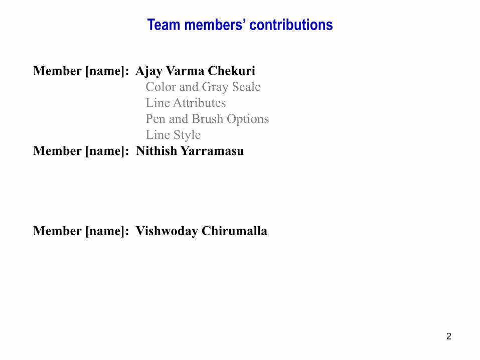
Team members’ contributions
Member [name]: Ajay Varma Chekuri
Color and Gray Scale
Line Attributes
Pen and Brush Options
Line Style
Member [name]: Nithish Yarramasu
Member [name]: Vishwoday Chirumalla
3
Color and Gray Scale
What is Gray Scale?
Gray Scale is a range of shades of gray without apparent
color. The darkest possible shade is black, which is the total
absence of transmitted or reflected light. The lightest possible
shade is white, the total transmission or reflection of light at
all visible wavelengths. Intermediate shades of gray are
represented by equal brightness levels of the three primary
colors (red, green and blue) for transmitted light, or equal
amounts of the three primary pigments (cyan, magenta and
yellow) for reflected light.

4
Color and Gray Scale
Bitmap Color Depth:
• Describes the amount of storage per pixel
• Also indicates the number of colors available
• Higher color depths require greater compression
When a bitmap image is constructed, the color of each point or pixel in the image is coded into a
numeric value. This value represents the color of the pixel, its hue and intensity. When the
image is displayed on the screen, these values are transformed into intensities of red, green and
blue guns inside the monitor . In fact, the screen itself is mapped out in the computer's memory,
stored as a bitmap from which the computer hardware drives the monitor.
These color values have to be finite numbers, and the range of colors that can be stored is known
as the color depth. The range is described either by the number of colors that can be
distinguished, or more commonly by the number of bits used to store the color value. Thus, a
pure black and white image (i.e. no greys) would be described as a 1-bit or 2-colour image,
since every pixel is either black (0) or white (1). Common color depths include 8-bit (256
colors) and 24-bit (16 million colors). It's not usually necessary to use more than 24-bit color,
since the human eye is not able to distinguish that many colors, though broader color depths
may be used for archiving or other high-quality work.

5
Color and Gray Scale
Eight-bit color stores the color of each pixel in eight binary digits (bits) which
gives 256 colors in total.

6
Color and Gray Scale
Twenty-four bits (three bytes) per pixel gives us a possible 16 million (approx.)
colors, which is more than the human eye can accurately distinguish.

7
Color and Gray Scale
Displaying gray-scale intensities:
Color output on printers is described with cyan, magenta, and yellow color
components, and color interfaces sometimes use parameters such as lightness and
darkness to choose a color. Also, color, and light in general, are complex subjects,
and many terms and concepts have been devised in the fields of optics,
radiometry, and psychology to describe the various aspects of light sources and
lighting effects
Physically, we can describe a color as electromagnetic radiation with a particular
frequency range and energy distribution, but then there are also the characteristics
of our perception of the color. Thus, we use the physical term intensity to
quantify the amount of light energy radiating in a particular direction over a
period of time, and we use the psychological term luminance to characterize the
perceived brightness of the light. We discuss these terms and other color concepts
in greater detail when we consider methods for modeling lighting effects and the
various models for describing color.

8
Color and Gray Scale
Photometry:
The human eye is not equally sensitive to all wavelengths of visible light. Photometry attempts
to account for this by weighing the measured power at each wavelength with a factor that
represents how sensitive the eye is at that wavelength. The standardized model of the eye's
response to light as a function of wavelength is given by the luminosity function. The eye has
different responses as a function of wavelength when it is adapted to light conditions (photopic
vision) and dark conditions (scotopic vision). Photometry is typically based on the eye's
photopic response, and so photometric measurements may not accurately indicate the perceived
brightness of sources in dim lighting conditions where colors are not discernible, such as under
just moonlight or starlight. Photopic vision is characteristic of the eye's response at luminance
levels over three candela per square meter. Scotopic vision occurs below
2 × 10⁻⁵ cd/m2. Mesopic vision occurs between these limits and is not well characterized for
spectral response.
A colorimetric (or more specifically photometric) grayscale image is an image that has a
defined grayscale colorspace, which maps the stored numeric sample values to the achromatic
channel of a standard colorspace, which itself is based on measured properties of human vision.

9
Color and Gray Scale
Dynamic Range:
It is the ratio between the largest and smallest values that a certain values that a certain quantity
can assume. The human sense of sight has a relatively higher dynamic range. However, a human
cannot perform these feats of perception at both extremes of the scale at the same time. The
human eye takes time to adjust to different light levels, and its dynamic range in a given scene is
actually quite limited due to optical glare.
To cover the dynamic range for nights, when showing a movie or a game, a display is able to
show both shadowy nighttime scenes and bright outdoor sunlit scenes, but in fact the level of
light coming from the display is much the same for both types of scenes. Knowing that the
display does not have a huge dynamic range, the producers do not attempt to make the nighttime
scenes accurately dimmer than the daytime scenes, but instead use other cues to suggest night or
day.
Photographers use dynamic range to describe the luminance range of a scene being
photographed, or the limits of luminance range that a given digital camera or film can
capture, or the opacity range of developed film images, or the reflectance range of images on
photographic papers.
The dynamic range of digital photography is comparable to the capabilities of photographic film
and both are comparable to the capabilities of the human eye.
10
Color and Gray Scale
How many intensities do we really need?
Human eye is capable of responding to an enormous range of light intensity,
exceeding 10 units on logarithmic scale (i.e. minimum-to-maximum intensity
variation of over 10-billion-fold). Inevitably, eye response to the signal intensity,
which determines its apparent intensity, or brightness, is not linear. That is, it is
not determined by the nominal change in physical stimulus (light energy), rather
by its change relative to its initial level.
In general, there is a minimum required change in signal intensity needed to
produce change in sensation, and the latter is not necessarily proportional to the
former. It was the father of photometry, Pierre Bouguer, who in 1760 first noted
that the threshold visibility of a shadow on illuminated background is not
determined by the nominal differential in their illumination level, but on the
ratio between the two intensities. In other words, that eye brightness response is
not proportional to light's nominal (physical) intensity, but proportional to its
intensity level. This threshold ratio, which he found to be 1/64 (around 1.5%)
did not change with the change of intensity level.
11
Line Attributes
A straight-line segment can be displayed with three basic attributes: color,
width, and style. Line color is typically set with the same function for all
graphics primitives, while line width and line style are selected with separate
line functions. In addition, lines may be generated with other effects, such as
pen and brush strokes.
Displaying thick line:
Implementation of line-width options depends on the capabilities of the output
device. A heavy line could be displayed on a video monitor as adjacent parallel
lines, while a pen plotter might require pen changes to draw a thick line.
For raster implementations, a standard-width line is generated with single
pixels at each sample position, as in the Bresenham algorithm. Thicker lines are
displayed as positive integer multiples of the standard line by plotting addition-
al pixels along adjacent parallel line paths.
12
Line Attributes
OpenGL provides a function for setting the width of a line and another
function for specifying a line style, such as a dashed or dotted line.
Line width is set in OpenGL with the function
glLineWidth (width):
We assign a floating-point value to parameter width, and this value is rounded
to the nearest nonnegative integer. If the input value rounds to 0.0, the line is
displayed with a standard width of 1.0, which is the default width. However,
when antialiasing is applied to the line, its edges are smoothed to reduce the
raster stair-step appearance and fractional widths are possible. Some
implementations of the line-width function might support only a limited
number of widths, and some might not support widths other than 1.0.
The magnitude of the horizontal and vertical separations of the line end-
points, ∆x and ∆y, are compared to determine whether to generate a thick line
using vertical pixel spans or horizontal pixel spans.
13
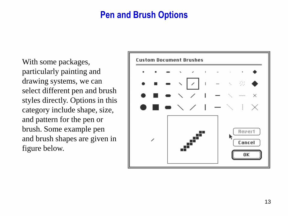
Pen and Brush Options
With some packages,
particularly painting and
drawing systems, we can
select different pen and brush
styles directly. Options in this
category include shape, size,
and pattern for the pen or
brush. Some example pen
and brush shapes are given in
figure below.

14
Line Style
By default, a straight-line segment is displayed as a solid line. However, we
can also display dashed lines, dotted lines, or a line with a combination of
dashes and dots, and we can vary the length of the dashes and the spacing
between dashes or dots. We set a current display style for lines with the
OpenGL function
glLineStipple (repeatFactor, pattern)
Parameter pattern is used to reference a 16-bit integer that describes how
the line should be displayed. A 1 bit in the pattern denotes an “on” pixel
position, and a 0 bit indicates an “off” pixel position. The pattern is applied
to the pixels along the line path starting with the low-order bits in the
pattern. The default pattern is 0xFFFF (each bit position has a value of 1),
which produces a solid line. Integer parameter repeatFactor specifies how
many times each bit in the pattern is to be repeated before the next bit in the
pattern is applied. The default repeat value is 1.
15
Line Style
•With a polyline, a specified line-style pattern is not restarted at the
beginning of each segment. It is applied continuously across all the
segments, starting at the first endpoint of the polyline and ending at the final
endpoint for the last segment in the series.
•As an example of specifying a line style, suppose that parameter pattern is
assigned the hexadecimal representation 0x00FF and the repeat factor is 1.
This would display a dashed line with eight pixels in each dash and eight
pixel positions that are “off” (an eight-pixel space) between two dashes.
Also, because low-order bits are applied first, a line begins with an eight-
pixel dash starting at the first endpoint. This dash is followed by an eight-
pixel space, then another eight-pixel dash, and so forth, until the second
endpoint position is reached.

16
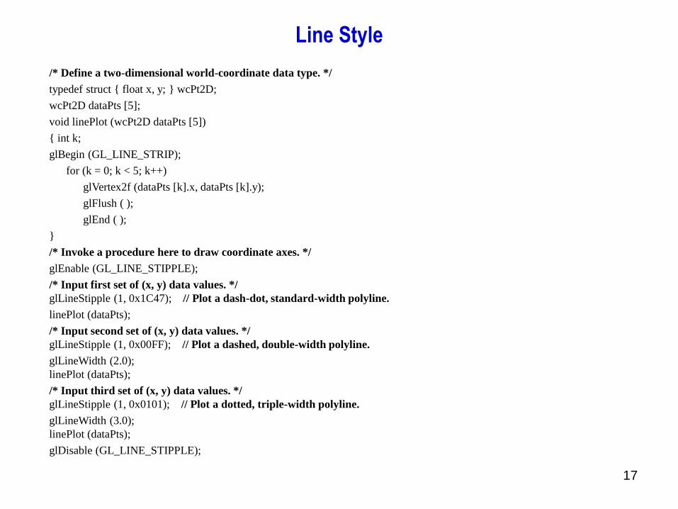
Line Style
•Before a line can be displayed in the current line-style pattern, we must
activate the line-style feature of OpenGL. We accomplish this with the
following function:
•glEnable (GL_LINE_STIPPLE); If we forget to include this enable
function, solid lines are displayed; that is, the default pattern 0xFFFF is used
to display line segments.
At any time, we can turn off the line-pattern feature with
•glDisable (GL_LINE_STIPPLE); This replaces the current line-style
pattern with the default pattern (solid lines).
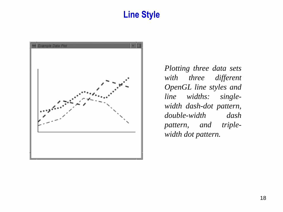
In the following program outline in the next slide, I’m showing the use of
the OpenGL line- attribute functions by plotting three line graphs in different
styles and widths.
17
Line Style
/* Define a two-dimensional world-coordinate data type. */
typedef struct { float x, y; } wcPt2D;
wcPt2D dataPts [5];
void linePlot (wcPt2D dataPts [5])
{ int k;
glBegin (GL_LINE_STRIP);
for (k = 0; k < 5; k++)
glVertex2f (dataPts [k].x, dataPts [k].y);
glFlush ( );
glEnd ( );
}
/* Invoke a procedure here to draw coordinate axes. */
glEnable (GL_LINE_STIPPLE);
/* Input first set of (x, y) data values. */
glLineStipple (1, 0x1C47); // Plot a dash-dot, standard-width polyline.
linePlot (dataPts);
/* Input second set of (x, y) data values. */
glLineStipple (1, 0x00FF); // Plot a dashed, double-width polyline.
glLineWidth (2.0);
linePlot (dataPts);
/* Input third set of (x, y) data values. */
glLineStipple (1, 0x0101); // Plot a dotted, triple-width polyline.
glLineWidth (3.0);
linePlot (dataPts);
glDisable (GL_LINE_STIPPLE);
18
Line Style
Plotting three data sets
with three different
OpenGL line styles and
line widths: single-
width dash-dot pattern,
double-width dash
pattern, and triple-
width dot pattern.

19
Line Style
Other OpenGL Line-Effects:
In addition to specifying width, style, and a solid color, we can display lines
with color gradations. For example, we can vary the color along the path of
a solid line by assigning a different color to each line endpoint as we define
the line. In the following code segment, we illustrate this by assigning a blue
color to one endpoint of a line and a red color to the other endpoint. The
solid line is then displayed as a linear interpolation of the colors at the two
endpoints:
glShadeModel (GL_SMOOTH);
glBegin (GL_LINES);
glColor3f (0.0, 0.0, 1.0);
glVertex2i (50, 50);
glColor3f (1.0, 0.0, 0.0);
glVertex2i (250, 250);
glEnd ( );

20
Line Style
Other OpenGL Line-Effects:
Function glShadeModel can also be given the argument GL FLAT. In that
case, the line segment would have been displayed in a single color: the color
of the second endpoint, (250, 250). That is, we would have generated a red
line. Actually, GL SMOOTH is the default, so we would generate a
smoothly interpolated color line segment even if we did not include this
function in our code.
We can produce other effects by displaying adjacent lines that have different
colors and patterns. In addition, we can use the color-blending features of
OpenGL by superimposing lines or other objects with varying alpha values.
A brush stroke and other painting effects can be simulated with a pixmap
and color blending. The pixmap can then be moved interactively to generate
line segments. Individual pixels in the pixmap can be assigned different
alpha values to display lines as brush or pen strokes.

21
Curve Attributes
❖ Parameters for curve attributes are the same as those for straight-line
segments.
❖ We can display curves with varying colors, widths, dot-dash patterns, and
available pen or brush options.
❖ Methods for adapting curve-drawing algorithms to accommodate attribute
selections are like those for line drawing.
❑ Methods for curve-drawing :
1) Curve Width
a) Using the method of horizontal or vertical pixel spans
b) Using fill area between the two parallel curve paths
2) Curve Style
a) Pixel masks methods
b) Pen (or brush ) methods

22
Strictly speaking, OpenGL does not consider curves to be drawing primitives in the
same way that it considers points and lines to be primitives. Curves can be drawn in
several ways in OpenGL. Perhaps the simplest approach is to approximate the shape
of the curve using short line segments. Alternatively ,curved segments can be drawn
using splines. These can be drawn using OpenGL evaluator functions, or by using
functions from the OpenGL Utility (GLU) library which draw splines.
Curve Width Methods
▪ Raster curves of various widths can be displayed using the method of horizontal
or vertical pixel spans.
▪ Where the magnitude of the curve slope is less than or equal to 1.0, we plot
vertical spans.
▪ where the slope magnitude is greater than 1.0, we plot horizontal spans.
Curve Attributes

23
A Circular arc of width 4 plotted with
either vertical or horizontal pixel spans,
depending on the slope .
Thich Curves
▪ Displaying thick curves is to fill in the area between two parallel curve path,
whose separation distance is equal to the desired width
A circular arc of width 4 and radius 16
displayed by filling the region between
two concentric arcs
Curve Attributes

24
Curve Attributes
Pixel patterns for curved path styles :
▪ pixel masks discussed for implementing line-style options could also be used in
raster curve algorithms to generate dashed or dotted patterns .
▪ For example, the mask 11100 produces the dashed circle shown in the Figure
A dashed circular arc displayed with a dash span of
3 pixels and an inter-dash spacing of 2 pixels

25
Curve Attributes
▪ Pen (or brush) displays of curves are generated using the same techniques
discussed for straight-line segments.
▪ We replicate a pen shape along the line path, as illustrated in the Figure
bellow for a circular arc in the first quadrant.
▪ Here, the center of the rectangular pen is moved to successive curve
positions to produce the curve shape shown.
A circular arc displayed with a rectangular
pen .
26
Curve Attributes
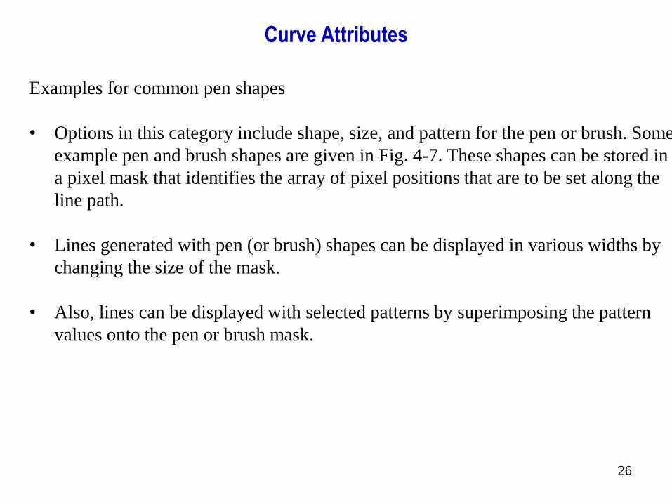
Examples for common pen shapes
• Options in this category include shape, size, and pattern for the pen or brush. Some
example pen and brush shapes are given in Fig. 4-7. These shapes can be stored in
a pixel mask that identifies the array of pixel positions that are to be set along the
line path.
• Lines generated with pen (or brush) shapes can be displayed in various widths by
changing the size of the mask.
• Also, lines can be displayed with selected patterns by superimposing the pattern
values onto the pen or brush mask.

27
a. Displayed by centering the mask over a specified pixel position.

28
Curve Attributes
Curve Patterns
▪ Different shapes and patterns may be used for curve drawing implementation,
shown in the figure below.
Curved lines drawn with a paint program using various shapes and
patterns . From left to right, the brush shapes are square, round,
diagonal line, dot pattern, and faded airbrush.
29
Fill-Area Attributes
• we can fill any specified regions, including circles, ellipses, and other objects with
curved boundaries. And applications systems, such as paint programs, provide fill
options for arbitrarily shaped region.
• . The scan-line approach is usually applied to simple shapes such as circles or
regions with polyline boundaries, and general graphics packages use this fill
method.
• Fill algorithms that use a starting interior point are useful for filling areas with
more complex boundaries and in interactive painting systems
• There are two basic procedures for filling an area on raster systems, once the
definition of the fill region has been mapped to pixel coordinates:
a) One procedure first determines the overlap intervals for scan lines that cross the area.
Then, pixel positions along these overlap intervals are set to the fill color.
b) Another method for area filling is to start from a given interior position and “paint”
outward, pixel by-pixel, from this point until we encounter specified boundary conditions.

30
Enabling polygon fill (Default):
glPolygonMode(GL_FRONT_AND_BACK, GL_FILL);
Disabling polygon fill:
glPolygonMode(GL_FRONT_AND_BACK, GL_LINE);
Fill-Area Attributes
• glPolygonMode controls the interpretation of polygons for rasterization. face
describes which polygons mode applies to both front and back-facing polygons
(GL_FRONT_AND_BACK).
• The polygon mode affects only the final rasterization of polygons.
• In particular, a polygon's vertices are lit, and the polygon is clipped and possibly
culled before these modes are applied

31
Fill-Area Attributes
▪ Fill Styles :
a. Hollow : Only the boundary is displayed
b. Solid : of desired color
c. Patterned : different colors and shapes
32
Fill-Area Attributes
▪ Fill patterns can be defined in:
• Rectangular color arrays that list different colors for different positions
in the array.
• Or, In a fill pattern could be specified as a bit array that indicates which
relative positions are to be displayed in a single selected color.
• Other fill patterns:
• Using array masks
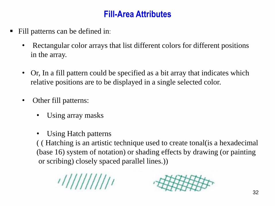
• Using Hatch patterns
( ( Hatching is an artistic technique used to create tonal(is a hexadecimal
(base 16) system of notation) or shading effects by drawing (or painting
or scribing) closely spaced parallel lines.))

33
Fill-Area Attributes
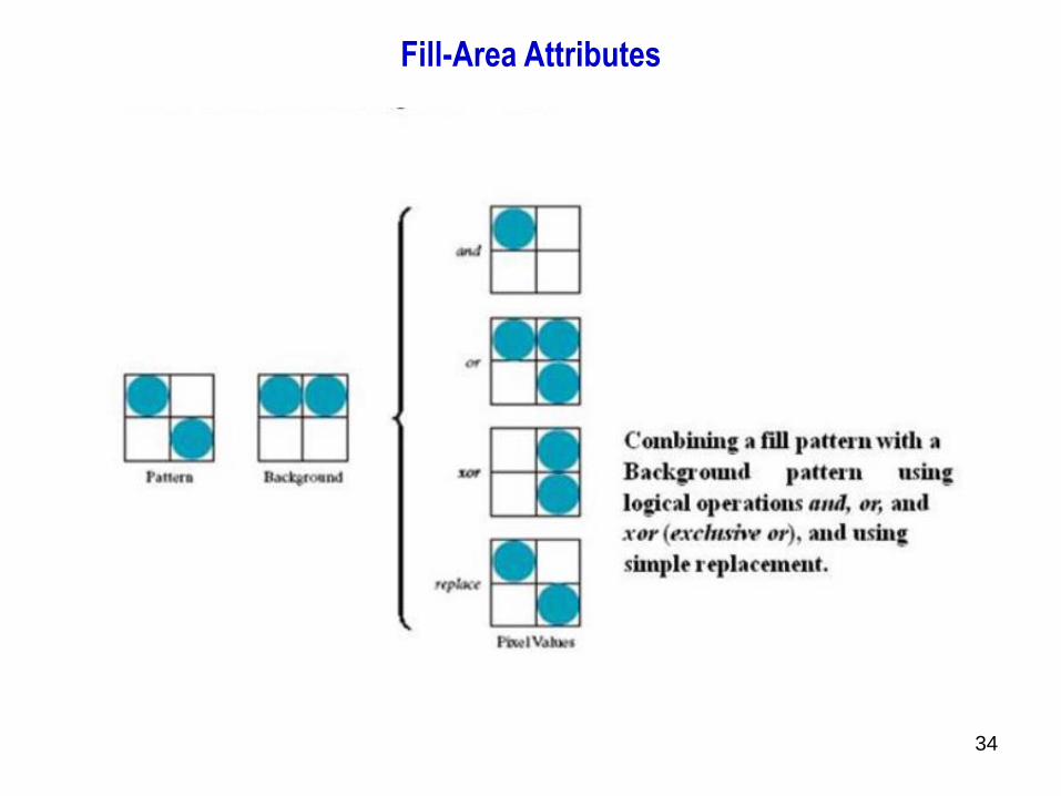
Area fill with logical operators / Color – Blended Fill Regions
• A pattern could be combined with background colors using a transparency
factor that determines how much of the background should be mixed with the
object color.
• Or we could use simple logical or replace operations.
• Some fill methods using blended colors have been referred to as soft-fill
algorithm or tint-fill algorithm.
• One use for these fill methods is to allow repainting of a color area that was
originally filled with a semitransparent brush, where the current color is then a
mixture of the brush color and the background colors “behind” the area.
• In either case, we want the new fill color to have the same variations over the
area as the current fill color.
34
Fill-Area Attributes

35
Fill-Area Attributes
OpenGL FILL-AREA ATTRIBUTE FUNCTIONS
We generate displays of filled convex polygons in four steps:
(1) Define a fill pattern.
(2) Invoke the polygon-fill routine.
(3) Activate the polygon-fill feature of OpenGL.
(4) Describe the polygons to be filled.

36
Fill-Area Attributes
OpenGL Fill-Pattern Function:
OpenGL Fill-Pattern Function A convex polygon is displayed as a solid-color
region, using the current color setting.
To fill the polygon with a pattern in OpenGL, we use a 32-bit by 32- bit mask.
The fill pattern is specified in unsigned bytes using the OpenGL data type GLubyte,
just as we did with the glBitmap function
This pattern is replicated across the entire area of the display window, starting at the
lower-left window corner, and specified polygons are filled where the pattern
overlaps those polygons.
Once we have set a mask, we can establish it as the current fill pattern with the
function glPolygonStipple (fillPattern);
Next, we need to enable the fill routines before we specify the vertices for the
polygons that are to be filled with the current pattern.
We do this with the statement
glEnable (GL_POLYGON_STIPPLE);

37
Fill-Area Attributes
OpenGL Texture and Interpolation Patterns:
OpenGL Texture and Interpolation Patterns This can produce fill patterns that simulate the surface
appearance of wood, brick, brushed steel, or some other material.
Also, we can obtain an interpolation coloring of a polygon interior just as we did with the line primitive.
The polygon fill is then a linear interpolation of the colors at the vertices.
glShadeModel (GL_SMOOTH);
glBegin (GL_TRIANGLES);
glColor3f (0.0, 0.0, 1.0)
glVertex2i (50, 50)
glColor3f (1.0, 0.0, 0.0);
glVertex2i (150, 50);
glColor3f (0.0, 1.0, 0.0);
glVertex2i (75, 150)
glEnd ( );
If we change the argument in the glShadeModel function to GL FLAT in this example, the polygon is filled
with the last color specified (green).
The value GL SMOOTH is the default shading, but we can include that specification to remind us that the
polygon is to be filled as an interpolation of the vertex colors.
38
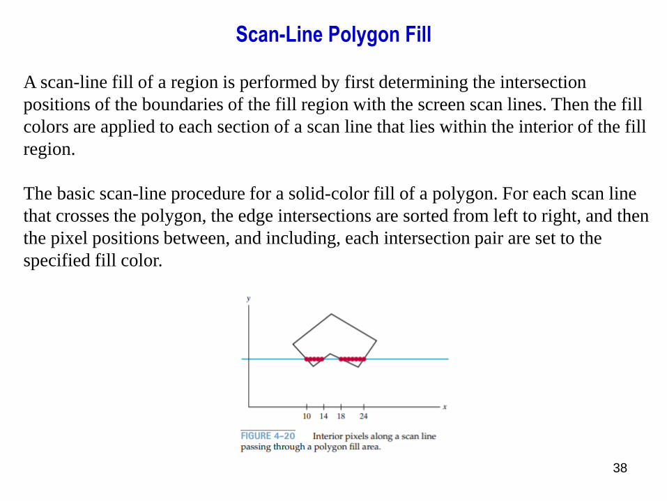
Scan-Line Polygon Fill
A scan-line fill of a region is performed by first determining the intersection
positions of the boundaries of the fill region with the screen scan lines. Then the fill
colors are applied to each section of a scan line that lies within the interior of the fill
region.
The basic scan-line procedure for a solid-color fill of a polygon. For each scan line
that crosses the polygon, the edge intersections are sorted from left to right, and then
the pixel positions between, and including, each intersection pair are set to the
specified fill color.

39
Scan-Line Polygon Fill
One method for implementing the adjustment to the vertex-intersection count is to
shorten some polygon edges to split those vertices that should be counted as one
intersection.
We can process nonhorizontal edges around the polygon boundary in the order
specified, either clockwise or counterclockwise.
As we process each edge, we can check to determine whether that edge and the
next nonhorizontal edge have either monotonically increasing or decreasing
endpoint y values.
40
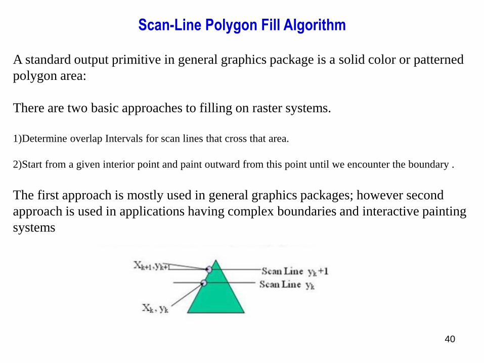
Scan-Line Polygon Fill Algorithm
A standard output primitive in general graphics package is a solid color or patterned
polygon area:
There are two basic approaches to filling on raster systems.
1)Determine overlap Intervals for scan lines that cross that area.
2)Start from a given interior point and paint outward from this point until we encounter the boundary .
The first approach is mostly used in general graphics packages; however second
approach is used in applications having complex boundaries and interactive painting
systems
41
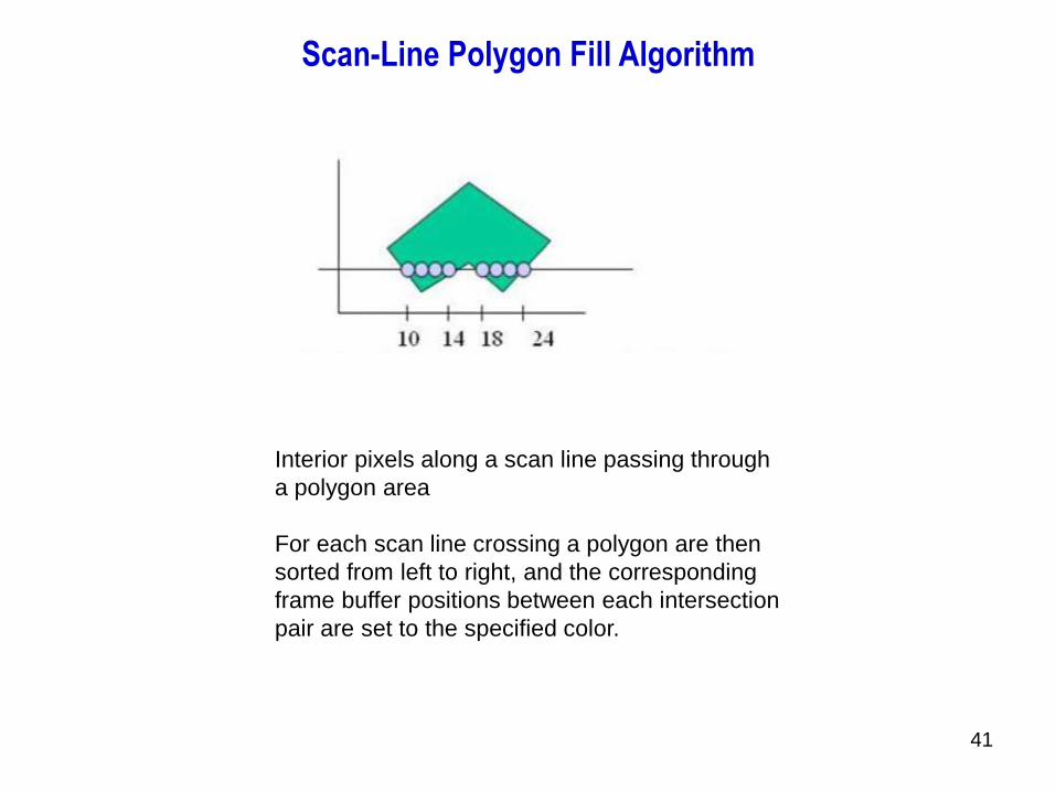
Scan-Line Polygon Fill Algorithm
Interior pixels along a scan line passing through
a polygon area
For each scan line crossing a polygon are then
sorted from left to right, and the corresponding
frame buffer positions between each intersection
pair are set to the specified color.
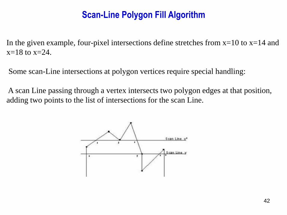
42
In the given example, four-pixel intersections define stretches from x=10 to x=14 and
x=18 to x=24.
Some scan-Line intersections at polygon vertices require special handling:
A scan Line passing through a vertex intersects two polygon edges at that position,
adding two points to the list of intersections for the scan Line.
Scan-Line Polygon Fill Algorithm

43
Scan-Line Polygon Fill Algorithm
One way to resolve this is also to shorten some polygon edges to split those vertices
that should be counted as one intersection.
When the end point y coordinates of the two edges are increasing , the y value of
the upper endpoint for the current edge is decreased by 1 .
When the endpoint y values are decreasing, we decrease the y coordinate of the
upper endpoint of the edge following the current edge.

44
In determining fill-area edge intersections, we can set up incremental coordinate
calculations along any edge by exploiting the fact that the slope of the edge is
constant from one scan line to the next. Figure shows two successive scan lines
crossing the left edge of a triangle.
The slope of this edge can be expressed in terms of the scan-line intersection
coordinates:
Mathematical Model

45
Since the change in y coordinates between the two scan lines is simply
The x-intersection value xk+1 on the upper scan line can be determined from the
x-intersection value xk on the preceding scan line as
Each successive x intercept can thus be calculated by adding the inverse of the
slope and rounding to the nearest integer.
46
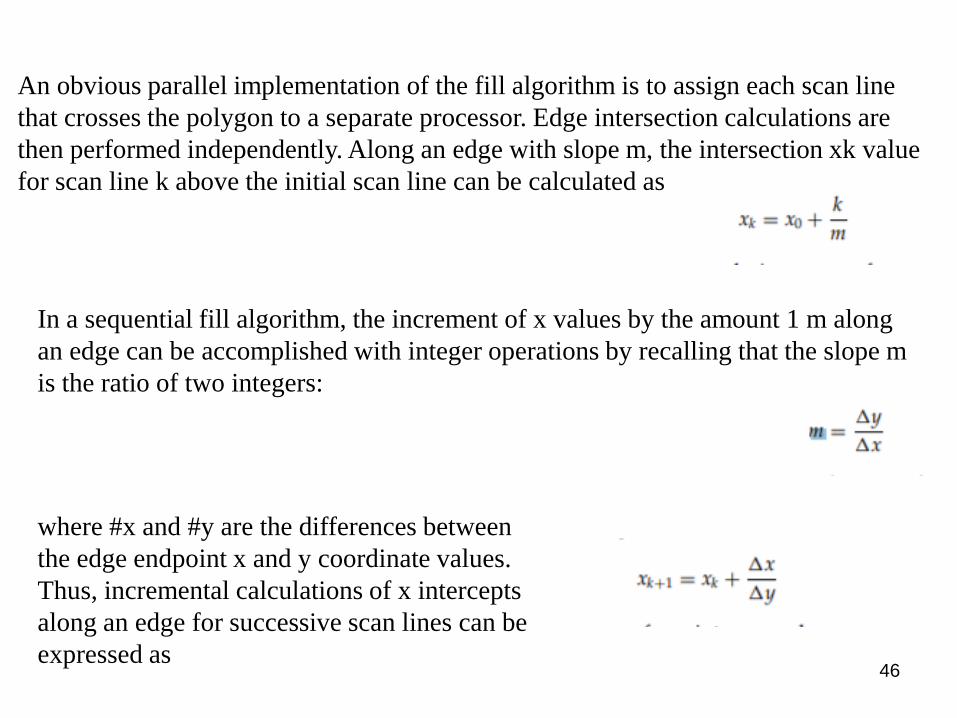
An obvious parallel implementation of the fill algorithm is to assign each scan line
that crosses the polygon to a separate processor. Edge intersection calculations are
then performed independently. Along an edge with slope m, the intersection xk value
for scan line k above the initial scan line can be calculated as
In a sequential fill algorithm, the increment of x values by the amount 1 m along
an edge can be accomplished with integer operations by recalling that the slope m
is the ratio of two integers:
where #x and #y are the differences between
the edge endpoint x and y coordinate values.
Thus, incremental calculations of x intercepts
along an edge for successive scan lines can be
expressed as

47
To efficiently perform a polygon fill, we can first store the polygon boundary in a
sorted edge table that contains all the information necessary to process the scan
lines efficiently.
Proceeding around the edges in either a clockwise or a counterclockwise order,
we can use a bucket sort to store the edges, sorted on the smallest y value of each
edge, in the correct scan-line positions.
Only nonhorizontal edges are entered into the sorted edge table. As the edges are
processed, we can also shorten certain edges to resolve the vertex-intersection
question.
Next, we process the scan lines from the bottom of the polygon to its top, producing
an active edge list for each scan line crossing the polygon boundaries.
The active edge list for a scan line contains all edges crossed by that scan line, with
iterative coherence calculations used to obtain the edge intersections
Global edge list and active edge list

48

49
Scan-Line Fill Methods
If the boundary of some region is specified in a single color, we can fill the interior
of this region, pixel by pixel, until the boundary color is encountered.
This method called the boundary-fill algorithm, where interior points are easily
selected. The figure interior is then painted in the fill color.
Both inner and outer boundaries can be set up to define an area for boundary fill, a
boundary-fill algorithm starts from an interior point ( x, y) and tests the color of
neighboring positions.
If a tested position is not displayed in the boundary color, its color is changed to the
fill color and its neighbors are tested.

50
Scan-Line Fill Methods
4-connected
This procedure continues until all pixels are processed up to the designated boundary
color for the area. Areas filled by this method are called 4-connected.
8-connected
Here the set of neighboring positions to be tested includes the four diagonal pixels,
as well as those in the cardinal directions.
Fill methods using this approach are called 8-connected.
An 8-connected boundary-fill algorithm would correctly fill the interior of the area
,but a 4-connected boundary-fill algorithm would only fill part of that region.

51
Scan-Line Fill Methods
Pseudo Code
52
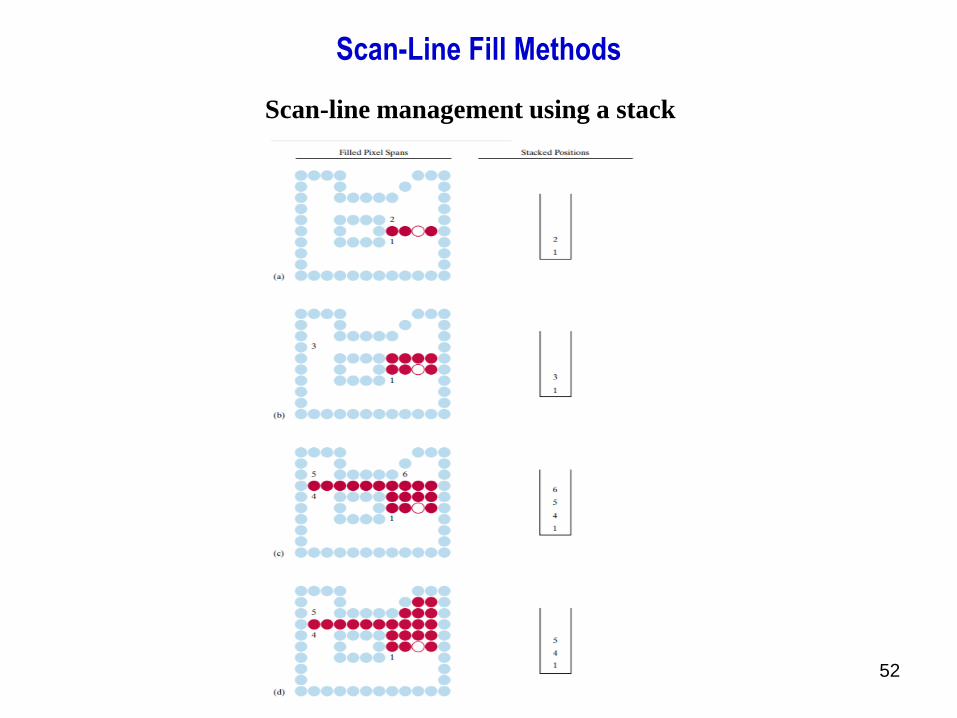
Scan-Line Fill Methods
Scan-line management using a stack
53
Wire-Frame Methods
We can also choose to show only polygon edges. This produces a wire-frame or
hollow display of the polygon. Or we could display a polygon by only plotting a set
of points at the vertex positions.
These options are selected with the function glPolygonMode (face, displayMode);
We use parameter face to designate which face of the polygon we want to show as
edges only or vertices only. This parameter is then assigned either GL FRONT, GL
BACK, or GL FRONT AND BACK
Then, if we want only the polygon edges displayed for our selection, we assign the
constant GL LINE to parameter display Mode.).
To plot only the polygon vertex points, we assign the constant GL POINT to
parameter displayMode.

54
Wire-Frame Methods
A third option is GL FILL. But this is the default display mode, so we usually only
invoke glPolygonMode when we want to set attributes for the polygon edges or
vertices.
Another option is to display a polygon with both an interior fill and a different color
or pattern for its edges (or for its vertices).
This is accomplished by specifying the polygon twice: once with parameter
displayMode set to GL FILL and then again with displayMode set to GL LINE (or
GL POINT).
For a three-dimensional polygon (one that does not have all vertices in the xy
plane), this method for displaying the edges of a filled polygon may produce gaps
along the edges. This effect, sometimes referred to as stitching, is caused by
differences between calculations in the scan-line fill algorithm and calculations in
the edge line-drawing algorithm

55
Wire-Frame Methods
One way to eliminate the gaps along displayed edges of a three-dimensional polygon
is to shift the depth values calculated by the fill routine so that they do not overlap
with the edge depth values for that polygon. We do this with the following two
OpenGL functions.
glEnable (GL_POLYGON_OFFSET_FILL);
glPolygonOffset (factor1, factor2);
The first function activates the offset routine for scan-line filling.
The second function is used to set a couple of floating-point values factor1 and
factor2 that are used to calculate the amount of depth offset.
The calculation for this depth offset is
depthOffset = factor1 · maxSlope + factor2 · const
MaxSlope is the maximum slope of the polygon and const is an implementation
constant

56
OpenGL Front-Face Function
Although, by default, the ordering of polygon vertices controls the identification of
front and back faces, we can independently label selected surfaces in a scene as front
or back with the function glFrontFace (vertexOrder);
If we set parameter vertexOrder to the OpenGL constant GL CW, then a
subsequently defined polygon with a clockwise ordering for its vertices is Character
Attributes 211 to be front facing.
This OpenGL feature can be used to swap faces of a polygon for which we have
specified vertices in a clockwise order.
The constant GL CCW labels a counterclockwise ordering of polygon vertices as
front facing, which is the default ordering
Wire-Frame Methods
57
Character Attributes
We control the appearance of displayed characters with attributes such as font,
size, color, and orientation. In many packages, attributes can be set both for
entire character strings (text) and for individual characters that can be used for
special purposes such as plotting a data graph.
There is the choice of font (or typeface), which is a set of characters with a
particular design style such as New York, Courier, Helvetica, London, Times
Roman, and various special symbol groups. The characters in a selected font can
also be displayed with assorted underlining styles (solid, ------- dotted, double), in
boldface, in italics, and in OUTLINE or shadow styles.
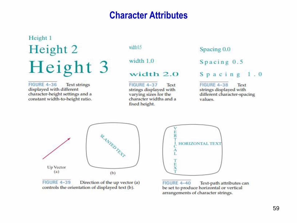
We could adjust text size by scaling the overall dimensions (height and width) of
characters or by scaling only the height or the width.
Character size (height) is specified by printers and compositors in points,
where1point is about 0.035146 centimeters (or 0.013837 inch, which is
approximately 1 72 inch).

58
Character Attributes
Point measurements specify the size of the body of a character , but different fonts
with the same point specifications can have different character sizes, depending on the
design of the typeface.
The distance between the bottomline and the topline of the character body is the same
for all characters in a particular size and typeface, but the body width may vary.
Character height is defined as the distance between the baseline and the capline of
characters
Spacing between characters is another attribute that can often be assigned to a
character string
59
Character Attributes

60
Character Attributes
61
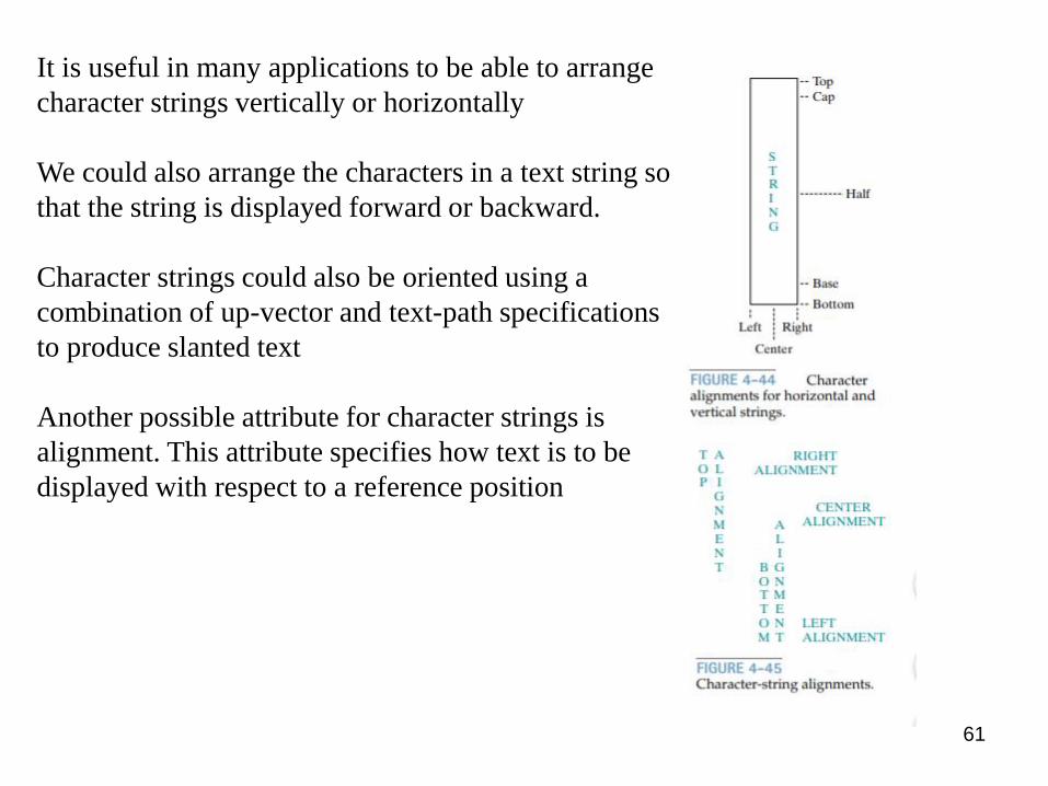
It is useful in many applications to be able to arrange
character strings vertically or horizontally
We could also arrange the characters in a text string so
that the string is displayed forward or backward.
Character strings could also be oriented using a
combination of up-vector and text-path specifications
to produce slanted text
Another possible attribute for character strings is
alignment. This attribute specifies how text is to be
displayed with respect to a reference position

62
Character Attributes
We have two methods for displaying characters with the OpenGL package. Either
we can design a font set using the bitmap functions in the core library, or we can
invoke the GLUT character-generation routines.
In general, the spacing and size of characters is determined by the font
designation, such as GLUT BITMAP 9 BY 15 and GLUT STROKE MONO
ROMAN.
We specify the width for a line with the glLineWidth function, and we select a
line type with the glLineStipple function
The transformation routines allow us to scale, position, and rotate the GLUT
stroke characters in either two-dimensional space or three-dimensional space. In
addition, the three-dimensional viewing transformations can be used to generate
other display effects.
OpenGl Character-Attribute Functions

63
Anti-aliasing
Intensity signal along a scan-line:
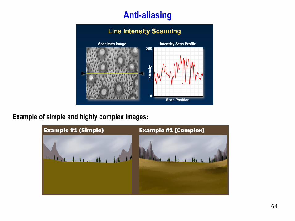
The line intensity scan function is a graphical tool that is useful for measuring intensity and
contrast along a single horizontal or vertical row of pixels in digital images. This technique is
often employed to compare brightness values in related digital images, and to determine the
average values over several adjacent pixel rows in a single image.
The line intensity scan function consists of a graph of pixel intensity values measured at each
position along a horizontal (or vertical) scan line through a digital image. Relative height
differences between points on the graph correspond to brightness differences between objects
in the image. By comparing the height differences of various points on the graph, useful
information regarding local and global image contrast can be obtained.
For a color digital image, a line intensity scan of the red, green, and blue color channels can
be produced when the image is stored in the RGB color model. Similarly, a line intensity
scan of an image can also be produced when it is stored in
the HSI (Hue, Saturation, Intensity) color model.
64
Anti-aliasing
Example of simple and highly complex images:
65
Anti-aliasing
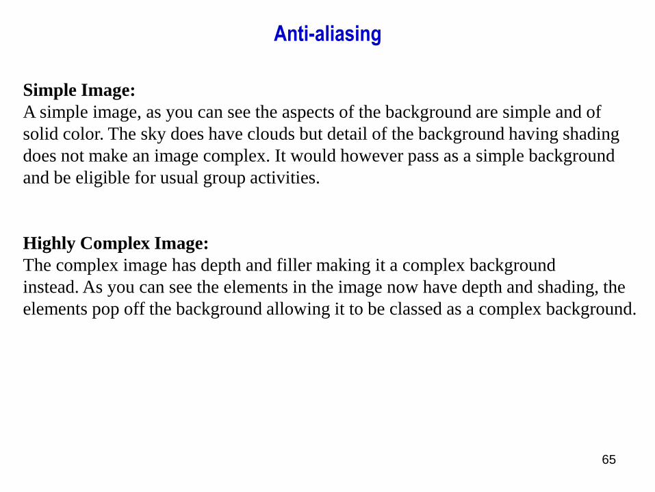
Simple Image:
A simple image, as you can see the aspects of the background are simple and of
solid color. The sky does have clouds but detail of the background having shading
does not make an image complex. It would however pass as a simple background
and be eligible for usual group activities.
Highly Complex Image:
The complex image has depth and filler making it a complex background
instead. As you can see the elements in the image now have depth and shading, the
elements pop off the background allowing it to be classed as a complex background.

66
Anti-aliasing
Sampling an Image:
An image may be continuous w.r.t x and y co-ordinate and also in amplitude. To
convert it to digital form, we have to sample the function in both co-ordinate and
amplitude.
Sampling :
The process of digitizing the co-ordinate values is called Sampling.
A continuous image f(x, y) is normally approximated by equally spaced samples
arranged in the form of a NxM array where each elements of the array is a discrete
quantity.
The sampling rate of digitizer determines the spatial resolution of digitized image.
Finer the sampling (i.e. increasing M and N), the better the approximation of
continuous image function f(x, y).

67
Anti-aliasing
Take enough samples to allow reconstructing the “continuous” image from its
samples.
Types:
1. Up sampling / Over sampling
2. Down sampling
The increase in the quantity of pixels is done through oversampling.
68
Anti-aliasing
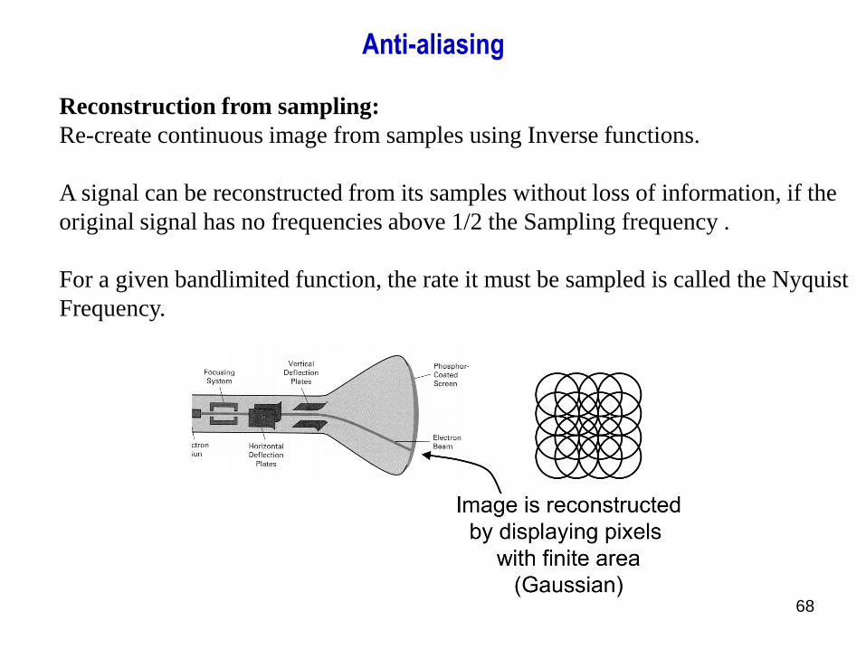
Reconstruction from sampling:
Re-create continuous image from samples using Inverse functions.
A signal can be reconstructed from its samples without loss of information, if the
original signal has no frequencies above 1/2 the Sampling frequency .
For a given bandlimited function, the rate it must be sampled is called the Nyquist
Frequency.

69
Anti-aliasing
Sampling challenges: too few points and slivers:
1. Band-limited functions have infinite duration in the time domain.
But, we can only sample a function over a finite interval.
•We would need to obtain a finite set of samples by multiplying with a “box”
function:
[s(x)f(x)] h(x)
x =

70
Anti-aliasing
Anti-aliasing and Resolution:Because display resolution is intrinsically linked with spatial anti-aliasing, one needs to know
a little bit about their relationship to gain a full understanding of how it all works. Display
resolution is essentially the number of pixels used by your monitor when creating the image
you will see on the screen. Standard monitors will have minimum display resolutions of 1920
x 1080. This equates to 1920 pixels being used for the screen’s X-axis and 1080 on the Y-
axis.
Anti-aliasing (spatial):
You have an image that’s being seen at a low resolution, and this results in jaggies.
With spatial anti-aliasing, the image will be rendered at a resolution higher than the one set.
Excess pixels produced by this higher resolution will be used as color samples.
This image is reduced back to its original resolution, but every pixel that it has will receive
new colors that have been averaged using the color samples.
In summary, low-resolution images will get the same color accuracy as their high-resolution
counterparts. These optimized colors will help each pixel blend with each other more
smoothly, resulting in less visible jaggies.

71
Anti-aliasing
Stair casing effect due to low resolution:
Jaggies is the informal name for artifacts in raster images, most frequently from
aliasing, which in turn is often caused by non-linear mixing effects producing high-
frequency components, or missing or poor anti-aliasing filtering prior to sampling.
Jaggies are stair-like lines that appear where there should be "smooth" straight lines
or curves. For example, when a nominally straight, un-aliased line steps across one
pixel either horizontally or vertically, a "dogleg" occurs halfway through the line,
where it crosses the threshold from one pixel to the other.
Jaggies occur due to the "staircase effect". This is because a line represented in
raster mode is approximated by a sequence of pixels. Jaggies can occur for a variety
of reasons, the most common being that the output device (display monitor or
printer) does not have enough resolution to portray a smooth line. In addition,
jaggies often occur when a bit-mapped image is converted to a different resolution.
This is one of the advantages that vector graphics have over bitmapped graphics –
the output looks the same regardless of the resolution of the output device.

72
Anti-aliasingContent outline:
• Stair casing effect due to low resolution
• Edge smoothing using blurring
Jaggies occur due to the "staircase effect". This is because a line represented in
raster mode is approximated by a sequence of pixels. Jaggies can occur for a variety
of reasons, the most common being that the output device (display monitor or
printer) does not have enough resolution to portray a smooth line. In addition,
jaggies often occur when a bit-mapped image is converted to a different resolution.
This is one of the advantages that vector graphics have over bitmapped graphics –
the output looks the same regardless of the resolution of the output device.

73
Anti-aliasing
Edge smoothing using blurring:
Blurring is a technique in digital image processing in which we perform a
convolution operation between the given image and a predefined low-pass filter
kernel. The image looks sharper or more detailed if we are able to perceive all the
objects and their shapes correctly in it. E.g. An image with a face looks clearer
when we can identify eyes, ears, nose, lips, forehead, etc. very clear. This shape
of the object is due to its edges. So, in blurring, we simply reduce the edge
content and makes the transition from one color to the other very smooth. It is
useful for removing noise.
Types of filters in Blurring:
When smoothing or blurring images, we can use diverse linear(Spatial) filters,
because linear filters are easy to achieve, and are kind of fast, the most used ones
are Homogeneous filter, Gaussian filter, Median filter. However, there are few
non-linear filters like a bilateral filter, an adaptive bilateral filter, etc that can be
used where we want to blur the image while preserving its edges.

74
Anti-aliasing
Signal reconstruction based on sampling:
The process of reconstructing a continuous time signal x(t) from its samples is known
as interpolation. In the sampling theorem we saw that a signal x(t) band limited to D Hz can be
reconstructed from its samples. This reconstruction is accomplished by passing the sampled signal
through an ideal low pass filter of bandwidth D Hz. The sampled signal contains a component
and to recover x(t) or X(f), the sampled signal must be passed through an ideal lowpass filter having
bandwidth D Hz and gain T. The description of the process of reconstruction in the frequency domain
is to find the DTFT of the discrete-time signal, change the variable F tends to f / fs , multiply by T and
find the inverse CTFT. We find the DTFT from the samples using
Interpolation consists of simply of multiplying each sinc function by its corresponding sample value
and then adding all the scaled and shifted sinc functions.

75
Anti-aliasing
Minimum frequency:
1. There is a minimum frequency with which functions must be sampled – the Nyquist
frequency.
Twice the maximum frequency present in the signal.
2. Signals that are not bandlimited cannot be accurately sampled and reconstructed
3. Not all sampling schemes allow reconstruction
eg: Sampling with a box
Poor reconstruction also results in aliasing.

76
Anti-aliasing
Pixel super-sampling:
In computer graphics, supersampling is the process of sampling an image at a frequency
higher than the target sampling frequency (usually the pixel frequency). The key idea of
supersampling is the same as the one in oversampling. However, in supersampling, no
analog filtering or quantization is involved.
Supersampling, when combined with filtered decimation (reducing the sampling
frequency by 'averaging down'), is a simple and effective method for anti-aliasing when
prefiltering (filtering the continuous signal before any sampling) is difficult or impossible.
Aliasing is a pervasive problem in computer graphics. The sharp edges in computer
graphics models represent arbitrarily large frequencies. Furthermore, prefiltering in
rendering applications is very difficult. Supersampling is a simple and effective alternative
in these cases.

77
Anti-aliasing
Weighted pixel distribution:
Pixels are processed on the image based on different attributes such as mean, average of
colors at each pixel. This is used in filters.
A bilateral filter is a non-linear, edge-preserving, and noise-reducing smoothing filter for
images. It replaces the intensity of each pixel with a weighted average of intensity values
from nearby pixels. This weight can be based on a Gaussian distribution. Crucially, the
weights depend not only on Euclidean distance of pixels, but also on the radiometric
differences (e.g., range differences, such as color intensity, depth distance, etc.). This
preserves sharp edges.
78
Anti-aliasing
Pixel intensity distribution based on area coverage:
An alternative to supersampling is to determine pixel intensity by calculating the areas of
overlap of each pixel with the objects to be displayed. Antialiasing by computing overlap
areas is referred to as area sampling (or prefiltering, because the intensity of the pixel as a
whole is determined without calculating subpixel intensities). Pixel overlap areas are
obtained by determining where object boundaries intersect individual pixel boundaries.
Raster objects can also be antialiased by shifting the display location of pixel areas. This
technique, called pixel phasing, is applied by “micropositioning” the electron beam in
relation to object geometry. For example, pixel positions along a straight-line segment can
be moved closer to the defined line path to smooth out the raster stair-step effect.
Filters:
A more accurate method for antialiasing lines is to use filtering techniques. The method is
similar to applying a weighted pixel mask, but now we imagine a continuous weighting
surface (or filter function) covering the pixel. Figure shows examples of rectangular,
conical, and Gaussian filter functions. Methods for applying the filter function are similar
to those for applying a weighting mask, but now we integrate over the pixel surface to
obtain the weighted average intensity. To reduce computation, table lookups are
commonly used to evaluate the integrals.

79
Anti-aliasing

80
Anti-aliasing
Methods of Antialiasing (AA) – Aliasing is removed using four methods:
Using high-resolution display, Post filtering (Supersampling), Pre-filtering
(Area Sampling), Pixel phasing.
Pixel phasing:
It’s a technique to remove aliasing. Here pixel positions are shifted to
nearly approximate positions near object geometry. Some systems allow
the size of individual pixels to be adjusted for distributing intensities
which is helpful in pixel phasing.

81
Anti-aliasing
Subpixel computation:
Antialiasing of edges is often performed with the help of subpixel masks that
indicate which parts of the pixel are covered by the object that has to be
drawn. For this purpose, subpixel masks have to be generated during the scan
conversion of an image. Sub-pixel rendering requires special colour-balanced
anti-aliasing filters to turn what would be severe colour distortion into barely-
noticeable colour fringes.
Figure : Number of set subpixels vs. area covered. a) Result of supersampling with a horizontal or vertical line, b) Supersampling with a diagonal line, c) Ideal function.

82
Anti-aliasing
An ideal anti-alias filter passes all the appropriate input frequencies (below f1) and
cuts off all the undesired frequencies (above f1). However, such a filter is not
physically realizable. In practice, filters look as shown in illustration (b) below. They
pass all frequencies < f1, and cut-off all frequencies > f2. The region
between f1 and f2 is known as the transition band, which contains a gradual
attenuation of the input frequencies. Although you want to pass only signals with
frequencies < f1, those signals in the transition band could still cause aliasing.
Therefore in practice, the sampling frequency should be greater than two times the
highest frequency in the transition band. This turns out to be more than two times
the maximum input frequency (f1). That is one reason why you may see that the
sampling rate is more than twice the maximum input frequency.
83
References
• Computer Graphics with OpenGL D. Hearn, M. P. Baker and W. R. Carithers
Prentice Hall
• https://www.olympus-lifescience.com/en/microscope-
resource/primer/java/digitalimaging/processing/lineintensityscan

84
Thank you