introduction to braided geometry and -minkowski space · introduction to braided geometry and...
TRANSCRIPT

arX
iv:h
ep-t
h/94
1024
1v3
6 N
ov 1
994
Introduction to Braided Geometry and q-Minkowski Space
S. Majid1
Department of Applied Mathematics & Theoretical Physics, University of Cambridge, CambridgeCB3 9EW, UK
Abstract We present a systematic introduction to the geometry of linear braided spaces. Theseare versions of Rn in which the coordinates xi have braid-statistics described by an R-matrix.From this starting point we survey the author’s braided-approach to q-deformation: braideddifferentiation, exponentials, Gaussians, integration and forms, i.e. the basic ingredients forq-deformed physics are covered. The braided approach includes natural q-Euclidean and q-Minkowski spaces in R-matrix form.
Keywords: quantum groups – noncommutative geometry – braided geometry – q-Minkowski –q-Euclidean
Contents
1 Introduction 2
1.1 Why q-deform? . . . . . . . . . . . . . . . . . . . . . . . . . . . . . . . . . . . . . 21.2 What is braided geometry? . . . . . . . . . . . . . . . . . . . . . . . . . . . . . . 3
2 Diagrammatic definition of a braided group 4
3 Braided coaddition 7
3.1 Braided coaddition on vectors and covectors . . . . . . . . . . . . . . . . . . . . . 73.2 Braided coaddition on matrices A(R) and A(R) . . . . . . . . . . . . . . . . . . . 113.3 Braided coaddition on matrices B(R) . . . . . . . . . . . . . . . . . . . . . . . . . 14
4 Braided linear algebra 18
4.1 Braided linear transformations . . . . . . . . . . . . . . . . . . . . . . . . . . . . 184.2 Gluing or direct sum of braided vectors . . . . . . . . . . . . . . . . . . . . . . . 214.3 Braided metric . . . . . . . . . . . . . . . . . . . . . . . . . . . . . . . . . . . . . 254.4 Braided ∗-structures . . . . . . . . . . . . . . . . . . . . . . . . . . . . . . . . . . 26
5 Braided analysis 29
5.1 Braided differentiation . . . . . . . . . . . . . . . . . . . . . . . . . . . . . . . . . 295.2 Braided binomial theorem . . . . . . . . . . . . . . . . . . . . . . . . . . . . . . . 315.3 Duality of braided vectors and covectors . . . . . . . . . . . . . . . . . . . . . . . 335.4 Braided exponentials . . . . . . . . . . . . . . . . . . . . . . . . . . . . . . . . . . 345.5 Braided Gaussians . . . . . . . . . . . . . . . . . . . . . . . . . . . . . . . . . . . 375.6 Braided integration . . . . . . . . . . . . . . . . . . . . . . . . . . . . . . . . . . . 385.7 Braided electromagnetism . . . . . . . . . . . . . . . . . . . . . . . . . . . . . . . 39
6 Covariance 42
6.1 Induced braiding . . . . . . . . . . . . . . . . . . . . . . . . . . . . . . . . . . . . 446.2 Induced Poincare group . . . . . . . . . . . . . . . . . . . . . . . . . . . . . . . . 46
1Royal Society University Research Fellow and Fellow of Pembroke College, Cambridge. This paper is in final
form and no version of it will be submitted for publication elsewhere
1

7 q-Deformed spacetime 49
7.1 q-Euclidean space . . . . . . . . . . . . . . . . . . . . . . . . . . . . . . . . . . . . 497.2 q-Minkowski space . . . . . . . . . . . . . . . . . . . . . . . . . . . . . . . . . . . 51
A Transmutation 54
1 Introduction
It is often thought that quantum groups provide the key to q-deforming the basic structuresof physics from the point of view of non-commutative geometry. If one considered a classicalalgebra of observables and quantised it relative to some Poisson bracket, one might obtain aquantum group. The underlying semiclassical theory is the theory of Poisson-Lie groups – seeReyman’s lectures and Reshetikhin’s lectures on classical inverse scattering. But this is onlypart of the story. Our goal in these lectures is to explain that the fundamental concept neededfor the full structure of even the simplest q-deformed spaces, such as the quantum plane, is notso much a quantum group as one of the more exotic objects called braided groups. These wereintroduced by the author in 1989[1] and subsequently developed in the course of 40 or so papersinto a systematic theory of braided geometry. Quantum groups play a background role in thistheory as the quantum symmetry or covariance of the geometry, but the spaces themselves tendto be braided ones.
My intention is to provide here a pedagogical introduction to this theory of braided geometry.Braided groups provide a new beginning for the theory of q-deformation and can be developedalong-side quantum groups without requiring much experience of them. Instead, some experiencewith Grassmann algebras or supersymmetry will be quite helpful although not essential. We tryto cover here only q-deformed or braided versions of Rn, where the theory is fairly complete. Thisincludes important examples such as q-Euclidean and q-Minkowski space. Only when this lineartheory is thoroughly understood could one reasonably expect to move on to define q-manifoldsetc. For some first steps in quantum geometry, see [2]. Braided Yang-Mills theory on a generalbraided manifold is not yet understood.
We begin with the concept itself of a braided group. This is a new concept. On the onehand we replace old ideas form the theory of superspaces by similar ones with braid statistics inplace of Bose-Fermi ones. This makes it easy for the reader to get the idea of braided groups.On the other hand the true meaning and abstract definition of braided groups involves writingits algebraic structure diagrammatically as a joining of strings (the product) or a splitting ofstrings (the coproduct or coaddition). All information flows along these strings which can formbraids and knots. Each braid crossing Ψ corresponds to a q-factor or more generally, to an R-matrix. This is much more fun and more systematic than trying to introduce q or an R-matrixby guesswork or by other ad-hoc means, which is the usual approach to q-deforming physics. Wewill not see too much of this diagrammatic side here, since we will try for a more hands-on andless abstract treatment. One can see [3] for the diagrammatic theory as well as for a review ofbraided groups up to about mid 1992. Section 2 below provides the briefest of introductions.In addition, there are two introductory papers [4][5] in conference proceedings, which cover thebraided-groups programme since then. The present work is based in part on Chapter 10 of myforthcoming book[6].
1.1 Why q-deform?
There are several reasons to want to q-deform the basic structures of physics in the first place.We outline some of them here.
• To begin with it is simply a fact that many of our usual concepts of geometry are a specialq = 1 case of something more general which works just as well, i.e. mathematically we
2
can q-deform and have no particular reason to limit ourselves to q = 1 in every physicalsituation.
• The q 6= 1 world seems to be less singular than the q = 1 world: perhaps some of theinfinities we encounter in quantum field theory are really poles in 1
q−1 and appear singularbecause we used q = 1 geometry in the bare theory. This has two points of view.
(a) It may be that the real world is only q = 1 and that expressing infinities in thisway as poles is a mathematical tool of q-regularisation[7]. Even so it is useful because q-deformation is elegant and (in the braided approach) systematic. We will see that one of thethemes of the q-deformed world is that q-deformed quantities bear the same mathematicalrelationships with each other as in the undeformed case. So we do not do serious damage tothe mathematical structure as is done in more physical but brutal regularisation methodssuch momentum cut-off. Also, we do not have ad-hoc problems like what to do with the ǫtensor as in dimensional regularisation. In this context it is fitting that q is dimensionlessand ‘orthogonal to physics’.
(b) It may be that really q 6= 1 as a crude model of quantum or other correctionsto our usual concept of geometry. In this case q could be an exponential of the ratio ofmasses in our system to the Planck mass, for example. Quantum groups do have explicitconnections with Planck-scale physics. We do not cover this here, but see [8] where thisconnection was introduced for the first time.
• Some physical models are harder to q-deform than others. The principle of q-deformisabilityor continuity of physics at q = 1 may help to single out some Lagrangians as more naturalthan others. Some physical Lagrangians may be based for example on accidental isomor-phisms at q = 1 in the various families of Lie groups: such degeneracies tend to be removedby q-deformation.
• q-deformation and quantum or braided geometry in general unifies concepts. Thus ideaswhich at q = 1 are quite different, may in fact be isomorphic as soon as q 6= 1. In particular,the concept in physics of covariance or symmetry is one and the same as the concept ofstatistics or grading (as in supersymmetry) when both are expressed in the language ofHopf algebras[3].
• Related to this, there are possible some very spectacular ‘self-duality’ unifications of par-ticular algebras. Thus the enveloping algebra of SU(2)× U(1) becomes isomorphic to theco-ordinates xµ of q-Minkowski space when both are q-deformed in a natural way withinbraided geometry[9][5].
The reader should bear in mind all of these ideas as well as any others she or he can thinkof. We will see the ones above realised to some extent below.
1.2 What is braided geometry?
Keeping in mind the above ideas, how can we develop a systematic and universal approach toq-deforming structures in physics? Braided geometry claims to do this. Here we explain thekey idea behind it and where it may be that more fashionable ideas such as non-commutativegeometry went wrong.
The point is that in our experience in quantum physics there are in fact two kinds of non-commutativity which we encounter. The first of these I propose to call inner noncommutativityor noncommutativity of the first kind because it is a property within a quantum system oralgebra. It is the kind that we encounter when we start with a classical algebra of observablesand quantise it by making it non-commutative. It is customary to make an analogy with thisprocess of quantisation by considering algebras in which there is a parameter q 6= 1 analogousto ~ 6= 0. In mathematical terms, an algebra is regarded as like functions on a manifold, but all
3

geometrical constructions are developed in such a way that the algebra need not be commutativeand hence need not really be the algebra of functions on any space. It could, for example, bean algebra arising by quantisation, but this is not a prerequisite. In this usual formulation ofnoncommutative geometry the tensor product of algebras (corresponding to direct product of themanifolds) is the usual one in which the factors commute. It is the algebras themselves whichbecome noncommutative.
The idea of braided geometry is to associate q not with quantisation but rather with a differentouter noncommutativity that can exist between independent systems. This is noncommutativ-ity of the second kind and is encountered in physics when we consider fermions: independentfermionic systems anticommute rather than commute. So the idea is to consider q as a generali-sation of the −1 factor for fermions. In mathematical terms it is the notion of ⊗ product betweenalgebras which we will q-deform and not directly the algebras themselves. These, as far as weare concerned, can remain classical or ‘commutative’ albeit in a deformed sense appropriate tothe noncommutative tensor product.
This is conceptually quite a different role for q than its usual picture as quantisation. It turnsout to be the key if one wants to q-deform not one algebra but an entire universe of structures:lines, planes, matrices, differentials etc in a systematic and mutually consistent way. The reasonis that we can use the systematic machinery of braided categories to deform the entire category ofvector spaces with its usual ⊗ to a braided category with tensor product ⊗q. Most constructionsin physics and many in mathematics take place in the category of vector spaces, so by deformingthe category itself we carry over all our favourite constructions without any further effort. Thereader should not be afraid of the term ‘category’ here. It just means a collection of objects ofsome specified type. The outer non-commutativity is manifested in the construction (due to theauthor) of the braided tensor product algebra structure B⊗C of two braided algebras B,C. Thetensor product is physically the joint system and contains B,C as subalgebras. But the notionof braided-independence or braid statistics means that the two factors do not mutually commuteas they would in a usual tensor product. The concept here is obviously quite general and is nottied to a single parameter q: its role can be played by a general matrix or collection of matricesR obeying suitable braid relations. So we develop in fact a braided theory of R-deformation.The standard R-matrices depend on a single parameter q but the reader can just as easily putin multi-parameter or non-standard R-matrices into our formalism.
It should be clear by now that this new approach to deformation is quite independent of,or orthogonal to, the usual role of quantum groups and non-commutative geometry. Quantumgroups play no very direct role in braided geometry and moreover, the fundamental concepts heredid not arise in the context of Quantum Inverse Scattering where quantum groups arose. Thepoint of contact is covariance, which we come to at the end of our studies. Our starting point,which is that of a braided group, is due to the author[10][11][12] and came out of experience withfermionic systems and supersymmetry. As well as being important to keep the history straight(now that these ideas have become popular for physicists) it is also important mathematicallybecause the two kinds of non-commutativity here are not at all mutually exclusive. They areorthogonal in the sense that one can just as well have quantum braided groups in which bothideas are present. We will not emphasise this here, but see [13][14][15][16] and the appendix.
Let us note also that our point of view on q does not preclude the possibility that otherphysical effects may induce these braid statistics. We have discussed various physical reasonsto consider q 6= 1 in the previous subsection. The fact is that any of these lead us to q-deformgeometry and in this q-deformed world the usual spin-statistics theorem fails. Braid statisticsare allowed and indeed are a general feature of q-deformation.
2 Diagrammatic definition of a braided group
I would like to begin with a lightening sketch of the abstract definition of a braided group. This isnot essential for the later sections, so the reader who wants to learn the definition by experience
4

B B
B R
. .
B B B
= =∆ ∆∆
op
B B B
R R
R
R
B B B
R
R
B B
BR
. . ..B B B
=∆
op
=
B B B B B B
BB. .
..
B B B B
B B B B
..
∆∆
=.
∆ =
ε
.
B B B B
ε ε
B
BB B
BB
= = ηη. .
B
ε
ηS=
B
B.
∆
=
B
B
S
.
∆
B
B B
B B B B B B
∆∆ ∆
∆= ε ε
B
BB
=
B
BB
=
∆ ∆(a)
(c) (d)
(e)
(b)
Figure 1: Axioms of a braided group showing (a) associativity and unit (b) coassociativity andcounit (c) braided homomorphism property (d) antipode (e) quasitriangular structure
should proceed directly to the next section where we see lots of examples. Even so, it is usefulto know that there is a firm mathematical foundation to this concept[17][13] and this is what weoutline here. For much more detail on this topic, see [3].
The axioms of a braided group B are summarised in parts (a) – (d) of Figure 1 in a diagram-matic notation. We write morphisms or maps pointing downwards. There is a product · =which should be associative and have a unit η as we see in part (a). This is a braided algebra.The axiom for the unit says that grafting it on via the product map does not change anything.In addition we should have a coproduct ∆ = which should be coassociative, and a counit ǫ.This is shown in part (b), which is just part (a) up-side-down. This is a braided coalgebra. Thesetwo structures should be compatible in the sense that ∆, ǫ are braided-multiplicative as shownin part (c). In concrete terms this means
∆(ab) = (∆a)(∆b), (a⊗ c)(b⊗ d) = aΨ(c⊗ b)d (1)
which says that ∆ is a homomorphism from B to the braided tensor product algebra B⊗B.The braid crossing here corresponds to an operator Ψ = obeying the braid relations. We canpull nodes through such braid crossings as if they are on strings in a three-dimensional space.This space is not physical space but an abstract space in which braided mathematics is written.Sometimes we also have an antipode or ‘inversion map’ obeying the axioms in part (d). It turnsout that all the elementary group theory that the reader is familiar with can be developed inthis diagrammatic setting, including representations or modules, adjoint actions, cross productsetc. For example, Figure 2 shows the proof of the property
S · = · ΨB,B (S⊗S), ∆ S = (S⊗S) ΨB,B ∆ (2)
which we will need later. The proof grafts on two loops involving S, knowing that they are
5

= ====S
.
B B
B B
S
B
SS
B B
S
B B
S
B
S S
B B
B
S S
.
B B
S
B
S S
B B
S
S
Figure 2: Diagrammatic proof of braided antihomomorphism property of S
trivial from Figure 1(d). After some reorganisation using parts (a)–(b), we use (c) and then (d)again for the final result. For the second half of (2) just turn this volume up-side-down and readFigure 2 again. On the more esoteric side, we sometimes also have a braided universal-R-matrixor quasitriangular structure shown in Figure 1(e).
The simplest example of such a braided group is the braided line. This is just the polynomialsin a single variable x endowed with
∆x = x⊗ 1 + 1⊗x, ǫ(x) = 0, Sx = −x, Ψ(xm⊗xn) = qmnxn⊗xm.
The first three look on the generator x the same as the usual definitions for functions in onevariable. The coproduct corresponds in this usual case to addition on the underlying copy of Rfor which x is the linear co-ordinate function. The new ingredient is the braiding Ψ and meansfor example that
∆xm =
m∑
r=0
[m
r; q]xr ⊗xm−r, Sxm = q
m(m+1)2 (−x)m.
We see here the origin in braided geometry of the q-integers and q-binomials
[m; q] =1− qm
1− q, [
m
r; q] =
[m; q]!
[r; q]![m− r; q]!
which are familiar when working with q-deformations. It turns out that many formulae in q-deformed analysis, such as differentiation, integration etc. are immediately recovered once onetakes the braided point of view. In this example q is arbitrary but non-zero. If we take q2 = 1we can consistently add the relation x2 = 0 which gives us the usual Grassmann algebra in onevariable, i.e. the super-line. If we take qn = 1 we can consistently add the relation xn = 0 andarrive at the anyonic line[14][18][16].
The next simplest example is the braided plane B generated by x, y with[19]
yx = qxy, ∆x = x⊗ 1 + 1⊗x, ∆y = y⊗ 1 + 1⊗ y
ǫx = ǫy = 0, Sx = −x, Sy = −y
Ψ(x⊗ x) = q2x⊗ x, Ψ(x⊗ y) = qy⊗ x, Ψ(y⊗ y) = q2y⊗ y
Ψ(y⊗ x) = qx⊗ y + (q2 − 1)y⊗x
The algebra here is sometimes called the ‘quantum plane’; the new part is the coproduct ∆and the braiding Ψ. The latter is the same one that leads to the Jones knot polynomial or thequantum group SUq(2) in another context. It is a nice exercise for the reader to verify that ∆is indeed an algebra homomorphism using the braided tensor product (1). Again, this seems
6

innocent enough but has the result that we generalise to 2-dimensions all the familiar ideas fromone-dimensional q-analysis. We will see this quite generally in the next section for n-dimensionsand general braidings. This is one of the successes of the theory of braided groups.
The coproducts ∆ in these examples are linear on the generators. They could better be calledcoaddition. All the interesting coadditions I know are braided ones. If they were not braided,they would have to be cocommutative and hence correspond essentially to ordinary Lie algebrasand not quantum groups. This is why we need braided groups as the foundation of braidedgeometry. There are also plenty of other more complicated braided groups, including a canonicalone for every strict quantum group by a transmutation construction[12]. In this way the theory ofbraided groups contains braided versions of the quantum groups Uq(g) for example, and is a goodway of getting to grips with their geometry as well[9]. One can also make partial transmutationsto obtain any number of other (quantum) braided groups which lie in between quantum groupsand their completely transmuted braided group versions. The theory of transmutation is coveredin the Appendix.
3 Braided coaddition
We describe in this section the basic braided groups which will be the object of our study. Webegin with deformations of co-ordinates xi or vectors v
i, i.e. versions of Rn. In the braided worldthere are many such versions depending on the precise commutation relations of the algebra andthe precise braid statistics, which we encode by matrices R′, R respectively. In Sections 3.2and 3.3 we give braided versions of Rn
2
using the same formalism on a matrix of generators.
3.1 Braided coaddition on vectors and covectors
Let R,R′ be invertible matrices in Mn⊗Mn. We suppose that they obey[19]
R12R13R23 = R23R13R12 (3)
R12R13R′23 = R′
23R13R12, R23R13R′12 = R′
12R13R23 (4)
(PR + 1)(PR′ − 1) = 0 (5)
R21R′ = R′
21R (6)
where P is the permutation matrix. The suffices refer to the position in tensor power of Mn.Thus in (3), which is called the Quantum Yang-Baxter Equations (QYBE), we have R12 = R⊗ idand R23 = id⊗R etc.
It is pretty easy to solve these equations. Just start for example with a matrix R solving theQYBE. Any matrix PR necessarily obeys some minimal polynomial
∏i(PR − λi) = 0 and for
each nonzero eigenvalue λi we can just normalise R so that λi = −1 and take
R′ = P + P∏
j 6=i
(PR− λj). (7)
This clearly solves (4)–(6) and gives us at least one braided covector space for each nonzeroeigenvalue of PR. The simplest case is when there are just two eigenvalues, which is called theHecke case.
Given a solution of (3)–(6) we have the braided-covector algebra V (R′, R) defined by gener-ators 1, xi and relations and braided group structure[19]
xixj = xbxaR′aibj , i .e., x1x2 = x2x1R
′
∆xi = xi⊗ 1 + 1⊗xi, ǫxi = 0, Sxi = −xi
Ψ(xi⊗ xj) = xb⊗xaRaibj , i .e., Ψ(x1⊗x2) = x2⊗x1R
(8)
7

extended multiplicatively with braid statistics. We use the compact notation shown on the rightwere bold x refers to the entire covector and its numerical suffices to the position in a tensorproduct of indices.
Next we introduce a notation for this map ∆. It is a homomorphism from the algebra totwo copies of the algebra. If we denote the generators of the first copy by xi ≡ xi⊗ 1 and thegenerators of the second copy by x′i ≡ 1⊗xi then the assertion that ∆ of the above linear formis a homomorphism is just that[19][20]
x′′i = xi + x′i, i .e., x′′ = x+ x′ (9)
obey the same relations of V (R′, R). In other words, we can treat our noncommuting generatorsxi like row vector coordinates and add them, provided we remember that in the braided tensorproduct they do not commute but rather obey the braid statistics
x′ixj = xbxaRaibj , i .e., x′
1x2 = x2x′1R. (10)
This is the most compact way of working with our braided groups. We can really add them andtreat them like covectors provided we have the appropriate braid statistics between independentcopies. In this notation, the essential fact that the coproduct extends to products as a well-definedbraided Hopf algebra is checked as
x′′1x
′′2 = (x1 + x′
1)(x2 + x′2) = x1x2 + x′
1x′2 + x1x
′2 + x2x
′1R
x′′2x
′′1R
′ = (x2 + x′2)(x1 + x′
1)R′ = x2x1R
′ + x′2x
′1R
′ + x2x′1R
′ + x1x′2R21R
′
which indeed coincide by (5). Note that there is a lot more to be checked for a braided-Hopfalgebra. For example, we also have to check that Ψ likewise extends consistently to products insuch a way as to be functorial with respect to the product map. Details are in [19]. But thehomomorphism property is the most characteristic and the one which we stress here.
The simplest example is provided by the 1-dimensional matrices R = (q), R′ = 1, where qis arbitrary but non-zero. This is the braided line which was given more explicitly in Section 2.The braided plane also given there is likewise an example of the above:
Example 3.1 [19] The standard quantum plane algebra C2|0q with relations yx = qxy is a
braided-covector algebra with
x′x = q2xx′, x′y = qyx′, y′y = q2yy′, y′x = qxy′ + (q2 − 1)yx′
i.e.,(x′′, y′′) = (x, y) + (x′, y′)
obeys the same relations provided we remember these braid statistics.
Proof We use the standard solution of the QYBE associated to the Jones knot invariant andthe quantum group SUq(2) in another context, namely
R =
q2 0 0 00 q q2 − 1 00 0 q 00 0 0 q2
, R′ = q−2R
which we put into the above. The algebra C2|0q here is a well-known and much-studied one: the
new features are the addition law and the braid-statistics. ⊔⊓
8

Example 3.2 The mixed quantum plane C1|1q with relations θ2 = 0, θx = qxθ is a braided
covector algebra with
x′x = q2xx′, x′θ = qθx′, θ′θ = −θθ′, θ′x = qxθ′ + (q2 − 1)θx′
i.e.,(x′′, θ′′) = (x, θ) + (x′, θ′)
obeys the same relations provided we remember these braid statistics.
Proof We use the solution of the QYBE associated to the Alexander-Conway knot invariantin another context[21], namely
R =
q2 0 0 00 q q2 − 1 00 0 q 00 0 0 −1
, R′ = q−2R
which we put into the above. ⊔⊓
Example 3.3 The usual mixed 1|1-superplane with relations xθ = θx, θ2 = 0 is a braidedcovector algebra with
x′x = q2xx′, x′θ = q2θx′, θ′θ = −θθ′, θ′x = xθ′ + (q2 − 1)θx′
i.e.,(x′′, θ′′) = (x, θ) + (x′, θ′)
obeys the same relations provided we remember these braid statistics.
Proof We use the close cousin of the preceding R-matrix,
R =
q2 0 0 00 q2 q2 − 1 00 0 1 00 0 0 −1
, R′ = q−2R
which we put into the above. This example is interesting because like the braided line in Section 2,the q-deformation enters only into the braid statistics while the algebra is the usual one. ⊔⊓
Example 3.4 The fermionic quantum plane C0|2q with relations θ2 = 0, ϑ2 = 0 and ϑθ =
−q−1θϑ is a braided covector algebra with
θ′θ = −θθ′, θ′ϑ = −q−1ϑθ′, ϑ′ϑ = −ϑϑ′, ϑ′θ = −q−1θϑ′ + (q−2 − 1)ϑθ′
i.e.,(θ′′, ϑ′′) = (θ, ϑ) + (θ′, ϑ′)
obeys the same relations provided we remember these braid statistics.
9

Proof We use
R = −q−2
q2 0 0 00 q q2 − 1 00 0 q 00 0 0 q2
, R′ = q2R.
These are the same R-matrix as in Example 3.1 but with different normalisations. In fact, we usenow for R the matrix which was −R′ in Example 3.1 and vice-versa. We return to this symmetryin Section 5.7. ⊔⊓
These ideas work just as well for vector algebras with generators 1, vi with indices up. Sofor the same data (3)–(6) we have also a braided vector algebra V (R′, R) defined with generators1, vi and relations
vivj = R′iajbvbva, i .e., v1v2 = R′v2v1. (11)
This has a braided addition law whereby v′′ = v + v′ obeys the same relations if v′ is a secondcopy with braid statistics[19]
v′ivj = Riajbvbv′a, i .e., v′
1v2 = Rv2v′1. (12)
More formally, it forms a braided-Hopf algebra with
∆vi = vi⊗ 1 + 1⊗ vi, ǫvi = 0, Svi = −vi
Ψ(vi⊗ vj) = Riajbvb⊗ va, i .e., Ψ(v1⊗v2) = Rv2⊗v1
(13)
extended multiplicatively with braid statistics. The proof is similar to the covector case. In theshorthand notation the key braided-homomorphism or additivity property is checked as
v′′1v
′′2 = (v1 + v′
1)(v2 + v′2) = v1v2 + v′
1v′2 + v1v
′2 +Rv2v
′1
R′v′′2v
′′1 = R′(v2 + v′
2)(v1 + v′1) = R′v2v1 +R′v′
2v′1 +R′v2v
′1 +R′R21v1v
′2
which coincide by (5). As before, one also has to check other properties too, such as the factthat Ψ also extends consistently to products in a natural manner.
Example 3.5 The quantum plane C2|0q−1 with relations wv = q−1vw is a braided-vector algebra
with braid statistics
v′v = q2vv′, v′w = qwv′ + (q2 − 1)vw′, w′v = qvw′, w′w = q2ww′
i.e. (v′′
w′′
)=
(v
w
)+
(v′
w′
)
obeys the same relations.
Proof We take the standard R-matrix as in Example 3.1. Again, the resulting algebra isstandard. To this we now add the braiding and coaddition. ⊔⊓
Similarly for the other standard examples C0|2q , C
1|1q etc. The possibilities are the same as
for the covector case. Note that it is a mistake to think that the vectors are correlated withthe fermionic normalisation and the covectors with the bosonic one: in the braided approach tosuch algebras we (a) have more than two types of algebra if PR has more than two eigenvalues(we will see such examples below) and (b) we have both vectors and covectors for each choice ofeigenvalue or more generally for each pair R,R′ obeying our matrix conditions (3)–(6).
A typical application of fermionic co-ordinates in differential geometry is as describing theproperties of forms θ = dx. The braided vector version of Example 3.3 could be viewed forexample as the exterior algebra in 1-dimension. It comes out as
10
Example 3.6 The 1-dimensional exterior algebra Ω(Cq) with relations dx2 = 0, dxx = q−2xdxis a braided vector algebra with braid statistics
x′x = q2xx′, x′dx = q2dxx′ + (q2 − 1)xdx′, dx′ x = xdx′, dx′dx = −dxdx′
i.e., (x′′
dx′′
)=
(x
dx
)+
(x′
dx′
)
obeys the same relations.
Proof We take the same R-matrix as in Example 3.3 but compute the corresponding vectorrather than covector algebra. ⊔⊓
This example transforms covariantly as a vector under a q-deformed supersymmetry quantumgroup which mixes x, dx, here from the right. We will use a left-covariant version of it later inExample 4.4.
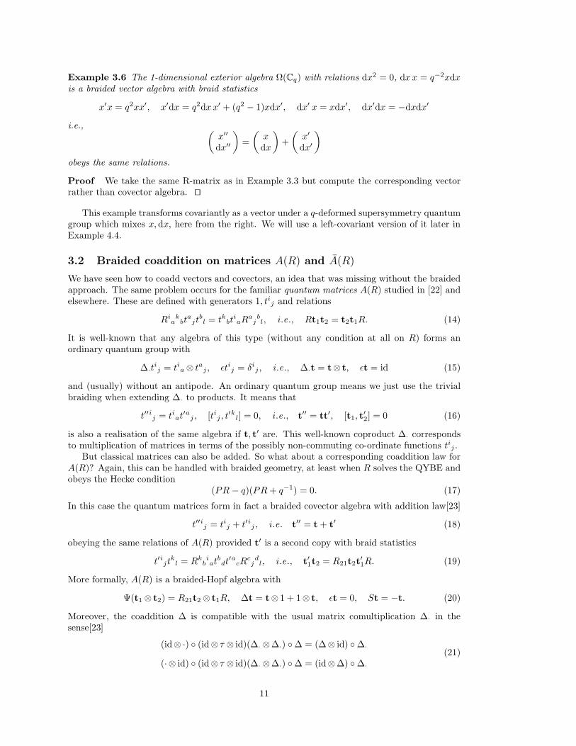
3.2 Braided coaddition on matrices A(R) and A(R)
We have seen how to coadd vectors and covectors, an idea that was missing without the braidedapproach. The same problem occurs for the familiar quantum matrices A(R) studied in [22] andelsewhere. These are defined with generators 1, tij and relations
Riakbtajtbl = tkbt
iaR
ajbl, i .e., Rt1t2 = t2t1R. (14)
It is well-known that any algebra of this type (without any condition at all on R) forms anordinary quantum group with
∆·tij = tia⊗ t
aj , ǫtij = δij , i .e., ∆·t = t⊗ t, ǫt = id (15)
and (usually) without an antipode. An ordinary quantum group means we just use the trivialbraiding when extending ∆· to products. It means that
t′′ij = tiat′aj , [tij , t
′kl] = 0, i .e., t′′ = tt′, [t1, t
′2] = 0 (16)
is also a realisation of the same algebra if t, t′ are. This well-known coproduct ∆· correspondsto multiplication of matrices in terms of the possibly non-commuting co-ordinate functions tij .
But classical matrices can also be added. So what about a corresponding coaddition law forA(R)? Again, this can be handled with braided geometry, at least when R solves the QYBE andobeys the Hecke condition
(PR − q)(PR+ q−1) = 0. (17)
In this case the quantum matrices form in fact a braided covector algebra with addition law[23]
t′′ij = tij + t′ij , i .e. t′′ = t+ t′ (18)
obeying the same relations of A(R) provided t′ is a second copy with braid statistics
t′ijtkl = Rkb
iatbdt
′acR
cjdl, i .e., t′1t2 = R21t2t
′1R. (19)
More formally, A(R) is a braided-Hopf algebra with
Ψ(t1⊗ t2) = R21t2⊗ t1R, ∆t = t⊗ 1 + 1⊗ t, ǫt = 0, St = −t. (20)
Moreover, the coaddition ∆ is compatible with the usual matrix comultiplication ∆· in thesense[23]
(id⊗ ·) (id⊗ τ ⊗ id)(∆·⊗∆·) ∆ = (∆⊗ id) ∆·
(· ⊗ id) (id⊗ τ ⊗ id)(∆·⊗∆·) ∆ = (id⊗∆) ∆·
(21)
11
where τ the usual transposition map. To see this, we have to show that t′′ in our short-handnotation obeys the same algebra relations. This is
R(t1 + t′1)(t2 + t′2) = Rt1t2 +Rt′1t′2 +RR21t2t
′1R+Rt1t
′2
(t2 + t′2)(t1 + t′1)R = t2t1R+ t′2t′1R+Rt1t
′2R21R+ t2t
′1R
which are equal because R21R = 1+(q− q−1)PR and RR21 = 1+(q− q−1)RP from the q-Heckeassumption. One can also check that Ψ extends consistently to products in such a way as to befunctorial. Details are in [23].
We have given here a direct proof of the coaddition structure on A(R). Alternatively, we canput it more explicitly in the braided covector algebra form (8)–(10) by working with the covectornotation tI = ti0 i1 for the generators where I = (i0, i1), J = (j0, j1) etc are multi-indices.Then[23]
Rt1t2 = t2t1R ⇔ tItJ = tBtAR′AIBJ ; R′I
JKL = R−1j0
i0l0k0R
i1j1k1l1
t′1t2 = R21t2t′1R ⇔ t′ItJ = tBt
′AR
AIBJ ; RI
JKL = Rl0k0
j0i0R
i1j1k1l1
(22)
puts A(R) explicitly into the form of a braided covector algebra with n2 generators. We use thebold multi-index R,R′ matrices built from our original R. They obey the conditions (3)–(6)and also the additional (113) just in virtue of the QYBE and q-Hecke condition on R. Thecorresponding braided vector algebra (11)–(13) in matrix form is
vI ≡ vi1 i0 ; R21v1v2 = v2v1R21, v′1v2 = Rv2v
′1R21. (23)
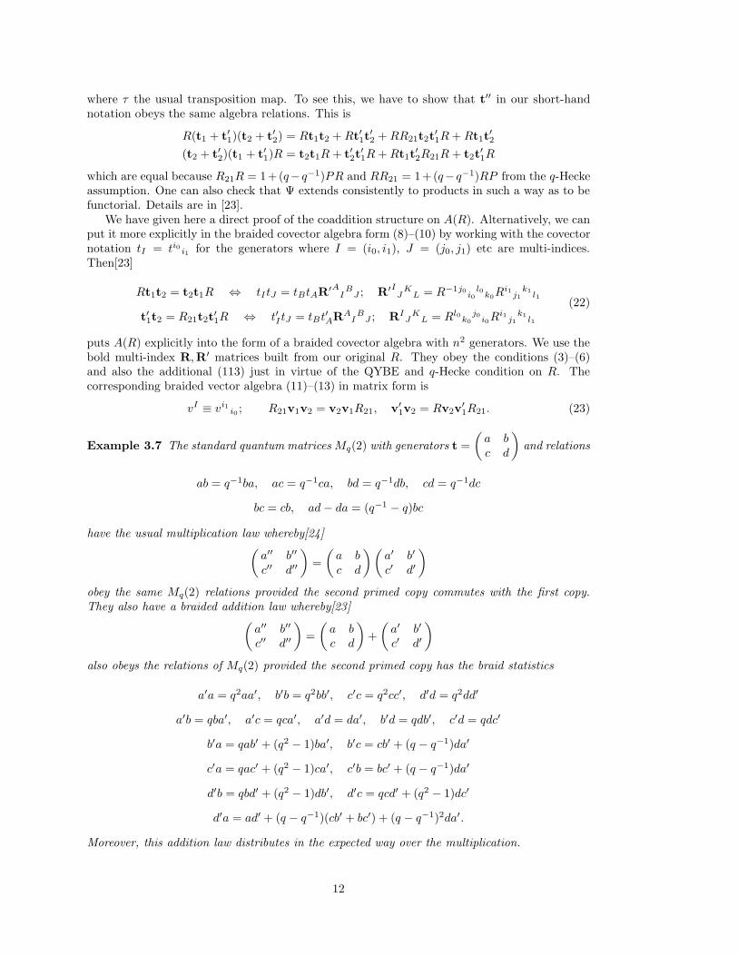
Example 3.7 The standard quantum matricesMq(2) with generators t =
(a b
c d
)and relations
ab = q−1ba, ac = q−1ca, bd = q−1db, cd = q−1dc
bc = cb, ad− da = (q−1 − q)bc
have the usual multiplication law whereby[24](a′′ b′′
c′′ d′′
)=
(a b
c d
)(a′ b′
c′ d′
)
obey the same Mq(2) relations provided the second primed copy commutes with the first copy.They also have a braided addition law whereby[23]
(a′′ b′′
c′′ d′′
)=
(a b
c d
)+
(a′ b′
c′ d′
)
also obeys the relations of Mq(2) provided the second primed copy has the braid statistics
a′a = q2aa′, b′b = q2bb′, c′c = q2cc′, d′d = q2dd′
a′b = qba′, a′c = qca′, a′d = da′, b′d = qdb′, c′d = qdc′
b′a = qab′ + (q2 − 1)ba′, b′c = cb′ + (q − q−1)da′
c′a = qac′ + (q2 − 1)ca′, c′b = bc′ + (q − q−1)da′
d′b = qbd′ + (q2 − 1)db′, d′c = qcd′ + (q2 − 1)dc′
d′a = ad′ + (q − q−1)(cb′ + bc′) + (q − q−1)2da′.
Moreover, this addition law distributes in the expected way over the multiplication.
12

Proof We take the standard R as in Example 3.1 but in the normalisation required for theq-Hecke condition (17), which is q−1 times the one shown in Example 3.1. This is not relevant tothe algebra but is needed for the correct braiding. We then compute from the formulae (14)–(20).⊔⊓
We have begun with the above quantum matrices A(R) because they are well-known quantumgroups and probably the reader has seen then somewhere before. But they are not really theexample we need for braided geometry. A more interesting algebra, which we will need inSection 7.1, is the variant A(R) studied by the author in [25]. It is defined with generators 1, xijand relations
Rkbiaxajxbl = xkbx
iaR
ajbl, i .e., R21x2x2 = x2x1R (24)
and forms a braided covector algebra if R is a Hecke solution of the QYBE, with addition lawand braid statistics[25]
x′′ = x+ x′; x′ijxkl = Ria
kbxbdx
′acR
cjdl, i .e., x′
1x2 = Rx2x′1R. (25)
More formally, it forms a braided-Hopf algebra with
Ψ(x1⊗x2) = Rx2⊗x1R, ∆x = x⊗ 1 + 1⊗x, ǫx = 0, Sx = −x (26)
To see this we check that ∆ extends to products as an algebra homomorphism to the braidedtensor product algebra, i.e. that x′′ obeys the same relations. This is checked as
R21(x1 + x′1)(x2 + x′
2) = R21x1x2 +R21x′1x
′2 +R21Rx2x
′1R+R21x1x
′2
(x2 + x′2)(x1 + x′
1)R = x2x1R+ x′2x
′1R+R21x1x
′2R21R+ x2x
′1R
which are equal by the q-Hecke assumption much as before. We also have to check that Ψ extendsconsistently to products of the generators in such a way as to be functorial. This reduces to theQYBE for R along the lines for A(R) in [23].
The usual matrix coproduct of x forms neither a quantum group nor a braided one butsomething in between. On the other hand, as before, we can put the coaddition explicitly intoour usual braided covector form by working with the multi-index notation xI = xi0 i1 . Then[25]
R21x1x2 = x2x1R ⇔ xIxJ = xBxAR′AIBJ ; R′I
JKL = R−1l0
k0j0i0R
i1j1k1l1
x′1x2 = Rx2x
′1R ⇔ x′IxJ = xBx
′AR
AIBJ ; RI
JKL = Rj0 i0
l0k0R
i1j1k1l1
(27)
puts A(R) into the form of a braided covector algebra with n2 generators. Its correspondingbraided vector algebra (11)–(13) in matrix form is A(R) again,
vI ≡ vi1 i0 ; R21v1v2 = v2v1R, v′1v2 = Rv2v
′1R. (28)
Example 3.8 [25] The q-Euclidean space algebra Mq(2) with generators x =
(a b
c d
)and
relations
ba = qab, ca = q−1ac, da = ad, db = q−1bd dc = qcd
bc = cb+ (q − q−1)ad
has a braided addition law whereby
(a′′ b′′
c′′ d′′
)=
(a b
c d
)+
(a′ b′
c′ d′
)
13

also obeys the relations of Mq(2) provided the second primed copy has the braid statistics
c′c = q2cc′, d′d = q2dd′, a′a = q2aa′, b′b = q2bb′
c′d = qdc′, c′a = qac′, c′b = bc′, d′b = qbd′, a′b = qba′
d′c = qcd′ + (q2 − 1)dc′, d′a = ad′ + (q − q−1)bc′
a′c = qca′ + (q2 − 1)ac′, a′d = da′ + (q − q−1)bc′
b′d = qdb′ + (q2 − 1)bd′, b′a = qab′ + (q2 − 1)ba′
b′c = cb′ + (q − q−1)(ad′ + da′) + (q − q−1)2bc′.
Proof We take the standard Jones invariant or SUq(2) R-matrix as in Example 3.1 but in thenormalisation required for the q-Hecke condition (17), which is q−1 times the one shown there.This is needed for the correct braiding. We then compute from the formulae (24)–(26). ⊔⊓
The interpretation of this standard example Mq(2) as q-Euclidean space will be covered inSection 7.1. The general A(R) construction is however, more general. A less standard exampleis:
Example 3.9 The algebra Mq(1|1) with generators x =
(a b
c d
)and relations
b2 = 0, c2 = 0, ba = abq, ca = q−1ac, db = −qbd, dc = −cdq−1
da = ad, bc = cb+ (q − q−1)ad
has a braided addition law whereby(a′′ b′′
c′′ d′′
)=
(a b
c d
)+
(a′ b′
c′ d′
)
also obeys the relations of Mq(1|1) provided the second primed copy has the braid statistics
a′a = q2aa′, b′b = −bb′, c′c = −cc′, d′d = dd′q−2
a′b = qba′, a′c = ca′q + (q2 − 1)ac′, a′d = da′ + (q − q−1)bc′
b′a = ab′q + (q2 − 1)ba′, b′c = cb′ + (q − q−1)2bc′ + (q − q−1)(da′ + ad′)
b′d = −q−1db′ + (q−2 − 1)bd′, c′a = qac′, c′b = bc′, c′d = −q−1dc′
d′a = ad′ + (q − q−1)bc′, d′b = −q−1bd′, d′c = −q−1cd′ + (q−2 − 1)dc′
Proof We take the Alexander-Conway R-matrix as in Example 3.2 but in the normalisationrequired for the q-Hecke condition (17), which is q−1 times the one shown. This is needed forthe correct braiding. We then compute from the formulae (24)–(26). ⊔⊓
3.3 Braided coaddition on matrices B(R)
Next we consider the braided matrices B(R) introduced and studied as a braided group by theauthor in [11][26][27]. These are defined with generators 1, uij and relations
Rkbiau
acR
cjbdudl = ukbR
bciau
adR
djcl, i .e., R21u1Ru2 = u2R21u1R. (29)
14

Such relations are perhaps more familiar as among the relations obeyed by the matrix generatorsl+Sl− of the quantum groups Uq(g) in [22] but these have many other relations too beyond (29)and are not relevant for us now. They have been used by Zumino and others to describe thedifferential calculus on quantum groups; see [26] for the full story here. We are interested insteadin (29) purely as a quadratic algebra with generators uij and these relations, which is not ingeneral a quantum group at all.
The main property of these braided matrices in [11], from which they take their name, istheir multiplicative braided group structure. We have [11]
∆·uij = uia⊗ u
aj , ǫu
ij = δij , i .e., ∆·u = u⊗u, ǫu = id
Ψ·(uij ⊗u
kl) = upq ⊗ u
mnR
iadpR
−1amqbR
ncblR
cjkd
i .e., Ψ·(R−1u1⊗Ru2) = u2R
−1⊗u1R.
(30)
It means that if u′ is another copy of B(R) then the matrix product
u′′ij = uiau′aj , i .e., u′′ = uu′ (31)
obeys the relations of B(R) also provided u′ has the multiplicative braid statistics
R−1iakbu
′acR
cjbdudl = ukbR
−1iabcu
′adR
djcl, i .e., R−1u′
1Ru2 = u2R−1u′
1R. (32)
To see this, we check
R21u1u′1Ru2u
′2 = R21u1R(R
−1u′1Ru2)u
′2 = (R21u1Ru2)R
−1R−121 (R21u
′1Ru
′2)
= u2R21(u1R−121 u
′2R21)u
′1R = u2R21R
−121 u
′2R21u1u
′1R = u2u
′2R21u1u
′1R
as required for ∆· to extend to B(R) as a braided-Hopf algebra. The other details such asfunctoriality of Ψ· can also be checked in the same explicit way[11]. This is was the first braidedgroup construction known.
Note that we have stated Ψ· implicitly. To give it explicitly (for a proper braided-group
structure) we need that R is bi-invertible in the sense that both R−1 and the second inverse Rexist. The latter is characterised by
RiablR
ajkb = δijδ
kl = Ria
blR
ajkb. (33)
If we have also that R obeys the q-Hecke condition (17) then there is also a braided-covectoralgebra structure, discovered by U. Meyer, with addition law u′′ = u+u′ and braid statistics[28]
R−1iakbu
′acR
cjbdudl = ukbR
bciau
′adR
djcl, i .e., R−1u′
1Ru2 = u2R21u′1R. (34)
More formally, B(R) is a braided-Hopf algebra with
Ψ(R−1u1⊗Ru2) = u2R21⊗u1R, ∆u = u⊗ 1 + 1⊗u, ǫu = 0, Su = −u. (35)
To see this we show as usual that ∆ extends to products as an algebra homomorphism to thebraided tensor product algebra, i.e. that u′′ obeys the same relations. This is checked as
R21(u1 + u′1)R(u2 + u′
2) = R21u1Ru2 +R21u′1Ru
′2 +R21Ru2R21u
′1R+R21u1Ru
′2
(u2 + u′2)R21(u1 + u′
1)R = u2R21u1R+ u′2R21u
′1R+R21u1Ru
′2R21R+ u2R21u
′1R
which are equal by the q-Hecke assumption (17). Functoriality of Ψ under the product mapcan also be checked explicitly by these techniques, as well as the antipode and other propertiesneeded for a braided-Hopf algebra.
15

This gives a direct proof of the (braided) comultiplication and coaddition structures on B(R).We can put the latter explicitly into the braided covector form (8)–(10) by working with themulti-index notation uI = ui0 i1 and[11][28]
R′IJKL = R−1d
k0j0aR
k1bai0R
i1cbl1R
cj1l0d
R·IJKL = Rj0a
dk0R
−1ai0k1bR
i1cbl1R
cj1l0d
RIJKL = Rj0a
dk0R
k1bai0R
i1cbl1R
cj1l0d.
(36)
Then we have
R21u1Ru2 = u2R21u1R ⇔ uIuJ = uBuAR′AIBJ
u′′ = uu′; R−1u′1Ru2 = u2R
−1u′1R ⇔ u′IuJ = uBu
′AR·
AIBJ
u′′ = u+ u′; R−1u′1Ru2 = u2R21u
′1R ⇔ u′IuJ = uBu
′AR
AIBJ .
(37)
It is easy to see that R′,R obey the conditions (3)–(6) needed for our braided covector space aswell as the supplementary ones (113) needed later for the coaddition of forms. The correspondingbraided vector algebra (11)–(13) in matrix form for the relations and additive braid statistics is
vI ≡ vi1 i0 ; v1R21v2R21 = Rv2Rv1, v′′ = v + v′; v′1R21v2R
−1 = Rv2Rv′1. (38)
A braided coaddition on the following example of a braided matrix covector space was obtainedby the author in [19] but not in such a nice R-matrix form, which is due to [28].
Example 3.10 The q-Minkowski space algebra BMq(2) with generators u =
(a b
c d
)and
relations[29][11]
ba = q2ab, ca = q−2ac, da = ad, bc = cb+ (1− q−2)a(d− a)
db = bd+ (1− q−2)ab, cd = dc+ (1− q−2)ca
has a braided multiplication law whereby[11](a′′ b′′
c′′ d′′
)=
(a b
c d
)(a′ b′
c′ d′
)
obey the same relations of BMq(2) if the primed copy does and if we use the multiplicative braidstatistics
a′a = aa′ + (1− q2)bc′, a′b = ba′, a′c = ca′ + (1− q2)(d − a)c′
a′d = da′ + (1− q−2)bc′, b′a = ab′ + (1− q2)b(d′ − a′), b′b = q2bb′
b′c = q−2cb′ + (1 + q2)(1− q−2)2bc′ − (1− q−2)(d− a)(d′ − a′)
b′d = db′ + (1 − q−2)b(d′ − a′), c′a = ac′, c′b = q−2bc′
c′c = q2cc′, c′d = dc′, d′a = ad′ + (1− q−2)bc′
d′b = bd′, d′c = cd′ + (1− q−2)(d − a)c′, d′d = dd′ − q−2(1− q−2)bc′.
Here q−1a + qd is central and bosonic[11]. At the same time we have a braided addition lawwhereby[28] (
a′′ b′′
c′′ d′′
)=
(a b
c d
)+
(a′ b′
c′ d′
)
16
obey the relations again if the primed copy does and has the additive braid statistics
a′a = q2aa′, a′b = ba′, b′b = q2bb′, c′a = ac′, c′c = q2cc′
a′c = ca′q2 + (q2 − 1)ac′, a′d = da′ + (q2 − 1)bc′ + (q − q−1)2aa′
b′a = (q2 − 1)ba′ + ab′q2, b′c = cb′ + (1− q−2)(da′ + ad′) + (q − q−1)2bc′ − (2− 3q−2 + q−4)aa′
b′d = db′ + (q2 − 1)bd′ + (q−2 − 1)ba′ + (q − q−1)2ab′, c′b = bc′ + (1− q−2)aa′
c′d = dc′q2 + (q2 − 1)ca′, d′a = ad′ + (q2 − 1)bc′ + (q − q−1)2aa′
d′b = bd′q2 + (q2 − 1)ab′, d′c = cd′ + (q2 − 1)dc′ + (q − q−1)2ca′ + (q−2 − 1)ac′
d′d = dd′q2 + (q2 − 1)cb′ + (q−2 − 1)bc′ − (1− q−2)2aa′
So we have both multiplication and addition of these braided matrices.
Proof We use the R-matrix from Example 3.1 in the q-Hecke normalisation (as in Example 3.7),which we put into (29)–(35). The normalisation and Hecke condition do not enter at all into themultiplicative braided group structure, but are needed for the additive one. ⊔⊓
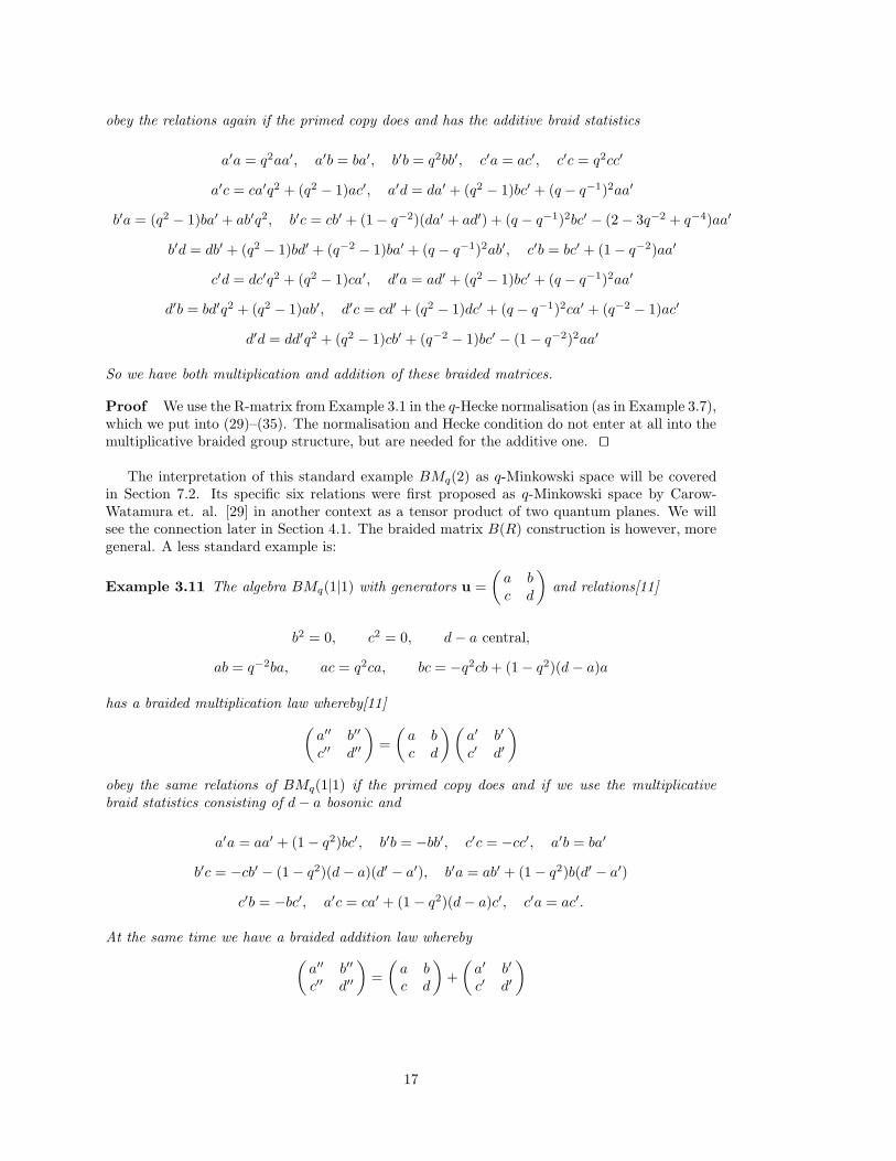
The interpretation of this standard example BMq(2) as q-Minkowski space will be coveredin Section 7.2. Its specific six relations were first proposed as q-Minkowski space by Carow-Watamura et. al. [29] in another context as a tensor product of two quantum planes. We willsee the connection later in Section 4.1. The braided matrix B(R) construction is however, moregeneral. A less standard example is:
Example 3.11 The algebra BMq(1|1) with generators u =
(a b
c d
)and relations[11]
b2 = 0, c2 = 0, d− a central,
ab = q−2ba, ac = q2ca, bc = −q2cb+ (1− q2)(d − a)a
has a braided multiplication law whereby[11]
(a′′ b′′
c′′ d′′
)=
(a b
c d
)(a′ b′
c′ d′
)
obey the same relations of BMq(1|1) if the primed copy does and if we use the multiplicativebraid statistics consisting of d− a bosonic and
a′a = aa′ + (1− q2)bc′, b′b = −bb′, c′c = −cc′, a′b = ba′
b′c = −cb′ − (1− q2)(d − a)(d′ − a′), b′a = ab′ + (1− q2)b(d′ − a′)
c′b = −bc′, a′c = ca′ + (1 − q2)(d− a)c′, c′a = ac′.
At the same time we have a braided addition law whereby
(a′′ b′′
c′′ d′′
)=
(a b
c d
)+
(a′ b′
c′ d′
)
17

obey the relations again if the primed copy does and if we use the additive braid statistics
a′a = q2aa′, a′b = ba′, a′c = q2ca′ + (q2 − 1)ac′
a′d = da′ + (q−2 − 1)bc′ + (q − q−1)2aa′, b′a = q2ab′ + (q2 − 1)ba′, b′b = −bb′
b′c = −q2cb′ ++(q − q−1)2bc′ + (1− q2)(da′ + ad′) + (2q2 − 3 + q−2)aa′
b′d = db′ + (q−2 − 1)bd′ + (q2 − 1)ba′ + (q − q−1)2ab′, c′a = ac′
c′b = −q−2bc′ + (1− q−2)aa′, c′c = −cc′, c′d = q−2dc′ + (q−2 − 1)ca′
d′a = ad′ + (q−2 − 1)bc′ + (q − q−1)2aa′, d′b = q−2bd′ + (q−2 − 1)ab′
d′c = cd′ + (q−2 − 1)dc′ + (q − q−1)2ca′ + (q2 − 1)ac′
d′d = q−2dd′ + (q−2 − 1)(cb′ + bc′) + (q − q−1)2aa′.
So we have both multiplication and addition of these non-standard braided matrices.
Proof We use the R-matrix from Example 3.2 in the q-Hecke normalisation (as in Example 3.9),which we put into (29)–(35). The normalisation and Hecke condition do not enter at all into themultiplicative braided group structure, only the additive one. ⊔⊓
This example is supercommutative in the limit q → 1 with b, c odd and a, d even. The braidstatistics also become ±1 according to the degree. Thus we recover exactly the superbialgebraM(1|1) consisting of these generators and their appropriate supercommutation relations. Thusthe notion of braided matrices really generalises both ordinary and supermatrices[11].
For completeness we note also that there is a similarity of the braided matrix algebra (29)with the ‘reflection equation’ of Cherednik [30] whose constant form is called ‘RE’ in [31]. Thispaper then went on to repeat some of the algebraic constructions in [11][26][27] in terms ofRE, with (29) as a variant RE. The braided matrix algebra B(R) is quite interesting from apurely homological point of view too, see[32]. Further results such as covariance of this braidedmatrix quadratic algebra under a background quantum group[11][27], its quantum trace centralelements[27] and a Hermitian ∗-structure[33] were likewise introduced as far as I know for thefirst time in the braided approach. We will cover the latter two properties in the next sectionand covariance in Section 6.
4 Braided linear algebra
So far we have introduced braided covectors xi, vectors vi and matrices uij , and linear structures
on the quantum matrices tij as well. Now we begin to explore the relationships between theseobjects in analogy with the usual formulae in linear algebra. This justifies our terminology furtherand shows that they all fit together into a systematic generalisation of our usual concepts.
4.1 Braided linear transformations
In braided geometry all independent objects enjoy mutual braid statistics with respect to eachother. We therefore have to extend the braiding Ψ to work between objects and not only for agiven braided group as we have done until now. This depends in fact on the applications beingmade, as we have seen already in Examples 3.10 and 3.11. For the present set of applications we
18

take[27]
Ψ(xi⊗ xj) = xn⊗ xmRminj , Ψ(vi⊗ vj) = Rim
jnv
n⊗ vm
Ψ(xi⊗ vj) = Rmi
jnv
n⊗xm, Ψ(vi⊗ xj) = xn⊗ vmR−1i
mnj
Ψ(uij ⊗xk) = xm⊗uabR
−1iamnR
bjnk, Ψ(xk ⊗u
ij) = uab⊗ xmR
nkiaR
mnbj
Ψ(uij ⊗ vk) = vm⊗uabR
ianmR
bjkn, Ψ(vk ⊗uij) = uab⊗ v
mRkniaR
−1nmbj
Ψ(uij ⊗ukl) = upq ⊗ u
mnR
iadpR
−1amqbR
ncblR
cjkd
(39)
or equivalently the braid statistics[27]
x′1x2 = x2x
′1R, v′
1v2 = Rv2v′1
x′1Rv2 = v2x
′1, v′
1x2 = x2R−1v′
1
u′1x2 = x2R
−1u′1R, x′
1Ru2R−1 = u2x
′1
R−1u′1Rv2 = v2u
′1, v′
1u2 = Ru2R−1v′
1
R−1u′1Ru2 = u2R
−1u′1R
(40)
where the primes denote the second algebra in the relevant braided tensor product algebra asin (1). The systematic way to derive these braid statistics will be covered in Section 6.1 usingthe background quantum group covariance. For the moment we verify directly that they aresuitable. They are quite natural for, but not uniquely determined by, these applications alone.
With the help of such braid statistics we show now that our braided matrices act as (braided)transformations on braided vectors and covectors, as well as on themselves. The fundamentalnotion here is that of a braided comodule algebra of B(R). On covectors for example it shouldbe an algebra homomorphism Vˇ→ Vˇ⊗B(R) to the braided tensor product algebra structureas in (1), determined now by the mutual braid statistics between braided matrices and braidedcovectors. This indeed works with the transformation
xi 7→ xa⊗uai, i .e., x′′ = xu′ (41)
obeys the same relations as the x. To see this, it is convenient to assume that PR′ is given as somefunction of PR, as for example in (7). Since nothing depends on the precise form of the function,it is clear that this is not a strong restriction. Then we compute x1u
′1x2u
′2 = x1x2R
−1u′1Ru
′2 =
x2x1R′R−1u′
1Ru′2 = x2x1R
−121 u
′2R21u
′1R
′ = x2u′2x1u
′1R
′ as required. Here we used the braidstatistics from (40) between x,u for the first and last equalities, and the relations for V (R′, R)and B(R) in the form (PR)R−1u1Ru2 = R−1u1Ru2(PR) for the middle equalities. The B(R)relations imply therefore that R′R−1u1Ru2 = R−1
21 u2R21u1R′, which could be verified directly
if PR′ is not given explicitly as a function of PR.
Example 4.1 The braided matrices BMq(2) coact from the right on the braided plane C2|0q in
the sense that
(x′′ y′′ ) = (x y )
(a′ b′
c′ d′
)
obeys the quantum plane relations if x, y do and a′, b′, c′, d′ are a copy of the braided-matrices,and provided we remember the braid-statistics
(a′ b′
c′ d′
)x =
(xa′ + (1 − q2)yc′ q−1xb′ + (q − q−1)y(a′ − d′)
qxc′ xd′ + (1− q−2)yc′
)
(a′ b′
c′ d′
)y = y
(a′ qb′
q−1c′ d′
)
19

Proof We use (41) with the standard R-matrix, computing the relevant braid statistics from(40) and deducing the coaction of BMq(2) in Example 3.10 on the usual quantum plane inExample 3.1. One can easily confirm that the transformed x′′, y′′ obey the same relations y′′x′′ =qx′′y′′. ⊔⊓
Example 4.2 The braided matrices BMq(1|1) coact from the right on the braided plane C1|1q in
the sense that
( x′′ θ′′ ) = (x θ )
(a′ b′
c′ d′
)
obeys the C1|1q relations if x, θ do and a′, b′, c′, d′ are a copy of BMq(1|1), and provided we
remember the braid-statistics(a′ b′
c′ d′
)x =
(xa′ + (1 − q2)yc′ q−1xb′ + (q − q−1)y(a′ − d′)
qxc′ xd′ + (1− q2)yc′
)
(a′ b′
c′ d′
)θ = θ
(a′ −q−1b′
−qc′ d′
)
Proof We use (41) and (40) with the non-standard R-matrix in Example 3.2, and deducingthe coaction of BMq(1|1) in Example 3.11 on it. One can easily confirm that the transformedx′′, θ′′ obey the same relations θ′′x′′ = qx′′θ′′ and θ′′2 = 0. ⊔⊓
Similarly for BMq(2) acting on the quantum superplane C0|2q in Example 3.4. It has the
same R-matrix in a different normalisation to that in Example 3.1, but this does not affect thebraid statistics which therefore comes out analogous to Example 4.1. Note that the reader hasseen quantum matrices characterised as transformations of the two types of quantum plane inManin’s lectures[24]. In our case we have non-trivial braid statistics and because of this weobtain the braided matrices BMq(2) instead. This is the general principle behind the processof transmutation as explained in the Appendix. Note also that it is only in the Hecke case that
two quantum planes such as C2|0q and C
0|2q are enough for this. More generally one needs to
consider all quantum planes for each choice of eigenvalue of PR in (7). Braided covectors aloneare enough to do the job of characterising the braided matrices as (braided) transformations inthis way provided we consider the various possibilities for them.
In the same way, we have braided coactions of B on the braided vectors vi and on the braidedmatrices uij itself. Here B is a braided group with antipode which we must make from B(R)in a way compatible with the braidings. This is possible for regular R in the sense explainedin Section 6.1. The braided antipode S can be found either by hand or by the systematictransmutation technique in the Appendix. Assuming it, the relevant transformations are[27]
vi 7→ (1⊗Suia)(va⊗ 1), uij 7→ (1⊗Suia)(u
ab⊗u
bj) i .e., v→ u′−1v, u→ u′−1uu′ (42)
where the expressions are written in the braided tensor product algebra V⊗B or B(R)⊗Brespectively. In the compact notation u′ denotes the generator of the B factor. The secondof the transformations here is the braided adjoint action and can be used as a foundation for atheory of braided-Lie algebras[9].
Next we show that the tensor product of a quantum covector with a quantum vector,when treated with the correct braid statistics, is a braided matrix, i.e. the map B(R) →V (R′, R)⊗V (R′, R) given by[27]
uij 7→ vi⊗ xj , i .e., u 7→ vx′ =
v1x′1 · · · v1x′n...
...vnx′1 · · · vnx′n
(43)
20

is an algebra homomorphism provided we use the braid statistics from (40). Again, this resultfrom [27] is most easily checked under the mild assumption that PR used for the braided covec-tors and vectors in Section 3 is given as some function of PR′. Then we have R21v1x
′1Rv2x
′2 =
R21v1v2x′1x
′2 = f(PR′)Pv1v2x
′1x
′2 = v2v1f(1)x
′1x
′2 = v2v1x
′1x
′2f(PR
′) = v2v1x′2x
′1R =
v2x′2R21v1x
′1R. The first and last equalities use the braid statistics relations. The middle
equalities use the defining relations in the algebras V (R′, R), V (R′, R). Hence vx′ is a realisa-tion of the braided matrices B(R). If PR is not given explicitly as some function of PR′ thenthe proposition typically still holds but has to be verified directly according to the form in whichPR′, PR are given. An example is[27]
BMq(2)→ C2|0
q−1⊗C2|0q (44)
which relates the braided-matrix point of view which we will later adopt as a definition of q-Minkowski space (see Example 3.10) with an independent approach pioneered in [34][29][35].
It is also easy to see that the ‘inner product’ element
x′ivi = vbx′aϑ
ab = Trvx′ϑ; ϑij = Ria
aj (45)
in the braided tensor product algebra V (R′, R)⊗V (R′, R) is central and bosonic with respectto the multiplicative braid statistics[27]. This applies also to c1 = Truϑ as one would expect inview of (43). The trace elements in Examples 3.10 and 3.11 are of just this form. More generallyone has that all the powers ck = Trukϑ are bosonic and central in B(R)[27]. This means ofcourse that
ckuij = uijck, u′ijck = cku
′ij , c′ku
ij = uijc
′k (46)
in the algebras B(R) and B(R)⊗B(R) respectively. The first equation is similar to the construc-tion of Casimirs of Uq(g) in [22] in another context, while the latter two equations about thebosonic nature are new features of the braided theory in [27].
One can show (again as an application of transmutation) that the bosonic central elements inthe braided matrices B(R) generate a subalgebra (are closed under addition and multiplication).In this subalgebra one can expect to find interesting bosonic central elements such as the braided-determinant det(u). This should be group-like in the sense
∆det(u) = det(u)⊗ det(u), ǫdet(u) = 1 (47)
with respect to the braided comultiplication. For example, in the 2-dimensional case it means
det
((a b
c d
)(a′ b′
c′ d′
))= det
(a b
c d
)det
(a′ b′
c′ d′
)(48)
where we use the multiplicative braid statistics as in (40). One can also expect
det(vx′) = 0 (49)
from our above picture of vx′ as a rank-1 braided matrix. There is also a general formula fordet using the R-matrix formula for the epsilon tensor in Section 5.7. All of this suggests afairly complete picture of our braided vectors, covectors and matrices in terms of braided linearalgebra[27].
4.2 Gluing or direct sum of braided vectors
Next we consider some finer points of linear algebra in our braided framework. The first concernshow to tensor product braided groups. The braided tensor product algebra and braided tensorproduct coalgebra (defined in an obvious way again using the braiding) do not in general fittogether to form a braided group: one must also ‘glue together’ the braidings of the two braidedgroups.
21

Such a gluing construction has been found by the author and M. Markl in [36] for the Heckecase. Firstly, if R,S are two solutions of the QYBE obeying the Hecke condition (17) then sois[36]
R⊕q S =
R 0 00 1 (q − q−1)P 00 0 1 00 0 0 S
. (50)
Here P is the permutation matric. The dimensions of R,S need not be the same. Such aphenomenon is encountered from time to time in the R-matrix literature, see [37] where Hecke R-matrices were extensively studied, although not as far as I know as a systematic gluing operation.
Many consequences of this associative gluing operation ⊕q are then explored in [36]. Amongthem, it is shown that
V λ(R ⊕q S) = V λ(R)⊗λV λ(S); λ = q or − q−1. (51)
Recall that in the Hecke case there are two natural choices for our braided covector data, whichwe label by λ: we keep R,S fixed in the Hecke normalisation and take (Rλ, λ−1R) for (R,R′) inSection 3.1. Likewise (Sλ, λ−1S) for V λ(S). The ⊗λ is the braided tensor product with respectto a braiding given by the power of the braided covector generators (the scaling dimension) muchas in the braided-line example in Section 2. Explicitly, the isomorphism (51) is given by writingthe generators of V λ(R ⊕q S) as (xi, yI) say for appropriate ranges of indices according to thedimensions of R,S. Then its relations are
λx1x2 = x2x1R, λy1y2 = y2y1S, yIxj = λxjyI , i .e., y1x2 = λx2y1 (52)
which is the right hand side of (51).Note that our algebras are like those generated by the co-ordinate functions on row vectors.
Their tensor product is therefore like the direct sum of the underlying braided vector spaces. Forexample,
Cn|0q ⊗qC
m|0q = C
n+m|0q , C
0|nq ⊗(−q−1)C
0|mq = C
0|n+mq
as is clear from the well-known form of these spaces. The above gluing however, works quitegenerally for arbitrary R,S of Hecke type.
This gluing is an example of a more general construction of rectangular quantum matricesA(R : S) introduced in [36]. These are defined with generators 1, xiI say and relations
RiakbxaJx
bL = xkBx
iAS
AJBL, i .e., Rx1x2 = x2x1S. (53)
and a braided addition law x′′ = x+ x′ with braid statistics[36][23]
x′iJxkL = Rkb
iaxbDx
′aCS
CJDL, i .e., x′
1x2 = R21x2x′1S. (54)
They are not in general quantum groups but instead we have partial comultiplication maps
∆R,S,T : A(R : T )→ A(R : S)⊗A(S : T ), ∆xiα = xiI ⊗ xIα, i .e., ∆x = x⊗x (55)
for any three Hecke solutions R,S, T of the QYBE, corresponding to matrix multiplication ofrectangular matrices. We associate the R-matrices R,S to the rows and columns of A(R : S) andthere is a comultiplication when the rows match the columns to be contracted with. There is alsodistributivity generalising (21) and expressing linearity of ∆R,S,T with respect to the coaddition.Finally, we can regard the rectangular quantum matrices A(R : S) as a braided covector space asin Section 3.1 with multi-index R′,R now built from R,S, see [23]. The corresponding braidedvector space is A(S21 : R21).
It is clear that setting R = (q) or (−q−1) (the 1-dimensional Hecke R-matrices) recovers thebraided covectors as 1 × n rectangular quantum matrices V λ(R) = A(λ : R). The other case
22

A(R : λ) of n× 1 rectangular quantum matrices recovers a left handed version Rv1v2 = v2v1λ
of the braided vectors. We have given conventions in Section 3.1 in which everything is right-covariant under a background quantum group, while these left-handed vectors are left-covariantby contrast. The general A(R : S) is bicovariant using the maps (55) for comultiplicationfrom the left or right by A(R : R) = A(R) and A(S : S) = A(S). The diagonal case ofthe rectangular quantum matrices are of course the usual quantum matrices of [22]. Anotherexample is A(R21 : R) = A(R) which is the variant from [25]. Finally, we have good behaviourof this construction under gluing as[36]
A(R : S ⊕q T ) = A(R : S)R⊗A(R : T ), ykαxiJ = Ria
kbxaJy
bα, i .e., y2x1 = Rx1y2 (56)
A(R⊕q S : T ) = A(R : T )⊗TA(S : T ), wJ δv
iγ = viαw
JβT
βδαγ , i .e., w1v2 = v2w1T (57)
which generalises the above. Here x ∈ A(R : S), y ∈ A(R : T ) which we view as (x y) and
v ∈ A(R : T ), w ∈ A(S : T ) which we view as
(v
w
). The braided tensor products are defined
with braidings given by R, T respectively, which we have shown as the braid statistics betweenthe two factors in each case.
Example 4.3 We can horizontally glue two quantum plane column vectors to give a quantummatrix, or vertically glue two quantum plane row vectors to achieve the same:
Mq(2) = C2|0q Rgl2
⊗C2|0q 〈
(a b
c d
)〉 = 〈
(a
c
)〉⊗〈
(b
d
)〉
= C2|0q ⊗Rgl2
C2|0q
i .e.,= 〈( a b )〉⊗〈( c d )〉
where Rgl2 = (q)⊕q (q) is the standard R-matrix as in Example 3.1 but in the Hecke normalisa-tion. This is one way to derive its relations as quoted in Example 3.7.
Proof For the first case we use (56) with R the standard R-matrix as in Example 3.1 and 3.7.
Then A(R : q) = C2|0q as a left-covariant column vector and A(R : q)R⊗A(R : q) = A(R :
(q) ⊕q (q)). But R = (q) ⊕q (q) so the latter is just A(R) = Mq(2). Likewise for the second
example we have A(q : R) = C2|0q as a right-covariant row vector and A(q : R)⊗
RA(q : R) =
A((q) ⊕q (q) : R) = A(R) = Mq(2) by (57). The explicit identification of the generators for thetwo cases is shown on the right, where 〈 〉 denotes the algebra generated. ⊔⊓
We could equally well glue n rows of the quantum planes Cn|0q or n columns to arrive at the
n × n quantum matrices Mq(n). If we glue m rows or columns then we arrive at rectangularquantum matrices A(Rglm : Rgln) or A(Rgln : Rglm) etc. Such decomposition properties of thestandard quantum matrices Mq(n) or SLq(n) are to some extent known in other contexts, butrecovered here systematically as part of a general framework. For a less standard example we
could just as easily glue a row vector quantum plane C2|0q and a ‘fermionic’ row vector C
0|2q say,
i.e. glue Examples 3.1 and 3.4 vertically. Or we could glue horizontally two copies of the mixed
quantum plane C1|1q in Example 3.2. Either way, the result by the gluing theorems (56)–(57)
will be the ‘rectangular’ quantum matrices A(Rgl1|1 : Rgl2) where Rgl1|1 = (q) ⊕q (−q−1) is the
Alexander-Conway R-matrix as in Example 3.2, in the Hecke normalisation. Clearly we havesome powerful gluing technology which we can use any number of ways. We content ourselveshere with a concrete application of such ideas to quantum differential geometry.
Example 4.4 We can horizontally glue two copies of the (left-handed version of) the 1-dimensionalquantum exterior algebra in Example 3.6 to obtain the left-handed quantum exterior algebra onthe quantum plane as a rectangular quantum matrix
Ω(C2|0q ) = Ω(Cq)RΩ⊗Ω(Cq), i .e., 〈
(x y
dx dy
)〉 = 〈
(x
dx
)〉⊗〈
(y
dy
)〉
23

where RΩ is the R-matrix as in Examples 3.3 and 3.6, in the Hecke normalisation. The rectan-
gular quantum matrix Ω(C2|0q ) = A(RΩ : Rgl2) transforms covariantly under a quantum group
MΩq (1|1) = A(RΩ) for each column and under Mq(2) for each row. It has relations
yx = qxy, (dx)2 = 0, (dy)2 = 0, dydx = −q−1dxdy
dxx = q2xdx, dx y = qydx, dy y = q2ydy, dy x = (q2 − 1)dx y + qxdy
from (53) and a braided addition law from (54) whereby
(x′′ y′′
dx′′ dy′′
)=
(x y
dx dy
)+
(x′ y′
dx′ dy′
)
obeys the same relations of Ω(C2|0q ) provided the primed copy has the braid statistics
x′x = q2xx′, x′y = qyx′, y′x = (q2 − 1)yx′ + qxy′, y′y = q2yy′
x′dx = dxx′, x′dy = q−1dy x′, y′dx = (1− q−2)dy x′ + q−1dx y′, y′dy = dy y
dx′ x = (q2 − 1)dxx′ + q2xdx′, dx′ y = (q − q−1)dy x′ + qydx′
dy′ x = (q − q−1)2dy x′ + (q − q−1)(dx y′ + qydx′) + qxdy′, dy′ y = (q2 − 1)dy y′ + q2ydy′
dx′dx = −dxdx′, dx′dy = −q−1dydx′
dy′dx = (q−2 − 1)dydx′ − q−1dxdy′, dy′dy = −dydy′
Proof We take Ω(Cq) = A(RΩ : q) which is a left-covariant vector version of Example 3.6 (ithas the opposite algebra). Then Ω(Cq)RΩ⊗Ω(Cq) = A(RΩ : q)RΩ⊗A(RΩ : q) = A(RΩ : Rgl2)as an example of (56). We compute its relations from (53) and obtain the algebra generatedby x, y, dx, dy previously proposed as a natural covariant differential calculus for the quantumplane in [38][39] and for which a coaddition was recently proposed in [40]. By obtaining it asa rectangular quantum matrix, we know from the general theory above (without any work) notonly that it is covariant under the usual Mq(2) in Example 3.7 whereby
(x y
dx dy
)(a b
c d
);
(a b
c d
)bosonic
obeys the Ω(C2|0q ) relations, which is the usual picture (cf. Manin’s lectures), but also that it is
covariant under a different quantum group MΩq (1|1) with relations
ba = ab, ca = acq2, db = −bd, dc = −q−2cd
cb = bcq2, ad− da = bc(1− q2), b2 = 0, c2 = 0
whereby (a b
c d
)(x y
dx dy
);
(a b
c d
)bosonic
obeys the same relations of Ω(C2|0q ) as well. The quantum matrix A(RΩ : Rgl2) is ‘rectangular’
in that its rows and columns transform under different quantum groups (i.e., have a differentflavour) even though they have the same dimension. Moreover, we also know from [36] that everyrectangular quantum matrix in our setting has a braided addition law. We compute the requiredbraid-statistics at once from (54). They are the same as Examples 3.1 and 3.4 for the two rows
24

and (the opposite version of) Example 3.6 for each column, but include cross statistics such asdy′ x also. ⊔⊓
The same remarks apply in n-dimensions by iterated gluing, or indeed for the quantum planeassociated to any Hecke R-matrix. We have taken so far the view of horizontal gluing (of theexterior algebras for each dimension). We can also take the vertical gluing point of view wherebywe glue the position co-ordinates and the basic forms as
Ωq(R) = V q(R)⊗qRVˇ−q−1(R) = A(RΩ : R), i .e., 〈
(x1 · · ·xn
dx1 · · · dxn
)〉 = 〈xi〉⊗qR〈dxi〉
qx1x2 = x2x1R, dx1dx2 = −qdx2dx1R, dx1 x2 = qx2dx1R
(58)which works for general Hecke R. Note that in [36] we also gave generalisations of the gluingprocedure (50). One of these generalisations allows operators in the inner diagonal of (50)and it is this slightly generalised version which we use to obtain RΩ = (q) ⊕q (−q
−1). Thecorresponding version of (57) involves qR in the braided tensor product. This extra factor of qis needed to ensure that our notation is consistent with d2 = 0 and a usual graded Leibniz rule.We arrive at a version of the quantum exterior algebra Ωq(R) as in [39] but obtained now as arectangular quantum matrix. As such, its A(R) covariance from the right is automatic, while atthe same time we see automatically covariance from the left underMΩ
q (1|1). The quantum group
MΩq (1|1) clearly has some super-like qualities and, indeed, there is a theory of superisation which
converts it strictly into a super-quantum group along the lines developed by the author and M.J.Rodriguez-Plaza in [41]. It is then a q-deformation of a hidden supersymmetry in the exterioralgebra of Rn. Also automatic is that Ωq(R) has a braided addition law from (54). We return tosuch exterior algebras from a more general and more constructive point of view in Section 5.7.The recent papers [40][42] on exterior algebras in the braided setting likewise go beyond the Heckecase covered by the gluing theory in[36]. In a somewhat different direction but also related togluing, see [43]. One can envision many other applications also of the gluing theory, such asformulating quantum path spaces and function spaces as infinitely iterated gluings, see [23].
Finally, we can consider the quantum groups A(R⊕q S). From the above they comes out asgenerated by four block matrices and block relations[36]
t =
(a b
c d
), a ∈ A(R), b ∈ A(R : S), c ∈ A(S : R), d ∈ A(S)
Ra1b2 = b2a1, c1a2 = a2c1R, Sc1d2 = d2c1, d1b2 = b2d1S
b1c2 = c2c1, a1d2 − d2a1 = (q−1 − q)Pc1b2.
(59)
This is a ‘blocked form’ of the quantum matrices Mq(2) in Example 3.7, where the generatorsare themselves now rectangular quantum matrices as shown.
We see then that these general braided tensor product constructions provide analogues of theusual constructions whereby matrices can be multiplied and blocked into smaller ones. There isa further theory for gluing or decomposition of braided matrices which remains to be studied,connecting with the results (43)–(44) in Section 4.1. Also, it would be nice to go beyond theHecke case as well as to use other possible ‘templates’ in (50) such as the 8-vertex R-matrix inplace of the standard 6-vertex one used in [36].
4.3 Braided metric
Next we consider the situation that our braided vector and covector algebras are isomorphic.Recall that this is the true meaning of the metric in differential geometry. So to complete ourpicture we follow [28] and define a braided metric as a matrix ηij such that
xi = ηiava, vi = xaη
ai (60)
25

is an isomorphism of braided-Hopf algebras. Here ηij is the inverse transpose characterised byηjaη
ia = δij = ηajηai.
There are two aspects to this definition, one for the algebra isomorphism and one for anequivalence of the braiding so that the braided tensor product algebras are also isomorphic.These immediately come out respectively as[28]
ηiaηjbR′akbl = R′a
ibjηakηbl, ηiaηjbR
akbl = Rai
bjηakηbl (61)
We will see later in Section 6.1 that the above constructions are generally covariant under abackground quantum group. It is natural to demand that η preserves this (is an intertwiner forthe coaction). This implies the second of (61) and other relations too between η and R whichwe could take along with (61) as axioms for a covariant metric. These include[44]
ηkaRijal = λ−2R−1i
jakηal, ηkaR
ijal = λ2Rij
akηal (62)
Rajklηai = λ−2ηjaR
−1aikl, Raj
klηai = λ2ηjaR
aikl (63)
obtained by the methods in Section 6.1. The parameter λ which shows up here is called thequantum group normalisation constant[27] and depends on the R-matrix. Finally, we can alsorequire our metric to be symmetric in some sense. The natural condition is to use the samenotion as the sense in which the braided covector and vector algebras are commutative, i.e.,
ηbaR′aibj = ηij . (64)
The corresponding equations in terms of the inverse transposed metric ηij are
ηiaηjbR′kalb = R′i
ajbηakηbl, ηiaηjbRka
lb = R′i
ajbηakηbl (65)
ηlaRijka = λ−2R−1i
jlaηal, ηlaRij
ka = λ2Rij
laηak (66)
Riaklηaj = λ−2ηiaR−1j
akl, Ria
klηaj = λ2ηiaRja
kl (67)
R′iajbηba = ηij . (68)
We will see in Section 5.6 how to construct quantum metrics as an application of braided-differentiation. It can also be obtained from knowledge of the ∗-structure. We describe thisnext.
4.4 Braided ∗-structures
If we think of our algebras above as like the co-ordinate functions on a manifold or (equallywell) as like a quantum system, we need to specify an operation ∗ from the algebra to itselfwhich is like pointwise complex conjugation. It should be antilinear, square to 1 and be anantialgebra homomorphism, i.e., should make our algebras into ∗-algebras. Such a structure isimportant in the non-commutative or quantum case because it determines what it means for arepresentation of our algebras to be ‘real’. Namely in the quantum case ∗ should map over toHermitian conjugation, which requirement generalises the notion of a unitary representation of agroup. Since we do not have either points or groups, we should specify ∗ axiomatically by theseand further properties.
For a braided group the most useful further axioms (as determined by experience rather thanby abstract considerations) appear to be [33]
(∗⊗∗) ∆ = τ ∆ ∗, ǫ ∗ =¯ ǫ, ∗ S = S ∗ (69)
where τ denotes the usual transposition.Whether or not our braided vectors, covectors and matrices etc have a natural ∗-structure
depends on the particular algebras. These in turn depend on the chosen R,R′ matrices. We
26
discuss here what can be said at this general level depending on the general properties of thesematrices: there may be other possibilities too for individual algebras when one looks at them byhand. There are two useful cases[33]
Rijkl = Rlkji (real type I), Rijkl = R−1j
ilk (antireal type I). (70)
There are also type II cases needed to cover q-Minkowski space if we treat it as a braided covectoralgebra[45]. We use the same classification for R′.
It is natural to ask our metric, when it exists, to respect ∗. We require
ηij = ηji (71)
which is compatible with the various relations (65)–(68) when λ is real, for either the real orantireal type I case for R,R′. Then one can check that
x∗i = xaηai (72)
makes V (R′, R) into a ∗-braided group obeying the above axioms[45]. The braided vector algebrais isomorphic when there is a metric, so it has a corresponding operation vi∗ = ηiav
a by thisisomorphism. There is also a second ∗-structure given on the vi (say) by vi∗ = ηaiv
a which isneeded for the duality theory in[45].
When there is no metric, it is more reasonable to think of our braided covectors and vectorsas holomorphic and antiholomorphic. This is because rather than a ∗-structure as above, thereis a natural map from one to the other as x∗i = vi. The details and some non-trivial theorems inthis direction are in [45]. This holomorphic situation is the one that applies to the most simple
examples such as the quantum plane C2|0q .
Next, we look at ∗-structures for our other objects. We concentrate on R of real type I, whichholds for our standard Rgl2 and similar R-matrices when q is real. In the case of the quantummatrices A(R) it is known that these often have a ‘unitary’ ∗-structure[46]
tij∗ = Stji (73)
at least when made into Hopf algebras with antipode S for the multiplicative coproduct. Usuallythe same formula can be used at the bialgebra level too. For example, the usual quantum matricesMq(2) in Example 3.7 have a standard ∗-structure
(a∗ b∗
c∗ d∗
)=
(d −q−1c
−qb a
)(74)
when q is real. This is the ∗-structure familiar for SUq(2) except that the same formula workseven when we do not demand the q-determinant relation. Of course, we do not obey the antipodepart of Woronowicz’ axioms for a Hopf ∗-algebra[46], but only the properties for a ∗-bialgebrawith respect to comultiplication.
At least in the Hecke case we also have the possibility of a second approach to the ∗-structureon A(R), namely to write it as a braided covector space as in Section 3.2. Then the biggermulti-index matrices R,R′ in (22) will also be real type I, and hence when there is a quantummetric ηIJ we will have a ∗-structure by the above. This second approach ensures that we obeythe axioms (69) for the additive braided group structure.
Example 4.5 The usual quantum matrices Mq(2) in Example 3.7 have a braided covector ∗-structure (
a∗ b∗
c∗ d∗
)=
(−qd c
b −q−1a
)
when q is real.
27
Proof We regardMq(2) as a 4-dimensional braided covector space and use the quantum metric
ηIJ =
0 0 0 −q−1
0 0 1 00 1 0 0−q 0 0 0
.
One can check that it obeys the conditions in Section 4.3 with respect to R,R′ and λ = q−1, aswell as the condition (71). Then we get the braided covector ∗-structure from (72). ⊔⊓
The braided covector approach works just as well on the variants A(R). The multi-indexmatrices R,R′ from (27) are again of real type I and a quantum metric obeying (71) then givesus a braided covector ∗-structure. This includes our standard example of q-Euclidean spaceMq(2) from Example 3.8. We describe it further in Section 7.1. Also, there is a systematicprocess of twisting which turns A(R) into A(R). It turns the multiplicative ∗-structure on thematrix generators t of the former into the braided covector ∗-structure on the generators x ofthe latter. By this general theory one could begin with the usual (74) on Mq(2), take the sameform for the ∗-structure on Mq(2) and hence by (72) deduce its quantum metric ηIJ . This is theline taken by the author in [25].
For ∗ structures on braided matrices B(R) the discussion is simpler because we do not needto consider an antipode. This topic was covered in [33] where it was shown that for R of realtype I, we have a braided ∗-bialgebra of Hermitian type
uij∗ = uji (75)
with respect to the braided comultiplication in the axioms (69). Firstly, it is easy to see thatB(R) for real-type R is a ∗-algebra. See [33] or other places where the algebra relations havebeen studied. Next note that B(R)⊗B(R) has a natural ∗-structure defined not in the obviousway but by[33]
(b⊗ c)∗ = c∗⊗ b∗, ∀b, c ∈ B(R), i .e. uij∗ = u′ji, u′ij
∗ = uji
on the generators. We just have to check that this is compatible with the relations of the braidedtensor product. Thus
(R−1iakbu
′acR
cjbdudl)∗ = u′ldR
dbjcucaR
−1bkai
= RlajbubcR
−1adciu
′dk = (ukdR
−1icdau
′cbR
bjal)∗
as required. We used the multiplicative braid statistics in Section 3.3. After this we just haveto note that the multiplicative ∆· is a ∗-algebra map on the generators and hence extends toproducts as a ∗-algebra map.
As before, a second way is to think of our braided matrices as a braided covector space, asexplained in Section 3.3. We have R,R′ from (36) obeying some different properties, called typeII in [45] but again leading to a ∗-braided group structure on our covectors, this time with (75).For a direct check, the computation is like the above but this time with Meyer’s additive braidstatistics:
(R−1iakbu
′acR
cjbdudl)∗ = u′ldR
dbjcucaR
−1bkai
= RlajbubcR
ciadu
′dk = (ukdR
daicu
′cbR
bjal)∗
The braided coaddition extends to products as a ∗-algebra homomorphism to this braided tensorproduct algebra. It is remarkable that the same Hermitian form (75) works for both comultipli-cation and coaddition, making B(R) a ∗-braided group in two ways.
Note that under coaddition, the transposition τ in (69) might be unexpected – it is notvisible classically because the coaddition is then cocommutative (symmetric in its output). But
28

the comultiplication on the other hand is not symmetric and here a τ really is to be expected forHermitian matrices: classically the product of two Hermitian matrices M,N is not Hermitianbut rather obeys (MN)∗ = NM .
In addition, there is a strict relation of transmutation in [33] which obtains this Hermitian∗-structure on B(R) from the multiplicative unitary-like one on A(R). There is also a theoryof twisting in [25] which turns the braided covector ∗-structure of A(R) into B(R). So all threealgebras are connected by general theory. The Hermitian form obviously means that the standard2 × 2 braided matrices BMq(2) in Example 3.10 should be regarded as a natural q-Minkowskispace. We can deduce its quantum metric ηIJ from this ∗-structure and (72). It is covered inSection 7.2. The twisting relation between Mq(2) and BMq(2) becomes ‘quantum Wick rotation’in this context[25].
Once one has a suitable ∗-structure on a braided space, it is natural to ask about its impli-cations for the various other constructions in braided geometry, such as those to be describedbelow. This is covered in [45], to which we refer the interested reader. Not all problems in thisdirection are yet solved.
5 Braided analysis
So far we have described how to q-deform Rn as a braided covector or vector space and developed
the associated concepts of linear algebra. We now proceed to the first steps of ‘braided analysis’ onsuch spaces. We concentrate first on understanding braided differentiation from [20]. This thendetermines braided exponentials, braided-Gaussians, braided-integration and braided-differentialforms etc., i.e. some of the remaining basic concepts for ‘analysis’ on Rn.
5.1 Braided differentiation
The next stage after braided addition and linear algebra is to make an infinitesimal addition,which leads to the concept of differentiation. We can think of the coaddition (9)–(10) on ourcovectors xi equally well as a braided coaction of one copy of the covectors on another, i.e. asa global translation. If we denote the generators of the coacting copy by a then the content ofSection 3.1 is that a + x also obeys the relations of a braided covector provided we rememberthe braid statistics x1a2 = a2x1R. We are now ready to follow the ideas of I. Newton and definedifferentiation ∂i : V (R′, R)→ V (R′, R) as an infinitesimal translation[20]
∂if(x) =(a−1i (f(a+ x)− f(x))
)a=0≡ coeff of ai in f(a+ x). (76)
We take the linear part in ai, which is some function of x and does not depend in fact on invertingai or taking a limit. For example, on monomials we have
coeffai ((a1 + x1)(a2 + x2) · · · (am + xm))
= coeffai (a1x2 · · ·xm + x1a2x3 · · ·xm + · · ·+ x1 · · ·xm−1am)
= coeffai(a1x2 · · ·xm(1 + (PR)12 + (PR)12(PR)23 + · · ·+ (PR)12 · · · (PR)m−1,m))
giving us the result[20]
∂i(x1 · · ·xm) = ei1x2 · · ·xm [m;R]1···m , ∂ixi1 · · ·xim = δij1xj2 · · ·xjm [m;R]j1···jmi1···im
(77)
where ei is a basis covector (ei)j = δij and[20]
[m;R] = 1 + (PR)12 + (PR)12(PR)23 + · · ·+ (PR)12 · · · (PR)m−1,m (78)
is a certain braided integer matrix living in the m-fold matrix tensor product of Mn.
29
The operators ∂i have upper indices so one should hope that they obey the relations of thebraided vectors vi in Section 3.1. This is indeed true and means that it defines an action ofV (R′, R) on V (R′, R) given by this differentiation. We have[20]
∂i∂kx1 · · ·xm = ek1ei2x3 · · ·xm [m− 1;R]2···m [m;R]1···m
R′iakb∂b∂ax1 · · ·xm = R′i
akb∂bea1x2 · · ·xm [m;R]1···m
= R′iakbea1eb2x3 · · ·xm [m− 1;R]2···m [m;R]1···m
= ek1ei2x3 · · ·xm(PR′)12 [m− 1;R]2···m [m;R]1···m
which are equal due to the identity
[m− 1;R]2···m [m;R]1···m = (PR′)12 [m− 1;R]2···m [m;R]1···m (79)
proven in [20], to which we refer for further details.Moreover, the braided covectors are braided-covariant under this action. The concept is much
like the covariance in Section 4.1: we use braid statistics. In fact we need the inverse braidingΨ−1 as given between vectors and covectors in (39)–(40). As usual, it extends to products insuch a way as to be compatible with the product map. This consideration translates into thebraided-Leibniz rule[20]
∂i(ab) = (∂ia)b+ ·Ψ−1(∂i⊗ a)b
Ψ−1(∂i⊗x1 · · ·xr) = ei1x2 · · ·xrxr+1(PR)12 · · · (PR)r,r+1⊗ ∂r+1.
(80)
There is an abstract or diagrammatic derivation for this based on duality[3]. For a direct proofone has[20]
(∂ix1 · · ·xr)xr+1 · · ·xm +Ψ−1(∂i⊗x1 · · ·xr)xr+1 · · ·xm
= ei1x2 · · ·xr [r;R]1···r xr+1 · · ·xm
+ei1x2 · · ·xrxr′+1(PR)12 · · · (PR)r,r′+1∂r′+1xr+1 · · ·xm
= ei1x2 · · ·xrxr+1 · · ·xm [r;R]1···r+ei1x2 · · ·xrxr+1(PR)12 · · · (PR)r,r+1xr+2 · · ·xm [m− r;R]r+1···m
where we use (77) to evaluate the differentials. The primed r′ + 1 labels a distinct matrix spacefrom the existing r+1 index. These are then identified by the er+1 brought down by the actionof ∂r′+1. The resulting expression coincides with ei1x2 · · ·xrxr+1 · · ·xm [m;R]1···m due to thebraided-integer identity[20]
[r;R]1···r + (PR)12 · · · (PR)r,r+1 [m− r;R]r+1···m = [m;R]1···m . (81)
Another way to express this braided-Leibniz rule is in terms of commutation relations betweendifferentiation and position operators xi : V (R′, R) → V (R′, R) acting by multiplication fromthe left by xi. The braided-Leibniz rule applied to ∂i(xjf(x)) gives at once that
∂ixj − xaRajib∂b = δij , i .e. ∂1x2 − x2R21∂1 = id (82)
as operators on V (R′, R). This is obviously the point of view that could be called ‘braidedquantum mechanics’. Indeed, we showed in [20] that there is an abstract braided Weyl algebradefined by
x1x2 = x2x1R′, p1p2 = R′p2p1, p1x2 − x2R21p1 = id (83)
with (82) as an operator realisation. The construction was as a braided cross product[47] andgeneralised the standard GLq(n) case that had been considered before[38][48].
30
Example 5.1 The braided-line Cq at the end of Section 2 has braided differentiation
∂xm = xm−1(1 + q + · · ·+ qm−1) = [m; q]xm−1 ⇒ ∂f(x) =f(qx)− f(x)
(q − 1)x.
The braided-Leibniz rule is
∂(xnxm) = (∂xn)xm + qnxn(∂xm), i .e. ∂(fg) = (∂f)g + (Lqf)∂g
which is just as in the case of a superderivation, but with q in the role of −1 and a Z-grading inthe role of Z2-grading. The degree of ∂ here is −1 and Lq(f)(x) = f(qx).
Proof We use R = (q) and R′ = (1) so that V (R′, R) = C[x] is the braided-line. The braidingis Ψ(∂⊗x) = q−1x⊗ ∂. We use the inverse braiding when computing ∂xm giving the q-integeras shown. Or we just use (77) with R = (q) and hence [m;R] = [m, q]. It is easy enough to verifythe braided-Leibniz rule here explicitly. ⊔⊓
This is where the familiar q-integers come from in braided geometry, and is the reason thatwe called (78) braided integers. There is a q each time ∂i passes an x due to the braid statisticsbetween them. It is also the correct point of view on q-differentiation ∂ and reproduces easilywell-known formulae in the 1-dimensional case. On the other hand, the braided formalism workson any higher-dimensional braided space just as well.
Example 5.2 The quantum plane C2|0q as a braided covector space in Example 3.1 has braided
differentiation[20]
∂
∂xxnym =
[n; q2
]xn−1ym,
∂
∂yxnym = qnxn
[m; q2
]ym−1
where[m; q2
]= q2m−1
q2−1 . The derivatives obey the relations
∂
∂y
∂
∂x= q−1 ∂
∂x
∂
∂y
Proof We know from the theory above that the relations of the ∂i are necessarily the braided
vector ones for C2|0q−1 in Example 3.5. The action of the generators is ∂ixj = δij which we then
extend using the braided-Leibniz rule (82) with the standard Rgl2 . This gives the above resultsby an easy induction. Note that the q-derivatives act like in the 1-dimensional case in eachvariable except that ∂
∂ypicks up a factor q when it passes x due to some braid statistics. This
example recovers partial differentiation on the quantum plane as deduced by another approach(from the exterior algebra of forms) in [38][39]. ⊔⊓
At another extreme, which works in any dimension, we can let R be any invertible solutionof the QYBE and R′ = P the permutation matrix. Then V (P,R) is the free algebra 〈xi〉 withno relations. This could be called the free braided plane[20] associated to an R-matrix. It is ina certain sense universal, with the others as quotients. The vector algebra is the free algebra〈vi〉 with no relations and is realised by ∂i acting as in (77). The R-matrix is still used, in thebraiding.
5.2 Braided binomial theorem
Next we would like to understand much better the braided coaddition on our braided covectorsfrom Section 3.1, namely how it looks on products of the generators. We need q-binomialcoefficients as in the 1-dimensional case in Section 2, which we have to generalise now to our
31

higher-dimensional R-matrix setting. This was done (by the author) following the inductive waythat binomial coefficients are usually defined. We require[20]
[mr;R
]1···m
= (PR)r,r+1 · · · (PR)m−1,m
[m−1r−1 ;R
]
1···m−1+[m−1r
;R]1···m−1
[m0 ;R
]= 1,
[mr;R
]= 0 if r > m
(84)
where the suffices refer as usual to the matrix position in tensor powers of Mn. This defines inparticular
[mm;R
]=
[m−1m−1 ;R
]= · · · =
[11 ;R
]= 1
[m1 ;R
]= (PR)12 · · · (PR)m−1,m +
[m−11 ;R
]= · · · = [m;R] .
(85)
A similar recursion defines[m2 ;R
]1···m
in terms of[m1 ;R
](which is known) and
[m−12 ;R
], and
similarly (in succession) up to r = m.The main result from a technical point of view is to compute these braided-binomial coeffi-
cients. This is the braided binomial theorem[20]
[r;R]1···r
[mr;R
]
1···m=
[m− 1
r − 1;R
]
2···m
[m;R]1···m (86)
or formally[mr;R
]
1···m= [r;R]
−11···r · · · [2;R]
−1r−1,r [m− r + 1;R]r···m · · · [m;R]1···m
= [r;R]!−11···r[m− r;R]!
−1r+1···m[m;R]!1···m (87)
where[m;R]! ≡ [2;R]m−1m[3;R]m−2m · · · [m;R]1···m (88)
is the braided factorial[20]. The proof is by induction and a series of lemmas, see [20] for details.Note that one does not really need the braided-integers or factorials here to be invertible (just asfor the usual binomial coefficients). For example, the recursion relation in the theorem impliesthat
[m
m− 1;R
]
1···m
= 1 + (PR)m−1,m + (PR)m−1,m(PR)m−2,m−1 + · · ·
· · ·+ (PR)m−1,m · · · (PR)12 = [m;R21]m···1 (89)
One can prove numerous other identities of this type in analogy with usual combinatoric identi-ties.
The braided binomial theorem demonstrates the beginning of some kind of braided-number-theory or braided-combinatorics. Because it holds for any invertible solution of the QYBE, itcorresponds to a novel identity in the group algebra of the braid group. Physically, it correspondsto ‘counting’ the ‘partitions’ of a box of braid-statistical particles. Mathematically, it tells us thecoaddition on products[20]
(ai1 + xi1 ) · · · (aim + xim) =∑r=m
r=0 aj1 · · · ajrxjr+1 · · ·xjm[mr;R
]j1···jmi1···im
i .e., (a1 + x1) · · · (am + xm) =∑r=m
r=0 a1 · · ·arxr+1 · · ·xm[mr;R
]1···m
(90)
or in more formal terms
∆(xi1 · · ·xim) =∑r=m
r=0 xj1 · · ·xjr ⊗ xjr+1 · · ·xjm[mr;R
]j1···jmi1···im
i .e., ∆(x1x2 · · ·xm) =∑r=m
r=0 x1 · · ·xr ⊗xr+1 · · ·xm[mr;R
]1···m
(91)
32

The proof is once again by induction. Suppose it is true for m− 1, then
(a1 + x1) · · · (am + xm)
= (a1 + x1) · · · (am−1 + xm−1)am + (a1 + x1) · · · (am−1 + xm−1)xm
=
m−1∑
r=0
a1 · · · arxr+1 · · ·xm−1am
[m− 1
r;R
]
1···m−1
+ (a1 + x1) · · · (am−1 + xm−1)xm
=
m∑
r=1
a1 · · · ar−1xr · · ·xm−1am
[m− 1
r − 1;R
]
1···m−1
+
m−1∑
r=0
a1 · · · arxr+1 · · ·xm
[m− 1
r;R
]
1···m−1
=
m∑
r=1
a1 · · · ar−1arxr+1 · · ·xm(PR)r,r+1 · · · (PR)m−1,m
[m− 1
r − 1;R
]
1···m−1
+
m−1∑
r=0
a1 · · · arxr+1 · · ·xm
[m− 1
r;R
]
1···m−1
=
m∑
r=1
a1 · · · arxr+1 · · ·xm
[mr;R
]
1···m+ x1 · · ·xm
[m− 1
0;R
]
1···m−1
using the induction hypothesis and (84). The last term is also the r = 0 term in the desired sum,proving the result for m.
5.3 Duality of braided vectors and covectors
Next we apply the braided differentiation operators and braided binomial theorem to establisha duality pairing between vectors and covectors. This is needed to round-off our concepts oflinear algebra from Sections 3 and 4. We will need it also in the next section to define thebraided-exponential. Two braided groups B,C say are said to be in duality if there is a map〈 , 〉 : B⊗C → C such that the product in one determines the coproduct or coaddition ∆ in theother, etc., according to
〈ab, c〉 = 〈a, 〈b, c(1)〉c(2)〉, 〈a, cd〉 = 〈a(1), 〈a(2), c〉d〉, 〈Sa, c〉 = 〈a, Sc〉 (92)
where ∆c = c(1)⊗ c(2) is the braided-coproduct and S the braided-antipode. We also require the
pairing with 1 to be the counit. This (92) is not the usual pairing because we do not move b pastc(1) to evaluate on c(2) etc, as one would usually do. It is possible to define such a more usualpairing by using the braiding Ψ to make the transposition but the result would be equivalent to(92) via the braided antipode, so we avoid such an unnecessary complication.
There is such a duality pairing of the braided vectors and covectors given by[20]
〈vim · · · vi2vi1 , xj1xj2 · · ·xjr 〉 = δm,r([m;R]!)i1i2···imj1j2···jm
i .e., 〈vm · · ·v2v1,x1x2 · · ·xr〉 = δm,r[m;R]!, 〈f(v), g(x)〉 = ǫ f(∂)g(x)(93)
This linear map is manifestly well-defined because the differentiation operators ∂i are well-definedon products of the xi by their very construction, so the relations are respected on this side of thepairing. The relations of the vector algebra on the other side of the pairing are also respectedby the result in Section 5.1 that ∂i indeed realise the vector algebra. We have still to check thatthe product on one side is the braided coproduct of the other. This is
〈vm · · ·vr+1 · vr · · ·v1,x1 · · ·xm〉 = [m;R]!
〈vm · · ·vr+1⊗vr · · ·v1,∆x1 · · ·xm〉 = [r, R]!1···r[m− r, R]!r+1···m
[mr;R
]
33
where we evaluate the inner V, Vˇ first and then the remaining outer two as required in (92).The coproduct is from (91) in Section 5.2 and our two expressions coincide just by the braided-binomial theorem (84). Similarly for the coproduct of products of the vi by an analogous com-putation. The duality pairing with respect to the unit/counit and antipode are clear from theform on the generators. Note that one could also turn this around and recover
∂i = (〈vi, 〉⊗ id) ∆ (94)
if we start from the knowledge that our vectors and covectors are dual.The second half of this proof is clear enough by the evident symmetry between the braided
vector and braided covector constructions. To give this in detail one has to redevelop the various
steps above under this symmetry. Thus we have differentiation operators←−∂ i =
∂∂vi
acting fromthe right and defined by
f(v)←−∂ i = f(v +w)|coeff ofwi ; w1v2 = Rv2w1 (95)
vm · · ·v2v1←−∂ i = [m;R]opvm · · ·v3v2(fi)1
[m;R]op = 1 + (PR)12 + (PR)23(PR)12 + · · ·+ (PR)m−1m · · · (PR)12
(96)
where fi is a basis vector (fi)j = δi
j . The matrices here are like (78) but with the oppositeproduct of matrices. We can equally well write the pairing (93) as
〈vm · · ·v2v1,x1x2 · · ·xr〉 = δm,r[m;R]op!, 〈f(v), g(x)〉 = ǫ f(v)g(←−∂ )
where[m;R]op! ≡ [m;R]op1···m · · · [3;R]
opm−2m[2;R]opm−1m = [m;R]! (97)
by matrix computations similar to those in Section 5.2. The symmetry between the ∂ and the←−∂ points of view expresses the symmetry (with left-right reversal) in the axioms of a pairing.
This pairing between braided vectors and covectors is typically nondegenerate. This is truefor q = 1 where it becomes the usual pairing between the functions on Rn and the envelopingalgebra of Rn, which is by usual differentiation. Non-degeneracy corresponds to the fact thatthe only functions which have zero differentials are constant. But this is also a feature of thebraided-differentiation for standard R-matrices at generic q and other R-matrices near to theidentity.
Finally, we mention briefly a more abstract or categorical way of thinking about our pairing〈 , 〉. This is as an evaluation map
ev = 〈 , 〉 = (98)
making Vˇ the categorical predual of V . This is the line taken in [3], to which we refer theinterested reader for further details. The point is that in the finite-dimensional case, as soonas we have a proper duality or evaluation map, we also have a coevaluation as the canonicalelement ea⊗ f
a ∈ Vˇ⊗V , where ea is a basis and fa a dual basis. We next give a directdefinition of the braided-exponential which, from an abstract point of view, is nothing otherthan exp = coev = but developed as a formal powerseries rather than an element of thealgebraic tensor product. This is the abstract reason that exp exists on a general braided linearspace as a formal powerseries.
5.4 Braided exponentials
The direct approach to the braided exponential is of course to seek eigenfunctions of the operators∂i. For the moment we seek these among formal powerseries in the xi coordinates, but in ourapplication to braided Taylor’s theorem only finitely many terms will be nonvanishing. The only
34

difference is that we consider both ∂ and←−∂ . Thus we define the braided exponential exp(x|v)
as a formal powerseries such that
∂i exp(x|v) = exp(x|v)vi, (ǫ⊗ id) exp(x|v) = 1
exp(x|v)←−∂ i = xi exp(x|v), (id⊗ ǫ) exp(x|v) = 1.
(99)
We usually also require it to be covariant under our background quantum group, just as theconstructions above were all covariant. This definition corresponds to an infinitesimal version ofthe rigidity axioms for ev, coev in the diagrammatic language of [3]. It is also reasonable whenwe consider the ‘integrability condition’ for the solution of these braided-differential equations.Classically it means to ask for the constraint imposed by commutativity of partial derivatives.Here we have
(∂1∂2 −R′∂2∂1) exp(x|v) = ∂1 exp(x|v)v2 −R
′∂2 exp(x|v)v1
= exp(x|v)(v1v2 −R′v2v1) = 0
since the vi obey the vector algebra. Similarly from the other side in terms of←−∂ . While not a
proof, this tells us that, at least generically, an exp should exist which is an eigenfunction withrespect to each input.
Example 5.3 [20] If the braided-integers [m;R] are all invertible, then exp is given by
exp(x|v) =∞∑
m=0
x1 · · ·xm[m;R]!−11···mvm · · ·v1.
Proof We see this at once from (77). Differentiation from the left brings down [m;R] which
reduces [m;R]!−1 to [m − 1;R]!−1. Similarly for exp(x|v)←−∂ where we bring down [m;R]op on
the right which reduces ([m;R]!op)−1. We use the identity (97). This example includes thebraided-line Cq and higher-dimensional free quantum planes where R′ = P and R is generic. ⊔⊓
We have to work harder in the more common case where the [m;R] are not all invertible, butthe strategy is just the same. We write as ansatz
exp(x|v) =∑∞
m=0 x1 · · ·xmF (m;R)vm · · ·v1
x1 · · ·xmF (m;R)[m;R]! = x1 · · ·xm, [m;R]!F (m;R)vm · · ·v1 = vm · · ·v1
(100)
and solve for F . To solve (99) in Example 5.3 we did not really need full invertibility of the[m;R]! but only the weaker form contained in this ansatz (it is weaker because x1 · · ·x2 andvm · · ·v1 involve products of which some linear combinations could be zero). We have
∂i exp(x|v) =∞∑
m=0
ei1x2 · · ·xm[m;R]F (m;R)vm · · ·v1
=
∞∑
m=0
ei1x2 · · ·xmF (m− 1;R)2···m([m− 1;R]!)2···m[m;R]F (m;R)vm · · ·v1
=
∞∑
m=0
ei1x2 · · ·xmF (m− 1;R)2···m[m;R]!F (m;R)vm · · ·v1
=
∞∑
m=0
ei1x2 · · ·xmF (m− 1;R)2···mvm · · ·v1 = exp(x|v)vi
35

and a similar computation for←−∂ using (97). We can also impose further conditions (that F (m;R)
commutes with products t1 · · · tm of quantum group generators or R-matrix conditions to thiseffect) if we want to ensure covariance. This is how the diagrammatic definition exp = coevtranslates in matrix terms. We have developed this point of view in [44] where it leads to auseful and general Fourier theory.
Example 5.4 If R is Hecke and R′ = q−2R then
exp(x|v) =
∞∑
m=0
x1 · · ·xmvm · · ·v1
[m; q2]!=
∞∑
m=0
(x · v)m
[m; q−2]!≡ ex·v
q−2
Proof Since x1x2 = x1x2PR′ and PR′v2v1 = v2v1 we know without any calculation that
x1 · · ·xm[m;R]! = x1 · · ·xm[m; q2]! and [m;R]!vm · · ·v1 = [m; q2]!vm · · ·v1 making it obviousthat F (m;R) = [m; q2]!−1 solves (100). The second form[49] follows at once from xi(x · v) =q2(x·v)xi , which is valid in the Hecke case as an easy consequence of the braid-statistics relations
(40) between vectors and covectors. This example includes the quantum planes C2|0q and C
1|1q in
Examples 3.1 and 3.2 and their higher-dimensional analogues. There is clearly a similar resultfor the other ‘fermionic-type’ quantum planes where R′ = q2R. ⊔⊓
We assume then that we have these eigenfunctions exp(x|v). Since the ∂i themselves area realisation of the vector algebra, we are now able to formulate a braided-Taylor’s theorem asc.f.[20]
exp(a|∂)f(x) = f(a+ x) = ∆f(x) (101)
where we use braided addition with x1a2 = a2x1R as usual. This follows at once from thebraided-binomial theorem in Section 5.2 as
exp(a|∂)x1 · · ·xm
=
r=m∑
r=0
a1′ · · · ar′F (r;R)1′···r′∂r′ · · · ∂1′x1 · · ·xm
=
r=m∑
r=0
a1a2′ · · ·ar′F (r;R)1···r′∂r′ · · · ∂2′x2 · · ·xm
=
r=m∑
r=0
a1 · · ·arF (r;R)1···rxr+1 · · ·xm [m− r + 1;R]r···m · · · [m;R]1···m
=
r=m∑
r=0
a1 · · ·arxr+1 · · ·xmF (r;R)[r;R]![mr;R
]= (a1 + x1) · · · (am + xm) = ∆(x1 · · ·xm).
Here the 1′, 2′ etc refer to copies of Mn distinct from the copies labelled by 1 · · ·m, but theyare successively identified by the ei (which are Kronecker delta-functions) brought down by theapplication of ∂i. The xr+1 · · ·xm commute to the left and (86), (91) give the result. There
is clearly a corresponding form of Taylor’s theorem for←−∂ recovering the coaddition of braided
vectors.Finally, we can apply the braided Taylor’s theorem to exp itself and deduce its usual bichar-
acter properties
exp(a+ x|v) = exp(x|v) exp(a( | )v)
exp(x|v +w) = exp(x( | )w) exp(x|v)(102)
where ( | ) denotes a space for exp(x|v) to be inserted in each term of the exponentials. Theadditions here are braided ones, i.e. we use the braid statistics x1a2 = a2x1R andw1v2 = Rv2w1
36

from (40). In the usual covariant case exp is bosonic and we do not need to write the ( | ) whenwe work in the appropriate braided tensor product algebra.
These formulae are rather important in physics, where they are key properties of addition ofplane waves in position and momentum space. On the other hand in categorical terms they justsay that the product in the vector algebra corresponds to the additive coproduct in the covectoralgebra and vice-versa via the exponential. I.e. they are just the statement that our braided-Hopf algebras are copaired. We expressed duality in Section 5.3 in terms of the evaluation mapev = 〈 , 〉. Now we see how it looks equivalently in terms of the coevaluation map coev = exp.This is the line taken in [44].
5.5 Braided Gaussians
Next we turn to the Gaussian. We proceed in the same direct way by writing down a differentialequation that characterises it as a formal powerseries. The simplest (but not the only) case forwhich this strategy works is when there is given a covariant metric in the sense explained inSection 4.3. We concentrate on this case for simplicity. Assuming such a metric, we define thecorresponding Gaussian gη to be a formal powerseries in xi such that[44]
∂igη = −xaηaigη, ǫ(gη) = 1. (103)
As before, we check that this is a good definition by checking that this equation is integrable.We have
(∂i∂j −R′iajb∂b∂a)gη = −∂i(xaη
ajgη) +R′iajb∂b(xcη
cagη)
= (R′iajbηba − ηij)gη +R′i
ajbxdR
dcbeηca∂egη − xcR
caid∂
dηajgη
= (xcRcaidxeη
edηaj −R′iajbxdR
dcbexfη
feηca)gη
= (xcRcaidxeη
edηaj −R′iajbxdλ
−2R−1dcfeηebηcaxf )gη
= (xcRcaidxeη
edηaj − ηaiηbjR′caebxdxfλ
−2R−1dcfe)gη
= (xcRcaidxeη
edηaj − ηaiηbjλ−2R−1ebcaxdxfR
′fedc)gη
= (xcRcaidxeη
edηaj − ηaiηbjλ−2R−1ebcaxexc)gη = 0
where we use the Gaussian equation, braided-Leibniz rule (82), (68), the Gaussian equationagain, (66), (65) and (6). After that we use the relations among the xi and (66) again to obtainzero. While not a proof, this computation suggests that gη exists at least as a formal powerseries.
The Gaussian can be found explicitly if we suppose that η obeys some additional conditions.For example[44]
ηkaR′ljia = R′−1l
jkaηai (104)
ensures that x · x = xaxbηba is central in the braided tensor product algebra. This is just
xixaxbηba = xdxcxbR
′cidaηba = xdxcxbη
adR′−1ciba = xdxaη
adxi using our assumption and therelations in the braided covector algebra. On the other hand, the condition [44]
Riajbηba = q−2ηij (105)
ensures the operator identity ∂ix · x = (1+q−2)xaηai+λ−2x · x∂i as a consequence of the braided
Leibniz rule (82) and the quantum metric identity (67). With these constraints on the metric,we deduce at once that
gη = e−[2;q−2]−1x·xλ−2 (106)
solves our differential equation. There is a similar conclusion when there are factors in (104)and (105). Concrete examples include q-Euclidean space Example 3.8 and q-Minkowski spaceExample 3.10. The Euclidean case also makes contact with the treatment of Gaussians onSOq(N)-covariant quantum planes in [50][51].
37

5.6 Braided integration
Next we use the braided-Gaussian to define translation-invariant integration. This should be amap
∫from suitable functions of x to C. One might think that integration over Rn is one thing
that cannot be done algebraically since polynomials are not integrable. However, we can reduceit to algebra if we only want integrals of the form
∫f(x)gη where f is a polynomial in the braided
co-vector coordinates. Indeed, such integrals are done by parts under the boundary assumption
∫∂i(f(x)gη) = 0, ∀f (107)
which expresses translation-invariance on our class of functions assuming that the Gaussian‘vanishes at infinity’. As is well-known in physics, the ratios of such integrals with
∫gη are
well-defined and algebraically-computable objects.There is an R-matrix algorithm to do just this in [44]. It can also be used without a quantum
metric, but we concentrate on the nicer case where there is one, obeying the conditions inSection 4.3. If gη and
∫exist obeying (103) and (107), then the Gaussian weighted integral[44]
Z[x1 · · ·xm] =
(∫x1 · · ·xmgη
)(∫gη
)−1
(108)
is a well-defined linear functional on the braided covector algebra and can be computed induc-tively by[44]
Z[1] = 1, Z[xi] = 0, Z[xixj ] = ηbaRaibjλ
2
Z[x1 · · ·xm] =∑m−2
i=0 Z[x1 · · ·xixi+3 · · ·xm]Z[xi+1xi+2](PR)i+2 i+3 · · · (PR)m−1mλ2(m−2−i).
(109)Indeed, assuming
∫, gη exist we compute
∫xi1 · · ·ximgη = −
∫xi1 · · ·xim−1ηima∂
agη
= −
∫xi1 · · ·xim−2ηima
(−Rbim−1
abgη + Rcim−1
ab∂b(xcgη)
)
= −
∫xi1 · · ·xim−2
(−λ2Rbim−1
aimηabgη + λ2Rcim−1
aimηab∂
b(xcgη))
=
(∫xi1 · · ·xim−2gη
)Z[xim−1xim ]−
(∫xi1 · · ·xim−2ηab∂
b(xcgη)
)λ2Rcim−1
aim
where we used the braided-Leibniz rule (in reverse) for the second equality and (61) for the third.When m = 2 there is no second term here as it is a total derivative, and we obtain Z[xixj ] asstated. When m > 2 we recognise the form shown in terms of Z[xim−1xim ] and an expressionsimilar to our second expression but with a two-lower power of x to the left of ∂. We nowrepeat the above process, each time lowering the degree in the residual term by 2, until we reach∫∂ = 0. This gives the iterative formula for Z. One can just take it as a definition even when
the Gaussian and∫themselves are not known.
It is worth noting that the quantum metric needed in these constructions can be recovered ifone knows the norm element x ·x in the braided covector algebra, by partial differentiation. Forexample, in the setting (104)–(105) we have the identity
ηij = ∂i∂j(1 + q−2)−1x · x. (110)
The same idea applies more generally to generate R′-symmetric tensors with more indices[52].
38

It is clear that we have the ingredients now to do most of the constructions of classical scalarfield theory in our general braided setting. Using the integral and exp from Section 5.4 we canwrite down a braided Fourier transform[44]
F(f)(v) =
∫f(x) exp(x|v) (111)
and prove reasonable theorems such as a convolution theorem and the theorem that turns adifferential operation in position space xi into algebraic multiplication in momentum space vi.See [44] for details. The inverse Fourier transform takes a similar form but integrating overmomentum space. Our constructions above have been symmetric under position and momentuminterchange modulo a left-right reversal. So in principle we can now write down such things asthe braided-Green function
G(x) = F−1((v · v −m2)−1); v · v = vavbηba (112)
using the quantum metric. In practice we have to introduce a Gaussian regulator before we canapply
∫in the form Z constructed above to compute F and F−1. We also have to expand the
propagator here and any exponentials as powerseries in monomials. A closed formula for theGreen function remains to be computed, but in principle it is now constructed by the above.
5.7 Braided electromagnetism
One of the nice things about braided geometry is that it handles both q-deformed bosonic con-structions and q-deformed fermionic ones equally well. We have seen this right from the startin Examples 3.1–3.6. So we can apply our braided geometrical constructions above to the q-deformed Grassmann co-ordinates θi = dxi just as well as to the q-deformed bosonic xi on whichwe have concentrated so far. In order to do this, we now impose the further conditions
R12R′13R
′23 = R′
23R′13R12, R23R
′13R
′12 = R′
12R′13R23 (113)
R′12R
′13R
′23 = R′
23R′13R
′12 (114)
in addition to (3)–(6) in Section 3.1. This ensures that there is a symmetry[52]
R↔ −R′ (115)
in this combined system of equations and means that we are free to reverse their roles. Itmeans in particular that we can define the braided group of forms Λ(R′, R) ≡ V (−R,−R′) withgenerators 1, θi say, relations
θiθj = −θbθaRaibj , i .e., θ1θ2 = −θ2θ1R (116)
and braided addition law whereby θ′′i = θi + θ′i obey the same relations provided we have thebraid statistics
θ′iθj = −θbθ′aR
′aibj , i .e., θ′1θ2 = −θ2θ
′1R
′. (117)
The roles of relations and statistics have been reversed relative to the co-ordinates xi in Sec-tion 3.1, and there is also a minus sign in each case. Likewise, we have the braided group ofcoforms Λ∗(R′, R) ≡ V (−R,−R′) with generators 1, φi and relations corresponding to the vectorcase with upper indices. When it comes to questions of covariance, we assume that the quantumgroup obtained from A(R′) coincides with that obtained from A(R).
This line has been taken by the author in [52] and we outline now some of its results. Namely,differentiating ∂
∂θiin form-space gives tensors which must be manifestly −R-symmetric i.e., R-
antisymmetric. For example, in nice cases the algebra of forms will have an element of top degreegiven by θ1 · · · θn. We then define[52]
ǫi1i2···in =∂
∂θi1· · ·
∂
∂θinθ1 · · · θn = ([n;−R′]!)in···i112···n (118)
39

and by the reasoning above, it will be R-antisymmetric. Likewise, an R-antisymmetric tensorwith lower indices can be obtained by applying any m-th order operator built from ∂
∂θito
θi1 · · · θim . For example, we define[52]
ǫi1···in =∂
∂θn· · ·
∂
∂θ1θi1 · · · θin = ([n;−R′]!)12···ni1···in . (119)
Its total R-antisymmetry is inherited this time from antisymmetry of the θi coordinates in form-space.
Example 5.5 The q-epsilon tensors on C2|0q are the well known ‘spinor metric’
ǫij =
(0 −q−1
1 0
), ǫij =
(0 1−q−1 0
)
Proof We have ǫij = (1−PR′)j1i2 = δj1δ
i2−R
′i1j2 from (118) and ǫij = δ1iδ
2j−R
′2i1j from
(119). We just put in R′ from Example 3.1. The epsilon tensor on C2|0q is of course well-known
by hand[22]. On the other hand, putting in a different R′ gives the braided epsilon tensor for
any other 2-dimensional example such as C1|1q etc., just as well. ⊔⊓
Such epsilon tensors form the next layer of braided geometry. One can use them in conjunctionwith a metric to define the Hodge ∗-operator Λ→ Λ along the usual lines[52][53]
(θi1 · · · θim)∗ = ǫa1···ambn···bm+1ηa1i1 · · · ηamimθbm+1 · · · θbn . (120)
There are also concrete applications to quantum group theory, such as a general R-matrix formula
det(t) ∝ ǫi1···inti1j1 · · · t
injnǫ
jn···j1 (121)
for a q-determinant in our background quantum group A(R). Usually such objects are introducedby hand on a case by case basis, see e.g. [22][54][53] among others; the general formulae needthe above braided geometry.
Finally, we consider both the space coordinates xi and the forms θi together with the inter-pretation θi = dxi. Thus we consider the right-handed exterior algebra
ΩR = Λ⊗V , x1x2 = R′x2x1, θ1θ2 = −Rθ2θ1, x1θ2 = θ2x1R (122)
where ⊗ is the braided tensor product with braid statistics as shown. We then define thecomponents ΩpR of form-degree p and the exterior derivative
←−d : ΩpR → Ωp+1
R , (θi1 · · · θipf(x))←−d = θi1 · · · θipθa
∂
∂xaf(x). (123)
In our conventions it obeys a right-handed Z2-graded-Leibniz rule[52]
(fg)←−d = f(g
←−d ) + (−1)pf
←−d g, ∀f ∈ Ω, g ∈ Ωp. (124)
and gives us a differential complex when
←−d
2
= 0, i .e. θ1θ2∂2∂1 = 0. (125)
The latter holds quite generally because ∂i are symmetric and θi are antisymmetric. It is imme-diate when PR′ = f(PR) for some function f with f(−1) 6= 1 and can be verified in other casestoo according to the form of R and R′, see [52] for such examples. We can equally well define a
40

left-handed exterior algebra ΩL = Vˇ⊗Λ as the braided tensor product in the other order. It hasexterior derivative
d (f(x)θi1 · · · θim) = f(x)←−∂ iθiθi1 · · · θim , θ1x2 = x2θ1R (126)
which obeys the usual left-handed Leibniz rule for exterior differentials. The proof of theseproperties for the right-handed exterior algebra is in [52]. For the left-handed theory we justreflect the diagram-proofs there and reverse crossings. One can also verify the Leibniz properties
using properties of the braided integers along the lines in Section 5.2. Note that xi←−d = θi = dxi
so the two exterior algebras coincide on basic forms. The general ΩL reduces to the rectangularquantum matrix (58) in the Hecke case.
This is the construction of the exterior differential calculus on a quantum or braided vectorspace coming out of braided geometry. The resulting R-matrix formulae are just
ΩR : x1x2 = x2x1R′, dx1 dx2 = −dx2 dx1R, x1dx2 = dx2 x1R
ΩL : x1x2 = x2x1R′, dx1 dx2 = −dx2 dx1R, dx1 x2 = x2dx1R
(127)
which are the relations usually deduced by consistency arguments[39] within the axiomatic frame-work of Woronowicz[55]. In the braided approach d is explicitly constructed as an operator frompartial differentials, which in turn come from the braided coaddition.
We have already covered the exterior algebra on the quantum plane in Example 4.4. If wewant the exterior algebra Ω(A(R)) on a quantum matrix with R Hecke, we just use the braidedcovector form (22) explained in Section 3.2, computing (127) with the multi-index R′,R. Thecross relations are just the same braid statistics as for coaddition so we can just as well writethe exterior algebra (say the right-handed one) in the original matrix form
Rt1t2 = t2t1R, t1dt2 = R21dt2 t1R, dt1 dt2 = −R21dt2 dt1R (128)
due to Sudbery[56]. The 1-form relations are again of the same structure with a minus sign. Thisis the general story and we see that our braided covector point of view recovers known formulae.The same applies when we look at Ω(A(R)) and Ω(B(R)) in the braided-covector form (27) and(37) respectively and use the formulae (127) with the multi-index R′,R,
x1x2 = x2x1R′, dx1 dx2 = −dx2 dx1R, x1dx2 = dx2 x1R (129)
u1u2 = u2u1R′, du1 du2 = −du2 du1R, u1du2 = du2 u1R (130)
These may obviously be rearranged as in (27) and (37) to the matrix form
R21x1x2 = x2x1R, dx1dx2 = −Rdx2dx1R, x1dx2 = Rdx2 x1R (131)
R21u1Ru2 = u2R21u1R, R−1du1Rdu2 = −du2R21du1R, R
−1u1Rdu2 = du2R21u1R. (132)
Some authors[57] prefer the second form for Ω(B(R)) but let us stress that they are just theWess-Zumino construction (127) in the matrix notation and not mathematically new once therequired matrices R′,R in (36) had been introduced by the author and U. Meyer in [11],[28].Some interesting new results about Ω(B(R)) from the point of view of braided groups are in[40][42].
Example 5.6 The (right handed) quantum exterior algebra Ω(Mq(2)) ofMq(2) as a 4-dimensional
braided covector space is given by
(a b
c d
)as in Example 3.7 and
(da dbdc dd
)with relations[58]
dada = 0, dbdb = 0, dcdc = 0, dddd = 0
dadb = −qdbda, dadc = −qdcda, dadd = −ddda, dbdd = −qdbdb, dcdd = −qdddc
dbdc = −dcdb+ (q − q−1)dadd
41
and cross relations given by the braid statistics in Example 3.7. So
ada = q2da a, bdb = q2db b, adb = qdb a, bda = qda b+ (q2 − 1)db a, etc.
Proof We do not need to make any fresh computations: the cross relations between the 1-formsand co-ordinates are read off from the braid statistics for coaddition displayed in Example 3.7.The relations among the 1-forms are of just the same form with an extra minus sign, forcing afinite-dimensional algebra as shown. So we recover a known example computed in [58], cf.[55],now from our general braided approach. ⊔⊓
We also have the q-epsilon tensor and the other constructions above on Mq(2) regarded asa braided covector space. Now we can put all our constructions and ideas together to see thatwe have the basic formulae for the theory of electromagnetism in our setting of general braidedvector and covector spaces. Actions such as
YM =
∫F (A)∗F (A), CS =
∫AdA (133)
are now defined by the above as elements of C. Here A = Ai(x)dxi is the gauge potentialtreated as a 1-form and F = dA is its curvature. We use the Hodge ∗ operator from (120) andthe integral from Section 5.6, understood on an n-form to be
∫computed on the coefficient of
the top form θ1 · · · θn. We can of course also write down the Maxwell equations (d(F ∗))∗ = J
etc, without trying to compute the action itself. The case of these equations on q-Minkowskispace has been studied recently in [53]. The latter also studied q-scaler electrodynamics withsome interesting results. A different (spinorial) approach to wave equations in the q-Minkowskiexample is in [59] and may relate to the above for spin 1. Braided geometry provides however,the only systematic R-matrix approach that works quite generally.
6 Covariance
We have mentioned from time to time that all our constructions are covariant under a ‘backgroundquantum group’. This is an automatic or inherent feature of the whole braided approach, as weshall see in this section. To explain it requires rather more familiarity with advanced aspects ofquantum group theory[60, Sec. 3] which is why we have left it till the end. Covariance is thereason that we can write the constructions of braided geometry as braid diagrams (see Section 2)and is therefore rather a deep feature. It ensures for example that the product map can bepulled through a braid crossing, as explained in Section 2. Likewise invariance of exp = makesit bosonic so that we can treat it like a free node:
exp= =exp
..
etc. (134)
all hold as a consequence of this hidden quantum group symmetry in our constructions. This isthe role of quantum groups in braided geometry.
The conditions (4) in Section 3.1 essentially ensure such a covariance for our braided covectorand vector algebras xi and v
i. The covariance is like the transformation properties in Section 4.1but without a braiding between the coacting quantum group and the vector or covector: thequantum group is treated bosonically,
xi 7→ xa⊗ tai, vi 7→ va⊗Stia, i .e., x→ xt, [x1, t2] = 0, v→ t−1v, [v1, t2] = 0.
(135)Here tij is the quantum group generator obtained from the quantum matrix A(R). The trans-formation of v is a right coaction but written on the left as a matrix action. (There are also
42
left-covariant vectors which do not need the antipode or ‘inversion’ operation and correspond-ing left-covariant covectors using it). This formulation works fine in practice although strictlyspeaking, to be sure of covariance from only the conditions (4) requires us to work with the fullsymmetry quantum group of the system as obtained by Tannaka-Krein reconstruction[19] fromthe R-matrix. In practice we usually already know the quantum group which we are going to getby the reconstruction and the generators tij by which we are going to describe it. In this case itis easier to check the covariance directly by adopting the covariance condition
R′t1t2 = t1t2R′ (136)
in place of (4). Then clearly we have x1t1x2t2 = x1x2t1t2 = x2x1R′t1t2 = x2x1t2t1R
′ =x2t2x1t1R
′ so that the transformed xi obey the same relations. Similarly for the vi. The condi-tions (4) are recovered automatically by applying the fundamental and conjugate-fundamentalrepresentations ρ± to (136).
Once we have ensured covariance of our vector and covector algebras, the covariance of theadditive braid statistics and the braided coaddition is ensured by the QYBE or braid relations (3).So all the structure maps of our braided covector and vector spaces are covariant (intertwiners forthe quantum group action). Next, all our constructions based on diagrams will remain covariantbecause we work in a braided category[3]. The category is the category of objects covariantunder our chosen quantum group, so it is really inherent. Sometimes an algebra may be in morethan one braided category at the same time. Finally, when we add special data, such as thequantum metric η in Section 4.3, we will have to add conditions on it to keep in our categoricalsetting. Again, the easiest way is to demand it directly in terms of t as
ηabtaitbj = ηij , or , tiat
jbηba = ηji (137)
which indeed imply (62)–(63) etc. We will see this below. Likewise, the differentiation and dualitypairing in Section 5 are automatically covariant, as will be the integration and Hodge ∗ operatoretc., when the metric is covariant. If the exponential is defined abstractly as coevaluation, it willalso be covariant. But if we try to construct it by means of an ansatz solving (99) we need alsoto ensure covariance by demanding
t1 · · · tmF (m;R) = F (m;R)t1 · · · tm. (138)
The algebras A(R), A(R) and B(R) in Section 3 are examples of braided covector algebrasso they are covariant by the above under a quantum group tIJ obtained form A(R). As usual,we can also write their covariances in matrix terms. For A(R) this is the right coaction[25]
x 7→ s−1xt, Rs1s2 = s2s1R, Rt1t2 = t2t1R, [s1, t2] = [s1,x2] = [t1,x2] = 0 (139)
where the quantum group is obtained from A(R)⊗A(R) with generators s, t respectively. Thisis easily checked[25] and is connected with the multi-index braided-covector point of view by
tIJ 7→ Ssj0 i0 ⊗ ti1j1 (140)
and R from (27). The matrix form of covariance of A(R) is similar but more natural in abicovariant (i.e. left- and right-covariant) setting as in Section 4.2. That is why we prefer A(R)for a simpler right-covariant (or left-covariant) theory. This quantum symmetry becomes theq-orthogonal group in our Mq(2) example in Section 7.1.
For B(R) the covariance is under a more complicated quantum group obtained from thedouble cross product A(R)⊲⊳A(R) with generators s, t and transformation as before but thenon-trivial cross relations[61][34]
u 7→ s−1ut, Rs1s2 = s2s1R, Rt1t2 = t2t1R, Rt1s2 = s2t1R, [s1,u2] = [t1,u2] = 0. (141)
43

The same formula (140) connects it with the braided covector description tIJ but with R nowfrom (36). This bigger symmetry becomes the q-Lorentz group in the case of BMq(2) in Sec-tion 7.2. There is also a homomorphism A(R)⊲⊳A(R)→ A(R) given by multiplication, with theresult that B(R) is covariant under [11][27]
uij 7→ uab⊗(Stia)t
bj , i .e., u→ t−1ut (142)
which puts our braided matrices uij into the same category as the xi, vi above. This is useful if
we want to do braided linear algebra involving all three objects as in Section 4.1. The additivecoproduct (35) and its braiding have the larger symmetry (141) while the diagonal case (142) isthe symmetry of the multiplicative coproduct (30) and its braiding as introduced by the author in[11][27]. Note that because we have covariance built in from the start in the concept of braidedgroups, it is surprising to see the covariance of some of these algebras presented sometimessubsequently as new results.
6.1 Induced braiding
Here we explain how the background quantum group symmetry mentioned above leads tothe braid statistics and functoriality properties such as (134). We will be brief because thisis well covered in the author’s original papers on this topic in which braided groups wereintroduced[12][17][11][27][19] and also reviewed in [3].
The main concept needed, introduced by the author in [62][10][17][27] and in an earlier formin [60, Sec. 3] is that of a dual-quasitriangular structure or ‘universal R-matrix functional’R : A⊗A→ C on a Hopf algebra or quantum group A. It is characterised by axioms which arethe dual of those of Drinfeld[63], namely
R(a⊗ bc) = R(a(1) ⊗ c)R(a(2)⊗ b), R(ab⊗ c) = R(a⊗ c(1))R(b⊗ c(2))
b(1)a(1)R(a(2)⊗ b(2)) = R(a(1)⊗ b(1))a(2)b(2)
(143)
for all a, b, c ∈ A and ∆a = a(1)⊗ a(2) the coproduct. The main theorem we need is the resultdue to the author in [60, Sec. 3] that the quantum matrices A(R) indeed have such a universalR-matrix functional such that
R(tij ⊗ tkl) = Rij
kl, i .e., R(t1⊗ t2) = R (144)
on the matrix generators. This is where we need that R obeys the QYBE, not to ensure thatA(R) is a bialgebra as often mistakenly written! The proof is in [60, Sec. 3] as well as in themore modern form in [64] and Chapter 4 of my forthcoming book.
The reason we need this R is that in this case any two vector spaces V,W say on which thequantum group A coacts have an intrinsic braiding [62][10][17][27]
ΨV,W (v⊗w) = w(1) ⊗ v(1)R(v(2)⊗w(2)) (145)
where v 7→ v(1)⊗ v(2) denotes the coaction V → V ⊗A, etc. We have not explained the termcoaction very formally here, but (135)–(142) are typical examples; see [60] for more details. More-over, which is the fundamental lemma for the theory of braided groups, if B,C are two algebrason which the quantum group A coacts covariantl (the coaction is an algebra homomorphism)then the algebra B⊗C defined with Ψ as in (1) is again an algebra on which the quantum groupcoacts covariantly[12][11][17]. This is the reason that the braided tensor product construction ⊗was introduced (by the author).
We can apply these ideas directly to our braided covectors if we are content to work with thequantum symmetry as A(R) without necessarily an antipode. Then (144) and (145) immediatelygives the braiding in Section 3.1 and 4.1 between braided covectors. If we have an inverse t−1
44
then we can also do the braided vectors, braided matrices and indeed all the braidings betweenthem using the relevant coaction put into (145). For example,
Ψ(xi⊗ vj) = vb⊗xaR(t
ai⊗St
jb) = vb⊗xaR
aijb
Ψ(uij ⊗xk) = xb⊗ umnR((St
im)tnj ⊗ t
bk) = xb⊗u
mnR
−1(tim⊗ tbc)R(t
nj ⊗ t
ck)
Ψ(uij ⊗ukl) = ucd⊗u
abR((St
ia)t
bj ⊗(St
kc)t
dl)
= ucd⊗uabR(St
ia⊗(St
ec)t
df )R(t
bj ⊗(St
ke)t
fl)
= ucd⊗uabR(St
im⊗St
ec)R(St
ma⊗ t
df )R(t
nj ⊗(St
ke)R(t
bn⊗ t
fl)
and so on. We use (143)–(144). The first of these ensures that when there is an antipode, itobeys
R(St1⊗ t2) = R−1, R(t1⊗St2) = R, (146)
which we also use. This is how the various mutual braidings (39) and their corresponding braidstatistics (40) were obtained in [27]. We see that quantum group covariance induces braid statis-tics on whatever the quantum group acts on. This is the fundamental reason that braided geome-try and not more conventional non-commutative geometry is the correct concept of geometry forwhich quantum groups are the generalised symmetries[12][11]. Note also that the same algebracould be covariant under two different quantum groups, resulting possibly in two different braidstatistics: these are not therefore intrinsic properties of the algebra (like fermions or bosons) butdepend on which quantum group covariance we are interested in. Some constructions may becovariant under one quantum group using its induced statistics, and other constructions underanother. The addition and multiplication of braided matrices B(R) are a case in point.
There is one technicality which we have glossed over until now. Namely, while (144) works inany normalisation, i.e. on any A(R) with R invertible, our later assumption that we can adjoint−1 may not. This is because one typically obtains an antipode by quotienting by determinant-like and other relations (such as cuttingMq(2) down to SLq(2) by the constraint ad−q−1bc = 1).Such relations may well not be compatible with R. For most R-matrices there is no problemprovided R is normalised correctly (the quantum group normalisation) when defining R in (144).These are called regular[27]. All the R-matrices the reader is likely to encounter are regular inthis sense, although not usually presented in the quantum group normalisation. In this paper wehave used either the braided covector normalisation needed for (5) in Section 3.1 or the Heckenormalisation needed for (17) in Sections 3.2, 3.3 and 4.2. Therefore we suppose that λR is thequantum group normalisation, where λ is called the quantum group normalisation constant[27],and use this λR in place of R in (144), (146).
Keeping this in mind we can derive correctly the covariance identities for the quantum metric,such as (62)–(63) etc. in Section 4.3. For example,
ηabR(tic⊗ t
bl)R(t
cj ⊗ t
ak) = ηabR(t
ij ⊗ t
aktbl) = R(t
ij ⊗ 1)ηkl = δijηkl
derives (62) from the covariance condition (137). Similarly for the other quantum metric covari-ance conditions.
On the other hand, we really do not want a λ in the braiding Ψ(xi⊗xj) between braidedcovectors in Section 3.1. Unless the quantum group normalisation coincides with the braidedcovector normalisation (which requires that PR in the quantum group normalisation has aneigenvalue -1) the covariance of our algebras does not induce the correctly normalised braidstatistics for coaddition. To induce the correctly normalised braid statistics we have to extendour quantum group A to the dilatonic extension A[ς ] where we adjoin a new generator ς (thedilaton or dilatation element) with[19]
∆ς = ς ⊗ ς, ǫς = 1, Sς = ς−1, [A, ς ] = 0, R(ςm⊗ ςn) = λ−mn (147)
where we extend the R as shown. For its value on mixed products we use (143). The need fora central element like ς has been realised by hand in specific constructions (see below), but we
45

see the need now at a fundamental level to do with the braiding[19]. The dual quasitriangularstructure R for the dilaton is the new and crucial ingredient coming out of braided geometry.We then let ς coact by scale transformations. For example, we extend the coactions (135) ofA = 〈t〉 to coactions of A[ς ] = 〈t, ς〉 acting by
x→ xtς, v→ ς−1t−1v (148)
where we include this scale transformation. This time the covariance under the new extendedquantum group induces the correctly normalised braid statistics Ψ(x1⊗x2) = x1⊗x2R(t1ς ⊗ t2ς) =x1⊗x2R(ς ⊗ t2ς)R(t1⊗ t2ς) = x1⊗x2R(ς ⊗ ς)R(ς ⊗ t1)R(t1⊗ ς)R(t1⊗ t2) = x1⊗x2λ
−1λR =x1⊗x2R as explained in [19]. Likewise for the vector-vector and mixed vector-covector braidstatistics. This is the correct derivation of (39)–(40). The braid statistics involving u in thisgroup are not affected; one can consider that it has zero scale dimension and transforms as beforein (142) with zero power of ς .
6.2 Induced Poincare group
Most of the time in braided geometry we do not need to worry about the background quantumgroup symmetry: it is there and makes sure that our constructions are coherent in the wayexplained above. Sometimes however, the covariance of the system gets into the algebra and wesee A[ς ] directly. One of these situations is the construction of the q-Poincare quantum groupin the approach of [19]. The idea is very simple: if we consider one of our covector spaces xias ‘space’ then the symmetry (148) is obviously some kind of ‘extended rotation’. But becauseall the braided covector constructions are fully covariant under this, it is natural to make asemidirect product by this coaction. The theorem in [47][19] is that this semidirect product or‘bosonisation’ is always an ordinary (bosonic) Hopf algebra and that its corepresentations areequivalent to the covariant representations of the original xi. The semidirect product A[ς ]·⊲<Vˇis then an ‘extended Poincare or Euclidean group’. We call it the induced Poincare group if thebraided-covector algebra is regarded as spacetime. The best proof is diagrammatic[47] and worksfor any braided group B where the braiding is induced by some quantum group covariance: justmake a semidirect product by that quantum symmetry. So this is a very general phenomenonand not an ad-hoc construction.
The idea for the construction comes from the Jordan-Wigner transformation in physics wherethe super-representations of a fermionic or graded system are equivalent to the ordinary repre-sentations of a new algebra obtained by adjoining the degree operator. The grading correspondsin our language to a background quantum group Z′
2 under which everything is covariant. Ithas a generator ς with ς2 = 1 and a non-trivial dual quasitriangular structure R. This ‘hiddenquantum group of supersymmetry’ is what generates the ±1 Bose-Fermi statistics we encounter,using exactly the formalism above. We explained this in detail in [47][65] in a form where Z′
2
was quasitriangular rather than dual-quasitriangular, the two being equivalent. See also theAppendix below.
The same mathematical ideas apply just as well in our geometrical example where the ‘hiddenquantum group’ is much more like a q-deformation of a rotation group than a discrete one: themathematical formalism of Hopf algebras unifies two quite different concepts in physics. Oneis the concept of supersymmetry where everything is Z2-graded and the other is the concept ofLorentz transformation or rotational invariance where everything is covariant under a backgroundlinear co-ordinate transformation. One needs the concept of quantum groups to do this (ordinarygroups will not do) but once we have that concept, these two physically different ideas are justextremes of the same phenomenon. This unification of the concept of Lorentz transformation orrotation (or other quantum group) covariance and supersymmetry is one of the deepest reasonsto be interested in quantum groups in physics.
We content ourselves here with the formulae from [19] for how these constructions look inpractice in R-matrix form. We use the braided covector algebra of Section 3.1 but call the gener-ators momentum pi. It lives in the category of A[ς ]-covariant systems as explained in Section 6.1,
46
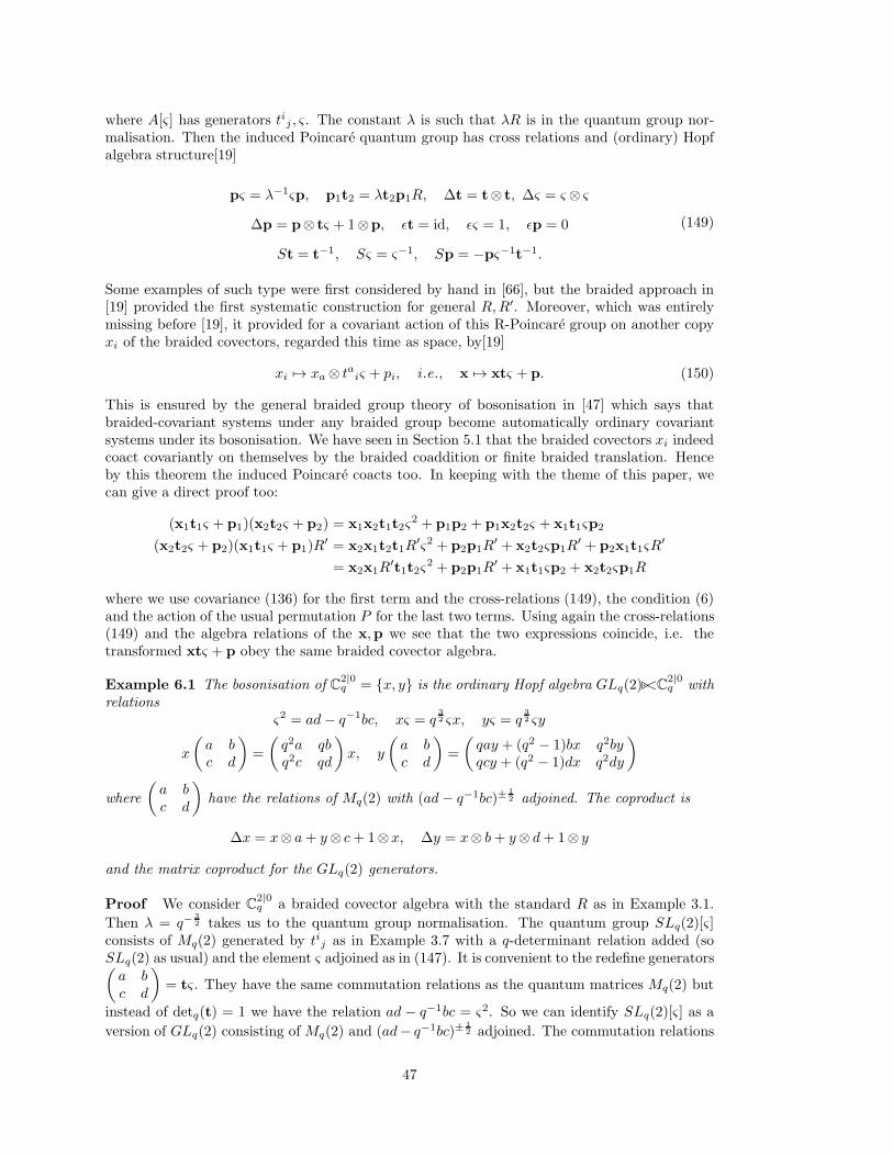
where A[ς ] has generators tij , ς . The constant λ is such that λR is in the quantum group nor-malisation. Then the induced Poincare quantum group has cross relations and (ordinary) Hopfalgebra structure[19]
pς = λ−1ςp, p1t2 = λt2p1R, ∆t = t⊗ t, ∆ς = ς ⊗ ς
∆p = p⊗ tς + 1⊗p, ǫt = id, ǫς = 1, ǫp = 0
St = t−1, Sς = ς−1, Sp = −pς−1t−1.
(149)
Some examples of such type were first considered by hand in [66], but the braided approach in[19] provided the first systematic construction for general R,R′. Moreover, which was entirelymissing before [19], it provided for a covariant action of this R-Poincare group on another copyxi of the braided covectors, regarded this time as space, by[19]
xi 7→ xa⊗ taiς + pi, i .e., x 7→ xtς + p. (150)
This is ensured by the general braided group theory of bosonisation in [47] which says thatbraided-covariant systems under any braided group become automatically ordinary covariantsystems under its bosonisation. We have seen in Section 5.1 that the braided covectors xi indeedcoact covariantly on themselves by the braided coaddition or finite braided translation. Henceby this theorem the induced Poincare coacts too. In keeping with the theme of this paper, wecan give a direct proof too:
(x1t1ς + p1)(x2t2ς + p2) = x1x2t1t2ς2 + p1p2 + p1x2t2ς + x1t1ςp2
(x2t2ς + p2)(x1t1ς + p1)R′ = x2x1t2t1R
′ς2 + p2p1R′ + x2t2ςp1R
′ + p2x1t1ςR′
= x2x1R′t1t2ς
2 + p2p1R′ + x1t1ςp2 + x2t2ςp1R
where we use covariance (136) for the first term and the cross-relations (149), the condition (6)and the action of the usual permutation P for the last two terms. Using again the cross-relations(149) and the algebra relations of the x,p we see that the two expressions coincide, i.e. thetransformed xtς + p obey the same braided covector algebra.
Example 6.1 The bosonisation of C2|0q = x, y is the ordinary Hopf algebra GLq(2)·⊲<C
2|0q with
relationsς2 = ad− q−1bc, xς = q
32 ςx, yς = q
32 ςy
x
(a b
c d
)=
(q2a qb
q2c qd
)x, y
(a b
c d
)=
(qay + (q2 − 1)bx q2by
qcy + (q2 − 1)dx q2dy
)
where
(a b
c d
)have the relations of Mq(2) with (ad− q−1bc)±
12 adjoined. The coproduct is
∆x = x⊗ a+ y⊗ c+ 1⊗x, ∆y = x⊗ b+ y⊗ d+ 1⊗ y
and the matrix coproduct for the GLq(2) generators.
Proof We consider C2|0q a braided covector algebra with the standard R as in Example 3.1.
Then λ = q−32 takes us to the quantum group normalisation. The quantum group SLq(2)[ς ]
consists of Mq(2) generated by tij as in Example 3.7 with a q-determinant relation added (soSLq(2) as usual) and the element ς adjoined as in (147). It is convenient to the redefine generators(a b
c d
)= tς . They have the same commutation relations as the quantum matrices Mq(2) but
instead of detq(t) = 1 we have the relation ad − q−1bc = ς2. So we can identify SLq(2)[ς ] as a
version of GLq(2) consisting of Mq(2) and (ad− q−1bc)±12 adjoined. The commutation relations
47

are then obtained from (149) using the explicit form of R. The coaction and corresponding
coproduct are given by
(a b
c d
)acting on (x, y) from the right as a matrix. ⊔⊓
This is a more or less well-known example and in the general family in [66] and elsewhere,but demonstrates the kind of structure one gets. From [19] we know that it necessarily coacts
covariantly on C2|0q by matrix multiplication and translation (150). Moreover, the braided ap-
proach allows us to bosonise all the other braided covector algebras in this paper just as welland obtain their natural induced ‘Poincare’ quantum groups and their coactions.
For example, when R is Hecke, we can apply the bosonisation to the additive braided groupsA(R), A(R) and B(R) just as well. We just use R,R′ from (27), (22), (36) respectively. ThePoincare groups consist of adjoining the Lorentz generators tIJ obtained from A(R). We canalso give a spinorial or matrix version using the quantum symmetry in the matrix form, as givenfor A(R) and B(R) in (139) and (141) respectively. In these cases we chose the quantum groupnormalisation constant λ such that A(R) has a quotient dual-quasitriangular Hopf algebra Aand from two copies of this we build A⊗A as the quantum covariance of A(R) and A⊲⊳A as thequantum covariance of B(R). We use for the latter the ⊲⊳ construction introduced by the authorand making use of the dual universal R-matrix R of A, see [19, Sec. 4]. In both cases we thenadjoin ς .
The R-matrix form of the induced Poincare quantum group (A⊗A)[ς ]·⊲<A(R) then has crossrelations and coproduct [25]
p1t2 = λt2p1R, p1s2 = s2λ−1R−1p1, pς = λ−2ςp
∆pij = pab⊗(Ssia)t
bjς + 1⊗ pij , i .e., ∆p = p⊗ s−1( )tς + 1⊗p
(151)
where the indices of p have to be inserted into the space. There is also a counit ǫp = 0 andantipode. The standard R-matrix put into these formulae provides the 4-dimensional q-Euclideanspace Poincare group appropriate to the q-Euclidean space algebra in Section 7.1 below.
The R-matrix form of the induced Poincare group (A⊲⊳A)[ς ]·⊲<B(R) has the cross-relationsand coproduct[67]
p1t2 = λ2t2R21p1R, p1s2 = s2R−1p1R, pς = λ−2ςp
∆p = p⊗ s−1( )tς + 1⊗p
(152)
in a similar way. There is also a counit ǫp = 0 and antipode. The standard R-matrix inserted intothese formulae gives us the q-Minkowski space Poincare group appropriate to the q-Minkowskialgebra in Section 7.2. Of course, our constructions (151)–(152) are quite general and not limitedto the standard R-matrix.
We conclude here by mentioning that also in [19] was given the corresponding Poincareenveloping algebra-type quantum group for the general construction (149). We give it in termsof the l± generators of Uq(g) in [22]. One can also use it for non-standard quantum envelopingalgebras when the universal R-matrix is known. This enveloping algebra is our ‘Lorentz orrotation’ algebra and all our constructions are covariant under its action (rather than coactionas before). First we extend Uq(g) by adjoining an infinitesimal scaling central generator ξ dualto the finite dilaton ς ,
∆ξ = ξ⊗ 1 + 1⊗ ξ, Rξ = λ−ξ⊗ ξ, 〈ς, ξ〉 = 1, or 〈ς, λξ〉 = λ (153)
We use its quantum line universal R-matrix[68]. The universal R-matrix of the extension ofUq(g) is its usual one[63][69] times this Rξ. We focus on braided vectors pi (say) as momentum
48

generators covariant under this extension. Bosonisation proceeds using the general theorem in[47] and gives the cross relations and Hopf structure [19]
λξpλ−ξ = λ−1p, l+1 p2 = λ−1R−121 p2l
+1 , l−1 p2 = λRp2l
−1
∆p = p⊗ 1 + l−λξ ⊗p, ǫp = 0, Sp = −λ−ξSl−p(154)
and a covariant action on braided covectors xi by
l+2 ⊲x1 = x1λR, l−2 ⊲x1 = x1λ−1R−1
21 , λξ⊲x = λ−1x, pi⊲xj = δij . (155)
The action of pi on products is according to the coproduct and is equivalent to a version (insome other conventions) of the braided-Leibniz rule (80) for braided derivatives. We can just aseasily give the enveloping algebra form of the matrix Poincare groups (151)–(152) by the sametechniques. See [25] for the action of the l± in these cases. We note that there are many otherapplications too of the bosonisation theory. See [70][71] for recent applications in connectionwith the differential calculus and Koszul complex of Uq(g).
7 q-Deformed spacetime
At various points in our tour of braided geometry we have mentioned that the examples Mq(2)and BMq(2) make natural q-Euclidean and q-Minkowski spaces when q is real. We just haveto specialise our general A(R) and B(R) constructions to the case of R given by the standardquantum plane or Jones polynomial R-matrix in the Hecke normalisation. We have seen abovemany results about these general algebras, all of which constitutes the braided approach to q-spacetime due to the author[11][27][33][19][25] and U. Meyer[28][67]. Among other general results,there is a theory of quantum Wick rotation introduced in [25] which strictly connects A(R)and B(R) by an algebraic twisting construction. There is also a purely quantum isomorphismB(R)∼=U(L) where L is a braided-Lie algebra and U(L) its braided enveloping algebra[9]. Theseare among the more advanced results of braided geometry which were not able to cover here.
Many authors have considered what algebras should be taken as the q-deformation of Eu-clidean and Minkowski spaces. In the Euclidean case the braided geometry approach based onMq(2) is compatible with the N = 4 case of the theory of SOq(N)-covariant quantum planesin [22][50][51][72][73] and elsewhere. It has been taken quite far by Fiore, Weich and others. Inthe Minkowski case our approach based on the braided matrices BMq(2) is compatible with theapproach of Carow-Watamura, Schlieker, Scholl, Watamura, Wess, Zumino and others, based onthe idea of q-Minkowski space as a tensor product of two quantum planes, see [34][29][35] andelsewhere. The mathematical basis for this overlap is the homomorphism (43)–(44) introducedby the author in [27], though its significance was not appreciated until somewhat later when thetwo approaches began to converge [19]. The final details for this convergence were worked outin [67, Sec. 3] using the dual-universal R-matrix functional R on the q-Lorentz group.
In the following two sections we explain cleanly and simply how some of our various braidedgroup constructions look in the case of Mq(2) and BMq(2). Some comments about which wereknown before for these particular algebras and which were obtained as far as I know for the firsttime as examples of the braided approach are collected at the end of each section.
7.1 q-Euclidean space
The algebra Mq(2)
ba = qab, ca = q−1ac, da = ad, db = q−1bd dc = qcd
bc = cb+ (q − q−1)ad(156)
49
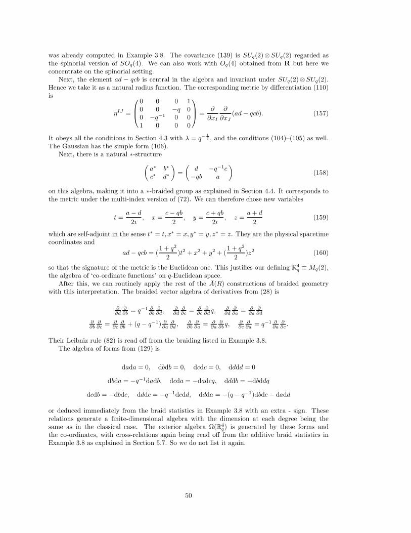
was already computed in Example 3.8. The covariance (139) is SUq(2)⊗SUq(2) regarded asthe spinorial version of SOq(4). We can also work with Oq(4) obtained from R but here weconcentrate on the spinorial setting.
Next, the element ad − qcb is central in the algebra and invariant under SUq(2)⊗SUq(2).Hence we take it as a natural radius function. The corresponding metric by differentiation (110)is
ηIJ =
0 0 0 10 0 −q 00 −q−1 0 01 0 0 0
=
∂
∂xI
∂
∂xJ(ad− qcb). (157)
It obeys all the conditions in Section 4.3 with λ = q−12 , and the conditions (104)–(105) as well.
The Gaussian has the simple form (106).Next, there is a natural ∗-structure
(a∗ b∗
c∗ d∗
)=
(d −q−1c
−qb a
)(158)
on this algebra, making it into a ∗-braided group as explained in Section 4.4. It corresponds tothe metric under the multi-index version of (72). We can therefore chose new variables
t =a− d
2ı, x =
c− qb
2, y =
c+ qb
2ı, z =
a+ d
2(159)
which are self-adjoint in the sense t∗ = t, x∗ = x, y∗ = y, z∗ = z. They are the physical spacetimecoordinates and
ad− qcb = (1 + q2
2)t2 + x2 + y2 + (
1 + q2
2)z2 (160)
so that the signature of the metric is the Euclidean one. This justifies our defining R4q ≡ Mq(2),
the algebra of ‘co-ordinate functions’ on q-Euclidean space.After this, we can routinely apply the rest of the A(R) constructions of braided geometry
with this interpretation. The braided vector algebra of derivatives from (28) is
∂∂d
∂∂b
= q−1 ∂∂b
∂∂d, ∂
∂d∂∂c
= ∂∂c
∂∂dq, ∂
∂d∂∂a
= ∂∂a
∂∂d
∂∂b
∂∂c
= ∂∂c
∂∂b
+ (q − q−1) ∂∂a
∂∂d, ∂
∂b∂∂a
= ∂∂a
∂∂bq, ∂
∂c∂∂a
= q−1 ∂∂a
∂∂c.
Their Leibniz rule (82) is read off from the braiding listed in Example 3.8.The algebra of forms from (129) is
dada = 0, dbdb = 0, dcdc = 0, dddd = 0
dbda = −q−1dadb, dcda = −dadcq, dddb = −dbddq
dcdb = −dbdc, dddc = −q−1dcdd, ddda = −(q − q−1)dbdc− dadd
or deduced immediately from the braid statistics in Example 3.8 with an extra - sign. Theserelations generate a finite-dimensional algebra with the dimension at each degree being thesame as in the classical case. The exterior algebra Ω(R4
q) is generated by these forms andthe co-ordinates, with cross-relations again being read off from the additive braid statistics inExample 3.8 as explained in Section 5.7. So we do not list it again.
50

The q-epsilon tensor from (119) is
ǫabcd = −ǫacbd = ǫadbc = −ǫadcb = ǫbcad = −ǫbcda = 1
−ǫcbad = ǫcbda = −ǫdabc = ǫdacb = −ǫdbca = ǫdcba = 1
ǫacdb = −ǫcdba = −ǫdcab = q, −ǫabdc = −ǫbacd = ǫbdca = ǫdbac = q−1
−ǫcadb = ǫcdab = q2, ǫbadc = −ǫbdac = q−2, −ǫadad = ǫdada = q − q−1.
We see that there are a few unexpected entries which are zero at q = 1.Finally, the Gaussian-weighted integral on degree two from Section 5.6 is Z[xIxJ ] = q−4ηIJ .
Its nonzero values on degree four are
Z[abcd] = −q−11, Z[acbd] = −q−7
Z[a2d2] = q2Z[b2c2] = q−2Z[c2b2] = Z[bc2b] = Z[cb2c] = q−10(q2 + 1)
along with the other cases implied by the relations in R4q. In terms of the spacetime coordinates
we have
Z[t2] = Z[z2] = 12q
−4, Z[x2] = Z[y2] = [2;q2]4 q−4
Z[t4] = Z[z4] = 3[2;q2]8 q−10, Z[x4] = Z[y4] = [3;q2]!
8 q−10
which shows a degree of spherical symmetry even in the noncommutative case.Our approach to q-Euclidean space is a useful R-matrix one introduced by the author in
[25] based on the formulae R21x1x2 = x2x1R etc., and making contact in the above specificexample with the N = 4 case of the approach based on SOq(N)-covariance. The general Ncould also be studied in our braided formalism as braided covector spaces. The differentials,epsilon tensor, Gaussian and integration in this family were known already [50][54][51][72] whileour braided approach adds such things as the braided addition law, the R-matrix form (151) ofthe Poincare group[25], its covariant action on the x, existence of the braided-exponential andseveral other results, including the quantum wick rotation by twisting[25] which systematicallyturns the above into the following results for q-Minkowski space. The specific relations (156)are in fact isomorphic in this example with usual quantum matrices Mq(2) which were alreadyanticipated as q-Euclidean space in [29, Appendix], with SUq(2)⊗SUq(2) as rotations.
7.2 q-Minkowski space
Finally we follow the same constructions as in the preceding section but now for the braidedmatrices B(R). It is ironic that the simplest example BMq(2) was the very first braided groupknown[11] but also turns out to be the most intersting for q-deformed physics. We have alreadygiven the algebra in Example 3.10 as
ba = q2ab, ca = q−2ac, da = ad, bc = cb+ (1− q−2)a(d− a)
db = bd+ (1− q−2)ab, cd = dc+ (1− q−2)ca.(161)
It has the covariance SUq(2)⊲⊳SUq(2) from (141). Its natural ∗-structure is not the usual tensorproduct one but involves also reversing the two SUq(2) factors. So these two SUq(2) are like theSUq(2) which physicists use when they work with SOq(1, 3) at the level of a complex Lie algebra.
This algebra has a nice braided-coproduct too corresponding to matrix multiplication asexplained in Section 3.3 and this at once picks out the braided determinant det(u) = ad−q2cb as
51
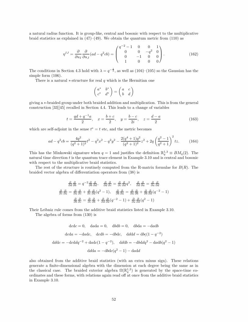
a natural radius function. It is group-like, central and bosonic with respect to the multiplicativebraid statistics as explained in (47)–(49). We obtain the quantum metric from (110) as
ηIJ =∂
∂uI
∂
∂uJ(ad− q2cb) =
q−2 − 1 0 0 10 0 −q2 00 −1 0 01 0 0 0
. (162)
The conditions in Section 4.3 hold with λ = q−12 , as well as (104)–(105) so the Gaussian has the
simple form (106).There is a natural ∗-structure for real q which is the Hermitian one
(a∗ b∗
c∗ d∗
)=
(a c
b d
)
giving a ∗-braided group under both braided addition and multiplication. This is from the generalconstruction [33][45] recalled in Section 4.4. This leads to a change of variables
t =qd+ q−1a
2, x =
b+ c
2, y =
b− c
2i, z =
d− a
2(163)
which are self-adjoint in the sense t∗ = t etc, and the metric becomes
ad− q2cb =4q2
(q2 + 1)2t2 − q2x2 − q2y2 −
2(q4 + 1)q2
(q2 + 1)2z2 + 2q
(q2 − 1
q2 + 1
)2
tz. (164)
This has the Minkowski signature when q = 1 and justifies the definition R1,3q ≡ BMq(2). The
natural time direction t is the quantum trace element in Example 3.10 and is central and bosonicwith respect to the multiplicative braid statistics.
The rest of the structure is routinely computed from the R-matrix formulae for B(R). Thebraided vector algebra of differentiation operators from (38) is
∂∂d
∂∂b
= q−2 ∂∂b
∂∂d, ∂
∂d∂∂c
= ∂∂c
∂∂dq2, ∂
∂d∂∂a
= ∂∂a
∂∂d
∂∂c
∂∂a
= ∂∂a
∂∂c
+ ∂∂c
∂∂d(q2 − 1), ∂
∂b∂∂a
= ∂∂a
∂∂b
+ ∂∂b
∂∂d
(q−2 − 1)
∂∂b
∂∂c
= ∂∂c
∂∂b
+ ∂∂d
∂∂d
(q−2 − 1) + ∂∂a
∂∂d
(q2 − 1)
Their Leibniz rule comes from the additive braid statistics listed in Example 3.10.The algebra of forms from (130) is
dcdc = 0, dada = 0, dbdb = 0, dbda = −dadb
dcda = −dadc, dcdb = −dbdc, dddd = dbc.(1− q−2)
dddc = −dcddq−2 + dadc(1− q−2), dddb = −dbddq2 − dadb(q2 − 1)
ddda = −dbdc(q2 − 1)− dadd
also obtained from the additive braid statistics (with an extra minus sign). These relationsgenerate a finite-dimensional algebra with the dimension at each degree being the same as inthe classical case. The braided exterior algebra Ω(R1,3
q ) is generated by the space-time co-ordinates and these forms, with relations again read off at once from the additive braid statisticsin Example 3.10.
52

The q-epsilon tensor from (119) is
ǫaddd = −ǫbdcd = −ǫdadd = ǫdbdc = ǫddad = −ǫddda = 1− q−2
−ǫadad = −ǫcdbd = ǫdada = ǫdcdb = q2 − 1
ǫabcd = −ǫacbd = ǫadbc = −ǫadcb = −ǫbacd = ǫbcad = −ǫbcda = ǫcabd = 1
−ǫcbad = ǫcbda = −ǫdabc = ǫdacb = ǫdbac = −ǫdbca = −ǫdcab = ǫdcba = 1
ǫacdb = −ǫcadb = ǫcdab = −ǫcdba = q2, −ǫabdc = ǫbadc = −ǫbdac = ǫbdca = q−2
and has even more nonzero elements than in the Euclidean case.Finally, the Gaussian-weighted integral on degree two from Section 5.6 is Z[uIuJ ] = q−4ηIJ .
Its nonzero values on degree four are
Z[abcd] = −q−12, Z[acbd] = −q−8, Z[bcd2] = −q−10(1− q−4)
Z[cbd2] = − 12Z[d
4] = −q−8(1− q−2)2, Z[ad3] = q−10(1 + 2q2)(1 − q−2)
Z[a2d2] = q4Z[b2c2] = Z[c2b2] = q2Z[bc2b] = q2Z[cb2c] = q−10(q2 + 1)
along with various other cases implied by the relations in R1,3q . In terms of spacetime coordinates
(163) we have
Z[t2] = [2;q2]4 q−4, Z[x2] = Z[y2] = Z[z2] = − [2;q2]
4 q−6
Z[z4] = 3[2;q2]8 q−12, Z[t4] = q4Z[x4] = q4Z[y4] = [3;q2]!
8 q−10.
We see that the Gaussian-weighted integral Z is quite similar to the Euclidean one in its values,except for the sign in the spacelike directions. We also note that the negative sign in the space-likedirections agrees with the sign obtained in physics by Wick rotation to make sense of Gaussianintegrals in Minkowski space.
We have developed q-Minkowski space cleanly and simply as a braided matrix R21u1Ru2 =u2R21u1R in the braided approach started in [11][26][27][33]. Because of the mapping (44) ourresults must necessarily recover in the standard 2 × 2 case the pioneering work in the spinorialapproach of [34][29][35] when one looks at the explicit algebra. On the other hand, our braidedformulae are always in a general R-matrix form; for example the spinorial form (152) for theq-Poincare group is a new result in [67] and can be contrasted with the explicit algebra relationsfound in [35] by other means. The role of SUq(2)⊲⊳SUq(2) as q-Lorentz group is due to [74][34]although its abstract structure is due to [61][19, Sec. 4], in the second of which the link withtwisting of the Euclidean rotation group was made precise. The algebra of differential forms[35]is not new but developed now in a constructive way from the braided coaddition[52]. The braidedapproach added principally such things as the coaddition itself[28], the comultiplication[11], theduality with braided vectors, the covariant action of the q-Poincare group on the spacetimegenerators[19], the existence of the braided exponential (though no very good formula for it), thebraided Gaussian and associated integral[44] even for this particular example. Further resultsin the braided approach are in [28] where a braided covector picture of both spacetime and theLorentz group is developed, and [53].
The braided approach also added the canonical isomorphism[9][5]
R1,3q ≡ BMq(2)∼=U(glq,2) (165)
which is a ‘purely quantum’ phenomenon since at q = 1 the left hand side becomes the commu-tative co-ordinates on Minkowski space while the right hand side becomes the non-commutative
53

enveloping algebra of su2⊕ u(1). This is obviously very interesting for particle physics since twofundamental ingredients of electroweak theory are unified by q-deformation. Under this quantum-geometry transformation the mass shell ad− q2cb = 1 in q-Minkowski space (the braided groupBSLq(2) in [11]) is isomorphic to the algebra of Uq(sl2)[26]. This also provided of course plentyof representations of the q-Minkowski space algebra by pulling back the usual finite-dimensional,q-boson or other favourite representations of the latter. A further application of braided-Liealgebras is in [75].
A Transmutation
Braided groups were first constructed (by the author) using a process of transmutation whichturns any quantum group containing a strict subquantum group (with universal R-matrix) into abraided one[12][13][17]. We give here an introduction to this theory. As in Section 6, we requirethe reader to be more familiar with advanced aspects of quantum group theory[60]. Of course, itis not necessary to know this construction if one just wants to work with braided groups alreadygiven to you, which is the line we have taken above.
The idea of transmutation is that the type of an algebraic object (the kind of object it is)is to some extent a matter of choice. As an example, we could start with a bosonic object(an ordinary quantum group) and consider the collection or category of things on which it(co)acts. This category might well be equivalent to some other category, such as the categoryof braided-coactions of a braided group. By applying braided-Tannaka-Krein reconstruction wecould reconstruct that braided-group[17]. The same principle applies quite generally, wheneverwe have a concept of ‘representation’ powerful enough to reconstruct the object being represented.We start with one type of object, take its representations, identify that category as equivalentto another category of representations of some other type of object, and reconstruct it. I callthis principle ‘transmutation’ because it changes the flavour of the object. It is a kind of Fouriertransform technique for mathematical concepts.
In our example, this idea becomes the following theorem[17][25]. If f : A → A1 is a Hopfalgebra homomorphism between two quantum groups, where A1 is dual-quasitriangular in thesense that there is a universal R-matrix functional Z : A1⊗A1 → C obeying (143) as in Section 6,then A can be transmuted by f into a braided group B as follows. It has the same linear spaceand coproduct as A but a new product, antipode and braiding[17][25]
a·b = a(2)b(2)Z(f((Sa(1))a(3))⊗ f(Sb(1))), Sa = Sa(2)Z(f((S2a(3))Sa(1))⊗ f(a(4)))
Ψ(a⊗ b) = b(2)⊗ a(2)Z(f((Sa(1))a(3))⊗ f((Sb(1))b(3))).(166)
We are underlining the braided product and antipode here to distinguish them from the quantumgroup ones forA in terms of which they are given. This braided group lives in the braided categoryof objects covariant under A1, by the coaction
b 7→ b(2)⊗ f((Sb(1))b(3)) (167)
which induces the braiding Ψ via (145).If A has its own dual-quasitriangular structureR : A⊗A→ C obeying (143) then the product
of B is braided-quantum-commutative in the sense
Z(f(b(1))⊗ f(a(1)))R(a(2)⊗ b(2))Z(f(Sa(3))⊗ f(b(3)))a(4)Z(f(a(5))⊗ f(b(4)))·b(5)
= b(1)Z(f(b(2))⊗ f(a(1)))·a(2)R(a(3)⊗ b(3)) (168)
as one verifies easily from the definition of its product in (166) and the axioms (143) for Zand R. This expresses the theorem in [17] that B in this case is a braided-quantum group withbraided-universal R-matrix functional, the above being the braided version of the second of (143).
54

Finally, all of this applies just as well at the bialgebra level, if A does not have an antipode. Justreplace f S by f−1, the convolution-inverse of f which we can suppose instead[17].
This is the general theory of transmutation in function algebra form. We also gave it inenveloping algebra form[13]. As an immediate example, suppose there is a quantum grouphomomorphism f : A(R) → A(Z) sending tij to the matrix generator f ij say of A(Z). Thecondition for this is Rf1f2 = f2f1R which is just the same as our covariance assumption (136). Itimplies and is essentially equivalent[19] to the matrix condition
R12Z13Z23 = Z23Z13R12, R23Z13Z12 = Z12Z13R23 (169)
as explained in Section 6 when deriving (4). From the transmutation formula (166) and (144)we obtain a braided group B(R,Z) with product cf.[27]
uij = tij , uijukl = tabt
dlZ
iacdZ
bjkc, i .e., u = t, u1Zu2 = Zt1t2, etc. (170)
where we write the generators of B(R,Z) as u and use their product ·, while on the right weuse the original product of A(R). The braiding comes out as in (30) with Z in place of R andcorresponding braid-statistics Z−1u′
1Zu2 = u2Z−1u′
1Z for braided matrix comultiplication. Thebraided-quantum-commutativity (168) becomes the relations
Z21RZ−1u1Zu2 = u2Z21u1R (171)
which is also immediate by transmutation (170) of the FRT relations of A(R) as RZ−1u1Zu2 =Rt1t2 = t2t1R = Z−1
21 u2Z21u1R. We assume in the derivation that Z is regular so that inprinciple one has a quantum group with antipode f−1, but this vanishes from the final formulaeusing (146). We gave these explicit formulae in [11][27] for the case B(R) ≡ B(R,R), where wechecked everything directly from the matrix data as a self-contained example of a braided group.This case was emphasised because the abstract braided-universal R-matrix functional is the ratioof the universal R-matrix functionals of A(R), A(Z) and therefore trivial when R = Z, i.e. B(R)has been made totally ‘braided commutative’. In this extreme the quantum non-commutativityof A(R) is fully traded for braid-statistics of B(R) as a ‘classical’ but braided matrix. Anotherextreme is B(R, id) = A(R). Other cases of B(R,Z) are intermediate between these extremesbut their derivation and the direct check that they form a braided group follows in the same wayas for B(R). [15],[76] seem to be the first to explicitly study such algebras B(R,Z) and checkthem directly from (171), (169). More importantly, Hlavaty obtained some interesting examples,see [15]. One can obtain further examples in the context of quantum principle bundles[2] andquantum homogeneous spaces, where homomorphisms between two quantum groups, which areall we need, abound.
The transmutation theory tells of course not only that B(R,Z) is a braided group, but alsothat the representations of A(R) become automatically Z-braided representations of B(R,Z).This is the essence of transmutation, as explained above. To see how it works in the matrixsetting, transmutation tells us that whenever our braided covectors xi from Section 3.1 are A(R)-covariant under (139) the same linear map x → xu becomes a Z-braided coaction of B(R,Z).The A(R)-covariance becomes through the map f an A(Z)-covariance, and the Z-braiding of thexi with anything else is induced by this, e.g., Ψ(x1⊗x2) = x2⊗x1Z(f(t1)⊗ f(t2)) = x2⊗x1Z
and likewise Ψ(u1⊗x2) = x2Z−1⊗u1Z, being derived in the same was as we derived (39)–
(40) in Section 6.1. The braided-covariance under B(R,Z) has to work by the general theoryabove, but one can check it directly as x1u
′1x2u
′2 = x1x2Z
−1u′1Zu
′2 = x2x1R
′Z−1u′1Zu
′2 =
x2x1Z−121 u′
2Z21u′1R
′ = x2u′2x1u
′1R
′ where the third equality is the covariance assumption (136)in terms of u. Recall that this in turn implies and is essentially implied by (4). The diagonal caseZ = R of this theory is how we obtained the braided coactions of B(R) in [27] as described inSection 4.1 above. Also, if t has an antipode then so does u, which is how to obtain the braidedantipode on BSLq(2) in [11] from that of SLq(2). Indeed, all constructions for quantum groupshave braided parallels because of transmutation. Details of the above and some further resultsabout B(R,Z) from the point of view of transmutation will appear in [77].
55

To give some other simple examples of transmutation, we let G be an Abelian group, CG itsgroup algebra and β a bicharacter on G, i.e. a function on G × G such that β(g, ) and β( , g)are multiplicative for each g ∈ G. We know from [68] that any bicharacter on G defines a (dual)-quasitriangular structure Z(g, h) = β(g, h) extended linearly. So we have a dual quantum group.The idea to use bicharacters in this was introduced in [14][68] as a quasitriangular structureon the Hopf algebra C(G), which is equivalent. Transmutation was also covered there and weare just repeating it in the dual form for convenience of the reader. So any quantum group Amapping onto CG gets transmuted to a quantum braided group B with structure from (166).
Example A.1 cf[41] Let R be a matrix solution of the QYBE and let its indices i = 1, · · · , n beassigned a degree |i| ∈ G, where G is an Abelian group and such that R has G-degree zero in thesense
Rijkl = 0 for all |i| · |k| 6= |j| · |l|.
Then for any bicharacter β the quantum matrices A(R) have a corresponding transmutationB(R, β) with braided group structure
β(i, k)β(j, b)Riakbuajubl = β(j, l)β(b, i)ukbu
iaR
ajbl; Rij
kl ≡ R
ijklβ(j, l)
−1
β(i, j) ≡ β(|i|, |j|), ∆u = u⊗u, ǫu = id, Ψ(uij ⊗ ukl) = ukl⊗ u
ijβ(i,k)β(j,l)β(j,k)β(i,l) .
Proof This is immediate as an application of transmutation. The choice of G-degree | | andthe degree-zero condition give us precisely a homomorphism A(R) → CG by f(tij) = δij |i|. Itclearly maps the coproducts in the sense (f ⊗ f)∆ = ∆f where ∆g = g⊗ g and ∆t = t⊗ t, asrequired for a bialgebra homomorphism. The convolution-inverse is f−1(tij) = Sf(tij) = δij |i|
−1
using the group-inverse. The new product from (166) is just
uijukl = tabt
clZ(δ
ia|i|
−1δbj |j| ⊗ δkc|k|
−1) = tijtklβ(|i|
−1|j|, |k|−1) = tijtkl
β(i, k)
β(j, k). (172)
The braided-quantum commutation relations (168) reduce to the ones stated, where we havewritten them in terms of a matrix R obeying a β-version of the QYBE. The braided group livesin the category of CG-covariant algebras with coaction from (167)
uij 7→ uab⊗ f−1(tia)f(t
bj) = uij ⊗ |i|
−1 · |j| (173)
which then induces the braiding Ψ(uij ⊗ ukl) = ukl⊗ u
ijβ(|i|
−1|j|, |k|−1|l|) as shown. We alsohave all the theory of comodules too, automatically. Thus our braided covectors xi and vectorsvi from Section 3.1 have the coaction
xi → xa⊗ f(tai) = xi⊗ |i|, vi 7→ va⊗ f−1(tia) = vi⊗ |i|−1 (174)
and with the induced braiding Ψ(uij ⊗xk) = xk ⊗uijβ(|i|
−1|j|, |k|) = xk ⊗uijβ(j,k)β(i,k) etc. Their
usual A(R)-covariance becomes a braided-covariance under x→ xu etc., provided we rememberthese induced braid statistics. Note also that if t has an antipode (if we work with a Hopf algebraobtained from A(R)) then the corresponding u has a braided antipode (166) computed in thepresent setting. ⊔⊓
These simplest braided-quantum groups where the braiding is given by a C-number bichar-acter β are called C-statistical braided groups in [68]. Their construction is an elementary ap-plication of the author’s transmutation theory. On the other hand, to find interesting exam-ples and applications is rather more challenging. The very simplest example is the super casewhere G = Z2 and β = ±1 (this is the quantum group Z′
2 which is the hidden covariance ofsupersymmetry[13] as mentioned in Section 6.1). The above transmutation in this case becomes
56
the process of superisation studied by the author and M.J. Rodriguez-Plaza in [41] (in an equiva-
lent form). The next simplest is G = ZN and β(g, h) = e2πıgh
N in an additive notation [14][16][77].Here [41] and [14] use transmutation in the enveloping form while [77] uses the dual form as above.Further details of Example A.1, further results about B(R,Z) and some concrete examples will
appear in [77]. Another choice is G = Zn or C
n and β(~φ, ~ψ) = eı(~φ,~ψ) induced by an arbitrary
non-degenerate bilinear form, see [68, Sec. 3] where braided groups of such C-statistics wereintroduced and studied from a bosonisation point of view as a novel approach to quantisationof free fields. Following exactly our transmutation ideas from [11][27] there appeared recentlyin [78] some explicit examples Mq,µ(n) of the G = Zn type obtained by transmutation of theusual quantum matrices Mq(n). The underlying mathematics is not new (in view of the abovetransmutation theory) but these examples are nevertheless interesting because of a connectionwith statistical mechanical models in physics[78]. Finally, we note that braided-quantum groupshave as rich a theory as usual quantum groups on account of their braided-universal R-matrix,as developed in [13] by diagrammatic means. Recent results using such means are in [79].
References
[1] S. Majid. Reconstruction theorems and rational conformal field theories. Int. J. Mod. Phys.A, 6(24):4359–4374, 1991.
[2] T. Brzezinski and S. Majid. Quantum group gauge theory on quantum spaces. Commun.Math. Phys., 157:591–638, 1993.
[3] S. Majid. Beyond supersymmetry and quantum symmetry (an introduction to braidedgroups and braided matrices). In M-L. Ge and H.J. de Vega, editors, Quantum Groups,Integrable Statistical Models and Knot Theory, pages 231–282. World Sci., 1993.
[4] S. Majid. Braided geometry: A new approach to q-deformations. To appear in Proc. 1stCaribb. Spr. Sch., Guadeloupe, May 1993. CUP.
[5] S. Majid. Lie algebras and braided geometry. Adv. Appl. Clifford Algebras (Proc. Supl.),4:61–77, 1994.
[6] S. Majid. Foundations of Quantum Group Theory. To appear. Cambridge Univeristy Press.
[7] S. Majid. On q-regularization. Int. J. Mod. Phys. A, 5(24):4689–4696, 1990.
[8] S. Majid. Hopf algebras for physics at the Planck scale. J. Classical and Quantum Gravity,5:1587–1606, 1988.
[9] S. Majid. Quantum and braided Lie algebras. J. Geom. Phys., 13:307–356, 1994.
[10] S. Majid. Rank of quantum groups and braided groups in dual form. volume 1510 of Lec.Notes. in Math., pages 79–89. Springer, 1992.
[11] S. Majid. Examples of braided groups and braided matrices. J. Math. Phys., 32:3246–3253,1991.
[12] S. Majid. Braided groups and algebraic quantum field theories. Lett. Math. Phys., 22:167–176, 1991.
[13] S. Majid. Transmutation theory and rank for quantum braided groups. Math. Proc. Camb.Phil. Soc., 113:45–70, 1993.
[14] S. Majid. Anyonic quantum groups. In Z. Oziewicz et al, editor, Spinors, Twistors, Clif-ford Algebras and Quantum Deformations (Proc. of 2nd Max Born Symposium, Wroclaw,Poland, 1992), pages 327–336. Kluwer.
57

[15] L. Hlavaty. Quantized braided groups. J. Math. Phys, 35:2560–2569, 1994.
[16] S. Majid and M.J. Rodriguez-Plaza. Anyonic FRT construction (1994). To appear in Czech.J. Phys.
[17] S. Majid. Braided groups. J. Pure and Applied Algebra, 86:187–221, 1993.
[18] S. Majid and M.J. Rodriguez-Plaza. Random walk and the heat equation on superspaceand anyspace. J. Math. Phys., 35:3753–3769, 1994.
[19] S. Majid. Braided momentum in the q-Poincare group. J. Math. Phys., 34:2045–2058, 1993.
[20] S. Majid. Free braided differential calculus, braided binomial theorem and the braidedexponential map. J. Math. Phys., 34:4843–4856, 1993.
[21] H. C. Lee, M. Couture, and N.C. Schmeing. Connected knot polynomials. Preprint, 1988.
[22] L.D. Faddeev, N.Yu. Reshetikhin, and L.A. Takhtajan. Quantization of Lie groups and Liealgebras. Leningrad Math J., 1:193–225, 1990.
[23] S. Majid. On the addition of quantum matrices. J. Math. Phys., 35:2617–2633, 1994.
[24] Yu.I. Manin. Quantum groups and non - commutative geometry. Technical report, Centrede Recherches Math, Montreal, 1988.
[25] S. Majid. q-Euclidean space and quantum Wick rotation by twisting. J. Math. Phys.,35:5025–5034, 1994.
[26] S. Majid. Braided matrix structure of the Sklyanin algebra and of the quantum Lorentzgroup. Commun. Math. Phys., 156:607–638, 1993.
[27] S. Majid. Quantum and braided linear algebra. J. Math. Phys., 34:1176–1196, 1993.
[28] U. Meyer. q-Lorentz group and q-Minkowski space with both braided coaddition and q-spinordecomposition, July 1993. To appear in Commun. Math. Phys.
[29] U. Carow-Watamura, M. Schlieker, M. Scholl, and S. Watamura. Tensor representation ofthe quantum group SLq(2,C) and quantum Minkowski space. Z. Phys. C, 48:159, 1990.
[30] I.V. Cherednik. Theor. Mat. Phys., 61:55, 1984.
[31] P.P. Kulish and E.K. Sklyanin. Algebraic structure of the reflection equations. J. Phys. A,25:5963–5975, 1992.
[32] L. LeBruyn. Homological properties of braided matrices, 1993. To appear in J. Algebra.
[33] S. Majid. The quantum double as quantum mechanics. J. Geom. Phys., 13:169–202, 1994.
[34] U. Carow-Watamura, M. Schlieker, M. Scholl, and S. Watamura. A quantum Lorentz group.Int. J. Mod. Phys., 6:3081–3108, 1991.
[35] O. Ogievetsky, W.B. Schmidke, J. Wess, and B. Zumino. q-Deformed Poincare algebra.Commun. Math. Phys., 150:495–518, 1992.
[36] S. Majid and M. Markl. Glueing operation for R-matrices, quantum groups and link invari-ants of Hecke type, July 1993. To appear in Math. Proc. Camb. Phil. Soc.
[37] D.I. Gurevich. Algebraic aspects of the quantum Yang-Baxter equation. Leningrad Math.J., 2:801–828, 1991.
58

[38] W. Pusz and S.L. Woronowicz. Twisted second quantization. Rep. Math. Phys, 27:231,1989.
[39] J. Wess and B. Zumino. Covariant differential calculus on the quantum hyperplane. Proc.Supl. Nucl. Phys. B, 18B:302, 1990.
[40] A.A. Vladimirov. Coadditive differential complexes on quantum groups and quantum spaces.J. Phys. A, 27:4497–4504, 1994.
[41] S. Majid and M.J. Rodriguez-Plaza. Universal R-matrix for non-standard quantum groupand superization. Preprint, DAMTP/91-47, 1991.
[42] A.P. Isaev. Interrelations between quantum groups and reflection equation (braided) alge-bras. Dubna Preprint, 1994.
[43] V.V. Lyubashenko and A. Sudbery. Quantum supergroups of GL(n|m) type: Differentialforms, Koszul complexes and Berezinians. Preprint, 1993.
[44] A. Kempf and S. Majid. Algebraic q-integration and Fourier theory on quantum and braidedspaces, January 1994. To appear in J. Math. Phys.
[45] S. Majid. ∗-structures on braided spaces. Preprint, damtp/94-65, 1994.
[46] S.L. Woronowicz. Compact matrix pseudo groups. Commun. Math. Phys., 111:613–665,1987.
[47] S. Majid. Cross products by braided groups and bosonization. J. Algebra, 163:165–190,1994.
[48] A. Kempf. Quantum group-symmetric Fock-spaces and Bargmann-Fock representation.Lett. Math. Phys., 26:1–12, 1992.
[49] C. Chryssomalakos and B. Zumino. Translations, integrals and Fourier transforms in thequantum plane. Preprint, November, 1993.
[50] U. Carow-Watamura, M. Schlieker, and S. Watamura. SOq(N)-covariant differential calculuson quantum space and quantum deformation of the Schrodinger equation. Z. Phys. C,49:439–446, 1991.
[51] G. Fiore. The SOq(N,R)-symmetric harmonic oscillator on the quantum Euclidean spaceRNq and its Hilbert space structure. Int. J. Mod. Phys. A, 26:4679–4729, 1993.
[52] S. Majid. q-epsilon tensor for quantum and braided spaces. Preprint, Damtp/94-20, 1994.
[53] U. Meyer. Wave equations on q-Minkowski space. Preprint, DAMTP/94-10, 1994.
[54] G. Fiore. Quantum groups SOq(N), Spq(N) have q-determinants, too. J. Phys. A, pages3795–3802, 1994.
[55] S.L. Woronowicz. Differential calculus on compact matrix pseudogroups (quantum groups).Commun. Math. Phys., 122:125–170, 1989.
[56] A. Sudbery. The algebra of differential forms on a full matric bialgebra. Math. Proc. Camb.Phil. Soc., 114:111, 1993.
[57] J.A. De Azcarraga and F. Rodenas. Differential calculus on q-minkowski space. To appearin Proc. 30th Winter School of Theoretical Physics, Karpacz, Poland, February 1994.
[58] G. Maltsiniotis. Groupes quantiques et structures differentielles. C.R. Acad. Sci. Paris,Serie I, 311:831, 1990.
59

[59] M. Pillin. q-deformed relativistic wave equations. J. Math. Phys., 35:2804–2817, 1994.
[60] S. Majid. Quasitriangular Hopf algebras and Yang-Baxter equations. Int. J. Modern PhysicsA, 5(1):1–91, 1990.
[61] S. Majid. More examples of bicrossproduct and double cross product Hopf algebras. Isr. J.Math, 72:133–148, 1990.
[62] S. Majid. Quantum groups and quantum probability. In Quantum Probability and RelatedTopics VI (Proc. Trento, 1989), pages 333–358. World Sci.
[63] V.G. Drinfeld. Quantum groups. In A. Gleason, editor, Proceedings of the ICM, pages798–820, Rhode Island, 1987. AMS.
[64] S. Majid. Algebras and Hopf algebras in braided categories. volume 158 of Lec. Notes inPure and Appl. Math, pages 55–105. Marcel Dekker, 1994.
[65] A. Macfarlane and S. Majid. Spectrum generating quantum group of the harmonic oscillator.Int. J. Mod. Phys., 7(18):4377–4393, 1992.
[66] M. Schlieker, W. Weich, and R. Weixler. Inhomogeneous quantum groups. Z. Phys. C,53:79–82, 1992.
[67] S. Majid and U. Meyer. Braided matrix structure of q-Minkowski space and q-Poincaregroup. Z. Phys. C, 63:357–362, 1994.
[68] S. Majid. C-statistical quantum groups and Weyl algebras. J. Math. Phys., 33:3431–3444,1992.
[69] M. Jimbo. A q-difference analog of U(g) and the Yang-Baxter equation. Lett. Math. Phys.,10:63–69, 1985.
[70] M. Schlieker and B. Zumino. Braided hopf algebras and differential calculus. Preprint, 1994.
[71] B. Drabant. Braided supersymmetry and (co)-homology. Preprint, 1994.
[72] A. Hebecker and W. Weich. Free particle in q-deformed configuration space. Lett. Math.Phys., 26:245–258, 1992.
[73] W. Weich. Quantum mechanics with SOq(n)-symmetry. Preprint, 1994.
[74] P. Podles and S.L. Woronowicz. Quantum deformation of Lorentz group. Commun. Math.Phys, 130:381–431, 1990.
[75] S. Majid. Solutions of the Yang-Baxter equations from braided-Lie algebras and braidedgroups, 1993. To appear in J. Knot Th. Ram.
[76] D.M. Lu. Braided matrices A(R,F ). Commun. Alg., 22:3009–3013, 1994.
[77] S. Majid and M.J. Rodriguez-Plaza. Anyonic quantum matrices. In preparation.
[78] M. Couture and H.P. Levio. The general quantum linear supergroup and braid statistics.J. Phys. A, 27:2367–2388, 1994.
[79] Yu. N. Bespalov. Crossed modules and quantum groups in braided categories I,II. Preprints,1994.
60