introduction to bayesian statistics - wordpress.com · introduction to bayesian statistics wei wu,...
TRANSCRIPT

3/6/2017
1
Introduction to Bayesian Statistics
Wei Wu, The University of Southern Mississippi
March 7, 2017
COA 640 – Quantitative Fisheries Management
Bayesian inference• Bayes’ theorem
Posterior = likelihood*prior/normalizing constant
Posterior likelihood*prior
• Advantage of Bayesian inference
‐‐ simplicity of interpretation of the results
‐‐ being consistent and ability of leaning from previous knowledge
‐‐ estimating different sources of errors
‐‐ data assimilation is automatic and the data need not be at the same scale and time
)(
)()|()|(
BP
APABPBAP
)()|()(
)()|()|(
PdataP
yP
PyPyP
3/6/2017
2
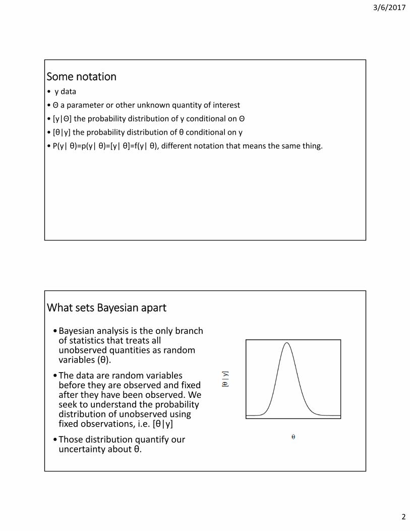
Some notation• y data
•Θ a parameter or other unknown quantity of interest
• [y|Θ] the probability distribution of y conditional on Θ
• [θ|y] the probability distribution of θ conditional on y
• P(y| θ)=p(y| θ)=[y| θ]=f(y| θ), different notation that means the same thing.
What sets Bayesian apart
•Bayesian analysis is the only branch of statistics that treats all unobserved quantities as random variables (θ).
•The data are random variables before they are observed and fixed after they have been observed. We seek to understand the probability distribution of unobserved using fixed observations, i.e. [θ|y]
•Those distribution quantify our uncertainty about θ.

3/6/2017
3
What sets Bayesian apart
One approach applies to many problems
‐ An unobservable state of interest, z
‐ A deterministic model of a process g(θ,x), controlling the state
‐ A model of the data
‐ Models of parameters
Prior information can be incorporated
Into the model for inference and
prediction
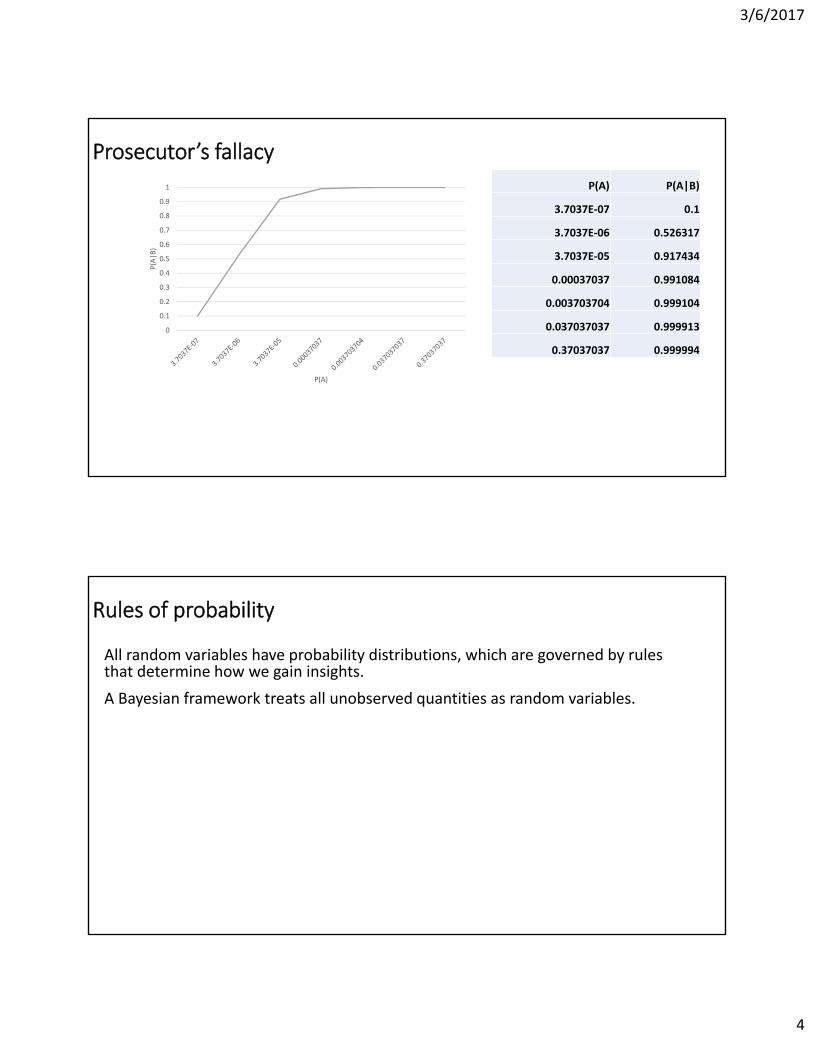
Prosecutor’s fallacy
Two sons of Sally Clark, a London Lawyer, died while very young about a year apart and both in mysterious circumstances.
Part of the evidence: The probability of two children dying of cot death in one family was extremely small (in court: one in 73 million).
A small p‐value does not necessarily mean that the alternative hypothesis is true.
A = Sally Clark murdered her two sons
P(A) = 3.7 x 10‐7 (one in 2.7 million)
B = Two sons died
P(B|A) = 1.0, P(B| ) = 3.33 x 10‐6 (one in 300,000)
P(A|B) =
A
1.0)107.31(1033.3107.30.1
107.30.1
)()|()()|(
)()|(
)(
)()|(767
7
APABPAPABP
APABP
BP
APABP
3/6/2017
4
Prosecutor’s fallacy
0
0.1
0.2
0.3
0.4
0.5
0.6
0.7
0.8
0.9
1
P(A|B)
P(A)
P(A) P(A|B)
3.7037E‐07 0.1
3.7037E‐06 0.526317
3.7037E‐05 0.917434
0.00037037 0.991084
0.003703704 0.999104
0.037037037 0.999913
0.37037037 0.999994
Rules of probability
All random variables have probability distributions, which are governed by rules that determine how we gain insights.
A Bayesian framework treats all unobserved quantities as random variables.

3/6/2017
5
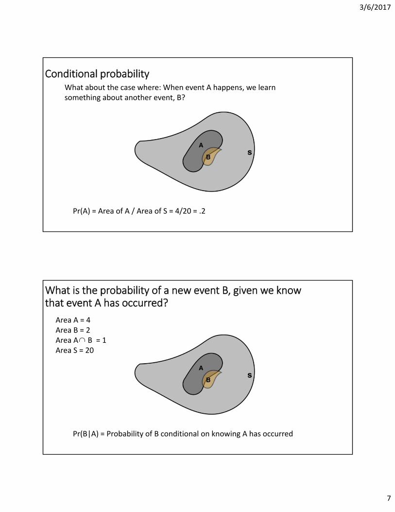
Sample space (S)
The set of all possible outcomes of an experiment.
The sample space has a specific area.
Events in S
Event A is a set of outcomes with a specific area.
The area of event A is less than the area of the sample space.

3/6/2017
6
What is the probability of event A?
Pr(A) = Area of A / Area of S
What is the probability of event A?
Area of A = 4Area of S = 20
Pr(A) = Area of A / Area of S = 4/20 = .2
3/6/2017
7
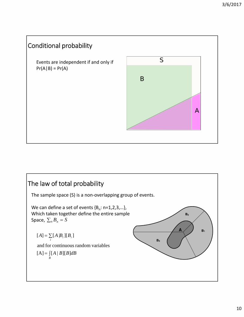
Conditional probabilityWhat about the case where: When event A happens, we learn something about another event, B?
Pr(A) = Area of A / Area of S = 4/20 = .2
What is the probability of a new event B, given we know that event A has occurred?
Area A = 4Area B = 2Area A B = 1 Area S = 20
Pr(B|A) = Probability of B conditional on knowing A has occurred
3/6/2017
8
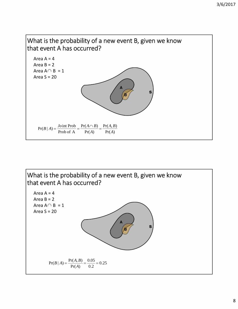
What is the probability of a new event B, given we know that event A has occurred?
Area A = 4Area B = 2Area A B = 1 Area S = 20
)Pr(
),Pr(
)Pr(
)Pr(
A of Prob
Prob int)|Pr(
A
BA
A
BAJoAB
What is the probability of a new event B, given we know that event A has occurred?
Area A = 4Area B = 2Area A B = 1 Area S = 20
25.02.0
05.0
)Pr(
),Pr()|Pr(
A
BAAB

3/6/2017
9
We can rearrange the equation
)Pr(
),Pr()|Pr(
A
BAAB
(2) A)Pr(A)|Pr(B B)Pr(A,
(1) ly equivalent and )Pr()|Pr(),Pr(
BBABA
Conditional probability
B)|Pr(AA)|Pr(B
True or false
3/6/2017
10
Conditional probability
Events are independent if and only ifPr(A|B) = Pr(A)
The law of total probability
The sample space (S) is a non‐overlapping group of events.
We can define a set of events {Bn: n=1,2,3,…},Which taken together define the entire sampleSpace, SBn n
B
iii
dBBBA
BBAA
]][|[[A]
variablesrandom continuousfor and
]][|[][

3/6/2017
11
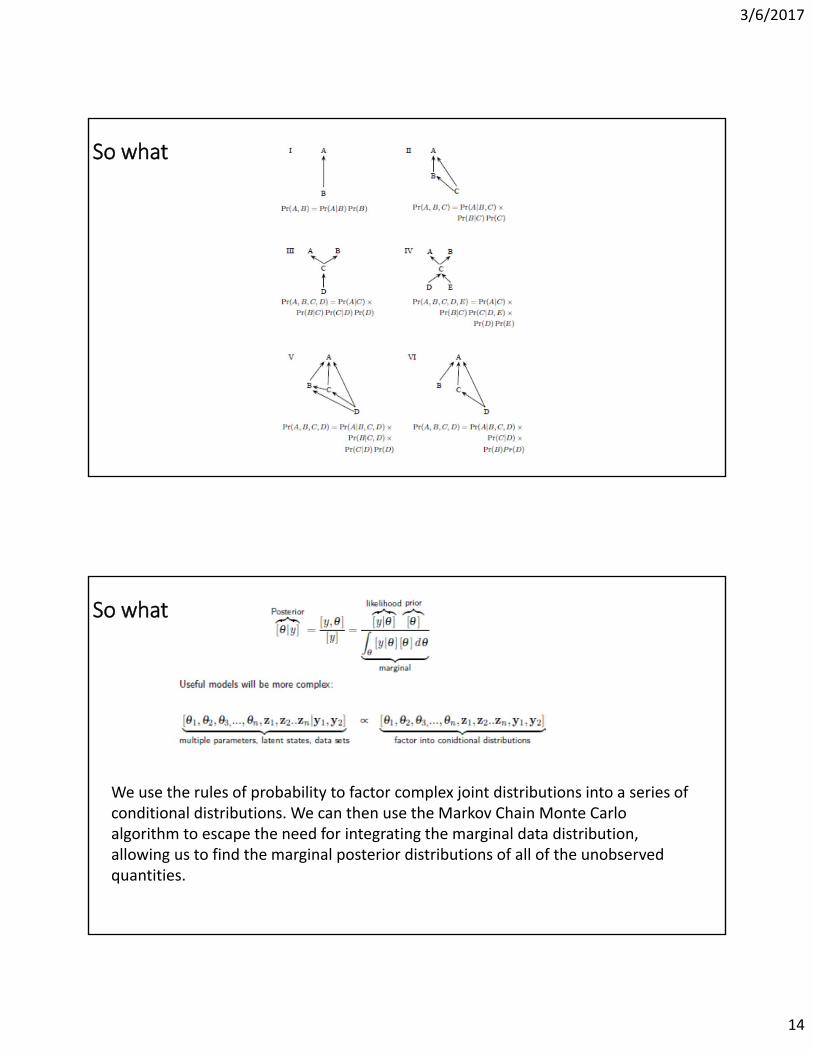
Factoring joint probabilities
The chain rule allows us to take complicated joint distributions of random variables and break them down into simpler conditional probabilities.
Conditional probabilities can be analyzed one at a time as if all other random variables are known and constant.
Factoring joint probabilities provide a usable graphical and mathematical foundation, which is critical for accomplishing the model specification step in the general modeling process.
Consider a Bayesian network (represented by a directed acyclic graph or DAG)
Bayesian networks specify how joint distributions are factored into conditional distributions using nodes to represent random variables (RV) and arrows to represent dependencies.
Notes at the heads of arrows must be on the left hand side of the conditioning symbols.
Nodes at the tails of arrows are on the right hand side of the conditioning symbols.
Any node at the tail of an arrow without an arrow leading into it must be expressed unconditionally.

3/6/2017
12
Factoring with DAGs
Pr(A,B) =
Factoring with DAGs
Pr(A,B) = Pr(A|B)Pr(B)

3/6/2017
13
Factoring with DAGs
Pr(A,B,C) = Pr(A|B,C)Pr(B|C)Pr(C)
So what
•What does this enable you to do? Review factoring joint distributions:
Remember from the basic laws of probability that
p(z1, z2) = p(z1|z2)p(z2)=p(z2|z1)p(z1)
This generalizes to:
z=(z1, z2, …, zn)
p(z1, z2, …, zn)=p(zn|zn‐1,…,z1)…p(z3|z2,z1)p(z2|z1)p(z1)
where the components zi may be scalars or subvectors of z and the sequence of their conditioning is arbitrary. This equation can be simplified using knowledge of independence.
3/6/2017
14
So what
So what
We use the rules of probability to factor complex joint distributions into a series of conditional distributions. We can then use the Markov Chain Monte Carlo algorithm to escape the need for integrating the marginal data distribution, allowing us to find the marginal posterior distributions of all of the unobserved quantities.

3/6/2017
15
The components of Bayes theorem
What is [y]
It follows that
continous are that parametersfor ]][|[
]][|[yy]|[
parameters valueddiscretefor ]][|[
]][|[yy]|[
parameters continuousfor ]][|[[y]
parameters discretefor ]][|[][
i
}{
i
}{
dy
y
dy
yy
i
ii
i
ii
i
i
3/6/2017
16
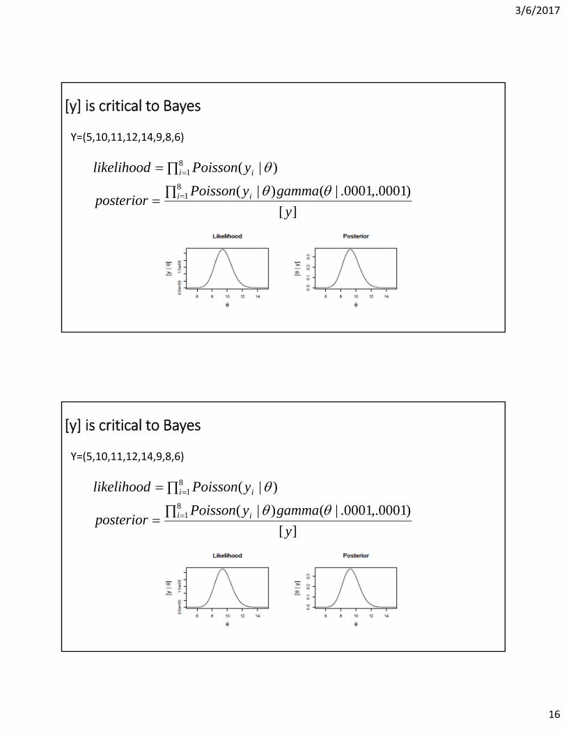
[y] is critical to Bayes
Y=(5,10,11,12,14,9,8,6)
][
)0001,.0001.|()|(
)|(8
1
81
y
gammayPoissonposterior
yPoissonlikelihood
ii
ii
[y] is critical to Bayes
Y=(5,10,11,12,14,9,8,6)
][
)0001,.0001.|()|(
)|(8
1
81
y
gammayPoissonposterior
yPoissonlikelihood
ii
ii

3/6/2017
17
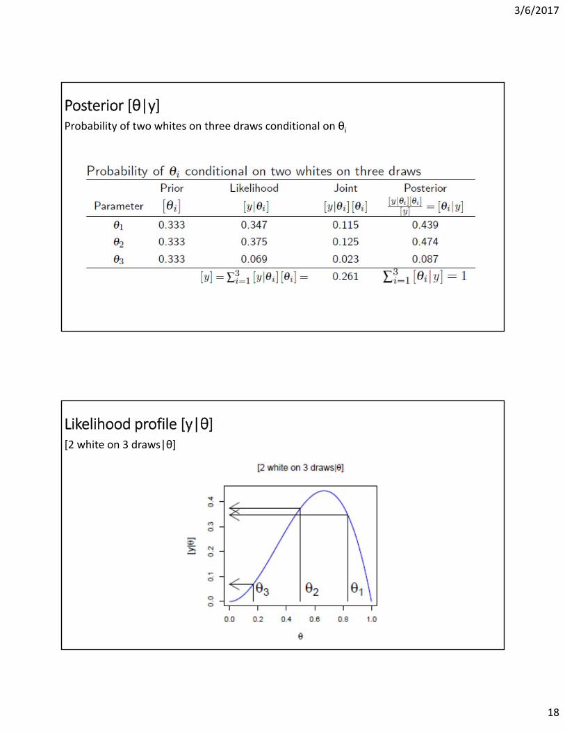
Probability [y|θ]Θ is known as to be ½. Probability of number of whites conditional on three draws
yny ppy
npnyp
)1(),|(
Likelihood [y|θ]Probability of two whites on three draws conditional on θi
3/6/2017
18
Posterior [θ|y]Probability of two whites on three draws conditional on θi
Likelihood profile [y|θ][2 white on 3 draws|θ]

3/6/2017
19
Posterior distribution [θ|y][θ| 2 white on 3 draws]
The components of Bayes theorem

3/6/2017
20
The components of Bayes theorem
dy
yy
]][|[
]][|[]|[
The prior, [θ], can be informative or vague.

3/6/2017
21
dy
yy
]][|[
]][|[]|[
The likelihood (data distribution [y|θ])
dy
y
y
yy
]][|[
]][|[
][
],[]|[
The product of the prior and the likelihood, [y|θ][θ], is the joint distribution of the parameters and the data, [y,θ]
What is the maximum likelihood estimate of θ?
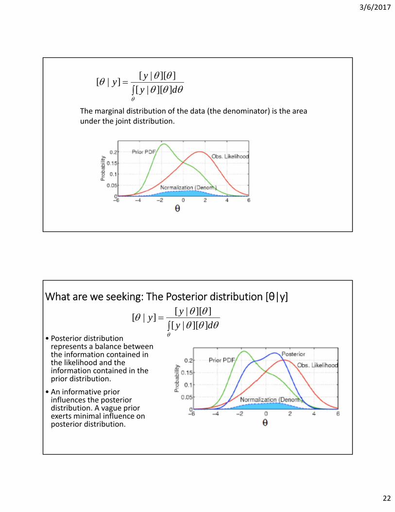
3/6/2017
22
dy
yy
]][|[
]][|[]|[
The marginal distribution of the data (the denominator) is the area under the joint distribution.
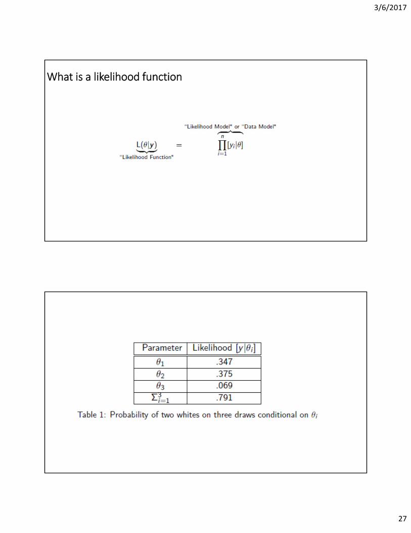
What are we seeking: The Posterior distribution [θ|y]
• Posterior distribution represents a balance between the information contained in the likelihood and the information contained in the prior distribution.
• An informative prior influences the posterior distribution. A vague prior exerts minimal influence on posterior distribution.
dy
yy
]][|[
]][|[]|[

3/6/2017
23
More on Likelihood
Likelihood forms the fundamental link between models and data in a Bayesian framework. In addition, maximum likelihood is a widely used alternative to Bayesian methods for estimating parameters insocio‐ecological models.
‐Hobbs and Hooten 2015

3/6/2017
24
Probability functions
For a discrete random variable, Y, the probability that the random variable Y takes on a specific value y is a probability function.
Tadpole example
You collect data on the number of tadpoles per volume of water in a pond. You observe 14 tadpoles in one litter sample.
You know the true average number of tadpoles per liter of water to b 23.
The probability of your data is
[yi|λ] = 0136.0!14
23 2314
e

3/6/2017
25
In this example, what did we treat as fixed and what did we treat as random?
In this example, what did we treat as fixed and what did we treat as random?
Parameter values (λ or θ) are fixed and the data (y) are random.

3/6/2017
26
What if, instead, you want to know the likelihood of the parameter given the observed data
The evaluation can be accomplished using a likelihood function L(θ|y)
What is a likelihood function
L(θ|y) = [y|θ]
L(θ|y)=
n
iiy
1]|[
3/6/2017
27
What is a likelihood function
3/6/2017
28
Likelihood profile
Likelihood as a concept
• Likelihood is the [y|θ].

3/6/2017
29
Likelihood as a concept
• Likelihood is the [y|θ].• Likelihood is the chance of observing your data given θ.
Likelihood as a concept
• Likelihood is the [y|θ].• Likelihood is the chance of observing your data given θ.• Likelihood is the probability of observing your data
conditional on your hypothesis θ.
3/6/2017
30
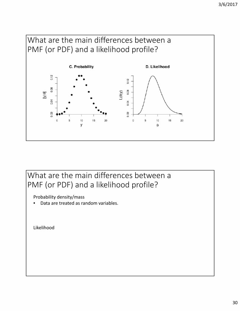
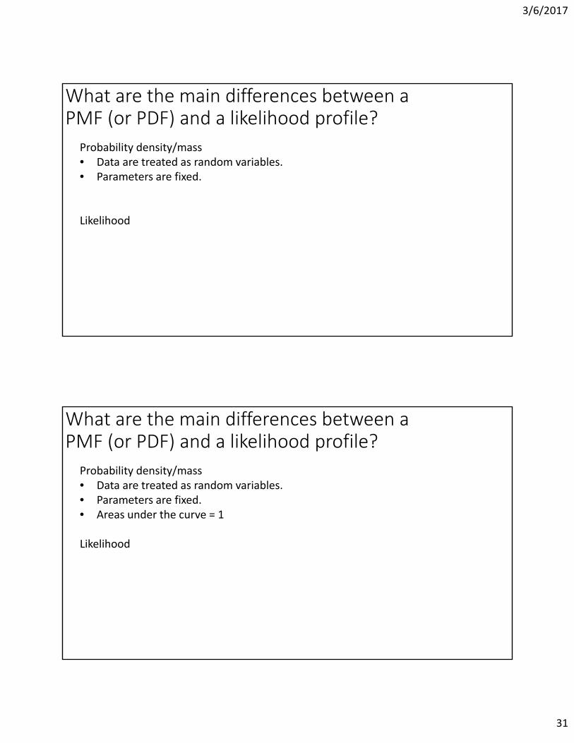
What are the main differences between a PMF (or PDF) and a likelihood profile?
What are the main differences between a PMF (or PDF) and a likelihood profile?
Probability density/mass• Data are treated as random variables.
Likelihood
3/6/2017
31
What are the main differences between a PMF (or PDF) and a likelihood profile?
Probability density/mass• Data are treated as random variables.• Parameters are fixed.
Likelihood
What are the main differences between a PMF (or PDF) and a likelihood profile?
Probability density/mass• Data are treated as random variables.• Parameters are fixed.• Areas under the curve = 1
Likelihood
3/6/2017
32
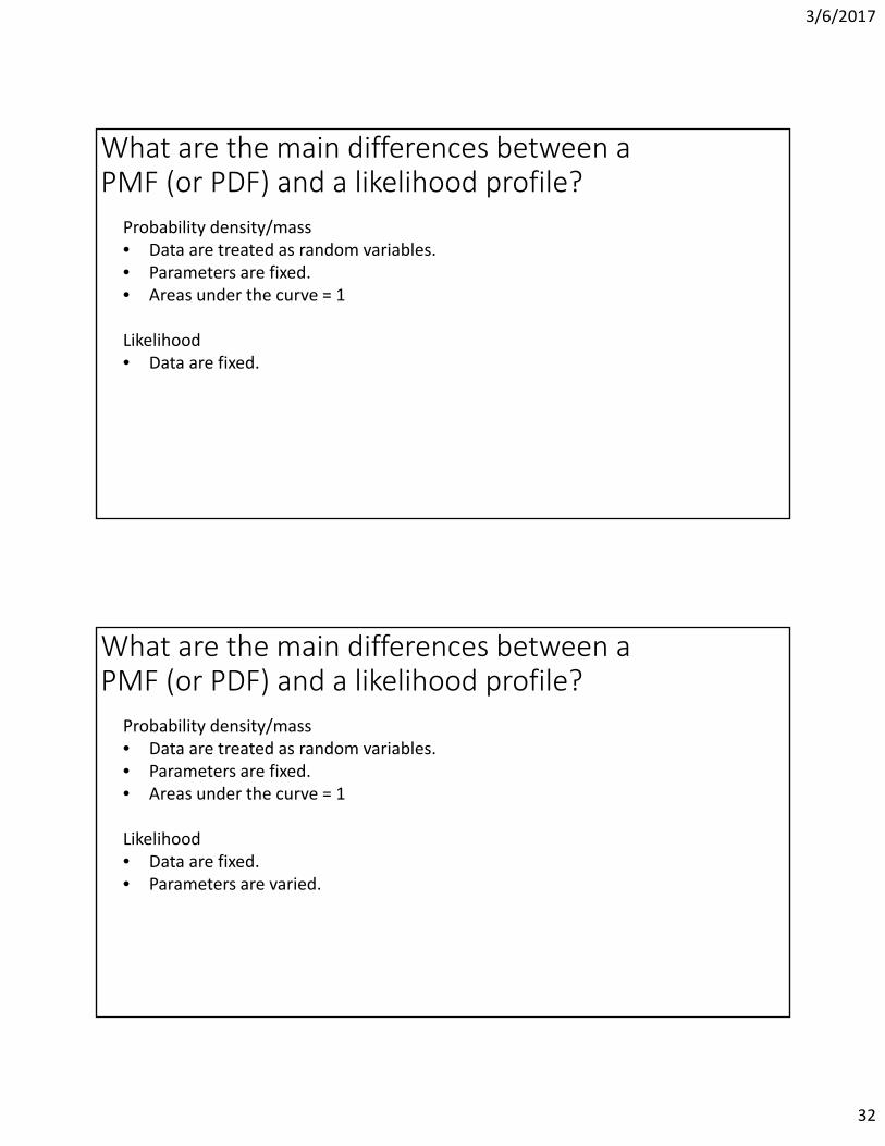
What are the main differences between a PMF (or PDF) and a likelihood profile?
Probability density/mass• Data are treated as random variables.• Parameters are fixed.• Areas under the curve = 1
Likelihood• Data are fixed.
What are the main differences between a PMF (or PDF) and a likelihood profile?
Probability density/mass• Data are treated as random variables.• Parameters are fixed.• Areas under the curve = 1
Likelihood• Data are fixed.• Parameters are varied.

3/6/2017
33
What are the main differences between a PMF (or PDF) and a likelihood profile?
Probability density/mass• Data are treated as random variables.• Parameters are fixed.• Areas under the curve = 1
Likelihood• Data are fixed.• Parameters are varied.• Areas under the curve ≠1.
What are the main differences between a PMF (or PDF) and a likelihood profile?
Probability density/mass• Data are treated as random variables.• Parameters are fixed.• Areas under the curve = 1
Likelihood• Data are fixed.• Parameters are varied.• Areas under the curve ≠1.• Y‐axis values are arbitrary and scalable.

3/6/2017
34
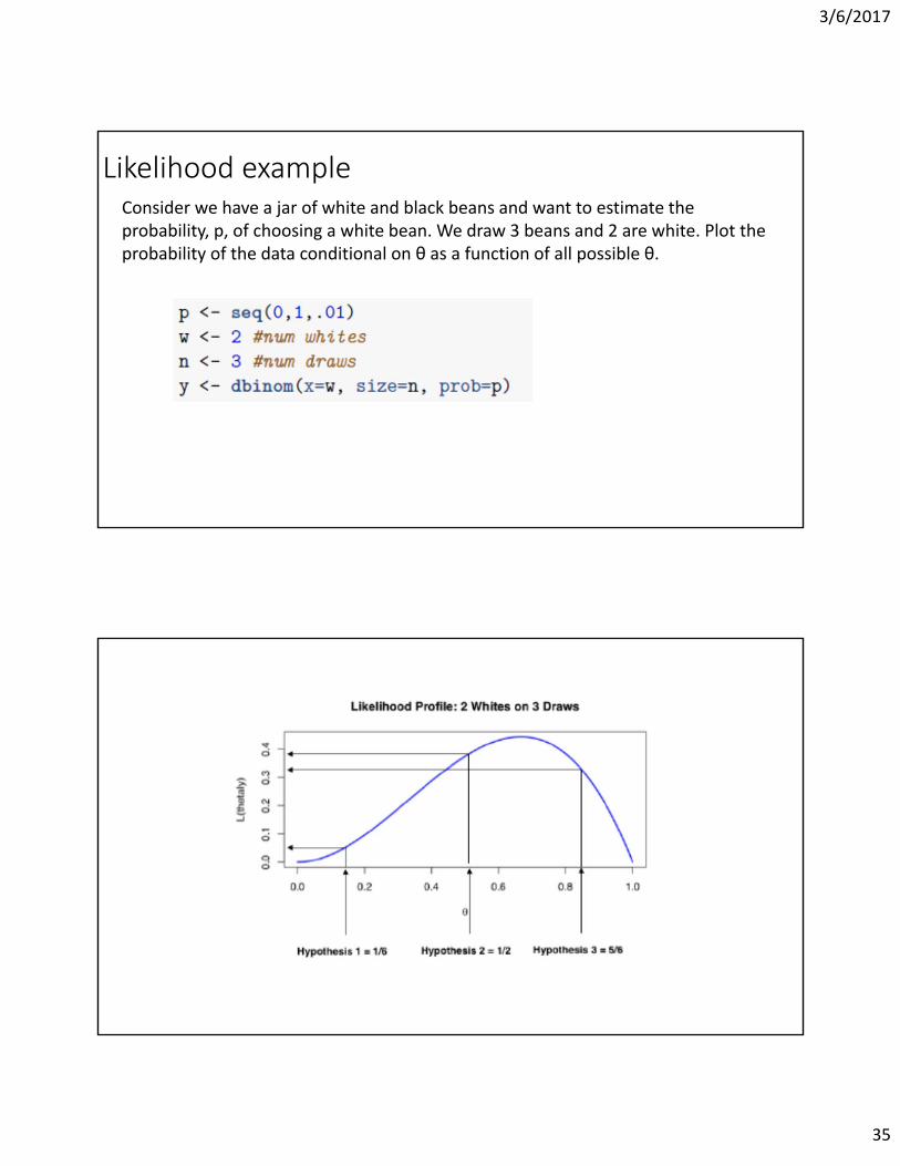
Understanding the likelihood profileWhat is the meaning of any one point on the likelihood profile curve?
Maximum likelihoodKnowing the likelihood of a specific parameter value doesn’t tell us anything useful in the absence of a comparison value. Therefore the evidence provided by data is expressed as the likelihood ratio.
Practically, we often want to know the value of parameter θ that has the maximum support in the data, which is the peak of the likelihood profile. This is the value of θthat maximizes the likelihood function.
]|[
]|[
)|(
)|(
2
1
2
1
y
y
yL
yL
3/6/2017
35
Likelihood exampleConsider we have a jar of white and black beans and want to estimate the probability, p, of choosing a white bean. We draw 3 beans and 2 are white. Plot the probability of the data conditional on θ as a function of all possible θ.

3/6/2017
36
Bayes theorem
• Likelihood: Links unobserved θ to observed y.
Bayes theorem
• Likelihood: Links unobserved θ to observed y.• Prior distribution: What is already known about θ.

3/6/2017
37
Bayes theorem
• Likelihood: Links unobserved θ to observed y.• Prior distribution: What is already known about θ.• Marginal distribution: the area under the joint distribution curve.
Serves to normalize the curve with respect to θ.
Bayes theorem
• Likelihood: Links unobserved θ to observed y.• Prior distribution: What is already known about θ.• Marginal distribution: the area under the joint distribution curve.
Serves to normalize the curve with respect to θ.• Posterior distribution: a true PDF.
3/6/2017
38
Prior distributions
Prior distributions can be informative, reflecting knowledge gained in previous research or they can be vague, reflecting a lack of information about θ before data are collected.
Prior distributions
• In special cases the posterior, [θ|y], has the same form as the prior, [θ].

3/6/2017
39
Prior distributions
• In special cases the posterior, [θ|y], has the same form as the prior, [θ].• In these cases, the prior and the posterior are said to be conjugate.
Prior distributions
• In special cases the posterior, [θ|y], has the same form as the prior, [θ].• In these cases, the prior and the posterior are said to be conjugate.• Conjugacy is important for two reasons:

3/6/2017
40
Prior distributions
• In special cases the posterior, [θ|y], has the same form as the prior, [θ].• In these cases, the prior is conjugate prior.• Conjugacy is important for two reasons:
‐ Conjugacy in simple cases minimizes computational work and, in more complicated cases, allow us to break down calculations into management units.
Prior distributions
• In special cases the posterior, [θ|y], has the same form as the prior, [θ].• In these cases, the prior and the posterior are said to be conjugate.• Conjugacy is important for two reasons:
‐ Conjugacy in simple cases minimizes computational work and, in more complicated cases, allow us to break down calculations into management units.
‐ Conjugacy plays an important role in Markov Chain Monte Carlo procedures.

3/6/2017
41
Conjugate priors
Just a bit more on priors
• There is no such thing as a truly non‐informative prior – only those that influences the posterior more (or less) than others.

3/6/2017
42
Just a bit more on priors
• There is no such thing as a truly non‐informative prior – only those that influences the posterior more (or less) than others.
• Informative priors can be justified and useful.
Just a bit more on priors
• There is no such thing as a truly non‐informative prior – only those that influences the posterior more (or less) than others.
• Informative priors can be justified and useful.• “Non‐informative:, vague, or flat priors are provisional starting points for
a Bayesian analysis.

3/6/2017
43
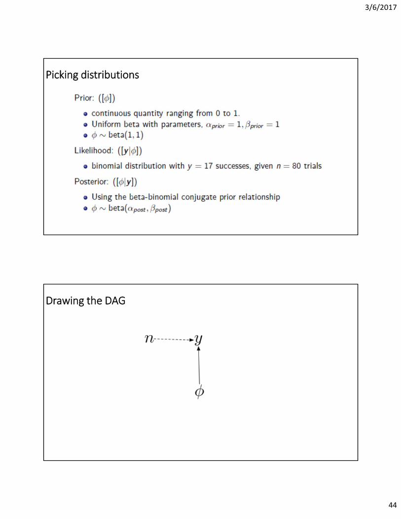
Example: Childhood asthma and PM
• You are studying the relationship between childhood asthma and industrial airborne PM.
• In one school, 17 of 80 students have been hospitalized for asthma‐related issues.
What distributions would you choose for the likelihood and prior?How would you draw the DAG?
Picking distributions
3/6/2017
44
Picking distributions
Drawing the DAG

3/6/2017
45
Writing out the full posterior
Posterior distribution parameters
This means you can

3/6/2017
46
This means you can
Literally calculate the parameters of the posterior distribution on the back of a hotel napkin.
Posterior distribution parameters
3/6/2017
47
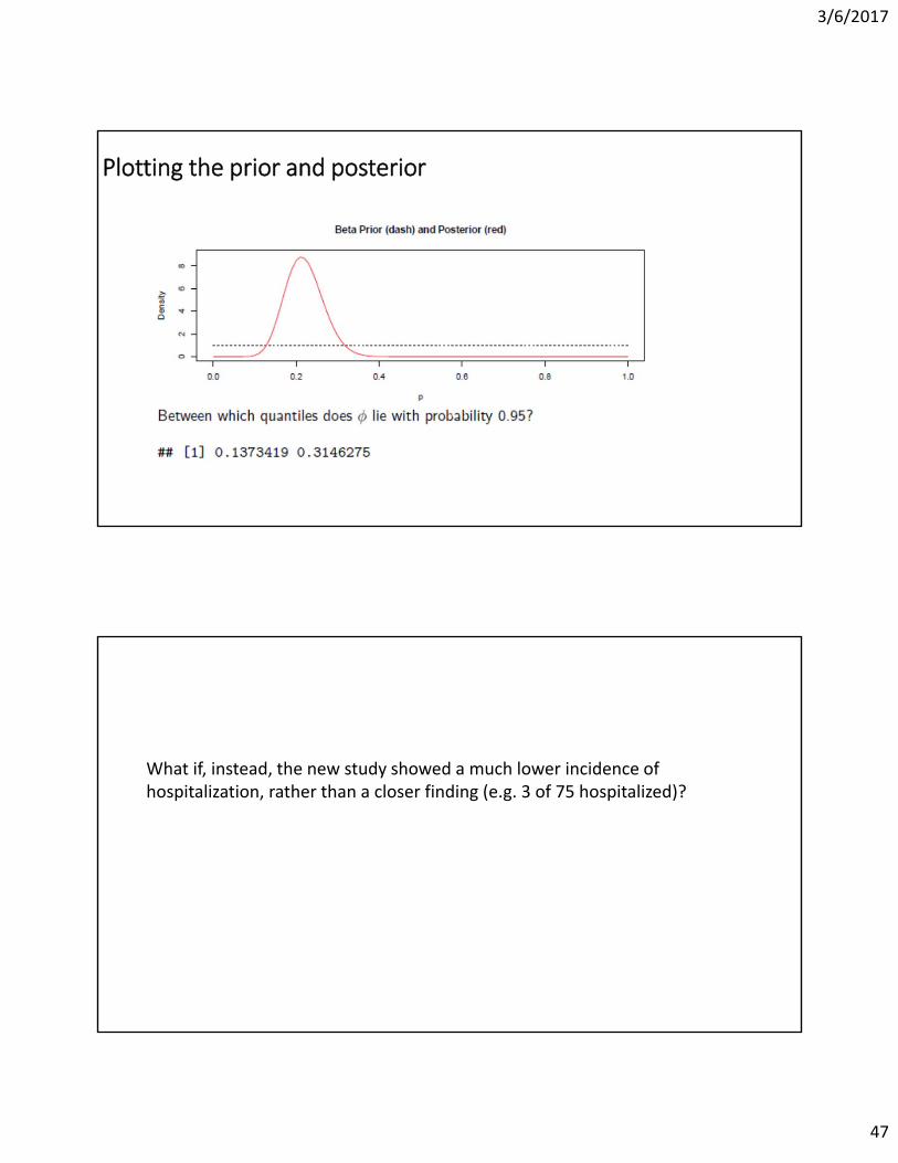
Plotting the prior and posterior
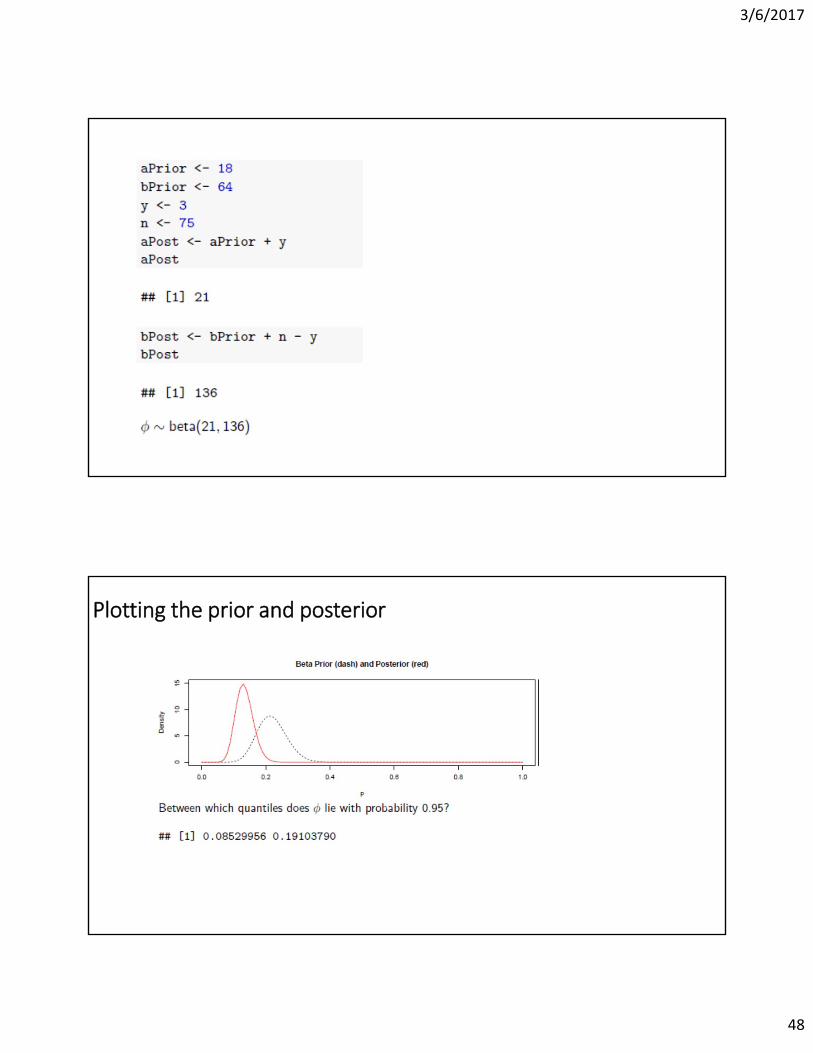
What if, instead, the new study showed a much lower incidence of hospitalization, rather than a closer finding (e.g. 3 of 75 hospitalized)?
3/6/2017
48
Plotting the prior and posterior
3/6/2017
49
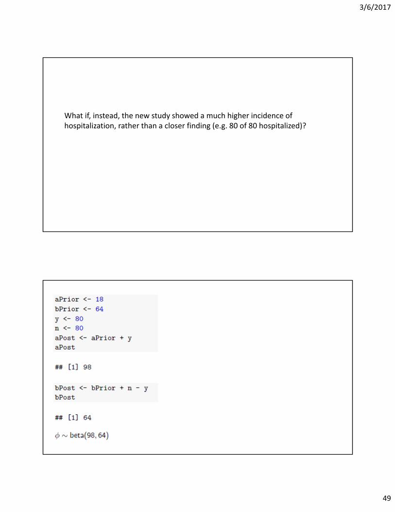
What if, instead, the new study showed a much higher incidence of hospitalization, rather than a closer finding (e.g. 80 of 80 hospitalized)?

3/6/2017
50
Plotting the prior and posterior
Exploring the role of new data (prior and data influence posteriors)
3/6/2017
51
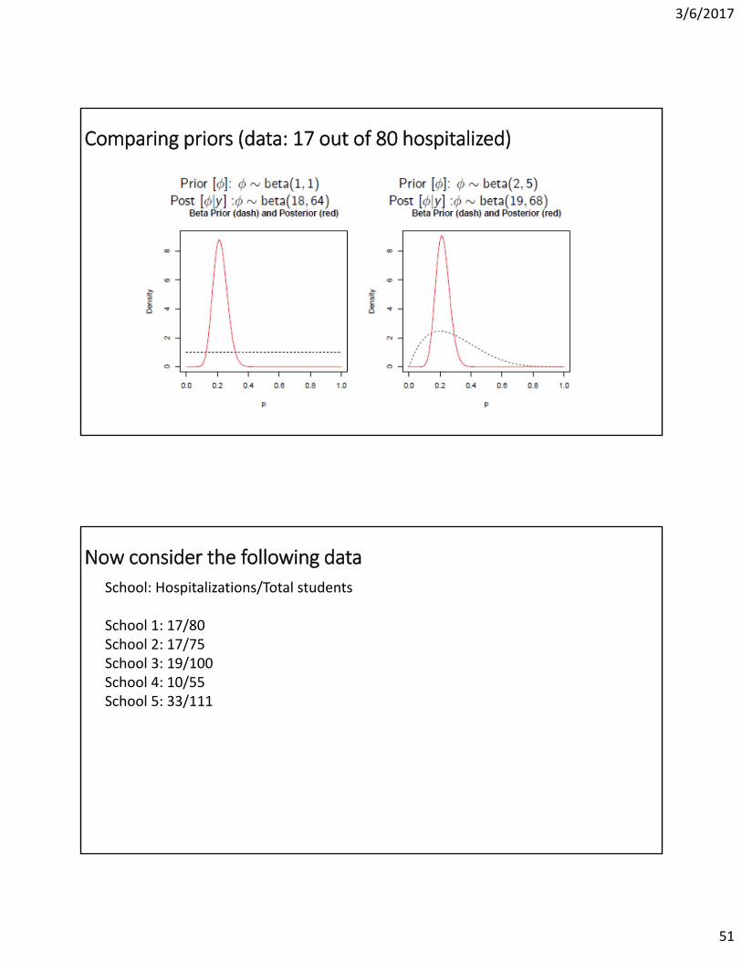
Comparing priors (data: 17 out of 80 hospitalized)
Now consider the following data
School: Hospitalizations/Total students
School 1: 17/80School 2: 17/75School 3: 19/100School 4: 10/55School 5: 33/111
3/6/2017
52
Now consider the following data
For a childhood asthma hospitalization model that, use the new data across schools, what is the DAG?
Full posterior
This is a hierarchical model because parameter, φ, is on both sides of the conditioning symbol.

3/6/2017
53
Things to remember
• This is no such a thing as a noninformative prior, but certain priors influence the posterior distribution more than others.
Things to remember
• This is no such a thing as a noninformative prior, but certain priors influence the posterior distribution more than others.
• Informative priors, when properly justified, can be useful.
3/6/2017
54
Things to remember
• This is no such a thing as a noninformative prior, but certain priors influence the posterior distribution more than others.
• Informative priors, when properly justified, can be useful.• Strong data overwhelms a prior.
Role of priors in science
• Priors represent our current knowledge (or lack of current knowledge), which is updated with data.

3/6/2017
55
Role of priors in science
• Priors represent our current knowledge (or lack of current knowledge), which is updated with data.
• We encourage you to think of vague priors as a provisional starting point.
Review
The posterior distribution represents a balance between theinformation contained in the likelihood and the informationcontained in the prior distribution.
θ
An informative prior influences the posterior distribution. A vagueprior exerts minimal influence.

3/6/2017
56
Influence of data and prior information
beta(φ|y) =binomial(y|φ,n) beta(φ|αprior ,βprior )
[y]
αposterior = αprior + yβposterior = βprior + ny
gamma(λ |y) =∏4
i = 1 Poisson(yi |λ ) gamma(λ |αprior ,βprior )
[y]
αposterior = αprior + ∑4ii = 1 y
βposterior = βprior + n
Influence of data and prior information

3/6/2017
57
Why use informative priors?
A natural tool for synthesis and updating
• Speed convergence
• Reduce problemswith identifyability
• Allows estimation of quantities that wouldotherwise beinestimable
• Reduces problemswith sensitivity totransformation
A vague prior is a distribution with a range of uncertaintythat is clearly wider than the range of reasonable values fortheparameter (Gelman and Hill 2007:347).
Also called: diffuse, flat, automatic, nonsubjective, locallyuniform, objective, and, incorrectly,“non‐informative.”

3/6/2017
58
The MCMC algorithm
Allows us to find the marginal posterior distribution of each of the unknowns while avoiding any formal integration.
The essential idea of MCMC is that we can learn about the unknowns by making many random draws from their marginal posterior distributions.
We can think of MCMC as an algorithm that normalizes the likelihood profile weighted by prior.
We can also easily obtain posterior distributions of any quantity that is derived from the unknowns we estimate – enormous benefit of MCMC.
What are we doing in MCMC?
• The posterior distribution is unknown, but thelikelihood isknown as a likelihood profile and we knowthe priors.
• We want to accumulate many, many values thatrepresent the random samples in the simulated posterior distribution proportionate totheir probability.
• Chain: A sequence of values accumulated from random draws from the posterior distribution.
• MCMC generates these samples using the likelihood andthe priors to decide which samples to keep and which tothrow away.
• We can then use these samples to calculatestatisticsdescribing the distribution: means,medians, variances, credible intervals etc.

3/6/2017
59
What are we doing in MCMC
Algorithms for drawing samples from the posterior
1. Accept-reject samplers
1. Metropolis: requires a symmetric proposal distribution (e.g., normal, uniform)
2. Metropolis-Hastings: allows asymmetric proposal distributions(e.g., beta, gamma, lognormal)
2. Gibbs: accepts all proposals because they come directly fromthe posterior using conjugates.

3/6/2017
60
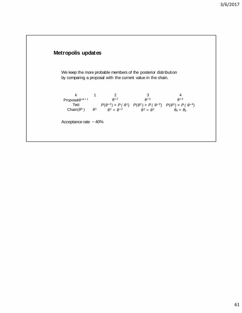
Metropolis updates
We keep the more probable members of the posterior distributionby comparing a proposal with the current value in the chain.
kProposalθ∗k + 1
Test Chain(θk )
1 2θ∗2
P(θ∗2) > P ( θ1 )θ2 = θ∗2θ1
Metropolis updates
We keep the more probable members of the posterior distributionby comparing a proposal with the current value in the chain.
kProposalθ∗k + 1
Test Chain(θk )
1 2θ∗2
P(θ∗2) > P ( θ1)θ2 = θ∗2
3θ∗3
P(θ2 ) > P ( θ∗3)θ3 = θ2θ1
3/6/2017
61
Metropolis updates
We keep the more probable members of the posterior distributionby comparing a proposal with the current value in the chain.
kProposalθ∗k + 1
Test Chain(θk )
1 2θ∗2
P(θ∗2) > P ( θ1)θ2 = θ∗2
3θ∗3
P(θ2 ) > P ( θ∗3)θ3 = θ2
4θ∗4
P(θ3 ) > P ( θ∗4)θ1 θ4 = θ3
Acceptance rate ~ 40%