introduction to basic economics...

APPENDIX

Introduction to BasicEconomics Concepts

This appendix serves as a very brief overview of some of the main economicsconcepts used throughout this book. If the reader has had an introductory orintermediate economics course before this (and the book aims at such a stu-dent), this material should serve as a quick reminder of the basic concepts.For the student who has never encountered economic thinking before, pleaseremember that entire books and one- to two-semester courses usually coverthe material that follows, and judge the adequacy of the coverage of thismaterial found here with mercy.

THE CONCEPT OF UTILITY AND DEMAND CURVESEconomists begin their study of human behavior by making what somewould consider a rash assumption, namely that every consumer has a stableset of preferences that allows comparison of different “bundles” of goods(taken here very broadly to mean goods and services produced in the marketor activities that might take place out of the market). These preferences arenormally represented as a “utility function” showing how additional amountsof each good increase total “well-being” or (in the usual term) “utility.” Econo-mists normally presume that “goods” continue to add utility as more areconsumed, so sometimes the “good” becomes the removal of a noxious sub-stance. For example, garbage removal may be the good rather than garbage.The list of possible goods is very large. Think about how many bar codes existfor all the stores in the world; each one describes a different good and this still

571

Z02_PHEL4570_04_SE_APP.QXD 1/15/09 12:40 PM Page 571

572 APPENDIX INTRODUCTION TO BASIC ECONOMICS CONCEPTS

misses items such as “watching a sunset” for which no bar code (yet) exists.To simplify the discussion, we usually abstract from the specific names ofthese goods and simply call them etc. Thus, the utility functionbecomes where N is the number of goods thatone might possibly wish to consider. For reasons of simplicity—includingour ability to diagram these concepts readily—economists often collapse thediscussion to two goods (which can then be pictured on a two-dimensionalgraph, as you will see shortly). This actually does not cause a great loss of pre-cision in thinking because these two goods can be one specific good (such aspopcorn or peanuts) and the other a “composite bundle” of all other goodsand services.

Economic thinking rests fundamentally on the premise that consumersmake choices to maximize their utility, limited by the amounts of goods thatthe consumer’s income can purchase. In more elaborate versions of thisproblem, income itself represents choices made by the consumer in the cur-rent period (how much to work versus how much to enjoy leisure) as well asthe cumulative effects of many past decisions (how much education to seek,how hard to study in classes of health economics, how much to save for thefuture). We assume that consumers not only know their preferences but alsohow to act to maximize their own utility. Although few economists believethat this literally occurs in every human choice, a very fruitful study ofhuman behavior emerges from this simple yet powerful paradigm.1

These types of decisions can be portrayed easily either in graphs or byusing the branch of mathematics known as calculus. The basic “problem” ofthe consumer is to maximize utility subject to a budget constraint,2 and thiscan be easily portrayed (in a simplified version) in a two-dimensional graph.In this graph, we focus on a specific good (say, ) and choices between thatgood and all other goods. Figure A.1 shows two key features about how goodsaffect utility. First, for any specified amount of adding more adds tototal utility but at a decreasing rate. This conforms to the simple idea that weeventually become “sated” in our consumption of a specific good. The for-mal statement of this says that we have positive but diminishing marginal(or incremental) utility for any specific good such as (The same is saidX1 .

X1Xother ,

X1

Utility = U1X1 , X2 , Á XN2X1 , X2 , Á

1A classic discussion of these issues is found in Milton Friedman’s Essays in Positive Economics(1966).2This type of problem commonly uses an approach devised by mathematician Joseph-LouisLagrange, known (not by coincidence) as Lagrange multipliers. Lagrange is usually consideredto be French, but he was born in Turin, Italy, and wrote his famous essay on finding maximaand minima in 1755 in Italian at age 19, probably younger than almost every reader of thistextbook! (What had you done by age 19?)


THE CONCEPT OF UTILITY AND DEMAND CURVES 573

Utility

X1

U1

U2

X1f

X1eX1

c

X1d

X1bX1

a

D E F

A B C

Xother = 10

Xother = 9

Xother = 8

(a)

X1

Xother

X1a A

B

C

U1

D

E

F

U2

(b)

FIGURE A.1

symmetrically for because it represents a bundle of all other goods andservices. Indeed, any one of those could be pulled out and treated similarly to

) The other key feature of Figure A.1(a) shows that similarly shapedcurves exist for each possible level of but utility is lower as the amountof falls so that these curves “nest” one under another as the amount of

falls.Now comes an important step: We take the information from the curves

in Figure A.1(a) and transform the same information into a different graph,one using and on the axes. (This is why we want to work only withtwo goods. Otherwise this becomes an n-dimensional graph that’s difficult ifnot impossible to draw for ) To see how this works, pick a specific levelof utility in Figure A.1(a) (say, ), and think about the combinations ofand that could create exactly Figure A.1(a) shows three possiblelevels of arbitrarily designated as 8, 9, and 10 (but they could be any-thing because we haven’t said in what units is measured). Points A, B,and C all have exactly the same level of utility but each has a differentcombination of and The graph of those points (and all others likethem if we’d drawn more curves in Figure A.1(a) for different amounts of

) creates an isoutility curve at utility level in Figure A.1(b).3 Morecommonly, economists call these indifference curves because the consumer isliterally indifferent to which of any combination of goods on each curve is

U1Xother

Xother .X1

1U12,Xother

Xother ,U1 .Xother

X1U1

n Ú 3.

XotherX1

Xother

Xother

Xother ,X1 .

Xother

3These come from the Greek word isos meaning “equal.”



best to consume.4 Points D, E, and F from Figure A.1(a) translate into a sepa-rate indifference curve in Figure A.1(b). We could create an extremelylarge number of such curves in Figure A.1(b) (an infinite number of them,actually) by picking specific levels of utility in Figure A.1(a) and graphing therelevant points over to Figure A.1(b). We usually draw only a few of suchcurves to symbolize the overall idea, and (as you will see in a moment), onlyone of them eventually matters—the highest one achievable with the budgetavailable to the consumer.

These curves are really no different than many maps you’ve often read.Weather maps, for example, either with curves or colors, show areas of thecountry with the same temperature. Meteorologists call these isothermalmaps, meaning “same temperature.” Topographical maps show lines of con-stant altitude, and anybody who’s ever used these maps soon becomes able tolook at them and figure out what the terrain that the map depicts looks like.

The next step allows us to move from the ephemeral world of utility(which we can’t really see or measure) to the concrete world of prices andquantities. Begin with (and slightly generalize) the graph in Figure A.1(b)and then think about how to add information about the consumer’s buyingpower, the “budget” available to buy goods and services. In the simplestmodel, the consumer’s income (I) is fixed at a specific level (say, ). InFigure A.2(a), this income appears as a downward-sloping straight line with aslope determined by the relative prices of and .5 The trick is to findthe highest possible level of utility (remember that the consumer is trying tomaximize utility within the constraint of the budget available), and it’s easy

XotherX1

I1

U2

4A personal note: The word indifferent has a specific meaning to economists not universallyshared by others. It refers to combinations of things that create the same utility. Early in mymarriage, my wife would sometimes ask me, “Do you want peas or corn with the meat loaftonight?” Because I’d just learned the concept of indifference in an economics class, I wouldrespond “I’m indifferent,” meaning “either would be fine.” Before I explained this conceptclearly, she heard instead “I don’t want either” as my message, and this came close to ruiningour marriage until I explained the underlying economic idea to her. I can now say “I’m indif-ferent” without having to call a marriage counselor.5To show why the budget line is a straight and downward-sloping line in this graph, begin withthe notion that all available income is spent on goods and purchased at prices of(for ) and (arbitrarily) a price of 1 for other goods. Thus Now we askwhat combinations of goods could exactly consume the total budget I. To do this, increase by a little bit and ask how much has to fall to keep within the budget. Adding one unit of

causes spending to increase by so the amount of has to fall by exactly to keeptotal spending the same. The constant-budget line in the graph with and on the axesthus has a slope of More generally, in a graph of versus the budget line will havea slope of -pj/pi .

Xj ,Xi-1/p1 .XotherX1

1/p1Xotherp1 ,X1

Xother

X1

I = p1X1 + Xother .X1

p1XotherX1


THE CONCEPT OF UTILITY AND DEMAND CURVES 575

to see that one does this by finding the highest possible indifference curvethat just touches the budget constraint at one point. This is called a tangentpoint,6 and it’s easy to show that the consumer can’t do any better than topick the bundle of goods where the budget line is exactly tangent to one ofthe indifference curves. (To see this, think about trying to achieve any higherlevel of utility; it would require using more income than is in the budget.Going in the other direction, any feasible point on the budget constraintexcept the tangent must lie on a lower indifference curve, and, hence, mustcreate lower utility.)

Figure A.2(a), on the following page, shows two incomes ( and ) thatwere picked because they are just tangent to the indifference curves and

The optimal consumption for the consumer with these tastes (that is tosay, with this utility function) and a budget of is the combination

If the consumer’s income were to rise to the optimal combi-nation would shift to

Now comes the final step of creating demand curves from the indiffer-ence curve map. The “thought experiment” here is to ask what happens ifincome remains the same and the price of remains at 1, but the price goes up or down. Because the slope of the income line is the ratio rais-ing causes the budget line to flatten out and vice versa. Figure A.2(b) showsthree different prices for labeled and but it should be clearthat we can pick as many different prices as we wish and just add complexityto the graph.

When is lowest among these three values (at ), the buying poweris highest, so the top of these three income lines is the one that matters.The optimal choice leads to consumption of the pair inFigure A.2(a). If the price goes up to the budget line rotates downwardaround the lower right intersection (it must flatten out, as described before,but if all the budget were spent on the same amount would be avail-able no matter what the price which is why it rotates around that specificpoint). For a price the optimal consumption is the pair Similarly, if the price rises again to we get a new tangency at quantity

and so on. We could make as many such points as we wanted by makingvery small changes in the price and filling in lots and lots of budget lines inFigure A.2(a) (but it would get very messy). Figure A.2(c) simply takes thesetangency points and graphs them in a new way, showing combinations ofand that follow directly from the consumer’s utility-maximizing choicesfor the given budget I.

X1

p1

p1

X1***

p1***,

1X1**, Xother

** 2.p1**,

p1 ,Xother ,

p1**,

1X1*, Xother

* 2

p1*p1

p1***,p1*, p1**,p1 ,p1

1/p1 ,p1Xother

1X1**, Xother

** 2.I2 ,1X1

*, Xother* 2.

I1

U2 .U1

I2I1

6This comes from the Latin word tangens, meaning “touching.”

Z02_PHEL4570_04_SE_APP.QXD 1/15/09 12:40 PM 75


X1

XotherX *other I1 I2

(a)

X1**

X1*

X *other*

X1

Xother

(b)

I(p*)

I(p**)X1*

I(p***)X1**

X1***

p1

X1

(c)

p1*

p1**

X1*

p1***

X1** X1***

D

FIGURE A.2

THE DEMAND CURVE BY A SOCIETY: ADDING UP INDIVIDUAL DEMANDSAll of the discussion thus far really centers on a single individual, but thetransition from the individual to a larger group (society) is quite simple. Theaggregate demand curve simply totals at each price the quantities on eachindividual demand curve for every member of the society.7 Figure A.3 shows

7This is called horizontal aggregation because of the common penchant for drawing demandcurves with price on the vertical axis and quantity on the horizontal axis of the diagram.Adding things “horizontally” in such a diagram produces the correct aggregate demand curveby showing the quantity consumed at any price by all of the consumers in the market.


USING DEMAND CURVES TO MEASURE VALUE 577

p

X1

(a)

p3

p2

D1

p1

D2 D3

p

X1

(b)

p3

p2

p1

D total

FIGURE A.3

such an aggregation for a three-person society, but it should be clear that theprocess can continue for as many members of society as are relevant with thedemand curve for each of the three persons shown and labeled as and

The aggregate demand curve [Figure A.3(b)] adds up, at each pos-sible price, the total quantities demanded. coincides with at higherprices because only person 1 has any positive demand for at prices above

There is a kink in at where person 2’s demands begin to add in,and again at where person 3’s demands begin to add in.

USING DEMAND CURVES TO MEASURE VALUEThe previous discussion speaks as if the quantity of medical care that peopledemand is affected (for example) by price. Demand curves show this rela-tionship, describing quantity as a function of price. They can also be“inverted” to describe the incremental (marginal) value consumers attach toadditional consumption of medical care at any level of consumptionobserved. This approach uses the “willingness-to-pay” interpretation of ademand curve. The only thing that is done here is to read the demand curvein a direction other than is normally done. Rather than saying that the quan-tity demanded depends on price (the interpretation given above), we can sayequally well that the incremental value of consuming more is equivalent tothe consumer’s willingness to pay for a bit more . Just as the quantitydemanded falls as the price increases (the first interpretation of the demandcurve), we can also see that the marginal value to consumers (incrementalwillingness to pay) falls as the amount consumed rises. We call these curvesinverse demand curves or value curves.

X1

X1

p1 ,p2Dtotalp2 .

X1

D1Dtotal

DtotalD3 .D1 , D2 ,



Inverse demand curves (willingness to pay curves) slope downwardgenerically because consumers have declining marginal utility for any good(see Figure A.1), expressing the more common idea of satiation. Ten wonder-ful restaurant meals a year is terrific. Ten a month would be fine too, but inmost cities, one would tend to have worn out the novelty of restaurant visits.Thus, the tenth restaurant visit per month creates less added (marginal) valuethan the tenth per year. Ten restaurant meals a day would be downright bur-densome not to mention unhealthy and would probably have negative mar-ginal value for most people (the value curve would drop below the horizontalaxis). No intelligent consumer would go to this extreme, of course, unlessbribed to do so (negative prices for restaurant visits).

We can extend the same idea one step further by noting that the totalvalue of using a certain amount consumed to consumers is the area under thedemand curve out to the quantity consumed. If we subtract the cost ofacquiring the good (or service), we have the unusual but important conceptof “consumer surplus,” the amount of value received above and beyond theamount paid to acquire the good. As an example (using discrete quantities ofconsumption), suppose the first restaurant visit each month created $100 invalue to the consumer. If the meal cost $30, the consumer would get $70 inconsumer surplus out of that visit. A second meal per month might create anadditional $75 in value, again costing $30, and creating $45 in consumer sur-plus. A third restaurant meal per month might create a marginal value of $35and a consumer surplus of only $5. A fourth meal would create only $20 inmarginal value and would cost $30.8 Table A.1 summarizes these data.

Two ideas appear in this discussion. First, demand curves can predictquantities consumed: Intelligent decision making will continue to expand theamount consumed until the marginal value received just equals the marginalcost of the service. (In the case of the restaurant meals, we don’t quite achieve“equality” because we described the incremental value of restaurant meals asa lumpy step function, dropping from $100 to $75 to $35 to $20, and the costwas described as $30.)

The second concept is that of total consumer surplus to the consumerfrom having a specific number of restaurant meals each month. As noted,intelligent planning would stop after the third meal each month. Total con-sumer surplus sums up all of the extra value to consumers (above the costspaid) for each restaurant meal consumed.

8Note that we have to carefully specify the unit of time in demand curves. The quantity con-sumed is described as a rate per unit of time. Thus, the same ideas as discussed here on a “permonth” basis would apply to 12 meals per year, 24 meals per year, and so on because the incre-mental utility of 1 meal a month ought to equate exactly to 12 meals a year.


THE PROBLEM OF SUPPLY OF GOODS 579

TABLE A.1 CONSUMER SURPLUS IN RESTAURANT MEAL EXAMPLE

Meal Value Created ($) Price Paid ($) Consumer Surplus ($) Total Consumer Surplus ($)

1 100 30 70 70

2 75 30 45 115

3 35 30 5 120

4 20 30 -10 110

It is easy to prove that consumer surplus is maximized by a simple rule:Expand the amount consumed until the marginal benefit has just fallen tomatch the marginal cost. In this case, at the third restaurant meal per year, themarginal benefit has fallen to $35, the marginal cost is $30 per visit, and stop-ping at that rate of meals per year maximizes consumer surplus as the lastcolumn of Table A.1 shows. Of course, the type of “incremental value” datashown in Table A.1 is just a lumpy version of a demand curve. One could easilycreate a bar graph of the data in Table A.1 and then draw a smooth linethrough the midpoints of the tops of each of the bars in and call it a demandcurve; adding up such curves across many individuals would smooth thingsout even more.

The concept of “consumer surplus” is one of the most powerful used byeconomists, often phrased as “consumer welfare” rather than “consumer sur-plus.” Many problems studied by economists seek ways to increase (or, best ofall, maximize) consumer surplus for individuals or an entire society.9 Theseconcepts appear in Chapter 4, in which you study some novel problems aris-ing as the step is taken from the general ideas in this appendix to the specificproblems associated with demand for medical care.

THE PROBLEM OF SUPPLY OF GOODSHaving gone through the concepts of consumer demand, we can now turn tothe problem of how goods and services are supplied to the market. The con-cepts are actually quite similar. The idea of a “utility function” has a close

9Aggregating consumer surplus from individuals to the level of an entire society requires adecision about how one person’s welfare adds to another’s. One way to do it (the most com-mon in economics) says “the welfare created by $1 is the same, no matter whom you give it to.”See, for example, Harberger (1971). Others would use some societal “weighting function” inwhich the value of improving a person’s well-being differs from person to person. For adetailed analysis of this concept, see Bator (1957) in an article with a very misleading title (itsays “simple” but it’s not!). The work of Rawls (1971) delves into these concepts of “economicjustice” in great detail, and his work has spawned an enormous literature of commentary bestfound in your library. All of this analysis comes under the field of “welfare economics.”



match in a “production function” (showing how inputs combine to create thefinal product).

For a first pass at the concepts of production theory, we can step back fora moment and reflect on our own experiences in “producing” things: Moreeffort leads to more output. In most productive processes, that relationshipbetween “more in” and “more out” doesn’t follow a straight path but one thatincludes dips and hills. In a discussion of production functions, we can speakabout areas in which returns to scale are different—increasing, constant, anddecreasing.

Figure A.4 illustrates these concepts for one of several possible inputs(which we’ll call ). On the top portion, we see the production functiongraphed showing total output as input increases. Initially (in region a),A1

A1

X /A

A1

X

A1

MP AP

w1/P

a b c d

a b c d

FIGURE A.4



output rises faster than the input. This is the realm of “increasing returns toscale.” Then come realms b and c, where output rises with more use of input

but at a decreasing rate. This is the realm of decreasing returns to scale.Finally, at the boundary between regions c and d, output reaches a maxi-mum and then begins to fall. Region d is irrelevant for any rational produc-tive process because it requires additional resources (more ) but yields lessoutput X.

On the bottom of Figure A.4, the same production function is shown, buthere the vertical axis scale has become the ratio of X/A rather than the totalamount of X produced (as on the top). The upper and lower portions of Fig-ure A.4 relate in the following way: If you draw a ray from the origin in thetop portion to any point on the curve, it shows the ratio X/A. If you plot thatratio in the bottom (i.e., the slope of the ray in the top), you get the averageproduct (AP) of The AP peaks at the point dividing regions b andc in the top (where the slope of the ray is as large as it can get).

The bottom portion of Figure A.4 also shows the marginal product ofdefined as the rate at which X changes for a tiny change in the amount ofused, holding constant all other inputs.10 The marginal product MP rises fasterand then falls faster than the average product AP.

Now comes a bit of calculus sleight of hand: It’s easy to prove that theoptimal use of input comes at the point at which the marginal product of

just equals the ratio of where P is the price of the final product andw1 is the price of A1, or slightly recast, 11, 12 The idea makesintuitive sense: It says to expand the use of input just to the point at whichthe “value of the marginal product” (price times the MP) just equals the costof adding another unit of

We can now see that rational production processes always operate in therealm in which the MP is positive but declining (region c in Figure A.4). Theoptimum—the best that the firm can do—comes at one of the two points atwhich the MP curve intersects the line in the bottom of Figure A.4. Oneof those intersections occurs in region a and the other in region c. But to stopin region a means not using a very productive input through the entireA1

w1/P

A1 .

A1

P * MP = w1 .w1/P,A1

A1

A1

A1 ,

A1 1X/A12.

A1

A1 ,

10In the notation of calculus, the marginal product is defined as 11Economists commonly use the symbol w for prices of inputs (sometimes called “factorprices”) because one of the inputs is always “labor” with a “wage” attached to it. Thus, the let-ter w generally indicates the price in an input market. The letter W took on a new meaning inthe U.S. presidential election of 2000.12Proof: The firm seeks to maximize profits, defined as where X is a functionof etc. Also, the cost of production is Thus, to findthe optimum, differentiate the profit function with respect to giving This solves for the expression QED.0X/0A1 = w1/P.

P 0X/0A1 - w1 = 0.A1 ,C = w1A1 + w2A2 +

Á+ wNAN .A1 , A2 ,

ß = PX - C1X2

0X/0A1 .



range at which the value of the marginal product exceeds the cost of addingmore input. Thus, the second of the intersections is the relevant one—inregion c—and shows the rule for optimizing the firm’s profit. (This alsoworks for not-for-profit firms that seek to minimize costs of a given amountof production, an issue that arises in Chapters 8 and 9 in considering not-for-profit hospitals.)

The same process can be shown in another (now familiar) way: We canshow the production function (and how it relates to several inputs at once)using Figure A.5 (similar to the “indifference curve” maps showing consumerutility in Figure A.1).

To keep things notationally correct, we can talk about the production of aspecific good (say, X), with inputs we’ll call etc., available to the com-pany producing X at prices etc. The producer’s production function is“given” the same way that the consumer’s utility function is “given” for theanalysis.13 The inputs in the production function combine (as defined by thefunction itself) to produce the output X. We’ll use the generic function to describe production functions here, so where thereare M inputs in the production function. We can readily graph the productionfunction with the same techniques as we used to graph the utility function,using any two of the inputs ( and A2 if we wish) on the axes of the graph,A1

X = g1A1 , A2 , Á AM2g1 # 2

w1 , w2 ,A1 , A2 ,

13This simple introduction ignores the problem of optimal investment in R&D to improve theproduction function.

A1

A2

TC12

TC11

TC10

TC9

TC8x = 12x = 11

x = 10x = 9

x = 8

(a)

$/X

X

ACMC

(b)

FIGURE A.5



and now drawing “isoquants” showing combinations of the various inputsthat produce the same level of output (some specific quantity of X such as

etc.). Figure A.5 shows such a figure.14

Because the quantities of X have specific (and observable) values (unlikethe utilities of the previous discussion), we can say something specific aboutthe spacing between the isoquants. Think about the space between the iso-quants for and If they are the same distance apart(being somewhat loose for the moment about what “the same distance”means), then we have a production that has “constant returns to scale” in thesense that (for example) adding k% to all of the inputs will add k% the out-put. If we get less than an k% increase in the output for an k% increase in theinputs, we have “decreasing returns to scale,” and in this case, the isoquantcurves will get further and further apart as we move to higher levels of X.Conversely, if we get more than an k% increase in output when we add k% toall the inputs, we have “increasing returns to scale,” and the isoquants will bespaced closer and closer together.

Just as in the problem of consumer demand, we can talk about the totalcosts of the firm as the adding up of all the costs of its inputs. Thus, total cost(TC) is defined as Again to keep the fig-ures manageable, we can (without loss of generality) restrict ourselves to twoinputs, so (where can be “other inputs besides ”).The TC line has a downward slope for the same reasons that the budget lineof the individual consumer has a downward slope, and the slope of that lineis given by the ratio of the relative prices of the two inputs (in this case, theslope is because we have graphed on the vertical axis and on thehorizontal axis. The firm wishes to find the lowest possible total cost for anylevel of output (say, ). It does so by finding the TC line just tangent tothe isoquant for an output of Any lower TC line would bring a com-bination of inputs not sufficient to produce an output of and anyhigher cost would, by definition, be higher than necessary. The lowest possi-ble cost occurs at the tangency of an isoquant and a TC line. Figure A.5(a)shows such tangent lines for output quantities and so forth,labeled as and so on.

Two more concepts—those of marginal cost and average cost—becomeuseful in a bit. Marginal cost asks the following simple question: “If I movefrom to in output, how much does the TC change?” Ofcourse, the amount it changes can differ as you move from to and then again from to and similarly for to

and so on. Thus, the marginal cost (MC) in Figure A.5(b) willX = 22,X = 21X = 11,X = 10

X = 2X = 1X = 11X = 10

TC9 , TC10 ,X = 9, X = 10,

X = 10,X = 10.

X = 10

A2A1-w2/w1

A1A2TC = w1A1 + w2A2

TC = w1A1 + w2A2 +Á

+ wMAN .

X = 12.X = 10, X = 11,

X = 10, X = 11,

14Just as in the consumer demand case, we really are talking about rates of production for agiven amount of time (e.g., a day, a month, or a year).



vary depending on the level of production, so we need to think about themarginal cost at and so forth, which we could describeas and so on, or in more general form, MC(X).

The average cost (AC) is an easier concept: It indicates what the total costis per unit of output, found by simple division of TC/X. Of course, AC canalso vary with the level of output, so we really need to think about the AC alsovarying with the level of output, hence, and soon, or more generally, AC(X).

We can readily graph TC(X) versus X as well as MC(X) versus X and AC(X)versus X.15 Figure A.5(b) converts the information in Figure A.5(a) to a newgraph showing quantity produced (X) on the horizontal axis and both MC(X)and AC(X) on the vertical axis. This shift really just shows the spacing betweenthe TC curves that are tangent to each isoquant. To calculate the AC, we justcompute the ratio of the TC line associated with a given X by the amount of Xitself. To calculate the MC for a given value of X, we take the difference betweenTC for that amount of X and for the next smaller amount of X.16

Returning for the moment to the ideas of increasing, constant, ordecreasing returns to scale, it can easily be shown (play with the figures if youwish) that when we have constant returns to scale, we have an AC(X) curvethat’s a straight, flat line. When we have increasing returns to scale, we have adownward-sloping AC curve. Conversely, when we have decreasing returns toscale, we have an upward-sloping AC curve. Most production functions exhibitinitially increasing returns to scale and then as output expands, decreasingreturns to scale. This turns into the “typical” AC curve with a U shape as charac-teristically shown in economics texts and here.

The MC curve has typically more of a J-shaped appearance, turning upfaster than the AC curve. “Standard” production functions also have the char-acteristic that (i.e., the MC and AC curves intersect) at the point atwhich AC is at the lowest possible point. The “traditional” shapes of MC andAC curves follow directly from the same assumptions about “returns to scale”shown in Figure A.4, with initially increasing, then decreasing returns to scale,corresponding directly to the concepts of declining and then increasing AC.

MC = AC

AC1X = 102, AC1X = 112,

MC1X = 102, MC1X = 112,X = 10, X = 11, Á

15The Appendix to Chapter 3 develops these ideas more fully for the specific case of medical care.16If we think of units of X as being discrete (such as tons of steel), then the MC curve will be alittle kinky, but if we were to think about the MC curve for pounds, ounces, or grams of steel,it would get much smoother. Calculus simply works out the problem assuming that we canmake very, very small changes in X and then calculate the change in TC associated with thatchange. In other words, we get a completely smooth curve by assuming that X can be producedin continuously divisible units.


MARKET EQUILIBRIUM 585

We are now in a position to describe the supply curve for a competitivefirm if we assume that it wishes to maximize profits (the normal assumptionfor normal firms, but one we diverged from in studying not-for-profit hospi-tals in later chapters). It is easy to prove (but we won’t do so here) that theprofit-maximizing competitive firm will expand output up to the point—we’ll call it —at which the price in the market (a “given” for a competitivefirm) just matches the Thus, as the price increases, the competitivefirm will expand output by “marching up” its MC curve. In other words, theMC curve is the supply curve of a competitive firm. Again, this makes goodintuitive sense: The profit-maximizing firm will decide to increase output byone more unit if (and only if) the price it receives from selling that one addedunit of output at least covers the added costs (MC) of producing it. Limitingproduction to any amount below the point at which means that thefirm was forgoing some potential profits, and expanding output above thatpoint means that the firm spent more to produce the added units of produc-tion than it received in revenue when selling them. Thus, the profit-maximiz-ing rule says “produce up to the point at which ”

This rule requires another caveat: If the price is below AC of production,the firm will stop producing because it would lose money compared to quit-ting business. Thus, the relevant supply curve of a competitive firm is the seg-ment of the MC curve lying at or above the AC curve. Figure A.5(b) shows therelevant segment of the MC curve as a heavier line.

Finally, we can add all of the supply curves of all the firms willing toparticipate in the market (i.e., those that can at least cover their averagecosts), adding “horizontally” the same way we can add demand curves ofconsumers. This gives us the market supply curve in aggregate. This aggrega-tion takes place in exactly the same way that consumers’ demand curves areaggregated to form a market-level demand curve (horizontal aggregation).

MARKET EQUILIBRIUMThe preceding two sections have shown how economists think about con-sumers’ demands for various products and how those add up to a market-level demand curve. Similarly, we can see how production theory leads us tousing the MC curve of each firm (in the segment above AC) as its supplycurve, and we can add up those curves for each firm participating in the mar-ket to create the market-level supply curve. With the concepts of demand andsupply in hand, we’re now in position to determine the equilibrium outputand price in a competitive market. To do this, we simply place the market-level demand and supply curves into the same figure (Figure A.6) and find

MC = price.

MC = P

MC1X*2.X*



p

X

Supply (P)

Demand (D)

p*

X*

FIGURE A.6

the intersection point. That intersection determines the equilibrium market-level quantity and price

To see why the point determines the equilibrium, think aboutmoving away from that point with quantity either rising or falling. If quan-tity “tried” to be higher (for example, if producers tried to push more outputinto the market), consumer’s willingness to pay would fall below the equilib-rium price for any output larger than but the added (marginal) costsof producers would rise (because they would be marching up the upward-sloping portions of the MC curve), and all producers would lose money onevery amount sold. This would hold true for any quantity where inFigure A.6.

Similarly, if something tried to hold back the amount produced belowthen consumers in aggregate (represented by the aggregate demand

curve) would willingly pay a price above and it would cost less than toproduce a bit more output (because the producers would be on the upward-sloping segment of their MC curves). Such a situation would produce anopportunity for profits enough to make any profit-maximizing entrepreneurdrool—price higher than incremental cost!—and every producer would tryto expand output. Producers could do so successfully, but the price would fallto induce consumers to buy the added production (as they march down theaggregate demand curve). This eventually leads back to the point at which thedemand curve and the supply curve intersect. At that point, the quantity sup-plied by producers and the quantity consumed by consumers just equal eachother, and the consumer’s willingness to pay (the height of the demand curve)

p*p*X*,

X 7 X*

X*,p*

1X*, p*2p*.X*


MARKET EQUILIBRIUM 587

just matches the incremental costs of producers (the MC curve). These arethe essential features of a competitive equilibrium.17

This means that at the level of the individual firm, the competitive equi-librium story is really quite simple: Each firm faces a demand curve that is flat(horizontal), and in fact, the height of that demand curve must be exactly thepoint at which the AC curve reaches its minimum. The reason why thisremarkable result occurs is because of search and entry. Consumers are pre-sumed to search for lower prices and flee from any seller charging a pricehigher than can be found elsewhere in the market. Similarly, producers arepresumed to be willing and able to enter the market when opportunities ariseto make unusually large profits. Such profits occur whenever price exceedsaverage costs of production. Since producers all sell along their MC curves,the only point that meets all of these criteria is where whichoccurs at the very point where AC reaches a minimum.18

A separate branch of economic analysis studies the demand for various“input factors” in their own markets, creating demand curves for these inputsfrom the producers of the “final products” that can then be matched (in theirown markets) with supply curves for those inputs. This creates (in a very sim-ilar way) market equilibria for inputs, showing the quantities demanded andthe prices for those input factors (described earlier as etc.). These “fac-tor demand curves” ultimately “derive” from the demands consumers have forthe final products, as mediated by the production processes available to pro-ducers, hence the common name of derived demand curves for input factors.The essential point here for this level of review of economic theory is that we

w1 , w2 ,

P = MC = AC,

17Another interesting feature relates to the concept of welfare economics: Total consumer sur-plus is maximized in a competitive market, and nothing—no social planner, no genius pro-ducer, no government—can improve on the competitive market equilibrium in terms ofadding consumer surplus. The original proof of this concept came from Italian economist V.Pareto, who (ironically) spent most of his life as an economic planner for the Italian Nazi (statesocialist) party trying to do as a planner something he’d proved impossible as an economist.

To be clear, in many situations, a competitive market will not lead to the best social out-come. Most prominent among these settings are cases in which externalities of production orconsumption exist. Air pollution from automobiles or smokestacks, traffic congestion on free-ways, and the spread of infectious diseases are classic examples of externalities. Chapter 14 isdevoted in its entirety to a discussion of externalities. Anybody interested in these topics mustabsolutely read (as a beginning step) “The Problem of Social Cost,” by Nobel Laureate RonaldCoase (Coase, 1960).18The proof is fairly simple, again using calculus. Define and find the point atwhich it reaches a minimum by taking the derivative and setting it to zero. Thus [recalling that

], Setting this equal to zero andrearranging terms gives the solution that and, hence, This provesthat when AC reaches a minimum, This is why economists always draw MC andAC curves with the MC curve passing through the AC curve at its minimum.

MC = AC.MC = AC.MC = TC1X2/X,

d1AC2/dX = 3X*MC1X2 - TC1X24/X2.MC = d1TC2/dx

AC = TC1X2/X



can use the concepts of supply and demand equally well for final product mar-kets and input markets, and the analysis of market behavior in either case.

MONOPOLY PRICINGAll of the analysis to date presumes a “large” number of buyers and sellers inthe market, each behaving independently (no collusion), with consumersseeking to maximize utility and producers seeking to maximize profits. Thissituation changes in some important ways when the number of sellers issmall and (in the extreme case) when the number of sellers in a market isexactly one, we have a “monopoly.” If the monopolist has the same motives asother producers (maximizing profits), the market will function differentlythan in a competitive market.

The key distinction between “monopoly” markets and competitive mar-kets is the concept of “price taker.” In a purely competitive market, enoughbuyers and sellers are participating in the market so that each one of these“economic agents” acts as if its own behavior did not affect the final marketprice. On the buyers’ side, it means that nobody’s purchases of X have enoughimpact on the market to alter the equilibrium price. On the sellers’ side, itmeans that nobody’s output decisions have an effect on the equilibrium price.

One way to state this same idea is that the supply curve to any consumeris a flat line (in the usual price-quantity diagram of supply and demandcurves), suggesting that—in effect—the market can produce all of the prod-uct the consumer wishes to buy at the same price. Similarly, it says that sellersindividually confront a demand curve that is flat (a constant price receivedfor their product) in the sense that if they tried to raise their price above thatmarket-equilibrium price, all of their potential buyers would migrate to someother seller who kept the price at Thus, in either the case of buyers or sell-ers, a competitive market means that both face a constant price in all of theirdecision making; hence, we can view both buyers and sellers in a competitivemarket as price takers. In other words, they “take” the price as a given fixedamount in their own decision making.

In monopoly markets, just the reverse situation occurs: The seller mustrecognize that when the amount produced changes, the price will changeaccordingly because the seller confronts a demand curve that matches themarket demand curve. Thus, if the seller wishes to expand output, the pricein the market must fall (along the demand curve) to induce consumers toactually buy the additional amount produced. So long as the seller can’t setdifferent prices for different buyers, this means that the monopoly seller’sprofit-maximizing decision must account for consumer preferences for theirproduct (as expressed in the market-level demand curve).

p*.


MONOPOLY PRICING 589

p

X

(a)

pm

pc

DMR

Xm

A B

MC

p

X

(b)

D

Xc

MC

FIGURE A.7

Figure A.7 shows the essential features of the monopolist’s problem. The newand essential feature in this diagram is the “marginal revenue” curve, a curveshowing how much new total revenue the producer will receive by expanding out-put by one unit. Think about a situation in which the producer sold 100 units at aprice of $4 per unit. Now suppose that to expand to 101 units of output, the pricewould have to fall to $3.99 per unit to increase total buying by consumers to 101units. (Somebody has to decide to increase the quantity demanded by 1 unit, andin this example, the reduction from $4 to $3.99 causes just one person to increasehis or her demand by 1 unit.) Revenue at 100 units is Rev-enue at 101 units is Thus, the marginal revenue at 101units is $2.99—not the $3.99 received for the 101st unit of sales. The difference isthat the producer had to give up $0.01 on 100 other units of sale ($1.00 loss) toinduce consumers collectively to buy one more unit. Conveniently, when thedemand curve is drawn as a straight line (as in Figure A.7(a)) the marginal rev-enue (MR) curve is also a straight line, beginning at the same point on the vertical(price) axis of the figure, but dropping at twice the rate of the demand curve.19

The monopolist’s goal of maximizing profits has a simple logic: Keepexpanding output until the MR received just matches the MC of adding thenext unit of output and then stop. In other words, expand production until

In Figure A.7, this occurs at an output level of Then themonopolist sets the price (using the demand curve) to clear the market by

Xm.MR = MC.

$3.99 * 101 = $402.99.$4 * 100 = $400.

19Thus, for example, if the demand curve is of the form then the MR curve hasthe form MR - a - 2bX.

p = a - bX,



setting price at At that price, consumers wish to buy exactly units,thus “clearing the market.” The profits captured by the monopolist can’t beany larger at any other output.20

Several important features distinguish monopoly from competitive mar-kets. First, and most obviously, the price is higher and the total amount pro-duced (and hence consumed) is smaller in the monopoly market than acorresponding competitive market would produce with the same demandcurves of consumers and similar production characteristics on the part ofsuppliers. The other point—and the reason economists usually express a dis-taste for monopolies—is that the monopoly market produces less consumersurplus than a competitive market would produce. (More formally, it pro-duces less economic surplus defined as the sum of consumer surplus and anequivalent concept of producer surplus that we’ll not delve into here.) To seethis briefly, look at Figure A.7(b), reproducing Figure A.7(a) but adding theequivalent price and quantity ( and respectively) that a competitivemarket would produce if the same MC curve were present in a competitivemarket. If somehow the competitive market outcome could be achieved, out-put (and consumption) would expand from to and the price wouldfall from to Consumer surplus would rise because consumers wouldget to both consume more and pay less for what they consumed. The rectan-gle A in Figure A.7(a) represents the transfer of profits gained throughmonopoly pricing from the monopolist to the consumers. The triangle B rep-resents the gain in consumer surplus created by expanding output to Those who own part of the company achieving the monopoly profits shownin rectangle A probably feel differently about the virtues of shifting to a com-petitive price than consumers of the product. But triangle B represents a puresocial waste because consumers gain the consumer surplus at nobody’sexpense (in the sense that the monopolist isn’t losing triangle B).

The other feature about monopolies is that they tend to attract entrantsinto their (unusually profitable) markets. Abnormally large profits by existingproducers imply profit opportunities for potential rivals. Thus, unless some-thing stands in the way of entry, economists usually expect to see monopolyprofits erode.

Xc .

pc .pm

Xc ,Xm

Xc ,pc

Xmpm.

20The proof requires a bit of calculus: Define profits as where p(X) isthe demand curve (expressed with price as a function of quantity) and TC(X) is the total costof producing X. To find the maximum profit, take the derivative with respect to X, set it tozero, and solve the resulting equation. Thus,

Reshuffling these terms slightly gives The latter term is just the marginal revenue function—the price (from the demand curve)adjusted by the amount that price falls as you change X(dp/dX). Because the demand curve isdownward sloping, dp/dX is negative, and MR is less than price.

MC = p + X1dp/dX2.= X1dp/dX2 + p - MC1X2 = 0.dß/dX = X1dp/dX2 + p - d3TC1X24/dX

ß = p1X2X - TC1X2,


MONOPOLISTIC COMPETITION 591

What types of things can stand in the way of entry? Often the answer isgovernment interference in the market. Many countries have long had indus-trial policies designed to protect the profits of incumbent producers.(Another distinct literature studies the reasons for this, known as politicaleconomy.) Governments requiring licenses for producers is a common exam-ple, and in the United States, governments require licenses not only for physi-cians, nurses, and pharmacists but also for barbers, lawyers, taxicabs, icecream vendors, and an amazingly large additional array of classes of sellers.

Sometimes the nature of production creates a “natural monopoly.” Forexample, if the market is so small that a single firm can produce all of thedesired output while still experiencing declining average costs, then the mar-ket usually sustains only one seller. Classic examples of such markets are thedistribution of natural gas and electricity and (formerly) telephone service.But as commonly happens in a world with technical progress, new techniquescan evolve to allow competition in what was once a “natural monopoly.” Theentrance of cellular telephones to compete with land-line telephone systemsprovides a useful case study of the effects of new technologies on the way amarket functions. Often the government steps in when the market has a truenatural monopoly to control the prices charged; examples include gas, elec-tricity, and (formerly) telephone distribution.

Something else that can get in the way of competitive pricing is simplecollusion between sellers. If sellers get together and agree on output, they canact “as one” and hence achieve monopoly prices even when many firms par-ticipate in the market. OPEC is one prominent international organizationthat deliberately tries to control the output of crude oil in world markets.Within individual countries, government policy can either aid and abet collu-sion (a common outcome in many countries), or it can vigorously work tooppose collusion. In the United States, major laws passed early in the twenti-eth century (most notable the Sherman Anti-Trust Act and the Robinson-Patman Act) make collusion illegal, and the U.S. Department of Justice andthe Federal Trade Commission act as major “watchdogs” to prevent collusionin U.S. markets. In other countries (and sometimes in the United States in thepast and at present), the government actively works to support collusionamong producers. One way to support such activities comes when the gov-ernment restricts entry into a market (such as with licenses for taxicabs).

MONOPOLISTIC COMPETITIONSome markets behave neither as competitive markets nor monopolisticmarkets. A huge volume of literature has evolved to attempt to understandhow markets work when they fit neither the competitive nor the monopolistic



paradigm, a branch of economic analysis known as industrial organization(or more succinctly, IO). This literature seeks to understand how producersinteract with one another in their behavior in these “in-between” situations.Possible outcomes in price and quantity commonly range between the com-petitive and monopoly equilibria, but the market’s actual characteristics andthe nature of interaction between producers determine just where the equi-librium will end up. The analysis of all of these potential markets lies farbeyond the scope of this appendix and, indeed, for the analysis in the maintext in general. However, one particular type of market equilibrium appearsuseful in studying many health care markets—the outcome known asmonopolistic competition—so we will provide a brief overview of that mar-ket here.21

Monopolistic competition (as the phrase suggests) combines elements ofboth monopoly and competitive markets. Most usefully, we can think aboutthem as emerging in situations in which one of the key elements of a compet-itive market—consumer search—breaks down. Thus, we can add one moreitem to the list of things at the end of the previous section that leads tomonopoly pricing: failure of consumer search.

Think for a moment about a market with many buyers and a large hand-ful of sellers, none of whom colludes on output or price, and into which mar-ket entry is perfectly free. If entry is truly unrestricted, then unusually largeprofits will induce entry, ultimately to the point of eroding away those extraprofit opportunities. In monopolistic competition, we presume that such freeentry can occur readily.

Now continue for a moment with the thought experiment of how themarket would behave if nobody looked around for a low price when goingout to purchase some good or service, and suppose that all of the sellersknew that all of the consumers behaved in this way. Each seller would thenlogically behave as a monopolist, knowing that whatever fraction of all buy-ers decided to buy from each seller would represent an opportunity for pricesetting just as a true monopolist would have. Each seller would, in effect,have a mini-monopoly, his or her own share of the total market, without fearthat charging a higher price would cause consumers to flee to other sellers.(They wouldn’t flee, of course, if they never shopped for a better price thanthe first one they found.)

In this extreme-form case (absolutely no comparison shopping), themarket equilibrium would look like a series of monopoly markets. Now let’s

21The discussion that follows paraphrases work by Schwartz and Wilde (1979), Schwartz andWilde (1982a,b), and Sadanand and Wilde (1982).


MONOPOLISTIC COMPETITION 593

alter the story a bit, having some but not all consumers in the market engag-ing in a search for lower prices. Now each seller faces a different pricing prob-lem: If each one keeps its price high, each will make more money from thenonshoppers but runs the risk of losing the sale to the shoppers (who mightfind a lower price from another seller in their search for a better price). Thus,each seller will set prices in a way that trades off higher profits from nonshop-pers in return for attracting more business from shoppers.

It doesn’t take a lot of mathematics to understand the way such marketswill work: The higher the percentage of consumers who shop (and the morethey shop before buying), the closer the market will move toward the competi-tive equilibrium. The less people shop, the more it will move toward themonopoly equilibrium. Thus, the nature of the monopolistically competitiveequilibrium will hinge greatly on the costs of search that consumers encounter.

Another way to phrase this story is based on the nature of the demandcurve facing each seller. In a purely competitive case, the demand curve iscompletely flat in the usual price-quantity diagram, and we describe eachseller as a price taker. Each seller has no control over the price it receives. In theother extreme—the monopoly market—the demand curve facing the seller isdownward sloped, and in fact is the same (by definition) as the marketdemand curve (derived by adding all of the demand curves of all of the con-sumers in the market). In the monopolistic competition model, the demandcurve facing each seller is a mix of those two cases, the mix being determinedby the extent of consumer shopping taking place. With much shopping occur-ring, the mix mostly contains the competitive model (a flat demand curve).With little shopping occurring, the mix mostly reflects the monopoly model(a downward-sloping demand curve reflecting the market demand curve).Thus, the slope of the demand curve facing each firm in a monopolisticallycompetitive market must lie somewhere between the slope of the marketdemand curve and a slope of zero (a horizontal, flat demand curve).

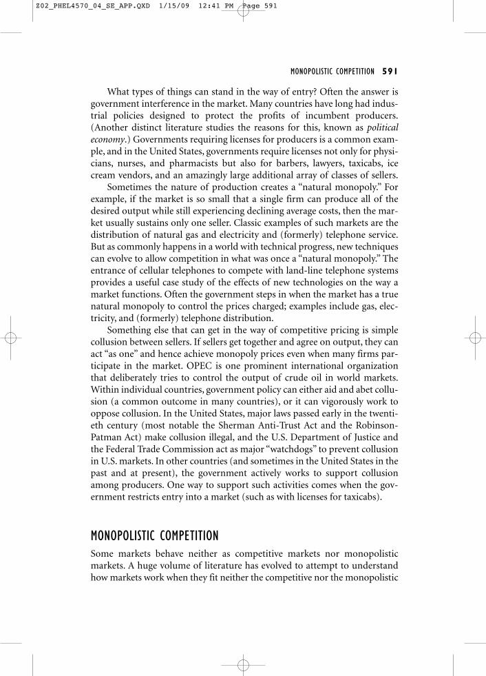
Figure A.8 shows the final equilibrium picture for each firm in the market.The demand curve still slopes downward (because incomplete shopping mixesin some of the slope of the market demand curve with the flat demand curveof pure competition). However, profits must fall to zero because of the pre-sumption of completely free (unfettered) entry. The latter condition occurswhen the average costs of production just match the price received by the firm.Thus, to understand the monopolistically competitive equilibrium, we need toknow the average cost curve of the firm (but not its marginal cost as in the caseof purely competitive markets or monopoly markets). Entry by competitorsspreads the available customers around to different firms, which we portray byshowing that as entry occurs, the demand curve for the firm shifts inward(while still retaining a nonzero slope because of incomplete shopping). The



p

X

AC

Dmc

pmc

pc

XcXmc

FIGURE A.8

shift inward can and must continue only to the point at which revenue fromsales just covers costs of production. This takes place when the demand curvefor each firm has shifted in to the point at which it just touches the AC curveof the firm at one point (on the left-hand branch of the AC curve). Thisdefines the monopolistically competitive equilibrium: Each firm’s demandcurve is tangent to its AC curve, so each firm makes no unusually large profits,and each firm faces a downward sloping demand curve.

The equilibrium price charged by this firm will be and its output willbe Obviously, the price will be higher than the competitive case [wherePc = min(AC)], and each firm’s output will be lower than would occur in acompetitive market. As a final observation, we might note that if the extent ofcomparison shopping increased sufficiently, the demand curves facing eachfirm would rotate more and more toward the flat demand curves facing acompetitive firm, and when enough shopping takes place (it turns out not torequire 100% of the buyers to carry out comparison shopping), the market“collapses” to the competitive equilibrium.

Xmc.pmc


introduction to basic economics...

Documents