introduction: sensors and rcs

AY2011v2 1

Introduction: Sensors and RCS (Chapter 1)

EC4630 Radar and Laser Cross Section

Fall AY2010 Prof. D. Jenn [email protected]

mailto:[email protected]

AY2011v2 2

Naval Postgraduate School Department of Electrical & Computer Engineering Monterey, California

Sensors and Signatures

• Sensors collect data • Sensor categories:

1. Active (has a transmitter) vs. passive (only listens) 2. Imaging (determines target features) vs. nonimaging (measures presence and

movement)

• Sensor performance measures and attributes

1. Detection range 2. Resolution 3. Field of view (FOV) 4. Data collection rate 5. Operating frequency band or regime: electromagnetic (IR, UV, MM, or radar),

visual (as it relates to human vision), or acoustic

• Related issues 1. Target signatures 2. Probability of intercept (“quietness” of a system, covertness) 3. Jamming and countermeasures to jamming 4. Data fusing (network centric approaches) 5. Background and clutter

AY2011v2 3


Sensor System Components

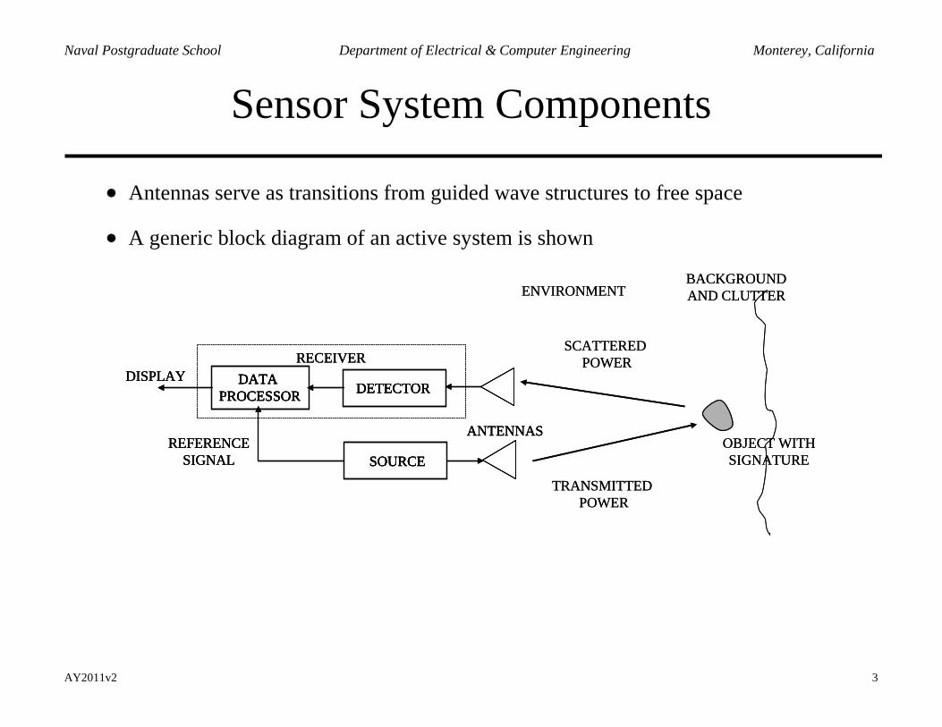
• Antennas serve as transitions from guided wave structures to free space

• A generic block diagram of an active system is shown

SCATTERED POWER

TRANSMITTED POWER

OBJECT WITHSIGNATURE

BACKGROUNDAND CLUTTERENVIRONMENT

DETECTORDATA PROCESSOR

ANTENNAS

DISPLAY

REFERENCESIGNAL SOURCE

RECEIVERSCATTERED

POWER

TRANSMITTED POWER

OBJECT WITHSIGNATURE

BACKGROUNDAND CLUTTERENVIRONMENT

DETECTORDATA PROCESSOR

ANTENNAS

DISPLAY

REFERENCESIGNAL SOURCE

RECEIVER

DETECTORDETECTORDATA PROCESSOR

DATA PROCESSOR

ANTENNAS

DISPLAY

REFERENCESIGNAL SOURCESOURCE

RECEIVER

AY2011v2 4


Non-imaging vs. Imaging Sensors

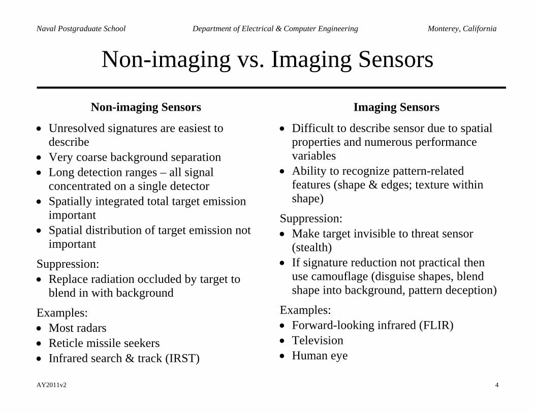
Non-imaging Sensors

• Unresolved signatures are easiest to describe

• Very coarse background separation • Long detection ranges – all signal

concentrated on a single detector • Spatially integrated total target emission

important • Spatial distribution of target emission not

important

Suppression: • Replace radiation occluded by target to

blend in with background

Examples: • Most radars • Reticle missile seekers • Infrared search & track (IRST)

Imaging Sensors

• Difficult to describe sensor due to spatial properties and numerous performance variables

• Ability to recognize pattern-related features (shape & edges; texture within shape)

Suppression: • Make target invisible to threat sensor

(stealth) • If signature reduction not practical then

use camouflage (disguise shapes, blend shape into background, pattern deception)

Examples: • Forward-looking infrared (FLIR) • Television • Human eye

AY2011v2 5


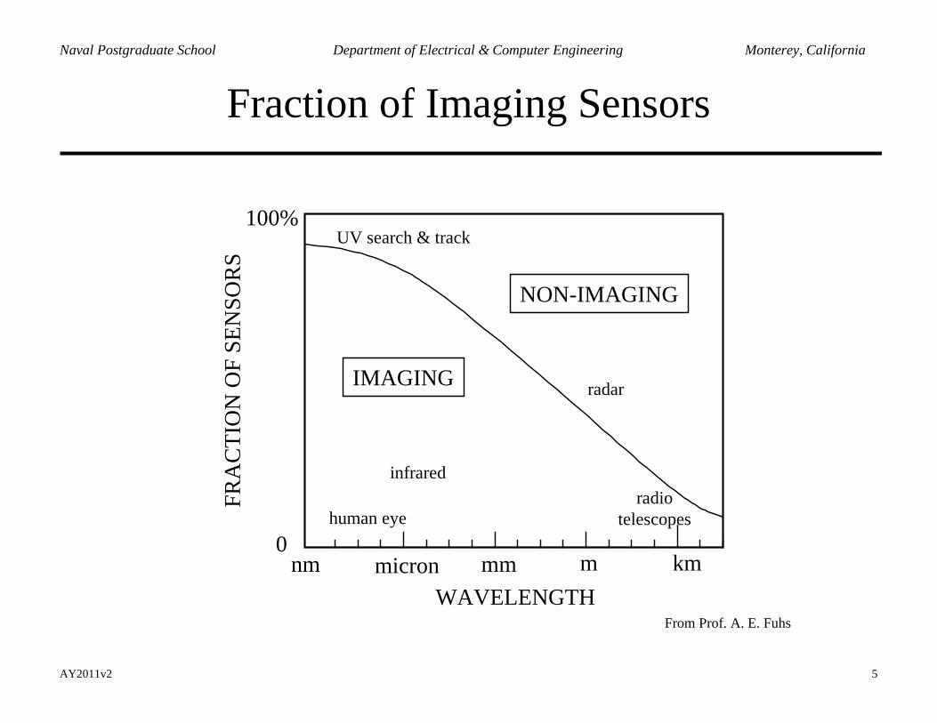
Fraction of Imaging Sensors

100%

0

FRA

CTI

ON

OF

SEN

SOR

S

WAVELENGTHnm mmmicron m km

infrared

human eye

UV search & track

NON-IMAGING

IMAGING

radiotelescopes

radar

From Prof. A. E. Fuhs

AY2011v2 6


Performance Tradeoffs for Sensors

Sensor Advantages Issues Forward looking Infrared (FLIR)

• High target to background contrast • Day or night operation • Penetrates fog, haze and dust

• False alarms from background clutter • Range uncertainty • Occlusions from terrain and vegetation • Aspect angle dependence

Millimeter wave (MMW) radar

• All weather operation • Day and night operation

• False alarms from background clutter, rocks, building, etc.

• Terrain occlusions • Signature varies with aspect angle

Synthetic aperture radar (SAR)

• All weather operation • Day and night operation • Large target to background contrast

• False alarms from background clutter, rocks, building, etc.

• Terrain occlusions • Signature varies with aspect angle

Laser radar • High range resolution • Doppler measurement • Imaging capability • Penetrates fog, haze and dust

• Signature varies with aspect angle • Complex system and technology • Requires long dwell time • Requires precise tracking and stabilization

Passive electro- optic (EO)

• Lightweight • Inexpensive • High resolution • Reliable

• Relatively low target to background contrast • No night or all weather capability

AY2011v2 7


Camouflage and Stealth

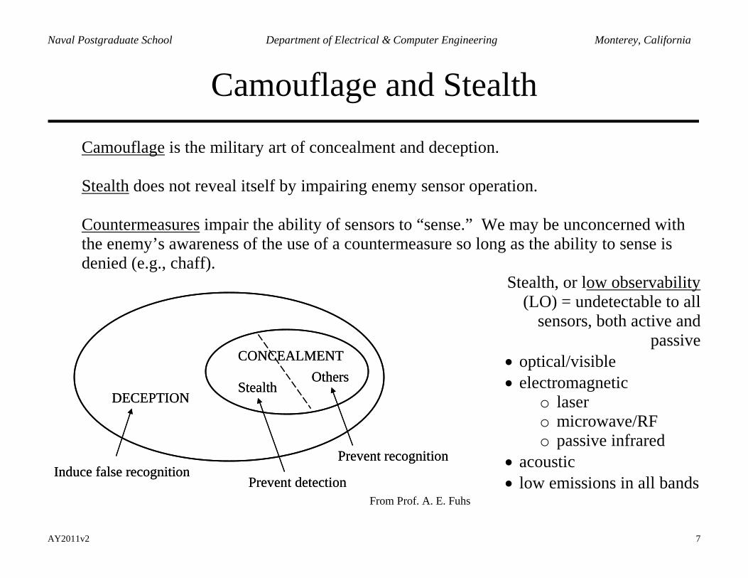
Camouflage is the military art of concealment and deception.

Stealth does not reveal itself by impairing enemy sensor operation.

Countermeasures impair the ability of sensors to “sense.” We may be unconcerned with the enemy’s awareness of the use of a countermeasure so long as the ability to sense is denied (e.g., chaff).

DECEPTIONStealth

OthersCONCEALMENT

Induce false recognitionPrevent detection

Prevent recognition

DECEPTIONStealth

OthersCONCEALMENT

Induce false recognitionPrevent detection

Prevent recognition

From Prof. A. E. Fuhs

Stealth, or low observability (LO) = undetectable to all

sensors, both active and passive

• optical/visible • electromagnetic

o laser o microwave/RF o passive infrared

• acoustic • low emissions in all bands

AY2011v2 8


Sensors and Low Observables (Stealth)

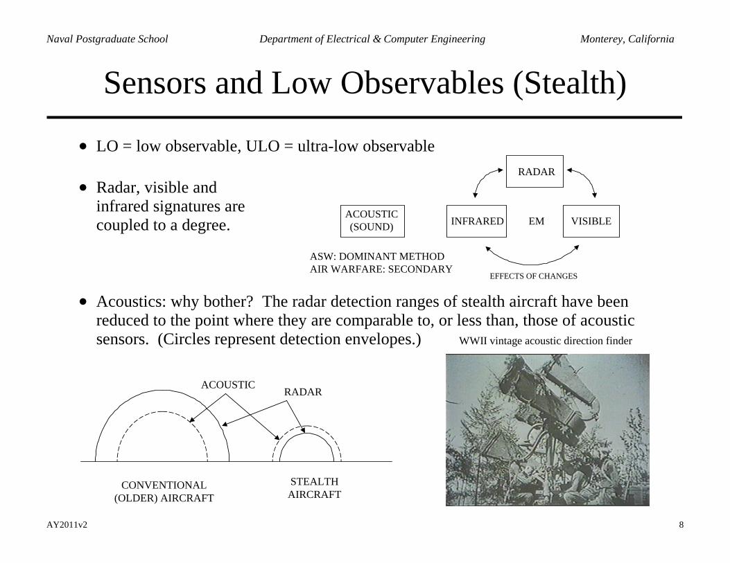
• LO = low observable, ULO = ultra-low observable

• Radar, visible and infrared signatures are coupled to a degree.

ACOUSTIC(SOUND)

RADAR

INFRARED VISIBLEEM

ASW: DOMINANT METHODAIR WARFARE: SECONDARY

EFFECTS OF CHANGES

• Acoustics: why bother? The radar detection ranges of stealth aircraft have been reduced to the point where they are comparable to, or less than, those of acoustic sensors. (Circles represent detection envelopes.) WWII vintage acoustic direction finder

ACOUSTICRADAR

CONVENTIONAL(OLDER) AIRCRAFT

STEALTHAIRCRAFT

AY2011v2 9


Bistatic vs. Monostatic Radar

TARGET

TRANSMITTER (TX)

RECEIVER (RX)

INCIDENT WAVE FRONTS

SCATTERED WAVE FRONTS

Rt

Rrβ TARGET

TRANSMITTER (TX)

RECEIVER (RX)

INCIDENT WAVE FRONTS

SCATTERED WAVE FRONTS

RtRt

RrRrβ

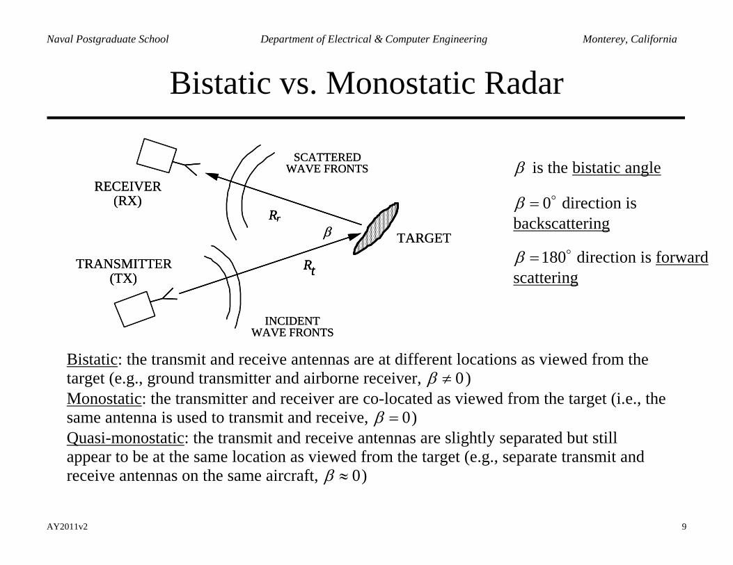
β is the bistatic angle

0β = direction is backscattering

180β = direction is forward scattering

Bistatic: the transmit and receive antennas are at different locations as viewed from the target (e.g., ground transmitter and airborne receiver, 0β ≠ ) Monostatic: the transmitter and receiver are co-located as viewed from the target (i.e., the same antenna is used to transmit and receive, 0β = ) Quasi-monostatic: the transmit and receive antennas are slightly separated but still appear to be at the same location as viewed from the target (e.g., separate transmit and receive antennas on the same aircraft, 0β ≈ )

AY2011v2 10


Basic Radar Range Equation (1)

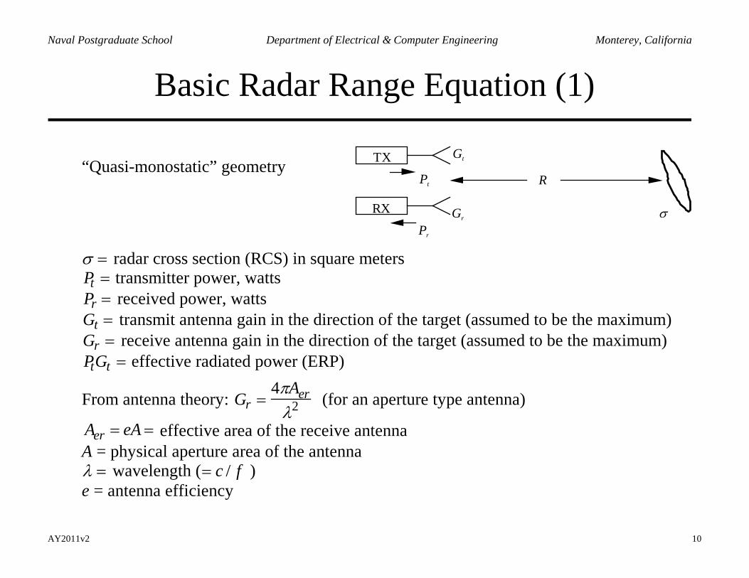
“Quasi-monostatic” geometry

R

TX

Pt

Gt

RX

Pr

Gr σ

σ = radar cross section (RCS) in square meters Pt = transmitter power, watts Pr = received power, watts Gt = transmit antenna gain in the direction of the target (assumed to be the maximum) Gr = receive antenna gain in the direction of the target (assumed to be the maximum) PtGt = effective radiated power (ERP)

From antenna theory: Gr =4πAer

λ2 (for an aperture type antenna)

erA eA= = effective area of the receive antenna A = physical aperture area of the antenna λ = wavelength (= c / f ) e = antenna efficiency

AY2011v2 11



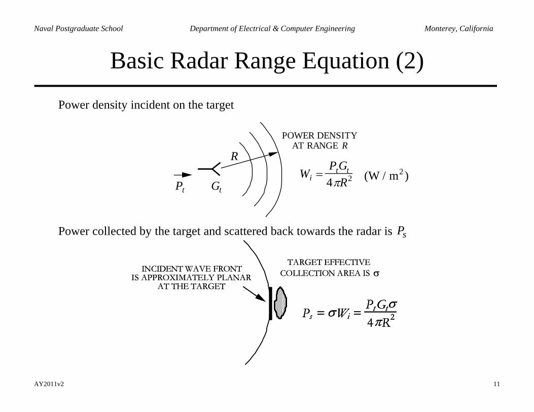
Power density incident on the target

Pt Gt

RWi =

PtGt

4πR2

POWER DENSITY AT RANGE R

(W / m2 )

Power collected by the target and scattered back towards the radar is sP

INCIDENT WAVE FRONT IS APPROXIMATELY PLANAR

AT THE TARGET

TARGET EFFECTIVE COLLECTION AREA IS σ

Ps = σWi = Pt Gtσ4πR2

INCIDENT WAVE FRONT IS APPROXIMATELY PLANAR

AT THE TARGET

TARGET EFFECTIVE COLLECTION AREA IS σ

Ps = σWi = Pt Gtσ4πR2Ps = σWi = Pt Gtσ4πR2

AY2011v2 12



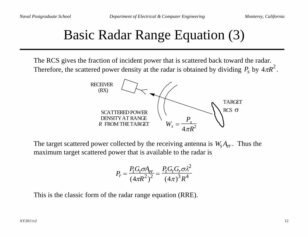
The RCS gives the fraction of incident power that is scattered back toward the radar. Therefore, the scattered power density at the radar is obtained by dividing sP by 4πR2 .

TARGET RCS σ

RECEIVER (RX)

Ws =Ps

4πR2

SCATTERED POWER DENSITY AT RANGE

R FROM THE TARGET

The target scattered power collected by the receiving antenna is Ws Aer . Thus the maximum target scattered power that is available to the radar is

Pr =PtGtσAer(4πR2 )2 =

PtGtGrσλ2

(4π )3 R4

This is the classic form of the radar range equation (RRE).

AY2011v2 13


Characteristics of the Radar Range Equation

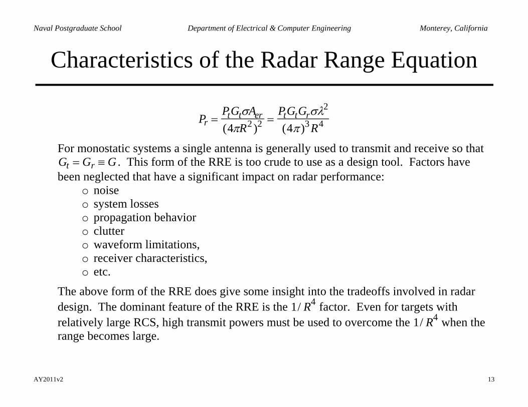
Pr =PtGtσAer(4πR2 )2 =

PtGtGrσλ2

(4π )3R4

For monostatic systems a single antenna is generally used to transmit and receive so that Gt = Gr ≡ G . This form of the RRE is too crude to use as a design tool. Factors have been neglected that have a significant impact on radar performance:

o noise o system losses o propagation behavior o clutter o waveform limitations, o receiver characteristics, o etc.

The above form of the RRE does give some insight into the tradeoffs involved in radar design. The dominant feature of the RRE is the 1/ R4 factor. Even for targets with relatively large RCS, high transmit powers must be used to overcome the 1/ R4 when the range becomes large.

AY2011v2 14


Maximum Detection Range

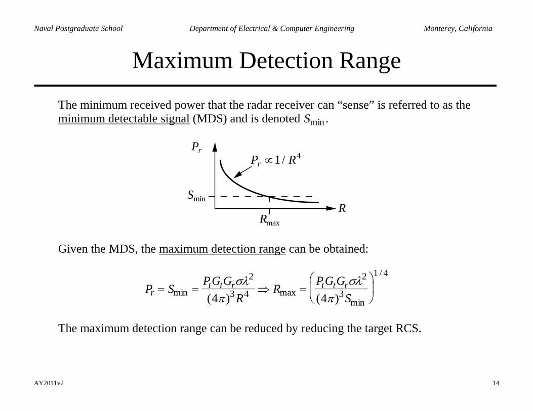
The minimum received power that the radar receiver can “sense” is referred to as the minimum detectable signal (MDS) and is denoted Smin .

SminR

PrPr ∝1/ R4

Rmax

Given the MDS, the maximum detection range can be obtained:

Pr = Smin =PtGtGrσλ2

(4π )3R4 ⇒ Rmax =PtGtGrσλ2

(4π )3Smin

1 / 4

The maximum detection range can be reduced by reducing the target RCS.

AY2011v2 15


Other Radar System Factors

Radars typically operate in a “noise limited” condition. The target’s received power must be greater than the receiver noise power. The noise power is generally modeled as Gaussian white noise

TBo sN k B= The signal-to-noise ratio (SNR) is

TB

r pro s

P G LPSNRN k B

= =

where: 231.38 10Bk −= × = Boltzman’s constant (J/K) B = bandwidth (Hz)

T T Ts A e= + = system noise temperature (K) TA = antenna temperature (K) Te =effective noise temperature of the receiver (K)

pG = processing gain (resulting from integration, correlation, or signal processing, etc.) L = loss factor ( )1≤ for system hardware and processing losses

Typically SNRs of 10 to 20 dB are required for acceptable detection and tracking.

AY2011v2 16


Search Radar Example (1)

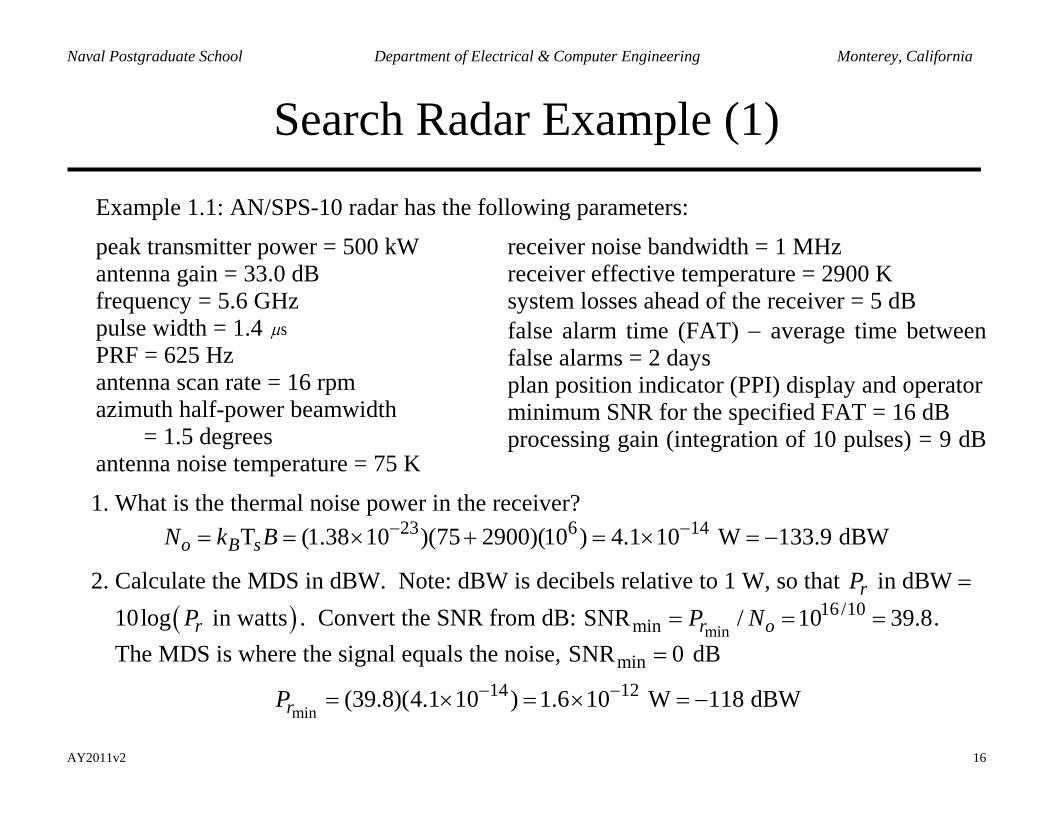
Example 1.1: AN/SPS-10 radar has the following parameters:

peak transmitter power = 500 kW antenna gain = 33.0 dB frequency = 5.6 GHz pulse width = 1.4 µs PRF = 625 Hz antenna scan rate = 16 rpm azimuth half-power beamwidth

= 1.5 degrees antenna noise temperature = 75 K

receiver noise bandwidth = 1 MHz receiver effective temperature = 2900 K system losses ahead of the receiver = 5 dB false alarm time (FAT) − average time between false alarms = 2 days plan position indicator (PPI) display and operator minimum SNR for the specified FAT = 16 dB processing gain (integration of 10 pulses) = 9 dB

1. What is the thermal noise power in the receiver? 23 6 14T (1.38 10 )(75 2900)(10 ) 4.1 10 W 133.9 dBWo B sN k B − −= = × + = × = −

2. Calculate the MDS in dBW. Note: dBW is decibels relative to 1 W, so that in dBWrP = ( )10log in wattsrP . Convert the SNR from dB:

min16 /10

minSNR / 10 39.8r oP N= = = . The MDS is where the signal equals the noise, minSNR 0= dB

min14 12(39.8)(4.1 10 ) 1.6 10 W 118 dBWrP − −= × = × = −

AY2011v2 17


Search Radar Example (2)

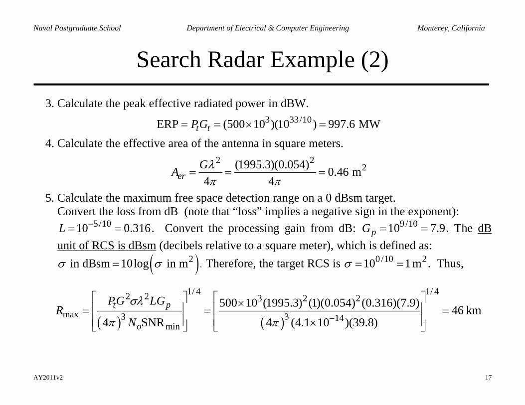
3. Calculate the peak effective radiated power in dBW.

3 33/10ERP (500 10 )(10 ) 997.6 MWt tPG= = × = 4. Calculate the effective area of the antenna in square meters.

2 22(1995.3)(0.054) 0.46 m

4 4erGA λ

π π= = =

5. Calculate the maximum free space detection range on a 0 dBsm target. Convert the loss from dB (note that “loss” implies a negative sign in the exponent):

5/1010 0.316L −= = . Convert the processing gain from dB: 9 /1010 7.9pG = = . The dB unit of RCS is dBsm (decibels relative to a square meter), which is defined as:

( )2 in dBsm 10log in mσ σ= . Therefore, the target RCS is 0 /10 210 1 mσ = = . Thus,

( ) ( )

1/ 4 1/ 42 2 3 2 2

max 3 3 14min

500 10 (1995.3) (1)(0.054) (0.316)(7.9) 46 km4 SNR 4 (4.1 10 )(39.8)

t p

o

PG LGR

N

σλ

π π −

× = = = ×

AY2011v2 18


Antenna as a Radar Target

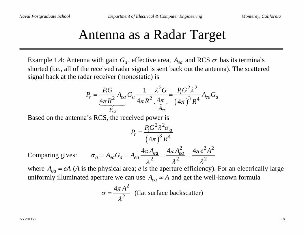
Example 1.4: Antenna with gain aG , effective area, eaA and RCS σ has its terminals shorted (i.e., all of the received radar signal is sent back out the antenna). The scattered signal back at the radar receiver (monostatic) is

( )

2 22

2 2 3 41

44 4 4erra

t tr ea a ea a

AP

PG PGGP A G A GR R R

λλππ π π

=

= =

Based on the antenna’s RCS, the received power is

( )

2 2

3 44t a

rPGP

R

λ σ

π=

Comparing gives: 2 2 2

2 2 24 4 4ea ea

a ea a eaA A e AA G A π π πσ

λ λ λ= = = =

where eaA eA= (A is the physical area; e is the aperture efficiency). For an electrically large uniformly illuminated aperture we can use eaA A≈ and get the well-known formula

2

24 Aπσ

λ= (flat surface backscatter)

AY2011v2 19


Flat Surface Backscatter Formula

The “flat surface backscatter formula” applies to any arbitrary contoured flat surface of area

A. Normal incidence on a plane surface gives 2

22

4 mAπσλ

= . The decibel unit is decibels

relative to a square meter (dBsm) defined as: 210, dBsm 10log ( , m )σ σ=

Example 1.5: Normal incidence on a L by L square plate with L = 1 m

At 300 MHz, 1λ = m: 22

22

4 (1)=12.56 m 11 dBsm

1

πσ

= =

At 3 GHz, 0.1λ = m: 22

22

4 (1)=1256 m 31 dBsm

0.1

πσ

= =

Note the “gain” effect with increasing frequency (similar to an aperture antenna). A 1 2m

area plate has a much higher RCS than 1 2m at these frequencies. This is because the plate scattering has some directivity (i.e., it does not scatter isotropically).

AY2011v2 20


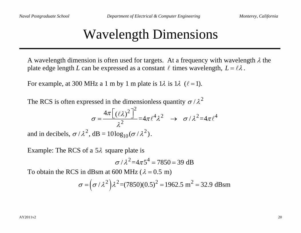
Wavelength Dimensions

A wavelength dimension is often used for targets. At a frequency with wavelength λ the plate edge length L can be expressed as a constant times wavelength, L λ= . For example, at 300 MHz a 1 m by 1 m plate is 1λ is 1λ ( 1).= The RCS is often expressed in the dimensionless quantity 2/σ λ

224 2 2 4

2

4 ( )=4 / =4

π λσ π λ σ λ π

λ

= →

and in decibels, 2 210/ , dB = 10log ( / )σ λ σ λ .

Example: The RCS of a 5λ square plate is

2 4/ =4 5 7850 39 dBσ λ π = = To obtain the RCS in dBsm at 600 MHz ( 0.5λ = m)

( )2 2 2 2/ =(7850)(0.5) 1962.5 m 32.9 dBsmσ σ λ λ= = =

AY2011v2 21


Scattering Nomenclature

INDUCEDCURRENTS TARGET

INCIDENTPLANE WAVE

SCATTEREDSPHERICAL

WAVE

INDUCEDCURRENTS TARGETTARGET

INCIDENTPLANE WAVE

SCATTEREDSPHERICAL

WAVER

INDUCEDCURRENTS TARGET

INCIDENTPLANE WAVE

SCATTEREDSPHERICAL

WAVE

INDUCEDCURRENTS TARGETTARGET

INCIDENTPLANE WAVE

SCATTEREDSPHERICAL

WAVER

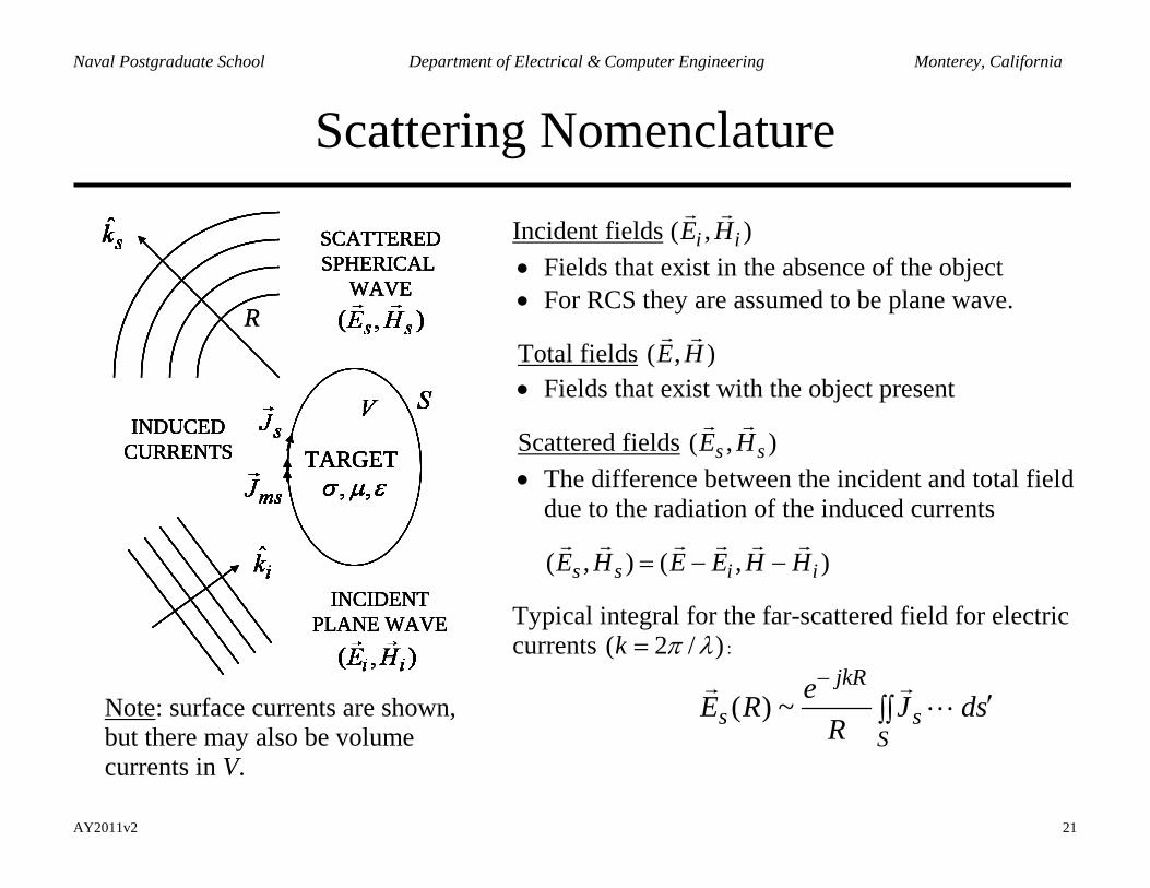
Note: surface currents are shown, but there may also be volume currents in V.

Incident fields ( , )i iE H

• Fields that exist in the absence of the object • For RCS they are assumed to be plane wave.

Total fields ( , )E H

• Fields that exist with the object present

Scattered fields ( , )s sE H

• The difference between the incident and total field

due to the radiation of the induced currents

( , ) ( , )s s i iE H E E H H= − −

Typical integral for the far-scattered field for electric currents ( 2 / )k π λ= :

( ) ~jkR

s sS

eE R J dsR

−′∫∫

AY2011v2 22


Definition of RCS

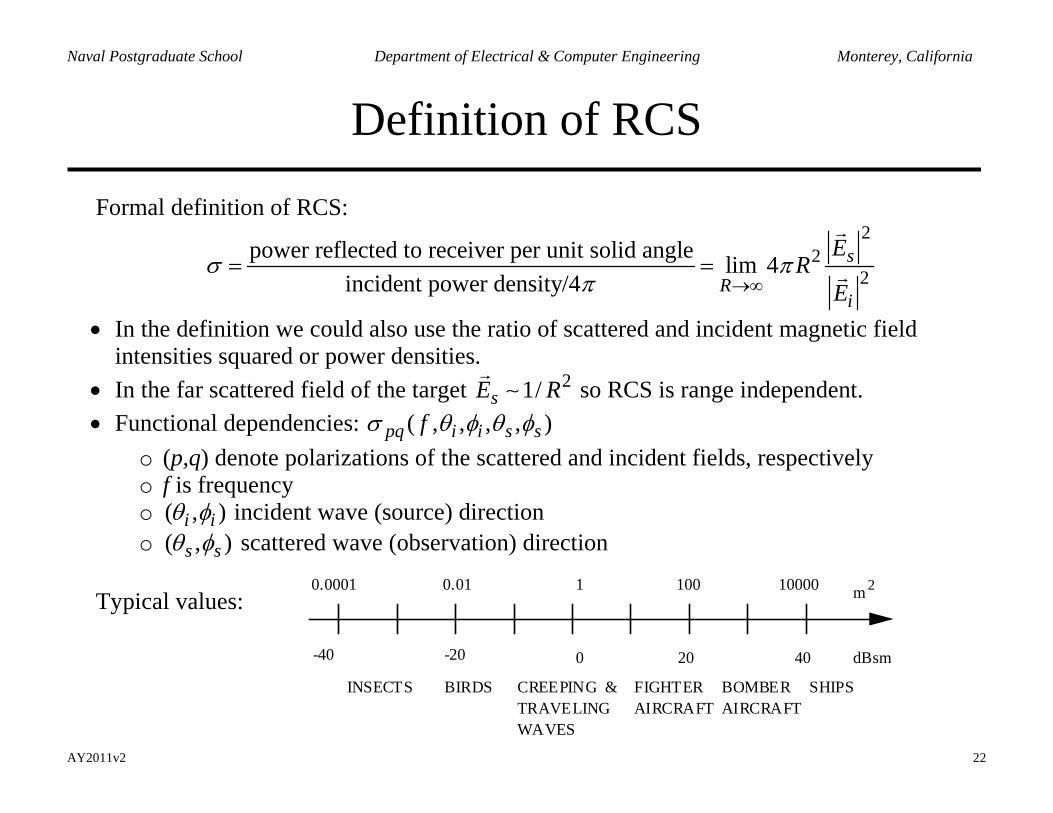
Formal definition of RCS:

22

2power reflected to receiver per unit solid angle lim 4

incident power density/4s

Ri

ER

Eσ π

π →∞= =

• In the definition we could also use the ratio of scattered and incident magnetic field intensities squared or power densities.

• In the far scattered field of the target 21/sE R

so RCS is range independent. • Functional dependencies: ( , , , , )pq i i s sfσ θ φ θ φ

o (p,q) denote polarizations of the scattered and incident fields, respectively o f is frequency o ( , )i iθ φ incident wave (source) direction o ( , )s sθ φ scattered wave (observation) direction

Typical values:

-40 -20 0 20 40 dBsm

m 20.0001 0.01 1 100 10000

INSECTS BIRDS CREEPING & TRAVELING WAVES

FIGHTER AIRCRAFT

BOMBER AIRCRAFT

SHIPS

AY2011v2 23


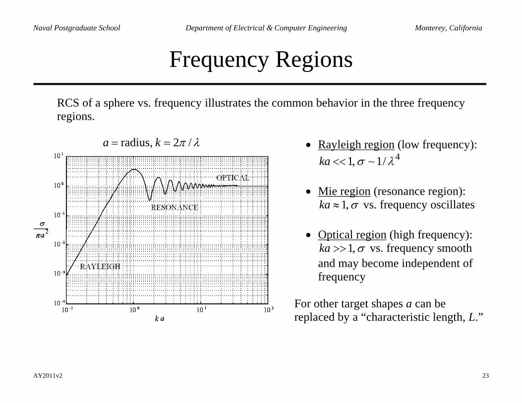
Frequency Regions

RCS of a sphere vs. frequency illustrates the common behavior in the three frequency regions.

radius, 2 /a k π λ= =

• Rayleigh region (low frequency):

41, 1/ka σ λ<<

• Mie region (resonance region): 1,ka σ≈ vs. frequency oscillates

• Optical region (high frequency):

1,ka σ>> vs. frequency smooth and may become independent of frequency

For other target shapes a can be replaced by a “characteristic length, L.”

AY2011v2 24


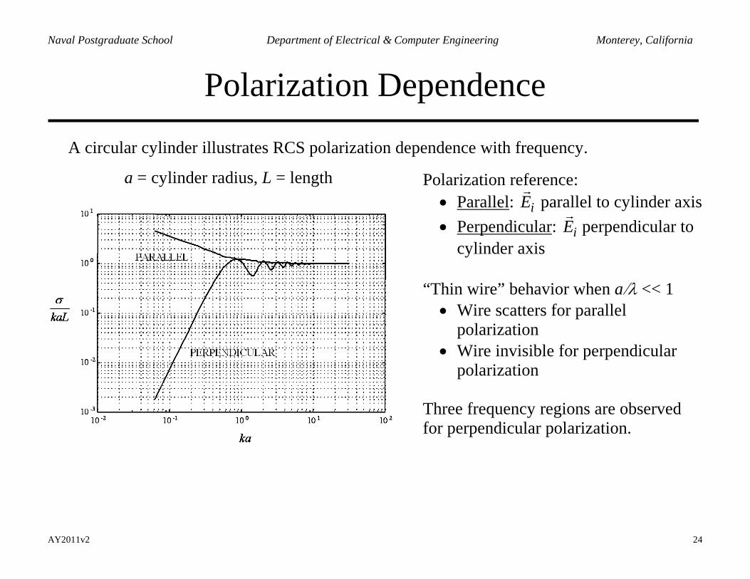
Polarization Dependence

A circular cylinder illustrates RCS polarization dependence with frequency.

a = cylinder radius, L = length

Polarization reference:

• Parallel: iE

parallel to cylinder axis • Perpendicular: iE

perpendicular to cylinder axis

“Thin wire” behavior when a/λ << 1

• Wire scatters for parallel polarization

• Wire invisible for perpendicular polarization

Three frequency regions are observed for perpendicular polarization.

AY2011v2 25


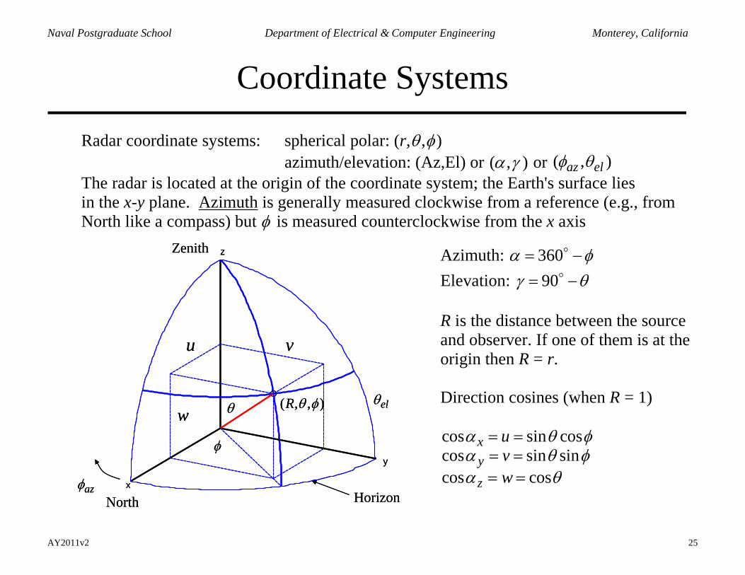
Coordinate Systems

Radar coordinate systems: spherical polar: (r,θ ,φ) azimuth/elevation: (Az,El) or (α ,γ ) or ( , )az elφ θ The radar is located at the origin of the coordinate system; the Earth's surface lies

in the x-y plane. Azimuth is generally measured clockwise from a reference (e.g., from North like a compass) but φ is measured counterclockwise from the x axis

y

z

x

θ elθ

azφ

φ

( , , )R θ φ

u v

w

Zenith

North Horizon

y

z

x

θ elθ

azφ

φ

( , , )R θ φ

u v

w

Zenith

North Horizon

Azimuth: 360α φ= − Elevation: 90γ θ= − R is the distance between the source and observer. If one of them is at the origin then R = r. Direction cosines (when R = 1) cos sin coscos sin sincos cos

xy

z

uvw

α θ φα θ φα θ

= == == =

AY2011v2 26


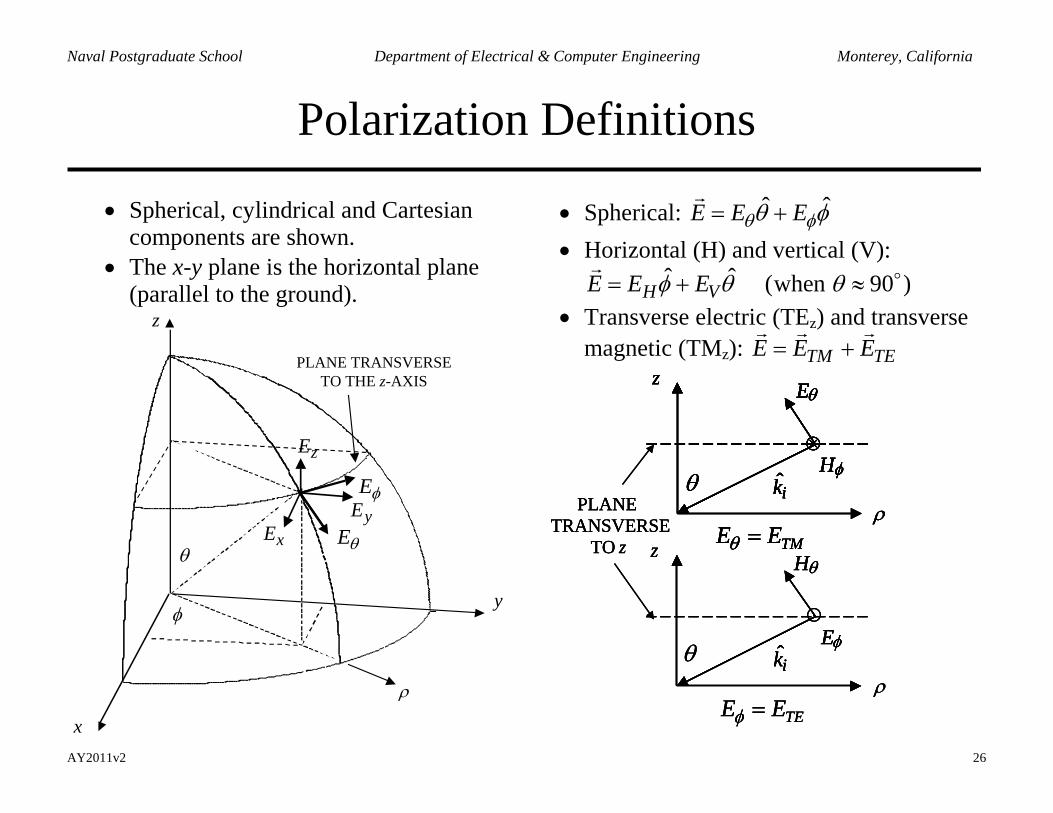
Polarization Definitions

• Spherical, cylindrical and Cartesian components are shown.

• The x-y plane is the horizontal plane (parallel to the ground).

φ

θ

z

x

y

θE

φE

PLANE TRANSVERSETO THE z-AXIS

ρ

xE

zE

yE

• Spherical: ˆ ˆE E Eθ φθ φ= +

• Horizontal (H) and vertical (V):

ˆ ˆ (when 90 )H VE E Eφ θ θ= + ≈

• Transverse electric (TEz) and transverse

magnetic (TMz): TM TEE E E= +

PLANE TRANSVERSE

TO z TME Eθ =

θE

ρ

z

ikHφ

⊗

θ

Hθ

ρ

z

ikEφ

θ

TEE Eφ =

PLANE TRANSVERSE

TO z

PLANE TRANSVERSE

TO z TME Eθ =

θE

ρ

z

ikHφ

⊗

θ

Hθ

ρ

z

ikEφ

θ

TEE Eφ =

TME Eθ =

θE

ρ

z

ikHφ

⊗

θ

TME Eθ =

θE

ρ

z

ikHφ

⊗

θEθE

ρ

z

ikikHφHφ

⊗

θ

HθHθ

ρ

z

ikikEφEφ

θ

TEE Eφ =

AY2011v2 27


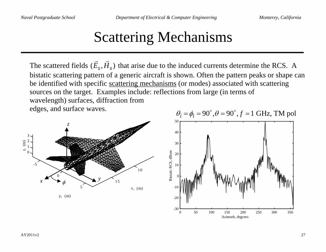
Scattering Mechanisms

The scattered fields ( , )s sE H

that arise due to the induced currents determine the RCS. A bistatic scattering pattern of a generic aircraft is shown. Often the pattern peaks or shape can be identified with specific scattering mechanisms (or modes) associated with scattering sources on the target. Examples include: reflections from large (in terms of wavelength) surfaces, diffraction from edges, and surface waves.

10

15

-5

0

5

0123

x, (m)

y, (m)

z, (

m)

φx y

z

90 , 90 , 1 GHz, TM poli i fθ φ θ= = = =

0 50 100 150 200 250 300 350-30

-20

-10

0

10

20

30

40

50

Azimuth, degrees

Bist

atic

RCS

, dB

sm

AY2011v2 28


Illustration of Scattering Mechanisms

SPECULAR

DUCTING, WAVEGUIDE MODES

MULTIPLE REFLECTIONS

EDGE DIFFRACTION

SURFACE WAVES

CREEPING WAVES

Important scattering mechanisms: • Reflections, multiple

reflections (multipath) • Diffraction from edges • Surface waves

o Travelling waves o Creeping waves o Leaky waves

• Ducting (waveguide or cavity modes)

• Hybrid or “mixed” modes

Reduction techniques are dependent on the scattering source and mechanism.

AY2011v2 29


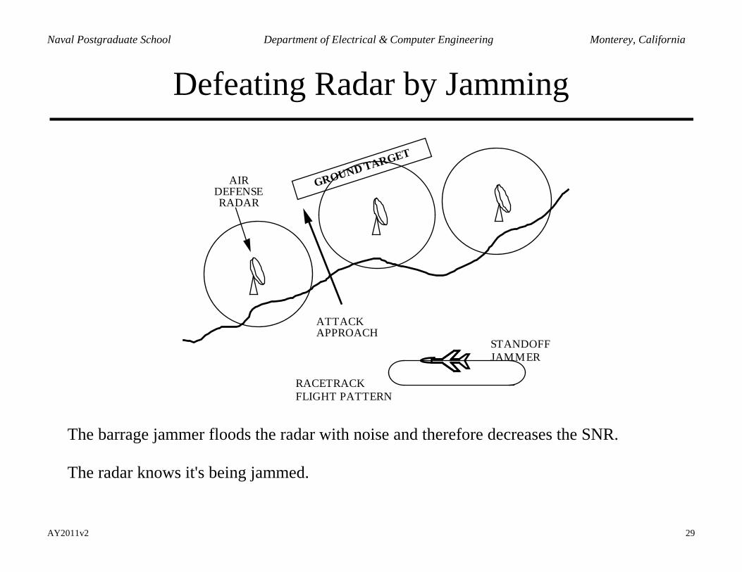
Defeating Radar by Jamming

GROUND TARGET

AIR DEFENSE RADAR

ATTACK APPROACH

STANDOFF JAMMER

RACETRACK FLIGHT PATTERN

The barrage jammer floods the radar with noise and therefore decreases the SNR. The radar knows it's being jammed.

AY2011v2 30


Jammer Burnthrough Range (1)

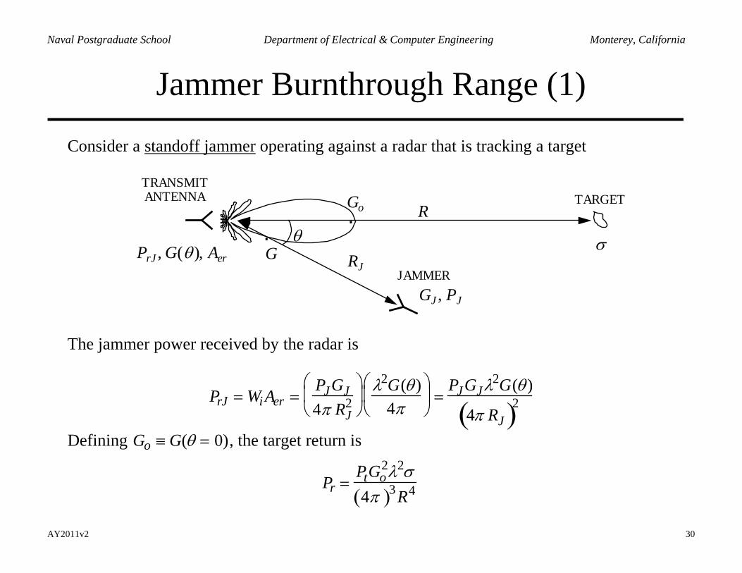
Consider a standoff jammer operating against a radar that is tracking a target

R

RJ

Go

G

.. σ

TRANSMIT ANTENNA TARGET

JAMMERGJ , PJ

θPrJ , G(θ), Aer

The jammer power received by the radar is

PrJ = Wi Aer =PJGJ4π RJ

2

λ2G(θ)

4π

=

PJGJλ2G(θ)

4π RJ( )2

Defining Go ≡ G(θ = 0), the target return is

Pr =PtGo

2λ2σ4π( )3R4

AY2011v2 31


Jammer Burnthrough Range (2)

The signal-to-jam ratio is

SJR =SJ

=PrPrJ

=PtGoPJGJ

RJ

2

R4

σ

4π

GoG(θ )

The burnthrough range for the jammer is the range at which its signal is equal to the target return (SJR=1).

Important points:

o RJ2 vs R4 is a big advantage for the jammer.

o G vs G(θ ) is usually a big disadvantage for the jammer. Low sidelobe radar antennas reduce jammer effectiveness.

o Given the geometry, the only parameter that the jammer has control of is the ERP (PJGJ ).

o The radar knows it is being jammed. The jammer can be countered using waveform selection and signal processing techniques.

AY2011v2 32


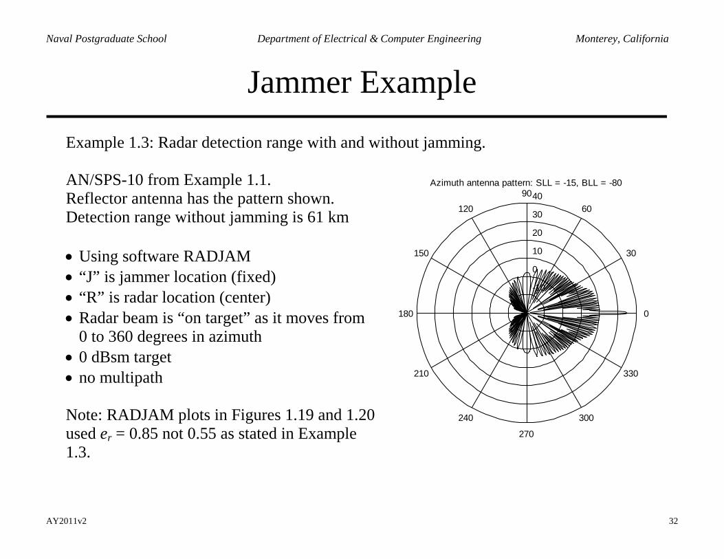
Jammer Example

Example 1.3: Radar detection range with and without jamming. AN/SPS-10 from Example 1.1. Reflector antenna has the pattern shown. Detection range without jamming is 61 km • Using software RADJAM • “J” is jammer location (fixed) • “R” is radar location (center) • Radar beam is “on target” as it moves from

0 to 360 degrees in azimuth • 0 dBsm target • no multipath Note: RADJAM plots in Figures 1.19 and 1.20 used er = 0.85 not 0.55 as stated in Example 1.3.

-10

0

10

20

30

40

30

210

60

240

90

270

120

300

150

330

180 0

Azimuth antenna pattern: SLL = -15, BLL = -80

AY2011v2 33


Jammer Example

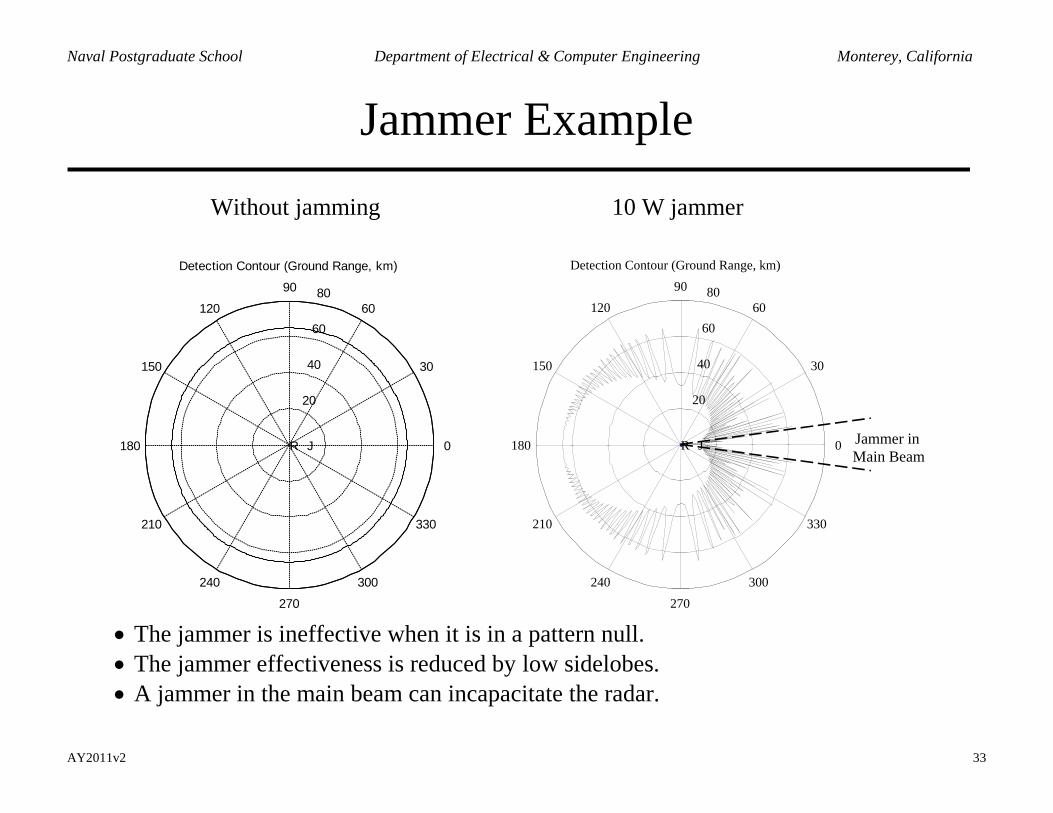
Without jamming 10 W jammer

20

40

60

80

30

210

60

240

90

270

120

300

150

330

180 0

Detection Contour (Ground Range, km)

R J

20

40

60

80

30

210

60

240

90

270

120

300

150

330

180 0

Detection Contour (Ground Range, km)

R J Jammer inMain Beam

• The jammer is ineffective when it is in a pattern null. • The jammer effectiveness is reduced by low sidelobes. • A jammer in the main beam can incapacitate the radar.

AY2011v2 34


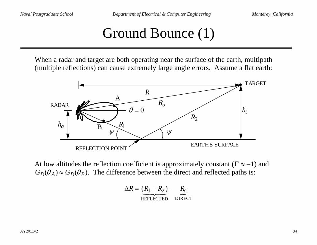
Ground Bounce (1)

When a radar and target are both operating near the surface of the earth, multipath (multiple reflections) can cause extremely large angle errors. Assume a flat earth:

.

EARTH'S SURFACE

Ro

R1R2

RADAR

TARGET•

ha

ht•

A

B

R

ψψ

θ = 0

REFLECTION POINT

At low altitudes the reflection coefficient is approximately constant (Γ ≈ −1) and GD(θ A) ≈ GD(θB). The difference between the direct and reflected paths is:

∆R = (R1 + R2 )REFLECTED

− RoDIRECT

AY2011v2 35


Ground Bounce (2)

The total signal at the target is:

Etot = ErefREFLECTED

+ EdirDIRECT

= E(θA ) + Γ E(θB)e− jk∆R

From the low altitude approximation, Edir = E(θA) ≈ E(θB ) so that

Etot ≈ Edir + Γ Edire− jk∆R = Edir | 1+ Γ e− jk∆R[ ]

≡F, PATH GAINFACTOR

|

The path gain factor takes on the values 0 ≤ F ≤ 2. If F = 0 the direct and reflected rays cancel (destructive interference); if F = 2 the two waves add (constructive interference). An approximate expression for the path difference can be obtained as follows:

Ro = R2 + (ht − ha )2 ≈ R + 12

(ht − ha )2

R

R1 + R2 = R2 + (ht + ha )2 ≈ R + 12

(ht + ha )2

R

AY2011v2 36


Ground Bounce (3)

Therefore, ∆R ≈

2hahtR

and | F |= 1− e− jk2haht / R = e jkhaht / R e− jkhaht / R − e jkhaht / R( )= 2sin khaht / R( )

Incorporate the path gain factor into the RRE:

Pr ∝| F |4= 16sin 4 khthaR

≈ 16

kht haR

4

The last form is based on the small angle approximation

0t akh hR

→ .

Finally, the RRE can be written as

Pr =PtGtGrλ2σ(4π )3 R4 | F |4≈

4π PtGtGrσ (htha )4

λ2R8

AY2011v2 37


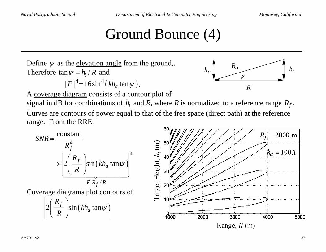
Ground Bounce (4)

Define ψ as the elevation angle from the ground,. Therefore tan /th Rψ = and

( )4 4| | 16sin tanaF kh ψ= . A coverage diagram consists of a contour plot of

R

Roψ

htha

signal in dB for combinations of th and R, where R is normalized to a reference range Rf . Curves are contours of power equal to that of the free space (direct path) at the reference range. From the RRE:

( )

4

4

/

constant

2 sin tan

f

f

fa

F R R

SNRR

Rkh

Rψ

=

×

Coverage diagrams plot contours of

( )2 sin tanfa

Rkh

Rψ

AY2011v2 38


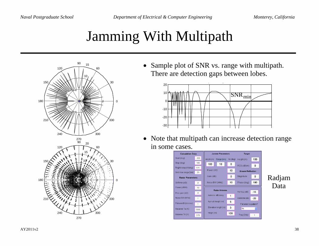
Jamming With Multipath

5

10

15

20

30

210

60

240

90

270

120

300

150

330

180 0

R J

5

10

15

30

210

60

240

90

270

120

300

150

330

180 0

R J

5

10

15

20

30

210

60

240

90

270

120

300

150

330

180 0

R J

5

10

15

30

210

60

240

90

270

120

300

150

330

180 0

R J

• Sample plot of SNR vs. range with multipath. There are detection gaps between lobes.

-30

-20

-10

0

10

20y g

minSNR

-30

-20

-10

0

10

20y g

minSNR

• Note that multipath can increase detection range in some cases.

RadjamData

introduction: sensors and rcs

Documents