introduction - sas

4 Generalized Linear and Nonlinear Models for Correlated Data

• Image analysisImage segmentation studies where the goal is to extract information about a particularregion of interest from a given image. For example, in the field of medicine, imagesegmentation may be required to identify tissue regions that have been stained versusnot stained. In these settings, modeling spatial correlation associated with a latticearray of pixel locations can help improve digital image analysis.

1.1.4 Multivariate data

Historically, the concept of correlation has been closely linked with methods for analyzingmultivariate data wherein two or more response variables are measured per experimentalunit or individual. Such methods include multivariate analysis of variance, cluster analysis,discriminant analysis, principal components analysis, canonical correlation analysis, etc.This book does not cover those topics but instead considers applications requiring theanalysis of multivariate repeated measurements or the joint modeling of repeatedmeasurements and one or more outcome measures that are measured only once. Exampleswe consider include

• Multivariate repeated measurementsAny study where one has two or more outcome variables measured repeatedly over time.

• Joint modeling of repeated measurements and event-times dataStudies where the primary goal is to draw inference on serial trends associated with aset of repeated measurements while accounting for possible informative censoring due todropout.Studies where the primary goal is to draw joint inference on patient outcomes (e.g.,patient survival) and any serial trends one might observe in a potential surrogatemarker of patient outcome.

Of course one can easily imagine applications that involve two or more types ofcorrelated data. For example, a longitudinal study may well entail both repeatedmeasurements taken at the individual level and clustered data where groups of individualsform clusters according to some pre-determined criteria (e.g., a group randomized trial).Spatio-temporal data such as found in the mapping of disease rates over time is anotherexample of combining two types of correlated data, namely spatially correlated data withserially correlated longitudinal data.

The majority of applications in this book deal with the analysis of repeatedmeasurements, longitudinal data, clustered data, and to a lesser extent, spatial data. Amore thorough treatment and illustration of applications involving the analysis of spatiallycorrelated data and panel data, for example, may found in other texts including Cressie(1993), Littell et. al. (2006), Hsiao (2003), Frees (2004) and Matyas and Sevestre (2008).We will also examine applications that require modeling multivariate repeatedmeasurements in which two or more response variables are measured on the sameexperimental unit or individual on multiple occasions. As the focus of this book is onapplications requiring the use of generalized linear and nonlinear models, examples willinclude methods for analyzing continuous, discrete and ordinal data including logisticregression for binary data, Poisson regression for counts, and nonlinear regression fornormally distributed data.

1.2 Explanatory variablesWhen analyzing correlated data, one need first consider the kind of study from which thedata were obtained. In this book, we consider data arising from two types of studies: 1)experimental studies, and 2) observational studies. Experimental studies are generally

Vonesh, Edward F. Generalized Linear and Nonlinear Models for Correlated Data: Theory and Applications Using SAS. Copyright © 2012, SAS Institute Inc., Cary, North Carolina, USA. ALL RIGHTS RESERVED. For additional SAS resources, visit support.sas.com/bookstore.

Chapter 1 Introduction 5

interventional in nature in that two or more treatments are applied to experimental unitswith a goal of comparing the mean response across different treatments. Such studies mayor may not entail randomization. For example, in a parallel group randomizedplacebo-controlled clinical trial, the experimental study may entail randomizing individualsinto two groups; those who receive the placebo control versus those who receive an activeingredient. In contrast, in a simple pre-post study, a measured response is obtained on allindividuals prior to receiving a planned intervention and then, following the intervention, asecond response is measured. In this case, although no randomization is performed, thestudy is still experimental in that it does entail a planned intervention. Whetherrandomization is performed or not, additional explanatory variables are usually collected soas to 1) adjust for any residual confounding that may be present with or withoutrandomization and 2) determine if interactions exist with the intervention.

In contrast to an experimental study, an observational study entails collecting data onavailable individuals from some target population. Such data would include any outcomemeasures of interest as well as any explanatory variables thought to be associated with theoutcome measures.

In both kinds of studies, the set of explanatory variables, or covariates, used to modelthe mean response can be broadly classified into two categories:

• Within-unit factors or covariates (in longitudinal studies, these are often referred to astime-dependent covariates or repeated measures factors).For repeated measurements and longitudinal studies, examples include time itself,different dose levels applied to the same individual in a dose-response study, differenttreatment levels given to the same individual in a crossover study.For clustered data, examples include any covariates measured on individuals within acluster.

• Between-unit factors or covariates (in longitudinal studies, these are often referred to astime-independent covariates)Examples include baseline characteristics in a longitudinal study (e.g., gender, race,baseline age), different treatment levels in a randomized prospective longitudinal study,different cluster-specific characteristics, etc.

It is important to maintain the distinction between these two types of covariates forseveral reasons. One, it helps remind us that within-unit covariates model unit-specifictrends while between-unit covariates model trends across units. Two, it may help informulating an appropriate variance-covariance structure depending on the degree ofheterogeneity between select groups of individuals or units. Finally, such distinctions areneeded when designing a study. For example, sample size will be determined, in large part,on the primary goals of a study. When those goals focus on comparisons that involvewithin-unit covariates (either main effects or interactions), the number of experimentalunits needed will generally be less than when based on comparisons involving strictlybetween-unit comparisons.

1.3 Types of modelsWhile there are several approaches to modeling correlated response data, we will confineourselves to two basic approaches, namely the use of 1) marginal models and 2)mixed-effects models. With marginal models, the emphasis is on population-averaged (PA)inference where one focuses on the marginal expectation of the responses. Correlation isaccounted for solely through specification of a marginal variance-covariance structure. Theregression parameters of marginal models describe the population mean response and aremost applicable in settings where the data are used to derive public policies. In contrast,



Figure 1.2 Individual and marginal mean responses under a simple negative exponential decay model with random

decay rates

with a mixed-effects model, inference is more likely to be subject-specific (SS) orcluster-specific in scope with the focus centering on the individual’s mean response. Herecorrelation is accounted for through specification of subject-specific random effects andpossibly on an intra-subject covariance structure. Unlike marginal models, the fixed-effectsregression parameters of mixed-effects models describe the average individual’s responseand are more informative when advising individuals of their expected outcomes. When amixed-effects model is strictly linear in the random effects, the regression parameters willhave both a population-averaged and subject-specific interpretation.

1.3.1 Marginal versus mixed-effects models

In choosing between marginal and mixed-effects models, one need carefully assess the typeof inference needed for a particular application and weigh this against the complexitiesassociated with running each type of model. For example, while a mixed-effects model maymake perfect sense as far as its ability to describe heterogeneity and correlation, it may beextremely difficult to draw any population-based inference unless the model is strictlylinear in the random effects. Moreover, population-based inference on, say, the marginalmeans may make little sense in applications where a mixed-effects model is assumed at thestart. We illustrate this with the following example.

Shown in Figure 1.2 are the individual and marginal mean responses from a randomlygenerated sample of 25 subjects assuming a simple negative exponential decay model with



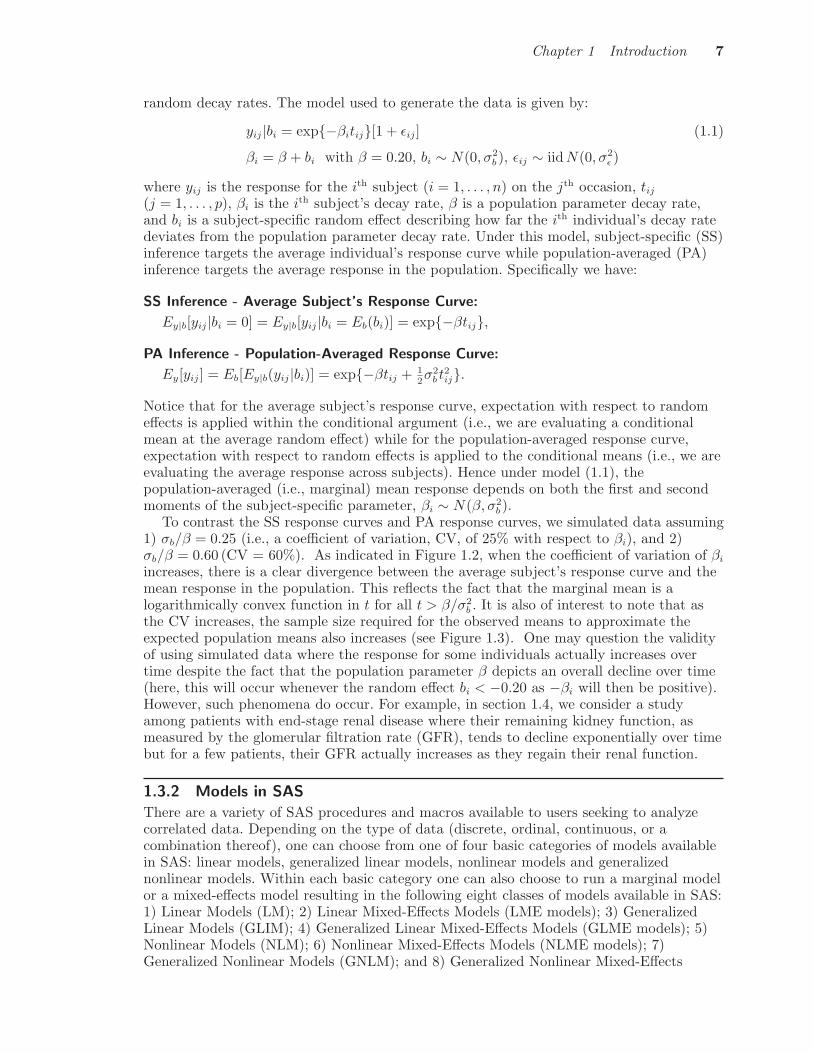
random decay rates. The model used to generate the data is given by:

yij|bi = exp{−βitij}[1 + εij]

βi = β + bi with β = 0.20, bi ∼ N(0, σ2b ), εij ∼ iidN(0, σ2

ε )

(1.1)

where yij is the response for the ith subject (i = 1, . . . , n) on the jth occasion, tij

(j = 1, . . . , p), βi is the ith subject’s decay rate, β is a population parameter decay rate,and bi is a subject-specific random effect describing how far the ith individual’s decay ratedeviates from the population parameter decay rate. Under this model, subject-specific (SS)inference targets the average individual’s response curve while population-averaged (PA)inference targets the average response in the population. Specifically we have:

SS Inference - Average Subject’s Response Curve:

Ey|b[yij|bi = 0] = Ey|b[yij|bi = Eb(bi)] = exp{−βtij},

PA Inference - Population-Averaged Response Curve:

Ey[yij] = Eb[Ey|b(yij |bi)] = exp{−βtij + 12σ2

b t2ij}.

Notice that for the average subject’s response curve, expectation with respect to randomeffects is applied within the conditional argument (i.e., we are evaluating a conditionalmean at the average random effect) while for the population-averaged response curve,expectation with respect to random effects is applied to the conditional means (i.e., we areevaluating the average response across subjects). Hence under model (1.1), thepopulation-averaged (i.e., marginal) mean response depends on both the first and secondmoments of the subject-specific parameter, βi ∼ N(β, σ2

b ).To contrast the SS response curves and PA response curves, we simulated data assuming

1) σb/β = 0.25 (i.e., a coefficient of variation, CV, of 25% with respect to βi), and 2)σb/β = 0.60 (CV = 60%). As indicated in Figure 1.2, when the coefficient of variation of βi

increases, there is a clear divergence between the average subject’s response curve and themean response in the population. This reflects the fact that the marginal mean is alogarithmically convex function in t for all t > β/σ2

b . It is also of interest to note that asthe CV increases, the sample size required for the observed means to approximate theexpected population means also increases (see Figure 1.3). One may question the validityof using simulated data where the response for some individuals actually increases overtime despite the fact that the population parameter β depicts an overall decline over time(here, this will occur whenever the random effect bi < −0.20 as −βi will then be positive).However, such phenomena do occur. For example, in section 1.4, we consider a studyamong patients with end-stage renal disease where their remaining kidney function, asmeasured by the glomerular filtration rate (GFR), tends to decline exponentially over timebut for a few patients, their GFR actually increases as they regain their renal function.

1.3.2 Models in SAS

There are a variety of SAS procedures and macros available to users seeking to analyzecorrelated data. Depending on the type of data (discrete, ordinal, continuous, or acombination thereof), one can choose from one of four basic categories of models availablein SAS: linear models, generalized linear models, nonlinear models and generalizednonlinear models. Within each basic category one can also choose to run a marginal modelor a mixed-effects model resulting in the following eight classes of models available in SAS:1) Linear Models (LM); 2) Linear Mixed-Effects Models (LME models); 3) GeneralizedLinear Models (GLIM); 4) Generalized Linear Mixed-Effects Models (GLME models); 5)Nonlinear Models (NLM); 6) Nonlinear Mixed-Effects Models (NLME models); 7)Generalized Nonlinear Models (GNLM); and 8) Generalized Nonlinear Mixed-Effects



Figure 1.3 Observed and expected marginal means for different sample sizes

Models (GNLME models). The models within any one class are determined throughspecification of the moments and possibly the distribution functions under which the dataare generated. Moment-based specifications usually entail specifying unconditional(marginal) or conditional (mixed-effects) means and variances in terms of their dependenceon covariates and/or random effects. Using the term “subject” to refer to an individual,subject, cluster or experimental unit, we adopt the following general notation which we useto describe marginal or conditional moments and/or likelihood functions.

Notation

y is a response vector for a given subject. Within a given context or unless otherwisenoted, lower case lettering y (or y) will be used to denote either the underlying randomvector (or variable) or its realization.β is a vector of fixed-effects parameters associated with first-order moments (i.e.,marginal or conditional means).b is a vector of random-effects (possibly multi-level) which, unless otherwise indicated, isassumed to have a multivariate normal distribution, b ∼ N(0,Ψ), withvariance-covariance matrix Ψ = Ψ(θb) that depends on a vector of between-subjectvariance-covariance parameters, say θb.X is a matrix of within- and between-subject covariates linking the fixed-effectsparameter vector β to the marginal or conditional mean.Z is a matrix of within-subject covariates contained in X that directly link the randomeffects to the conditional mean.μ(X, β, Z, b) = μ(β, b) = E(y|b) is the conditional mean of y given random effects b.



Table 1.1 Hierarchy of models in SAS according to mean structure and cumulative distribution function (CDF)

Marginal Models Mixed-Effects Models

Model μ(X, β) CDF Model μ(X, β, Z, b) CDF

LM Xβ Normal LME Xβ + Zb NormalGLIM g−1(Xβ) General GLME g−1(Xβ + Zb) GeneralNLM f(X, β) Normal NLME f(X, β, b) Normal

GNLM f(X, β) General GNLME f(X, β, b) General

Λ(X, β, Z, b, θw) = Λ(β, b, θw) = V ar(y|b) is the conditional covariance matrix of ygiven random effects b. This matrix may depend on an additional vector, θw, ofwithin-subject variance-covariance parameters.μ(X, β) = μ(β) = E(y) is the marginal mean of y except for mixed models where themarginal mean μ(X, β, Z, θb) = E(y) may depend on θb as well as β (e.g., see the PAmean response for model (1.1)).Σ(β, θ) = V ar(y) is the marginal variance-covariance of y that depends on between-and/or within-subject covariance parameters, θ = (θb, θw) and possibly on thefixed-effects regression parameters β.

There is an inherent hierarchy to these models as suggested in Table 1.1. Specifically,linear models can be considered a special case of generalized linear models in that thelatter allow for a broader class of distributions and a more general mean structure given byan inverse link function, g−1(Xβ), which is a monotonic invertible function linking themean, E(y), to a linear predictor, Xβ, via the relationship g(E(y)) = Xβ. LikewiseGaussian-based linear models are a special case of Gaussian-based nonlinear models in thatthe latter allow for a more general nonlinear mean structure, f(X, β), rather than one thatis strictly linear in the parameters of interest. Finally, generalized linear models are aspecial case of generalized nonlinear models in that the latter, in addition to allowing for abroader class of distributions, also allow for more general nonlinear mean structures of theform f(X, β). That is, generalized nonlinear models do not require a mean structure thatis an invertible monotonic function of a linear predictor as is the case for generalized linearmodels. In like fashion, within any row of Table 1.1, one can consider the marginal modelas a special case of the mixed-effect model in that the former can be obtained by merelysetting the random effects of the mixed-effects model to 0. We also note that sincenonlinear mixed models do not require specification of a conditional linear predictor,Xβ + Zb, the conditional mean, f(X, β, b), may be specified without reference to Z. Thisis because the fixed and random effects parameters, β and b, will be linked to theappropriate covariates through specification of the function f and its relationship to adesign matrix X that encompasses Z.

The generalized nonlinear mixed-effects (GNLME) model is the most general modelconsidered in that it combines the flexibility of a generalized linear model in terms of itsability to specify non-Gaussian distributions, and the flexibility of a nonlinear model interms of its ability to specify more general mean structures. One might wonder, then, whySAS does not develop a single procedure based on the GNLME model rather than thevarious procedures currently available in SAS. The answer is simple. The variousprocedures specific to linear (MIXED, GENMOD and GLIMMIX) and generalized linearmodels (GENMOD, GLIMMIX) offer specific options and computational features that takefull advantage of the inherent structure of the underlying model (e.g., the linearity of allparameters, both fixed and random, in the LME model, or the monotonic transformationthat links the mean function to a linear predictor in a generalized linear model). Suchflexibility is next to impossible to incorporate under NLME and GNLME models, both of



which can be fit to data using either the SAS procedure NLMIXED or the SAS macro%NLINMIX. A “road map” linking the SAS procedures and their key statements/optionsto these various models is presented in Table 1.2 of the summary section at the end of thischapter.

Finally, we shall assume throughout that the design matrices, X and Z, are of full ranksuch that, where indicated, all matrices are invertible. In those cases where we are dealingwith less than full rank design matrices and matrices of the form X ′AX, for example, arenot of full rank, the expression (X ′AX)−1 will be understood to represent a generalizedinverse of X ′AX.

1.3.3 Alternative approaches

Alternative approaches to modeling correlated response data include the use of conditionaland/or transition models as well as hierarchical Bayesian models. Texts by Diggle, Liangand Zeger (1994) and Molenberghs and Verbeke (2005), for example, provide an excellentsource of information on conditional and transition models for longitudinal data. Also, withthe advent of Markov Chain Monte Carlo (MCMC) and other techniques for generatingsamples from Bayesian posterior distributions, interested practitioners can opt for a fullBayesian approach to modeling correlated data as exemplified in the texts by Carlin andLouis (2000) and Gelman et. al. (2004). A number of Bayesian capabilities were madeavailable with the release of SAS 9.2 including the MCMC procedure. With PROC MCMC,users can fit a variety of Bayesian models using a general purpose MCMC simulationprocedure.

1.4 Some examplesIn this section, we present just a few examples illustrating the different types of responsedata, covariates, and models that will be discussed in more detail in later chapters.

Soybean Growth Data

Davidian and Giltinan (1993, 1995) describe an experimental study in which the growthpatterns of two genotypes of soybeans were to be compared. The essential features of thestudy are as follows:

• The experimental unit or cluster is a plot of land• Plots were sampled 8-10 occasions (times) within a calendar year• Six plants were randomly selected at each occasion and the average leaf weight per plant

was calculated for a plot• Response variable:

– yij = average leaf weight (g) per plant for ith plot on the jth occasion (time) within acalendar year (i = 1, . . . , n = 48 plots; 16 plots per each of the calendar years 1988, 1989and 1990; j = 1, . . . , pi with pi = 8 to 10 measurements per calendar year)

• One within-unit covariate:– tij =days after planting for ith plot on the jth occasion

• Two between-unit covariates:– Genotype of Soybean (F=commercial, P=experimental) denoted by

a1i =

{0, if commercial (F)1, if experimental (P)



Figure 1.4 Soybean growth data

– Calendar Year (1988, 1989, 1990) denoted by two indicator variables,

a2i =

{0, if year is 1988 or 19901, if year is 1989

a3i =

{0, if year is 1988 or 19891, if year is 1990

• Goal: compare the growth patterns of the two genotypes of soybean over the threegrowing seasons represented by calendar years 1988-1990.

This is an example of an experimental study involving clustered longitudinal data inwhich the response variable, y =average leaf weight per plant (g), is measured over timewithin plots (clusters) of land. In each of the three years, 1988, 1989 and 1990, 8 differentplots of land were seeded with the genotype Forrest (F) representing a commercial strain ofseeds and 8 different plots were seeded with genotype Plant Introduction #416937 (P), anexperimental strain of seeds. During the growing season of each calendar year, six plantswere randomly sampled from each plot on a weekly basis (starting roughly two weeks afterplanting) and the leaves from these plants were collected and weighed yielding an averageleaf weight per plant, y, per plot. A plot of the individual profiles, shown in Figure 1.4,suggest a nonlinear growth pattern which Davidian and Giltinan modeled using a nonlinear



mixed-effects logistic growth curve model. One plausible form of this model might be

yij = f(x′ij, β, bi) + εij

= f(x′ij, βi) + εij

=βi1

1 + exp {βi3(tij − βi2)}+ εij

βi =

⎛⎝βi1

βi2

βi3

⎞⎠ =

⎛⎝β01 + β11a1i + β21a2i + β31a3i

β02 + β12a1i + β22a2i + β32a3i

β03 + β13a1i + β23a2i + β33a3i

⎞⎠+

⎛⎝bi1

bi2

bi3

⎞⎠

(1.2)

where yij is the average leaf weight per plant for the ith plot on the jth occasion,f(x′

ij, β, bi) = f(x′ij, βi) = βi1/

[1 + exp{βi3(tij − βi2)}

]is the conditional mean response

for the ith plot on the jth occasion, x′ij =

(1 tij a1i a2i a3i

)is the vector of within- and

between-cluster covariates associated with the population parameter vector,β

′ =(β01 β11 β21 β31 β02 . . . β23 β33

)on the jth occasion. The first two columns of

x′ij, say z′

ij =(1 tij

), is the vector of within-cluster covariates associated with the

cluster-specific random effects, b′i =(bi1 bi2 bi3

)on the jth occasion, and εij is the

intra-cluster (within-plot or within-unit) error on the jth occasion. The vector ofrandom-effects are assumed to be iid N(0, Ψ) where Ψ is a 3× 3 arbitrary positive definitecovariance matrix. One should note that under this particular model, we are investigatingthe main effects of genotype and calendar year on the mean response over time.

The vector β′i =(βi1 βi2 βi3

)may be regarded as a cluster-specific parameter vector

that uniquely describes the mean response for the ith plot with βi1 > 0 representing thelimiting growth value (asymptote), βi2 > 0 representing soybean “half-life” (i.e., the timeat which the soybean reaches half its limiting growth value), and βi3 < 0 representing thegrowth rate. It may be written in terms of the linear random-effects model

βi = Aiβ + Bibi = Aiβ + bi

where

Ai =

⎛⎝1 a1i a2i a3i 0 0 0 0 0 0 0 00 0 0 0 1 a1i a2i a3i 0 0 0 00 0 0 0 0 0 0 0 1 a1i a2i a3i

⎞⎠is a between-cluster design matrix linking the between-cluster covariates, genotype andcalendar year, to the population parameters β while Bi is an incidence matrix of 0’s and1’s indicating which components of βi are random and which are strictly functions of thefixed-effect covariates. In our current example, all three components of βi are assumedrandom and hence Bi = I3 is simply the identity matrix. Suppose, however, that thehalf-life parameter, βi2, was assumed to be a function solely of the fixed-effects covariates.Then Bi would be given by

Bi =

⎛⎝1 00 00 1

⎞⎠with b

′i =(bi1 bi3

). Note, too, that we can express the between-unit design matrix more

conveniently as Ai = I3 ⊗(1 a1i a2i a3i

)where ⊗ is the direct product operator (or

Kronecker product) linking the dimension of βi via the identity matrix I3 to thebetween-unit covariate vector, a′

i =(1 a1i a2i a3i

). The ⊗ operator is a useful tool



which we will have recourse to use throughout the book and which is described more fullyin Appendix A.

Finally, by assuming the intra-cluster errors εij are iid N(0, σ2w), model (1.2) may be

classified as a nonlinear mixed-effects model (NLME) having conditional means expressedin terms of a nonlinear function, i.e., E(yij|bi) = μ(x′

ij, β, z′ij, bi) = f(x′

ij, β, bi), asrepresented using the general notation of Table 1.1. In this case, inference with respect tothe population parameters β and θ = (θb, θw) = (vech(Ψ), σ2

w) will be cluster-specific inscope in that the function f , when evaluated at bi = 0, describes what the average soybeangrowth pattern is for a “typical plot.”

Respiratory Disorder Data

Koch et. al. (1990) and Stokes et. al. (2000) analyzed data from a multicenter randomizedcontrolled trial for patients with a respiratory disorder. The trial was conducted in twocenters in which patients were randomly assigned to one of two treatment groups: an activetreatment group or a placebo control group (0 = placebo, 1 = active). The initial outcomevariable of interest was patient status which is defined in terms of the ordinal categoricalresponses: 0 = terrible, 1 = poor, 2 = fair, 3 = good, 4 = excellent. This categoricalresponse was obtained both at baseline and at each of four visits (visit 1, visit 2, visit 3,visit 4) during the course of treatment. Here we consider an analysis obtained bycollapsing the data into a discrete binary outcome with the primary focus being acomparison of the average response of patients. The essential components of the study arelisted below (the SAS variables are listed in parentheses).

• The experimental unit is a patient (identified by SAS variable ID)• The initial outcome variable was patient status defined by the ordinal response: 0 =

terrible, 1 = poor, 2 = fair, 3 = good, 4 = excellent• Response variable (y):

– The data were collapsed into a simple binary response as

yij =

{0 = negative response if (terrible, poor, or fair)1 = positive response if (good, excellent)

which is the ith patient’s response obtained on the jth visit• One within-unit covariate:– Visit (1, 2, 3, or 4) defined here by the indictor variables (Visit)

vij =

{1, if visit j

0, otherwise• Five between-unit covariates:

– Treatment group (Treatment) defined as ’P’ for placebo or ’A’ for active.

a1i =

{0, if placebo1, if active

(this indicator is labeled Drug0)

– Center (Center)

a2i =

{0, if center 11, if center 2

(this indicator is labeled Center0)

– Gender (Gender) defined as 0 = male, 1 = female

a3i =

{0, if male1, if female

(this indicator is labeled Sex)

– Age at baseline (Age)a4i =patient age



Figure 1.5 A plot of the proportion of positive responses by visit and drug for the respiratory disorder data

– Response at baseline (Baseline),

a5i =

{0 = negative,1 = positive

(this indicator is labeled y0)

• Goal: determine if there is a treatment effect after adjusting for center, gender, age andbaseline differences.

A plot of the proportion of positive responses at each visit according to treatment groupis shown in Figure 1.5. In this example, previous authors (Koch et. al., 1977; Koch et. al.,1990) fit the data using several different marginal models resulting in a population-averagedapproach to inference. One family of such models is the family of marginal generalizedlinear models (GLIM’s) with working correlation structure. For example, under theassumption of a working independence structure across visits and assuming there is no visiteffect, one might fit this data to a binary logistic regression model of the form

E(yij) = μij(x′ij, β) = g−1(x′

ijβ)

=exp{x′

ijβ}1 + exp{x′

ijβ}x′

ijβ = β0vij + β1a1i + β2a2i + β3a3i + β4a4i + β5a5i

V ar(yij) = μij(x′ij, β)[1 − μij(x′

ij, β)] = μij(1 − μij)

(1.3)

where μij = μij(x′ij, β) = Pr(yij = 1|xij) is the probability of a positive response on the jth

visit, x′ij =

(vij a1i a2i a3i a4i a5i

)is the design vector of within- and between-unit



covariates on the jth visit and β′ =(β0 β1 β2 β3 β4 β5

)is the parameter vector

associated with the mean response. Here, we do not model a visit effect but rather assumea common visit effect that is reflected in the overall intercept parameter, β0 (i.e., since wealways have vij = 1 on the jth visit, we can simply replace β0vij with β0). In matrixnotation, model (1.3) may be written as

E(yi) = μi(X i, β) = g−1(X iβ)

V ar(yi) = Σi(β) = H i(μi)1/2I4H i(μi)

1/2

where

yi =

⎛⎜⎝yi1

yi2

yi3

yi4

⎞⎟⎠ , X i =

⎛⎜⎝x′i1

x′i2

x′i3

x′i4

⎞⎟⎠ ,

and H i(μi) is the 4 × 4 diagonal variance matrix with V ar(yij) = μij(1 − μij) as the jth

diagonal element and H i(μi)1/2 is the square root of H i(μi) which, for arbitrary positivedefinite matrices, may be obtained via the Cholesky decomposition. To accommodatepossible correlation among binary responses taken on the same subject across visits, we canuse a generalized estimating equation (GEE) approach in which robust standard errors arecomputed using the so-called empirical sandwich estimator (e.g., see §4.2 of Chapter 4). Analternative GEE approach might assume an overdispersion parameter φ and “working”correlation matrix Ri(α) such that

V ar(yi) = Σi(β, θ) = φH i(μi)1/2Ri(α)H i(μi)

1/2

where θ = (α, φ). Commonly used working correlation structures include workingindependence [i.e., Ri(α) = I4 as above], compound symmetry and first-orderautoregressive. Alternatively, one can extend the GLIM in (1.3) to a generalized linearmixed-effects model (GLME) by simply adding a random intercept term, bi, to the linearpredictor, i.e.,

x′ijβ + bi = β0vij + β1a1i + β2a2i + β3a3i + β4a4i + β5a5i + bi.

This will induce a correlation structure among the repeated binary responses via therandom intercepts shared by patients across their visits.

In Chapters 4-5, we shall consider analyses based on both marginal and mixed-effectslogistic regression thereby allowing one to contrast PA versus SS inference. With respect tomarginal logistic regression, we will present results from a first-order and second-ordergeneralized estimating equation approach.

Epileptic Seizure Data

Thall and Vail (1990) and Breslow and Clayton (1993) used Poisson regression to analyzeepileptic seizure data from a randomized controlled trial designed to compare theeffectiveness of progabide versus placebo to reduce the number of partial seizures occurringover time. The key attributes of the study are summarized below (SAS variables denoted inparentheses).

• The experimental unit is a patient (ID)• The data consists of the number of partial seizures occurring over a two week period on

each of four successive visits made by patients receiving one of two treatments(progabide, placebo).



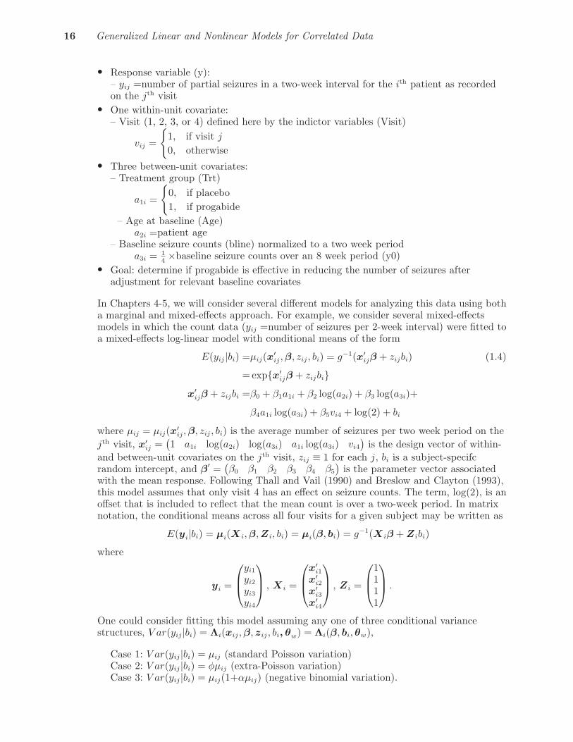
• Response variable (y):– yij =number of partial seizures in a two-week interval for the ith patient as recordedon the jth visit

• One within-unit covariate:– Visit (1, 2, 3, or 4) defined here by the indictor variables (Visit)

vij =

{1, if visit j

0, otherwise• Three between-unit covariates:

– Treatment group (Trt)

a1i =

{0, if placebo1, if progabide

– Age at baseline (Age)a2i =patient age

– Baseline seizure counts (bline) normalized to a two week perioda3i = 1

4×baseline seizure counts over an 8 week period (y0)

• Goal: determine if progabide is effective in reducing the number of seizures afteradjustment for relevant baseline covariates

In Chapters 4-5, we will consider several different models for analyzing this data using botha marginal and mixed-effects approach. For example, we consider several mixed-effectsmodels in which the count data (yij =number of seizures per 2-week interval) were fitted toa mixed-effects log-linear model with conditional means of the form

E(yij|bi) =μij(x′ij, β, zij, bi) = g−1(x′

ijβ + zijbi)

= exp{x′ijβ + zijbi}

x′ijβ + zijbi =β0 + β1a1i + β2 log(a2i) + β3 log(a3i)+

β4a1i log(a3i) + β5vi4 + log(2) + bi

(1.4)

where μij = μij(x′ij, β, zij, bi) is the average number of seizures per two week period on the

jth visit, x′ij =

(1 a1i log(a2i) log(a3i) a1i log(a3i) vi4

)is the design vector of within-

and between-unit covariates on the jth visit, zij ≡ 1 for each j, bi is a subject-specifcrandom intercept, and β

′ =(β0 β1 β2 β3 β4 β5

)is the parameter vector associated

with the mean response. Following Thall and Vail (1990) and Breslow and Clayton (1993),this model assumes that only visit 4 has an effect on seizure counts. The term, log(2), is anoffset that is included to reflect that the mean count is over a two-week period. In matrixnotation, the conditional means across all four visits for a given subject may be written as

E(yi|bi) = μi(X i, β, Zi, bi) = μi(β, bi) = g−1(X iβ + Zibi)

where

yi =

⎛⎜⎝yi1

yi2

yi3

yi4

⎞⎟⎠ , X i =

⎛⎜⎝x′i1

x′i2

x′i3

x′i4

⎞⎟⎠ , Zi =

⎛⎜⎝1111

⎞⎟⎠ .

One could consider fitting this model assuming any one of three conditional variancestructures, V ar(yij|bi) = Λi(xij, β, zij, bi, θw) = Λi(β, bi, θw),

Case 1: V ar(yij|bi) = μij (standard Poisson variation)Case 2: V ar(yij|bi) = φμij (extra-Poisson variation)Case 3: V ar(yij|bi) = μij(1+αμij) (negative binomial variation).



In the first case, Λi(β, bi, θw) = μij(β, bi) and there is no θw parameter. In the second case,we allow for conditional overdispersion in the form of Λi(β, bi, θw) = φμij(β, bi) whereθw = φ while in the third case, over-dispersion in the form of a negative binomial modelwith Λi(β, bi, θw) = μij(β, bi)(1 + αμij(β, bi)) is considered with θw = α. The conditionalnegative binomial model coincides with a conditional gamma-Poisson model which isobtained by assuming the conditional rates within each two-week interval are furtherdistributed conditionally as a gamma random variable. This allows for a specific form ofconditional overdispersion which may or may not make much sense in this setting.Assuming bi ∼iid N(0, σ2

b ), all three cases result in models that belong to the class ofGLME models. However, the models in the first and third cases are based on a well-definedconditional distribution (Poisson in case 1 and negative binomial in case 3) which allowsone to estimate the model parameters using maximum likelihood estimation. Under thissame mixed-effects setting, other covariance structures could also be considered some ofwhich when combined with the assumption of a conditional Poisson distribution yield aGNLME model generally not considered in most texts.

ADEMEX Data

Paniagua et. al. (2002) summarized results of the ADEMEX trial, a randomizedmulti-center trial of 965 Mexican patients designed to compare patient outcomes (e.g.,survival, hospitalization, quality of life, etc.) among end-stage renal disease patientsrandomized to one of two dose levels of continuous ambulatory peritoneal dialysis (CAPD).While patient survival was the primary endpoint, there were a number of secondary andexploratory endpoints investigated as well. One such endpoint was the estimation andcomparison of the decline in the glomerular filtration rate (GFR) among incident patientsrandomized to the standard versus high dose of dialysis. There were several challenges withthis objective as described below. The essential features of this example are as follows:

• The experimental unit is an incident patient• Response variables:

– yij =glomerular filtration rate (GFR) of the kidney (ml/min) for ith subject on the jth

occasion– Ti =patient survival time in months

• One within-unit covariate:– tij =months after randomization

• Six between-unit covariates:– Treatment group (standard dose, high dose)

a1i =

{0, if control = standard dose1, if intervention = high dose

– Gender

a2i =

{0, if male1, if female

– Age at baselinea3i =patient age

– Presence or absence of diabetes at baseline

a4i =

{0, if non-diabetic1, if diabetic

– Baseline value of albumina5i =serum albumin (g/dL)

- Baseline value of normalized protein nitrogen appearance (nPNA)a6i =nPNA (g/kg/day)



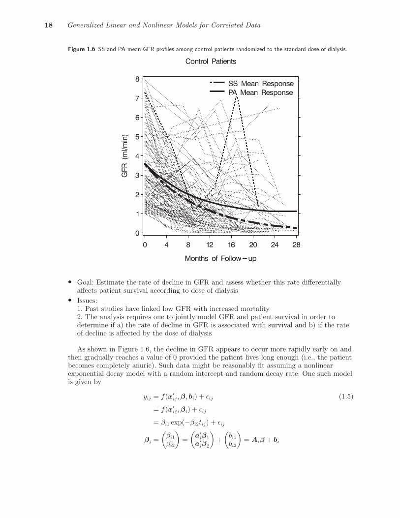
Figure 1.6 SS and PA mean GFR profiles among control patients randomized to the standard dose of dialysis.

• Goal: Estimate the rate of decline in GFR and assess whether this rate differentiallyaffects patient survival according to dose of dialysis

• Issues:1. Past studies have linked low GFR with increased mortality2. The analysis requires one to jointly model GFR and patient survival in order todetermine if a) the rate of decline in GFR is associated with survival and b) if the rateof decline is affected by the dose of dialysis

As shown in Figure 1.6, the decline in GFR appears to occur more rapidly early on andthen gradually reaches a value of 0 provided the patient lives long enough (i.e., the patientbecomes completely anuric). Such data might be reasonably fit assuming a nonlinearexponential decay model with a random intercept and random decay rate. One such modelis given by

yij = f(x′ij, β, bi) + εij

= f(x′ij, βi) + εij

= βi1 exp(−βi2tij) + εij

βi =(

βi1

βi2

)=(

a′iβ1

a′iβ2

)+(

bi1

bi2

)= Aiβ + bi

(1.5)



where a′i =(1 a1i a2i a3i a4i a5i a6i

)is the between-subject design vector,

x′ij = (tij, a

′i) is the vector of within- and between-subject covariates on the jth occasion,

a′iβ1 + bi1 = β01 + β11a1i + β21a2i + β31a3i + β41a4i + β51a5i + β61a6i + bi1

a′iβ2 + bi2 = β02 + β12a1i + β22a2i + β32a3i + β42a4i + β52a5i + β62a6i + bi2

are linear predictors for the intercept (βi1) and decay rate (βi2) parameters, respectively,b′i =(bi1 bi2

)are the random intercept and decay rate effects, and β

′ = (β′1, β

′2) is the

corresponding population parameter vector with β′1 =(β01 β11 β21 β31 β41 β51 β61

)denoting the population intercept parameters andβ

′2 =(β02 β12 β22 β32 β42 β52 β62

)the population decay rate parameters. Here

Ai = I2 ⊗ a′i is the between-subject design matrix linking the covariates ai to β while

εij ∼iid N(0, σ2w) independent of bi.

Figure 1.6 reflects a reduced version of this model in which the subject-specific interceptand decay rate parameters are modeled as a simple linear function of the treatment grouponly, i.e.,

βi1 = β01 + β11a1i + bi1

βi2 = β02 + β12a1i + bi2.

What is shown in Figure 1.6 is the estimated marginal mean profile (i.e., PA meanresponse) for the patients randomized to the control group. This PA mean response isobtained by averaging over the individual predicted response curves while the averagepatient’s mean profile (i.e., the SS mean response) is obtained by simply plotting thepredicted response curve achieved when one sets the random effects bi1 and bi2 equal to 0.As indicated previously (page 7), this example illustrates how one can have arandom-effects exponential decay model that can predict certain individuals as having anincreasing response over time. In this study, for example, two patients (one from eachgroup) had a return of renal function while others showed either a modest rise or no changein renal function. The primary challenge here is to jointly model the decline in GFR andpatient survival using a generalized nonlinear mixed-effects model that allows one toaccount for correlation in GFR values over time as well as determine if there is anyassociation between the rate of decline in GFR over time and patient survival.

1.5 Summary featuresWe summarize here a number of features associated with the analysis of correlated data.First, since the response variables exhibit some degree of dependency as measured bycorrelation among the responses, most analyses may be classified as being essentiallymultivariate in nature. With repeated measurements and clustered data, for example, theanalysis requires combining cross-sectional (between-cluster, between-subject, inter-subject)methods with time-series (within-cluster, within-subject, intra-subject) methods.

Second, the type of model one uses, marginal versus mixed, determines and/or limitsthe type of correlation structure one can model. In marginal models, correlation isaccounted for by directly specifying an intra-subject or intra-cluster covariance structure.In mixed-effects models, a type of intraclass correlation structure is introduced throughspecification of subject-specific random effects. Specifically, intraclass correlation occurs asa result of having random effect variance components that are shared across measurementswithin subjects. Along with specifying what type of model, marginal or mixed, is neededfor inferential purposes, one must also select what class of models is most appropriatebased on the type of response variable being measured (e.g., continuous, ordinal, count ornominal) and its underlying mean structure. By specifying both the class of models and



Table 1.2 A summary of the different classes of models and the type of model within a class that are available

for the analysis of correlated response data. 1. The SAS macro %NLINMIX iteratively calls the MIXED procedure

when fitting nonlinear models. 2. NLMIXED can be adpated to analyze marginal correlation structures (see §4.4,

§4.5.2, §4.5.3, §4.5.4, §5.3.3).

Types of SAS Type of Model

Class of Models Data PROC Marginal2. Mixed

Linear Continuous MIXED REPEATED RANDOM

GLIMMIX RANDOM/RSIDE RANDOM

Generalized Linear Continuous

Ordinal

Count

Binary

GENMOD

GLIMMIX

NLMIXED

REPEATED

RANDOM/RSIDE

−

−RANDOM

RANDOM

Generalized Nonlinear Continuous

Ordinal

Count

Binary

NLMIXED

%NLINMIX1.

−REPEATED

RANDOM

RANDOM

type of model within a class, an appropriate SAS procedure can then be used to analyzethe data. Summarized in Table 1.2 are the three major classes of models used to analyzecorrelated response data and the SAS procedure(s) and corresponding proceduralstatements/options for conducting such an analysis.

Another feature worth noting is that studies involving clustered data or repeatedmeasurements generally lead to efficient within-unit comparisons but inefficientbetween-unit comparisons. This is evident with split-plot designs where we have efficientsplit-plot comparisons but inefficient whole plot comparisons. In summary, some of thefeatures we have discussed in this chapter include:

• Repeated measurements, clustered data and spatial data are essentially multivariate innature due to the correlated outcome measures

• Analysis of repeated measurements and longitudinal data often requires combiningcross-sectional methods with time-series methods

• The analysis of correlated data, especially that of repeated measurements, clustereddata and spatial data can be based either on marginal or mixed-effects models.Parameters from these two types of models generally differ in that

1) Marginal models target population-averaged (PA) inference2) Mixed-effects models target subject-specific (SS) inference

• Marginal models can accommodate correlation via1) Direct specification of an intra-subject correlation structure

• Mixed-effects models can accommodate correlation via1) Direct specification of an intra-subject correlation structure2) Intraclass correlation resulting from random-effects variance

components that are shared across observations within subjects• The family of models available within SAS include linear, generalized linear, nonlinear,

and generalized nonlinear models• Repeated measurements and clustered data lead to efficient within-unit comparisons

(including interactions of within-unit and between-unit covariates) but inefficientbetween-unit comparisons.


introduction - sas

Documents