Introduction Introduction

Part 2Part 2Introduction Introduction

Part 2Part 2

Chapter 1

Case of United Airlines

Kinds of problems :

• Develop master flight schedule• Forecast demand for its routes• Determine wich planes to purchase or to

lease• Assign planes and crews to the route• Set fares

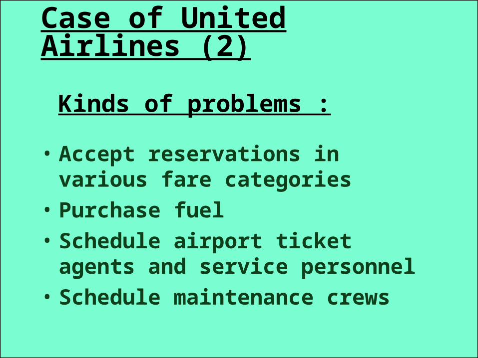
Case of United Airlines (2)

Kinds of problems :

• Accept reservations in various fare categories

• Purchase fuel• Schedule airport ticket agents and service

personnel• Schedule maintenance crews

Case of United Airlines (3)

Kinds of problems :

• Maintain service facilities• Lease airport gates• Design and monitor its frequent flyer

program

Case of United Airlines (4)

Factors impacting these decisions :

• Budget, equipment and personnel restrictions• Union agreements• FAA maintenance guidelines• Safe distance and aircraft turnaround

requirements• Flexibility to react to complications due to

weather, congestion, defects,….

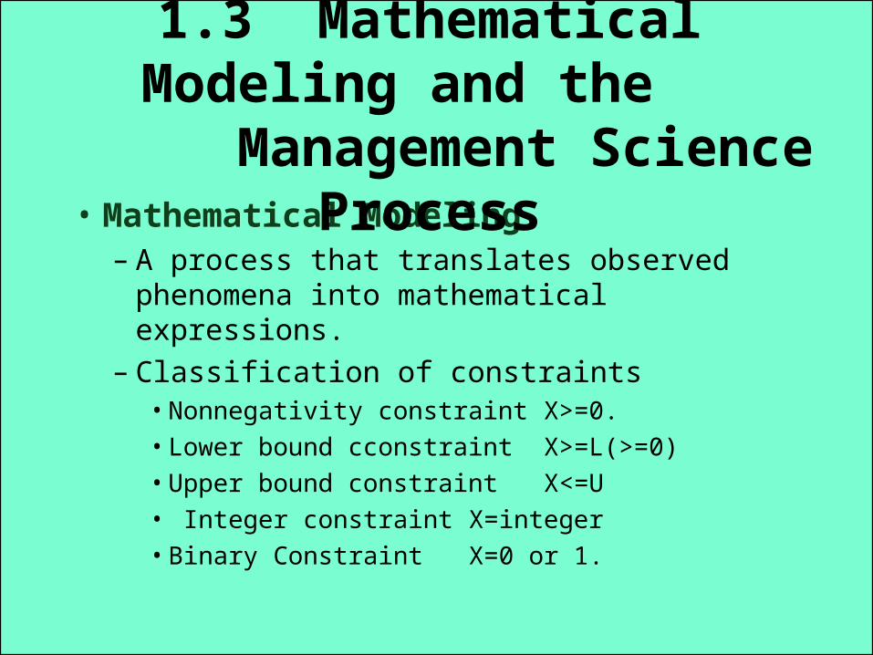
• Mathematical Modeling– A process that translates observed phenomena into

mathematical expressions.– Classification of constraints

• Nonnegativity constraint X>=0.• Lower bound cconstraint X>=L(>=0)• Upper bound constraint X<=U• Integer constraint X=integer• Binary Constraint X=0 or 1.

1.3 Mathematical Modeling and the Management Science Process

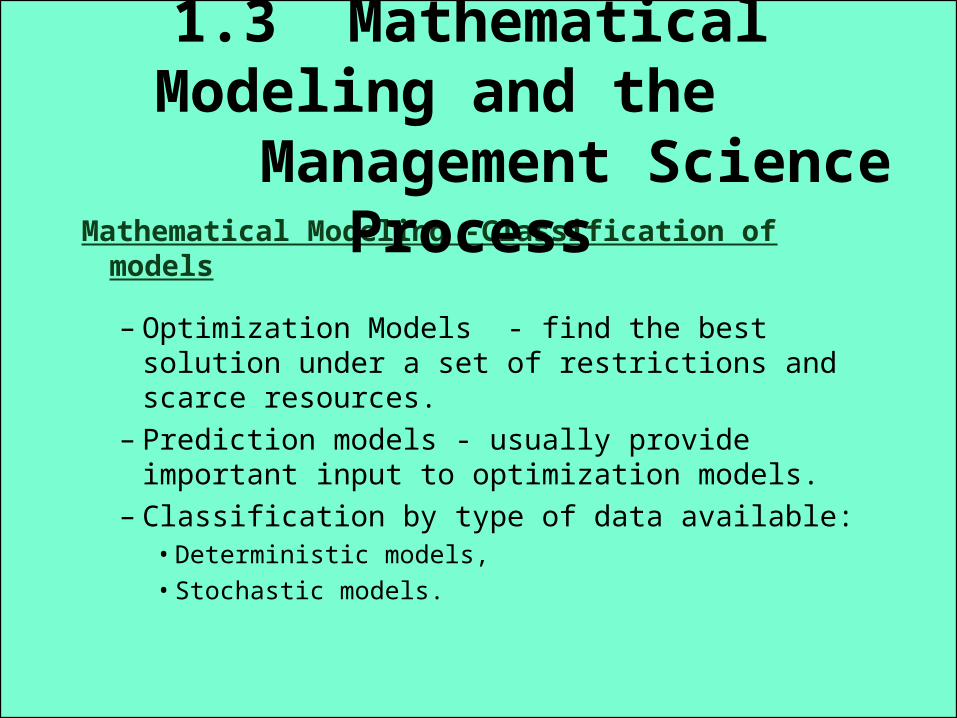
Mathematical Modeling -Classification of models

– Optimization Models - find the best solution under a set of restrictions and scarce resources.

– Prediction models - usually provide important input to optimization models.

– Classification by type of data available:• Deterministic models, • Stochastic models.

1.3 Mathematical Modeling and the Management Science Process

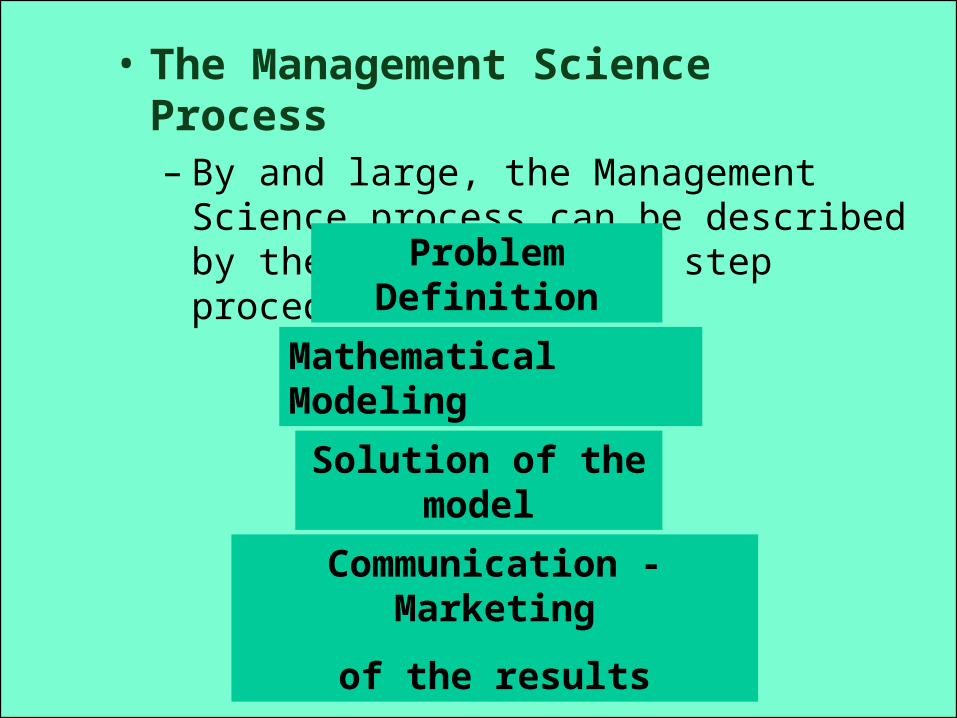
• The Management Science Process– By and large, the Management Science process can

be described by the following four step procedure.

Problem Definition

Mathematical Modeling

Solution of the model

Communication -Marketing

of the results

• The Team Concept– For large scale projects an inter--disciplinarian team work is a necessity.

• Basic Steps of the Management Science Process

– Defining the Problem.

– Building a Mathematical Model.

– Solving a Mathematical Model.

2.2 Defining the Problem

• Management Science is Applied When -– Designing and implementing new operations

– Evaluating ongoing Operations and Procedures.

– Determining and recommending corrective actions.

How do we get started ?

Can we do better ?

Help !!!

2.2 Defining the Problem

• “Problems” in Applying Management Science“Fuzzy”, incomplete, conflicting data. Conflicting goals. Differing opinions among and between workers and management. Limited budgets for analyse Narrow time frame. Political “turf war”.No exact idea of what is wanted

• How to Start and How to Proceed

– Identify the problem. – Observe the problem from various points of view. – Keep things simple. – Identify constraints. – Recognize political realities.

– Work with management, get feedback .

Delta Hardware Stores : Problem Statement

• DHS has 3 warehouses in California in San Jose, Fresno and Azusa.

• Each month DHS restocks his warehouses with its own brand of paint.

• DHS has his own paint manufacturing in Phoenix.

Delta Hardware Stores : Problem Statement

• The capacity of the manufacturing is sometimes insufficient to cover the demand.

• It’s not cost effective to expand the production capacity.

• DHS has decided to subcontract to produce paints under his label

Delta Hardware Stores : Problem Statement

The problem is :

Determine a least cost distribution scheme of paint produced at its manufacturing plant and shipments from the subcontractor to meet the demand of the warehouses.

Problem Definition

Mathematical Modeling

Solution of the model

Communication -Marketing

of the results

2.3 Building a Mathematical Model

• Identify Decision Variables–Which factors are controllable?

• Quantify the Objective and Constraints– Formulate the function to be optimized (profit, cost).– Formulate the requirements and/or restrictions.

Delta Hardware Stores : The decision variables

The questions are :

How much paint should be shipped this month from phoenix to the 3 stores?

How much extra paint should be shipped from the subcontractor to the 3 stores?

Delta Hardware Stores : The decision variables•

• X1 : amount shipped from Phoenix to San Jose• X2 : amount shipped from Phoenix to Fresno

• X3 : amount shipped from Phoenix to Azusa

• X4 : amount shipped from subcontractor to San Jose

• X5 : amount shipped from subcontractor to Fresno

• X6 : amount shipped from subcontractor to Azusa

2.3 Building a Mathematical Model

• Construct a Model Shell– Help focus on the exact data required.

• Gather Data – Consider time / cost issues for

• collecting, organizing and sorting relevant data• generating a solution approach• using the model

Delta Hardware Stores : The model shell

• The production capacity in Phoenix is finite.• The requirements of the 3 stores are different.• The delivery trucks carry 1000 gallons at a time.• The cost of shipping is function of the distance.• The cost of the subcontractor is higher than the

cost in DHS plant.

Delta Hardware Stores : The model shell

• To obtain the best prices, orders must be in 1000-gallon increments.

• The subcontractor charges :– a fixed fee for each 1000 gallons ordered,– a delivery charge to each of the 3 warehouses.

Delta Hardware Stores : The model shell

The objective is to minimize the total monthly costs of manufacturing, transporting and subcontracting subject to :

– the Phoenix plant cannot produce more than his capacity

– the amount ordered from the subcontractant cannot exceed a maximum limit

– the orders of the warehouses are to be fulfilled

If :• M is the manufacturing cost for 1000 gallons in Phoenix• T1, T2 ant T3 are the truckloads shipping cost from Phoenix to the 3

stores• C is the fixed purchase cost per 1000 gallons from the subcontractor• S1, S2 and S3 are the shipping charges per 1000 gallons from the

subcontractor to the 3 storesThen we have :

Min (M+T1)X1 + (M+T2)X2 + (M+T3)X3 +

(C+S1)X4 + (C+S2)X5 + (C+S3)X6

Delta Hardware Stores : The model shell

The constraints are :• number of truckloads from Phoenix cannot exceed the capacity :

X1 + X2 + X3 Q1• number of 1000-gallons ordered from the subcontractor cannot exceed

a limit :

X4 + X5 + X6 Q2• number of 1000-gallons received in the stores equals their orders :

X1 + X4 = R1

X2 + X5 = R2

X3 + X6 = R6• all shipments must be nonnegative and integer

Delta Hardware Stores : The model shell

After quantification of the parameters, we have :

Minimize 4050 X1 + 3750 X2 + 3650 X3 + 6200X4 + 6400X5 + 6100 X6

Subject to :

X1 + X2 + X3 8

X4 + X5 + X6 5

X1 + X4 = 4

X2 + X5 = 2

X3 + X6 = 5

Xi 0 and integer

Delta Hardware Stores : The model shell

Problem Definition

Mathematical Modeling

Solution of the model

Communication -Marketing

of the results

2.4 Solving a Mathematical Model• Choose an Appropriate Solution Technique

– An optimization algorithm.– A heuristic algorithm.

• Woolsey’s Laws– Managers would rather live with a problem they can’t

solve than use a technique they don’t trust…..– Managers don’t want the best solutions; they simply

want a better one…..– If the solution technique costs more than you will

save, don’t use it…..

2.4 Solving a Mathematical Model

• Generate Model Solutions• Test / Validate Model Results

– Is the solution reasonable? – Are radical changes needed? – Does it fit present and future plans?– Unacceptable results? Return to modeling.

• Perform “What--If” Analyses

Delta Hardware Stores : Model Solution

123

45678

910111213141516

A B C D E FDELTA HARDWARE

COSTS PER 1000 GALLONS AVAILABLE

(1000'S GALLONS)SAN JOSE FRESNO AZUSA

PHOENIX PLANT 4050 3750 3650 8SUBCONTRACTOR 6200 6400 6100 5

DEMAND

(1000'S GALLONS)4 2 5

SHIPMENTS TOTAL TOTAL

SAN JOSE FRESNO AZUSA SHIPPED COSTPHOENIX PLANT 1 2 5 8 48400SUBCONTRACTOR 3 0 0 3

TOTAL 4 2 5

Microsoft Excel 5.0c Answer ReportWorksheet: [DELTA.XLS]Sheet1Report Created: 12/22/96 14:37Target Cell (Min)

Cell Name Original Value Final Value$F$14 PHOENIX PLANT COST 0 48400

Adjustable Cells

Cell Name Original Value Final Value$B$14 PHOENIX PLANT SAN JOSE 0 1$C$14 PHOENIX PLANT FRESNO 0 2$D$14 PHOENIX PLANT AZUSA 0 5$B$15 SUBCONTRACTOR SAN JOSE 0 3$C$15 SUBCONTRACTOR FRESNO 0 0$D$15 SUBCONTRACTOR AZUSA 0 0

Constraints

Cell Name Cell Value Formula Status Slack$E$14 PHOENIX PLANT SHIPPED 8 $E$14<=$F$6 Binding 0$E$15 SUBCONTRACTOR SHIPPED 3 $E$15<=$F$7 Not Binding 2$B$16 TOTAL SAN JOSE 4 $B$16=$B$9 Binding 0$C$16 TOTAL FRESNO 2 $C$16=$C$9 Binding 0$D$16 TOTAL AZUSA 5 $D$16=$D$9 Binding 0$B$14 PHOENIX PLANT SAN JOSE 1 $B$14>=0 Not Binding 1$C$14 PHOENIX PLANT FRESNO 2 $C$14>=0 Not Binding 2$D$14 PHOENIX PLANT AZUSA 5 $D$14>=0 Not Binding 5$B$15 SUBCONTRACTOR SAN JOSE 3 $B$15>=0 Not Binding 3$C$15 SUBCONTRACTOR FRESNO 0 $C$15>=0 Binding 0$D$15 SUBCONTRACTOR AZUSA 0 $D$15>=0 Binding 0

Delta Hardware Stores : Model SolutionMicrosoft Excel 5.0c Sensitivity ReportWorksheet: [DELTA.XLS]Sheet1

Changing CellsFinal Reduced Objective Allowable Allowable

Cell Name Value Cost Coefficient Increase Decrease$B$14 PHOENIX PLANT SAN JOSE 1 0 4050 2150 300$C$14 PHOENIX PLANT FRESNO 2 0 3750 500 1E+30$D$14 PHOENIX PLANT AZUSA 5 0 3650 300 1E+30$B$15 SUBCONTRACTOR SAN JOSE 3 0 6200 300 2150$C$15 SUBCONTRACTOR FRESNO 0 500 6400 1E+30 500$D$15 SUBCONTRACTOR AZUSA 0 300 6100 1E+30 300

ConstraintsFinal Shadow Constraint Allowable Allowable

Cell Name Value Price R.H. Side Increase Decrease$E$14 PHOENIX PLANT SHIPPED 8 -2150 8 3 1$E$15 SUBCONTRACTOR SHIPPED 3 0 5 1E+30 2$B$16 TOTAL SAN JOSE 4 6200 4 2 3$C$16 TOTAL FRESNO 2 5900 2 1 2$D$16 TOTAL AZUSA 5 5800 5 1 3

Problem Definition

Mathematical Modeling

Solution of the model

Communication -Marketing of the results

2.5 Communicating the results

• Prepare a business report or presentation.– Be concise– Use common everyday language– Make liberal use of graphics

• Monitor the progress of the implementation

2.5 Communicating the results

• Introduction - Problem statement• Assumptions/approximations made• Solution approach - computer program used• Results - presentation/analysis• What-if analyses• Overall recommandation• Appendices

Parts of a Business Presentation

• The Management Science Process

Problem Definition

Mathematical Modeling

Solution of the model

Communication -Marketing

of the results

Advantages of using the management science approach

• Helps the DM to focus on the true goals of the problem

• Helps deal with a problem in its entirety• Helps sort out data that are relevant to the

problem• Describes the problemin concise

mathematical relationships

Advantages of using the management science approach

• Helps reveal cause-and-effect relations in the problem

• Can be used to solve complex problems with large amounts data

• Yields an optimal (or at least a good) solution

Disadvantages of using the management science approach

• Uses idealized models that may be oversimplified

• May not be cost effective

• Can be misused by untrained personel

• Requires quantification of all model input

Disadvantages of using the management science approach

• May create models requiring excessive computer ressources

• May create models that are to difficult to explain to users

• Can yield suspect or insatisfactory results due to a rapidly changing environment